Evaluation of Heterogeneous Firm Models Article (Short...
87
Tari/s, Trade and Productivity: A Quantitative Evaluation of Heterogeneous Firm Models (Short title: Tari/s, Trade and Productivity) Holger Breinlich Alejandro Cuæat September 30, 2014 Abstract We examine the quantitative predictions of heterogeneous rm in the context of the Canada - US Free Trade Agreement (CUSFTA) of 1989. We compute pre- dicted increases in trade ows and measured productivity and compare them to the post-CUSFTA increases observed in the data. Most models predict increases in measured productivity that are too low by an order of magnitude relative to predicted increases in trade ows. A multi-product rm extension that allows for within-rm productivity increases has the potential to reconcile model predictions with the data. Since the seminal contribution by Melitz (2003), heterogeneous rm models have be- come a widely used instrument in the toolkitof international economists. These models This work builds upon our earlier (unpublished) paper Trade Liberalization and Heterogeneous Firm Models: An Evaluation Using the Canada - US Free Trade Agreement. We are grateful to Andy Bernard, Gordon Hanson, Mikls Koren, Sam Kortum, Marc Melitz, Alex Michaelides and Ralph Ossa for helpful discussions. We would also like to thank seminar participants at Banco de Espaæa, CEU, Chicago, CORE, the EEA MÆlaga Meeting, EUI, Fundacin Rafael del Pino, Ko University, LSE, Munich, NBER Summer Institute, GIST and Vienna for comments and suggestions. All errors remain ours. Cuæat gratefully acknowledges nancial support by the Austrian Science Fund (FWF #AP23424- G11). Corresponding author: Holger Breinlich, University of Essex, Department of Economics, Wivenhoe Park, Colchester CO4 3SQ, United Kingdom; Email address: [email protected]. This article has been accepted for publication and undergone full peer review but has not been through the copyediting, typesetting, pagination and proofreading process, which may lead to differences between this version and the Version of Record. Please cite this article as doi: 10.1111/ecoj.12218 This article is protected by copyright. All rights reserved. Accepted Article
Transcript of Evaluation of Heterogeneous Firm Models Article (Short...

Tariffs, Trade and Productivity: A Quantitative
Evaluation of Heterogeneous Firm Models∗
(Short title: Tariffs, Trade and Productivity)
Holger Breinlich Alejandro Cuñat
September 30, 2014
Abstract
We examine the quantitative predictions of heterogeneous firm in the context
of the Canada - US Free Trade Agreement (CUSFTA) of 1989. We compute pre-
dicted increases in trade flows and measured productivity and compare them to
the post-CUSFTA increases observed in the data. Most models predict increases
in measured productivity that are too low by an order of magnitude relative to
predicted increases in trade flows. A multi-product firm extension that allows for
within-firm productivity increases has the potential to reconcile model predictions
with the data.
Since the seminal contribution by Melitz (2003), heterogeneous firm models have be-
come a widely used instrument in the ‘toolkit’of international economists. These models
∗This work builds upon our earlier (unpublished) paper “Trade Liberalization and HeterogeneousFirm Models: An Evaluation Using the Canada - US Free Trade Agreement”. We are grateful to AndyBernard, Gordon Hanson, Miklós Koren, Sam Kortum, Marc Melitz, Alex Michaelides and Ralph Ossafor helpful discussions. We would also like to thank seminar participants at Banco de España, CEU,Chicago, CORE, the EEA Málaga Meeting, EUI, Fundación Rafael del Pino, Koç University, LSE,Munich, NBER Summer Institute, GIST and Vienna for comments and suggestions. All errors remainours. Cuñat gratefully acknowledges financial support by the Austrian Science Fund (FWF #AP23424-G11). Corresponding author: Holger Breinlich, University of Essex, Department of Economics, WivenhoePark, Colchester CO4 3SQ, United Kingdom; Email address: [email protected].
This article has been accepted for publication and undergone full peer review but has not been
through the copyediting, typesetting, pagination and proofreading process, which may lead to
differences between this version and the Version of Record. Please cite this article as doi:
10.1111/ecoj.12218
This article is protected by copyright. All rights reserved.
Acc
epte
d A
rtic
le

were motivated by a number of stylized facts: (i) the existence of large productivity dif-
ferences among firms within the same industry; (ii) the higher productivity of exporting
firms as compared to non-exporting firms; (iii) the large levels of resource reallocations
across firms within industries following trade liberalization reforms; and (iv) the result-
ing gains in aggregate industry productivity. In a generalization of the Krugman (1979,
1980) model, the introduction of within-industry productivity heterogeneity and beach-
head costs enables this class of models to produce equilibria and comparative statics along
the lines of these facts.
While these models are thus qualitatively consistent with available empirical evidence,
a thorough evaluation of their quantitative predictions with regards to trade liberalization
is still at an early stage. This is despite the fact that the models’quantitative predictions
for the link between trade liberalization and changes in aggregate productivity or trade
flows are of first-order importance for economic policy and welfare analysis. In this paper,
we attempt to provide such an evaluation. We go beyond the stylized facts listed above
and ask to what extent a range of heterogeneous firm models in the tradition of Melitz
(2003) are able to quantitatively replicate the changes in trade flows and productivity
associated with a specific trade liberalization episode.
We do so in the context of the Canada - US Free Trade Agreement of 1989 (CUSFTA).
As we explain in more detail in Section 2 below, CUSFTA is an ideal setting for the
quantitative evaluation of trade liberalization episodes.1 First, it was a ‘pure’ trade
liberalization in the sense that it was not accompanied by any other important economic
reform, nor was it a response to a macroeconomic shock. Second, it was also largely
unanticipated since its ratification by the Canadian parliament was considered to be
uncertain as late as November 1988.2 Third, the main instrument of liberalization were
tariff cuts which are easily quantifiable and have a direct theoretical counterpart in all
the models we analyse. Finally, there is a substantial amount of reduced-form evidence
that CUSFTA has had a significant causal impact on both trade flows and productivity
1Also see Trefler (2004).2See Breinlich (2008) for a discussion of this point. Frizzell et al. (1989) provide a detailed account
of the political context in which the agreement was signed.
This article is protected by copyright. All rights reserved.
Acc
epte
d A
rtic
le

in the Canadian manufacturing sector (e.g. Head and Ries, 1999, 2001; Trefler, 2004).
The goal of our analysis is to evaluate to which extent different versions and exten-
sions of Melitz’s heterogeneous firm model can replicate the magnitude of trade flow and
productivity increases we observe in Canada in the post-CUSFTA period (1988-1996).
The baseline model we use for our analysis is a version of Chaney (2008), who extends
Melitz (2003) to multiple asymmetric countries and industries as well as asymmetric
trade barriers between countries. We write the model’s equilibrium conditions in changes
following Dekle et al. (2008). This allows us to express predicted increases in trade flows
and measured productivity as functions of initial trade shares, the actual observed tariff
cuts as well as a small number of additional parameters. We compute these predictions
for around 200 Canadian manufacturing sectors and compare means, variances and co-
variances of these increases across sectors to the trade flow and productivity increases
observed in the data. Throughout, we pay close attention to construct model predictions
which are directly comparable to the data. We do so by mimicking the procedures used
by Statistics Canada in computing measured trade and productivity growth as closely as
possible in the construction of our theoretical moments.3
Our central result is that our benchmark model is inherently incapable of matching
both trade and productivity increases. This is true when we use sectorial parameter
estimates obtained from other data sources, or when we choose parameters to minimize
deviations between theoretical and empirical moments via a simple GMM procedure. The
predicted increase in trade flows for a given change in tariffs is always much too large
relative to the predicted increase in measured productivity. Put differently, if we choose
parameters to match trade flows, the model substantially underpredicts the growth in
measured productivity we observe in the data.
We explore the robustness of our results in a number of ways, such as using different
approaches to computing measured productivity growth or modelling tariff cuts in the
model. We also investigate whether the baseline model’s poor performance is due to the
fact that it abstracts from many important real-world determinants of trade and produc-
3Section 3 and Appendix A discuss in detail how measured real productivity growth arises in ourmodeling frameworks despite the presence of fixed markups.
This article is protected by copyright. All rights reserved.
Acc
epte
d A
rtic
le

tivity growth (e.g., technological progress unrelated to trade liberalization, or changes in
non-tariff barriers and physical transport costs). We first show that allowing for contem-
poraneous changes in other trade barriers cannot resolve the fundamental mismatch of
trade and productivity growth. Secondly, we remove a number of sources of variation
from the data which are absent from our model. For example, we first-difference the data
to remove time-invariant trends in productivity and trade flow increases. We also project
the data on sectorial-level tariff cuts as in Trefler (2004) and use the predicted values for
a comparison to our model’s predictions. That is, we only use the variation in the data
associated with tariff cuts, which is directly comparable to the key mechanism in our
model (where tariff reductions are the only exogenous driver of trade and productivity
growth).4 These procedures lead to a better fit of the model to the data, but the overall
discrepancies remain large.
Having established the inability of our baseline model to simultaneously match trade
and productivity increases, we ask which variations in modelling features bring the
model’s predictions closer to the data. We experiment with versions of our baseline model
allowing for free entry, tradable intermediate inputs, general equilibrium effects operating
through wages, and endogenous firm-level productivity through adjustments in product
scope as in Bernard et al. (2011). We find that free entry and general equilibrium effects
do not markedly improve the model’s performance. Introducing tradable intermediates
helps somewhat, but formal over-identification tests in our GMM framework still reject
this model variant. The only model that is capable of providing a good fit to the data
and of passing our over-identification tests is the multi-product firm extension. We in-
terpret these results as evidence for the need to explicitly model within-firm productivity
increases when constructing quantitative trade models capable of explaining first-order
features of trade liberalization episodes. This is in line with a number of recent studies
highlighting within-firm productivity effects in response to freer trade, in the context of
CUSFTA but also of other trade liberalization episodes (e.g., Bustos, 2011; Lileeva and
4We always perform the same transformation on the actual and the model-generated data to preservecomparability. We explain this approach in more detail in Section 4.
This article is protected by copyright. All rights reserved.
Acc
epte
d A
rtic
le

Trefler, 2011).5
Our research contributes to several related strands in the literature. The first are
papers concerned with the design and testing of a new generation of computable gen-
eral equilibrium (CGE) models (e.g., Balistreri et al., 2011; Corcos et al. 2012). This
new generation of CGE models tries to improve the predictive performance of earlier
CGE models by explicitly modelling firm-level heterogeneity.6 Our paper highlights a
fundamental problem many of these models face when trying to predict the effects of a
reduction of trade barriers —the inability to match both trade and productivity increases,
the two variables which have been the focus of most existing theoretical and empirical
analyses of trade liberalization episodes. We also contribute to this literature by per-
forming a comparative evaluation of a wide range of popular trade models, rather than
focusing on the performance of one particular version. Finally, we look at both within-
and out-of-sample predictions and employ formal statistical tests to evaluate model per-
formance, rather than only comparing the model predictions and data in a relatively ad
hoc fashion.
Secondly, we contribute to the rapidly growing literature on quantitative trade mod-
els (e.g., Eaton and Kortum, 2002; Alvarez and Lucas, 2007; Hsieh and Ossa, 2011;
Levchenko and Zhang, 2011; Arkolakis et al., 2012; Ossa, 2012; and Costinot and
Rodríguez-Clare, 2013, for a recent overview). One of the key purposes of these pa-
pers is to compute the gains from trade in different gravity-type models and to relate the
magnitude of the predicted gains to specific model features. Obviously, the usefulness
of these exercises depends crucially on the empirical validity of the underlying modelling
frameworks in terms of their quantitative (rather than just qualitative) predictions. We
point out that a class of widely used quantitative trade models has diffi culties matching
basic adjustment patterns to freer trade, and show which model modifications provide a
5Given that the number of free parameters in the above models varies, we also look at the out-of-sample predictions of our models. That is, we estimate parameters on the pre-liberalization period(1980-1988) and compare the models’ predictions for the post-liberalization (1988-1996) period, thuscontrolling for potential problems of overfitting. Still, we find that the multiproduct extension of ourbaseline model performs best.
6See Kehoe (2005) for an evaluation of the (poor) quantitative performance of some of these earliermodels.
This article is protected by copyright. All rights reserved.
Acc
epte
d A
rtic
le

better fit to the data.
There is a also a much smaller number of papers which have recently evaluated other
aspects of the quantitative performance of models in the tradition of Melitz (2003). For
example, Lawless (2009) and Eaton et al. (2011) note the inability of these models to
explain several features of firm-level data such as the fact that firms do not enter mar-
kets according to an exact hierarchy or that exporters sell more at home than predicted.
Armenter and Koren (2014) show that Melitz-type models cannot match both the size
and the share of exporters given the observed distribution of total sales. Chaney (2013)
points out that they are unable to simultaneously match a number of stylized facts re-
garding the distribution of the geographic location and the number of foreign markets
accessed by different firms. These papers all make important contributions to improving
various quantitative predictions of Melitz-type models in the cross-section; but they do
not provide evidence for the quantitative performance of these models in predicting the
effects of trade liberalization. As we have argued above, we see this aspect as central
for economic policy and welfare analysis, and the success of Melitz-type models in ex-
plaining post-liberalization changes in productivity and trade qualitatively has certainly
contributed to their popularity. Put differently, even if Melitz-type models fail to match
important cross-sectional facts, they might still provide reasonably precise predictions
for the consequences of trade liberalization. Likewise, even if a model matches all rel-
evant cross-sectional facts, it does not automatically follow that its trade liberalization
predictions will be adequate. A good quantitative cross-sectional performance is neither
necessary nor suffi cient for quantitatively accurate time-series predictions with respect to
trade liberalization and a separate investigation is thus required.7 Finally, we again also
add to this last group of related papers by introducing formal over-identification tests
and an analysis of both within- and out-of-sample predictions.
The rest of the paper is structured as follows. In Section 2, we provide background
information on CUSFTA and take a first look at the increases in trade flows and measured7Milton Friedman famously argued that ‘... theory is to be judged by its predictive power for the
class of phenomena which it is intended to explain’. (Friedman, 1953, p.8). In our view, the central aimof Melitz-type models is to make sense of, and predictions for, the reaction of an economy to reductionsin trade barriers. Other (cross-sectional) predictions are also relevant but more secondary.
This article is protected by copyright. All rights reserved.
Acc
epte
d A
rtic
le

productivity we observe in the data. Section 3 discusses our baseline model and how
we compute our theoretical predictions. Section 4 evaluates this model’s quantitative
predictions and shows why the model is inherently incapable of matching our empirical
moments. In Section 5 we discuss different extensions of our baseline model and show
that allowing for endogenous firm-level productivity is one way of reconciling models of
the class of Melitz (2003) with the evidence. Section 6 concludes.
1 Empirical Setting
Negotiations for CUSFTA started in May 1986, were finalized in October 1987 and the
treaty was signed in early 1988. The agreement came into effect on 1 January 1989, which
was also the date of the first round of tariff cuts. Tariffs were then phased out over a
period of up to ten years with some industries opting for a swifter phase-out.
Figure 1 shows that these tariff reductions were accompanied by strong increases
in Canadian trade flows (imports plus exports to/from the U.S.) and measured labour
productivity.8 The average Canadian trade flow increase over the period 1988 to 1996 was
118%, while the increase in labour productivity was 30%. This compares to growth rates
of only 44% (trade) and 17% (labour productivity) for the pre-liberalisation period, 1980-
1988. Figure 1 also displays a high degree of heterogeneity in trade flow and productivity
changes across the 203 sectors in our data in the post-liberalization period. For example,
industries at the 5th percentile of the distribution of productivity changes observed a
decrease of close to -12% over the 1988-1996 period, or -1.5% per year. In contrast,
industries at the 95th percentile saw productivity increase by over 80% in total or 7.7% per
year. Likewise, trade flow changes range from -14% (-1.9% p.a.) at the 5th percentile to
over +400% (22% p.a.) at the 95th percentile. Using differences-in-differences estimation
and instrumental variables techniques, Trefler (2004) demonstrates a causal link between
these changes and the extent of tariff cuts across sectors.
8We use data for 203 Canadian manufacturing sectors from Trefler (2004), who uses Statistics Canadaas his original data source. We compute growth rates from data expressed in 1992 Canadian dollars using4-digit industry price and value added deflators and the 1992 US-Canadian Dollar exchange rate. Laborproductivity is calculated as value added in production activities divided by total hours worked byproduction workers. See section 4 for additional details on data construction.
This article is protected by copyright. All rights reserved.
Acc
epte
d A
rtic
le

In the light of this evidence, we focus on model predictions regarding average changes
in trade and productivity and their dispersion across sectors. This is in line with the view
that models of trade liberalisation should at least correctly predict average increases in
trade and productivity, as well as being able to account for the strong sectorial hetero-
geneity evident in the data.9 Table 1 summarizes our empirical moments. Besides the
mean and the variance of trade flow and productivity increases, we also look at the co-
variance between these increases across sectors. That is, we will be comparing the first
and second moments of these variables to their theoretical counterparts in our models.
Before moving on to a description of our baseline model, we discuss some possible
objections to our approach of comparing model predictions to empirical moments based
on trade and productivity growth. Most importantly, the only (exogenous) driver of trade
and productivity growth in our models are tariff cuts. In contrast, other determinants are
likely to be present in the data, which might make a direct comparison between theoretical
and empirical moments uninformative. We have several replies to this objection.
First, several aspects of CUSFTA suggest that it is a reasonable abstraction to rely
on models with relatively simple, tariff-reduction driven, data generating processes. In
particular, tariff cuts were by far the most important tool of liberalization under CUS-
FTA. In contrast, non-tariff barriers remained unchanged after 1988 in the sense that
the corresponding provisions in CUSFTA only amounted to a reconfirmation of earlier
multilateral obligations under the General Agreement on Tariffs and Trade (GATT).10
CUSFTA also had a ‘natural experiment’character in the sense that it was not accompa-
nied by any other important economic reform, nor was it a response to a macroeconomic
shock (see Trefler, 2004). This implies that the presence of other, unmodelled, deter-
minants of trade and productivity growth should be less important than during other
9Note that this is a less demanding test than asking the model to exactly match trade and productivitygrowth in all sectors. As we will see, however, the key problem of most of our models is to get the relativeresponse of trade and productivity growth right. This is what prevents these models from matching thedata, be it sector-by-sector or on average. A further advantage of relying on moments computed acrosssectors is that we can implement formal statistical tests within a GMM framework, once we impose thenecessary cross-sectoral parameter restrictions (see Section 3 below).10See, in particular, Chapters 5, 6 and 13 of CUSFTA (1988) on National Treatment, Technical
Standards and Government Procurement. All of these measures also have in common that they are notsector-specific and as such are unlikely to be correlated with tariff cuts. (We discuss the issue of omittedvariables correlated with tariff reductions below and in Section 4.)
This article is protected by copyright. All rights reserved.
Acc
epte
d A
rtic
le

liberalization episodes, and the resulting deviations between model predictions and data
less substantial.
We think that these points make ‘tariff-reductions only’ models a useful starting
point for our evaluation. But the presence of other, unmodelled determinants of trade
and productivity growth in the data is of course still likely. This is why in Section 4
we experiment at length with different procedures of removing variation from the data
which is likely to be driven by factors absent from our models. Most importantly, we show
that our results go through when we only rely on variation in the data associated with
reductions in tariffs. Here again, the ‘natural experiment’character of CUSFTA is useful
because it makes the variation in tariff cuts largely exogenous. Indeed, Trefler (2004)
experiments with different instrumental variable strategies and, using the same tariff
data as in this paper, finds no evidence for endogeneity problems in the corresponding
Hausman tests.
One remaining concern with relying on tariff cuts as the key driver of trade and
productivity growth in our models is that US-Canadian manufacturing tariffs were already
relatively low in 1988. Trefler (2004) discusses this issue at length, and shows that two
factors make it nevertheless plausible that CUSFTA generated the strong observed trade
and productivity responses which he finds and which we have discussed above. While
average Canadian manufacturing tariffs against the United States were only around 8%
in 1988, this average hid a substantial amount of sectorial heterogeneity. In fact, more
than a quarter of Canadian industries were protected by tariffs in excess of 10%. These
industries also tended to be characterised by low profit margins, implying that the 1988
tariffwall was high and that its removal could be expected to lead to important selection
and trade effects within Canada. Similar arguments apply to the import tariffs faced by
Canadian firms exporting to the United States which also showed a strong variation across
sectors (although the average initial tariff was somewhat lower here, at approximately
4%).
Finally, we note that even if a large part of the trade and productivity gains after
1988 was driven by factors correlated with, but distinct from, tariff reductions, this is
This article is protected by copyright. All rights reserved.
Acc
epte
d A
rtic
le

unlikely to rescue our baseline and most of our augmented models. For example, we
show in Section 4 that allowing for changes in trade barriers other than tariffs faces the
same problems of simultaneously matching trade and productivity increases. If we vary
such trade barriers to exactly match trade growth, we still substantially underestimate
productivity growth, and vice versa.
2 Description of Baseline Model
In this section, we outline our baseline model, which is a version of Chaney (2008). We de-
scribe the model setup and how we derive our equilibrium conditions in changes. We then
discuss how to construct theoretical predictions from the model which are comparable to
the empirical moments we observe in the data (see Table 1).11
Model Setup and Equilibrium Conditions
There are many countries, denoted by h and j.12 Each country admits a representative
agent, with quasi-linear preferences
Uj =∑i∈I
mij lnQij + Aj, (1)
where mij > 0 and i denotes industries. Aj denotes consumption of a homogeneous final
good. Qij denotes a Dixit-Stiglitz aggregate (manufacturing) final good i:
Qij =
[∫γ∈Γij
qij(γ)ρidγ
] 1ρi
, (2)
where ρi ∈ (0, 1) and σi ≡ 1/ (1− ρi) denotes the elasticity of substitution between any
two varieties. Choosing good A as the numéraire, utility maximisation on the upper
level yields demand functions Aj = Yj −∑
imij and Eij ≡ PijQij = mij, where Yj is
11Given that this model is a straightforward extension of Chaney (2008), we keep the descriptionof the model set up to a minimum and devote more space to the construction of the theoretical mo-ment. Further details about the model are contained in the Online Appendix to this paper (available athttp://privatewww.essex.ac.uk/~hbrein/TheAppendix_20130717.pdf).12When considering bilateral variables, we adopt the convention that h and j refer to exporting and
importing countries, respectively.
This article is protected by copyright. All rights reserved.
Acc
epte
d A
rtic
le

total expenditure per consumer. In the manufacturing goods sector, utility maximisation
yields demand function qihj(γ) = pihj (γ)−σi P σi−1ij mij.
The homogeneous good is made with labour l and a linear technology A = lA iden-
tical across countries. Manufacturing varieties are made with the production function
qi (γ) = γli (γ), where γ denotes (firm-specific) productivity. γ is iid across firms within
an industry. For tractability purposes, we assume γ to be distributed Pareto with shape
parameter aiγ and location parameter kijγ . We assume the same shape parameter for an
industry across countries, but allow it to vary across industries. The location parameter is
allowed to vary across industries and countries. Producers of the homogeneous good and
the final goods Qi operate in a perfectly competitive environment. Producers of varieties
in the manufacturing industry have instead monopoly power over their own varieties.
The homogeneous good is traded freely; supplying it to any market involves no costs.
We consider equilibria in which all countries produce positive amounts of this good, thus
leading to the equalization of wages across countries. (We normalize wages to one.) The
final goods Qi are not traded; they are produced and supplied under perfectly competitive
conditions. For the varieties produced by the manufacturing industries, we assume iceberg
trade costs, which take the form τ ihj = (1 + cihj) (1 + tihj) for j 6= h and τ ijj = 1. In
this expression, tariff barriers are denoted by tihj and any other trade costs between
country h to country j by cihj. We can safely ignore tariff revenue for now, given the
quasi-linear utility assumption above. A manufacturing industry-i firm based in country
h faces a fixed cost Fihj of supplying country j. Fixed costs are in terms of the destination
country’s labour. We assume these labour services are provided by a “services sector”
that operates under perfect competition and with a linear technology that turns one unit
of labour into one unit of the fixed cost.13 Fixed and variable trade costs are allowed to
vary across industries. We assume there is no free entry in the manufacturing sectors:
there is a given mass of firms Mih that pick a draw from the distribution of γ prior to
any decision. The labour market is perfectly competitive.
13Most of the activities associated with entering foreign markets are best described as service activities,such as conducting market studies or setting up distribution networks.
This article is protected by copyright. All rights reserved.
Acc
epte
d A
rtic
le

We now proceed to the formal treatment of the model, which consists of three steps:14
(i) First we show how to express the model’s industry equilibrium outcomes of interest
as functions of the model’s parameters and of the “productivity thresholds” typical of
the Melitz model. (ii) We then express the growth rates of these industry outcomes in
terms of the changes in parameter values (the change in trade costs τ ihj), the resulting
growth rates of the productivity thresholds, a few of the model’s parameters (e.g., aiγ
and σi), and the levels of bilateral trade volumes (which subsume the rest of the model’s
parameters). (iii) Finally, we show how to manipulate the growth rates of the model’s
equilibrium conditions so as to obtain changes in the productivity thresholds as a function
of changes in τ ihj, which will proxy for the trade liberalization, the shape parameter aiγ,
and the levels of bilateral trade volumes.
The pricing decision over the variety produced by a country-h firm with productivity
γ is the usual mark-up over marginal cost. Well-known manipulation of firm revenue and
profit functions yields the following expression for the threshold value of productivity γ∗ihj
that leads country-h firms to select into market j:
γ∗ihj =σi
σi − 1
τ ihjPij
(σiFihjmij
) 1σi−1
. (3)
The expected revenue and expected profit that a country-h firm obtains in country j,
conditional upon selecting into that market, are respectively
E[rihj (γ)| γ > γ∗ihj
]=
aiγσi
aiγ − σi + 1Fihj, (4)
E[πihj (γ)| γ > γ∗ihj
]=
σi − 1
aiγ − σi + 1Fihj. (5)
The mass of industry-i, country-h firms that select into market j is given by Nihj =(kih/γ
∗ihj
)aiγ Mih. Country-h exports to country j can be expressed asXihj = NihjE[rihj (γ)| γ > γ∗ihj
].
The industry’s aggregate sales are Rih =∑
j Xihj. Industry employment can be easily
14We thank Ralf Ossa for helpful comments and suggestions on this part of the model.
This article is protected by copyright. All rights reserved.
Acc
epte
d A
rtic
le

shown to be Lih = [(σi − 1) /σi]Rih.15 The price level Pij is given by
Pij =
aiγaiγ − σi + 1
∑h
Nihj
(σi
σi − 1
τ ihjγ∗ihj
)1−σi 1
1−σi
. (6)
Melitz (2003) defines industry productivity as
γih =
[∑j
Nihj∑j Nihj
(γihj)σi−1
] 1σi−1
, (7)
where
γihj =1
1−Gih
(γ∗ihj) ∫ ∞
γ∗ihj
γσi−1gih (γ) =
(aiγ
aiγ − σi + 1
) 1σi−1
γ∗ihj. (8)
G (γ) denotes the distribution function of γ.
Define x ≡ x′/x as a gross growth rate, where x and x′ denote, respectively, the values
of a variable before and after the trade liberalization:
Xihj = Nihj =(γ∗ihj)−aiγ , (9)
Rih = Lih =∑j
Xihj∑j Xihj
Xihj, (10)
Pij =
[∑h
Xihj∑hXihj
Nihj (τ ihj)1−σi (γ∗ihj)σi−1
] 11−σi
. (11)
Substituting out terms in the price index equation leads to
Pij =
[∑h
Xihj∑hXihj
τ−aiγihj
]−1/aiγ
. (12)
We can use the system (12) to solve for the growth rates of the price levels Pij as a
function of the changes in transport costs τ ihj. From equation (3), we can solve for γ∗ihj
as a function of Pij and τ ihj,
γ∗ihj = τ ihj/Pij, (13)
15Implicit here is the assumption that the labor necessary to provide the fixed costs Fihj is not partof the manufacturing industry’s employment. We think of the fixed cost as services being provided bysome other sector that operates under perfectly competitive conditions. As discussed, examples includeconducting market studies or setting up distribution networks in foreign markets.
This article is protected by copyright. All rights reserved.
Acc
epte
d A
rtic
le

and thereafter generate predictions for the industry aggregates of interest.
In this model, a decrease in country j’s own import tariffs triggers an increase in
imports and a reduction in country j’s price level, thereby reducing the revenues (and
profits) obtained by country j’s firms in their domestic market. This crowds out some
low-productivity firms, thus raising average industry productivity, (7). A reduction in
the trade barriers that country j’s firms face in their export markets has an ambiguous
effect on (7). On the one hand, firms that were not exporting previously (thus with
productivity lower than that of old exporters) become exporters. This reduces the average
productivity of country j’s exporters. On the other hand, the relative mass of exporters
over non-exporters rises; since the former are on average more productive than the latter,
this effect contributes positively to industry productivity.
Notice that this model minimizes the number of channels for the transmission of
changes in trade barriers to changes in industry productivity. In comparison with Melitz
(2003), for example, the no-free-entry assumption shuts down the possibility of any effects
via changes in Mij. The quasi-linear preferences eliminate general-equilibrium effects via
changes in the relative demands of manufacturing goods; and the assumption that the
homogeneous good is produced by all countries in equilibrium shuts down any effects via
the labour market, as it leads to wj = 1 for all j. (We allow for these additional channels
below.)
Finally, we note that expression (7) measures theoretical productivity, which is con-
ceptually different from the measured productivity we observe in the data and on which
our descriptive statistics and empirical moments from Section 2 are based. As we will see
next, however, theoretical and measured productivity growth are very similar in prac-
tice, so that the intuition just provided will continue to hold once we move to measured
productivity and trade flows.
Construction of Theoretical Moments
We now construct theoretical counterparts of our empirical moments (mean, variances
and covariance of industry-level real growth rates of trade flows and productivity). We
This article is protected by copyright. All rights reserved.
Acc
epte
d A
rtic
le

try to stay as close as possible to the procedures used by Statistics Canada to assure
comparability between theoretical and empirical moments.
We compute real growth rates of measured labour productivity growth by deflating
value added per worker with a suitable producer price index (PPI). In our baseline model,
value added growth equals revenue growth because there are no intermediate inputs.
Thus, measured productivity growth is equal to:
MPGih =Rih/Lih
PP I ih=(PP I ih
)−1
. (14)
Note that in this basic productivity measure, any measured productivity growth will
come from changes in the PPI, as the variations in revenue and employment exactly
offset each other. In our robustness checks below, we will also look at additional sources
of (measured) productivity gains.
Similarly, real growth in bilateral trade flows between countries h and j is defined as:
MTGihj =Xihj
PP I ih
Xihj
Xihj +Xijh
+Xijh
PP I ij
Xijh
Xihj +Xijh
. (15)
Note that we follow Statistics Canada’s approach to use PPIs to deflate export sales.16
Both growth rates require a suitable PPI deflator. In Appendix A, we provide a more
detailed description of how Statistics Canada calculated PPIs at the sectorial level during
our sample period, and how their procedure can be replicated in our model. In essence,
Statistics Canada’s relevant PPIs were based on sample surveys of currently active firms
and gave more weight to larger producers. They also used so-called factory gate prices
which exclude any costs associated with transport, distribution, subsidies, taxes or tariffs.
We compute a theoretical PPI which captures these features while preserving a tight link
to theoretical productivity. Specifically, we use the factory-gate price charged by the firm
16See Statistics Canada (2001). For a few sectors, export price indices were used but for the vastmajority of sectors in our data, Statistics Canada relied on PPIs during our sample period. Also notethat exports in our data are valued at free-on-board prices which exclude charges for shipping servicesincurred abroad, but might include other parts of the overall trade costs such as information or regulatorycompliance costs. Here, we use the value of trade flows inclusive of trade costs, although we will alsopresent results excluding them in our robustness checks.
This article is protected by copyright. All rights reserved.
Acc
epte
d A
rtic
le

with average productivity, p (γih) = [(σi − 1) /σi]wh/γih,17 where
γih =
[∑j
Nihj∑j Nihj
(γihj)σi−1
] 1σi−1
(16)
and
γihj =1
1−Gih
(γ∗ihj)∫ ∞
γ∗ihj
γσi−1gih (γ) dγ =
(aiγ
aiγ − σi + 1
) 1σi−1
γ∗ihj. (17)
As noted by Melitz (2003), γihj can be interpreted as a weighted average of firm pro-
ductivities, where the weights reflect the relative output shares of firms. Also note that
γihj is calculated as an average across active firms, reflecting the sampling procedure of
Statistics Canada explained in Appendix A. We thus obtain our theoretical PPI as:
PP I ih = p (γih) =p′ (γ′ih)
p (γih)=
(γ′ihγih
)−1
, (18)
where the growth rate γ′ih/γih can be written as
γ′ihγih
=
[∑
j
(N ′ihjNihj
Nihj∑j′ Nihj′
)]−1∑j
[N ′ihjNihj
(γ′ihjγihj
)σi−1Nihj
(γihj)σi−1∑
j′ Nihj′(γihj′
)σi−1
]1
σi−1
.
(19)
Expression (19) requires the number of exporters from country h to country j in sector i,
which we do not observe in our data. We show in Appendix A that bilateral sector specific
exports (Xihj) can be used as a proxy for Nihj under the additional assumption that the
fixed market entry costs (Fihj) are proportional to some observable destination-specific
factor that is exogenous to our model.18
From (14), (15) and (19), we computeMPGih andMTGihj separately for each of the
203 sectors in our data as a function of changes in tariffs (τ ihj), initial trade flows (Xihj)
and the remaining parameters θi =aiγ, σi
. We then calculate our theoretical moments
as means, variances and covariances across sectors.19
17We are grateful to Marc Melitz for pointing this out. See Ghironi and Melitz (2005) for a relateddiscussion.18We use sector-destination absorption (mij) in the calibration of our baseline model, although in
practice almost identical results are obtained if we use destination market population size or GDP.19For example, mean trade growth is calculated as m1,model (θ) =
1I
∑I
i=1MTGihj
This article is protected by copyright. All rights reserved.
Acc
epte
d A
rtic
le

Regarding the choice of θi, we pursue two alternative approaches. We first use sector-
specific estimates of θi derived from data not used in the calibration of our model. For
our baseline model, we derive estimates for σi from the ratio of revenues to operating
profits using firm-level data from Compustat North America. Estimates for aiγ are ob-
tained in two steps. First, we estimate the Pareto shape parameter of the industry sales
distribution (air) using industry-specific concentration ratios. We then use the fact that
in our model aiγ = air × (σi − 1) to obtain estimates for aiγ. For more details on these
estimation procedures, see Appendix B.
Our second approach is to choose θi so as to match our empirical moments via GMM
estimation. In order for this exercise to be meaningful, we restrict parameters to be equal
across sectors (θi = θ). Given that our benchmark model has two remaining parameters
and we have five empirical moments, this overidentifies the model and allows us to test
the validity of our moment restrictions. Formally, the GMM estimator of θ is given by
θgmm = arg minθg (θ) = arg min
θ
m (θ)′Wnm (θ)
, (20)
where m (θ) = [m1 (θ) ...mK (θ)]′ and mk (θ) = mk,data − mk,model (θ) are the individual
moments. Wn is a (positive definite) weighting matrix to be estimated in a first step. We
compute a first step estimate θ0 by setting Wn = W 0n = I. We then use θ0 to compute
the optimal weighting matrix
W optn =
[1
I
1
I − 1
∑I
i=1mn
(θ0
)m′n
(θ0
)]−1
(21)
and obtain θgmm by setting Wn = W optn in (20). The best way to understand our GMM
estimation approach is as a test of the model’s basic ability to match the empirical
moments of interest. As we will see, all but one of our models will fail even this most
basic test.
This article is protected by copyright. All rights reserved.
Acc
epte
d A
rtic
le

3 Evaluation of Baseline Model
We now evaluate our baseline model’s quantitative predictions and show that the model
is inherently incapable of matching our empirical moments.
Data
Our baseline analysis uses sectorial-level data on trade flows, production, labour produc-
tivity per worker and tariffs for 203 Canadian manufacturing sectors for the period 1988
to 1996. In our robustness checks, we will also use data for the pre-liberalisation period
(1980 to 1988). Note that production data is needed to calculate internal trade flows as
the value of production minus exports (see Wei, 1996).
All Canadian data are from Statistics Canada as prepared by Trefler (2004).20 We also
require comparable data for the United States and a third country (‘Rest of the World’,
or RoW). We define RoW here as Japan, the United Kingdom and (West) Germany,
Canada’s three largest trading partners after the United States in 1988.21 Data for the
United States and RoW are from Trefler (2004), the U.S. Census Bureau (see Schott,
2010) and UNIDO’s Industrial Statistics Database.
We convert all data to the 4-digit level of the Canadian Standard Industrial Classifica-
tion of 1980. Value data are expressed in 1992 Canadian dollars using the US-Canadian
Dollar exchange rate and 4-digit industry price and value added deflators. To ensure
compatibility with our choice of numéraire, we further normalize all value data by Cana-
dian industry-level wages, proxied by total annual earnings per worker. Data on exchange
rates, deflators and wages are also from Trefler (2004).
20These data are available from Daniel Trefler’s homepage at http://www-2.rotman.utoronto.ca/~dtrefler/files/Data.htm.21Together with the United States, these three countries accounted for approximately 85% of Canadian
exports and imports in 1988, the year before the implementation of CUSFTA (and for more later on).Note that having a third country in the empirical estimation is important to capture possible tradediversion effects. Adding more countries, however, would not add new insights and would complicate thecomputational aspects of our estimation.
This article is protected by copyright. All rights reserved.
Acc
epte
d A
rtic
le

Baseline Results
Table 2 reports results for the theoretical moments computed for our baseline model.
For comparison, the first row restates the empirical moments from Table 1 which we are
trying to match.
In row (2), we present the model’s predictions when we use estimates for aiγ and σi
estimated on external data sources. We report the mean and standard deviation of these
parameter estimates further down in the table (panel ‘Parameters’, ‘Data (mean, sd)’).
Our parameter estimates for σi are comparable to other estimates in the literature. For
example, Broda and Weinstein (2006) estimate an average of σ = 4.0 across 256 SITC-3
goods between 1990 and 2001. Likewise, the mean across our estimates for the shape
parameter of industry sales distributions is ar = 2.1. Using Compustat data on the sales
of US listed firms, Chaney (2008) estimates ar = 2.0.
The model’s predictions are substantially out of line with what we observe in the
data, however. The model does not generate strong enough increases in either trade or
productivity, with the predictions for productivity being particularly far off. For example,
the model predicts a mean productivity increase over the period 1988-1996 of just 1.4%,
whereas the increase in the data is 30.4%. For comparison, we predict about a quarter
(30.9%) of the actual 118% average increase in trade flows.
In row (4), we choose parameters to minimize (weighted) deviations between theoreti-
cal and empirical moments, following the GMM approach outlined above.22 As expected,
the model does better in this case but there is still a substantial shortfall in the mean and
variance of productivity increases across sectors (we do better for trade flows now). Also
note that the optimization procedure pushes the parameter values up to aγ = 14.2 and
σ = 8.5. The shape parameter (aγ) is precisely estimated, but the same is not true for
the estimated elasticity of substitution (σ). Finally, the last two rows of Table 2 report
22In row (3), we also report predictions based on our first-step estimates (using the identity matrixas our weighting matrix). These give equal weight to all moments and ignore the moment covariancestructure. As such, these predictions are more directly comparable to the ones presented in row (2) andshow to what extent the optimal choice of parameters improves upon predictions based on externallyestimated parameters. (Although we note that the externally estimated parameters vary by sector andcould, in principle, lead to more accurate predictions.)
This article is protected by copyright. All rights reserved.
Acc
epte
d A
rtic
le

the value of the GMM objective function at its minimum (g(θgmm
)).23 Given that our
baseline model is over-identified (five moments and two parameters), we can also use
g(θgmm
)as the basis for a test of overidentifying restrictions (see Greene, 2000). Under
the null that θgmm = θtrue, the GMM objective function follows a κ2-distribution with
three degrees of freedom. The corresponding p-value (reported underneath the GMM
objective) indicates that we can reject this null hypothesis at the 1%-level.
What explains the inability of the model to simultaneously match trade and pro-
ductivity moments? A somewhat superficial answer is that the model simply does not
generate enough trade and productivity growth for the values of aγ and σ estimated from
external data sources. But this does not explain why we cannot match our empirical
moments when we are allowed to freely choose these parameters in our GMM estimation.
Here, the underlying reasoning becomes more subtle and hinges on the model’s inability
to match relative trade and productivity growth.24 This is easiest to see for the case of a
symmetric trade liberalisation between two symmetric countries, although the following
intuition also carries through to the general asymmetric case used for our results in Table
2. The symmetry assumption implies that Xihj = Xijh = Xi, Xihj = Xijh = Xi, and
PP I ih = PP I ij = PP I i, so that we obtain:
MTGihj
MPGih
=Xi/PPI i(PP I i
)−1 = Xi. (22)
Thus, the ratio of trade to productivity growth is simply the nominal growth rate of trade
flows. From (9), this is a power function of the change in the export productivity cutoff
(γ∗ihj) with the exponent equal to −aiγ. Given that we have γ∗ihj < 1 and estimates of aiγ of
on average 14.2 (see Table 2), this implies that the ratio of predicted trade to productivity
growth will be large. Indeed, from Table 2, the predicted mean increase in trade flows is
23Note that the GMM optimisation takes into account the full moment variance-covariance matrix(W opt
n ). Thus, it contains more information than the simple comparison of moments in lines (1)-(3).This also explains why the theoretical moments can all be smaller than the empirical moments at theoptimized parameter values.24As we will see below, a similar reason explains why we cannot ‘save’our baseline model by arguing
that our (external) estimates of aγ and σ are biased, or that we cannot expect our simple model to matchall of the observed trade and productivity growth.
This article is protected by copyright. All rights reserved.
Acc
epte
d A
rtic
le

22 times larger than the predicted mean increase in measured productivity when relying
on external parameter estimates for aγ and σ. By contrast, the corresponding ratio in
the data is only around four.
Furthermore, the predicted ratio is increasing in aγ. This is important for our GMM
estimation because it implies that a higher aγ will have two effects. First, it leads to a
stronger decrease in the domestic price index for a given tariffs reduction (see (12)) and
thus to a larger change in domestic and export cutoffs (see (13)). This leads to higher
growth in measured productivity and trade flows. At the same time, however, a higher
aγ increases the ratio of trade to productivity growth exponentially. As a consequence,
if we increase aγ far enough to match measured productivity growth, we substantially
overestimate trade growth.25
Measured trade and productivity growth are of course also influenced by σ, which
enters the PPI used to deflate both measures. But in practice changes in σ are quantita-
tively unimportant in the sense that they do not move the GMM objective function by
much.26 Figure 2 illustrates this point by plotting deviations of the first empirical and
theoretical moments (mean productivity and trade growth) against aγ and σ.
Robustness Checks I: Measurement Issues and Outliers
Tables 3-6 show results for a first set of robustness checks. In Table 3, we move back to
predictions based on externally estimated parameter values (which vary by sector). This
time, however, we change our sector-level estimates of σi and air by factors which are
common across sectors. For example, lines 2-3 changes σi to σnew,i = f × σold,i where f
is the factor denoted in the first column. The idea behind these changes is to investigate
whether systematic bias in our sector-level estimates of σi and air could explain the model’s
poor performance.27 Note that because aiγ is calculated as aiγ = air × (σi − 1), changing
25As we will see below, increases in aγ have an even larger impact on the relative variances of tradeand productivity growth, reinforcing the problem we have just described for means.26This also explains why σ is estimated with little precision, as can be seen from the high standard
error reported in Table 2.27We need to impose a common factor across sectors for the variations in σi and air. Otherwise, this
exercise would amount to trying to match five moments with 2 × 203 parameters (one σi and one airper sector). Such a degree of underidentifcation would make a comparison between data and theoreticalpredictions rather meaningless.
This article is protected by copyright. All rights reserved.
Acc
epte
d A
rtic
le

σi also leads to a corresponding variation in the shape parameter of the productivity
distribution, aiγ.
In lines 2-3 of Table 3, we change σi by a factor of f = 1.5 and f = 2, respectively.
As expected from the discussion in the last subsection, increasing σi and thus aiγ leads
to slightly higher productivity gains, but increases the mean and variance of trade flows
by much more. As a results, at σnew,i = 1.5× σold,i, the model predicts about 60% of the
observed mean increase in trade flows, but already overpredicts the trade flow variance by
25%. At σnew,i = 2× σold,i, we overpredict mean trade increases by around 15% and the
variance by a factor of 10, but still only obtain a predicted mean increase in productivity
of 1.7% and a variance of 0.0002 (or 1/500th of the actual variance). In line 4, we go one
step further and choose f in σnew,i = f × σold,i to exactly match the mean growth rate of
trade flows. Again, this leads to a substantial overprediction in terms of the variance of
trade growth rates, but does not generate nearly enough productivity growth.
Lines 5-7 repeat the same exercise with changes in air, which in turn lead to changes
in aiγ = air × (σi − 1). The results are again similar.28 Increasing air helps to match the
mean trade flow increases, but cannot generate enough productivity increases. This is
of course just a reconfirmation of the intuition we gave in the last section. Our baseline
model does not get the relative impact of tariff changes on trade and productivity growth
right. Thus, changing parameter values to match the average level of one of these growth
rates is of no help in matching moments based on the other growth rate.29 ,30
We next examine the sensitivity of our results to outliers, by dropping all sectors which
fall within the top or bottom 5% of either the trade or productivity growth distributions.
This drops 42 sectors, leaving us with 161 observations. Panel A of Table 4 show how
28Note that changing σ and ar by the same factor f increases aγ by more in the case of varying σ.Varying σ also has an independent impact on measured trade and productivity growth. As discussed inthe last section, however, this impact is quantitatively less important, explaining the relatively similarresults in lines 2-4 and 5-7.29Simultaneously varying ar and σ by different factors is also possible, but would lead to similar results
as our baseline GMM estimates in Table 2.30The same point can also be made in a slightly different way. In unreported results, we show that
one can also choose ar or σ to exactly match trade growth rates, sector by sector. One can thenlook at predicted growth rates of productivity and compare them to the data, again sector by sector.While this approach ignores higher moments (variances and covariances) and does not allow for formaloveridentification tests in a GMM framework, the predictive failure of the model is again quite evident:predicted productivity growth rates are too low by an order of magnitude.
This article is protected by copyright. All rights reserved.
Acc
epte
d A
rtic
le
this changes the empirical and theoretical moments. (Note that we now only compute
theoretical moments based on 161 sectors.) Dropping outliers reduces mean increases
in trade flows and productivity and, in particular, the variance of trade flow increases.
Still, the model is only able to match a fraction of the variation observed in the data,
and does again particularly poorly with regards to productivity. In Panel B, we only
drop the 5% of sectors with the highest trade or productivity growth (21 sectors, leaving
182 observations). This does of course work in favour of the model, but its predictive
performance remains poor.
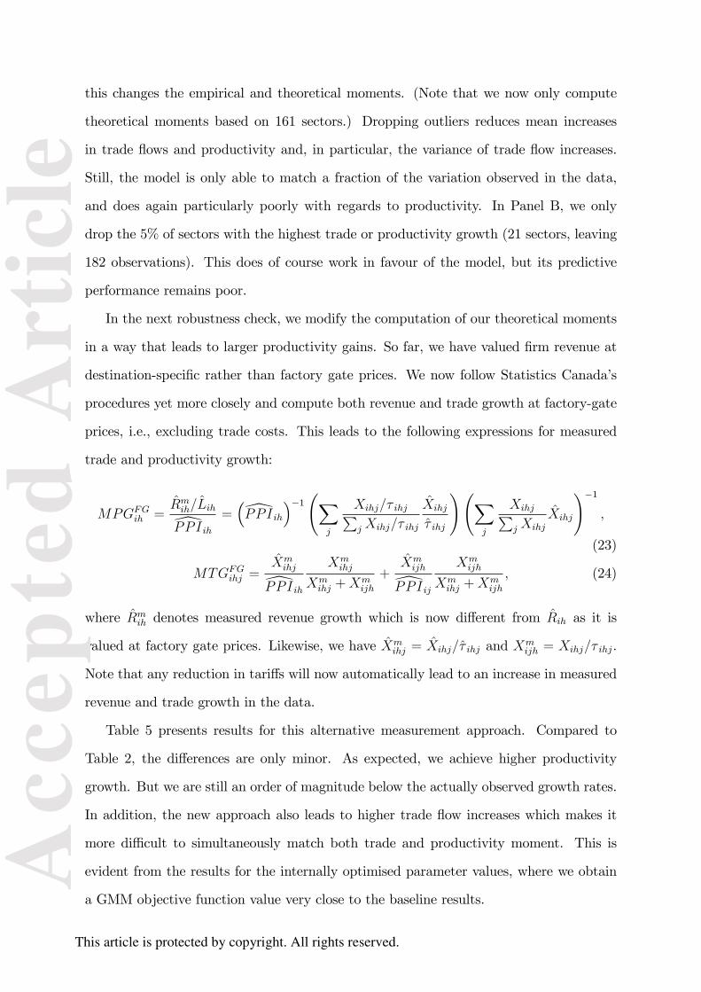
In the next robustness check, we modify the computation of our theoretical moments
in a way that leads to larger productivity gains. So far, we have valued firm revenue at
destination-specific rather than factory gate prices. We now follow Statistics Canada’s
procedures yet more closely and compute both revenue and trade growth at factory-gate
prices, i.e., excluding trade costs. This leads to the following expressions for measured
trade and productivity growth:
MPGFGih =
Rmih/Lih
PP I ih=(PP I ih
)−1(∑
j
Xihj/τ ihj∑j Xihj/τ ihj
Xihj
τ ihj
)(∑j
Xihj∑j Xihj
Xihj
)−1
,
(23)
MTGFGihj =
Xmihj
PP I ih
Xmihj
Xmihj +Xm
ijh
+Xmijh
PP I ij
Xmijh
Xmihj +Xm
ijh
, (24)
where Rmih denotes measured revenue growth which is now different from Rih as it is
valued at factory gate prices. Likewise, we have Xmihj = Xihj/τ ihj and Xm
ijh = Xihj/τ ihj.
Note that any reduction in tariffs will now automatically lead to an increase in measured
revenue and trade growth in the data.
Table 5 presents results for this alternative measurement approach. Compared to
Table 2, the differences are only minor. As expected, we achieve higher productivity
growth. But we are still an order of magnitude below the actually observed growth rates.
In addition, the new approach also leads to higher trade flow increases which makes it
more diffi cult to simultaneously match both trade and productivity moment. This is
evident from the results for the internally optimised parameter values, where we obtain
a GMM objective function value very close to the baseline results.
This article is protected by copyright. All rights reserved.
Acc
epte
d A
rtic
le

Our final robustness check in this section uses a different modelling of tariffs. So
far, we have followed the approach in most of the literature of treating tariffs as being
isomorphic to physical transportation costs in our formulation of overall trade costs (see
Section 3.1). We now explicitly model tariffs as a payment deducted from the firm’s
revenue. This brings about a number of changes to the equilibrium conditions of our
model. We briefly outline the most important ones here and refer the reader to Appendix
C for a full exposition of the modified model.
Most importantly, the firm’s market-specific profit function can now be written as:
πihj =pihj
1 + tihjqihj (pihj)− τ ihjqihj (pihj)
1
γ− fihj, (25)
where pihj denotes the price paid by the consumers of the importing country. This mod-
ification leads to the following equilibrium conditions for price indices and productivity
cut-offs (expressed in changes):
Pij =
[∑h
TihjXihj∑h TihjXihj
(Tihj
)1− σiσi−1
aiγ
]−1/aiγ
, (26)
γ∗ihj =
(Tihj
) σiσi−1
Pij, (27)
where Tihj ≡ 1+tihj. Similar to before, we can use (26) to solve for price index changes as
a function of tariff changes. Using (27) we can then solve for changes in the productivity
cut-offs. These are suffi cient to calculate changes in trade flows and industry revenues:
Xihj = Nihj =(γ∗ihj)−aiγ , (28)
Rih = Πih = Lih =∑j
Xihj∑j Xihj
Xihj. (29)
Note that for the purpose of our estimation, the key change is that the parameter σi
now enters the price index and productivity cut-off equilibrium conditions. Given that
we noted before that the impact of variations in σi on the theoretical moments was
This article is protected by copyright. All rights reserved.
Acc
epte
d A
rtic
le

quantitatively unimportant in our baseline model, this modification should, in principle,
allow the model to match the data better. This is because σi now directly enters the
productivity cut-offs (and thus nominal trade flow increases), rather than only entering
measured trade and productivity growth through the theoretical PPI.
In practice, however, this additional impact channel only leads to minor improvements
in the model’s predictive performance, as is evident from Table 6. The reason for this is
that aiγ and 1/σi tend to move our moments in the same directions. Thus, the increased
impact σi now has is not useful in matching the data. Figure 3 illustrates this by plotting
deviations of theoretical from empirical moments against aiγ and σi, as Figure 2 did for
our baseline model. We note that the tendency to move theoretical moments in similar
ways also explains the reduction in the precision with which the parameter aiγ is now
estimated (although σi is now of course estimated with a lower standard error).31
Robustness Checks II: Is Our Baseline Model Too Stylized?
We now return to the issue of whether our baseline model abstracts from too many real-
world features to make a comparison with the data informative. We argued in Section
2 that several aspects of CUSFTA made it a reasonable abstraction to rely on models
with relatively simple, tariff-reduction-driven data generating processes. Nevertheless,
an important concern is that the observed post-1988 changes in trade and productivity
are simply too large to be explained by tariff reductions alone, and that other factors
must have been present in the process generating the observed data. Since such factors
are absent from our model, one might not be surprised that the model falls short of
generating suffi cient trade and productivity responses. We try to address this concern in
several ways in this subsection.
We start by progressively removing sources of variation from the data which are
arguably absent from the model. First, we take first differences in growth rates between
the post- and pre-liberalisation period (1980-1988 and 1988-1996, respectively). The
31In an additional robustness check (not reported), we also constructed a PPI deflator by giving equalweight to all active firms, rather than overweighting larger firms (see Appendix A for details). Thisyielded very similar results to the one in Table 2, with a GMM objective function value of 91.9835compared to 91.7885 for the baseline model.
This article is protected by copyright. All rights reserved.
Acc
epte
d A
rtic
le

purpose of this exercise is to eliminate time-invariant factors from the data which are
absent from our model, such as technological progress leading to ongoing productivity
growth. Indeed, first-differenced growth rates are less than half as large on average as
growth rates in levels (see Table 7, first line). To assure comparability with these ‘cleaned’
data and our theoretical predictions, we perform a similar procedure when generating
data from our model. That is, we separately calculate predictions for the pre- and the
post-liberalization period in the same way described above for our baseline model. For
the 1980-1988 period, we use initial trade flows for 1980 and observed tariff cuts between
1980 and 1988. (The remaining parameters, aγ and σ, are assumed to remain constant
over the entire period 1980-1996.) We then first-difference the generated data across the
two periods in the same way we differenced the actual data.32
Secondly, we implement a difference-in-differences strategy similar to Trefler (2004).
We regress first differences of trade and productivity growth (as calculated above) on first
differences in tariff cuts, and compute predicted values from these two regressions. We
then use the model to generate data for both the pre- and post-liberalization period (as
described above) and run the same regressions on the generated data. We again compute
predicted values and compare them to the predicted values from the regressions using the
actual data. The purpose of this approach is to only use variation which is correlated with
tariff cuts. Since this is the driving force in the model’s data generating process, we would
expect the model to perform much better when focusing on this source of variation only.
The first line of Table 8 shows that this approach does indeed lead to further substantial
reductions in empirical mean growth rates, especially for productivity.
Table 7 presents the full results for first differences, Table 8 for the difference-in-
differences approach. As discussed, first-differencing the data reduces the magnitude of
all moments with the exception of the variance of (first-differenced) productivity growth
rates. However, the first-differenced theoretical moments are also smaller, so that we only
32An alternative approach would be to directly compare the 1988-1996 model predictions to the first-differenced data. This is not strictly correct, however, because there were small (GATT-driven) tariffreductions in the 1980-1988 period, too. These generate positive, if small, growth in trade and pro-ductivity in our model, which in turn lead to differences between first-differenced and 1988-1996 modelgrowth rates. In practice, however, results are very similar for this alternative approach (available fromthe authors).
This article is protected by copyright. All rights reserved.
Acc
epte
d A
rtic
le

obtain a small reduction in the percentage difference with the first two empirical moments
(mean growth rates). The reduction in the covariance difference is more substantial, but
differences in variances actually go up slightly. Thus, the model’s overall performance is
similar to our baseline results. This is true when we use externally estimated data (row
2) and when we choose parameters to match the empirical moments (rows 3-4). This lack
of improvement is also reflected in the GMM objective function value which is basically
unchanged compared to the baseline results in Table 2.
The difference-in-differences approach fares better. We now get much closer to ob-
served trade flow changes even when using externally estimated parameters (we match
75% of the mean increase and 50% of the variance). We also do better for mean pro-
ductivity increases (we match 30% of the observed increase). However, we are still an
order of magnitude below the actual variance of productivity increases and the covariance
between trade and productivity increases. The better ability of the model to match the
‘cleaned’data is also reflected in a lower GMM objective function value, although we still
reject the null that the moment restrictions implied by our model are valid at the 1%
level.
A remaining concern is that tariff reductions might be correlated with other factors
present in the data, but absent from our model. As discussed in Section 2, there are
a priori few reasons to believe that such omitted variables were important during the
implementation of CUSFTA. We also have econometric evidence from Trefler (2004) that
endogeneity issues related to tariff reductions are unlikely to be a major problem in our
data (see Section 2). Nevertheless, we explore possible implications for our results in
the following. A natural candidate for an omitted variable are changes in other trade
costs which we assumed to be constant in our baseline simulation. These changes could
be due to reductions in non-tariff barriers (including more effi cient border procedures),
reductions in physical transport costs over the sample period, or even a reduction in
the uncertainty regarding possible future tariff hikes.33 If such variables were indeed
important, using only the variation in the data associated with tariff cuts is still not a
33See footnote 10 for details.
This article is protected by copyright. All rights reserved.
Acc
epte
d A
rtic
le

‘fair’comparison because part of this variation will still be driven by factors not present
in the model.
It is easy to show, however, that allowing for such correlations is not suffi cient to
rescue our model. In Section 3, we defined trade costs as consisting of a tariff (thj) and a
component comprising all other trade costs (chj), such that τhj = (1 + chj) (1 + thj). We
do not observe changes in (1 + chj) but can make a number of assumptions which should,
in principle, help the model to generate larger trade and productivity gains. Our first
approach is to work with sectorial-level estimates of a and σ as before and assume that
the change in (1 + cCAN,US) and (1 + cUS,CAN) is proportional to observed reductions
of US and Canadian import tariffs, respectively. That is, for h, j ∈ CAN,US, we
assume that(1 + c
′hj
)/ (1 + chj) = c
(1 + t
′hj
)/ (1 + thj). The change in τhj will thus be
τhj = c[(
1 + t′hj
)/ (1 + thj)
]2.34 The second approach uses our GMM framework but
allows for a third parameter in addition to aγ and σ —mean changes in (1 + chj). That
is, c =(1 + c
′hj
)/ (1 + chj) and τhj = c
(1 + t
′hj
)/ (1 + thj). We now try to minimize our
GMM objective function through varying aγ, σ and c. Note that the first approach, in
particular, is similar in spirit to our previous robustness check of varying σ and ar by
factors which are common across sectors.35
Table 9 presents the results for both robustness checks. In lines 2-4, we show the-
oretical moments for different values of c. Lines 2 and 3 use values of c which lead to
theoretical predictions of mean trade growth rates which are too low and too high, re-
spectively. As expected, decreases in c (i.e., stronger reductions in other trade costs) lead
to higher trade and productivity growth. Line 4 uses c = 0.98 which allows us to exactly
match mean trade growth. At this value, however, we overestimate the variance of trade
growth by a factor of five, but still only achieve less than one eight of the observed mean
productivity growth, and only one hundredth of the variance of productivity growth. Line
34We assume that trade costs other than tariffs for exports and imports to and from the rest of the worldremain unchanged. Allowing for less than perfect correlation between chj and thj is also possible butdoes not change the following results qualitatively. Note that if chj and thj are completely uncorrelated,our previous approach of using tariff-cut related variation will again be valid.35Again, we restrict the variation in chj to be governed by one additional parameter only. As discussed
in footnote 27, allowing for more flexibility would make our model underidentified and our approach muchless meaningful.
This article is protected by copyright. All rights reserved.
Acc
epte
d A
rtic
le

5 shows moment deviations for our first-step GMM estimates. While we now vary aγ, σ
and c, we do not see major improvements as compared to our baseline GMM results in
Table 2.
The intuition for these negative results is similar in all cases. Allowing for changes in
non-tariff trade costs only allows the model to generate larger increases in both trade and
productivity; it does nothing to help address the model’s problem of getting the relative
growth rates right. This holds true even when we vary aγ, σ and c simultaneously because
a and c have similar impacts on our theoretical moments and do not allow the model to
generate suffi cient variation in trade and productivity growth.
The effects are more subtle for the full GMM estimation. As before, the presence of
our weighting matrix W optn implies that the estimation now places much less weight on
the trade moments, and in particular on the deviation from the variance of trade growth
across sectors. This somewhat alleviates the problem that increases in c cannot generate
enough productivity growth because of the implied deviation from the trade growth
variance. As a result, we obtain much lower values for the GMM objective function than
in our baseline estimation. However, from a statistical point of view the model is still
rejected at the 1%-level. We also note that the parameter estimates are quite extreme.
We find very low estimates for aγ and σ, and an implied reduction in non-tariff trade
costs (1 + chj) of more than 50%. This does not seem plausible given the absence of
major changes in transportation technology over the sample period and the rather minor
reductions in non-tariff barrier agreed to in CUSFTA.
One final possibility is that there are factors present in the data, but absent from the
model, which lead to increases in productivity, but not trade growth, and happen to be
correlated with tariff reductions over the sample period. We cannot definitely exclude
this possibility because we do not see a way of ‘cleaning’our data of such factors that
is compatible with our theoretical framework.36 We note, however, that the solution we
will eventually propose relies on a related mechanism. As we show below, one way of
36Trefler (2004) controls for productivity trends in the US and includes business cycle controls based onaggregate movements in GDP and exchange rates. We did not adopt this approach because our modelpredicts that such variables would themselves depend on CUSFTA-induced tariff reductions, makingthem unsuitable as controls.
This article is protected by copyright. All rights reserved.
Acc
epte
d A
rtic
le
matching model predictions and data is to allow for sources of within-firm productivity
growth which are triggered by tariff reductions.
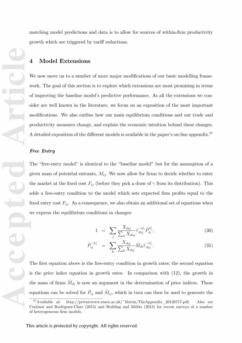
4 Model Extensions
We now move on to a number of more major modifications of our basic modelling frame-
work. The goal of this section is to explore which extensions are most promising in terms
of improving the baseline model’s predictive performance. As all the extensions we con-
sider are well known in the literature, we focus on an exposition of the most important
modifications. We also outline how our main equilibrium conditions and our trade and
productivity measures change, and explain the economic intuition behind these changes.
A detailed exposition of the different models is available in the paper’s on-line appendix.37
Free Entry
The “free-entry model”is identical to the “baseline model”but for the assumption of a
given mass of potential entrants, Mij. We now allow for firms to decide whether to enter
the market at the fixed cost Fij (before they pick a draw of γ from its distribution). This
adds a free-entry condition to the model which sets expected firm profits equal to the
fixed entry cost Fij. As a consequence, we also obtain an additional set of equations when
we express the equilibrium conditions in changes:
1 =∑j
Xihj∑nXihn
τ−aiγihj P
aiγij , (30)
P−aiγij =
∑h
Xihj∑hXihj
Mihτ−aiγihj . (31)
The first equation above is the free-entry condition in growth rates; the second equation
is the price index equation in growth rates. In comparison with (12), the growth in
the mass of firms Mih is now an argument in the determination of price indices. These
equations can be solved for Pij and Mij, which in turn can then be used to generate the
37Available at: http://privatewww.essex.ac.uk/~hbrein/TheAppendix_20130717.pdf. Also seeCostinot and Rodriguez-Clare (2013) and Redding and Melitz (2013) for recent surveys of a numberof heterogeneous firm models.
This article is protected by copyright. All rights reserved.
Acc
epte
d A
rtic
le

model’s predictions for all other variables of interest.
Adding free entry implies an additional effect of trade liberalization on industry pro-
ductivity and trade flows, as the mass Mij reacts to changes in tariff barriers, with a
decrease if import barriers fall and an increase if export barriers fall. Other things equal,
an increase in Mij leads to higher average productivity as low-productivity entrants de-
cide not to produce. Similarly, an increase (decrease) in Mij increases (decreases) the
number of exporters and leads, ceteris paribus, to more (less) exports.
Thus, allowing for free entry has an a priori ambiguous effect on trade flows, as well
as on theoretical and (through changes in the PPI) measured productivity. Whether
we observe an overall increase depends on whether the effect of lower US import tariffs
(which raises MCAN) outweighs the effect of lower Canadian import tariffs (which lowers
MCAN). This ambiguity is reflected in the results in Table 10, where we actually observe a
slightly lower increase in average Canadian productivity when using externally estimated
parameter values (row 2). Thus, allowing for free entry does not help with improving
the model’s predictive performance with regards to productivity. We do predict slightly
higher trade flow increases, but remain far off our target of 118%.38
The fact that allowing for free entry only marginally affects model predictions also
explains that the free-entry model is not noticeably better than the baseline model at
matching our empirical moments when we can choose parameter values optimally (rows 3-
4). Indeed, the GMM objective function value is only slightly lower than the one reported
in Table 2 (83.30 compared to 91.79).
General Equilibrium
In our second model extension, we replace the quasi-linear utility function of the baseline
model with a Cobb-Douglas utility function
Uj =∏i∈I
(Qij)µij , (32)
38Note that changes in trade flows are influenced by changes in both MUS and MCanada Thus, tradeand productivity growth need not move in the same direction as compared to the baseline model.
This article is protected by copyright. All rights reserved.
Acc
epte
d A
rtic
le

where µij > 0,∑
i µij = 1. We also assume free entry and remove the numéraire sector.39
In analytical terms, the most important changes implied by this model are (i) the
presence of wages both as unknowns and as a relevant variable in many of the equations
that pin down industry outcomes; (ii) the presence of labour market clearing within the
equilibrium conditions. For the sake of brevity, we omit a detailed description of the
equilibrium conditions in growths rates here. In the On-line Appendix we show that we
can obtain predictions for all growth rates of interest by manipulating the growth rates
of the price index, the free-entry condition and the labour market clearing condition.40
In this general equilibrium version of our model, the effects of trade liberalization now
also operate via changes in the demand for labour and its subsequent effect on wages.
A lowering of US import tariffs leads to a higher demand for Canadian exports, which
in turn raises Canadian labour demand and (with a fixed labour supply) wages. Ceteris
paribus, this increases production costs, dampening the overall increase in Canadian
exports but also driving some of the less productive Canadian firms out of the market.
A reduction in Canadian import tariffs has the opposite effect through a reduction in
domestic demand for Canadian producers. Compared to the baseline model, this lowers
wages and production costs, dampening the productivity increasing effect of tougher
import competition from the US.
Note that these wage effects operate in addition to the free-entry effects described in
the last subsection, but also modify them. For example, a reduction in Canadian wages
in response to lower Canadian import tariffs will also dampen the decline in the number
of potential entrants (Mij). Thus, Canadian exports will decline by less compared to a
39Allowing for free entry and Cobb-Douglas preferences while keeping the numéraire sector (that is,fixing all wages to 1) yields results identical to those of our “free-entry” model. This is due to thefact that, besides labor income being the same across the two models, the free-entry conditions in bothmodels lead to the same price levels.40Ossa (2014) points out that the choice of numéraire matters in the presence of aggregate trade
imbalances. This is not an issue for our models with quasi-linear preferences because aggregate tradedeficits are absorbed by our homogeneous final goodA; but it is relevant for the present general equilbriumextension. Ossa suggests adjusting the raw data to eliminate trade imbalances. Unfortunately, it isunclear how to extend his procedure to labor productivity, our second key data input. It also seemslikely that cleaning our trade data as suggested by Ossa would not change our results qualitatively.This is because our empirical moment, total trade growth (export plus imports), would basically remainunchanged. Trade flows also influence model predictions through initial trade shares, but they do nothave a quantitatively important influence on the relative growth rate of trade and productivity (see thediscussion on pp. 14-15).
This article is protected by copyright. All rights reserved.
Acc
epte
d A
rtic
le

situation without a wage response, and productivity will drop by less.
A priori, the expected change in our model predictions is thus again ambiguous com-
pared to both the baseline and the free-entry version of our model. Table 11 shows that
trade and productivity growth are indeed very similar to the free-entry version when we
use externally estimated parameter values (row 2). The same is true when we choose
parameter values to match our empirical moments. Our key statistic, the GMM objective
function value is practically identical to the one for the free-entry version. We conclude
that allowing for general equilibrium wage effects is quantitatively unimportant in match-
ing the data.
Intermediate Inputs
In the third extension of our model, we assume that the production of manufacturing
varieties requires both labour and intermediate inputs:
qij (γ) = γ
[Qinputij (γ)
αi
]αi [lij (γ)
1− αi
]1−αi, (33)
where Qinputij denotes the amount of the aggregate manufacturing good used as an inter-
mediate input, and αi ∈ [0, 1).41
In this case, the price and expenditure equations in changes can be rewritten as
Paiγσi−1ij =
(Eij
)σi−aiγ−1(1−σi)
2
[∑h
Xihj∑mXimj
τ−aiγihj
1
Pαiaiγih
] 11−σi
, (34)
Eij =1
Eij
[mij + PijQ
inputij P
−aiγαiij
(∑h
Xijh∑hXijh
τ−aiγijh P
aiγih E
aiγσi−1ih
)]. (35)
This yields a system of non-linear equations in Pij and Eij. Once we solve for Pij and Eij,
we can solve for the growth rates of the variables of interest. The expression for expendi-
ture is more elaborate now because it now also encompasses purchases of intermediates
(i.e., Eij = mij + PijQinputij ).
41For simplicity, we abstract from interindustry input-output linkages (see Caliendo and Parro, 2012,for such an extension). Note that in order to isolate the effect of allowing for intermediates, we have alsoswitched back to the no free-entry, no general equilibrium case.
This article is protected by copyright. All rights reserved.
Acc
epte
d A
rtic
le

Labour productivity is now value added per worker,
V AijLij
=Rij − PijQv
ij
Lij, (36)
and its measured growth rate is
MPGintih =
V Aih/LihPP I ih
=(Pij
)−αi(γ′ih/γih) . (37)
A comparison with expressions (14) and (18) reveals that allowing for intermediate in-
puts adds(Pij
)−αias an additional source of measured productivity growth. Intuitively,
the availability of cheaper (imported) intermediate inputs leads to a stronger decrease in
the domestic PPI for a given change in the productivity of the ‘average’firm (γ′ih/γih),
and thus to stronger increases in measured productivity. Note, however, that increases
in γ′ih/γih will tend to be lower than in the baseline model. This is because lower input
costs mean that some of the less productive firms can stay in the market, ceteris paribus.
Table 12 shows that the overall impact on productivity is positive. When we use ex-
ternally estimated parameter values (row 2), we more than double predicted productivity
growth as compared to the baseline model. However, a large gap between predicted and
actual productivity gains remains (2.95% vs. 30.41%). The results also reveal that allow-
ing for intermediates increases predicted trade flows as intermediates make up a growing
proportion of international trade. Thus, while the presence of intermediate inputs allows
us to obtain larger productivity increases, it also leads to stronger trade growth. This
again makes it diffi cult for the model to simultaneously match trade and productivity
growth and explains why our GMM approach is still unsuccessful in matching the empir-
ical moments (rows 3 and 4). While the GMM objective function is 50% lower than in
the baseline model, the overidentification test still rejects at the 1%-level.42
42Note that the model with intermediates has one additional parameter (α), so that we lose one degreeof freedom as compared to the baseline model. This is taken into account in the reported p-value whichin any case is substantially below the 1% level.
This article is protected by copyright. All rights reserved.
Acc
epte
d A
rtic
le

Multi-product Firms
The final extension we consider is to introduce multi-product firm features as modelled
in Bernard et al. (2011) into the baseline model.43 As in Bernard et al. (2011), we
introduce an additional layer into our utility function by modelling final goods (Qi) as a
continuum of products which are imperfect substitutes in demand. Within each product,
firms supply horizontally differentiated varieties. While firms produce one variety of each
product, they can supply a range of products. In addition to productivity (γ), firms now
also draw ‘product attributes’(λ) for the continuum of products which act as demand
shifters. We assume that λ is Pareto distributed with location parameter kλ and shape
parameter aλ. Firms observe their γ and λ and decide whether to pay the additional fixed
costs associated with entering different markets and products. As we explain in the On-
line Appendix, the derivation of our equilibrium conditions and productivity measures
is similar to the baseline model. The main difference is that they now contain a third
parameter (aλ) which governs productivity and trade growth rates in addition to aγ and
χ.44
Intuitively, the “multi-product model”reinforces the between-firm reallocation effect
on productivity with a within-firm reallocation effect as a response to trade liberalization.
Firms reallocate resources from product-varieties with (now loss-making) low attributes
to product-varieties with (more profitable) high attributes, thus leading to higher firm-
level productivity. As we show in the On-line Appendix, this leads to a stronger decrease
in the industry PPI and thus a more pronounced increase in industry productivity. At
the same time, the additional within-firm productivity effect also reduces the increase in
imports as domestic firms become more productive relative to foreign exporters.
As seen in Table 13, this combination of effects makes the multi-product firm model
quite successful in matching the observed data. We are now able to simultaneously match
productivity and trade flow increases by choosing the appropriate model parameters.45
43Apart from the multi-product firm features described below, we thus switch back to the assumptionsof the benchmark model. That is, we assume a given massMij , impose αi = 0 for all sectors, and assumequasilinear preferences and the presence of a numéraire good.44χ governs the substitutability of product varieties and is the equivalent of σ in our baseline model
in terms of its role in the estimation procedure.45Note that we do not have estimates for our parameters obtained from external sources. This would
This article is protected by copyright. All rights reserved.
Acc
epte
d A
rtic
le

Indeed, our overidentification test is now unable to reject the model at conventional
levels of statistical significance.46 We see this as an indication that sources of within-
firm productivity increases need to be added to our baseline model in order to solve the
problem of simultaneously matching trade and productivity growth rates in the wake of
CUSFTA. While we have used the multi-product firm model of Bernard et al. (2011)
to achieve these within-firm productivity gains, our conjecture is that other modelling
frameworks will yield similar results. For example, within-firm productivity gains could
also be achieved through technological upgrading in response to trade liberalization (see
Bustos (2011)). As we noted in the introduction to this paper, the presence of within-
firm productivity effects has indeed been documented for CUSFTA by Trefler (2004) and
Lileeva and Trefler (2011). But there is evidence that such effects were important in
other trade liberalization episodes as well, including Argentina (see Bustos, 2011) and
India (see Topalova and Khandelwal, 2011).
One concern with the multi-product extension is that we have now one more parameter
at our disposition. This will make it easier to match our empirical moments within a
given sample, but might not necessarily lead to the best out-of-sample predictions (this
is the classic ‘overfitting’problem).
In order to evaluate whether this is an issue in the present context, we also perform
the following out-of-sample test of our baseline model and the four extensions discussed
above. We first estimate the model parameters on the pre-liberalisation period (1980-
1988). We then use these estimates to obtain trade and productivity growth predictions
for the post-liberalization period (1988-1996) and recompute the GMM objective function
with these new predictions.47 If overfitting were a problem, we would expect a higher
value for the multi-product firm model than for the other extensions. Table 14 shows
that this is not the case —the multi-product firm model continues to outperform all other
extensions.
require firm-level data similar to the data available to Bernard et al. (2011). Unfortunately, we do nothave access to such data for Canada or the US.46Note that the p-value in Table 13 has been adjusted to account for the loss of one degree of freedom
due to the fact that now have three parameters.47To ensure comparability, we use the same weighting matrix as in the original (post-liberalization)
GMM estimation.
This article is protected by copyright. All rights reserved.
Acc
epte
d A
rtic
le
5 Conclusions
In this paper, we examined the quantitative predictions of heterogeneous firm models à
la Melitz (2003) in the context of the Canada - US Free Trade Agreement (CUSFTA) of
1989. We computed predicted increases in trade flows and measured productivity across
a range of standard models and compared them to the post-CUSFTA increases observed
in the data.
Starting from a version of Chaney (2008), we found that this model was not able
to simultaneously match both trade and productivity increases. This was true when we
used sectorial parameter estimates obtained from other data sources, or when we chose
parameters to minimize deviations between theoretical and empirical moments via a
simple GMM procedure. Our basic result were also robust to different ways of computing
predicted productivity and trade growth, and to comparing model predictions and data
in ways which eliminate a number of unmodelled determinants of trade and productivity
increases. In each case, the fundamental problem remained that predicted increases in
trade flows for a given change in tariffs were much too large relative to the predicted
increase in measured productivity.
We also considered different extensions of our basic framework by allowing for free
entry, tradable intermediate inputs, general equilibrium effects operating through wages,
and endogenous firm-level productivity through adjustments in product scope as in
Bernard et al. (2011). Free entry and general equilibrium effects did not markedly
improve the model’s performance. Introducing tradable intermediates helped somewhat,
but formal over-identification tests in our GMM framework still rejected this model vari-
ant. The only model that is capable of providing a good fit to the data and of passing
our over-identification tests was the multi-product firm extension. We interpret these
results as evidence for the need to explicitly model within-firm productivity increases
when constructing quantitative trade models capable of explaining first-order features of
trade liberalization episodes.
Holger Breinlich, University of Essex, CEP and CEPR
This article is protected by copyright. All rights reserved.
Acc
epte
d A
rtic
le

Alejandro Cuñat, University of Vienna and CES-ifo
References
[1] Alvarez, F. and Lucas, R.E. (2007). ‘General equilibrium analysis of the Eaton—Kortum model of international trade’, Journal of Monetary Economics, vol. 54, pp.1726—1768.
[2] Arkolakis, C., Costinot, A. and Rodríguez-Clare, A. (2012). ‘New trade models, sameold gains?’American Economic Review, vol. 102(1), pp. 94—130.
[3] Armenter, R. and Koren, M. (2014). ‘Economies of scale and the size of exporters’,Journal of the European Economics Association, forthcoming.
[4] Balistreri, E., Hillberry, R. and Rutherford, T. (2011). ‘Structural estimation andsolution of international trade models with heterogeneous firms’, Journal of Inter-national Economics, vol. 83(2), pp. 95—108.
[5] Bernard, A.B., Eaton, J. Jensen, J.B. and Kortum, S. (2003). ‘Plants and produc-tivity in international trade’, American Economic Review, vol. 93(4), pp. 1268-1290.
[6] Bernard, A.B., Redding, S.J. and Schott, P.K. (2011). ‘Multi-product firms and tradeliberalization’, Quarterly Journal of Economics, vol. 126(3), pp. 1271-1318.
[7] Breinlich, H. (2008). ‘Trade liberalization and industrial restructuring through merg-ers and acquisitions’, Journal of International Economics, vol. 76(2), pp. 254-266.
[8] Broda, C. and Weinstein, D.E. (2006). ‘Globalization and the gains from variety’,Quarterly Journal of Economics, vol. 121(2), pp. 541-585.
[9] Burstein, A. and Cravino, J. (2014). ‘Measured aggregate gains from internationaltrade’, American Economic Journal - Macroeconomics, forthcoming.
[10] Bustos, P. (2011). ‘Trade liberalization, exports, and technology upgrading: evidenceon the impact of MERCOSUR on Argentinian firms’, American Economic Review,vol. 101(1), pp. 304—340.
[11] Caliendo, L. and Parro, F. (2012). ‘Estimates of the trade and welfare effects ofNAFTA’, Working Paper no. 18508, NBER.
[12] Chaney, T. (2008). ‘Distorted gravity: the intensive and extensive margins of inter-national trade’, American Economic Review, vol. 98(4), pp. 1707-1721.
[13] Canada-United States Free Trade Agreement, http://www.worldtradelaw.net/nafta/CUSFTA.pdf(last accessed 10 February 2013).
[14] Corcos, G., del Gatto, M., Mion, G. and Ottaviano, G.I. (2011). ‘Productivity andfirm selection: quantifying the “new”gains from trade’, The Economic Journal, vol.122(561), pp. 754-798.
This article is protected by copyright. All rights reserved.
Acc
epte
d A
rtic
le

[15] Costinot, A. and Rodríguez-Clare, A. (2013). ‘Trade theory with numbers: quanti-fying the consequences of globalization’, in (Gopinah, G., Helpman, E. and Rogoff,K., eds.), Handbook of International Economics, vol. 4, Elsevier, forthcoming.
[16] Dekle, R., Eaton, J. and Kortum, S. (2008). ‘Global rebalancing with gravity: mea-suring the burden of adjustment’, Working Paper no. 13846, NBER.
[17] Eaton, J. and Kortum,S. (2002). ‘Technology, geography, and trade’, Econometrica,vol. 70(5), pp. 1741-1779.
[18] Eaton, J., Kortum S. and Kramarz, F. (2011). ‘An anatomy of international trade:evidence from French firms’, Econometrica, vol. 79(5), pp. 1453-1498.
[19] Friedman, M. (1953). Essays in Positive Economics. Part I - The Methodology ofPositive Economics, Chicago: Chicago University Press.
[20] Frizzell, A., Pammett, J., and Westell, A. (1989). The Canadian General Election of1988, Ottawa: Carleton University Press.
[21] Ghironi, F. and Melitz, M.J. (2005). ‘International trade and macroeconomic dy-namics with heterogeneous firms’, Quarterly Journal of Economics, vol. 120(3), pp.865-915.
[22] Greene, W. (2000). Econometric Analysis, 4th edition, Upper Saddle River: PrenticeHall International.
[23] Head, K. and Ries, J. (1999) ‘Rationalization effects of tariff reductions’, Journal ofInternational Economics, vol. 47(2), pp. 295-320.
[24] Head, K. and Ries, J. (2001). ‘Increasing returns versus national product differen-tiation as an explanation for the pattern of US-Canada trade’, American EconomicReview, vol. 91(4), pp. 858-876.
[25] Hsieh, C.T. and Ossa, R. (2011). ‘A global view of productivity growth in China andIndia’, NBER Working Paper no. 16778.
[26] Kehoe, T.J. (2005). ‘An evaluation of the performance of applied general equilibriummodels of the impact of NAFTA’, in (Kehoe, T.J., Srinivasan, T.N. and Whalley,J. eds.), Frontiers in Applied General Equilibrium Modeling: Essays in Honor ofHerbert Scarf, Cambridge: Cambridge University Press.
[27] Krugman, P.R. (1979). ‘Increasing returns, monopolistic competition, and interna-tional trade’, Journal of International Economics, vol. 9(4), pp. 469-479.
[28] Krugman, P.R. (1980). ‘Scale economies, product differentiation, and the pattern oftrade’, American Economic Review, vol. 70(5), pp. 950-959.
[29] Lawless, M. (2009). ‘Firm export dynamics and the geography of trade’, Journal ofInternational Economics, vol. 77(2), pp. 245-254.
[30] Levchenko, A. and Zhang, J. (2011). ‘The evolution of comparative advantage: mea-surement and welfare implications’, Working Paper no. 16806, NBER.
This article is protected by copyright. All rights reserved.
Acc
epte
d A
rtic
le

[31] Melitz, M.J. (2003). ‘The impact of trade on intra-industry reallocations and aggre-gate industry productivity’, Econometrica, vol. 71(6), pp. 1695-1725.
[32] Ossa, R. (2012). ‘Why trade matters after all’, Working Paper no. 18113, NBER.
[33] Ossa, R. (2014). ‘Trade wars and trade talks with data’, American Economic Review,forthcoming.
[34] Redding, S.J and Melitz, M.J. (2013). ‘Heterogeneous firms and trade’, in (Gopinah,G., Helpman, E. and Rogoff, K., eds.), Handbook of International Economics, vol. 4,Elsevier, forthcoming.
[35] Schott, P.K. (2010). ‘U.S. manufacturing exports and imports by SIC or NAICScategory and partner country, 1972 to 2005’, manuscript, Yale University.
[36] Statistics Canada (1991). ‘Industry price indexes, 1986 = 100’, Statistics Canada,catalogue no. 62-558.
[37] Statistics Canada (1993). ‘Gross domestic product by industry, 1992 = 100’, Statis-tics Canada, catalogue no. 15-512-XPB.
[38] Statistics Canada (2001). ‘A guide to deflating the input-output accounts: sourcesand methods’, Statistics Canada, catalogue no. 15F0077GIE.
[39] Statistics Canada (2012a). ‘The industrial product price index (IPPI)’,http://www.statcan.gc.ca (last accessed 15 April 2014).
[40] Statistics Canada (2012b). ‘Industry price indexes’, Statistics Canada, catalogue no.62-011-X.
[41] Topalova, P. and Khandelwal, A. (2011). ‘Trade liberalization and firm productivity:the case of India’, Review of Economics and Statistics, vol. 93(3), pp. 995-1009.
[42] Trefler, D. (2004). ‘The long and short of the Canada-U.S. free trade agreement’,American Economic Review, vol. 94(4), pp. 870-895.
[43] Wei, S.J. (1996). ‘Intra-national versus international trade: how stubborn are nationsin global integration?’,”Working Paper no. 5531, NBER.
This article is protected by copyright. All rights reserved.
Acc
epte
d A
rtic
le

Appendix
A PPI Deflators
In the following, we describe how Statistics Canada calculated producer price indices
(PPIs) during our sample period, which are used to convert current to constant prices
entries in our data. We then outline how we apply that procedure to the computation of
theoretical moments in our setting.48
During our sample period (1980-1996), Statistics Canada computed current price en-
tries for 243 industries of which 211 industries are in the manufacturing sector. For
manufacturing, there was also a more disaggregated commodity level, the so-called Prin-
cipal Commodity Group Aggregation (PCGA), for which prices and shipment values
were available. There were 1057 PCGAs in total which served as the starting point for
constructing deflators.
In a first step, Statistics Canada computed PCGA price indices via the following sam-
pling procedure. Each month, Statistics Canada obtained price quotes from important
producers and from a random sample of smaller producers of a given PCGA manufac-
turing product. From these quotes, an average price was calculated.49 Price quotes
were always based on so-called factory gate prices which excluded any costs associated
with transport, distribution, subsidies, taxes or tariffs. The particular weights used in
computing the average across price quotes varied from PCGA to PCGA, but generally
more weight was given to producers accounting for a larger fraction of industry output.
Yearly average prices were then computed as arithmetic averages over the 12 monthly
average prices. The sample of firms used for obtaining price quotes was updated every
December. That is, Statistics Canada drew a new sample of smaller producers from the
currently active firms. If any producer went out of business or dropped a product, Sta-
tistics Canada chose a still active producer/product as a replacement. By construction
48The following is based on Statistics Canada (1991; 1993; 2001; 2012a; 2012b).49The exact number of price quotes obtained varied slightly over time. Currently, 3 to 15 price quotes
are obtained for each PCGA. This number was slightly smaller in the earlier parts of our sample periodbut the basic methodology described in the following did not change substantially (see Statistics Canada,2001, 2012a).
This article is protected by copyright. All rights reserved.
Acc
epte
d A
rtic
le

(and by necessity), the sample from which price quotes were obtained was thus based on
the set of currently active firms. In a second step, Statistics Canada combined PCGA
price indices into industry-level PPIs using current shipment values as weights.50 The
number of PCGAs indices used as inputs varied across industries but was generally low,
at around 4-5 PCGAs per industry.
The choice of an appropriate deflator in the computation of our theoretical moments
depends on what we consider the most appropriate counterpart in the data to the ‘indus-
tries’in the model. In the data, an industry at the level of aggregation we are working at
comprises on average only 4-5 PCGAs. In contrast, there were around 40,000 establish-
ments in Canadian manufacturing in 1988, or around 200 per industry. This means that
each PCGA product will be produced by dozens or even hundreds of producers. Thus,
it seems appropriate to associate product varieties in our model with varieties of PCGA
products in the data (with each firm producing one variety of a PCGA product). For
the multi-product firm version of our model, it would seem natural to associate products
with PCGAs and product varieties with PCGA varieties.
Hence, if we associate model varieties with PCGA product varieties, our theoretical
PPI should be calculated following the random sampling procedure outlined above. That
is, we calculate an average price in each period based on a set of active domestic producers
in the period. As discussed, the way in which individual price quotes are weighted varies
by PCGA, but generally gives more weight to producers with larger market shares.
Thus, we compute a theoretical PPI which captures these features while preserving a
tight link to theoretical productivity. Specifically, we use the factory gate price charged
by the firm with average productivity, p (γih) = [σi/ (σi − 1)]wh/γih, where
γih =
[∑j
Nihj∑j Nihj
(γihj)σi−1
] 1σi−1
(A.1)
50Note that Statistics Canada did not use chain price indices during our sample period. This seemsto be different from current methods used in other countries such as the United States (see StatisticsCanada, 2001; Burstein and Cravino, 2014).
This article is protected by copyright. All rights reserved.
Acc
epte
d A
rtic
le

and
γihj =1
1−Gih
(γ∗ihj)∫ ∞
γ∗ihj
γσi−1gih (γ) dγ =
(aiγ
aiγ − σi + 1
) 1σi−1
γ∗ihj. (A.2)
As noted by Melitz (2003), γihj can be interpreted as a weighted average of firm pro-
ductivities, where the weights reflect the relative output shares of firms. Also note that
γihj is calculated as an average across active firms, reflecting the sampling procedure of
Statistics Canada. Thus,p′ihpih
=p (γih)
p (γ′ih)=γ′ihγih
, (A.3)
where
γ′ihγih
=
[∑
j
(N ′ihjNihj
Nihj∑j′ Nihj′
)]−1∑j
[N ′ihjNihj
(γ′ihjγihj
)σi−1Nihj
(γihj)σi−1∑
j′ Nihj′(γihj′
)σi−1
]1
σi−1
.
(A.4)
We do not have data for Nihj, but under the assumption that entry costs are proportional
to some observable destination-specific factor that is exogenous to the model (such as mij
in our baseline model):
Nihj∑j Nihj
=Xihj/
(aiγσi
aiγ−σi+1
)Fihj∑
j Xihj/(
aiγσiaiγ−σi+1
)Fihj
=Xihj/mij∑j Xihj/mij
. (A.5)
From (8) and Nihj =(kih/γ
∗ihj
)aiγ Mih,
γihj =
(aiγ
aiγ − σi + 1
) 1σi−1
γ∗ihj =
(aiγ
aiγ − σi + 1
) 1σi−1
kih (Mih)1
aiγ N− 1
aiγ
ihj . (A.6)
We can approximate
Nihj
(γihj)σi−1∑
j′ Nihj′(γihj′
)σi−1 =(Xihj/mij)
1−σi+aiγ
aiγ∑j′ (Xihj′/mij′)
1−σi+aiγaiγ
. (A.7)
In an (unreported) robustness check, we also experimented with giving equal weight
to the prices charged by active firms. This means that changes in the PPI are not affected
This article is protected by copyright. All rights reserved.
Acc
epte
d A
rtic
le

by market share reallocations among active producers but will still reflect changes in the
set of active firms.51 The resulting PPI is:52
pmih =1
1−Gih (γ∗hh)
∫ ∞γ∗ihh
pih (γ) dGih (γ) =σi
σi − 1
(kihγγ∗ihh
)−aiγ ∫ ∞γ∗ihh
γ−1dGih (γ) =σi
σi − 1
aiγaiγ + 1
(γ∗ihh)−1 ,
(A.8)
with growth rate
pmih = (γ∗ihh)−1 . (A.9)
In practice, this alternative approach to constructing the PPI yielded very similar
results to the ones in Table 2, with a GMM objective function value of 91.9835 compared
to 91.7885 for the baseline model.
B Estimation Procedure for aiγ and σi
This appendix describes how we obtain estimates for the elasticity of substitution (σi) and
the shape parameter of the Pareto distribution of productivities (aiγ) from data sources
not used in the model calibration.
We start by noting that total sales by exporting firms can be expressed as rih (γ) =∑j rhj(γ) = Λ1γ
σ−1, which is proportional to γσ−1 (the term Λ1 is constant across firms).
Since γ is distributed Pareto with shape parameter aγ, sales are distributed Pareto with
shape parameter air = aiγ/ (σi − 1) and cut-off kir = Λ1 (ki)σi−1. Thus, we can estimate
air and σi, and then recover aiγ.
51It is unclear how frequently Statistics Canada updated price weights in the earlier years of our sample(Statistics Canada, 1991; 1993) so this procedure might have relevance here. But price quotes could ofcourse only be obtained from active firms, so that changes in the set of active firms will influence pricechanges.52We are assuming here that (i) the prices used to compute this average price index are also measured
at factory gates, and (ii) all firms are sampled with the same probability (hence the lower limit γ∗ihh inthe integral sign and the lack of firm-specific weights on individual firm-specific prices).
This article is protected by copyright. All rights reserved.
Acc
epte
d A
rtic
le

Obtaining of σ from Firm-level Data
In our baseline model, operating profits (that is, profits net of fixed costs) are
πo (γ) =r(γ)
σ. (B.1)
We use data on operating profits (πo) and revenue (r) for US and Canadian firms from
Compustat North America and Compustat Global. We proxy πo as operating income
before depreciation and r as net sales.53 From (B.1) we can obtain estimates of σ for
each firm in our data. Industry-specific estimates of σ are calculated as the median across
all firms within each of our 203 manufacturing industries.
Obtaining ar from Sales Data
Aggregate sales for firms with sales equal or larger than rx are (assuming ar > 1):
Rrx =
∫ ∞rx
rv(r)dr =ark
arr
ar − 1(rx)
1−ar . (B.2)
Take the sales value rx that corresponds to the x-th largest firm. The fraction nrx of
firms that are bigger than or equal to this firm is nrx = 1−V (rx). Hence, rx = krn−(1/ar)rx .
Taking the ratio to the y−th largest firm’s sales eliminates kr: rxry
=(nrynrx
)1/ar. We do
not have data on rx, but we know the sales volume Rrx defined above (total shipments
times the appropriate concentration ratio):
(Rrx
Rry
)1/(1−ar)
=
(nrynrx
)1/ar
. (B.3)
Solving for ar,
ar =
(lnnry − lnnrx
)(lnRrx − lnRry
)+(lnnry − lnnrx
) . (B.4)
53Information on these variables is contained in Compustat North America data items 12 (net sales)and 13 and 189 (operating income before depreciation and administrative expenses; note that we do notinclude the latter in the computation of costs). For Compustat Global, net sales are contained in dataitem 1 and operating profits are calculated as operating income plus depreciation plus administrativeexpenses (data items 14 plus 11 plus 189).
This article is protected by copyright. All rights reserved.
Acc
epte
d A
rtic
le

If firm x is larger than firm y, we have nry > nrx and Rry > Rrx . Thus, ar > 1 from
above as long as(lnRrx − lnRry
)+(lnnry − lnnrx
)> 0, which holds by construction.
We use information from Statistics Canada on the output share accounted for by the
top 4 and 8 enterprises in each Canadian manufacturing industry in our data. Multiplying
these shares with total industry output (Rd) we obtain the total output of the top 4 and
top 8 enterprises which we use as proxies for Rrx. Note that using comparable data for
the US yields qualitatively similar results to the ones reported in Table 2. (Recall that
we are imposing a common shape parameter across countries, so that either of these two
data sources can be used.)
C Alternative Modeling of Tariffs
Our assumptions about preferences, technology, market power, labour markets and entry
are the same as in our baseline model (see Section 3). As before, we also assume that
homogeneous good is traded freely; supplying it to any market and entering the market
involves no costs. The final goods Q are still not traded and supplying them or entering
the (domestic) market involves no costs either. A manufacturing industry-i firm based in
country h faces the same fixed cost Fihj of supplying country j as in the baseline model.
The key difference to the baseline model is that we now assume that for the va-
rieties produced by the manufacturing industries, iceberg trade costs take the form
τ ihj = (1 + cihj) for j 6= h and τ ijj = 1. As before, h and j denote the exporting and
importing country, respectively and cihj > 0 denotes “natural”transport costs. Note that
iceberg trade costs now exclude policy-induced trade barriers. We model be separately
in the form of ad-valorem tariffs tihj > 0 (with Tihj ≡ 1 + tihj).
This changes the firm’s profit maximisation problem to problem to
max πihj =pihj
1 + tihjqihj (pihj)−τ ihjqihj (pihj)
1
γ−fihj =
1
1 + tihjp1−σiihj P σi−1
ij Eij−τ ihjp−σiihj Pσi−1ij Eij
1
γ−Fihj,
(C.1)
where pihj denotes the price paid by the consumers of the importing country. The first
This article is protected by copyright. All rights reserved.
Acc
epte
d A
rtic
le
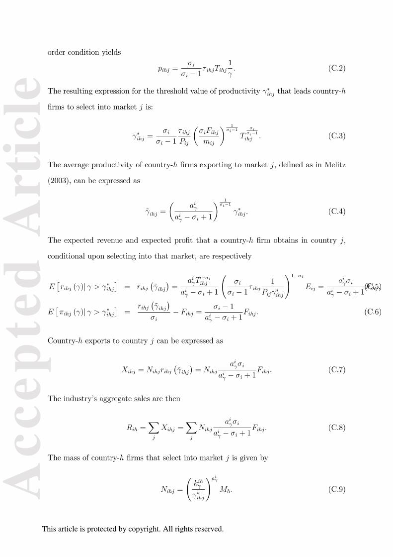
order condition yields
pihj =σi
σi − 1τ ihjTihj
1
γ. (C.2)
The resulting expression for the threshold value of productivity γ∗ihj that leads country-h
firms to select into market j is:
γ∗ihj =σi
σi − 1
τ ihjPij
(σiFihjmij
) 1σi−1
Tσiσi−1ihj . (C.3)
The average productivity of country-h firms exporting to market j, defined as in Melitz
(2003), can be expressed as
γihj =
(aiγ
aiγ − σi + 1
) 1σi−1
γ∗ihj. (C.4)
The expected revenue and expected profit that a country-h firm obtains in country j,
conditional upon selecting into that market, are respectively
E[rihj (γ)| γ > γ∗ihj
]= rihj
(γihj)
=aiγT
−σiihj
aiγ − σi + 1
(σi
σi − 1τ ihj
1
Pijγ∗ihj
)1−σi
Eij =aiγσi
aiγ − σi + 1Fihj,(C.5)
E[πihj (γ)| γ > γ∗ihj
]=
rihj(γihj)
σi− Fihj =
σi − 1
aiγ − σi + 1Fihj. (C.6)
Country-h exports to country j can be expressed as
Xihj = Nihjrihj(γihj)
= Nihj
aiγσi
aiγ − σi + 1Fihj. (C.7)
The industry’s aggregate sales are then
Rih =∑j
Xihj =∑j
Nihj
aiγσi
aiγ − σi + 1Fihj. (C.8)
The mass of country-h firms that select into market j is given by
Nihj =
(kihγγ∗ihj
)aiγ
Mh. (C.9)
This article is protected by copyright. All rights reserved.
Acc
epte
d A
rtic
le

Expected profits, aggregated across all destination markets, are
Πih =∑j
prob(γ > γ∗ihj
)E[πihj (γ)| γ > γ∗ihj
]=∑j
(kihγγ∗ihj
)aiγσi − 1
aiγ − σi + 1Fihj. (C.10)
Industry profits are therefore
MihΠih = Mih
∑j
(kihγγ∗ihj
)aiγσi − 1
aiγ − σi + 1Fihj =
σi − 1
aiγσi
∑j
Xihj. (C.11)
Industry employment can be easily shown to be
Lih = MihE [lihj (γ)] = Mih
∑j
(kihγγ∗ihj
)aiγ
E[lihj (γ)| γ > γ∗ihj
]= aiγMihΠih. (C.12)
and the price level Pij is given by
Pij =
aiγaiγ − σi + 1
∑h
Nihj
(σi
σi − 1
τ ihjTihjγ∗ihj
)1−σi 1
1−σi
. (C.13)
The expressions for industry level of growth rates are unchanged except for the price
index equation:
Pij =
[∑h
TihjXihj∑h TihjXihj
Nihj
(Tihj
)1−σi (γ∗ihj)σi−1
] 11−σi
. (C.14)
It is easy to show that
Pij =
[∑h
TihjXihj∑h TihjXihj
(Tihj
)1− σiσi−1
aiγ
]−1/aiγ
. (C.15)
We can use the system (C.15) to solve for the growth rates of the price levels Pij as a
function of the changes in tariffs Tihj. From equations (C.3), we can solve for γ∗ihj as a
function of Pij and Tihj,
γ∗ihj =
(Tihj
) σiσi−1
Pij. (C.16)
This article is protected by copyright. All rights reserved.
Acc
epte
d A
rtic
le

and thereafter generate predictions for the industry aggregates of interest.
This article is protected by copyright. All rights reserved.
Figures and Table
Figure 1: Increases in Trade Flows and Labor Productivity in Canada, 1988-1996
Notes: Figures show trade and labor productivity growth at the sectoral level (203 sectors) in
Canadian manufacturing, 1988 to 1996. Trade is measured as Canadian exports plus imports,labor
productivity is calculated as value added in production activities divided by total hours worked by
production workers(see Section 4.1 for details). All data are expressed in 1992 Canadian dollars using
4-digit industry price and value added deflators, and the 1992 US-Canadian exchange rate.
0
.00
5.0
1.0
15
.02
Den
sity
-100 0 100 200 300Labor Productivity Growth, %
0
.00
2.0
04
.00
6.0
08
Den
sity
0 500 1000 1500Trade Growth, %
Acc
epte
d A
rtic
le

Figure 2: Moment Deviations as a Function of aγ and σ (Trade and Productivity Growth, First Moment; Baseline Model)
Notes: See Section 4 for details.
0
10
20
30
40
0
10
20
30
40-2
-1
0
1
2
3
4
asigma
dev(d
X)
0
10
20
30
40
0
10
20
30
40
-0.29
-0.285
-0.28
-0.275
-0.27
-0.265
asigma
dev(d
VA
L d)
This article is protected by copyright. All rights reserved.
Acc
epte
d A
rtic
le
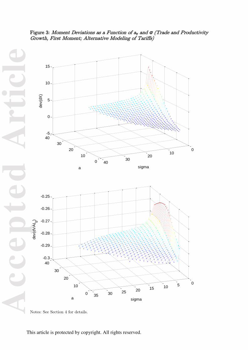
Figure 3: Moment Deviations as a Function of aγ and σ (Trade and Productivity Growth, First Moment; Alternative Modeling of Tariffs)
Notes: See Section 4 for details.
0
10
20
30
40
010
2030
40
-5
0
5
10
15
sigmaa
dev(d
X)
0
10
20
30
40
05101520253035
-0.3
-0.29
-0.28
-0.27
-0.26
-0.25
sigmaa
dev(d
VA
L d)
This article is protected by copyright. All rights reserved.
Acc
epte
d A
rtic
le

Table 1: Empirical Moments to Be Matched
Moment Mean(dX) Mean(dVAL) Cov(dX,dVAL) Var(dX) Var(dVAL) Data 1.1820 0.3041 0.1007 3.0130 0.1153
Notes: Table shows empirical moments to be matched by our theoretical models. 'dX' denotes trade
growth and 'dVAL' labor productivity growth (see Figure 1 and Section 4 for details).
Table 2: Results for Baseline Model (Matching Growth Rates 1988-1996)
Moments Mean(dX) Mean(dVAL) Cov(dX,dVAL) Var(dX) Var(dVAL) (1) Data 1.1820 0.3041 0.1007 3.0130 0.1153 (2) Model – Observed Parameter Values
0.3088 0.0139 0.0007 0.3373 0.0002
(3) Model – Optimised Parameter Values (First Step)
1.1408 0.0177 0.0039 3.0185 0.0002
(4) Model – Optimised Parameter Values (GMM)
1.0538 0.0174 0.0034 2.4004 0.0002
Parameters Optimised
(value, SE) Data (mean,
sd)
Σ 8.4942 3.4611 (121.9231) (0.8765) aγ 14.2482 5.0951 (1.1253)*** (2.6032) GMM objective (p-value) 91.7885 (0.00000)
Notes: dX denotes trade growth and dVAL' labor productivity growth (see Section 4 for details).
This article is protected by copyright. All rights reserved.
Acc
epte
d A
rtic
le

Table 3: Results for Baseline Model (Higher aγ and σ)
Moments Mean(dX) Mean(dVAL) Cov(dX,dVAL) Var(dX) Var(dVAL) (1) Data 1.1820 0.3041 0.1007 3.0130 0.1153 (2) Model – Observed
Parameter Values (σ x1.5) 0.7005 0.0153 0.0041 3.7584 0.0002
(3) Model – Observed
Parameter Values (σ x2) 1.3797 0.0169 0.0164 29.4970 0.0002
(3) Model – Observed
Parameter Values (σ x1.88, match mean trade growth)
1.1820 0.0165 0.0125 18.6332 0.0002
(4) Model – Observed Parameter Values (ar x1.5)
0.5674 0.0149 0.0022 1.9818 0.0002
(5) Model – Observed Parameter Values (ar x 2)
0.9529 0.0158 0.0077 9.6694 0.0002
(6) Model – Observed Parameter Values (ar x2.23, match mean trade growth)
1.1820 0.0163 0.0122 18.5781 0.0002
Notes: dX denotes trade growth and dVAL' labor productivity growth (see Section 4 for details).
This article is protected by copyright. All rights reserved.
Acc
epte
d A
rtic
le

Table 4: Results for Baseline Model (Drop Outliers)
Panel A: drop top and bottom 5%
Moments Mean(dX) Mean(dVAL) Cov(dX,dVAL) Var(dX) Var(dVAL)
(1) Data 0.9737 0.2858 0.0372 0.6675 0.0453
(2) Model – Observed Parameter Values
0.2893 0.0153 0.0005 0.1440 0.0002
(3) Model – Optimised Parameter Values (First Step)
0.7657 0.0171 0.0007 0.7436 0.0002
(4) Model – Optimised Parameter Values
0.8085 0.0183 0.0015 0.8770 0.0002
Parameters Optimised
(value, SE) Data (mean,
sd)
Σ 7.0894 3.5161
(72.9391) (0.9040)
aγ 12.5859 5.1936
(0.8968)*** (2.5479)
GMM objective (p-value) 107.378
(0.00000)
Panel B: drop top 5% only
(5) Data 0.8739 0.2495 0.0542 0.7049 0.0553
(6) Model – Observed Parameter Values
0.2679 0.0143 0.0006 0.1325 0.0002
(7) Model – Optimised Parameter Values (First Step)
0.7365 0.0162 0.0013 0.7526 0.0002
(8) Model – Optimised Parameter Values
0.7606 0.0172 0.0021 0.8324 0.0002
Parameters Optimised
(value, SE) Data (mean,
sd)
Σ 7.1215 3.5011
(80.0526) (0.8933)
aγ 12.6347 5.1776
(0.9331)*** (2.5549)
GMM objective (p-value) 112.996
(0.00000)
Notes: dX denotes trade growth and dVAL' labor productivity growth (see Section 4 for details).
This article is protected by copyright. All rights reserved.
Acc
epte
d A
rtic
le

Table 5: Results for Baseline Model (Prices at Factory Gate)
Moments Mean(dX) Mean(dVAL) Cov(dX,dVAL) Var(dX) Var(dVAL) (1) Data 1.1820 0.3041 0.1007 3.0130 0.1153 (2) Model – Observed Parameter Values
0.3857 0.0171 0.0005 0.4862 0.0002
(3) Model – Optimised Parameter Values (First Step)
1.1631 0.0198 0.0016 3.0156 0.0003
(4) Model – Optimised Parameter Values (GMM)
1.0653 0.0196 0.0014 2.3443 0.0003
Parameters Optimised
(value, SE) Data (mean, sd)
Σ 8.0972 3.4611 (127.1901) (0.8765) aγ 13.2980 5.0951 (1.3123)*** (2.6032) GMM objective (p-value)
90.6741
(0.00000)
Notes: dX denotes trade growth and dVAL' labor productivity growth (see Section 4 for details).
Table 6: Results for Baseline Model (Alternative Modeling Approach to Tariffs)
Moments Mean(dX) Mean(dVAL) Cov(dX,dVAL) Var(dX) Var(dVAL) (1) Data 1.1820 0.3041 0.1007 3.0130 0.1153 (2) Model – Observed Parameter Values
0.5154 0.0191 0.0029 1.3670 0.0003
(3) Model – Optimised Parameter Values (First Step)
1.1584 0.0330 0.0058 3.0195 0.0009
(4) Model – Optimised Parameter Values (GMM)
1.0705 0.0323 0.0050 2.3986 0.0009
Parameters Optimised
(value, SE) Data (mean, sd)
Σ 2.0101 3.4611 (1.5114) (0.8765) aγ 7.1208 5.0951 (5.3689) (2.6032) GMM objective (p-value)
85.6412
(0.00000)
Notes: dX denotes trade growth and dVAL' labor productivity growth (see Section 4 for details).
This article is protected by copyright. All rights reserved.
Acc
epte
d A
rtic
le
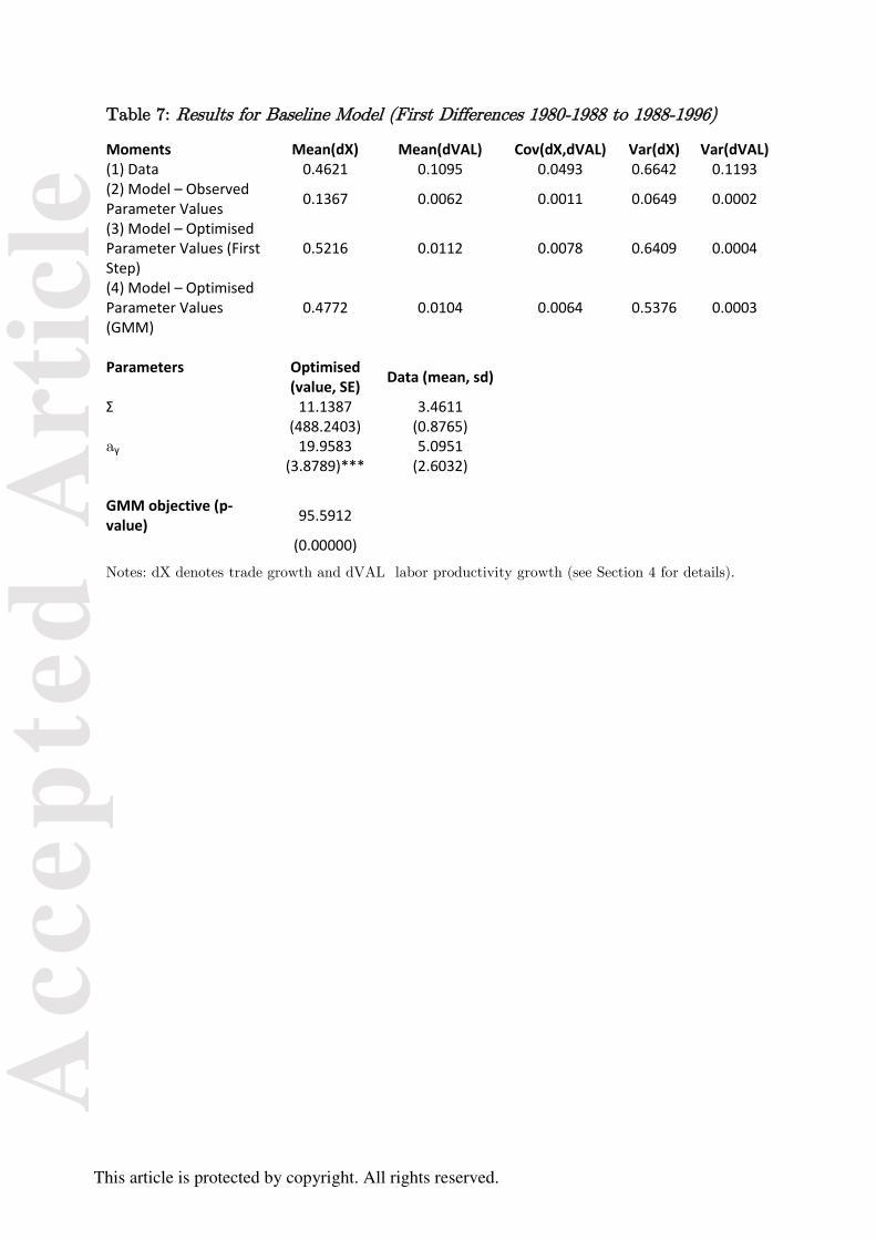
Table 7: Results for Baseline Model (First Differences 1980-1988 to 1988-1996)
Moments Mean(dX) Mean(dVAL) Cov(dX,dVAL) Var(dX) Var(dVAL) (1) Data 0.4621 0.1095 0.0493 0.6642 0.1193 (2) Model – Observed Parameter Values
0.1367 0.0062 0.0011 0.0649 0.0002
(3) Model – Optimised Parameter Values (First Step)
0.5216 0.0112 0.0078 0.6409 0.0004
(4) Model – Optimised Parameter Values (GMM)
0.4772 0.0104 0.0064 0.5376 0.0003
Parameters Optimised
(value, SE) Data (mean, sd)
Σ 11.1387 3.4611 (488.2403) (0.8765) aγ 19.9583 5.0951 (3.8789)*** (2.6032) GMM objective (p-value)
95.5912
(0.00000)
Notes: dX denotes trade growth and dVAL' labor productivity growth (see Section 4 for details).
This article is protected by copyright. All rights reserved.
Acc
epte
d A
rtic
le

Table 8: Results for Baseline Model (Diff-in-Diff Predicted Values)
Moments Mean(dX) Mean(dVAL) Cov(dX,dVAL) Var(dX) Var(dVAL) (1) Data 0.1457 0.0104 0.0087 0.0576 0.0044 (2) Model – Observed Parameter Values
0.1072 0.0032 0.0008 0.0292 0.0000
(3) Model – Optimised Parameter Values (First Step)
0.1487 0.0035 0.0013 0.0537 0.0000
(4) Model – Optimised Parameter Values (GMM)
0.1411 0.0017 0.0005 0.0483 0.0000
Parameters Optimised
(value, SE) Data (mean, sd)
Σ 8.2290 3.4611 (1.9631)*** (0.8765) aγ 7.2313 5.0951 (0.0983)*** (2.6032) GMM objective (p-value)
42.3101
(0.00000)
Notes: dX denotes trade growth and dVAL' labor productivity growth (see Section 4 for details).
This article is protected by copyright. All rights reserved.
Acc
epte
d A
rtic
le

Table 9: Results for Baseline Model (Changes in Non-Tariff Trade Costs)
Moments Mean(dX) Mean(dVAL) Cov(dX,dVAL) Var(dX) Var(dVAL) (1) Data 1.1820 0.3041 0.1007 3.0130 0.1153 (2) Model – Observed Parameter Values (c=1.1)
0.2055 0.0027 0.0073 1.5017 0.0004
(3) Model – Observed Parameter Values (c=0.9)
2.4642 0.0679 0.0481 65.7687 0.0029
(4) Model – Observed Parameter Values (c=0.98))
1.1820 0.0367 0.0225 15.0791 0.0011
(3) Model – Optimised Parameter Values (First Step)
1.1878 0.0187 0.0037 3.0124 0.0003
(4) Model – Optimised Parameter Values (GMM)
0.8924 0.2948 -0.0116 0.0582 0.0849
Parameters Optimised
(value, SE)
Σ 1.0100 (0.5206)* aγ 0.7209 (0.1059)*** c 0.4322 (0.0364)*** GMM objective (p-value) 9.7516 (0.0076)
Notes: dX denotes trade growth and dVAL' labor productivity growth (see Section 4 for details).
Table 10: Results for Baseline Model with Free Entry
Moments Mean(dX) Mean(dVAL) Cov(dX,dVAL) Var(dX) Var(dVAL) (1) Data 1.1820 0.3041 0.1007 3.0130 0.1153 (2) Model – Observed Parameter Values
0.3455 0.0076 0.0007 0.3877 0.0001
(3) Model – Optimised Parameter Values (First Step)
1.2533 0.0091 0.0116 3.2869 0.0002
(4) Model – Optimised Parameter Values (GMM)
1.1451 0.0090 0.0089 2.4802 0.0001
Parameters Optimised
(value, SE) Data (mean, sd)
σ 8.3205 3.4611 (90.6883) (0.8765) aγ 13.1861 5.0951 (0.8983) (2.6032) GMM objective (p-value) 83.2979
(0.0000)
Notes: dX denotes trade growth and dVAL' labor productivity growth (see Section 5 for details).
This article is protected by copyright. All rights reserved.
Acc
epte
d A
rtic
le

Table 11: Results for the ‘General Equilibrium’ Extension
Moments Mean(dX) Mean(dVAL) Cov(dX,dVAL) Var(dX) Var(dVAL) (1) Data 1.1820 0.3041 0.1007 3.0130 0.1153 (2) Model – Observed Parameter Values
0.3533 0.0088 0.0005 0.3863 0.0001
(3) Model – Optimised Parameter Values (First Step)
1.1310 0.0098 0.0147 3.2430 0.0001
(4) Model – Optimised Parameter Values (GMM)
0.9590 0.0119 0.0122 1.9985 0.0002
Parameters Optimised
(value, SE) Data (mean, sd)
Σ 7.1959 3.4611 (68.4995) (0.8765) aγ 11.5299 5.0951 (0.0796)*** (2.6032) GMM objective (p-value)
83.5599 (0.0000)
Notes: dX denotes trade growth and dVAL' labor productivity growth (see Section 5 for details).
Table 12: Results for the ‘Intermediate Inputs’ Extension
Moments Mean(dX) Mean(dVAL) Cov(dX,dVAL) Var(dX) Var(dVAL) (1) Data 1.1820 0.3041 0.1007 3.0130 0.1153 (2) Model – Observed Parameter Values
0.3541 0.0295 0.0100 0.5171 0.0020
(3) Model – Optimised Parameter Values (First Step)
1.2208 0.0466 0.0245 2.9930 0.0013
(4) Model – Optimised Parameter Values (GMM)
1.4581 0.1470 0.2139 3.7357 0.0393
Parameters Optimised
(value, SE) Data (mean, sd)
Σ 12.9013 3.4611 (0.0211)*** (0.8765) aγ 11.9700 5.0951 (0.0018)*** (2.6032) α 0.9871 0.7065 (0.0025)*** (0.0918) GMM objective (p-value)
44.8265 (0.0000)
Notes: dX denotes trade growth and dVAL' labor productivity growth (see Section 5 for details).
This article is protected by copyright. All rights reserved.
Acc
epte
d A
rtic
le

Table 13: Results for the Multiproduct-Firm Model
Moments Mean(dX) Mean(dVAL) Cov(dX,dVAL) Var(dX) Var(dVAL) (1) Data 1.1820 0.3041 0.1007 3.0130 0.1153 (2) Model – Observed Parameter Values
-- -- -- -- --
(3) Model –Optimised Parameter Values (First Step)
1.2392 0.2738 0.1552 3.0034 0.0976
(4) Model – Optimised Parameter Values (GMM)
1.2175 0.2855 0.1549 2.8239 0.1073
Parameters Optimised
(value, SE) Data (mean, sd)
Χ 1.1276 -- (0.0786)*** aγ 8.1552 -- (1.1506)*** aλ 4.9922 -- (0.5831)*** GMM objective (p-value)
3.3434 (0.1879)
Notes: dX denotes trade growth and dVAL' labor productivity growth (see Section 5 for details).
Table 14: Out-of-Sample Predictions
Model Parameters Moments d.o.f.
GMM objective in-sample (p-value)
GMM objective out-of-sample
Baseline 2 5 3 91.7885 (0.0000)
99.2693
Free entry 2 5 3 83.2979 (0.0000)
102.1245
General equilibrium 2 5 3 83.5599 (0.0000)
90.4165
Intermediates 3 5 2 44.2633 (0.0000)
106.2829
Multiproduct 3 5 2 3.3434
(0.1879) 42.7024
Notes: See Section 5 for details.
This article is protected by copyright. All rights reserved.
Acc
epte
d A
rtic
le

Online Appendix to: Tariffs, Trade andProductivity: A Quantitative Evaluation of
Heterogeneous Firm Models
Holger BreinlichUniversity of Essex, CEP and CEPR
Alejandro CuñatUniversity of Vienna and CES-ifo
September 29, 2014
1 Introduction
This appendix provides a detailed mathematical treatment of the models dis-cussed in the paper. For simplicity, each model is presented in a self-containedmanner.
2 Baseline model
2.1 Assumptions
2.1.1 Preferences
There are many countries. Each country admits a representative agent, withpreferences
U =∑i∈I
mi lnQi +A, (1)
where mi > 0. A denotes consumption of a homogeneous final good. Qi denotesconsumption of a Dixit-Stiglitz aggregate (manufacturing) final good i:1
Qi =
[∫γ∈Γi
qi(γ)ρidγ
] 1ρi
, (2)
where ρ ∈ (0, 1) and σ ≡ 1/ (1− ρ) denotes the elasticity of substitution betweenany two varieties. Choosing good A as the numéraire, utility maximization onthe upper level yields demand functions A = Y −
∑imi and Qi = mi/Pi, where
Y is total expenditure per consumer. In the manufacturing goods sector, utilitymaximization yields demand function qi(γ) = pi (γ)
−σPσ−1i mi.
1Wherever possible, we dispense with industry index i and with country indexes.
This article is protected by copyright. All rights reserved.
Acc
epte
d A
rtic
le
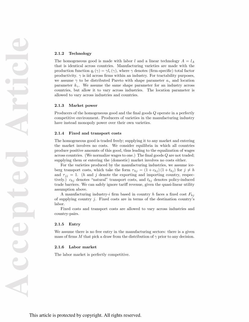
2.1.2 Technology
The homogeneous good is made with labor l and a linear technology A = lAthat is identical across countries. Manufacturing varieties are made with theproduction function qi (γ) = γli (γ), where γ denotes (firm-specific) total factorproductivity. γ is iid across firms within an industry. For tractability purposes,we assume γ to be distributed Pareto with shape parameter aγ and locationparameter kγ . We assume the same shape parameter for an industry acrosscountries, but allow it to vary across industries. The location parameter isallowed to vary across industries and countries.
2.1.3 Market power
Producers of the homogeneous good and the final goods Q operate in a perfectlycompetitive environment. Producers of varieties in the manufacturing industryhave instead monopoly power over their own varieties.
2.1.4 Fixed and transport costs
The homogeneous good is traded freely; supplying it to any market and enteringthe market involves no costs. We consider equilibria in which all countriesproduce positive amounts of this good, thus leading to the equalization of wagesacross countries. (We normalize wages to one.) The final goodsQ are not traded;supplying them or entering the (domestic) market involves no costs either.For the varieties produced by the manufacturing industries, we assume ice-
berg transport costs, which take the form τhj = (1 + chj) (1 + thj) for j 6= hand τ jj = 1. (h and j denote the exporting and importing country, respec-tively.) chj denotes “natural” transport costs, and thj denotes policy-inducedtrade barriers. We can safely ignore tariff revenue, given the quasi-linear utilityassumption above.A manufacturing industry-i firm based in country h faces a fixed cost Fhj
of supplying country j. Fixed costs are in terms of the destination country’slabor.Fixed costs and transport costs are allowed to vary across industries and
country-pairs.
2.1.5 Entry
We assume there is no free entry in the manufacturing sectors: there is a givenmass of firmsM that pick a draw from the distribution of γ prior to any decision.
2.1.6 Labor market
The labor market is perfectly competitive.
This article is protected by copyright. All rights reserved.
Acc
epte
d A
rtic
le

2.2 Firm-level and industry outcomes
The pricing decision over the variety produced by a country-h firm with pro-ductivity γ is the usual mark-up over marginal cost. Well-known manipulationof firm revenue and profit functions yields to the following expression for thethreshold value of productivity γ∗hj that leads country-h firms to select intomarket j:
γ∗hj =σ
σ − 1
τhjPj
(σFhjmj
) 1σ−1
. (3)
The average productivity of country-h firms exporting to market j, defined asin Melitz (2003), can be expressed as
γhj =
(aγ
aγ − σ + 1
) 1σ−1
γ∗hj . (4)
The expected revenue and expected profit that a country-h firm obtains incountry j, conditional upon selecting into that market, are respectively
E[rhj (γ)| γ > γ∗hj
]= rhj
(γhj)
=aγσ
aγ − σ + 1Fhj , (5)
E[πhj (γ)| γ > γ∗hj
]=
rhj(γhj)
σ− Fhj =
σ − 1
aγ − σ + 1Fhj . (6)
Country-h exports to country j can be expressed as
Xhj = Nhjrhj(γhj)
= Nhjaγσ
aγ − σ + 1Fhj . (7)
The industry’s aggregate sales are then
Rh =∑j
Xhj =∑j
Nhjaγσ
aγ − σ + 1Fhj . (8)
The mass of country-h firms that select into market j is given by
Nhj =
(khγ∗hj
)aγMh. (9)
Expected profits, aggregated across all destination markets, are
Πh =∑j
prob(γ > γ∗hj
)E[πhj (γ)| γ > γ∗hj
]=∑j
(khγ∗hj
)aγσ − 1
aγ − σ + 1Fhj .
(10)Industry profits are therefore
MhΠh = Mh
∑j
(khγ∗hj
)aγσ − 1
aγ − σ + 1Fhj =
σ − 1
aγσ
∑j
Xhj . (11)
This article is protected by copyright. All rights reserved.
Acc
epte
d A
rtic
le

Industry employment can be easily shown to be
Lh = MhE [lhj (γ)] = Mh
∑j
(khγ∗hj
)aγE[lhj (γ)| γ > γ∗hj
]= aγMhΠh. (12)
The price level Pj is given by
Pj =
aγaγ − σ + 1
∑h
Nhj
(σ
σ − 1
τhjγ∗hj
)1−σ 1
1−σ
. (13)
Melitz (2003) defines industry productivity as
γh =
∑j
Nhj∑j Nhj
(γhj)σ−1
1σ−1
. (14)
2.3 Growth rates
The growth rates of the industry’s aggregates can be expressed as functionsof parameter values, changes in τhj , changes in thresholds γ∗hj , and the lev-els of bilateral trade Xhj . Define x ≡ x′/x as a gross growth rate, where xand x′ denote, respectively, the values of a variable before and after the tradeliberalization:
Xhj = Nhj =(γ∗hj)−aγ
, (15)
Rh = Πh = Lh =∑j
Xhj∑j Xhj
Xhj , (16)
Pj =
[∑h
Xhj∑hXhj
Nhj (τhj)1−σ (
γ∗hj)σ−1
] 11−σ
. (17)
As a measurable proxy for productivity growth, we will consider the growth rateof deflated value added per worker,
Rh
Lh
p (γh)
p(γ′h) =
Rh
Lh
γ′hγh
=γ′hγh, (18)
where we use the price charged by the firm with average productivity p (γh) asa deflator. (See Section 3 and Appendix A in the paper for a detailed discussionof the appropriate choice of deflator.) The growth rate γ′h/γh can be written as
γ′hγh
=
∑
j
(N ′hjNhj
Nhj∑j′ Nhj′
)−1∑j
N ′hjNhj
(γ′hjγhj
)σ−1Nhj
(γhj)σ−1∑
j′ Nhj′(γhj′
)σ−1
1σ−1
.
(19)
This article is protected by copyright. All rights reserved.
Acc
epte
d A
rtic
le

We do not have data for Nhj , but under the assumption that entry costs areproportional to some observable destination-specific factor that is exogenous tothe model (such as mj , GDP, population, area,...):
Nhj∑j′ Nhj′
=Xhj/
(aγσ
aγ−σ+1
)Fhj∑
j′ Xhj′/(
aγσaγ−σ+1
)Fhj′
=Xhj/mj∑j′ Xhj′/mj′
. (20)
From (4) and (9),
γhj =
(aγ
aγ − σ + 1
) 1σ−1
γ∗hj =
(aγ
aγ − σ + 1
) 1σ−1
kh (Mh)1aγ N
− 1aγ
hj . (21)
We can approximate
Nhj(γhj)σ−1∑
j′ Nhj′(γhj′
)σ−1 =(Xhj/mj)
1−σ+aγaγ∑
j′ (Xhj′/mj′)1−σ+aγaγ
. (22)
2.4 Predictions
It is easy to show that
Pj =
[∑h
Xhj∑hXhj
τ−aγhj
]−1/aγ
. (23)
We can use the system (23) to solve for the growth rates of the price levels Pjas a function of the changes in transport costs τhj . From equations (3), we cansolve for γ∗hj as a function of Pj and τhj ,
γ∗hj = τhj/Pj , (24)
and thereafter generate predictions for the industry aggregates of interest.
3 Free entry
3.1 Assumptions
3.1.1 Preferences
There are many countries. Each country admits a representative agent, withpreferences
U =∑i∈I
mi lnQi +A, (25)
This article is protected by copyright. All rights reserved.
Acc
epte
d A
rtic
le

where mi > 0. A denotes consumption of a homogeneous final good. Qi denotesconsumption of a Dixit-Stiglitz aggregate (manufacturing) final good i:2
Qi =
[∫γ∈Γi
qi(γ)ρidγ
] 1ρi
, (26)
where ρ ∈ (0, 1) and σ ≡ 1/ (1− ρ) denotes the elasticity of substitution betweenany two varieties. Choosing good A as the numéraire, utility maximization onthe upper level yields demand functions A = Y −
∑imi and Qi = mi/Pi, where
Y is total expenditure per consumer. In the manufacturing goods sector, utilitymaximization yields demand function qi(γ) = pi (γ)
−σPσ−1i mi.
3.1.2 Technology
The homogeneous good is made with labor l and a linear technology A = lAthat is identical across countries. Manufacturing varieties are made with theproduction function qi (γ) = γli (γ), where γ denotes (firm-specific) total factorproductivity. γ is iid across firms within an industry. For tractability purposes,we assume γ to be distributed Pareto with shape parameter aγ and locationparameter kγ . We assume the same shape parameter for an industry acrosscountries, but allow it to vary across industries. The location parameter isallowed to vary across industries and countries.
3.1.3 Market power
Producers of the homogeneous good and the final goods Q operate in a perfectlycompetitive environment. Producers of varieties in the manufacturing industryhave instead monopoly power over their own varieties.
3.1.4 Fixed and transport costs
The homogeneous good is traded freely; supplying it to any market and enteringthe market involves no costs. We consider equilibria in which all countriesproduce positive amounts of this good, thus leading to the equalization of wagesacross countries. (We normalize wages to one.) The final goodsQ are not traded;supplying them or entering the (domestic) market involves no costs either.For the varieties produced by the manufacturing industries, we assume ice-
berg transport costs, which take the form τhj = (1 + chj) (1 + thj) for j 6= hand τ jj = 1. (h and j denote the exporting and importing country, respec-tively.) chj denotes “natural” transport costs, and thj denotes policy-inducedtrade barriers. We can safely ignore tariff revenue, given the quasi-linear utilityassumption above.A manufacturing industry-i firm based in country h faces a fixed cost Fhj
of supplying country j. Fixed costs are in terms of the destination country’slabor.
2Wherever possible, we dispense with industry index i and with country indexes.
This article is protected by copyright. All rights reserved.
Acc
epte
d A
rtic
le

Fixed costs and transport costs are allowed to vary across industries andcountry-pairs.
3.1.5 Entry
We assume free entry: the mass of firms Mji active in an industry is the resultof firms comparing expected profits with the fixed cost Fji (in terms of countryj’s labor) that they have to pay in order to pick a draw from the distributionof γ. Fji is allowed to vary across industries and countries.
3.1.6 Labor market
The labor market is perfectly competitive.
3.2 Firm-level and industry outcomes
The pricing decision over the variety produced by a country-h firm with pro-ductivity γ is the usual mark-up over marginal cost. Well-known manipulationof firm revenue and profit functions yields to the following expression for thethreshold value of productivity γ∗hj that leads country-h firms to select intomarket j:
γ∗hj =σ
σ − 1
τhjPj
(σFhjmj
) 1σ−1
. (27)
The average productivity of country-h firms exporting to market j, defined asin Melitz (2003), can be expressed as
γhj =
(aγ
aγ − σ + 1
) 1σ−1
γ∗hj . (28)
The expected revenue and expected profit that a country-h firm obtains incountry j, conditional upon selecting into that market, are respectively
E[rhj (γ)| γ > γ∗hj
]= rhj
(γhj)
=aγσ
aγ − σ + 1Fhj , (29)
E[πhj (γ)| γ > γ∗hj
]=
rhj(γhj)
σ− Fhj =
σ − 1
aγ − σ + 1Fhj . (30)
Country-h exports to country j can be expressed as
Xhj = Nhjrhj(γhj)
= Nhjaγσ
aγ − σ + 1Fhj . (31)
The industry’s aggregate sales are then
Rh =∑j
Xhj =∑j
Nhjaγσ
aγ − σ + 1Fhj . (32)
This article is protected by copyright. All rights reserved.
Acc
epte
d A
rtic
le

The mass of country-h firms that select into market j is given by
Nhj =
(khγ∗hj
)aγMh. (33)
The free-entry condition sets expected profits equal to the fixed cost Fh:∑j
prob(γ > γ∗hj
)E[πhj (γ)| γ > γ∗hj
]= Fh. (34)
Industry employment can be easily shown to be
Lh = MhE [lhj (γ)] = Mh
∑j
(khγ∗hj
)aγE[lhj (γ)| γ > γ∗hj
]=σ − 1
σRh. (35)
The price level Pj is given by
Pj =
aγaγ − σ + 1
∑h
Nhj
(σ
σ − 1
τhjγ∗hj
)1−σ 1
1−σ
. (36)
Melitz (2003) defines industry productivity as
γh =
∑j
Nhj∑j Nhj
(γhj)σ−1
1σ−1
. (37)
3.3 Growth rates
The growth rates of the industry’s aggregates can be expressed as functionsof parameter values, changes in τhj , changes in thresholds γ∗hj , and the lev-els of bilateral trade Xhj . Define x ≡ x′/x as a gross growth rate, where xand x′ denote, respectively, the values of a variable before and after the tradeliberalization:
Xhj = Nhj =(γ∗hj)−aγ
Mh, (38)
Rh = Lh =∑j
Xhj∑j Xhj
Xhj , (39)
Pj =
[∑h
Xhj∑hXhj
Nhj (τhj)1−σ (
γ∗hj)σ−1
] 11−σ
. (40)
As a measurable proxy for productivity growth, we will consider the growth rateof deflated value added per worker,
Rh
Lh
p (γh)
p(γ′h) =
Rh
Lh
γ′hγh
=γ′hγh, (41)
This article is protected by copyright. All rights reserved.
Acc
epte
d A
rtic
le

where we use the price charged by the firm with average productivity p (γh) asa deflator. (See Section 3 and Appendix A in the paper for a detailed discussionof the appropriate choice of deflator.) The growth rate γ′h/γh can be written as
γ′hγh
=
∑
j
(N ′hjNhj
Nhj∑j′ Nhj′
)−1∑j
N ′hjNhj
(γ′hjγhj
)σ−1Nhj
(γhj)σ−1∑
j′ Nhj′(γhj′
)σ−1
1σ−1
.
(42)We do not have data for Nhj , but under the assumption that entry costs areproportional to some observable destination-specific factor that is exogenous tothe model (such as mj , GDP, population, area,...):
Nhj∑j Nhj
=Xhj/
(aγσ
aγ−σ+1
)Fhj∑
j Xhj/(
aγσaγ−σ+1
)Fhj
=Xhj/mj∑j Xhj/mj
. (43)
From (28) and (33),
γhj =
(aγ
aγ − σ + 1
) 1σ−1
γ∗hj =
(aγ
aγ − σ + 1
) 1σ−1
kh (Mh)1aγ N
− 1aγ
hj . (44)
We can approximate
Nhj(γhj)σ−1∑
j′ Nhj′(γhj′
)σ−1 =(Xhj/mj)
1−σ+aγaγ∑
j′ (Xhj′/mj′)1−σ+aγaγ
. (45)
3.4 Predictions
Manipulating the growth rates of the free-entry condition and the price level,
1 =∑j
Xhj∑nXhn
τ−aγhj P
aγj , (46)
P−aγj =
∑h
Xhj∑hXhj
Mhτ−aγhj . (47)
Once we have the values of Pj and Mj , we can generate the model’s predictionsfor all variables of interest.
This article is protected by copyright. All rights reserved.
Acc
epte
d A
rtic
le

4 Intermediate inputs
4.1 Assumptions
4.1.1 Preferences
There are many countries. Each country admits a representative agent, withpreferences
U =∑i∈I
mi lnQci +A, (48)
wheremi > 0. A denotes consumption of a homogeneous final good. Qci denotesconsumption of a Dixit-Stiglitz aggregate (manufacturing) final good Qi:3
Qi =
[∫γ∈Γi
qi(γ)ρidγ
] 1ρi
, (49)
where ρ ∈ (0, 1) and σ ≡ 1/ (1− ρ) denotes the elasticity of substitution betweenany two varieties. Choosing good A as the numéraire, utility maximization onthe upper level yields demand functions A = Y −
∑imi and Qi = mi/Pi, where
Y is total expenditure per consumer. In the manufacturing goods sector, utilitymaximization yields demand function qi(γ) = pi (γ)
−σPσ−1i mi.
4.1.2 Technology
The homogeneous good is made with labor l and a linear technology A = lAthat is identical across countries. Manufacturing varieties are made with thefollowing production function:
qi (γ) = γ
[Qinputi (γ)
α
]α [l (γ)
1− α
]1−α. (50)
Qinputi denotes the amount of the aggregate manufacturing good used as anintermediate input; α ∈ [0, 1); γ denotes (firm-specific) total factor productivityand is iid across firms within an industry. For tractability purposes, we assumeγ to be distributed Pareto with shape parameter aγ and location parameterkγ . We assume the same shape parameter for an industry across countries, butallow it to vary across industries. The location parameter is allowed to varyacross industries and countries.
4.1.3 Market power
Producers of the homogeneous good and the final goods Q operate in a perfectlycompetitive environment. Producers of varieties in the manufacturing industryhave instead monopoly power over their own varieties.
3Wherever possible, we dispense with industry index i and with country indexes.
This article is protected by copyright. All rights reserved.
Acc
epte
d A
rtic
le
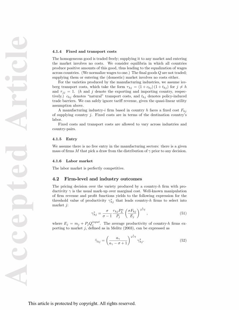
4.1.4 Fixed and transport costs
The homogeneous good is traded freely; supplying it to any market and enteringthe market involves no costs. We consider equilibria in which all countriesproduce positive amounts of this good, thus leading to the equalization of wagesacross countries. (We normalize wages to one.) The final goodsQ are not traded;supplying them or entering the (domestic) market involves no costs either.For the varieties produced by the manufacturing industries, we assume ice-
berg transport costs, which take the form τhj = (1 + chj) (1 + thj) for j 6= hand τ jj = 1. (h and j denote the exporting and importing country, respec-tively.) chj denotes “natural” transport costs, and thj denotes policy-inducedtrade barriers. We can safely ignore tariff revenue, given the quasi-linear utilityassumption above.A manufacturing industry-i firm based in country h faces a fixed cost Fhj
of supplying country j. Fixed costs are in terms of the destination country’slabor.Fixed costs and transport costs are allowed to vary across industries and
country-pairs.
4.1.5 Entry
We assume there is no free entry in the manufacturing sectors: there is a givenmass of firmsM that pick a draw from the distribution of γ prior to any decision.
4.1.6 Labor market
The labor market is perfectly competitive.
4.2 Firm-level and industry outcomes
The pricing decision over the variety produced by a country-h firm with pro-ductivity γ is the usual mark-up over marginal cost. Well-known manipulationof firm revenue and profit functions yields to the following expression for thethreshold value of productivity γ∗hj that leads country-h firms to select intomarket j:
γ∗hj =σ
σ − 1
τhjPαh
Pj
(σFhjEj
) 1σ−1
, (51)
where Ej = mj + PjQinputj . The average productivity of country-h firms ex-
porting to market j, defined as in Melitz (2003), can be expressed as
γhj =
(aγ
aγ − σ + 1
) 1σ−1
γ∗hj . (52)
This article is protected by copyright. All rights reserved.
Acc
epte
d A
rtic
le

The expected revenue and expected profit that a country-h firm obtains incountry j, conditional upon selecting into that market, are respectively
E[rhj (γ)| γ > γ∗hj
]= rhj
(γhj)
=aγσ
aγ − σ + 1Fhj , (53)
E[πhj (γ)| γ > γ∗hj
]=
rhj(γhj)
σ− Fhj =
σ − 1
aγ − σ + 1Fhj . (54)
Country-h exports to country j can be expressed as
Xhj = Nhjrhj(γhj)
= Nhjaγσ
aγ − σ + 1Fhj . (55)
The industry’s aggregate sales are then
Rh =∑j
Xhj =∑j
Nhjaγσ
aγ − σ + 1Fhj . (56)
The mass of country-h firms that select into market j is given by
Nhj =
(khγ∗hj
)aγMh. (57)
Expected profits, aggregated across all destination markets, are
Πh =∑j
prob(γ > γ∗hj
)E[πhj (γ)| γ > γ∗hj
]=∑j
(khγ∗hj
)aγσ − 1
aγ − σ + 1Fhj .
(58)Industry profits are therefore
MhΠh = Mh
∑j
(khγ∗hj
)aγσ − 1
aγ − σ + 1Fhj =
σ − 1
aγσ
∑j
Xhj . (59)
Industry employment can be easily shown to be
Lh = MhE [lhj (γ)] = Mh
∑j
(khγ∗hj
)aγE[lhj (γ)| γ > γ∗hj
]= (1− α) aγMhΠh.
(60)Similarly, industry demand for intermediate input Qinput can be shown to be
Qinputh = MhE[Qinputh (γ)
]=αaγPh
MhΠh.
The price level Pj is given by
Pj =
aγaγ − σ + 1
∑h
Nhj
(σ
σ − 1
τhjPαh
γ∗hj
)1−σ 1
1−σ
. (61)
This article is protected by copyright. All rights reserved.
Acc
epte
d A
rtic
le

Melitz (2003) defines industry productivity as
γh =
∑j
Nhj∑j Nhj
(γhj)σ−1
1σ−1
. (62)
4.3 Growth rates
The growth rates of the industry’s aggregates can be expressed as functionsof parameter values, changes in τhj , changes in thresholds γ∗hj , and the lev-els of bilateral trade Xhj . Define x ≡ x′/x as a gross growth rate, where xand x′ denote, respectively, the values of a variable before and after the tradeliberalization:
Xhj = Nhj =(γ∗hj)−aγ
, (63)
Rh = Πh = Lh =∑j
Xhj∑j Xhj
Xhj , (64)
Pj =
[∑h
Xhj∑hXhj
Nhj (τhj)1−σ
(Pαh
)1−σ (γ∗hj)σ−1
] 11−σ
. (65)
Our measurable proxy for industry productivity, deflated value added per worker,is now defined as4
V Ahp (γh)Lh
=Rh − PhQinputh
p (γh)Lh. (66)
Taking growth rates,
RjRj − PjQinputj Πj
V A
1(Pj
)αLj
γ′
γ=(Pj
)−α γ′γ
(67)
The growth rate γ′h/γh can be written as
γ′hγh
=
∑
j
(N ′hjNhj
Nhj∑j′ Nhj′
)−1∑j
N ′hjNhj
(γ′hjγhj
)σ−1Nhj
(γhj)σ−1∑
j′ Nhj′(γhj′
)σ−1
1σ−1
.
(68)We do not have data for Nhj , but under the assumption that entry costs areproportional to some observable destination-specific factor that is exogenous tothe model (such as mj , GDP, population, area,...):
Nhj∑j Nhj
=Xhj/
(aγσ
aγ−σ+1
)Fhj∑
j Xhj/(
aγσaγ−σ+1
)Fhj
=Xhj/mj∑j Xhj/mj
. (69)
4See Section 3 and Appendix A in the paper for a detailed discussion of the appropriatechoice of deflator.
This article is protected by copyright. All rights reserved.
Acc
epte
d A
rtic
le

From (52) and (57),
γhj =
(aγ
aγ − σ + 1
) 1σ−1
γ∗hj =
(aγ
aγ − σ + 1
) 1σ−1
kh (Mh)1aγ N
− 1aγ
hj . (70)
We can approximate
Nhj(γhj)σ−1∑
j′ Nhj′(γhj′
)σ−1 =(Xhj/mj)
1−σ+aγaγ∑
j′ (Xhj′/mj′)1−σ+aγaγ
. (71)
4.4 Predictions
The price equation in changes can be rewritten as
Paγσ−1j =
(Ej
)σ−aγ−1(1−σ)2
[∑h
Xhj∑mXmj
τ−aγhj
1
Pαaγh
] 11−σ
, (72)
where
Ej =1
Ej
[mj + PjQ
inputj P
−aγαj
(∑h
Xjh∑hXjh
τ−aγjh P
aγh E
aγσ−1h
)]. (73)
This yields a system of non-linear equations in Pj and Ej . Once we have P. andE, we can solve for the remaining growth rates in the following order: γ∗jj , γ
∗hj ,
Nhj , Xhj , Πj , and thus Rj , Lj and Qinputj .
5 General equilibrium
5.1 Assumptions
5.1.1 Preferences
There are many countries. Each country admits a representative agent, withpreferences
U =∏i
Qµii , (74)
where µi > 0,∑i µi = 1. Qi denotes consumption of a Dixit-Stiglitz aggregate
(manufacturing) final good i:5
Qi =
[∫γ∈Γi
qi(γ)ρidγ
] 1ρi
, (75)
where ρ ∈ (0, 1) and σ ≡ 1/ (1− ρ) denotes the elasticity of substitution betweenany two varieties.
5Wherever possible, we dispense with industry index i and with country indexes.
This article is protected by copyright. All rights reserved.
Acc
epte
d A
rtic
le

5.1.2 Technology
Manufacturing varieties are made with the production function qi (γ) = γli (γ),where γ denotes (firm-specific) total factor productivity. γ is iid across firmswithin an industry. For tractability purposes, we assume γ to be distributedPareto with shape parameter aγ and location parameter kγ . We assume thesame shape parameter for an industry across countries, but allow it to varyacross industries. The location parameter is allowed to vary across industriesand countries.
5.1.3 Market power
Producers of the final goods Q operate in a perfectly competitive environment.Producers of varieties in the manufacturing industry have instead monopolypower over their own varieties.
5.1.4 Fixed and transport costs
The final goods Q are not traded; supplying them or entering the (domestic)market involves no costs either.For the varieties produced by the manufacturing industries, we assume ice-
berg transport costs, which take the form τhj = (1 + chj) (1 + thj) for j 6= hand τ jj = 1. (h and j denote the exporting and importing country, respec-tively.) chj denotes “natural” transport costs, and thj denotes policy-inducedtrade barriers. We ignore tariff revenue for comparability purposes with the restof the models.6
A manufacturing industry-i firm based in country h faces a fixed cost Fhjof supplying country j. Fixed costs are in terms of the destination country’slabor.Fixed costs and transport costs are allowed to vary across industries and
country-pairs.
5.1.5 Entry
We assume free entry: the mass of firms Mji active in an industry is the resultof firms comparing expected profits with the fixed cost Fji (in terms of countryj’s labor) that they have to pay in order to pick a draw from the distributionof γ. Fji is allowed to vary across industries and countries.
5.1.6 Labor market
The labor market is perfectly competitive. In each country j, Lj units of laborare supplied inelastically.
6Modeling tariff revenue in terms of lump-sum transfers to the levying country’s consumersdoes not change the model’s quantitative implications significantly. Results available from theauthors upon request.
This article is protected by copyright. All rights reserved.
Acc
epte
d A
rtic
le

5.2 Firm-level and industry outcomes
The pricing decision over the variety produced by a country-h firm with pro-ductivity γ is the usual mark-up over marginal cost. Well-known manipulationof firm revenue and profit functions yields to the following expression for thethreshold value of productivity γ∗hj that leads country-h firms to select intomarket j:
γ∗hj =σ
σ − 1
τhjwhPj
(σwjFhjµjwjLj
) 1σ−1
. (76)
The average productivity of country-h firms exporting to market j, defined asin Melitz (2003), can be expressed as
γhj =
(aγ
aγ − σ + 1
) 1σ−1
γ∗hj . (77)
The expected revenue and expected profit that a country-h firm obtains incountry j, conditional upon selecting into that market, are respectively
E[rhj (γ)| γ > γ∗hj
]= rhj
(γhj)
=aγσ
aγ − σ + 1wjFhj , (78)
E[πhj (γ)| γ > γ∗hj
]=
rhj(γhj)
σ− Fhj =
σ − 1
aγ − σ + 1wjFhj . (79)
Country-h exports to country j can be expressed as
Xhj = Nhjrhj(γhj)
= Nhjaγσ
aγ − σ + 1wjFhj . (80)
The industry’s aggregate sales are then
Rh =∑j
Xhj =∑j
Nhjaγσ
aγ − σ + 1wjFhj . (81)
The mass of country-h firms that select into market j is given by
Nhj =
(khγ∗hj
)aγMh. (82)
The free-entry condition sets expected profits equal to the fixed cost Fh:∑j
prob(γ > γ∗hj
)E[πhj (γ)| γ > γ∗hj
]= whFh. (83)
Industry employment can be easily shown to be
Lh = MhE [lhj (γ)] = Mh
∑j
(khγ∗hj
)aγE[lhj (γ)| γ > γ∗hj
]= aγMhFh =
σ − 1
σ
Rhwh
.
(84)
This article is protected by copyright. All rights reserved.
Acc
epte
d A
rtic
le

The labor market clearing condition sets Lh equal to the demand for labor(inclusive of fixed costs):
Lj =∑i
Mij
(1 + aiγ
)F ij +
∑i
[aiγ − σi + 1
wjaiγσi
(∑h
Xihj
)]. (85)
Thus,
wjLj =∑i
[(1 + aiγ
) (σi − 1
)aiγσ
i
(∑h
Xijh
)]+∑i
[aiγ − σi + 1
aiγσi
(∑h
Xihj
)].
(86)The price level Pj is given by
Pj =
aγaγ − σ + 1
∑h
Nhj
(σ
σ − 1
τhjwhγ∗hj
)1−σ 1
1−σ
. (87)
Melitz (2003) defines industry productivity as
γh =
∑j
Nhj∑j Nhj
(γhj)σ−1
1σ−1
. (88)
5.3 Growth rates
The growth rates of the industry’s aggregates can be expressed as functionsof parameter values, changes in τhj , changes in thresholds γ∗hj , and the lev-els of bilateral trade Xhj . Define x ≡ x′/x as a gross growth rate, where xand x′ denote, respectively, the values of a variable before and after the tradeliberalization:
Xhj = wjNhj = wj(γ∗hj)−aγ
Mh, (89)
Rh =∑j
Xhj∑j Xhj
Xhj , (90)
Lh = Rh/wh, (91)
Pj =
[∑h
Xhj∑hXhj
Nhj (τhj)1−σ
(wh)1−σ (
γ∗hj)σ−1
] 11−σ
. (92)
As a measurable proxy for productivity growth, we will consider the growth rateof deflated value added per worker,
Rh
Lh
p (γh)
p(γ′h) =
Rh
whLh
γ′hγh
=γ′hγh, (93)
This article is protected by copyright. All rights reserved.
Acc
epte
d A
rtic
le

where we use the price charged by the firm with average productivity p (γh) asa deflator. (See Section 3 and Appendix A in the paper for a detailed discussionof the appropriate choice of deflator.) The growth rate γ′h/γh can be written as
γ′hγh
=
∑
j
(N ′hjNhj
Nhj∑j′ Nhj′
)−1∑j
N ′hjNhj
(γ′hjγhj
)σ−1Nhj
(γhj)σ−1∑
j′ Nhj′(γhj′
)σ−1
1σ−1
.
(94)We do not have data for Nhj , but under the assumption that entry costs areproportional to some observable destination-specific factor that is exogenous tothe model:
Nhj∑j′ Nhj′
=Xhj/
(aγσ
aγ−σ+1
)wjFhj∑
j′ Xhj′/(
aγσaγ−σ+1
)wj′Fhj′
=Xhj/wjLj∑j′ Xhj′/wj′Lj′
(95)
where Lj is our choice of factor exogeneous to the model. Multiplying by wjyields GDP in the model which we use as the empirical proxy for wjLj . From(77) and (82),
γhj =
(aγ
aγ − σ + 1
) 1σ−1
γ∗hj =
(aγ
aγ − σ + 1
) 1σ−1
kh (Mh)1aγ N
− 1aγ
hj . (96)
We can approximate
Nhj(γhj)σ−1∑
j′ Nhj′(γhj′
)σ−1 =(Xhj/wjLj)
1−σ+aγaγ∑
j′ (Xhj′/wj′Lj′)1−σ+aγaγ
(97)
5.4 Predictions
The growth rates of the free entry condition, the price level and the labormarket clearing condition solve for the variables we need to generate predictions(Mj , wj , Pj). ∑
j
Xhj∑nXhn
(γ∗hj)−aγ
wj = wh, (98)
Pj =
[∑h
Xhj∑mXmj
Nhj (τhj)1−σ
(wh)1−σ (
γ∗hj)σ−1
] 11−σ
, (99)
wjLj =A
A+BA+
B
A+BB, (100)
This article is protected by copyright. All rights reserved.
Acc
epte
d A
rtic
le
where
γ∗hj =τhjwhwj
γ∗jj , (101)
γ∗jj =wj
Pj, (102)
Nhj =(γ∗hj)−a
Mh, (103)
and
A =∑i
[(1 + aiγ
) (σi − 1
)aiγσ
i
(∑h
Xijh
)], (104)
B =∑i
[aiγ − σi + 1
aiγσi
(∑h
Xihj
)], (105)
A =1
A
∑i
(1 + aiγ) (σi − 1
)aiγσ
i
(∑h
Xijh
) (∑h
Xijh
) , (106)
B =1
B
∑h
aiγ − σi + 1
aiγσi
(∑h
Xihj
) (∑h
Xihj
) . (107)
5.5 Other general equilibrium effects
If we consider trade deficits, then expenditure on industry i becomes
Eji = µji (wjLj + TDj) . (108)
Productivity thresholds are now
γ∗hji =σ
σ − 1
τhjiwhPji
(σwjFhjiEji
) 1σ−1
, (109)
with growth rates
γ∗hji =τhjiwhwj
γ∗jji, (110)
γ∗jj =wj
Pj
(wj
Eji
) 1σ−1
. (111)
The growth rate of Ej is
Eji =wjLj
(wjLj + TDj)wj +
TDj
(wjLj + TDj)
TD′jTDj
. (112)
This article is protected by copyright. All rights reserved.
Acc
epte
d A
rtic
le
6 Multi-product firms7
6.1 Assumptions
Uj =∑i∈I
µji lnQji +Aj , (113)
where i denotes industries and j denotes countries. Let us call Qji “final goods”and Aj the “numéraire” good. Utility maximization yields demand functionsA = Y −
∑imi and Qi = mi/Pi, where Y is total expenditure per consumer.
The homogeneous good is made with labor l and a linear technology A = lAthat is identical across countries. It is traded freely: supplying it to any marketand entering the market involves no costs. We consider equilibria in which allcountries produce positive amounts of this good, thus leading to the equalizationof wages across countries. (We normalize wages to one.)Final goods are made with a continuum of “products”, which are imperfect
substitutes in demand:
Qji =
(∫ 1
0
Cνjikdk
) 1ν
, (114)
where ν ∈ (0, 1) and k denotes product.
Pji =
(∫ 1
0
P 1−κjik dk
) 11−κ
. (115)
Within each product-industry, firms supply horizontally differentiated “vari-eties”of the product:8
Cjik =
[∑h
∫ω∈Ωhjik
[λhjik (ω) chjik (ω)]ρdω
] 1ρ
, (116)
where ρ ∈ (0, 1); h denotes the product’s country of origin; and χ ≡ 1/ (1− ρ) >κ ≡ 1/ (1− ν); λhjik (ω) captures “product attributes”, to be discussed below.The ideal price index associated to Cjik is
Pjik =
[∑h
∫ω∈Ωhjik
[phjik (ω)
λhjik (ω)
]1−χdω
] 11−χ
. (117)
There is a given mass of firms in each country/industry. (That is, we are inthe no-free-entry case.) After observing their γ and λ, firms decide whether theywant to pay fixed costs to select into different markets/products: (i) Firms basedin country h face a fixed cost Fhji of supplying country j. (ii) Besides Fhji, inorder to supply one variety of a product in country j, country-h firms must pay
7This section draws upon Bernard, A., S.J. redding and P.K. Schott (2011): “Multi-productFirms and Trade Liberalization,”Quarterly Journal of Economics, 126(3), pp.1271-1318.
8Firms are assumed to operate only within one industry.
This article is protected by copyright. All rights reserved.
Acc
epte
d A
rtic
le

fixed cost fhji. (Firms cannot supply more than one variety of each product byassumption.) (iii) Fixed costs are in terms of the destination country’s labor.There is a firm-specific constant marginal cost of production for each prod-
uct: qhjik (γ, λhjik) /γ units of labor are employed in country h to supply qhjik (γ, λhjik)units of output of product k to market j. γ is the “ability”(that is, productiv-ity) of a firm. For tractability purposes, we assume γ to be distributed Paretowith shape parameter aγ and location parameter kγ . We assume the same shapeparameter for an industry across countries, but allow it to vary across industries.The location parameter is allowed to vary across industries and countries.Product attributes are independently distributed across the unit continuum
of symmetric products. We make the “common product attributes”assumptionthat product attributes vary across products but are the same across countries(λhjik = λhik). For tractability purposes, we assume λ to be distributed Paretowith shape parameter aλ and location parameter kλ. We assume the same shapeparameter for an industry across countries, but allow it to vary across industries.The location parameter is allowed to vary across industries and countries.For the varieties produced by the manufacturing industries, we assume ice-
berg transport costs, which take the form τhj = (1 + chj) (1 + thj) for j 6= hand τ jj = 1. (h and j denote the exporting and importing country, respec-tively.) chj denotes “natural” transport costs, and thj denotes policy-inducedtrade barriers. We can safely ignore tariff revenue, given the quasi-linear utilityassumption above.Fixed costs and transport costs are allowed to vary across industries and
country-pairs.χ is assumed to be the same for each product.
6.2 Firm-product profitability
Optimal pricing:
phjik (γ, λ) = τhji1
ρ
whγ. (118)
Since the production technology and elasticity of substitution χ across varietiesare the same for each product, all products with productivity γ have the sameprice. (We can therefore dispense with the product k sub-index.)Product revenue:
rhji (γ, λ) = (whτhji)1−χ
(ρPjiγλ)χ−1
Eji, (119)
where Eji = µji. From (119),
rhji (γ, λ)
rhj′i (γ, λ)=
(τhjiτhj′i
)1−χ µjµj′
(PjiPj′i
)χ−1
. (120)
Product profits:
πhji (γ, λ) =rhji (γ, λ)
χ− fhji. (121)
This article is protected by copyright. All rights reserved.
Acc
epte
d A
rtic
le

For each firm ability γ, there is a zero-profit cutoff for product attributes,λ∗hj (γ), for each source country and destination market, such that the firmonly supplies the product if λ ≥ λ∗hji (γ):
rhji[γ, λ∗hji (γ)
]= χfhji. (122)
From (119) and (122),
λ∗hji (γ) =
(γ∗hjiγ
)λ∗hji
(γ∗hji
). (123)
The higher γ, the lower λ∗hji (γ). The fraction of products supplied by industyi’s firm with given γ from country h to market j: 1− Z
[λ∗hji (γ)
].
From (119) and (122),
λ∗hji (γ) =
[χfhji
(whτhji)1−χ
(ρPji)χ−1
Eji
] 1χ−1
γ−1. (124)
6.3 Firm profitability
Since product attributes are independently distributed across the unit contin-uum of symmetric products, the law of large numbers implies that a firm’sexpected revenue across the unit continuum of products equals its expectedrevenue for each product:
rhji (γ) =
∫ ∞λ∗hji(γ)
rhji (γ, λ) z (λ) dλ. (125)
πhji (γ) =
∫ ∞λ∗hji(γ)
[rhji (γ, λ)
χ− fhji
]z (λ) dλ− Fhji. (126)
πhji(γ∗hji
)= 0 =⇒ γ∗hji. (127)
Putting together (127), (122), (126), and (120),
∫ ∞λ∗hji(γ∗hji)
λ
λ∗hji
(γ∗hji
)χ−1
− 1
fhjiz (λ) dλ = Fhji. (128)
This equation implies a recursive structure: λ∗hji(γ∗hji
)is determined for each
source country and destination market independently of price indices and laborendowments (and wages) as a function of fixed costs and other parameters.Finally, from (119) and (122) one can also show that
γ∗hji = Γhjj′iγ∗hj′i, (129)
Γhjj′i =τhjiτhj′i
Pj′
Pj
(fhjifhj′i
µj′
µj
) 1χ−1 λ
∗hj′i
(γ∗hj′i
)λ∗hji
(γ∗hji
) . (130)
This article is protected by copyright. All rights reserved.
Acc
epte
d A
rtic
le
6.4 Productivity
From the appendix to Bernard et al. (2011),9
γhji ≡
1
1−G(γ∗hji
) ∫ ∞γ∗hji
[γλhji (γ)
]χ−1
gh (γ) dγ
1χ−1
, (131)
λhji (γ) ≡[
1
1− Z[λ∗hji (γ)
] ∫ ∞λ∗hji(γ)
λχ−1z (λ) dλ
] 1χ−1
. (132)
λhji (γ) =
[(kλ
λ∗hji (γ)
)−aλ aλkaλλ
aλ − χ+ 1
[λ∗hji (γ)
]χ−aλ−1
] 1χ−1
=
=
[aλ
aλ − χ+ 1
[χfhji
(whτhji)1−χ
(ρPji)χ−1
Eji
]γ1−χ
] 1χ−1
. (133)
γhji =
( kγγ∗hji
)−aγaλ
aλ − χ+ 1
[χfhji
(whτhji)1−χ
(ρPji)χ−1
Eji
]∫ ∞γ∗hji
dG (γ)
1χ−1
=(134)
=
( kγγ∗hji
)−aγaλ
aλ − χ+ 1
[χfhji
(whτhji)1−χ
(ρPji)χ−1
Eji
](kγγ∗hji
)aγ 1χ−1
=
=
[aλ
aλ − χ+ 1
χfhjiEji
] 1χ−1 whτhji
ρPji.
γ′hjiγhji
=τhji
Pji= γ∗hji. (135)
“Theory-based”industry productivity:
γhi =
∑j
Nhji∑nNhni
(γhji
)χ−1
1χ−1
. (136)
Implicit here is the assumption that parameter values across all the Cjik ag-gregated in equation (114) are identical. As before, the change in γhi is given
9See http://www.princeton.edu/~reddings/papers/mpt_webappendix_030.pdf.
This article is protected by copyright. All rights reserved.
Acc
epte
d A
rtic
le

by:
γ′hiγhi
=
∑j
N ′hji∑nN′hni
(γ′hji
)χ−1∑j′
Nhj′i∑nNhni
(γhj′i
)χ−1
1
χ−1
=
∑j
N ′hji∑nN′hni
(γ′hji
)χ−1
Nhji∑nNhni
(γhji
)χ−1
Nhji∑nNhni
(γhji
)χ−1∑j′
Nhj′i∑nNhni
(γhj′i
)χ−1
1
χ−1
=
=
(∑nN′hni∑
nNhni
)−1∑j
N ′hjiNhji
(γ′hjiγhji
)χ−1Nhji
(γhji
)χ−1∑j′ Nhj′i
(γhj′i
)χ−1
1χ−1
=
=
(∑n
(N ′hniNhni
Nhni∑mNhmi
))−1∑j
N ′hjiNhji
(γ′hjiγhji
)χ−1Nhji
(γhji
)χ−1∑j′ Nhj′i
(γhj′i
)χ−1
1χ−1
. (137)
Note that (see (154) below)
Xhji = Nhjiaγaλχ
(aγ − aλ) (χ− 1)Fhji (138)
Under the assumption that market entry costs are proportional to some ob-servable destination-specific factor that is exogenous to the model (such as mji,GDP, population, area,...):
Nhji∑nNhni
=(Xhji/Fhji)
(aγ−aλ)(χ−1)aγaλχ∑
n (Xhni/Fhni)(aγ−aλ)(χ−1)
aγaλχ
=Xhji/mji∑nXhni/mni
. (139)
From (134), (150) and (159):
γhji =
[aλ
aλ − χ+ 1
χfhjiEji
] 1χ−1 whτhji
ρPji(140)
= γ∗hjiF−1/aλhji
(aλ − χ+ 1
χ− 1
)−1/aλ
f1aλ
hjikλ
[aλ
aλ − χ+ 1
] 1χ−1
= kγM1/aγhi N
−1/aγhji
(fhjiFhji
)1/aλ
kλ (χ− 1)1/aλ (aλ)
1χ−1 (aλ − χ+ 1)
χ−1+aλaλ(1−χ)
Nhji(γhji
)χ−1= M
χ−1aγ
hi Naλ−χ+1aγ
hji
(fhjiFhji
)χ−1aλ
kχ−1λ kχ−1
γ (χ− 1)χ−1aλ aλ (aλ − χ+ 1)
−χ−1+aλaλ
(141)Thus,
Nhji(γhji
)χ−1∑j′ Nhj′i
(γhj′i
)χ−1 =N
aλ−χ+1aγ
hji
(fhjiFhji
)χ−1aλ
∑j′ N
aλ−χ+1aγ
hj′i
(fhj′iFhj′i
)χ−1aλ
(142)
This article is protected by copyright. All rights reserved.
Acc
epte
d A
rtic
le

Assuming that fhji = Fhji for all j, j′ and as before that market entry costsFhji are proportional to some observable destination-specific factor,
Nhji(γhji
)χ−1∑j′ Nhj′i
(γhj′i
)χ−1 =N
aλ−χ+1aγ
hji∑j′ N
aλ−χ+1aγ
hj′i
=(Xhji/Fhji)
aλ−χ+1aγ∑
j′ (Xhj′i/Fhj′i)aλ−χ+1aγ
=(Xhji/mji)
aλ−χ+1aγ∑
j′ (Xhj′i/mj′i)aλ−χ+1aγ
(143)Thus,
γ′hiγhi
=
(∑n
(Nhni
Xhji/mji∑nXhni/mni
))−1∑j
Nhni( γ′hjiγhji
)χ−1(Xhji/mji)
1−χ+aλaγ∑
j′ (Xhj′i/mj′i)1−χ+aλaγ
1χ−1
(144)Revenue-based industry (labor) productivity:
V AhiLhi
=RhiLhi
(145)
The real growth rate of industry labor productivity, deflated by the price of theaverage firm, is10(
V AhiLhi
)=
(Rhi
p (γhi)Lhi
)/
(R′
hi
p (γhi)′L′hi
)=Rhi
Lhi
1p (γhi)(146)
where p (γhi) is the average price of the average (domestic) firm defined as:
p (γhi) =1
1− Z[λ∗hji (γhi)
] ∫ ∞λ∗hji(γhi)
phhik (γ, λ) z (λ) dλ (147)
=1
1− Z[λ∗hji (γhi)
] ∫ ∞λ∗hji(γhi)
1
ρ
whγhi
z (λ) dλ
=χ− 1
χ
whγhi
Note that using geometric weights leads to the same result:
p (γhi) =
(1
1− Z[λ∗hji (γhi)
] ∫ ∞λ∗hji(γhi)
phhik (γ, λ)1−χ
z (λ) dλ
) 11−χ
(148)
=
(1
1− Z[λ∗hji (γhi)
] ∫ ∞λ∗hji(γhi)
(1
ρ
whγhi
)1−χz (λ) dλ
) 11−χ
=χ− 1
χ
whγhi
Thus, (V AhiLhi
)=Rhi
Lhi
γ′hiγhi
(149)
10See Section 3 and Appendix A in the paper for a detailed discussion of the appropriatechoice of deflator.
This article is protected by copyright. All rights reserved.
Acc
epte
d A
rtic
le

6.5 Number of firms
Nhji =
(kγγ∗hji
)aγMhi. (150)
Nhji =(γ∗hji
)−aγ.
6.6 Aggregate exports
Using (119) and (124),
Xhji = NhjiE[rhji| γ > γ∗hji
]=
Nhji
1−G(γ∗hji
) ∫ ∞γ∗hji
rhji (γ) dG (γ) =
=Nhji
1−G(γ∗hji
) ∫ ∞γ∗hji
∫ ∞λ∗hji(γ)
rhji (γ, λ) dZ (λ) dG (γ) =
= Nhjiaλk
aλλ
aλ − χ+ 1Eji
(ρPjiwhτhji
)χ−1[
χfhji
(whτhji)1−χ
(ρPji)χ−1
Eji
]χ−aλ−1χ−1
aγaγ − aλ
(γ∗hji
)aλ= Nhji
aγaγ − aλ
aλkaλλ
aλ − χ+ 1(χfhji)
χ−aλ−1χ−1 E
aλχ−1ji
(ρPjiwhτhji
)aλ (γ∗hji
)aλ . (151)
Implicit in this derivation are the following results:∫ ∞λ∗hji(γ)
λχ−1dZ (λ) =aλk
aλλ
aλ − χ+ 1
[λ∗hji (γ)
]χ−aλ−1, (152)∫ ∞
γ∗hji
γaλdG (γ) =aγk
aγγ
aγ − aλ(γ∗hji
)aλ−aγ . (153)
These derivatives are only well defined if aγ > aλ > χ− 1. Using the expressionfor the cutoff γ∗hji from below (see (159)):
Xhji = Nhjiaγaλχ
(aγ − aλ) (χ− 1)Fhji (154)
6.7 Employment by industry
lhji (γ, λ) = τhjiqhji (γ, λ) /γ = ρrhji (γ, λ) . (155)
lhji (γ) = ρ
∫ ∞λ∗hji(γ)
rhji (γ, λ) dZ (λ) = ρrhji (γ) . (156)
Lhji = Mhi
∫ ∞γ∗hji
lhji (γ) dG (γ) = ρXhji. (157)
Lhi = ρRhi = ρ∑j
Xhji. (158)
This article is protected by copyright. All rights reserved.
Acc
epte
d A
rtic
le

6.8 Cutoff
From (127), (124), and (152),
(γ∗hji
)aλ = Fhji
(aλ − χ+ 1
χ− 1
)χ
aλχ−1 f
χ−aλ−11−χ
hji k−aλλ Eaλ1−χji waλh τaλhjiρ
−aλP−aλji .
(159)
6.9 Price index
Pji =
[∑h
Mh
∫ ∞γ∗hji
∫ ∞λ∗hji(γ)
[phji (γ)
λhji
]1−χdZ (λ) dG (γ)
] 11−χ
=
=
∑h
Nhjiaλkaλλ
aλ − χ+ 1
(ρ
whτhji
)χ−1[
χfhji
(whτhji)1−χ
(ρPji)χ−1
Eji
]χ−aλ−1χ−1
aγaγ − aλ
(γ∗hji
)aλ1
1−χ
=
=
[∑h
XhjiP1−χji E−1
ji
] 11−χ
. (160)
6.10 Calibration
Taking growth rates of the price index,
P−aγji =
∑h
Xhji∑hXhji
τ−aγhji . (161)
γ∗hji =τhji
Pji. (162)
Nhji =(γ∗hji
)−aγ. (163)
Xhji = Nhji. (164)
Rhi =∑j
Xhji∑j Xhji
Xhji. (165)
Lhi = Rhi. (166)
γ′hjiγhji
= γ∗hji. (167)
This article is protected by copyright. All rights reserved.
Acc
epte
d A
rtic
le