ETFs: Investigation on the Possible Threats to Financial ...

Master’s Degree Programme in Economics and Finance

Second Cycle (D.M. 270/2004)

Final Thesis

ETFs: Investigation on the Possible Threats to Financial Stability

Supervisor:

Prof.ssa Loriana Pelizzon

Assistant Supervisor:

Prof.ssa Debora Slanzi Graduand

Eleonora Coletti

Matriculation Number 846917

Academic Year

2017 / 2018

1

CONTENTS

Introduction ................................................................................................................................................................... 3

I. Industry overview ................................................................................................................................................. 5

1. The Active-to-Passive Investing Transition ................................................................................................ 6

2. ETFs characteristics ......................................................................................................................................12

3. Asset Classes and Categories .......................................................................................................................13

4. Creation and Redemption Mechanism .......................................................................................................16

5. Drivers in ETFs growth ...............................................................................................................................19

II. From Information Enhancement to Noise Propagation .............................................................................23

1. Price discovery potential ...............................................................................................................................23

2. Evidences of Non-fundamental Shocks Propagation .............................................................................27

3. ETFs as Noise Spreaders into the Underlying Securities Market ..........................................................33

4. Commonality in the Returns Patterns of ETFs Underlying Portfolios ................................................40

5. From Physical to Synthetic ETFs ...............................................................................................................46

6. Systemic Risk Enhancement ........................................................................................................................50

III. Evidences from Flash Crashes ....................................................................................................................53

1. The Trading Day ............................................................................................................................................54

2. The ETFs Behavior .......................................................................................................................................57

3. The 2010 Entail ..............................................................................................................................................64

IV. Regulatory Evolution and MiFID II impact .............................................................................................69

1. European Regulatory Landscape ................................................................................................................69

2. MiFID II Implementation and Effect on European ETFs Industry ....................................................71

V. Conclusions .........................................................................................................................................................77

Bibliography .................................................................................................................................................................81

Sitiography ....................................................................................................................................................................84

3

INTRODUCTION

New financial regulations and a re-shaping of the market landscape are pushing investors’ interest

towards passive investment vehicles; in particular, exchange traded funds have experienced the

fastest growth among these latter in the recent years. Thanks to their unique characteristics, these

instruments have boosted the democratization of financial markets and have created new

opportunities for portfolio construction, widening the range of securities any individual with a

brokerage account can invest in. Many concerns arose though, regarding the risks ETFs might

represent for financial stability. There are evidences that ETFs, through their creation and

redemption mechanism and intrinsic arbitrage activity, are influencing the values of their underlying

portfolios creating new channels for shocks propagation.

In this work, I am going to conduct a thorough analysis of this relatively new dynamic industry

driven by the willing to create a complete overview on the advantages and disadvantages of these

instruments and the measures regulators are taking to control the side effects connected with their

usage. In particular, with the help of the academic literature, I am going to walk the reader through

some simple questions regarding the way ETFs may affect the financial markets via their peculiar

features.

As we will see, the method used to create and to redeem ETFs shares differs from classic

investment funds and requires the creation of two market levels. First, Authorized Participants

need to deal with the ETF sponsor in order to buy (create) or redeem the fund shares and only

afterwards they can sell or buy them in the open global exchanges. As a consequence, ETFs can

have two different values, one corresponding their NAVs applied to sponsor-APs transactions and

one represented by the fund shares prices in the financial exchanges. Arbitrage activity is required

to keep the two values aligned, in order to not create inefficiencies and discrepancies in the markets.

On the extent that arbitrageurs need to take opposite position on the ETFs and their underlying

portfolios we wonder if this creates a channel for the propagation of non-fundamental shocks from

the fund to its components enhancing volatility in financial markets. We further ask if this potential

noise spreading does create similarities in the behavior of ETFs underlying assets returns, creating

commonality among these securities with possible exacerbation during crisis.

In addition, given the broad landscape of ETFs categories, differentiating by replicated assets,

employed strategies and tracking mechanisms. I decided to focus on the existence of specific risks

4

represented by synthetic replication methods, given that they expose investors to a counterparty

risk, as opposed to the tracking error chance in physical ETFs.

Finally, considering the relevant role of institutional investors in the industry, we question on the

responsibility they have during crisis in maintaining the efficiency of the funds mechanisms and if

the measures taken by regulators are consistent, focusing on the evidences from 2 market crashes

particularly.

The first chapter will introduce the reader to the ETFs world providing important information

about size and development of this sector and ETFs characteristics, usage and mechanisms. In the

second chapter, ETFs activity will be analyzed and the consequences their usage is having on their

components will be brought out of the shadows.

It is important to highlight that this second part will be more focused on the U.S. market due to its

size. The effects that these instruments have on financial markets can be observed in a larger scale

and more significant researches have been conducted on them. Furthermore, the structure of the

investors landscape needs to be considered as well: while the U.S. ETFs industry includes a more

evenly distribution among institutional and retail investors, the European market has so far been

dominated by professional clients1.

The third chapter will describe the 2010 Flash Crash and how high volatility and liquidity shortages

undermined the ETFs price discovery activity, intended as the correct replication of their

underlying assets value. Lastly, I will talk about the regulatory evolution of the industry, focusing

mostly on the recent MiFID II implementation in Europe and how regulators are trying to increase

the industry transparency.

In the conclusion we are going to summarize the findings of this work and to formulate the answers

to our questions.

1 Thomadakis, 2018.

5

I. INDUSTRY OVERVIEW

Exchange traded funds have been representing one the of the fastest growing industries in financial

markets in the recent years. The SPDR S&P 500 Trust ETF (SPY), the first U.S. exchange traded

fund, was created by State Street Global Advisors in 1993 with the aim of tracking the S&P 500

index and it now represents the largest ETF with approximately 259$ billion in asset under

management2. As shown in Graph 1, global ETFs AUM grew from 417$ billion in 2005 to 1.3$

trillion in 2010, until capturing an extraordinary 5.22$ trillion in August 2018 3.

Graph 1 Global ETF and ETP Growth 2003-2018

Source: ETFGI data.

Moreover, if we look to the relative values of their growth, ETFs have outpaced other open-end

funds (i.e. mutual funds) achieving an average annualized rate of 19% from 2009 to 2017, against

the 4,8% scored by the latter. In 2016, ETFs industry has then reached an important milestone: it

has overtaken hedge funds global AUM and BlackRock is expecting them to become a $12 trillion-

worth sector in 20234.

2 https://us.spdrs.com/etf/spdr-sp-500-etf-SPY. 3 EY, 2017; Ramaswamy, 2011; ETFGI, 2018. 4 Maier, 2017; Small, Cohen and Dieterich, 2018.

2003

2004

2005

2006

2007

2008

2009

2010

2011

2012

2013

2014

2015

2016

2017

Dec-

2018

6.000

4.000

2.000

0

8.000

6.000

4.000

2.000

0

Ass

ets

US$ B

n #

ETFs/

ETPs

6

Surprisingly, their growth hasn’t even been undermined by the 2007-2008 financial crisis. In fact,

thanks to their characteristics, they represented an appealing investment opportunity both for

institutional and retail investors seeking, the firsts, a liquid and fast way to globally diversify their

portfolios and, the seconds, cheap and transparent long-term equity investing5.

With regards to the industry global distribution, as the end of August 2018, of the 5,068$ trillion

global ETFs AUM, the United States were embodying the biggest player, capturing more than the

70%, followed by Europe with a modest 16%, as we can see in Graph 2.

Source: ETFGI data.

1. THE ACTIVE-TO-PASSIVE INVESTING TRANSITION

The increasing pace at which these instruments are growing reflects a market structure re-shaping

that has been happening in the last 20 years. Asset management activity is globally shifting from

active to passive investing: even though active management continues to play an important role in

the market, on a global scale, index investing has grown to 21,6% of the total assets managed at

the end of 2016, gaining 5,1% shares in the last 5 years6.

5 Evans and Wilson, 2018. 6 Willis Tower Watson, 2017.

71%

16%

6%

4% 2%

1%0%

US

Europe

Japan

Asia Pacific

Canada

Middle East and Africa

Latin America

Graph 2 Global ETFs at the end of August 2018 by Region

7

Regarding to this matter, assets under management are an easy and practical way to measure funds

industry size but they can sometimes show an imperfect picture. Active funds have started to build

portfolios more and more similar to the one hold by the market index, threatened by the capital

outflows they could experience when underperforming their benchmark and, doing so, blurring

the lines between passive and active investment strategies7. This phenomenon, defined as “closet

investing”, is found to be employed in the same proportion as explicit indexing in some countries

and, in particular, by active bond funds8.

The increase in passive investing has been experienced both in equity and bond asset classes even

though it’s keeping being focused on the former, probably due to their greater liquidity and easier

trackability in comparison to the debt securities.

As shown in Graph 3, geographically passive investment gained popularity mostly in the U.S.,

comprising the 43% of total U.S. equity fund assets in 2017. In Japan its growth has been pushed

both by the Central Bank assets purchase program (now holding roughly the 60% of the total

Japanese Equity ETFs) and the Government Pension Investment Fund, which allocated the 80%

of its equity investment in passive vehicles over recent years9.

Source: Sushko and Turner, 2018.

But what are the divers of this boost in index investing? From a theoretical point of view, the roots

lay in the Efficient Market Hypothesis according to which securities prices reflect all the available

7 Sushko and Turner, 2018. 8 Cremers, Ferreira, Matos and Starks, 2016. 9 Sushko and Turner, 2018.

0%

5%

10%

15%

20%

25%

30%

35%

All EU JP US EMEs

Bond:2007

Bond:2017

0%

10%

20%

30%

40%

50%

60%

70%

All EU JP US EMEs

Equity:2007

Equity:2017

Graph 3 Passive Funds Share of Investment Fund Assets, by Geographical Focus

8

information, making future excess returns unpredictable10. It follows that there is limited space for

active managers to systematically outperform the market portfolio, undermining the grounds to

pay higher fees than the ones needed to just maintain a good diversified market portfolio11.

At a practical level, different factors can be identified as key drivers of the active-to-passive

investing shifting. The most intuitive and direct one regards their performances: active funds have

broadly failed to achieve their target return in recent years. In 2016, S&P Dow Jones Indices

investigated about the global performance of active fund managers and reported that more than

90% of them didn’t outperform their benchmark over the past 1, 5 and 10-years periods12 .

Moreover, from 2011 to 2012, 35% of European equity funds succeeded to beat their

predetermined benchmark but if we take a look to the broader picture, we find out that in the last

6 years, as anticipated before, only the 8% succeeded in beating their target globally13. The principal

cause of this negative trend is connected to the fees applied by active funds, as it’s reported by

different studies14 that found out the average active equity fund does not achieve returns superior

to its benchmark in the long run, after fees and other expenses are deducted. Graph 4 reports the

performance statistics both for European and United States equity funds divided in three different

time horizons: 2, 4 and 6 years.

Graph 4 Share of Active Funds Outperforming their Benchmark During the Corresponding Periods


10 Fama, Fisher, Jensen, and Roll, 1969 11 Sushko and Turner, 2018. 12 Stein, 2017. 13 Sushko and Turner, 2018. 14 Jenson, 1968; Carhart, 1997; Fama and French, 2010; Busse et al, 2014.

0,00%

10,00%

20,00%

30,00%

40,00%

50,00%

60,00%

70,00%

2011-12 2011-14 2011-16

Share of equity fundoutperformance Europe

35,20% 15,24% 8,16%

Share of equity fundoutperformance United

States22,81% 9,05% 3,07%

9

Index investing reports lower expenses ratios by nature: since their aim is the simple replication of

the chosen index behavior they do not incur in as much market research expenses as active funds.

This obviously creates a basic advantage for passive investing that has been accentuated by a

combined effect of the inflow and market concentration increase in the industry. In fact,

BlackRock, Vanguard and State Street Global Advisors, the three largest fund managers15, have

collected the 70% of the total passive inflows starting from 2010, causing an increase in the already

high Herfindahl-Hirschman Indexes16. In Graph 5 a comparison between passive (left axis) and

active (right axis) funds HHIs is reported. As we can see, the difference in the two categories is

quite big: since 2004, the average has been equal to 2800 for the former and 450 for the latter.

The industry concentration is also reflected by the market share of the total passive AUM, being

the 90% of that condensed within the 10 largest passive funds providers. Such phenomenon allows

for the exploitation of economies of scale and scope by the largest players, which are able to spread

fixed costs over a wider assets basis and so squeezing the applied fees. Indeed, Graph 6 shows the

decreasing evolution of the average expense ratios of US mutual index funds and ETFs from 2000

to 201617.

Graph 5 Concentration of Active and Passive Investment Funds

Source: Center for Research in Securities Prices, Wharton Research Data Services.

15 IPE, The Top 400 Asset Managers, 2018 16 HHIs is the most commonly known measure for market concentration. High concentration is indicated by values equal or greater than 2500 17 Anadu et al, 2018; Sushko and Turner, 2018.

4000

3500

3000

2500

HHI 2000

1500

1000

500

0

1200

1000

800

600 HHI

400

200

0

1999 2001 2003 2005 2007 2009 2011 2013 2015 2017

Passive (left scale) Active (right scale) All (right scale)

10

Active investment funds fees structure has been put under pressure also by the introduction of

automated algorithmic investing that has increased the competition by offering low-cost

investment services.

Graph 6 US Index Mutual Funds and ETFs Expense Ratios


In Europe there have been researches investigating the role played by the Markets in Financial

Instruments Directive II, introduced in January 2018, in the structural shifting in the asset

management industry. The rating agency Moody’s sustain the greater cost transparency will increase

the competition between financial services providers, making easier for both investors and

competitors to confront investment products. This will lower down the average level of industry

fees and will encourage the shift to passive investing18.

Moreover, the recent proliferation of indexes has made passive investing more appealing. In May

2017 Bloomberg declared that in the US equity market the number of indexes outdid the number

of stocks, making more easier for investors to differentiate their portfolios since able to choose

18 https://www.ftadviser.com/david-thorpe/

0

0,05

0,1

0,15

0,2

0,25

0,3

0,35

0,4

Equity: ETF

Equity: Index mutual

Bond: ETF

Bond: Index mutual

11

among a wider range of approaches and securities baskets. Also, the growing popularity of smart

beta indices is accessory to this19.

Finally, the democratization of information has diminished the advantage of privileged investors

having special access to news since it translates in a faster and more efficient incorporation of new

data into securities prices20.

Graph 7 Passive Mutual Funds and ETFs AUM (in $trn)


It is worth noticing that ETFs21 share in the total passive managed assets grew from 30% to 40%

from 2007 to 2017, representing the fastest developing category among passive investment

products. As shown in Graph 7, ETFs AUM has always grown together with mutual funds flows

and, thanks to their unique characteristics there are no doubts about their contribution to the

passive industry growth and more widely to the investment management business22.

19 Smart beta strategies aim to combine both passive and active investing benefits. They seek to replicate indexes behavior but employing alternative weighting strategies based on volatility, liquidity, value, size and quality. 20 FTSE Russell, 2017. 21 There exist some ETFs offering active strategies to investors though, seeking to return higher results in comparison to a benchmark. They represent only the 2% of the total ETF assets though (Sushko and Turner (2018)). 22 Sushko and Turner, 2018; FTSE Russell, 2017, Hill et al, 2015

0,00

0,50

1,00

1,50

2,00

2,50

3,00

3,50

4,00

4,50

ETF Passive mutual fund

12

2. ETFS CHARACTERISTICS

We are now going to focus on ETFs characteristics in order to construct a good landscape for our

analysis.

ETFs can be considered as hybrid investment products, combining characteristics of mutual funds

and common stocks. As mutual funds, individuals can invest in ETFs by buying fund shares in

order to obtain a proportional exposure to the basket securities. ETFs shares are traded

continuously during the day on global exchange though, differentiating from common open-end

funds, which shares can be redeemed or subscribed only at the end of the trading day at NAV. For

this reason, they need market determined continuous pricing and offer instant liquidity to investors.

It’s important to underlie that these instruments have created new opportunities for portfolio

construction widening the range of securities any individual with a brokerage account can invest

in. In fact, before their introduction, was extremely hard and costly for retail investors to own less

liquid and more volatile assets as emerging markets bonds, currencies, commodities or alternative

assets. In addition, ETFs offer remarkable trading flexibility since they trade as regular stocks:

investors can short sell them, buy on margins, some have options on them and investors can place

stop or limit orders to get the optimal price. In other words, they have created a level playing field

accessible to basically everyone no matter the time horizon or the asset size23.

Before ETFs got popular though, investors could purchase closed-end funds shares. The most

important difference is that exchange traded funds have an improved creation-redemption

mechanism (which we are going to focus on later in this chapter) that grants their market value to

be close to their true net asset value.

Since they are exchange traded, individual investors need to use brokerage accounts to buy or sell

ETFs shares, meaning that, in general, all the expenses connected to investors record-keeping,

inquiries and distribution are borne by the broker. Moreover, as we underlined before, most ETFs

are indexed and consequently they avoid active portfolios management related expenses. That is

way, ETFs are considered cost- efficient instruments.

In a 10-years period ending in November 2011, investors in the SSGA S&P 500 Mutual Fund had

an annual after-tax return of 6,77%; on the other hand, an individual who bought shares in the

23 Hill et al, 2015.

13

SPY, considering the same time horizon, obtained 7,12%. Since the two instruments tracks the

same index, we would have expected them to get the same performance, we need to consider the

tax advantage enjoyed by ETFs investors though. In fact, according to a Morningstar research,

those yearly 35 bps of increased profit are mainly due to tax deferral arising from both low asset

turnover and in-kind redemption. Since ETFs usually employ index investing strategies, they have

a lower asset turnover with respect to actively managed funds. Mutual funds then, are usual to

distribute capital gains arising, as an example, from selling some appreciated shares in order to

obtain cash needed for paying investors redemptions. The individual then, will need to pay taxes

on that profit. On the contrary, ETFs reduce unrealized gains by delivering (or accepting) the

underlying securities basket in exchange of the fund shares24. The Investment Company Institute

has in fact observed that, in 2013, 51% of equity mutual funds paid out capital gains, in contrast

with the ETFs 3,87%.

Transparency is another characteristic really appreciated by ETFs investors. These funds usually

disclose their whole portfolio on a daily basis, allowing individuals to know exactly what they are

investing in and making portfolio analysis and construction easier. In addition, it reduces managers

incentives to do style drift investing25 or investors hidden exposure problems. On the contrary

mutual funds and actively managed funds in general publish their holding on a quarterly basis since

the disclosure could be negative for their business performance as investors might decide to

replicate the fund portfolio on their own26.

3. ASSET CLASSES AND CATEGORIES

Apart from the peculiar features that make ETFs useful and flexible instruments to use for

portfolio construction, they differentiate from each other by the asset class they invest in. Investors

can choose among a wide range of ETFs categories that add complexity and shades to the asset-

selection process.

The most common segment is constituted by equities: they represent almost the 80% of all the

listed ETFs, replicating either total market indexes, small industry sectors or a halfway between

them. Fund managers can apply different methods to select the shares to include in the portfolio.

24 Bond, commodity, leveraged and generally ETFs investing in less liquid assets pay out more capital gains than the average. 25 When fund investments diverge from its stated objective, strategy or style. 26 Hill et al, 2015.

14

They may decide to select them by company size, distinguishing from large to medium or small

capitalization firms, focus on value stocks (rationally identified as undervalued stocks) rather than

growth stocks (those expected to overtake market average growth rate), or restrict to firms

belonging to a specific sector. Not less important is the choice on how to distribute shares weights

inside the portfolio. Companies can be held proportionally to their market cap with respect the

total capitalization of a list of selected securities or be part of an equally-weighted portfolio, to

overcome the problem of top-heavy portfolios27.

In this regard, alternative weighting schemes have been growing in recent years, commonly called

“smart beta” strategies. Managers employing them use screening methods and weighting rules

based on firm factors, fundamentals, dividends or other attributes believed to drive investment

returns in order to obtain higher risk adjusted returns. Invesco Powershares accounted that, from

2010 to 2015, ETFs using smart beta strategies gathered about 21% of US equity ETFs inflow28.

They represent a cheaper alternative to active investment strategies to employ factors in order to

seek lower volatility or enhanced returns. A survey conducted by Cerulli Associates shows that

almost two-thirds of the advisors using “smart beta” ETFs have shifted from active mutual funds29.

The creation of Fixed Income ETFs opened the doors to small investors to institutional-level bond

portfolios, before accessible mostly OTC and consequently exposing the retail client, in general

interested only in little quantity of individual bonds, to expensive bid-ask spreads. Fixed income

ETFs are usually passively managed, tracing bond portfolios with specific exposures on different

currencies, geographical areas, credit qualities or maturities

Investing in commodities has been made smoother as well. Previously, investors were required to

get involved in futures contracts in order to get exposures to these assets and maintain some margin

with the broker according to the commodity price movements. Nowadays, they can simply buy

shares in one of the more than 100 commodity ETFs available in the market, ranging from single-

commodity funds provided with the physical underlying asset or futures based.

ETFs expanded their investment range also to currencies with the first currency ETF born in 2005.

Up to now only 23 new ETFs have been created for this segment, making this asset class niche

27 Hill et al, 2015. 28 Hill, Nadig, and Hougan, 2015. 29 Small, Cohen and Dieterich, 2018.

15

quite young. Investors can choose among 9 single-currency funds, six basket-currency and other

leveraged and index currency ETFs.

Alternative ETFs represents the most peculiar category. They offer good alternatives instead of

investing in hedge funds and are divided mainly in two categories. Absolute returns funds, which

aim to obtain appealing return in comparison to their downside risk and without a traditional

security-based benchmark, and tactical funds Those types of funds offer diversification and

hedging opportunities to investors. In fact, they are usually employed to reduce portfolio volatility

and to optimize risk management30.

Finally, ETFs allows investors also to bet against a specific asset or, on the contrary, to multiply

the performance of the underlying. These are called respectively inverse and leveraged ETFs. Most

of them reset every day i.e. they set a new objective on a daily-basis and consequently are not

designed for buy-and-hold strategies. In fact, their performances can widely differ from the one of

the index, currency or commodity they track for longer time periods31.

Table 1 shows inflows and AUM in European ETFs divided for categories as in July 2017. As

anticipated, equity ETFs gather together the biggest share of the market, representing the 65% of

the total ETFs AUM in Europe, followed by fixed products with 23%. On the other hand, other

categories are showing stronger growth: money market ETFs, i.e. those funds providing more

stability and safety to investors’ portfolios because investing in cash equivalents or short-term

highly rated securities, reported a growth rate of 46% from beginning of 2017 to July of the same

year, convertible ETFs, offering exposure to both preferred stocks and convertible bonds, showed

the second biggest growth scoring 43% in the same period32.

ETFs inflows diverge also by the strategy applied by the fund manager. In Graph 8, we are not

surprised to see that in 2018 most investors decided to direct their money towards index tracking

ETFs: 7 out of the 10 biggest funds by inflows are in fact index tracking33. Nevertheless, individuals

and institutions are showing a growing appetite for smart beta ETFs now accounting for the 9,7%

of ETFs assets globally, equal to $485 billion and 5 times greater than active, leveraged and inverse

funds34.

30 Hill et al, 2015. 31 SEC, 2009. 32 Masarwah, 2017. 33 http://www.etfwatch.com.au/blog/the-etfs-with-the-highest-inflows-in-fy-2018 34 Ullal, 2018.

16

Table 1 Flows by Global Broad Category Group on European ETFs

Name Net Asset

in bln€ Market Share%

Estimated Net flow in mln€ Organic Growth Rate%

July 2017 July 2017 1-Mon YTD 1 Year YTD Allocation 1 0,10 46 119 123 27,39 Alternative 13 2,07 62 2.783 3.306 26,21 Commodities 48 7,84 671 7,136 8.638 16,62 Convertibles 1 0,10 (0) 193 137 43,00 Equity 403 65,70 4.872 37,560 55.318 10,56 Fixed Income 144 23,44 1,552 16,137 17.027 12,29 Miscellaneous 0 0,07 4 (49) 5 (9,30) All Long Term

609 99,33 7.206 63,879 84.555 11,79

Money Market 4 0,67 594 1,338 706 46,56

Total 613 100 7.800 65.217 706

Source: Morningstar Direct., 2017.

Graph 8 2018 ETF Inflow by Management Type

Source: ETF Watch, 2018.

4. CREATION AND REDEMPTION MECHANISM

The most unique feature of ETFs is perhaps the process through which shares are created and

redeemed. We can distinguish two markets for ETFs transactions: primary and secondary market.

Index Tracking71,8%

Smart Beta17,2%

Actively Managed10,7%

Inverse Index0,3%

Index Tracking Smart Beta Actively Managed Inverse Index

17

Authorized participants (APs) are the only characters in the market able to create and redeem funds

shares, they are mostly market makers i.e. large brokers or dealers who entered in a legal contract

with the ETF sponsor to take part to the process. As individual investors relate with the mutual

fund firm, so APs interact with the sponsor to create (or redeem) new shares in the first market

level.

As we already said, ETF managers disclose daily their portfolio composition that is called “creation

basket”. In fact, apart from being used to determine the NAV of the fund during the trading day,

it represents the exact securities that APs need to deliver, in the right percentage, to the ETF in

order to get funds shares. ETFs usually requires the AP to enter in large blocks transactions of

50.000 creation (or redemption) units, some funds might ask for a greater number of shares though.

Creations and redemptions take place only at the end of the trading day35.

To this purpose, it is worth noticing that this process can be realized in two different ways,

depending on the replication method used by the ETFs. Physical ETFs aim to track the underlying

index by owning either all the index stocks or a representative sample of that. On the other hand,

synthetic ETFs replicate their underlying using derivatives as total return swap contracts.

Intuitively, the former will usually execute shares creation and redemption in-kind while the latter

in-cash36.

Once shares are created, APs can sell them publicly on the market, this creates the second market

level. Investors in ETFs do not enter in direct transactions with the fund, they interact with each

other in the global exchange through a broker to sell and buy shares, as dealing with common

stocks. As a consequence, ETFs stocks price in this market layer is determined by the supply and

demand and there are no trades involving the underlying, causing a reduction in transaction fees

compared to when shares transactions are made directly from the fund37.

As we just said, ETFs shares price is determined by market forces, so it can sometimes diverge

from its NAV creating arbitrage opportunities for both APs and investors in both market levels.

Market participants can monitor ETF market price as well as its INAV38 during the day and take

35 David, Franzoni, Moussawi, 2012; Hill, Nadig, and Hougan, 2015. 36 David, Franzoni, Moussawi, 2017 37 David, Franzoni, Moussawi, 2012; Lettau and Madhavan, 2017. 38 Intraday Indicative Net Asset Value of the ETF basket. It’s computed every 15 seconds during the trading day.

18

advantages of the mispricing. This process is vital to grant ETFs prices to be close to their fair

values i.e. the value of the securities they hold39.

Figure 1 The ETFs Architecture

Source: Lettau and Madhavan, 2017.

The arbitrage gap can however be different among funds, depending on the liquidity and volatility

of the underlying and relates costs40.

When ETFs are sold at a premium with respect to their basket value, APs step in to buy the exact

creation basket in the market. This is possible since ETFs sponsor are required to disclose the

underlying securities daily. They will consequently deliver them to the fund in exchange of ETFs

shares and finally sell the new supply in the open market and pocket the difference. The process

39 David, Franzoni, Moussawi, 2012. 40 Hill, Nadig, and Hougan, 2015.

ETF Asset

Manager

Investors Authorized

Participants

Capital

Markets

Cash Cash

ETF Shares ETF Shares

Basket of

Securities

ETF

Creation

Units

19

will put upward pressure in the basket securities price and so the intrinsic fund value, while pushing

the market ETF price down reducing the premium. On the contrary, when ETFs market price is

lower then their fundamental values, arbitrageurs in the primary market are encouraged to buy

ETFs units in the market, redeem them to the fund sponsor in order to get the redemption basket

securities and sell the latter in the open market. This mechanism will cause positive pressure on the

ETFs market price and negative on the ETFs NAV, re-stabilizing the equilibrium41.

Arbitrage activity can also take place in the secondary market without involving APs activity since

both the ETF shares and the underlying securities are continuously trades in the market. Retail and

institutional investors will be keen to short sell the most expensive between the two and buy the

cheapest one, holding the position until the prices converge. This type of activity is not completely

risk-free though, some securities could not be available to short sell, orders execution could not be

instantaneous, or the prices discrepancy could persist more than expected42.

5. DRIVERS IN ETFS GROWTH

Many authors investigate the reasons for the explosion in ETFs investing in the recent years. The

peculiar characteristics of these investment vehicles, together with a changing investments

management industry, are pushing their expansion and researchers are expecting in the next five

years to see the sector growing faster than it has been doing in the past 25 years.

Liquidity, transparency, differentiation and low cost make ETFs perfectly suited for being used as

building-blocks in global market portfolios. Indeed, it’s important to notice that the “passive” label

with which we often refer to these instruments concerns the investment approach used by the fund

manager, end investors strategies can differ. More precisely, BlackRock sustain that as the benefits

of asset allocation are being recognized as superior to the individual security selection, investors

are and will be using ETFs not only to pursue passive investing, but to perfectionate their active

investment strategies. They offer to investors efficient ways for portfolio diversification, allowing

them to invest in bonds, equities and commodities with different exposures or to use them as

trading instrument, for buy-and-hold or strategic asset allocation43.

41 David, Franzoni, Moussawi, 2012; Hill et al, 2015. 42 Lettau and Madhavan, 2017. 43 Small, Cohen and Dieterich, 2018.

20

Approximately 39% of asset allocation strategies are found to involve ETFs and, as it is shown in

Graph 9, both US and European institutional investors are increasingly employing them to hedge

or adjust their tactical positions in addition to their long-term holdings. As an example, almost the

50% of institutions using futures to gain wide exposure have declared to have started replacing

derivatives positions with ETFs due to their simplicity and low cost. Given that the 50% of US

ETFs is held by institutional investors and the shares in the European industries skyrockets to

80%, it’s not surprising the positive influence that these actors have in the sector growth44.

As we have already highlighted before, the low fees associated with passive funds have been one

of the main drivers of the increasing interest in these instruments by investors, mainly caused by

the common idea that stock-picking costs eventually erode long-term returns and the same applies

to ETFs. In fact, retail and institutional investors as financial advisors’ choices have become

particularly cost-oriented in the recent years given the low performance of actively managed funds,

that haven’t justified their higher price. Moreover, technology innovations and the proliferation of

analytical tools have created tougher competition on a cost-basis point of view so that, in 2017,

fund investors in US have paid the lowest amount in total expenses ever45.

Graph 9 Institutional ETFs Ownership

Source: Deutsche Bank Delta-1 and Quant Strategy, Factset, 2017.

44 Ramaswamy, 2011; Evans and Wilson, 2018. 45 Small, Cohen and Dieterich, 2018.

ETFs Assets

held

Insurance

companies Pension

funds

Hedge funds

2008 2009 2010 2011 2012 2013 2014 2015 2016 2017

$125B

100

75

50

25

0

21

The choice of ETFs is driven also by the ongoing transformation in the financial advisory industry.

In fact, advisors are shifting from a compensation-based to a fee-based business model: an

increasing number of them is now applying commissions on the total assets managed, instead of

being paid for each security bought by clients. The adoption of this model has been prompted both

by new regulatory frameworks, aimed to face conflicts of interests with investors and to increase

transparency, and the use by big US wealth managers. As an example, from 2013 to 2017, Morgan

Stanley declared that the proportion of fee-based assets in the total assets of wealth management

clients, rose from 37% to 44%. In Europe, the implementation of MiFID II in 2018, has required

a higher grade of disclosure on fees and retrocessions applied by funds, banks and advisors46.

Moreover, investors are now seeking more efficient and simple ways to trade bonds. This market

has always been quite old fashioned, involving over-the-counter purchases and sales done by phone

and now that institutions are dealing with increasing difficulties in accessing individual bonds,

bonds tracking ETFs represent a cheaper alternative: US high-yield bond ETFs usually trade with

a bid-ask spread of approximately 0,01%, on the other hand investors dealing with the underlying

high-yield bond will face costs ranging from 0,5% to 0,85%. In addition, we need to consider the

additional liquidity provided by these instruments to the bond market given that investors are able

to offset each other positions without being obliged to trade the underlying security.

ETFs trading activity has been observed also to get heavier when shock events or policy changes

happen, potentially gathering together more volume than the local market does. In 2015, during

the Greek sovereign debt crisis, ETFs have been representing an escape route for investors when

local exchanges shut down. Similarly, in June 2018 BlackRock ETF tracking the Brazilian market

registered almost as much activity as the Brazilian index Ibovespa, after the political turmoil caused

a general stocks sell-off; again, in September 2018, when Turkey has been subjected to US

economic sanctions, investors toke short positions on Turkish companies through the BlackRock

Turkey ETF that experienced its largest inflow in 5 years47.

New changes have been re-shaping the financial industry in the recent years. More efficient

information vehicles, new regulatory frameworks, index proliferation and new automated investing

platforms are pushing investors to favor lower-cost investment opportunities, slowly shifting away

from an active funds industry that has been failing to beat the pre-fixed benchmark once fees are

46 Small, Cohen and Dieterich, 2018. 47 Evans and Wilson, 2018.

22

deducted. It comes with no surprise that passive investing has been experiencing growing inflows,

mainly due to the lower and decreasing expense ratios resulting from the high concentration of

providers, the absence of thorough market research and the higher cost transparency asked by

regulators. Among all the passive instruments to investors disposal, ETFs have captured the

greatest interest not only for their cost efficiency but also for their intrinsic characteristics. These

funds are creating a transparent level-playing field for all investors giving an indiscriminate access

to markets that were before inaccessible both for liquidity and cost issues. Analysts see big growth

potential in ETFs and are expecting to see the industry more than doubling, becoming 12$ trillion

worth by 202348.

48 Small, Cohen and Dieterich, 2018.

23

II. FROM INFORMATION ENHANCEMENT TO NOISE PROPAGATION

The increasing popularity of ETFs, together with their creation and redemption mechanism and

arbitrage activity, are arising concerns on the potential threats they can represent for financial

stability. We need to remember that, even though ETFs are classified as passive securities, they are

employed by investors in active strategies: their global size is still no comparable to the most

traditional investment products, but their trading volume does, with the SPY being the most traded

security. In 2016, ETFs counted for almost the 42% of the US trading by value.

In this chapter we are going to analyze the consequences of ETFs trading on the underlying

securities pricing investigating on the conflict between price discovery potential and non-

fundamental shocks propagation, the effect on the underlying assets liquidity and volatility, the

tendency to returns commovement among assets and the systemic risk triggers.

1. PRICE DISCOVERY POTENTIAL

As we explained in the first chapter, ETFs add a layer of liquidity on the underlying assets thanks

to the continuous arbitrage activity performed by the APs. This additional trading level has two

different consequences on their securities basket: on one hand it can make pricing more efficient

enhancing the spreading of information; on the other, when non-fundamental shocks affect ETFs

performance, they can propagate to the underlying securities causing mispricing.

When we talk about price discovery, we refer to the detection of securities fair value through the

trading activity: it translates into the fund correct valuation of the underlying portfolio when talking

about ETFs. In fact, even though the mimic mechanism should be the other way around, being

the ETF replicating the securities prices, investors might prefer to use them to make directional

bets on the underlying given their greater liquidity and modest cost, thus including new asset

information directly into the ETF price. In their turn, both APs and arbitrageurs exploit the gap

between ETFs and their portfolios values to profit, ensuring the two prices to converge and

resulting in a systemic transmission of the new information from the ETF to the mimed portfolio49.

49 Borkovec, Domowitz, Serbin and Yegerman, 2010; Mhadavan and Sobczyk, 2016; David, Franzoni and Moussawi, 2017.

24

Precisely, some studies have observed that investors are prone to use ETFs to overcome short-sale

constraints on the underlying stocks creating a predictive potential of future stocks returns based

the activity of the ETFs tracking them. It is shown that, when the short-selling demand for one

security and the cost to achieve that are high and its lending supply low, the ETF short ratio

including it tends to soar; low liquidity and high volatility in the underlying enhance this

relationship.

While some traders are interested in shorting the ETF as a whole, gaining negative exposure on

one sector, industry or a set of assets, because they believe the instrument will negatively perform,

other investors use them to create synthetic short position in one or more of their constituents. By

shorting the ETF and hedging its underlings but the asset they have negative expectations of, they

are able to create this latter bearish exposure. It follows that, if this theory holds, we should be able

to extract some reliable information about future negative stock performances when one asset is

found to be the target of several ETFs’ short bets.

To this purpose, Li and Zhu constructed an ETF-based short ratio for a sample of stocks, collecting

the overall short demand for a specific security through the short interest in the ETFs holding it.

Through a Fama-MacBeth multiple regression model they find evidence that ETFs short selling

contains additional negative information on its constituents not included in the price of the latter.

Moreover, when variables indicating greater difficulties in short-selling are included in the analysis,

the ETF-based short ratio predictive power of the stock negative returns results intensified for

those with tougher short-sale restrictions. The explanation relies in the fact that sometimes the

actual demand for an asset short-sales is not fully revealed by the market short interest in that

security because of constraints on the equity-lending market, creating some market friction to a

correct asset pricing. The two authors finally conclude that ETFs eventually help to enhance market

efficiency since they create a window on future stock returns50.

Other evidences are consistent with ETFs price discovery potential, mostly when the markets of

the underlying securities are illiquid. For example in 2010, when the US municipal bond market

got almost totally frozen, investors have been able to keep trading those instruments through ETFs,

which were representing the only source of liquidity for that market. Similarly, during the Arab

Spring in 2011 the Egyptian stock market closed; ETFs tracking it kept trading though, providing

a way for investors to see what the market expectations were51.

50 Li and Zhu, 2016. 51 David, Franzoni, Moussawi, 2017.

25

A natural question now is to wonder when price discovery ends, and mispricing begins inside the

ETFs prices premiums (or discounts) with respect to their portfolios value. Mhadavan and Sobczyk

developed a model to decompose the price gap into these two elements. The distinction plays an

important role for investors’ strategies since they might avoid buying at a premium, or selling at a

discount, when the ETFs price has moved for an actual shift of its intrinsic value.

The two authors developed an 8-parameter model and applied that to 947 US-domiciled equity and

fixed income ETFs in a time frame going from 2005-2014. To show how the model can be applied

to investigate the true nature of the observed mispricing, they applied the model to the iShares

iBoxx High-Yield Corporate Bond ETF (HYG) during the 2008-2009 Financial Crisis. ETF price

and NAV are observed to move together until 2008; after this moment, in September 2008, a

plunge in the ETF price led to a strong increase in the price discount with respect to NAV, showing

the presence of staleness in the latter. Markets start recovering in March 2009 and an increase in

the price influences positively the NAV. To understand the reason of the mispricing then, a

regression of the estimated premiums against the observed ones is conducted. This results in a

yield slope of 0.47, meaning that, during the analyzed 2-years period, almost half of the mispricing

is due to price discovery52.

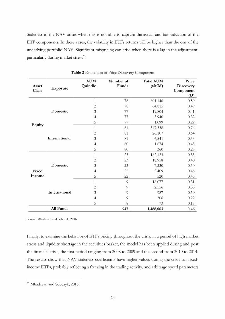
Mhadavan and Sobczyk define the price discovery component as the percentage of the total

variance that is not caused by transitory noise shocks. Table 2 reports the estimated statistics for

the price discovery element for both Equity and Fixed Income ETFs, distinguishing domestic from

international funds and splitting them by different sizes of funds AUM (in a range where 1 are the

largest and 5 are the smallest). We can see that the general components of the mispricing vary with

respect to the asset class, the exposure and the size of the ETF: on one hand, small and less actively

traded ETFs present a lower price discovery element, meaning that more than a half of their price

gap is due to non-fundamental reasons, on the other the 74% of the premium (discounts) variation

of big international equity funds is explained by the price discovery component. This confirms the

intuition of the two authors: for the biggest and most common funds in terms of trading, the gap

between NAV and ETF price is mostly a reflection of staleness in the first i.e. NAV pricing error.

52 Mhadavan and Sobczyk, 2016.

26

Staleness in the NAV arises when this is not able to capture the actual and fair valuation of the

ETF components. In these cases, the volatility in ETFs returns will be higher than the one of the

underlying portfolio NAV. Significant mispricing can arise when there is a lag in the adjustment,

particularly during market stress53.

Table 2 Estimation of Price Discovery Component

Asset Class

Exposure

AUM Quintile

Number of Funds

Total AUM ($MM)

Price Discovery

Component (D)

Equity

Domestic

1 78 801,146 0.59

2 78 64,815 0.49

3 77 19,804 0.41

4 77 5,940 0.32

5 77 1,099 0.29

International

1 81 347,338 0.74

2 81 26,107 0.64

3 81 6,541 0.53

4 80 1,674 0.43

5 80 360 0.25

Fixed Income

Domestic

1 23 162,123 0.55

2 23 18,958 0.40

3 23 7,230 0.50

4 22 2,409 0.46

5 22 520 0.45

International

1 9 18,077 0.31

2 9 2,556 0.33

3 9 987 0.50 4 9 306 0.22

5 8 73 0.17

All Funds 947 1,488,063 0.46

Source: Mhadavan and Sobczyk, 2016.

Finally, to examine the behavior of ETFs pricing throughout the crisis, in a period of high market

stress and liquidity shortage in the securities basket, the model has been applied during and post

the financial crisis, the first period ranging from 2008 to 2009 and the second from 2010 to 2014.

The results show that NAV staleness coefficients have higher values during the crisis for fixed-

income ETFs, probably reflecting a freezing in the trading activity, and arbitrage speed parameters

53 Mhadavan and Sobczyk, 2016.

27

are instead smaller. This could suggest that, particularly for less traded assets such as fixed income

securities, the price discounts to NAV during financial shocks reflects efficient pricing, bearing in

mind that ETFs price dynamics are always driven by their intrinsic arbitrage activity54.

2. EVIDENCES OF NON-FUNDAMENTAL SHOCKS PROPAGATION

As opposed to the view of Mhadavan and Sobczyk, other academics focus on the potential

transmission of non-fundamental shocks from the ETF to the underlying stock through arbitrage,

given that arbitrageurs take opposite position in the fund and its components55.

To study the impact of ETFs on financial markets, Malamud has created an equilibrium model that

makes it possible to analyze the ETF universe as a whole by allowing for any number of ETFs and

correspondent components. It pictures the creation and redemption mechanism as a shock-

propagation channel that, combined with APs’ arbitrage activity might create momentum in the

underlying assets returns and consequently lead to financial instability by reflecting temporary

demand shocks on future prices56. The requisite for this noise propagation is the presence of an

ETFs demand shock57.

If market would be efficient, we would expect the ETF price and its NAV to perfectly converge,

as reflections of the same exact fair value but unfortunately financial market has proven several

times not to be perfect. The continuous creation and redemption of new shares facilitates arbitrage

though, so that the two prices are not expected to diverge substantially. However, in the recent

years, ETFs have been increasingly employed for hedging and speculative aims that expose these

instruments to non-fundamental shocks. To this purpose, I. Ben-David, F. Franzoni and R.

Moussawi exemplify the propagation of shocks from the fund to its portfolio as follow. We imagine

an initial situation where neither premium nor discount exist between the ETF price and its NAV,

i.e. they have the same value, as shown in Figure 2.A. At one point, we suppose an exogenous

liquidity shock not based on any fundamental reason happens, for example a boost in the ETFs

54 Mhadavan and Sobczyk, 2016. 55 Da and Shive, 2017. 56 Malamud, 2015. 57 David, Franzoni and Moussawi, 2017.

28

shares demand by a large institution, positively influencing the ETF price (Figure 2.B). Arbitrageurs

suddenly steps in to take advantage of the mispricing, betting on the realignment of the two prices

by going short on the ETF and taking a long position in the underlying portfolio. This mechanism

triggers the shock spreading, making the price of the underlings increase (and consequently the

ETF NAV) and, at the same time pushing downward the ETF price as in Figure 2.C, until the

equilibrium in re-established. Eventually, the liquidity inflows received come back to normality and

both prices revert to their fair values, shown in Figure 2.D.

Figure 2 Non-Fundamental Shock Propagation

Source: David, Franzoni and Moussawi, 2012.

As we explained before, when ETF price experiences a shift with respect to its fundamental value

we can’t exclude the price discovery potential it bears. In fact, if the initial shock was happening

for a fundamental reason, ETF NAV would be moved by the same price-contagion as it is shown

in Figure 3. The initial equilibrium is broken by a shock in the fundamental value of the fund

portfolio; as mostly happens, the ETF market is more liquid with respect to its underlying market

2.A Initial equilibrium. 2.B Non-fundamental Shock to ETF.

2.C The non-fundamental shock is

propagated to the NAV through arbitrage,

the ETF price starts reverting to the

fundamental value.

2.D Re-establishment of equilibrium after

some time, both the ETF price and the NAV

revert to the fundamental value

29

so it comes with no surprise the chance of it making the first step towards the new fair value and

its NAV moving with a delay58.

Figure 3 Fundamental Shock with Price Discovery Occurring

Source: David, Franzoni and Moussawi, 2012

Given this potential, it’s necessary to demonstrate that the shock triggering the mispricing with

respect to the NAV comes from a non-fundamental initial shock. To do so, the authors decided

to create two further constraints: firstly, they show that the mispricing impact of a shock on the

NAV is short-lived, according with the fact of the shock being non-fundamental, secondly, they

expect the demand pressure on the ETF to not match the one on the underling portfolio.

Moreover, it’s essential to demonstrate that the underlying security wouldn’t be hit by the shock

propagation with the same intensity in the absence of ETFs, since we are trying to identify their

inner arbitrage activity as a shock-propagation channel. For this reason, the three authors reported

evidence that these funds, given that they provide low cost liquidity, attract short-term investors

58 David, Franzoni and Moussawi, 2012.

3.A Initial equilibrium. 3.B Shock to the fundamental value.

3.C The ETF price moves to the new

fundamental value. 3.D After a delay, the NAV catches up

with the new fundamental.

30

who enhance the possibility for liquidity shocks to happen and they access indirectly the underlying

components through the ETF intermediation.

To test their hypothesis, David, Franzoni and Moussawi used a sample of 1.146 ETFs in a time

frame going from September 1998 to March 2011. The fundamental measure used as ETF arbitrage

profitability is the mispricing i.e. the difference between ETF price and its NAV.

It’s quite straightforward to look at the behavior of the daily percentage mispricing observed in the

SPY during the analyzed period, showed in Graph 10. First, we notice a gradual shrinking in the

gap between the two values, probably as a reflection of increased liquidity in the ETF market (due

to increase AUM over time) and consequent lower transaction costs which made ETF arbitrage

more convenient. Second, the mispricing increases during period of market stress as the 2008-2009

financial crisis showing an intuitive relation with the overall market liquidity: lower levels of

liquidity might be a symptom of lower funding liquidity that in turn implies a reduction in the

capital invested in the ETF and make arbitrage less convenient as the transaction fees get higher.

Graph 10 Daily Percentage SPY Mispricing 1998-2011


To support the “clientele effect” assumption, the authors need to demonstrate two subsequent

phenomena. In the first place, ETFs ownership needs to show a decrease in the investors trading

0,02

0,01

0,00

-0,01

-0,02

-0,03

1998 1999 2000 2001 2002 2003 2004 2005 2006 2007 2008 2009 2010 2011

31

horizon than the ones investing in common stocks. Using the churn ratio of institutional investors59

as proxy for ETFs investors turnover, they find evidence that the average turnover of these funds

investors is in fact higher than the normal stocks. Then, they investigate on the effect of ETFs

ownership on the stock-level investors turnover and their results support the conjecture that ETFs

increases arbitrage activity between them and their underlings, consequently attracting shorter-time

horizon investors.

Now, focusing more on the shock propagation potential, we need to find a significant relationship

between the ETF mispricing and the movement in the NAV. In fact, if ETFs are representing a

channel for shock transmission to their underlings through arbitrage activity, we expect the ETFs

fundamental value to move in the same direction of the mispricing i.e. if positive investors are

expected to start buying the underlying and selling the ETF, if negative all the way around. In order

to test this hypothesis, a regression of a NAV day-t return against the mispricing in day-t-1, with

other control variables as date fixed effect has been made. The results are in line with what

expected: independently from the fund fixed effect control, the NAV return has a positive

coefficient with respect to the mispricing variable; in particular, a 1% gap between the ETF price

and its fundamental value is associated with an increase of 16 bps increase in the next-day NAV

daily return.

As we explained above, we also expect the arbitrage activity to cause a movement in the ETF price

exactly opposed to the mispricing. For this reason, the authors decided to regress ETF returns

against the prior day mispricing. Again, the negative coefficients support the conjecture and they

have a greater magnitude than the previous regression: a mispricing in day-t-1 will cause both the

fundamental value and the price of the ETF to move in a direction consistent with closing the gap,

the latter will move faster though, probably due to higher liquidity in the ETF market and to a

greater sensibility to liquidity shocks in comparison to the underlying market.

Finally, we need to rule out mispricing hasn’t been caused by fundamental shocks. If not, it would

mean that the ETF arbitrage activity would only be beneficial as a channel for price discovery. To

do so, the authors developed two more constraints: if the shock is non-fundamental, we first should

expect a reversal in the fundamental value during the following days as liquidity is expected to flow

59 Computed as the sum of quarterly absolute changes in dollar holdings over average assets under management.

32

back to a normal level.; second, the demand for the ETF should diverge from the demand of its

component when the shock hits the fund market only.

The vector auto-regression analysis is applied both to the NAV returns as a function of lagged

mispricing and NAV returns up to the 5th lag in order to investigate the length of the mispricing

impact on the NAV. The mispricing is observed to positively influence the fundamental value of

the ETF in the first lag. However, the NAV is negatively correlated with the mispricing when we

move to further lags. In particular, the authors noticed that the magnitude of the negative

correlation with the second lagged mispricing counterbalance the effect of the first i.e. the effect

of the initial shock, going from the ETF price to its NAV, is reverting on the second day.

Graph 11 replicates the behavior from the regression coefficients. It shows that, a shock to the

ETF price on day 0, that translates into mispricing, positively impact the NAV returns on day 1

but it’s counterbalanced by opposed movement on days 2 and 3.

Graph 11 Impulse Response Functions of a Shock on Future NAV Returns.

The grey bars represent two standard errors around the estimates. Source: David, Franzoni and Moussawi, 2012.

Then, to investigate about the discrepancies between buy and sell pressures between the ETF

market and its components, in order to identify non-fundamental shocks, the authors compare the

buy-sell order imbalance (OI) of the two markets. When the OI is positive there will be pressure

exercised by the bidding side, on the other hand, when negative there will be selling pressure. The

OI is computed daily for the ETF market, the measure is calculated as the value-weighted daily OI

of the assets composing the fund for the underlying portfolio instead. The main assumption made

by the authors is that, large OI in the ETF market not matched in the underlying securities are

0 1 2 3 4 5 6 7 8 9 10 11 12 13 14 15 16 17 18 19 20

0,5

0

-0,5

33

synonym of a demand shock affecting only the former level and being consequently non-

fundamental.

First, large OI dummies are used in the first stage of a two-stages least squares regression in order

to identify the existence of a significant relationship between demand imbalances and mispricing.

The resulting coefficients shows that the gap between the ETF price and its NAV is positively (and

negatively) related respectively with positive (and negative) buy and sell imbalances and the effect

seems to be symmetric. The authors then use those estimates as proxies for mispricing in the 2SLS

second stage regression, where the dependent variables are the NAV returns and the ETF return

respectively, at t+1. The results show consistency with the OLS that previously has been applied:

the mispricing component originating from non-fundamental shocks in the ETF market

propagates the latter to the underlying securities level. Finally, the same OLS regression is applied

only to those observations which OI indicator equals 1. Again, the predictability is found to be

similar to the evidence we obtained from the whole sample.

The results obtained by David, Franzoni and Moussawi’s study support their theory, showing that

arbitrage activity is not only helping to keep the ETF price and its NAV aligned but it can represent

a risk for financial markets since it has the potential to move the price of correctly-valued securities

and consequently causing noise transmission and volatility in the underlings included in the ETF

portfolio60.

3. ETFS AS NOISE SPREADERS INTO THE UNDERLYING SECURITIES MARKET

In 2015, David, Franzoni and Moussawi carried out one additional study, investigating the effect

of ETF on the volatility of the securities comprised in their basket. In particular, they interrogated

whether the prices of securities owned by a high number of ETFs display greater noise in the prices

and their behavior tends to differ from a random walk. Since they represent the wider category, the

analysis is focused on plain vanilla ETFs that physically track US stock indexes.

They begin by demonstrating that ETFs are mostly held by noise short-term investors due to their

greater liquidity with respect to their components. To investigate on these liquidity differences,

they collected some statistics regarding the bid-ask spread percentage, the Amihud measure of price

60 David, Franzoni and Moussawi, 2012

34

impact61 and the daily turnover. For all the 660 US-Equity ETFs listed on the US Stock Exchange62,

each of the three measures is computed as the average of all the assets in the fund portfolio, on a

quarterly basis, and subsequently, the value-weighted mean is calculated according to the market

capitalization of each ETF. As we can see in Table 3, all the three measures prove that the ETF

market is more liquid than the related underlying securities: narrower bid-ask spread, smaller

Amihud ratio and higher daily turnover.

Table 3 Liquidity measures

Variable Quarters ETFs Stocks Difference t-stat

Bid-Ask Spread 52 0,003 0,005 -0,002*** (-3,518)

Amihud Ratio 52 0,002 0,008 -0,006*** (-9,702)

Daily Turnover 52 0,093 0,011 0,083*** (-13,462)


Following the Amihud and Mendelson’s clientele effects63, as in their precedent study, which states

that short-term investors are more interested in investing in financial instruments with higher

liquidity, they find out ETFs investors turnover to be 6.7% higher than their underlying portfolio.

Finally, the marginal investor of the ETFs sample is analyzed in comparison with the ownership

of all the common stocks accounted by the CRSP64. What is discovered is that not only institutional

investors represent a smaller portion (47,4%) of the ETF market than what they do in stocks

(62,1%), causing ETF ownership to be more skewed towards retail investors that are more prone

to act alike noise traders65; but the institutional presence tends to have higher turnover in the ETFs

than in the underlying, with hedge funds representing the fastest trading category.

The second hypothesis developed by the authors, and the one pillar of this work, is that ETFs do

add an additional level of demand, and subsequently volatility, to the stock market. To demonstrate

this proposition, as we anticipated before, they focused their attention on plain vanilla US domestic

long equity ETFs in a time frame going from 2000 to 2012. They included only those funds

61 The ratio of absolute return to the financial instrument dollar volume. This is a proxy for the illiquidity of the instrument, showing the daily price impact of one-dollar trading volume. 62 As of 2015. 63 Amihud, Yakov, and Mendelson, 1986. 64 Center for Research in Security Prices owns one of the largest historical databases in stock research. 65 Stambaugh, 2014.

35

investing in US equity stocks market primarily, excluding those investing in physical commodities,

futures, international or non-equity securities in general as well as those applying leveraged, short

or active strategies. The final sample comprises 660 ETFs listed in the US Stock Exchange.

The existence of a connection between ETFs ownership and the volatility in the underlying basket

is firstly tested through an OLS regression. The ETFs ownership of a stock is defined as the sum

of the investments values of all the ETFs trading that security, divided by its total market

capitalization. The stock volatility, computed as the stock daily returns standard deviation within a

month, is then regressed against the variation of ETFs stocks ownership, across both securities

and time. Moreover, in order to avoid the potential omittance of spurious variables with returns

volatility, different controls have been included. ETFs ownership mainly depends on three factors:

a single stock can be comprised in the basket of different indices and, in parallel, those indices can

vary their weighting schemes, in addition to changes in the ETFs asset under management over

time.

The index weighting strategy is the most exogenous element to our dependent variable. If the

weights do not move together with the stock market capitalization though, as in equally-weighted

indices, this could create a false relationship between ETFs ownership and volatility caused by the

correlation between stock size and volatility. To capture this effect, the logarithmic market

capitalization has been included in the regression together with proxies for stock size, liquidity,

returns predictors and time fixed effect.

Table 4 reports the results of the OLS regression of the daily returns volatility in a given month

against the ETFs ownership for those stocks at the end of the prior month. S&P500 and Russell

3000 stocks are regressed separately to see the variation of the interest depending on the firm size.

A positive and significant relationship is observed for stocks of both indices: for every unit of

increase (or decrease) in the ETFs ownership SD, the stocks returns daily volatility will increase (or

decrease) of about 13,2%, consistently with the authors hypothesis that ETFs add a layer of noise

to their underlying basket. Then, we notice that, for smaller stocks i.e. those included in the Russell

3000, the coefficient is lower, between 4,2% and 5,2%, showing a weaker relation.

This phenomenon can be explained with the concept of “optimized replication”. To replicate an

index, fund managers or investors in general, have two choices: either to fully replicate the index

by buying all the securities included in it (full replication) or to buy only those securities in the index

36

that are the most representative of it for their risk, correlation and exposure (optimization)66. As

we explained in the first chapter, arbitrage activity when ETFs prices diverge from their

fundamental values, can be conducted directly on the second market level without involving

creation and redemption activity but only buying (or selling) ETF shares and selling (or buying) the

underlying portfolio, waiting for the two prices to converge. Consequently, through optimization,

arbitrageurs don’t need to invest in the whole ETF basket portfolio, but they can only focus on the

larger and more liquid stocks, minimizing the transaction fees, in order to construct the replicating

portfolio.

Table 4 ETFs Ownership and Stock Volatility

Dependent Variable Daily Stock Volatility

Sample S&P 500 Russell 3000

(1) (2) (3) (4)

ETFs ownership 0,132*** 0,127*** 0,052*** 0,042***

(4,828) (4,700) (4,606) (3,784)

Log (Mktcap (t-1)) 0,048 0,038 -0,096*** -0,116***

(1,271) (1,010) (-3,799) (-4,550)

1/Price (t-1) 1,574** 1,502** 0,814*** 0,905***

(2,446) (2,343) (2,954) (3,291)

Amihud(t-1) -9,242 -3,037 0,195 0,305

(-0,604) (-0,206) (0,704) (1,087)

Bid-ask spread (t-1) -7,346** -7,215** -8,894*** -8,168***

(-2,085) (-2,041) (-2,989) (-2,723)

Book-to-Market (t-1) 0,531*** 0,530*** 0,332*** 0,325***

(9,162) (9,172) (9,539) (9,381)

Past 12-month return (t-1) 0,025 0,016 0,056*** 0,061***

(0,668) (0,430) (2,791) (3,051)

Gross profitability (t-1) * 0,454*** 0,493*** 0,032 0,042

(4,143) (4,400) (0,607) (0,788)

Index fund ownership 0,028** 0,021***

(2,287) (3,537)

Active fund ownership 0,062*** 0,060***

(3,884) (6,509)

Stock fixed effects Yes Yes Yes Yes

Month fixed effects Yes Yes Yes Yes

Observations 67.261 67.261 289.563 289.563

Adjusted R2 0,645 0,647 0,593 0,595

.***, **, * represent statistical significance at the 1%, 5%, or 10% levels, respectively. *Gross income scaled by total assets.


66 https://www.etf.com/etf-education-center/21038-how-to-run-an-index-fund-full-replication-vs-optimization.html?nopaging=1

https://www.etf.com/etf-education-center/21038-how-to-run-an-index-fund-full-replication-vs-optimization.html?nopaging=1

https://www.etf.com/etf-education-center/21038-how-to-run-an-index-fund-full-replication-vs-optimization.html?nopaging=1

37

Finally, to test if ETFs ownership is capturing more than the effect of the stock ownership by

institutional investors, in column 2 and 4, the variables related to the stock ownership by both

active and indexed mutual funds have been introduced (being these latter the most similar to

ETFs). As we see, the coefficients are still positive but with lower magnitude with respect to the

ETFs, which slope remains almost unchanged showing an independent and stronger relationship

with stocks returns volatility accordingly with the first hypothesis that ETFs are mostly held by

noise traders. As we expected, following what said in the last paragraph, the coefficient for smaller

stocks is no more statistically distinguishable with the ones related to mutual funds.

As we considered earlier in this chapter, increase volatility in stock prices is not always connected

to pure noise. If the presence of ETFs makes stocks prices to react more promptly to change in

fundamental through the arbitrage activity it means that the observed increased volatility connected

with these funds stocks ownership, it’s no more noise but price discovery. The authors distinguish

between fundamental and non-fundamental volatility.

In order to investigate this matter, they conduct a further OLS regression on the variance of ETF

ownership, this time using as dependent variable the Variance Ratio, a measure for price efficiency

consisting, for every stock i at time t, in:

𝑉𝑅𝑖,𝑡 = |𝑉𝑎𝑟(𝑟𝑘,𝑖,𝑡)

𝑘 ∗ 𝑉𝑎𝑟(𝑟1,𝑖,𝑡)− 1|

where the numerator is the variance of k-period stock returns within a time frame t and the

denominator is k times the variance of a single period returns in equal t. When markets are efficient,

we expect the ratio between the two variances to approach 1, since prices should behave like a

random walk, and so the VR to approach zero. So, if ETFs add non-fundamental volatility to their

underlying securities, we should observe an increase in the Variance Ratio of a stock with higher

ETFs ownership of that stock.

Since, as already discussed, stock prices can be affected by ETFs arbitrage activity intraday and

daily, as arbitrageurs act both in the primary and secondary market, the VR has been constructed

with 15-seconds frequency and 5-days frequency respectively. The results are shown in Table 5,

the same control variables applied in the previous experiment have been adopted. The evidences

point out that a significant and positive relationship does exist between ETF ownership the VR,

38

being, the behavior of stocks with higher ETFs ownership, departing from a random walk and so

including more noise. As we see the link is stronger at the intraday frequency and, consistently with

the coefficients in Table 7, smaller stocks are found to be less affected.

Finally, as the authors carried out in their 2012 experiment, we look for a mean-reverting

component in the stocks returns as we expect by Figure 2, when a demand shock happens in the

ETFs market, we expect the price of the underlying securities to move in the same direction, since

the fundamentals haven’t change though, the prices should revert to the initial level in the following

days.

Table 5 ETFs Ownership and Stock Volatility Variance Ratios

Sample: S&P 500 Russell 3000

Dependent Variable: VR 15 seconds VR 5 days VR 15 seconds VR 5 days

(1) (2) (3) (4)

ETFs ownership 0,109*** 0,049* 0,061*** 0,013

(4,485) (1,809) (7,620) (1,188)

Controls Yes Yes Yes Yes

Stock fixed effects Yes Yes Yes Yes

Time fixed effects Yes Yes Yes Yes Observations 56.623 22.887 268.418 100.836 Adjusted R2 0,473 0,032 0,488 0,041

***, **, * represent statistical significance at the 1%, 5%, or 10% levels, respectively. Source: David, Franzoni and Moussawi, 2015.

To investigate this hypothesis, the returns of the underlying securities, at different and overlapping

time horizons, have been regressed against the net flows of creations and redemptions in ETFs

made by APs. The values of the securities included in the basket should move according to the

ETFs flow no matter if due to fundamental or non-fundamental reasons. Assuming that at least, a

part of the initial shock is not justified by a change in fundamentals, we expect a price reversal to

happen in the next days. The previous control variables haven’t change.

For a one standard deviation change in the net flow, there is a contemporaneous movement of

16.7 basis points in the prices of the S&P 500 stocks. In the next days though, the negative

coefficients predict reversion in the stocks prices showing that at least half of the initial impact on

returns volatility is caused by noise propagation. Accordingly to the previous experiments, the

absolute value in the Russell 3000 stocks is smaller.

39

At this point, since we found evidences of an existing link between ETFs ownership and underlying

stocks non-fundamental volatility one question arises: are ETFs adding a new layer of demand to

their components, that wouldn’t be present without them, or they are reshuffling noise from stocks

with low ETFs ownership to stocks with a high one?

The argument for the first hypothesis is that these funds are providing trading low-cost and high

frequency opportunities which weren’t available before and consequently attracting new investors

and new strategies. On the other hand, the supposition that ETFs represent only a new, cheaper

channel for existing investors to trade the underlying securities is admissible as well. This last

argument could be easily applied also to futures and other derivatives; however ETFs give to

investors a broader range of market segment specialization.

The only way to test the two hypothesis is by evolution of ETFs ownership and volatility overtime.

If the hypothesis of the new layer of demand holds, we should see an increase of the stocks returns

volatility as they are included in the ETFs portfolios. The aggregate volatility is, instead, predicted

to be steady in case of the reshuffling hypothesis since ETFs shouldn’t change it.

The authors regressed the average daily volatility of all stocks included in CRSP, against the lagged

average ETFs ownership. To exclude the possibility that the estimates would be influenced by

institutional ownership, index and active funds activities are used as independent variables. A trend

is then used to capture all the developments in global conditions, reduction in trading costs as an

example. The new-layer-of-noise hypothesis is supported by the results: the inclusion of the stocks

in ETFs portfolios significantly and positively impacts their volatility.

Despite the evidences are found to be against the second hypothesis, the presence of a shift in

returns volatility from some stocks to others as the ownership of ETFs increases, it is not excluded.

To investigate on this possibility, stocks are divided in five different quantiles of ETFs ownership

(from 0,7% to 4%), for each of them the average monthly volatility is regressed on the average

lagged ETFs ownership and controls are included. In Table 6 we see that the volatility of all the 5

groups increases with ETFs ownership, excluding a noise reshuffling among stocks and that the

coefficient turns higher with increase in the lagged ownership, strengthening the causal association

between stocks prices noise and the inclusion in ETFs portfolios67.

67 David, Franzoni and Moussawi, 2015.

40

Table 6 Regression of Volatility and ETFs Ownership, by Quintiles of ETFs Ownership

Dependent Variable: Volatility(t+1)

Quintile of ETFs ownership Smallest 2 3 4 Largest

ETFs ownership(t) 0,189*** 0,213*** 0,206*** 0,216*** 0,247***

(3,532) (4,075) (3,890) (4,154) (3,856)

IF ownership(t) -0,063 -0,068 -0,049 -0,049 -0,093

(-1,062) (-1,144) (-0,823) (-0,863) (-1,381)

AF ownership(t) 0,025 0,060 0,091* 0,089* 0,150**

(0,497) (1,193) (1,799) (1,823) (2,560)

Volatility(t) 0,760*** 0,688*** 0,656*** 0,638*** 0,667***

(15,050) (12,508) (11,261) (10,779) (11,548)

Trend 0,000 0,000 0,001 0,000 0,002

(-0,027) (-0,238) (-0,606) (-0,183) (-1,216)

Observations 149 149 149 149 149

Adjusted R2 0,759 0,691 0,648 0,662 0,726

***, **, * represent statistical significance at the 1%, 5%, or 10% levels, respectively. Source: David, Franzoni and Moussawi, 2015.

4. COMMONALITY IN THE RETURNS PATTERNS OF ETFS UNDERLYING PORTFOLIOS

So far, thanks to the David, Franzoni and Moussawi’s researches, we found empirical evidences

that ETFs, through their shares creation and redemption mechanism and the related arbitrage

activity, represent a channel for non-fundamental shocks propagation into their underlying

securities market. As a consequence, it comes with no surprise that a causal relationship is found

to exist between the ETFs ownership of a stock and its returns volatility.

We deepen the subject by wondering if, since ETFs transmit the same shock to all their

components, they create commonality in the returns behavior of the assets included in the

underlying portfolio.

Wurgler, in his 2011 work, investigates the consequences of index-linked investing and finds

evidences that, with the spreading of passive investing, the market has become unable to absorb

index-shaped stocks demand.

The inclusion of a stock in the S&P 500 does not depend on its fundamentals or investment

potential, rather it is based on the liquidity of the shares and their market representativeness. Every

time a new stock is added to the Index, index funds managers tracking the S&P 500 must buy the

same percentage, no matter if the stock is overpriced. On average, the value of the securities added

41

to the Index between 1990 and 2005 has been observed to have increased about 9%, deleted stocks

have plunged even more. Intuitively, the basic explanation for this phenomenon relies on the

interactions between supply and demand. Even though a part of the increase in the prices could be

easily attributed to the expected increase n the stock liquidity, we need to remember that this latter

is one of the same reasons why the stock has been included in the Index portfolio; in addition,

mostly important, changes in liquidity proxies such as volume bid-ask spreads and quoted depths

are observed to be too small to justify such big price appreciations.

It is worth noticing that the same inclusion-effect has been observed for other indexes as well such

as the Russell 2000 and 1000, Nikkei 250, MSCI country indices and others68.

The most relevant evidence Wurgler observes is that, as soon as a new stock is included in the S&P

500, its returns pattern starts to change. The stock begins to behave more similarly to the other

securities included in the index portfolio, slowly drifting away from the market remaining part. As

a matter of fact, stocks included in the Index between 1978 and 1997 have been experiencing a

significant price premium in comparison to other comparable stocks in terms of size and industry,

kept out from it69.

Similarly to the prices jumps and falls, this is mainly related to the highly correlated money outflows

and inflows the stocks experience after their inclusion inside the index portfolio. In fact, the net

flows observed pouring into index-linked securities are not totally correlated to the other investors’

strategies: by definition they are different from the approaches applied by active investors, they are

more interested, for example, in the price parity between the Index derivative and its underlying

portfolio (i.e. index arbitrageurs) rather than simply tracking the relative index and no-index stocks

valuations. Overtime this creates a common trend that causes the index members to move more

closely while detaching from the non-members70

Given these evidences, we proceed investigating the role that ETFs play in this scenario given that

ETF arbitrage has a higher probability to drive returns commovement in the underlying portfolio

than other correlated money flows. In fact, taking position on both the ETF and the underlying

stocks, arbitrageurs might cause the securities prices to move in the same direction, creating a

common exposure different from the assets fundamentals71.

68 Wurgler, 2011. 69 Morck and Yang, 2001. 70 Wurgler, 2011. 71 Da and Shive, 2017.

42

Da and Shive carry out a thorough analysis regarding the existing link between ETFs ownership

and the return commovement among the assets included in their portfolios. In a time frame going

from July 2006 to December 2013, they use a sample of 549 US plain equity ETFs and 4.487 stocks,

of which 4.318 are held at least by one ETF during the period. The shares belong to firms having

a minimum of 100$ million market capitalization and a price per share of 5$ or greater. The ETFs

are observed to hold, on average, the 0.113% of their underlying baskets market capitalization, that,

if considered together, adds up to a distinctive part of them. It is worth to notice that the average

ETFs turnover is 3%, showing much more liquidity than the stocks do, whit a mean of 1% daily.

Moreover, the authors compute a variable called N. Holdings, that is represented by the stocks in

the ETFs portfolios that matches with the ones in the stocks sample and on average counts to 261

stocks.

To conduct this research, different measures are used. First, the authors construct a measure for

the average correlation of stocks comprised in an ETF portfolio. This is called Fratio (Fund Level

Variance Ratio), is computed monthly and consists in the ratio between the variance of the average

underlying stocks daily returns and the average of the variances of the underlying stocks daily

returns. Then they use three proxies for the ETFs activity at the portfolio level: Holdings% as the

proportion of the underlying basket held by an ETF, SD Shares (the standard deviation of the daily

outstanding ETF shares divided by the monthly average outstanding shares) capture the intensity

of the ETF creation and redemption activity, providing a linkage to the demand volatility the

underlying stocks and ETF Turnover that is the monthly average ratio of the fund shares traded and

the shares outstanding during a specific day.

They start by regressing the Fratio on ETFs activity measures to investigate which is the variable

affecting the portfolio stocks correlation the most. Time and funds fixed effects are used to capture

the effect of elements such as industry, market return and volatility (columns 1 to 4) in addition to

the introduction of an interaction term between the two (columns 5 to 8); this latter is used to

address the concerns that stocks might experience an increase in correlation due to their

fundamentals, since ETF activity has been increasing over all the sample time period this could

create a spurious relationship between the two terms.

Table 7 shows the computed coefficients. We see that SD Shares is always non-significant while

Holding% becomes when the interaction variable is introduced.

43

Table 7 Regression of Fund Level Variance Ratio

Dependent Variable Fratio

(1) (2) (3) (4)

Holdings% 0.0381*** 0.0417***

(0.0131) (0.0135)

SD Shares 0.0212 −0.0204

(0.0215) (0.0237)

ETF Turnover 0.145*** 0.155***

(0.0325) (0.0358)

Expense Ratio −2.776 −2.777 −2.449 −2.421

(2.057) (2.049) (2.085) (2.084)

Log(TNA) −0.00507** −0.00336 −0.00346 −0.00533**

(0.00251) (0.00259) (0.00254) (0.00246)

Log(Nholdings) −0.0559*** −0.0562*** −0.0559*** −0.0555***

(0.00950) (0.00947) (0.00945) (0.00947)

Time FE YES YES YES YES

Time FE*Fund NO NO NO NO

Fund EE YES YES YES YES

Observations 23,813 23,813 23,813 23,813

R2 0.748 0.7638 0.765 0.7655

(5) (6) (7) (8)

Holdings% 0.0116 0.00987

(0.0160) (0.0155)

SD Shares 0.0103 0,0261

(0.0221) (0.0240)

ETF Turnover 0.140*** 0.147***

(0.0302) (0.0322)

Expense Ratio 6.274*** 6.199*** 7.042*** 7.134***

(2.228) (2.244) (2.194) (2.178)

Log(TNA) −0.00478 -0.00431 -0,00418 -0,00458

(0.00448) (0.00436) (0.00427) (0.00440)

Log(Nholdings) −0.0591*** -0.0591*** -0.0589*** -0.0589***

(0.00852) (0.00852) (0.00848) (0.00848)

Time FE YES YES YES YES

Time FE*Fund YES YES YES YES

Fund EE YES YES YES YES

Observations 23,813 23,811 23,813 23,813

R2 0.7863 0.7863 0.7864 0.7865

***, **, * represent statistical significance at the 1%, 5%, or 10% levels, respectively. Source: Da and Shive, 2017.

Rationally, it’s not surprising that ETFs shares creation (and redemption) is observed to be less

significant from the moment that it doesn’t requires the trading of the basket. ETFs turnover, as

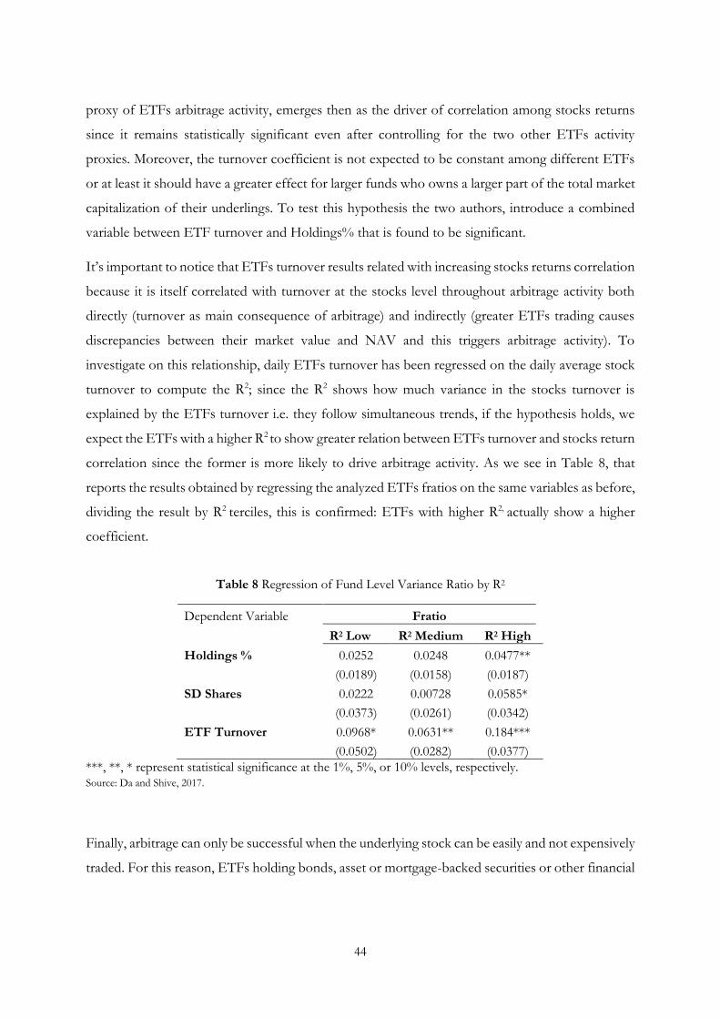
44

proxy of ETFs arbitrage activity, emerges then as the driver of correlation among stocks returns

since it remains statistically significant even after controlling for the two other ETFs activity

proxies. Moreover, the turnover coefficient is not expected to be constant among different ETFs

or at least it should have a greater effect for larger funds who owns a larger part of the total market

capitalization of their underlings. To test this hypothesis the two authors, introduce a combined

variable between ETF turnover and Holdings% that is found to be significant.

It’s important to notice that ETFs turnover results related with increasing stocks returns correlation

because it is itself correlated with turnover at the stocks level throughout arbitrage activity both

directly (turnover as main consequence of arbitrage) and indirectly (greater ETFs trading causes

discrepancies between their market value and NAV and this triggers arbitrage activity). To

investigate on this relationship, daily ETFs turnover has been regressed on the daily average stock

turnover to compute the R2; since the R2 shows how much variance in the stocks turnover is

explained by the ETFs turnover i.e. they follow simultaneous trends, if the hypothesis holds, we

expect the ETFs with a higher R2 to show greater relation between ETFs turnover and stocks return

correlation since the former is more likely to drive arbitrage activity. As we see in Table 8, that

reports the results obtained by regressing the analyzed ETFs fratios on the same variables as before,

dividing the result by R2 terciles, this is confirmed: ETFs with higher R2, actually show a higher

coefficient.

Table 8 Regression of Fund Level Variance Ratio by R2


R2 Low R2 Medium R2 High

Holdings % 0.0252 0.0248 0.0477**

(0.0189) (0.0158) (0.0187)

SD Shares 0.0222 0.00728 0.0585*

(0.0373) (0.0261) (0.0342)

ETF Turnover 0.0968* 0.0631** 0.184***

(0.0502) (0.0282) (0.0377)


Finally, arbitrage can only be successful when the underlying stock can be easily and not expensively

traded. For this reason, ETFs holding bonds, asset or mortgage-backed securities or other financial

45

instruments hard to be traded quickly, should not see increase returns correlations in their basket

securities.

121 ETFs having such financial instruments in their baskets have been selected and the same

regression has been applied to them and as we were expecting their turnover coefficient is no more

statistically significant as it shown in the second column of Table 9. A full sample and one

comprising mostly stocks are presented as well.

Table 9 Regression of Fund Level Variance Ratio by Basket Securities


Full Sample Bond > 0 Common ≥ Median = 99,67%

Holdings % 0.0417*** 0.0780 0.0168

(0.0135) (0.102) (0.0194)

SD Shares −0.0204 −0.244* −0.0135

(0.0237) (0.125) (0.0258)

ETF Turnover 0.155*** -0.0705 0.174***

(0.0358) (0.300) (0.0456)

Expense Ratio −2.421 113.0 −0.714

(2.084) (74.10) (2.595)

Log(TNA) −0.00533** −0.00707 −0.00409

(0.00246) (0.0151) (0.00273)

Log(Nholdings) −0.0555*** −0.0206 −0.0566***

(0.00947) (0.0268) (0.01000)

Time FE YES YES YES

Fund FE YES YES YES

Observations 23,813 1,230 12,613

R2 0.7655 0.7199 0.7554 Avg abs(gap) 0.0022 0.0054 0.0019


It is worth noticing that for all the ETFs having their baskets made by more than the 99,67% of

stocks, their arbitrage activity has a greater influence on their stocks returns correlation. The last

row reports the average discrepancy between the NAV and the market value of the ETFs during

the period. As a consequence of the limits-to-arbitrage, the gap is higher for the fixed income-

46

bearing ETFs, this might suggest that higher discrepancies rather than showing arbitrage

opportunities, they show arbitrage difficulties72.

5. FROM PHYSICAL TO SYNTHETIC ETFS

So far, we have mainly analyzed the effect ETFs activity has on the underlying baskets of securities.

We found evidence that the arbitrage activity APs and common investors carry out both on the

ETF and stock market levels, in order to keep ETFs market value and NAV aligned, has potential

to cause noise on the underlying stocks propagating non-fundamental shocks and, at the same time

causing pattern of commovement in their returns. The effect is even more accentuated when large

ETFs are involved, and the stocks are more liquid.

In the first chapter, we explained how ETFs can be differentiated by the replication method they

use to track the underlying portfolio behavior. Physical ETFs hold the securities they are trying to

mimic in their portfolio, the APs usually give (or receive) the underlying asset in exchange of the

fund shares. Fund manager though, can also decide to replicate the behavior of a certain index,

stock or similar without physically owning the securities. Synthetic ETFs usually takes derivatives

positions like a total return swap agreement with a financial institution that has the contractual duty

of delivering the return on the benchmark to the ETF73.

Figure 3 Unfunded Swap ETF Structure.

Source: Ramaswamy, 2011

72 Da and Shive, 2017. 73 Malamud, 2015.

47

Alternatively, in Figure 4 the funded swap structure is pictured. The ETF sponsor delivers cash to

the swap counterparty, which won’t receive further cashflows, and the received collateral basket is

kept in a segregated account created with an external custodian on which the fund has legal claims.

Since the ETF is not the beneficial owner of it, the sale of the basket securities in case of swap

counterparty default can be affected by delays74.

While physical ETFs investors are exposed to a tracking error risk, synthetic ETFs are subject to a

different one. In this latter replication scheme, it’s the swap counterparty assuming the risk of any

deviation of the ETF return from its benchmark and, as a consequence, investors in the ETF bear

the risk of the counterparty default75.

Figure 4 Funded Swap ETF Structure

Source: Ramaswamy, 2011.

When selling synthetic ETFs shares, usually ETF sponsors try to highlight the lower tracking error

without excessively focusing on the counterparty risk. Moreover, they emphasize the greater

cheapness with respect to the ones employing physical owning the security. The spreading of ETFs

popularity among investors and the recent decline in the investment funds expense ratios is causing

74 Ramaswamy, 2011. 75 David, Franzoni and Moussawi, 2017.

48

the competition in the sector to rise, pushing ETFs managers to employ different replication

methods in order to optimize the fund fee structure.

Indeed, one of the reasons for the choice of using a synthetic replication schemes is cost efficiency.

Physical replication might be optimal when dealing with indices focused on a specific market sector

and/or region which present a good level of liquidity and are widely traded. On the other hand,

this might become expensive for broader segments like emerging market or fixed income indexes

since their underlings might be harder to trade, less liquid and costlier. In those circumstances,

synthetic replication becomes a cost-efficient tracking method76.

An additional reason to use these replication methods is that they allow to exploit possible synergies

between the ETF sponsor and its swap counterparty, i.e. the investment banking division of the

parent bank and its asset management department. Investment banking activities require the bank

to set aside a large amount of stocks and bonds for mark-to-market purposes and they need to be

funded; when they are particularly illiquid though, the bank has no choice but funding them either

in the unsecured or repo market, with high haircuts. If the bank is able to transfer these securities

as collateral to its sponsored ETFs, the investment banking division might benefit from a reduction

in warehousing costs and part of this advantage can be transferred to the ETF investors as well,

through lower total expense ratios.

Unfortunately, there might be incentives to give as collateral illiquid assets since, as we said, the

bank can efficiently fund them with no extra costs and, if when the unfunded scheme is employed,

it may benefit also from lower regulatory capital requirement. Regulations over liquidity standards

like the ones introduced by Basel III might further push banks to use these practices. As an

example, the new requirements on the Liquidity Coverage Ratio introduced in 2015 requires banks

to hold highly liquid assets counting for 100% (as cash, treasuries and corporate bonds) of their

net cash outflows over a 30-days stress period and unsecured and secured funding backed by either

illiquid or low credit rating assets maturing over this period are comprised. If the financial

institution decides instead to use them as collateral in a swap ETF contract, which typically will

have a duration greater than one year, they will need a coverage only about the 20%.

The increasing use of synthetic replication schemes in ETFs and the greater complexity of these

products might create risks for financial stability. First of all, we need to remember the main risk

exposure difference between synthetic and physical replication. In fact, as we said, the former

76 Ramaswamy, 2011.

49

transfer the tracking error to the swap counterparty, who has to deliver the total return of the

benchmark to the ETF. Nowadays there exists low transparency on the methods used by the

financial institution to deliver the contractual cashflow to the fund but they usually create an

optimized representative subset of the securities included in the tracked index i.e. physical

replication. This means that the bank entering in this this financial contract is not only exposed to

the general trading book risk but to the tracking risk as well, potentially undermining its financial

stability if not well managed. Since ETFs cannot restrict investors redemptions when markets are

low in liquidity, we also need to consider the potential issues that the institution would incur in

providing the liquidity needed when large ETFs withdrawals happen suddenly, meanwhile keeping

the tracking risk under control77.

While the tracking error is transferred to the bank, the ETF sponsor is still exposed to the

counterparty risk. In period of crisis or general counterparty risk spreading, large institutional

investors might be encouraged to withdraw their investments from synthetically replicated ETFs.

This happens because the collateral basket used by banks usually heavily diverge from the one

composing the ETF benchmark and, as we explained before, swap counterparty might have

incentives to include illiquid assets in it. Moreover, institutional investors have been observed to

be the first market participants to exit when crisis happen, possibly triggering general panic when

fund solvency is doubtful and raising correlation among securities: while banks might be forced to

sell assets included in the collateral basket, APs might start asking for ETFs shares redemption in

order to provide liquidity to the market, setting a loop further undermining the counterparty

solvency.

Funding risk might come along with large investors withdrawals and increasing default risk: swap

ETF arrangements are considered by banks cheap ways to access funds from the moment that final

investors are not provided with the liquidity they have been promised. When redemptions take

place, cash is needed to be given back to the investors in exchange for the collateral basket that

might be not as easily marketable as expected. Since market makers could be prone to give more

relevance to these funding activities rather than accomplished their responsibilities to maintain

liquidity and fairness in the financial markets aggregate risk might be enhanced by a collapse in

financial intermediaries access to funds and consequent reinforcement of financial system funding

stress.

77 Ramaswamy, 2011.

50

Finally, the common perception of ETFs market as liquid can lead investors to underestimate the

market risk deriving from the increasing complexity of these products and the creation of options

and leveraged instruments on them. In fact, when employing synthetic replication methods,

products transparency decreases since different players and markets start to get involved and risk

monitoring ability decreases, leaving the final investors with low clarity on the replication

mechanics of the ETF bought78.

6. SYSTEMIC RISK ENHANCEMENT

Different episodes in the past years have triggered regulators attention towards ETFs and the risk

they may represent in periods of market stress. The main concern is that these financial products

may be a channel for liquidity shocks spreading among their underlying securities.

Investors are interested in ETFs for all the low-cost diversification opportunities that they offer.

In particular in the last years, where interest rates have been through a low-phase, these funds have

not only been used for investing in the classic liquid equity market, but also to gain exposure to

less traded securities like fixed-income securities, municipal bonds and emerging markets products.

As we have seen in the precedent paragraphs, ETFs might have a mixed effect on market liquidity,

hanging from price discovery conduits for their components by providing a market price for them

in times of poor liquidity, to serve as accelerators for volatility spreading throughout the market

during periods of market instability. When securities prices information is not reliable, or arbitrage

is found out to be too costly, market makers and arbitrageurs are likely to exit the market ceasing

the intermediation activity and causing more illiquidity in their underlying portfolios markets,

shocks amplification and spreading.

This is demonstrated by several episodes in the recent history, where arbitrageurs didn’t find

incentives to enter the market during stressed periods and this consequently led to big mispricing

between ETFs and their NAV.

During the Flash Crash happened in May 2010 for example, the S&P 500 sank roughly the 9% in

20 minutes, probably caused by the spreading of the unusual volatility that was before detected in

the S&P 500 future contracts. On that day, the anticipation of news about the Greek debt crisis

prompted institutions to sell the ETFs shares they were owning; at the same time, ETFs

78 Ramaswamy, 2011.

51

arbitrageurs stepped in with the aim of buying the ETFs shares and selling the underlings.

Unfortunately though, liquidity shortages in some exchanges caused the prices data to be not

reliable enough, leading arbitrageurs to exit the market and boosting the exacerbation of the market

turbulence. During those 20 minutes, ETFs market liquidity dried up and price discovery ceased

to occur, causing large discrepancies between ETFs market price and the prices of their

components79.

Volatility can affect the ability to trade ETFs as well. For example in June 2013, the Federal Reserve

Chairman raised fears about the approaching of the end of Quantitative Easing causing a general

and heavy sell-off. Here, one ETF decided to allow only in-kind redemption, since the transaction

fees applied to cash transactions i.e. cash redemptions, were so high to exceed the expense limit it

had for that day; moreover, other APs couldn’t keep transmitting redemption orders since they had

reached internal net capital limits. These events caused a break on the arbitrageurs’ activity and

ETFs prices to fall under investor selling pressures80.

After the Flash Crash of 2010, the SEC decided to introduce an inhibition to trade on single

securities, ETFs included, when they are facing period of extreme prices swings. On the 24th of

August 2015, this ruling caused the shares of more than 300 ETFs to stop trading: market makers

and APs exited the ETFs market after a trading halt on futures that faced steep declines before the

market opening and that these market participants were used to employ as hedging instruments

during volatile markets sessions. On that day, the trading volume of ETFs was representing the

42% of the total US Equity Market and the shock hitting their prices was eventually spread to their

underlings without any fundamental reason81.

Different studies analyzed in this chapter have shown evidences that movements in the ETFs

market price do influence the value of their portfolio components. The arbitrage activity performed

by investors to exploit the price differences between ETFs market value and their portfolios

components prices doesn’t always serves as price discovery instruments. We saw how market

shocks in the former can be easily propagated to the latter through arbitrage activity, even when

fundamentals are not involved, eventually reversing on the second next trading day but still

increasing prices movements and so market volatility. This non-fundamental shock propagation is

further enhanced by the commovement between ETFs underlying assets. Indeed, Da and Shive

79 David, Franzoni and Moussawi, 2017. 80 Office of Financial Research, 2013. 81 David, Franzoni and Moussawi, 2017.

52

research showed that the prices of securities held by ETFs tend to display commonality in their

returns over time.

Due to the increasing use of exotic ETFs and synthetic replication methods, when talking about

ETFs, counterparty and solvency risk need to be considered, together with the level of transparency

of the financial product delivered to the final investor.

53

III. EVIDENCES FROM FLASH CRASHES

As we anticipated before, the 6th of May 2010 equity-based securities in United States have been

hit by a fast and steep decline in prices that took their quotation to lose from 5% to 10% of their

values in approximately 20 minutes and eventually reversed by the end of the trading day. The

Securities and Exchange Commission estimated that among approximately 300 financial

instruments, roughly 20.000 trades got carried out with prices differing more than 60% from their

values some minutes before.

Among all the affected instruments, ETFs have been identified as the one category whose prices

dropped the most. According to the “clearly erroneous execution rules”, the SEC can cancel trades

that, under its examination, have been submitted by fault. From 14:40 and 15:00, out of 326 broken

trades, 70% of them were composed by ETFs. As we can see by Table 10, which shows the trades

involving ETFs in that time interval, approximately 96% of ETFs shares exchanged experienced a

loss between 0 and 10% with respect to their quotation at 14:40. 3 million of them though, showed

losses accounting for the 90-100% of the initial values. 160 ETFs lost almost their total value with

respect to their closing price on May 5th, considering the lowest transaction price executed on May

6th82.

Table 10 ETFs Trade Executed at a Loss

Total Trades

Total Volume

Total Volume ($)

All Trades 1.265.637 456.335.890 22.381.572.444

Losses 794.607 279.836.213 14.135.649.267

0% to -10% 761.866 269.307.656 13.909.304.917

-10% to -20% 13.607 3.988.959 145.247.171

-20% to -30% 3.714 1.144.431 40.234.001

-30% to -40% 2.041 753.856 18.934.582

-40% to -50% 1.151 320.661 6.612.612

-50% to -60% 1.148 344.774 7.657.548

-60% to -70% 758 314.03 4.111.592

-70% to -80% 505 233.617 2.021.741

-80% to -90% 775 176.632 1.025.499

-90% to -100% 9.042 3.251.597 499.604

Source: SEC and CFTC, 2010 (B).

82 SEC and CFTC, 2010 (B).

54

Looking at Graph 12, we see the timing of the daily lows of these instruments. In contrast with all

the other securities, which daily lows were experienced more heavenly during the one-hour

timeframe, the highest frequency for ETFs is reached from 14:45 and on: the blue line is composed

by all the ETFs losing their total value at their daily lowest price83.

Graph 12 Timing of ETF Daily Lows from 2 to 3*

*Daily Lows are computed with respect to the May 5th closing prices.

Source: SEC and CFTC, 2010 (B).

1. THE TRADING DAY

The trading day in U.S. markets started more volatile than usual due to some unanticipated political

and economic news concerning European sovereign debts and Greece potential default. To hedge

against this scenario, to be willing to take more risk, investors started to ask for higher premiums

on a different number of securities e.g. credit default swaps on different sovereign debt securities

in Europe84.

83 SEC and CFTC, 2010 (B). 84 SEC and CFTC, 2010 (A).

14:00 14:05 14:10 14:15 14:20 14:25 14:30 14:35 14:40 14:45 14:50 14:55 15:00

20%

0%

-20%

-40%

-60%

-80%

-100%

-120%

Retu

rn (

%)

55

Financial markets started to experience a “flight to quality” meaning that investors began to sell

what they were feeling to be riskier investments in order to purchase safer securities like gold and

U.S Treasuries: gold futures quotation rose about 2,5% and the 10-years U.S. Treasuries yields

plunged 5%. At the same time, the VIX saw his fourth highest spike of about 31,7%.

The overall turbulence started to spread to equities prices as well, triggering a number of Liquidity

Replenishment Points (LRPs)85 on quoted NYSE single stocks above average.

Derivatives instruments on the S&P 500 were affected as well. In particular, the liquidity on the

most actively traded products based on the index, namely the futures contracts on the S&P 500,

the “E-Mini”, and the SPY, experienced a draining on their buy-side liquidity plummeting 55%,

from $6 to $2,65 billion, for the former, and 20% for the latter, from $275 to $220 million.

Around 14:32, a large institutional investor input a selling order in the market to sell 75.000 June

2010 E-Mini contracts in order to hedge against the drop in equities prices. The automated

execution algorithm set to sell them was arranged with no instructions regarding neither the price

nor the time but only to respect an execution rate of 9% the trading volume observed the minute

before.

The order was executed extremely rapidly in about 20 minutes, a very short time considering that

such big trades are usually carried out in one whole trading day. At first, the orders were absorbed

by high frequency traders, fundamental buyers and cross-market arbitrageurs and the trading

volume increased, so the automated trading program sped up placing orders even though the

previously sent hadn’t yet been executed.

In about 3 minutes, from 14:41 to 14:44 the price of the E-Mini sank of 3% meanwhile arbitrageurs

who initially bought the futures contracts started to sell an equivalent quantity on the equity markets

in order to profit. Consequently, the selling pressure was spread to the SPY that in turn lost 3% of

its initial value86.

The volumes started to move faster so that in 15 seconds 27.000 E-Mini contracts (49% of the

total volume traded) were exchanged by HFTs that started to sell and re-buy the securities between

each other, due to the lack of buyers. The liquidity depth of the demand for the future contracts

85 LRPs are defined as volatility breaks. They are triggered when the price of a trade on a security hits predetermined lower or higher threshold with respect to the trading price. On this occasion, the Exchange will pause in order to make more liquidity to flow in the market. 86 SEC and CFTC, 2010 (A).

56

decreased to less than 1% of its morning level and the prices additionally sank of 1,7% in the same

time-period. The SPY plummeted of 6% from 14:41 to 14:45 and the net liquidity imbalance on

the futures contract was computed to 30.000 contracts for the selling side.

Finally, to avoid further dips in the prices, the Chicago Mercantile Exchange stopped the trading

on the E-Mini for 5 seconds at 14:45:28. The selling pressure started to relax while the buyers

slowly re-entered the market so that when the trading started again, both the E-Mini and the SPY

began to recover.

At the same time, the liquidity shock was spread to equities. Due to the steep drop in prices, many

automated trading systems of different actors in the market stopped in order to let the participants

to evaluate the convenience of staying in the market. As a result of their risk analysis, many market

makers decided either to exit, to decrease the liquidity made available or to increase their bid-ask

spreads.

The buying interest on individual stocks and ETFs started to decline despite the recover in the SPY

and E-Mini, so that the selling pressure drag the prices further down. In twenty minutes, from 2:40

to 3:00, $56 billion were traded accounting for almost 2 billion of shares and the 98% of them with

quotes within 10% down of their price before the decline.

For some individual securities (including ETFs), liquidity completely disappeared and orders to

either buy or sell at the market, finding no counterparty, were executed at absurd prices resulting

from stub-quotes. Indeed, stub-quotes are prices set by market makers to be far away from the

current quotes and they are not intended to be executed; liquidity providers issue these quotes in

order to respect their duty of providing continuous quotations for both sides, even though they

exited the market.

As a result, the execution of trades at these unrealistic prices triggered different LRPs from the

stock exchange, resulting in a notable number of broken trades87.

Eventually, at 15:00, both buyers and sellers came back in the play and price discovery started to

work again, reverting the quotations to normal levels. In that 20 minutes time-range, investors

bought and sold over 300 securities in 20.000 trades. As we will see, it’s important to highlight that

often volumes must not be confused as a synonym for liquidity88.

87 SEC and CFTC, 2010 (A). 88 Borkovec et al, 2010.

57

It’s worth noticing that, looking at the behavior of the buy and sell depth from 14:30 to 15:00

respectively on the E-Mini, the SPY and the S&P 500, we identify different trends. In fact, while

the first two experienced a full-depth liquidity drawdown focused on the buyside, the S&P 500 buy

and sell orders maintained a certain balance even during the prices drawdown. Moreover, in Graph

13 we can see that the buy-side liquidity shortage firstly hit the E-Mini, followed by the SPY and

only afterwards spread to the S&P500; in the same way, the recover started first in the futures

contracts.

In other words, the prices fall hasn’t been triggered by any fundamental liquidity shock on the S&P

50089.

Source: SEC and CFTC, 2010 (A).

2. THE ETFS BEHAVIOR

As we noted at the beginning of this chapter, ETFs have been one of the categories that has been

hit the most by the 2010 Flash Crash. In its report on the event, the SEC identified market makers

withdrawal as one of the main causes of the liquidity shortage.

89 SEC and CFTC, 2010 (A).

120%

100%

80%

60%

40%

20%

0%

14:30 14:31 14:32 14:33 14:34 14:35 14:36 14:37 14:38 14:39 14:40 14:41 14:42 14:43 14:44 14:45 14:46 14:47 14:48 14:49 14:50 14:51 14:52 14:53 14:54 14:55 14:56 14:57 14:58 14:59 15:00

Fra

cti

on o

f Buy-S

ide M

ark

et

Depth

Rela

tive t

o 9

:30

-10:0

0 A

vera

ge

Graph 13 E-Mini, SPY, and S&P 500 Buy-Side Market Depth

58

ETFs market makers can use these funds with different purposes: some of them are interested only

on immediate trading considering these instruments as common stocks, without minding about

the prices of the ETFs assets portfolios, others employ ETFs pricing models and depend on the

ETF correct underlings values tracking and finally, some market makers use strategies involving

trading both on the funds and their components.

When periods of high volatility affect the underlying stocks of the ETFs, the behavior of the market

makers adopting the last two strategies are the most hit. In fact, when either uncertainty about

prices and data integrity arise or high volatility in their underlying assets causes difficulties in valuing

the true ETF value, they are easily prompted to stop providing liquidity by pausing their trading

activity, widening the spread or even using stub quotes.

As an evidence, the majority of market makers questioned by SEC, testified that they stop

providing liquidity to the ETFs market starting at 2:45 and this has been one of the most probable

causes why equity-based ETFs have been one of the categories hit the hardest. Notably, the funds

relying on different assets, but U.S. equity securities, haven’t been affected so heavily90.

Moreover, during the crash, the ETFs affected by huge price drops showed discrepancies between

their fundamental value and their price. Borkovec, Domowitz, Serbin and Yegerman investigate

on the factors that lead to the price discovery failure, referred as the correct ETFs price replication

of their portfolios values. They mainly focus on the characteristics of the liquidity provision during

the 2010 Flash Crash, considering it as the main responsible for the disproportionate decline in

ETFs prices.

The analysis is focused on a sample of 116 usually liquid ETFs and on the time-frame going from

14:40 to 15:00 on May 6, coinciding with the steepest prices decline of the day.

As we previously anticipated and it is shown in Graph 14, the peak of the ETFs traded volume is

reached at 14:45, increased about 89% with respect to the one observed at 14:40. Then it sharply

declines to a -70% in comparison to its initial volume91.

Not surprisingly, as the volume increased, volatility in the ETFs prices exploded as well. Lagging

the traded volume spike, it increases approximately 231% compared to the 14:40 level, with the

90 SEC and CFTC, 2010 (A). 91 Borkovec et al, 2010.

59

highest points being at 14:47 and 14:49. The authors measured it using the 15 seconds mid-quote

pricing.

Graph 14 ETF Share Volume from 2:40 to 3:00

Source: Borkovec et al, 2010.

Usually, the most common proxies used for measuring the liquidity of markets are the bid-ask

spreads and time-weighted average spreads. However, the authors decided to use the depth of bid

and ask at a certain price in order to measure its development during the crash. They believe the

high volatility in this time-frame doesn’t make the spreads a reliable measure.

Indeed, analyzing the bid-ask spreads they noticed that it gives a misleading picture of the markets

available liquidity since it signals a departure of investors, most probably market makers only from

14:45 to 15:00.

On the other hand, in the Graph 15 the depth for the best bid and best ask price are reported. Two

things emerge: first, they show that the liquidity on the 6 May was already lower in comparison

with the previous and next days and second, that the market liquidity decline actually started before

the one indicated by the spreads. At 14:40 the demand and the offer already were down respectively

about 46% and 50% with respect to the previous days. An enhancement in the decline is

experienced in correspondence with the volatility increase92.

92 Borkovec et al, 2010.

120.000

100.000

80.000

60.000

40.000

20.000

0

14:40 14:41 14:42 14:43 14:44 14:45 14:46 14:47 14:48 14:49 14:50 14:51 14:52 14:53 14:54 14:55 14:56 14:57 14:58 14:59 15:00

Avera

ge S

hare

Volu

me

60

As we said before, the increase in the traded volume is not a synonym of liquidity, in fact they

appear to be inversely correlated in this case: as liquidity starts to fall, volume is increasing at a

steady pace starting then to fall only after 14:47, when bid and ask depth stabilizes93.

Graph 15 ETFs Best Price Bid and Ask Depth


The authors continue their analysis focusing on 24 ETFs included in the 160 identified by the SEC

as the ones experiencing the biggest price drop and for which they succeeded in replicating the

underlying portfolios.


60.000

50.000

40.000

30.000

20.000

10.000

0

14:4

0

14:4

1

14:4

2

14:4

3

14:4

4

14:4

5

14:4

6

14:4

7

14:4

8

14:4

9

14:5

0

14:5

1

14:5

2

14:5

3

14:5

4

14:5

5

14:5

6

14:5

7

14:5

8

14:5

9

15:0

0

Average 15 Seconds Bid Depth Sizes

Average 15 Seconds Ask Depth Sizes

Avera

ge B

id D

epth

Siz

e (

in s

hare

s)

50.000

45.000

40.000

35.000

30.000

25.000

20.000

15.000

10.000

5.000

0

14:4

0

14:4

1

14:4

2

14:4

3

14:4

4

14:4

5

14:4

6

14:4

7

14:4

8

14:4

9

14:5

0

14:5

1

14:5

2

14:5

3

14:5

4

14:5

5

14:5

6

14:5

7

14:5

8

14:5

9

15:0

0

Avera

ge A

sk D

epth

siz

e (

in s

hare

s)

61

The price discovery failure can be easily showed using a correlation analysis. As it is expected to

be, the correlation between these ETFs and their underlying portfolios results to be close to one

prior to the Flash Crash; on the other hand, in the time frame taken into account, the returns of

the funds and their components start to diverge: the correlation drops to 0,4 for most of them,

even turning negative for the remaining part.

The main question now is how much the disappearance of liquidity provision contributed to the

deviation of the ETFs price from their fundamental value.

Graph 16 reports the IVW (iShares S&P 500 Growth Index) and its underlying portfolio level of

first 10 demand and offer prices liquidity in comparison with their returns. As we already said,

while the underlying assets liquidity, despite shrinking, it still keeps a certain balance between offer

and demand, ETFs shares buy-side totally drains, even in comparison with a declining offer.

The price discovery failure starts to widen as the liquidity shortages enhance and a correlation

between the two needs to be recognize: the two negative spikes in the ETFs return come together

with the draining of both buy and ask-side.

The same experiment is carried out using the SPY. Even though the ETF is affected by a more

moderate decline in prices, the failure of the price discovery mechanism is observed again,

concurrently with a drawdown in the available liquidity in both the fund and its portfolio. Graph

17 shows the behavior.

For both the ETFs the mispricing keeps existing until 15:00 and beyond i.e. until the re-stabilization

of liquidity provision.

On average, the same trend is observed for all the analyzed ETFs. While the price discrepancy with

their underlings becomes bigger as liquidity flies away, it starts narrowing in parallel with the

recovery of the bid and ask book depth.

It is worth noticing that, the price discrepancy of the SPY with its underlying portfolio is more

moderate in comparison to the other observed ETFs. This fund is also one of the most liquid

traded assets and a relationship between these two facts seems to exist94.


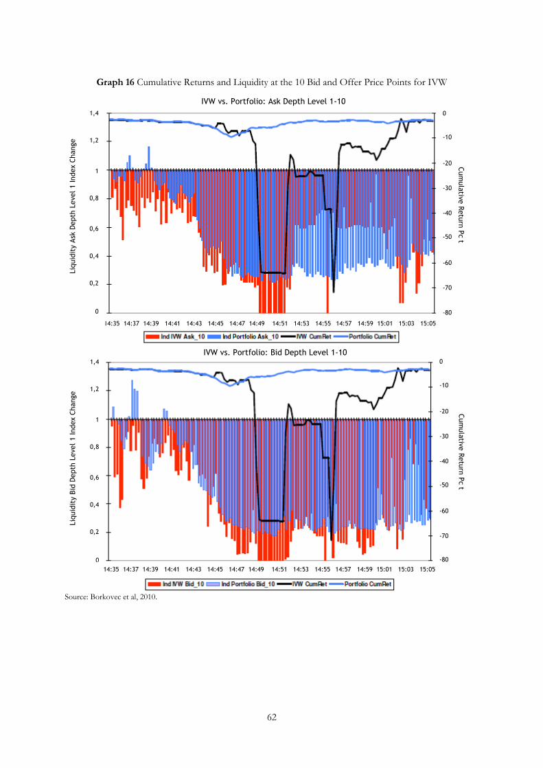
62

Graph 16 Cumulative Returns and Liquidity at the 10 Bid and Offer Price Points for IVW


14:35 14:37 14:39 14:41 14:43 14:45 14:47 14:49 14:51 14:53 14:55 14:57 14:59 15:01 15:03 15:05

IVW vs. Portfolio: Ask Depth Level 1-10

1,4

1,2

1

0,8

0,6

0,4

0,2

0

Liq

uid

ity A

sk D

epth

Level 1 Index C

hange

0

-10

-20

-30

-40

-50

-60

-70

-80

Cum

ula

tive R

etu

rn P

c t

IVW vs. Portfolio: Bid Depth Level 1-10

1,4

1,2

1

0,8

0,6

0,4

0,2

0

14:35 14:37 14:39 14:41 14:43 14:45 14:47 14:49 14:51 14:53 14:55 14:57 14:59 15:01 15:03 15:05

Liq

uid

ity B

id D

epth

Level 1 Index C

hange

0

-10

-20

-30

-40

-50

-60

-70

-80

Cum

ula

tive R

etu

rn P

c t

63


14:35 14:37 14:39 14:41 14:43 14:45 14:47 14:49 14:51 14:53 14:55 14:57 14:59 15:01 15:03 15:05

Graph 17 Cumulative Returns and Liquidity at the 10 Bid and Offer Price Points for SPY

SPY vs. Portfolio: Ask Depth Level 1-10

SPY vs. Portfolio: Bid Depth Level 1-10

14:35 14:37 14:39 14:41 14:43 14:45 14:47 14:49 14:51 14:53 14:55 14:57 14:59 15:01 15:03 15:05

1,6

1,4

1,2

1

0,8

0,6

0,4

0,2

0

1,4

1,2

1

0,8

0,6

0,4

0,2

0

0

-1

-2

-3

-4

-5

-6

-7

-8

-9

-10

0

-1

-2

-3

-4

-5

-6

-7

-8

-9

-10

Liq

uid

ity A

sk D

epth

Level 1 Index C

hange

Liq

uid

ity B

id D

epth

Level 1 Index C

hange

Cum

ula

tive R

etu

rn P

c t

Cum

ula

tive R

etu

rn P

c t

64

ETFs have been one the most affected categories during the Flash Crash as reported by the SEC,

who believes one of the main reasons for this disproportionate price volatility has been the draining

of liquidity as market makers decided to exit the market.

Together with their prices steep decline, the funds values started to deviate from their fundamental

price assuming different behaviors than their underlying portfolios. In those 20 minutes crash, their

price discovery mechanisms failed to take place and evidences about the existing relationship

between lack of liquidity and ETFs price discrepancies have been reported.

3. THE 2010 ENTAIL

After the 2010 Flash Crash, authorities decided to introduce some changes to the exchanges

regulations since the measures in place at that time proved not to be sufficient to prevent steep

prices declines. New guidelines for breaking “clearly erroneous trades” have been settled and

single-stocks trading halts introduced when securities prices are observed to be lower or higher

than the 10% of the previous 5-minutes trades prices. Furthermore, in 2013 the Limit Up Limit

Down (LULD) provision was implemented at the initiative of FINRA and the U.S. Exchanges in

order to give investors the possibility to revert sharp price movements before the trading activity

is stopped.

The aim of this system is to avoid the execution of trades above or below a certain range, computed

based on a security prevailing price, trading volume and time during the day. When a too high bid

price or a too low ask price are submitted in the trading book orders, the instrument in question

enters in a “Limit State” lasting 15 seconds. In this time frame, where the security trading keeps

going on, market participants have the possibility of reverting the price swing making the asset

exit this phase; if this does not happen though, trading activity is halted for 5 minutes. After the

pause, the exchange starts a re-opening auction where a new security price and bands are

determined in order to allow the trading to start again95.

Unfortunately, these reforms demonstrated to be still not enough to avoid flash crisis and the

propagation of noise throughout the markets. In fact, the Flash Crash of August 24, 2015 was the

first time where markets had the possibility of testing these changes that seemed to fit during

95 Jane Street Group, 2017.

65

standard trading activity. One of the main problems connected with the LULD trading halts was

in fact that they have been conceived for single-stock events and not for broad-market crisis.

The shock was mainly focused on the U.S. equities listed on the NYSE and related products, seeing

the S&P 500 sinking 5% and similarly to 2010, ETFs experiencing detachment from their

underlying portfolios.

We will now continue our analysis questioning why the new regulations weren’t sufficient to stop

this sharp decline and if common trends, between the two flash crashes, can be detected in ETFs

trading activity and related arbitrage mechanism.

On that day, investors were already filled with bearish sentiment from the previous week strong

selling pressures. Moreover, the Chinese Shangai Composite Index, which starts trading before the

U.S. market opening, was experiencing an 8,5% decline that, together with the widespread concerns

about China’s slowing economy, triggered volatility and sell-off globally. Indeed, global stocks

quotation were already down about 3%-5% and selling orders on the E-Mini were hitting during

the pre-opening market trading.

Given all these factors and the consequent volatility spreading, the NYSE decided to appeal to

Rule 4896 in order to quicken market openings in which it was a turbulent morning. The rule didn’t

require the quotation of a security neither to be announced nor to be endorsed by the stock market

managers before the markets opening. If on one hand this should cut-off some activities that

obviously require time, on the other it restrained the pre-opening information flow, fading price

transparency in a critical moment. Despite the implementation of this ruling, the stock exchange

experienced delays and almost the 50% of the listed stocks hadn’t yet began normal trading at 9:40.

The lack of proper information and the time-gaps in many securities openings enhanced

uncertainty in the stock market. holding back market makers to carry out their usual activity.

Securities started to show big price divergences even though in the same sector and the price of

some exchange traded products started to completely detach from their portfolios since arbitrage

activity failed to take place97.

Due to the heavy price swings and market imbalance at the opening, roughly 1.300 LULD trading

breaks took place from 9:30 to 10:30 of that morning. It’s worth to highlight that, if these pauses

96 The Rule was abolished in 2016. 97 BlackRock, 2015.

66

served as dampers for prices negative spikes, at the same time they slowed down prices recovery

as the rule applied to both lower and upper bands. As we said, this caused further and subsequent

halts, yet undermining price discovery and transparency, therefore. ETFs and ETPs in general

represented one of the most affected categories: of the total number of trading halts, 1000 of them

concerned ETPs.

LULD policies are not harmonized among the different stock exchanges and what played an

important role in the creation of this loop were also the rules settled by the NYSE Arca; it

represents the biggest U.S. ETFs exchange and the primary listing for more than the three-quarter

of U.S. ETPs. Indeed, this exchange provides predefined auction collars in order to avoid securities

opening or after-halt opening market prices to exceed a certain range. Problems arises when, due

to these constraints, during periods of noisy markets and several trading imbalances, market orders

are left unpaired and sent directly to the order books as soon as trading re-starts. On August 24 in

particular, unfulfilled ETPs selling orders directly reversed on the order books led to greater

volatility and further consequent LULD breaks.

Similarly to what happened during the 2010 Flash Crash, a broad number of ETFs experiences

significant prices discrepancies with respect to their portfolios due to the absence of their

underlying arbitrage activity. Indeed, arbitrageurs need proper market conditions to come into play

as arbitrage is never riskless and they need some sort of “warranty” when entering the game.

First, they must be able to properly evaluate the ETPs shares with respect to their portfolios prices

in order to understand if it does exist an arbitrage opportunity; this of course requires the

underlying value to be available and certain intraday. After it’s determined that arbitrage might be

advantageous, market conditions need to allow for the possibility to hedge the arbitrage trading

risk market participants are going to bear by taking a position on the ETPs i.e. markets need to be

liquid. Arbitrageurs will unlikely participate if unable to protect their trades. Finally, they need to

have the assurance their orders will be executed98.

That morning all these requirements were missing since several assets quotations weren’t available,

causing troubles on properly judging the ETPs values tracking them, LULD halts were limiting

disposable liquidity and the evaluation criteria regarding the clearly erroneous trades weren’t

straightforward. As a consequence, the arbitrage mechanism that usually keeps the ETFs prices

98 BlackRock, 2015.

67

and their NAV aligned failed to take place for a broad number of securities and, as we anticipated

several price discrepancies were observed.

The volume traded on this day spiked to one of the highest in U.S. equity and 37% of this were

represented by ETPs shares99.

The evidences brought out by the two flash crashes demonstrate that the arbitrage activity

underlying ETFs and ETPs in general is not always effective in maintaining their market price and

fundamental value aligned. Periods of high volatility and liquidity shortages have the potential to

be disruptive for investors and the broad market, creating big inefficiencies.

In both shocks, large order imbalances, trading halts and broken trades enhanced the noise already

spread in the exchanges and created further liquidity withdrawals, restraining the arbitrage activity

and consequently the price discovery potential of these funds. Indeed, ETFs based on more liquid

assets as large capitalization U.S. stocks, or the ones tracking unaffected securities as either bonds

or international shares, which didn’t experience any trading pause, maintained consistent prices

with their underlying portfolios.

Among all the characteristics that make ETFs so popular and that we described in the first chapter,

their greater liquidity in comparison with their underlying is surely one of the most appreciated by

investors. This latter, together with market transparency is a necessary part of their tracking

process. During the market history, as we reported in the second chapter, ETFs proved more than

once their price discovery potential even when their components markets were closed; we need to

bear in mind though, that arbitrage activity represents a fundamental part of this process.

Given the growing size of the ETFs industry, their increasing popularity in portfolios construction

as diversification instruments due to their relevant characteristics and the influence they have on

their underling portfolios considering their intrinsic cross-market activity, regulators should focus

on creating more ad-hoc reforms for these instruments to ensure transparency, versatility and

liquidity not to be undermined under both normal and critical market conditions.

99 BlackRock, 2015.

69

IV. REGULATORY EVOLUTION AND MIFID II IMPACT

So far, we focused mostly on the US market of Exchange Traded Funds. The main reason for this

choice relies on the size of it. In fact, US ETFs represented the 71% of the total AUM of the global

industry as the end of 2017, in so far being the one having the highest and most meaningful amount

of data. Moreover, the researches we’ve been analyzing are mainly focused on the SPDR S&P 500

since the biggest and most traded ETF in the world.

In this chapter instead, we are going to focus on the regulation of this industry in Europe since the

latest developments and the recent implementation of the Markets in Financial Instruments

Directive II represent a potential game changer for both markets.

1. EUROPEAN REGULATORY LANDSCAPE

US and European ETFs markets have been growing at the same pace in the recent years,

performing an average 18% growth rate. Despite that, Europe still accounts only for the 16% of

the global industry as a reflection of the main characteristics of this market.

Under European regulation, ETFs should fall below the rules instituted by the MiFID, being

securities traded on the stock exchange. However, MiFID I was introduced in 2007, dealing with

the guidance for credit institutions and investment firms providing financial services and for the

market operations performed by market participants, it wasn’t comprising ETFs as regulated

instruments; consequently, there was no need for these funds to follow its legal requirements as,

for example, the disclosure of the trading volume. The introduction of the MiFID II in 2018 was

aimed to fix this discrepancy and later in this chapter we are going to focus on that100.

The Undertaking for Collective Investment in Transferable Securities Directive gives the guidelines

for ETFs activity, providing three important principles. First of all, as to preserve diversification,

the holdings in the ETF portfolio cannot account for more than the 20% of the fund NAV each;

secondly, supervised by an external custodian bank, the ETF and its provider need to separate their

capital; finally, liquidity needs to be assured to the investor so that ETFs have to be open-ended

and redemption has to be possible anytime. The UCITS authorization is a globally recognized

guarantee that the fund is adopting high transparency and investors protection standards.

100 Thomadakis, 2018.

70

In 2012, the European Securities and Markets Authority carried out the first initiative specifically

directed to regulate ETFs, reinforcing their regulatory background and now requiring the disclosure

of the ETFs portfolio transparency policy and secondary market investors risks in the fund

prospectus. As an example, UCITS ETFs are required to display when and how the redemption of

their shares is possible to be carried out directly with the fund and the eventual costs involved; this

is usually allowed to secondary market traders only when big inefficiencies in the market appear

and the absence of market makers cause the ETF market price to strongly differ from the NAV.

As anticipated before, the lag of the European ETFs market with respect to the United States, is

due to some inner characteristics that have been observed developing over time. The fragmentation

of ETFs in Europe around different stock exchanges, has been contributing to the slower

development of the industry since too many funds are listed in an excessively high number of stock

exchanges: although the 85% of the European ETF turnover is generated by 3 main markets (LSE,

Euronext Paris and Euronext Paris, LSE and Deutsche Börse), 2.324 funds are scattered in 23

different exchanges while, the 2.173 U.S. ETFs are concentrated in only 3 stock exchanges.

Moreover, risk aversion and flexible pension plan systems are undermining the retail participation

to the investment funds industry in general and, in particular, to the ETFs world: only the 10% of

the European household financial assets is focused on collective investment schemes (22% in

U.S.)101.

Given that, retail investors attention is obviously more focused on instruments able to give a good

competitive advantage in a transparent manner. As a consequence of the failure of ETFs

classification as an asset class under MiFID I, and consequently no-obligation to report all the

trading activity executed on them, led to the development of ETFs bilateral transactions rather

than on-exchange trading. Over-the-counter ETFs trades are estimated to account for the 70% of

the total industry, failing to provide to investors the transparency level they ask for102.

Furthermore, exchange traded ETFs are still mostly used by institutional investors, as emerge by

looking at the distribution of the EU exchanges transactions. In fact, the size of an average

electronic order book transaction is way smaller than the ones occurring in negotiated deals. The

main difference between those two types of transactions is that while the former are exposed to all

market users and automatically executed within the rules set up by the exchange (minimum size as

101 The biggest part of households’ financial assets is focused for the 35% on currencies and deposits, 32% in insurances and pension funds and 20% invested in equity. 102 Thomadakis, 2018.

71

an example), the latter consist in a common agreement between buyer and seller occurring in a

parallel platform (managed by the stock exchange), that checks the consistency both with the

exchange provisions and the EOB price.

On-exchange negotiated deals are mostly used by institutional investors in order to execute

portfolio rebalancing or liquidity orders because they can interact directly with the counterparty

avoiding commissions, in order to trade ETFs shares without any size constraint. On the other

hand, EOB orders, being more regulated, benefit from greater transparency and are consequently

preferred by retail investors. In Europe, ETFs EOB are the 12% of the size of the average ND

transaction, while in U.S. the sizes are more similar, meaning that large retail and institutional

investors are the one dominating the on-exchange venues103.

2. MIFID II IMPLEMENTATION AND EFFECT ON EUROPEAN ETFS INDUSTRY

The recent introduction of MiFID II aims to bring more transparency on the European exchanges,

focusing on equity and some equity-based instruments, including ETFs. The new combination of

integrated rules aims to grant soundness and responsibility in more transparent financial markets,

to take steps forward against unregulated financial systems, as a G20 commitment, to bring greater

organization and transparency on OTC and commodities derivatives markets, to follow up

financial innovations such HFT (High Frequency Trading), algorithmic and dark trading and to

lower the member states discretion on financial markets regulation104.

It’s now possible to have a more consistent big picture of the trading volume of these instruments

across Europe. The new reporting obligations require all the trades, both on and off exchange, to

be reported and to be included in the consolidated tape105. Investors are now able to have a greater

consciousness on the true liquidity of the ETFs market in Europe, considering that European stock

exchanges sum up to 25 and ETFs can happen to be cross-quoted in multiple of them, showing

different prices. Euronext estimated that in 2018 the ETFs visible exchanged volume grew from

1,3$ trillion to 2,3$ trillion106.

103 Thomadakis, 2018. 104 Gomber et al, 2018. 105 It’s an electronic platform providing real time information on exchange traded securities volumes and prices. 106Bannon and MacManus, 2017.

72

MiFID II, providing also pre and post-trade transparency requirements, it’s enhancing the

investors’ confidence in the ETFs industry as an efficient and liquid market. Moreover, the new

imposition addressed to all the liquidity providers to register themselves as market makers has led

to a 25% increase of this actors in Europe. Their networking is growing, creating a more efficient

market: as we have seen, they are a fundamental part of the ETFs activity and greater is their

presence inside the ETF industry, simpler will be to trade these instruments, i.e. greater liquidity107.

As consequence of the greater transparency in the ETFs market, some authors sustain that these

funds will be increasingly used in security lending activities from investors up to increase their

revenues by taking more risk in their investments.

In addition, securities lending activities have been employing non-cash instruments as collateral

more often in the past years, comprising ETFs; in Europe though, this usage has been limited by

a common perception of poor liquidity. Because of the greater transparency in the European ETFs

market and its real trading volumes finally coming into light, some authors sustain that banks,

hedge funds and other institutional investors, will increasingly recognize these funds shares as a

guarantee in Europe as well108.

As we explained in the first chapter, the new regulation requires higher disclosure to funds, bank

and financial advisors on the fees and retrocessions they ask to their clients. This is creating more

awareness on the costs investors need to face and it’s fastening the shift of the wealth management

industry to a fee-based advisory model. Fee-based advisors are paid directly by the clients, usually

based on the AUM, and they need to act respecting fiduciary obligations. This shift can further

prompt the use of ETFs by advisors, as cost-efficient investment tools, perfectly suitable to build

diversified portfolios109.

Accordingly to all that has been said, the introduction of this new regulation is expected to boost

the attractiveness of ETFs in Europe, both for retail and institutional investors. Even though not

so much time has passed since the MiFID II implementation, ETFs providers have already started

seeing some positive effect: in June 2018, the Head of BlackRock iShares EMEA Stephen Cohen,

stated that, from only 6 months since the implementation of the regulation, the full range of iShares

107Chandler, 2018. 108 Rust, 2018. 109 Chandler, 2018.

73

UCITS ETFs has been experiencing a 61% increase in the trading activity and 74% for Fixed

Income ETFs.

As we said, the new requirements imposed starting from January 2018, do not concern exclusively

the disclosure of trading volumes. To ensure transparency both in the pre and post trading phase,

market makers are required to disclose bid-ask spreads and details regarding each transaction done.

However, MiFID II also involves the use of “waivers”, in order to delay the publication of prices

when large-volume trades or orders on less traded instruments are likely to heavily affect the price

of the traded security. Besides the European Securities and Markets Authority defined the rules to

compute such waivers for all the equity and equity-like financial instruments, they are claimed to

be not suitable for ETFs. The main concern of market makers is that, due to inappropriate

threshold they are not going to be able to use them in the right moment, causing large price

fluctuation in ETFs prices.

In the last chapter we have found evidences on how ETFs trend are able to move the market of

their underlying assets and how they create the base for common movements in their returns.

Consequently, if big price fluctuations are not prevented to happen, they have the potential to

spread all over financial markets, causing noise for non-fundamental reason. In addition, this risk

might cause a loss of interest by investors more focused on price stability rather than higher returns.

For example, many pension funds may decide to give up big volumes of ETFs shares, creating

more prices pressure and triggering a dominos effect.

This is the reason why, if on one hand MiFID II is pushing the ETFs industry growth, on the other

regulators need to closely follow-up its effect on the European market, ETFs in particular, given

the financial stability risks it can be subject to110.

The new developments in the European regulation might spread their effects overseas as well. Due

to the lack of clarity about the real liquidity of European ETFs, investors often chose to direct their

investments in comparatively more transparent jurisdiction i.e. U.S. market.

For example, aiming to shed more limpidity to the fees applied by asset managers, the new rules

introduced by MiFID II expect the research expenses to be now sold and payed separately from

trading expenses. This has caused a big change in the traditional market where banks and broker

have always sold market analysis and research together with trading services, like a unique package.

110 Bannon and MacManus, 2017.

74

Such development has the potential to lower trading costs, increase the quality of the researches

and let investors to be more aware of how their money are spent, shifting their attention closer to

the European market111.

With higher trading efficiency and more consistent liquidity recording, investors should gradually

lose the incentive to invest in overseas ETFs market, considering the advantage of European

trading hours as well112.

Moreover, the introduction of the KID requirement represents the most important growth

opportunity for the European ETFs market. In fact, retail European investors are now forbidden

from buying shares of a specific investment fund if the issuer is not providing the Key Information

Document, i.e. a key document about the fund investment objectives, risk and reward strategies,

applied fees and performance aimed to facilitate the potential client comparison of different

products.

Consequently, for those investors it’s now impossible to invest in the biggest and most popular

ETFs in the world as the SPY, the QQQ (the PowerShares QQQ Trust Series 1 ETF tracking the

Nasdaq 100) and the EEM (the iShares MSCI Emerging Markets ETF), that don’t have a KID;

they can either keep them or sell them if they already own some shares. Of course, the document

is not impossible to be provided by the U.S. funds issuers but it requires the disclosure of different

fund data as pricing information and time and since U.S. ETFs are not truly thought to be traded

by European retail clientele there might be low motivation in creating this document.

Considering the size of these ETFs and the width of their clientele, the effect of this restriction

won’t be strongly impactful but, on the other hand, this can benefit European ETFs by further

boosting the adoption of the region ETFs by non-professional investors113.

Europe already has alternatives which investors can buy in order to overtake this limit as the SPY5

(SPDR S&P 500 UCITS ETF) or the CSPX (the iShares Core S&P 500 UCITS ETF USD). In this

regard, the latter has hit a new record in 2018, becoming the biggest ETF domiciled in Europe

with 30$ billion AUM. BlackRock Head of iShares EMEA explains that, among other factors like

111 Bloomberg's Editorial Board, 2018. 112 McNeil, 2018. 113 Vannucci, 2018.

75

positive sentiments on U.S. stocks drove by strong earnings and growth, Also the introduction of

MiFID II has of course played an important role in boosting in the inflow towards the CSPX114.

Analysts estimate that European ETFs AUM have now the potential to grow up to 2$ trillion in a

5-years time115.

One of the main reasons why the ETFs market in Europe has lagged behind the volumes of U.S.

Exchange Traded Funds is because it has always comparatively lacked in transparency and

integration. This caused these instruments to be mostly employed by institutional investors in OTC

markets, wiping out an important part of the potential clientele, i.e. retail investors. Now that a new

set of comprehensive European rules has been introduced to enhance investors protection and

shade a light on this previously poorly regulated market, and that limits and improvements have

been made with respect to foreign markets, many professionals think this is going to positively

impact the ETFs industry of the continent.

So far, only one year has passed since the introduction of MiFID II and thorough analysis of the

effect have still to be carried out; the biggest ETFs sponsor though, they have already begun to see

the positive effect of the new rulings and the increase of new market makers is helping to further

enhance the investors’ confidence in the liquidity and the depth of this market.

More time will be needed to see the overall and complete consequences on European capital

markets.

114 Lord, 2018. 115 Vannucci, 2018.

77

V. CONCLUSIONS

The financial industry has been subjected to several changes in the last years. Investors are shifting

their investment strategies, now favoring passive investing, pushed by increasing information

democratization, new regulatory frameworks, index proliferation, new automated investing

platforms and mediocre active funds after-fees performances.

Among all the available instruments, ETFs have been the ones experiencing the greatest inflows

and this comes with no surprise considering their intrinsic characteristics. These funds, besides

their low fees and cost efficiency, they usually benefit from higher liquidity with respect to the

securities they are tracking and from a good level of transparency since they need to disclose the

components of their portfolios daily, opposed to other types of investment funds. They give to

investors new opportunities of diversification by tacking positions in markets unavailable before

and representing perfect building blocks for portfolio construction.

Their increasing popularity, in conjunction with their shares creation and redemption mechanism

and intrinsic arbitrage activity, are giving some cause for concern though as potential threats to the

stability of financial markets.

ETFs create two different trading levels, a primary venue involving transactions between the

provider and the APs and a secondary between the APs and the global exchanges. This adds a

further liquidity layer to the ETFs underlying assets that can result in two different consequences:

when mispricing appears (conceived as the difference between the ETF price and its NAV) it either

can be part of a price discovery process, enhancing information spreading, or it can propagate non-

fundamental shocks from the fund to the securities when shocks take place.

In the second chapter we focused on answering our questions relating the ETFs potential for non-

fundamental shocks spreading and underlying assets returns volatility.

Madhavan and Sobczyck demonstrated that during the 2008-2009 financial crisis, mispricing was

caused by staleness in the NAV meaning that ETFs, as more liquid instruments, did the first move

and the underlying assets followed. Similarly, during the Egyptian market closing for the Arab

Spring, ETFs based on its stocks kept trading, giving investors consisting expectations on the

further evolution of that market.

78

On the other hand, given that ETFs price dynamics are always driven by their intrinsic arbitrage

activity, as opposed to the latter view, other academics conducted several researches demonstrating

the existence of non-fundamental shocks transmission potential from the funds to their

components as arbitrageurs take opposite position on them. The concern that ETFs can actually

spread noise into their porfolios is even enhanced by the fact that in the recent years, ETFs have

been increasingly employed for hedging and speculative aims.

The results obtained by David, Franzoni and Moussawi’s study support this theory, showing that

arbitrage activity is not only helping to keep the ETFs prices and their NAV aligned but it can

represent a risk for financial markets since it has the potential to move the price of correctly-valued

securities and consequently causing noise transmission and volatility in the underlings included in

the ETF portfolio.

After finding evidences on the existence of a causal relationship between the ETFs ownership of

a stock and its return volatility, the consequent question has been to wonder if, transmitting the

same shock to all their portfolio, ETFs create commonality in their underlings returns behaviors.

Wurgler (2011) demonstrates that as a new stock is included in the S&P 500, its return pattern

starts to move more alike the other securities included in the index portfolio, mainly due to the

correlated money outflows and inflows the stocks experience after their inclusion Given that

arbitrage activity has a stronger potential, with respect to correlated money flows, to drive returns

commovement, in 2017 Da and Shive investigated on the existence of this latter link between ETFs

portfolios inclusion and increasing similarity in the components returns behavior.

From their study it emerges that ETFs turnover, used as a proxy of ETFs arbitrage activity,

represents a driver of correlation among stocks returns being itself correlated with stocks turnover

throughout arbitrage activity. Bearing in mind that arbitrage is advantageous only when the

securities involved can be easily and not expensively traded, as a further evidence favoring their

theory, the two authors finds out that arbitrage activity has a greater influence on the correlation

of the underlying assets returns for all the ETFs having their baskets made by more than the

99,67% of stocks.

Since ETFs can employ different approaches in order to track their underlings, we also asked if

and in which way this can create threats to financial market stability. Indeed, the last part of the

second chapter is focused on the risk represented by synthetic replication methods, as opposed to

the effect that physical ETFs activity has on the funds underlying assets. While the investors on

79

the latter category are exposed to a tracking error risk, synthetic ETFs are exposed to a counterparty

risk. Investors common perception of ETFs market as liquid can lead them to underestimate the

market risk deriving from the increasing complexity of these products, also considering that when

employing synthetic replication approaches, products transparency decreases since different players

and markets come into play and risk monitoring ability decreases.

Relating to the two latter questions leading this work, in the third chapter we found evidences on

the importance of market makers and institutional investors activity in maintaining ETFs efficiency,

particularly with regards to the alignment between funds shares prices and their NAV.

In fact, different events in the recent history have demonstrated that ETFs can represent a risk for

systemic financial stability, especially during time of market stress where liquidity shortages and

limits to arbitrage activity starts to appear. During the Flash Crash happened in May 2010 for

example, the S&P 500 sank roughly the 9% in 20 minutes, probably caused by the spreading of the

unusual volatility. During this crash, ETFs have been the one category hit the most by the shock

showing steep decline in prices and strong detachment from their underlings values. On this

occasion, similarly to what happened in 2015 besides the new reforms taken by regulators, arbitrage

activity failed to take place: due to poor liquidity, high volatility, prices uncertainty and low

transparency, many market makers and other participants exited the market stopping to perform

arbitrage activity.

The ETFs industry is growing, their popularity as diversification blocks in portfolios construction

is increasing and given their influence on their underling assets due to their intrinsic cross-market

activity and the reliance investors have on their liquidity, regulators should focus on the

preservation of ETFs transparency, versatility and liquidity under both normal and critical market

conditions.

The recent implementation of MiFID II in Europe has the objective to shade a light on this sector.

Increased regulation, greater disclosure and a higher number of market makers is helping to further

enhance the investors’ confidence in the liquidity and depth of this market and even though only

one year has passed by, ETFs sponsor have already started to see positive effect in the sector

inflows.

ETFs are one of the most innovative financial instruments. They give investors new opportunities

for diversification and can be elements of price discovery at times. Their virtues come with some

flaws and risk though, mostly related to their intrinsic mechanics. Regulations and reforms can

80

provide a protection against the inefficiencies these instruments can bring to the market and their

potential for noise spreading but the underlying risk represented by liquidity shortages and arbitrage

activity failure will be hard to defeat. For this reason, investors should be cautious and perfectly

aware of this industry characteristics.

81

BIBLIOGRAPHY

Amihud Y., and Mendelson H. (1986), "Asset Pricing and the Bid-Ask Spread", Journal of Financial

Economics, Vol. 17, pp. 223–249;

Anadu K., Kruttli M., McCabe P., Osambela E. and Shin C. (2018), The Shift from Active to Passive

Investing: Potential Risks to Financial Stability? , Federal Reserve Bank of Boston, Working Paper No.

RA 18-04;

Bannon D. and MacManus C. (2017), ETF market in Europe, Deloitte;

Ben-David I., Franzoni F. and Moussawi R. (2012), ETFs, Arbitrage, and Shock Propagation; National

Centre of Competence in Research Financial Valuation and Risk Management, Working Paper N

793;

Ben-David I., Franzoni F. and Moussawi R. (2015), Do ETFs Increase Volatility?; Charles A. Dice

Center for Research in Financial Economics, Working Paper;

Ben-David I., Franzoni F. and Moussawi R. (2017), Exchange Traded Funds (ETFs), Charles A. Dice

Center for Research in Financial Economics, Working Paper;

Bloomberg's Editorial Board (2018), Europe’s MiFID II Challenge to U.S. Finance, Bloomberg,

02/01/201;

BlackRock (2015), US Equity Market Structure: Lessons From August 24, Viewpoint October 2015;

Borkovec M., Domowitz I., Serbin V. and Yegerman H. (2010), Liquidity and Price Discovery in

Exchange-Traded Funds: One of Several Possible Lessons from the Flash Crash, ITG;

Busse J., Goyal A. and Wahal S. (2014), "Investing in a Global World", Review of Finance, 2014, 18,

pp. 561–590;

Carhat M. (1997), "On Persistence in Mutual Fund Performance", The Journal of Finance, Vol. 42, 1,

pp. 57-82;

Chandler B. (2018), "iShares’ Cohen comments on first six months of MiFID II’s effect on ETFs"; ETF

Express, 11/07/2018;

Cremers M., Ferreira M., Matos P. and Starks L. (2016), "Indexing and active fund management:

International evidence", Journal of Financial Economics, 120, pp. 539–560;

Da Z. and Shive S. (2017), Exchange traded funds and asset return correlations, Wiley European Financial

Management;

Evans R. and Wilson C. (2018), How ETFs became the market, Bloomberg, 13/09/2018;

EY (2017), Reshaping around the investor, Global ETF Research 2017;

Fama E. and French K. (2010), "Luck versus Skill in the Cross-Section of Mutual Fund Returns",

The Journal of Finance, Vol. 65, 5, pp. 1915-1947;

82

Fama E., Fisher L., Jensen M. and Roll R. (1969), “The Adjustment of Stock Prices to New

Information”, International Economic Review, Vol. 10;

FTSE Russell (2017), The Growth of Passive Investing: Has There Been an Impact on the US Equity Market?,

Research September 2017;

Gomber P., Clapham B., Lausen J. And Panz S. (2018), The Impact of MiFID II / MiFIR on European

Market Structure - A Survey among Market Experts -, Goethe University Frankfurt;

Hill J., Nadig D. and Hougan M. (2015), A Comprehensive Guide to Exchange Traded Funds, The CFA

Institute Reseach Foundation;

Jane Street Group (2017), Market Structure and ETF Strategy, 04/04/2017;

Janson M. (1968), "The Performance of Mutual Funds in The Period 1945-1964", The Journal of

Finance, Vol. 23, 2, pp. 389-416;

Lettau M. and Madhavan A. (2017), "Exchange-Traded Funds 101 for Economists", Journal of

Economic Perspective, Vol.32, 1, PP, 135-154;

Li F. and Zhu Q. (2016), Synthetic Shorting with ETFs;

Lord J. (2018), BlackRock’s iShares Core S&P 500 UCITS ETF crosses $30bn milestone, ETF Strategy,

01/08/2018;

Malamud S. (2015), A Dynamic Equilibrium Model of ETFs;

McNeil H. (2018), Why MiFID II takes away US edge in ETFs, Investment Week, 11/04/2018;

Mhadavan A. and Sobczyk A. (2015), Price Dynamics and Liquidity of Exchange-Traded Funds,

BlackRock;

Morck R. and Yang F. (2001), The Mysterious Growing Value of S&P Index Membership, NBER,

Working Paper No. 8654;

Ramaswamy S. (2011), Market Structures and Systemic Risks of Exchange Traded Funds, BIS, Working

Paper No. 343;

Rust S. (2018), MiFID II to spur greater ETF usage in securities lending, IPE, 04/01/2018;

SEC (2009), Leveraged and Inverse ETFs: Specialized Products with Extra Risks for Buy-and-Hold Investors,

01/08/2009;

SEC and CFTC (2010), Findings Regarding the Market Events of May 6, 2010, 30/09/2010;

SEC and CFTC (2010), Preliminary Findings Regarding the Market Events of May 6, 2010, 18/05/2010;

Small M., Cohen S. and Dieterich C. (2018), Four big trends to drive ETF growth, BlackRock;

Stambaugh R. (2014), "Investment Noise and Trends", The Journal of Finance, Vol. 69, 4, pp. 1415–

1453;

Sushko V. and Turner G. (2018), "The implications of passive investing for securities market",

BIS Quarterly Review, March 2018, pp. 113-131;

83

Thorpe D. (2018), Mifid II to Slash managers' fees by 10 to 15%, FT Financial Adviser, 15/01/2018;

Thomadakis A. (2018), The European ETF Market: What can be done better?, European Capital Markets

Institute, Commentary No. 53;

Ullal A. (2018), Sizing the "Smart Beta" ETF Market Globally, Wealth Management, 08/05/2018;

Vannucci C. (2018), European Investors Are Now Blocked From Investing in One of the Most Popular ETFs,

Bloomberg, 23/02/2018;

Wurgler J. (2011), "On the Economic Consequences of Index-Linked Investing", in Rosenfeld G.,

Lorsch J., and Khurana R. (edited by), Challenges to Business in the Twenty-First Century, American

Academy of Arts and Sciences, pp, 20-34.

84

SITIOGRAPHY

https://www.etf.com/etf-education-center/21038-how-to-run-an-index-fund-full-replication-vs-

optimization.html?nopaging=1;

http://www.etfwatch.com.au/blog/the-etfs-with-the-highest-inflows-in-fy-2018;

https://www.ftadviser.com/david-thorpe;

https://us.spdrs.com/etf/spdr-sp-500-etf-SPY.

http://www.etfwatch.com.au/blog/the-etfs-with-the-highest-inflows-in-fy-2018

https://us.spdrs.com/etf/spdr-sp-500-etf-SPY

ETFs: Investigation on the Possible Threats to Financial ...

Documents

Transcript of ETFs: Investigation on the Possible Threats to Financial ...