Estimation of DOAs of Acoustic Sources in the Presence of...

Estimation of DOAs of Acoustic Sources in

the Presence of Sensor with Uncertainties

Anurag Patra

Roll No: 212EC6193

Department of Electronics & Communication Engineering

National Institute of Technology, Rourkela

Odisha- 769008, India

Estimation of DOAs of Acoustic Sources in

the Presence of Sensors with Uncertainties

A Thesis Submitted in Partial Fulfilment

of the Requirements for the Award of the Degree of

Master of Technology

In

Electronics and Communication Engineering

By

Anurag Patra

Roll No: 212EC6193

Under the supervision of

Prof Lakshi Prosad Roy



Odisha- 769008, India

Declaration

I hereby declare that

1) The work presented in this paper is original and has been done by myself under the

guidance of my supervisor.

2) The work has not been submitted to any other Institute for any degree or diploma.

3) The data used in this work is taken from only free sources and its credit has been cited

in references.

4) The materials (data, theoretical analysis, and text) used for this work has been given

credit by citing them in the text of the thesis and their details in the references.

5) I have followed the thesis guidelines provided by the Institute.

Anurag Patra

30th

may 2014



CERTIFICATE

This is to certify that the Thesis Report entitled “Estimation of DOAs of Acoustic

Sources in the Presence of Sensors with Uncertainties” submitted by ANURAG PATRA

bearing roll no. 212EC6193 in partial fulfilment of the requirements for the award of Master

of Technology in Electronics and Communication Engineering with specialization in “Signal

and Image Processing” during session 2011-2013 at National Institute of Technology,

Rourkela is an authentic work carried out by him under my supervision and guidance.

To the best of my knowledge, the matter embodied in the thesis has not been submitted

to any other University / Institute for the award of any Degree or Diploma.

Prof. Lakshi Prosad Roy

Assistant Professor

Date: Department

of ECE

National Institute of Technology

Rourkela-769008

ACKNOWLEDGEMENTS

First of all, I would like to express my deep sense of respect and gratitude towards my

advisor and guide Prof. L.P.ROY, who has been the guiding force behind this work. I am

greatly indebted to him for his constant encouragement, invaluable advice and for propelling

me further in every aspect of my academic life. His presence and optimism have provided an

invaluable influence on my career and outlook for the future. I consider it my good fortune to

have got an opportunity to work with such a wonderful person.

Next, I want to express my respects to Prof Samit Ari, Prof. S. K. Patra, Prof. K. K.

Mahapatra, Prof. S. Meher, Prof. S. K. Das,Prof S. Maiti, Prof. Poonam Singh and Prof.

A.K.Sahoo for teaching me and also helping me how to learn. They have been great sources

of inspiration to me and I thank them from the bottom of my heart.

I also extend my thanks to all faculty members and staff of the Department of

Electronics and Communication Engineering, National Institute of Technology, Rourkela

who have encouraged me throughout the course of Master’s Degree.

I would like to thank all my friends and especially my classmates for all the thoughtful

and mind stimulating discussions we had, which prompted us to think beyond the obvious. I

have enjoyed their companionship so much during my stay at NIT, Rourkela.

I am especially indebted to my parents for their love, sacrifice, and support. They are

my first teachers after I came to this world and have set great examples for me about how to

live, study, and work.

Anurag Patra

Roll number: 212EC6193

Date: Dept. of ECE

National Institute of Technology

Rourkela

i

Abstract

Direction of Arrival (DOA) estimation finds its practical importance in sophisticated

video conferencing by audio visual means, locating underwater bodies, removing unwanted

interferences from desired signals etc. Some efficient algorithms for DOA estimation are

already developed by the researchers . The performance of these algorithms is limited by the

fact that the receiving antenna array is affected by some uncertainties like mutual coupling,

antenna gain and phase error etc. So considerable attention is there in recent research on this

area.

In this research work the effect of mutual coupling and the effect of antenna gain and

phase error in uniform linear array (ULA) on the direction finding of acoustic sources is

studied. Also this effect for different source spacing is compared. For that, estimates of the

directions of arrival of all uncorrelated acoustic signals in the presence of unknown mutual

coupling has been found using conventional Estimation of Signal Parameters via Rotational

Invariance Technique (ESPRIT). Also DOAs are computed after knowing the coupling

coefficients so that we can compare the two results. Simulation results have shown the fact

that the degradation in performance of the algorithm due to mutual coupling becomes more if

the sources become closer to each other. Also we have estimated DOAs in the presence of

unknown sensor gain and phase errors and we have compared this results with the results we

got by considering ideal array. Finally in this case also the effect of gain and phase error as

the source spacing varies has been tested. Simulation results verify that performance

degradation is more if the sources become closer.

Keywords: gain error, phase error, ESPRIT algorithm, mutual coupling, acoustic signal

uniform linear array (ULA), source spacing

ii

TABLE OF CONTENTS

Abstract………………………………………………………………i

Table of Contents…………………………………………………....ii

List of figures………………………………………………………..iv

Abbreviations………………………………………………………..v

Chapter 1 Introduction

1.1 Motivation………………………………………………………………..1

1.2 Objective…………………………………………………………………2

1.3 Outline……………………………………………………………………3

Chapter 2 Fundamentals of DOA estimation

2.1 Basic Theory of Antenna Array……………………………………......4

2.1.1 Two element antenna array……………….………………….........5

2.1.2 Steering matrix………………………………………………….....9

2.1.3 Uncertainties in antenna array ……………………………….......10

2.2 Basic Principles of DOA estimation………………………………......11

2.2.1 DOA estimation by Correlation Method……………………........15

2.2.2 DOA estimation by Maximum Likelihood Method……………...16

2.2.3 DOA estimation by MUSIC……………………………………...17

2.2.4 DOA estimation by ESPRIT……………………………………..21

Chapter 3 Literature Review…………………………………………..24

iii

Chapter 4 Effect of mutual coupling on DOA estimation

4.1 Formation of coupling matrix for DOA estimation………………….29

4.2 DOA estimation based on ESPRIT algorithm……………………....32

4.3 Simulation Results……………………………………………….......34

Chapter 5 Effect of antenna gain and phase error on DOA

Estimation

5.1 Modification of steering matrix in presence of antenna gain and phase

error…………………. ……………………………………………....38

5.2 DOA estimation using non-ideal steering matrix………………….....40

5.3 Simulation results…………………………………………………….42

Chapter 6 Conclusion

6.1 Conclusion…………………………………………………………..46

6.2 Future Work………………………………………………………….46

References…………………………………………………………………...47

Publication…………………………………………………………50

List of Figures

iv

2.1 Two element antenna array……………………………………………………………….6

2.2 Far field approximation of two element array……………………………………………7

2.3 Set up for steering vector determination………………………………………………….9

2.4 Set up for DOA estimation……………………………………………………………....14

4.1 Sketch map of mutual coupling for URA considering each sensor is affected by the

coupling from the 8 neibhouring sensors……………………………………………………30

4.2 Sketch map of mutual coupling for ULA considering each sensor is only affected by two

nearest neighbour.…………………………………………………………………………….31

4.3 RMSE of the estimated directions versus SNR of the signals

coming from 10◦,30

◦,50

◦ ……………………………………………………………………...36



◦,30

◦ ……………………………………………………………………...36



◦,26

◦………………………………………………………………………37



◦,20

◦………………………………………………………………………37

5.1RMSE of the DOA estimates versus SNR of the signals


◦,44

◦………………………………………………………………………44

5.2 RMSE of the DOA estimates versus SNR of the signals


◦,40

◦………………………………………………………………………44



◦,36

◦………………………………………………………………………45



◦,30

◦………………………………………………………………………45

Abbreviations

v

DOA – Direction of Arrival

MUSIC - Multiple SIgnal Classification

ESPRIT- Estimation of SIgnal Parameters via Rotational Invariance

Technique

EVD - Eigen Value Decomposition

DSB - Delay and Sum beamformer

GCC - generalized cross correlation

MCM - Mutual Coupling Matrix

PHAT - Phase Transform

TDE - Time Delay Estimate

SV- Steering Vector

MLM - Maximum Likelihood Method

CRLB - Cramer Rao Lower Bound

SNR- Signal to Noise Ratio

RMSE - Root Mean Square Error

ULA –Uniform Linear Array

URA - Uniform Rectangular Array

TM – Toeplitz Matrix

AWGN – Additive White Gaussian Noise

1

Chapter 1

Introduction

1.1 Motivation

Direction of arrival (DOA) estimation for Speech or acoustic signals with

mouthpiece cluster has various applications now a days. Estimations of DOAs with the

assistance of mouthpiece might be utilized to direct cameras to the speaker in video

conferencing session or a long distance classroom [1]. The working of the camera might be

took care of in one of three routes in present video conferencing frameworks or long

separation feature classrooms,. Cameras that give distinctive settled perspectives of the room

might be put at diverse areas in the meeting room to cover all the individuals. Furthermore the

framework could comprise of one or two cameras worked through people. Finally the

framework could comprise of switches those are operated manually for every client or

gathering of clients that might control the camera toward them when actuated. Third class of

frameworks is utilized regularly within long separation training that uses TV based

classrooms. These frameworks end up being costly as far as additional equipment or labor

needed to work them successfully and dependably. It might be attractive to have a few

cameras that could be naturally controlled to turn to the speaker. Most gatherings and

classrooms commonly have one man talking at once and all others tuning in. The speaker,

also can move within the room. So it is needed to have a framework that successfully and

dependably spots and tracks a solitary speaker. Single speaker confinement and following

could be performed utilizing either visual or acoustic information. An exhaustive following

framework utilizing video data was created by Wren et al. [2]. However, the algorithmic

2

multifaceted nature and computational burden needed for such a framework infers, to the

point that a completely devoted workstation be devoted to performing this task. Methods

focused around acoustic information are commonly far easier as far as multifaceted nature and

computational burden.

Another requisition of DOA estimation utilizing mouthpiece is a part of speech

enhancement for human workstation interfaces that rely on upon speech inputs from human

being [3]. Techniques utilized here, in the same way as superdirective beamforming, rely on

upon faultless assessments of the DOA of the acoustic signals. The same is the situation in

portable hearing assistants that utilize versatile beamforming to catch acoustic signals in the

presence of noise.

In a radar framework DOA estimation is of incredible significance keeping in mind

the end goal to spot the signal landing from a potential target. Electronic guiding might

replace the mechanical directing for this situation of the radar antenna. Also in wireless

communication environment determination of the coveted client at the base station might

bring about minimizing the obstruction from different users. This may be carried out by

heading the principle beam of the antenna towards the wanted client or regulating nulls

towards the meddling clients.

1.2 Objective

The objective of this research is to study the effect of antenna array uncertainties like

mutual coupling and antenna gain and phase error on the high resolution direction finding

algorithms. Also effect of these uncertainties as the spacing between sources varies has been

shown.

3

1.3 Outline

This thesis is divided into the following chapters in order to explain the works done

and showing the results in a lucid manner.

Chapter 2 covers the basic antenna theory with a emphasis on sensor uncertainties

between elements of an antenna array. After that the basic subspace based popular DOA

estimation methods has been discussed.

Chapter 3 gives a glimpse of current research on this area by various scientists.

In Chapter 4 the modified ESPRIT algorithm in the presence of mutual coupling has

been given and degradation in performance as the sources becomes closer has been studied.

In Chapter 5 the modified ESPRIT algorithm in the scenario of unknown antenna gain

and phase errors has been given and the effect of these uncertainties on the estimation process

for different source spacing has been given.

Chapter 6 , the last chapter of this thesis gives the conclusion, summary of the work

done and some future scopes of this project.

4

Chapter 2

Fundamentals of DOA estimation

2.1 Basic theory of antenna array

The electric field variation with angle (θ,ϕ) (i.e radiation patterns) of solitary element

antennas are broad normally., means directivity (gain) is relatively less. In the scenario of

communication in long distance, radiators having high directivity are badly required. (This is

true for receiving antennas too. For them it is required that they can only receive a particular

signal from a particular direction to avoid picking up unwanted signal.) Such antennas are

feasible to form by increasing the area of the radiating slot (size larger than λ ). Multiple side

lobes can appear however by adopting this technique. Besides, the size of the antenna

becomes large and very problematic to manufacture. Another procedure to enhance the

electrical size of a radiator is to form it as an Array of radiating elements in a efficient

configuration –array antenna. Generally, the characteristics of array elements are same. But

this is not indispensable always but it is practical and easier for manufacturing. The

individual elements of the system may be of any shape like loops, wire dipoles, apertures, etc.

The total field of an array can be calculated by vector superposition of the fields

radiated by a single antenna.(For receiving array same logic can be applied). For very

directional pattern, it is must that the individual fields (emitted by the individuals) add up by

constructive interference occur in the desired direction and destructive interference happens

in the remaining space.

5

Five methods for shaping the beam pattern of antenna array:

a) the shape of the array (linear, rectangular, circular, spherical, etc.),

b) the position of the individuals with respesct to others,

c) the driving magnitude of individual elements,

d) the phase of the driving input of each member,

e) the radiation pattern of individuals

2.1.1 Two-elements antenna array

Let s give the electric fields in the far field of the antenna array in the following form

(2.1)

(2.2)

6

Fig 2.1: Two element antenna array

Here:

, : magnitudes of the electric fields(do not include the 1/r factor);

, : field patterns (normalized);

, : distances from the 1st and 2

nd element to the observation point P;

: difference in phase between the feed or excitation of the two array elements;

, : polarization vectors associated with the far-zone E fields.

7

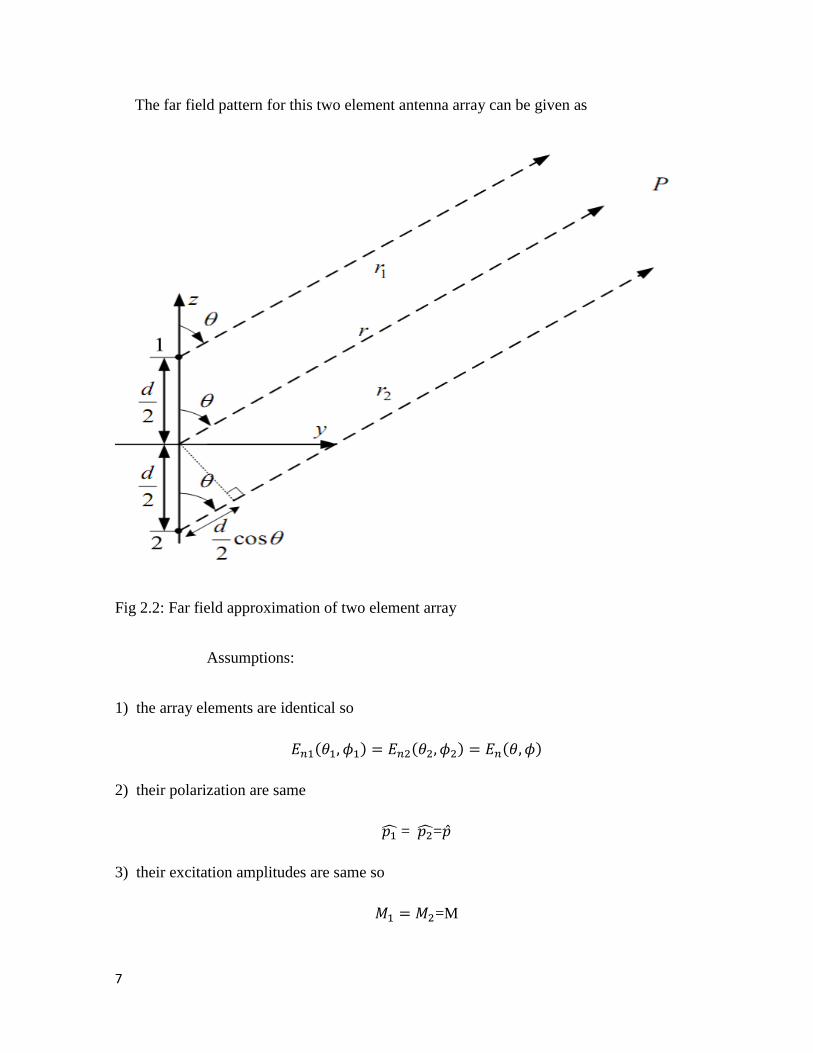
The far field pattern for this two element antenna array can be given as

Fig 2.2: Far field approximation of two element array

Assumptions:

1) the array elements are identical so

2) their polarization are same

= =

3) their excitation amplitudes are same so

=M

8

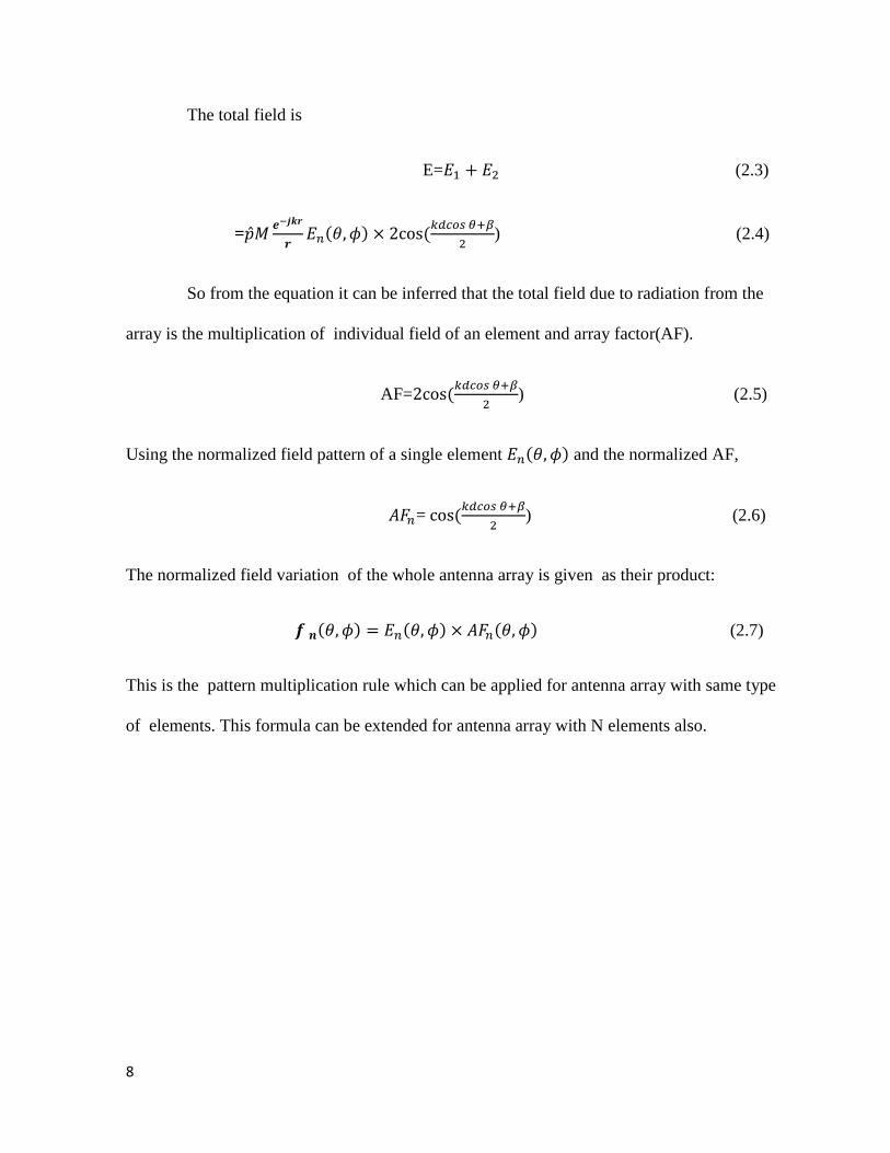
The total field is

E= (2.3)

=

) (2.4)

So from the equation it can be inferred that the total field due to radiation from the

array is the multiplication of individual field of an element and array factor(AF).

AF=

) (2.5)

Using the normalized field pattern of a single element and the normalized AF,

=

) (2.6)

The normalized field variation of the whole antenna array is given as their product:

(2.7)

This is the pattern multiplication rule which can be applied for antenna array with same type

of elements. This formula can be extended for antenna array with N elements also.

9

2.1.2 Steering matrix

Fig 2.3: Set up for steering vector determination

Suppose this is the sensor array. For far field approximation the delay time between

the first or leftmost individual and the next elements (2,3,4,5) are

Suppose the signal received by the 1st individual is So

(2.8)

In the same way

(2.9)

(2.10)

(2.11)

10

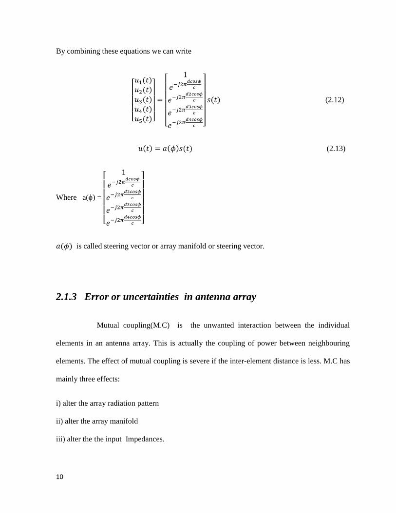
By combining these equations we can write

[ ]

[

]

(2.12)

(2.13)

Where a(ϕ) =

[

]

is called steering vector or array manifold or steering vector.

2.1.3 Error or uncertainties in antenna array

Mutual coupling(M.C) is the unwanted interaction between the individual

elements in an antenna array. This is actually the coupling of power between neighbouring

elements. The effect of mutual coupling is severe if the inter-element distance is less. M.C has

mainly three effects:

i) alter the array radiation pattern

ii) alter the array manifold

iii) alter the the input Impedances.

11

Eigen- structure based direction-estimating techniques such as MUSIC require

exact information about the signals received by the sensor array from a source located

at any angle. The performance of the eigenstructure based system depends strongly on the

accuracy of this steering matrix or array manifold. Calibrating an antenna array system

designed for two-dimensional (azimuth and elevation) direction finding with the precision

required by these superresolution techniques have various practical problems. There is the

problem of maintaining array Calibration also in addition to the problem of initial array

calibration. Also due to numerous causes the response of the array changes with time.

1) Changes in the characteristics of the elements itself

2) Changes in the electronic components between the array and the outcome of the

encoder (i.e temperature changes, aging of components.),

3) changes due to the ambience surrounding the sensor array

4) changes in the relative positions of the sensing elements (e.g., an antenna array

located on the vibrating wing of an aircraft).

These factors greatly reduce the performance of the super resolution DOA

Estimation techniques .Sometimes its efficiency is so poor that it gives worse result than the

conventional DOA estimation methods.

2.2 Basic principles for DOA estimation

The basic theory of direction estimation using antenna or microphone arrays is to

use the phase information that is present in signals received by sensors

(microphones/antennas) that are separated in space. When the microphones/antennas are

spatially separated, the signals or waves impinge on them at different time. For an known

array geometry, the DOA of the signal itself defines these time delays or in other way it can

12

be said that those delays in time are dependent on the signal DOAs. All methods that utilizes

this logic to estimate the DOA can be classified under three heads[4].

The first category comprises of the steered beamformer employed methods. The

Beam formers gather the waves from all the array-sensors in such a way that the array output

emphasizes waves or signals from a certain desired direction or “look”-direction or the most

probable direction. Thus if a signal is Arriving from the look-direction, the output power

signal of the array output is high and if there is no signal coming from the look-direction the

low array output power results. Hence, the help of the array can be taken for construction of

beam formers that “look” in all probable angles and the estimate of the DOA is the angle that

gives the maximum power. The simplest kind of beamformer that can be implemented is the

delay and sum beam former (DSB) . The main pros of a steered beamformer employed

procedure is that with one set of computations it is possible to estimate the desired angles of

all the emitters that are emitting signals ,impinging on the array. So it is inherently very much

applicable for detecting multiple emitters. From the theory of the eigen-values of the spatial

correlation matrix, if we have N elements in an array, detection of more than N-1

independent sources is not feasible. Algorithms like complementary beamforming [6] have

been overtured to Estimate DOAs when the number of sources is same to or greater than the

number of elements in array. Problem is the computational complexity of a steered

beamformer based methodology is bound to be very large. If a 3-dimensional Direction

finding is needed we have to calculate the array output power using beam formers for all

elevations (-90 to +90°) and for all azimuths (0 to 360°). This involves a searching at 64,979

search points if we take resolution of 1°.

13

The second classification consists of high- resolution(ability to locate closely

spaced sources) subspace based methods. In these methods division of the cross-correlation

matrix of the received array signals into signal and noises subspaces using eigen-value

decomposition (EVD)is done to execute DOA calculation. These methods are also employed

extensively for spectral estimation. Extensively used Multiple signal classification (MUSIC)

is an paradigm of such method. These methods are used when it is required to differentiate

multiple sources that are situated in close proximity to each other and their performance is

much better than that of the steered beamformer based methods because the function that is

calculated in MUSIC gives much sharper peaks or maximas at the true points. But the

disadvantage lies in terms of computation. The algorithm employs an exhaustive search with

very fine resolution around the set of possible source locations.

The final category of methods is a two-step process. In step 1 the delays in time

are estimated for each pair of microphones or antennas in the array. Step 2 consists of

merging these datas based on the known physical geometry of the array to get the best

estimation of the angles. Various techniques are there those can be used to calculate pair-wise

time lag, such as the generalized cross correlation (GCC) method [7] or filtering followed by

phase difference calculation of sinusoid signals. The phase transform (PHAT) is the most

frequently employed pre-filter for the GCC. For a pair of microphones/antennas the

computed time-delay is assumed to be the delay that gives the extreme value of the GCC-

PHAT function for that pair. Fusing of the pair-wise time delay estimates (TDE’s) is usually

executed by the least squares algorithm by solving a number of linear equations to minimize

the least squared error. The easiness of the method and the fact that a closed form solution

can be achieved (as opposite to searching) has made TDE based methods very popular.

14

We will discuss here the subspace based methods. The main logic behind DOA

estimation using subspace based methods is one-to-one relationship between the direction of

arrival of a signal and the associated received steering vector, means received steering vector

is unique for a particular DOA. It is therefore feasible to invert the relationship and estimate

the direction of a signal from the received signals.

Fig 2.4: Set up for DOA estimation

The problem set up is introduced in Fig. 1. A Number of signls( ) hits a linear,

equispaced array(Linear Uniform Array) having elements, with signal directions . The

motive of DOA estimation is to use the data received from the array to estimate ,

. Generally it is assumed that number of signals is less than no of array elements

( , though there exists some approaches (such as maximum likelihood estimation)

that do not place this constraint.

15

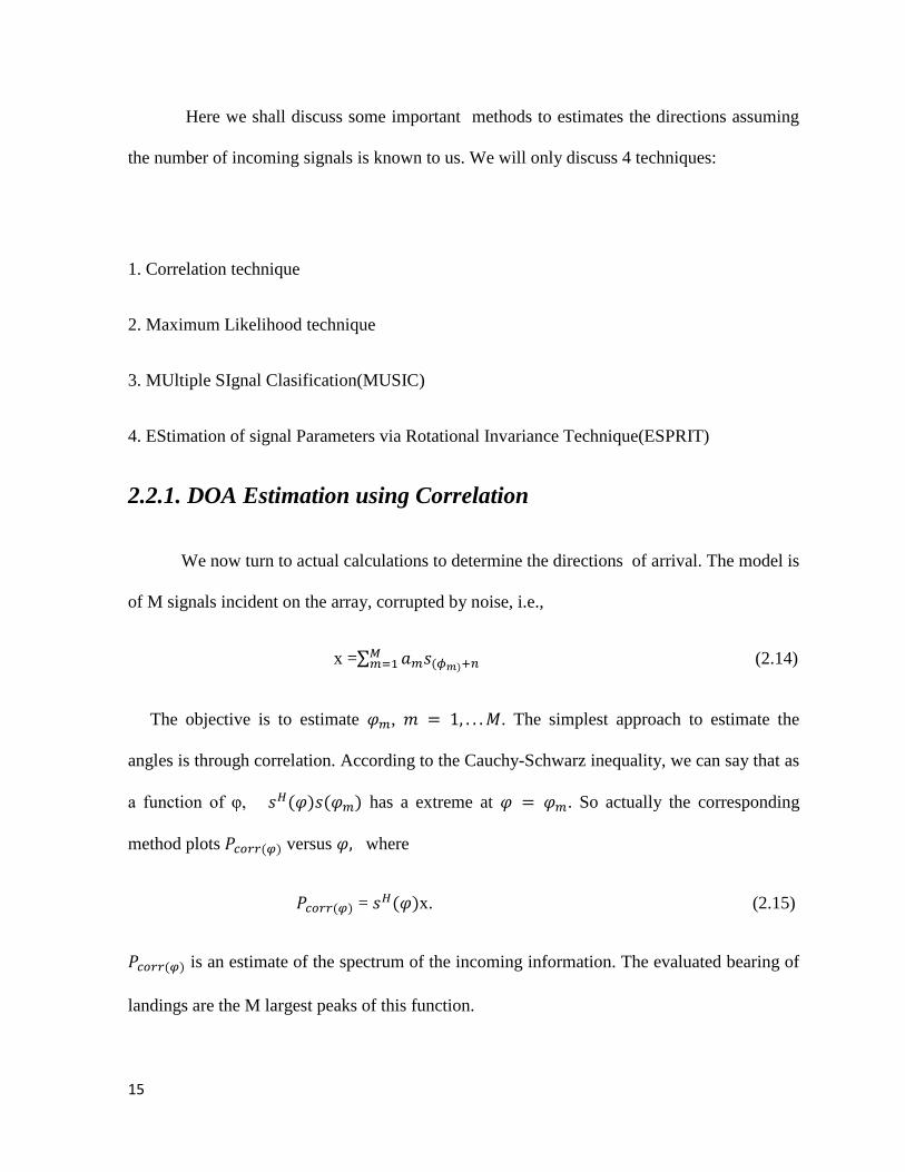
Here we shall discuss some important methods to estimates the directions assuming

the number of incoming signals is known to us. We will only discuss 4 techniques:

1. Correlation technique

2. Maximum Likelihood technique

3. MUltiple SIgnal Clasification(MUSIC)

4. EStimation of signal Parameters via Rotational Invariance Technique(ESPRIT)

2.2.1. DOA Estimation using Correlation

We now turn to actual calculations to determine the directions of arrival. The model is

of M signals incident on the array, corrupted by noise, i.e.,

x =∑ (2.14)

The objective is to estimate , . The simplest approach to estimate the

angles is through correlation. According to the Cauchy-Schwarz inequality, we can say that as

a function of φ, has a extreme at . So actually the corresponding

method plots versus where

= x. (2.15)

is an estimate of the spectrum of the incoming information. The evaluated bearing of

landings are the M largest peaks of this function.

16

2.2.2 DOA estimation using Maximum Likelihood Estimator

In this method DOA estimation is done of an incoming signal by maximizing the

probability of coming of a signal from a particular direction. The information model we utilise

is the same which is employed for correlation technique. The n vector is statistically colored

and, generally can be given as, [ ] .. The form of maximum likelihood estimator

(MLE) is

Ӫ, ᾶ= max[ ⁄ (x)], (2.16)

Where ⁄ (x) is the probability distribution function of the information matrix x when

parameters Ӫ,ᾶ are known. If the noise vector is Gaussian we can write

⁄ (x)=

, (2.17)

i.e, the maximization in eqn is analogous to

Ӫ,ᾶ=min[ ] ( 2.18)

=min[

]

We must get the minimum value of this function. For that first we are differentiating the

function w.r.t for finding the value of that will minimize the function.

=

=

(2.19)

17

Using this value of , we can calculate as

[ ] [|

|

] (2.20)

The function is the maximum probable estimate of the spectrum of the incoming

information. The extreme points of this function is the estimated DOAs.

An intriguing part of maximum probable estimator is that if there is single client and

= I, the only the diagonal elements of the correlation matrix is non-zero hence the MLE

is reduced to the corresponding strategy of Section 3. This is normal on the ground that the

correlation technique in that case is analogous to the matched filter, which is ideal in the

solitary user scenario .

2.2.3. MUSIC: MUltiple SIgnal Classification

MUSIC is most popular eigen decomposition based DOA estimation technique. The

received signal vector can be written as

. (2.21)

Where [ ] ,

And [ ] .

18

The matrix is a matrix of the steering or controlling vectors. For simplicity we

are accepting that the different signals are uncorrelated. The correlation matrix of the

received signal vector can be given as

[ ]

= [A ] [ ]

= +

= + (2.22)

Where

= and

a=[

[ ]

[ ]

[ ]

] (2.23)

The signal covariance matrix, , is obviously a matrix with rank M. So there are

eigenvectors that corresponds to the zero eigenvalue. Let qm be such an eigenvector in

relation to zero eigenvalue. Therefore it is feasible to write,

= Aa = 0,

⇒ Aa = 0,

⇒ = 0 (2.24)

This final equation is true as the matrix is obviously positive definite. Equation implies

that all eigenvectors ( ) of corresponding to the zero eigenvalues are orthogonal

19

to all M signal steering vectors. This is the underlying logic for MUSIC. (noise subspace)

is the matrix of these eigenvectors.

MUSIC actually plots the pseudo-spectrum

=

| |

(2.25)

As from the previous discussion it is conferred that the noise vector is orthogonal to signal

steering vector so for any signal direction becomes zero. Therefore, the estimated

signal directions are the M biggest crests in the pseudo-spectrum. One trick is that in reality

we will not be provided with the signal covariance matrix. We have to estimate that one. And

from that estimate of we have to calculate the noisy eigen vectors.

For any eigenvector ∈ ,

= λ

⇒ R = + I =( +

It is clear that. any eigenvector of is also an eigenvector of R with corresponding

eigenvalue . Letting = . We can write

R= [ ]

=Q

[

]

(2.26)

20

By this eigen splitting we will get two different matrix. One is called signal space containing

the eigen vectors of signal eigenvalues and the other is called noise space containing the

vector of noisy eigenvalues. is the signal subspace, and is the noise subspace.

There are few paramount perceptions to be made:

• The smallest eigenvalues of R are the noise eigenvalues and are all same to σ2,noise

covariance i.e., one way of recognizing the signal and noise eigenvalues (equivalently the

signal and noise subspaces) is to calculate the number of small eigenvalues that are equal.

• By orthogonality stated above it is logical to write for Q, ⊥

Considering the last two observations, we see that all noise eigenvectors are orthogonal

to the signal steering vectors. This is the logic behind MUSIC. Consider the following

function of φ:

= 1/ (

If is equal to DOA of any one of the signals, ⊥ and the denominator of the

function is zero. MUSIC, therefore, gives the peaks of the function ,as the directions

of arrival.

21

2.2.4 Estimation of Signal Parameters via Rotational Invariance

Technique(ESPRIT)

ESPRIT is another very popular high resolution DOA estimation technique .It uses

the fact that the signal at each member of the array is at constant phase shift from its earlier

element.

matrix of steering vectors given by

A=

[

]

Now we are incorporating two matrices, and A1, where

and A1 comprises the 1st rows of A and last rows of A.

[

]

[

]

Now we are defining another matrix ϕ with dimension

22

Φ =[

]

It can be verified that Φ by simple mathematics.

is a matrix of only diagonal elements, which correspond to the phase shift from

one element to the next. From the above equation it is clear that if we can estimate then we

will get desired incoming directions.

If and were known, we could get very easily. But we must resort an

indirect method to obtain the desired result as they are not known .

From the concept of linear algebra it can be said that the same subspace is covered by

the matrix (steering matrix) and the matrix (matrix of signal eigenvectors). So there is

existence of an unique invertible matrix T such that the following equation holds.

= (2.27)

Now partition of has been done in the similar way of partitioning of A. The first matrix

comprises the first rows of and the last (N − 1) rows of .

= , (2.28)

and

= = ΦT (2.29)

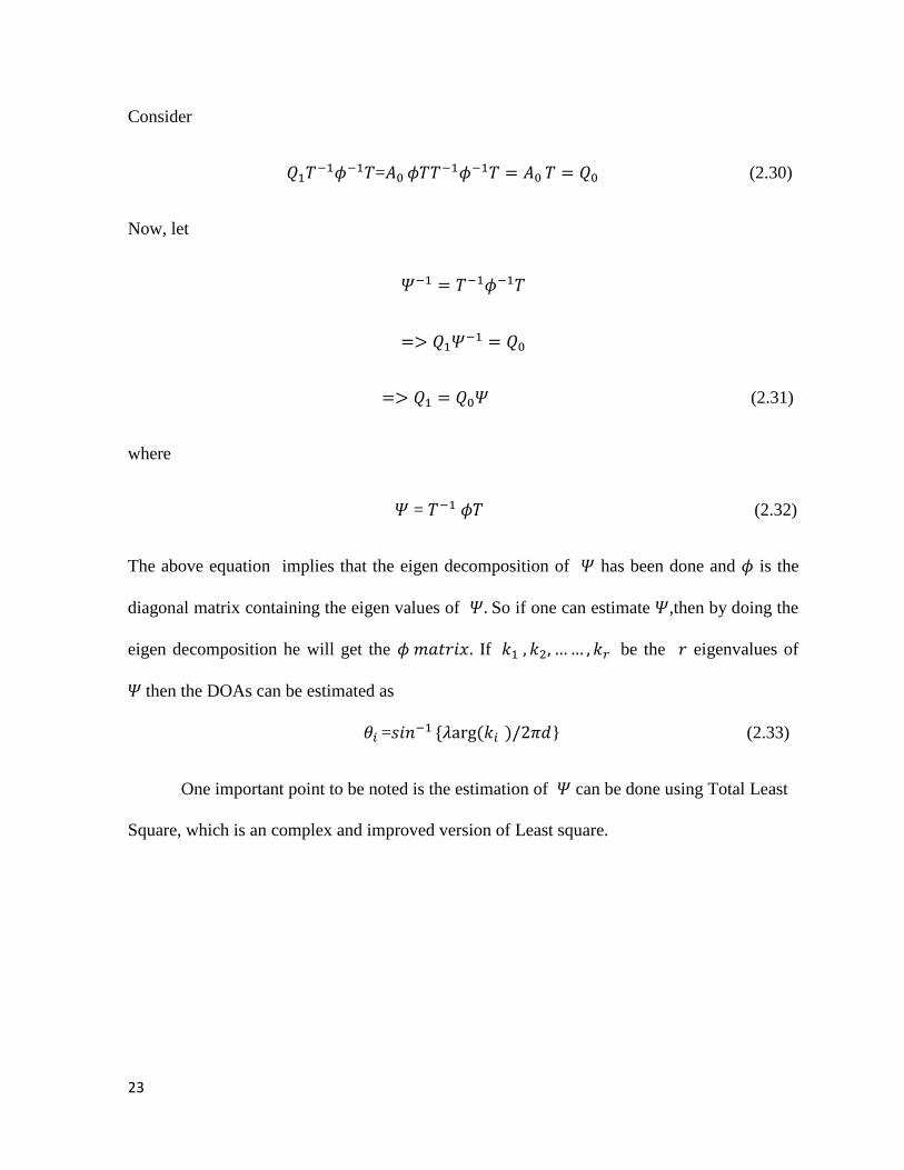
23

Consider

=

(2.30)

Now, let

(2.31)

where

= (2.32)

The above equation implies that the eigen decomposition of has been done and is the

diagonal matrix containing the eigen values of So if one can estimate ,then by doing the

eigen decomposition he will get the If be the eigenvalues of

then the DOAs can be estimated as

= } (2.33)

One important point to be noted is the estimation of can be done using Total Least

Square, which is an complex and improved version of Least square.

24

Chapter 3

Literature Review

Direction of Arrival (DOA) estimation finds its practical importance in sophisticated

video conferencing by audio visual means, locating underwater bodies, removing unwanted

interferences from desired signals etc. So considerable attention is there in recent research on

this area and various algorithms are getting developed for this purpose by various researchers.

It is found that the effective algorithms use sensor array processing in which a number of

sensors are used to receive the signals from various directions. Popularly used high resolution

methods for DOA estimation are MUltiple SIgnal Classification(MUSIC), root-MUSIC,

Estimation of Signal Parameters via Rotational Invariance Techniques (ESPRIT), and

Maximum Likelihood (ML) algorithm which use array signal processing[8]-[12]. In [13]

authors have estimated DOA of underwater target with acoustic array. For acoustic echo

detection generally time delay based algorithm is frequently used. But they have introduced

here adaptive phase difference estimator which works efficiently even with small array for

determining the angular location of closely spaced sources. The phase difference is obtained

by computing the adaptive weights of two parallel adaptive notch filters.

However, the above algorithms consider the ideal sensor array in which the

imperfections such as mutual coupling between sensors, gain and phase errors which are

obvious in practical scenario have not been taken into consideration . It has been found that

performance in DOA estimation degrade due to those imperfections as it alters the ideal

array manifold. Various techniques to combat those limitations for high frequency signals

25

are available in existing literature. An iterative eigen structure based method for direction

finding considering sensor mutual coupling , gain and phase uncertainties is given in[14].

Here along with DOAs mutual coupling coefficients, gain and phase errors have been

calculated. 1st the directions have been found by taking the assumption that the gain, phase

and mutual interaction parameters are in hand. After that using the results of DOAs they have

minimized a certain cost function with respect to gain and phase error parameters. In the 3rd

step they have again minimized that cost function to find the coupling coefficients, but this

time with respect to both DOAs and gain, phase coefficients. The minimization process is

repeated until they have got a sufficicent less value of the cost function. But they have not

formulated sufficient conditions for convergence of the cost function. DOA estimation of

multiple signals using uniform linear arrays with mutual coupling by setting the sensors at the

boundary as auxiliary sensors is found in existing literature [15]. It has been shown in that the

interaction between adjacent individuals with the same interspace is nearly equal, and the

magnitude of the mutual coupling coefficient between two far apart elements is so small that it

can be considered as null. Hence a banded symmetric Toeplitz matrix can be formed as model

for the mutual interaction of ULA. With that the authors have also considered the case of

coherent signal detection. They have compared two methods. 1st they have eliminated the

sensors at the boundary, spatial smoothing has been done on the middle subarray. 2nd

they

have applied the spatial smoothing in the whole subarray. And they have concluded that the

2nd

method gives better performance than the 1st one. Extension to uniform rectangular

array(URA) of the same problem statement as [15] has been done in [16] for estimating both

elevation and azimuthal angle of direction of arrival. They have proved that by setting the

outermost sensors as auxiliary sensors and taking the rest sensors into consideration will not

26

hamper the performance of 2-D MUSIC algorithm in a large way. Also they have used twice

search method to reduce the computational burden. Not only that, after getting the DOA

estimates they show how to get mutual coupling parameters utilizing those DOAs which is

not done in [15].They have even calculated CRLB(Cramer Rao Lower Bound).

Spatial smoothing has been introduced in [17 ] . This is a technique to alleviate

the problems faced when one trying to estimate the DOAs of fully correlated(coherent)

signals resulting from multipath propagation. A Relatively different problem of DOA

estimation for mixed signal (combination of correlated, uncorrelated and coherent signals)

has been addressed in [18].They have developed a two stage process.1st they have estimated

the DOAs of partially correlated and uncorrelated signals using any standard subspace

approach. Then by oblique projection method they have eliminated the effect of lowly

correlated and uncorrelated signals from the coherent signals. In the last step they DOAs of

the coherent sources have been found by spatial smoothing technique. If number of signals is

more than no of sensors then also their method works properly. But in this work they have

taken ideal sensor array in which there was no uncertainties. Estimation of DOAs for mixed

signls in the presence of mutual coupling has been studied in [19].Their procedure is partly

same as of [18].Here also they have estimated the direction of falling of the non-coherent

signls firstly. Using that information they have found the coupling coefficients by a lest

square solution. In the final step for getting the DOAs of coherent signals they have taken the

method of oblique projections to nullify the contribution of non coherent signals and also they

have reduced the effect of mutual interaction. Iterative search is not needed at all in their

method. With that they have shown the methodology to find the lost angles.

27

In [20] the authors have designed sensor imperfections as gain and phase errors.

DOA estimation in the presence of these unknown gain and phase error of the sensors

has been done using partly calibrated arrays. Partly calibrated array menas some of the array

elements are ideal means gain is unity and no phase shift is there between falling and reflected

signal. The conventional ESPRIT algorithm requires the fully calibrated array and the

subarrays be oriented in the same way. Unfortunately, the arrays we deal with in practice

may only be partly calibrated.As a result the ESPRIT algorithm cannot be directly applied . In

this estimation of DOAs are executed by a ESPRIT based method for partly calibrated array

along with the finding of unknown gain and phase coefficients by solving a optimization

problem without spectral search. In addition they have derived the CRLB of the RMSE. By

simulation results it is resoluted that the performance of this method is even better when the

no of uncalibrated sensors is large. Author in [21] presented a maximum-likelihood

calibration algorithm to compensate for the effect of mutual coupling, sensor gain and phase

errors. But it requires a set of calibration sources at known locations. Though this method

works efficiently with varying or changing uncertainties of array members but the

implementation of this method is costly . Authors in [22] –[25] discussed receiving mutual

impedance method for mutual coupling reduction.

Though in all these papers mutual coupling problem is addressed, that is done for

very high frequency signals. With few exceptions mutual coupling problem has not been

addressed in case of acoustic sensors due to their practical limitations and for less amount of

coupling for low frequency signals. Though J.W Pierre and M. Kaveh presented the

comparison between several DOA estimation algorithms using the University of Minnesota

Ultrasonic Sensor array testbed in[26] means The efficiency of various DOA estimation

28

procedure is investigated in hardware which was very rare in research paper. The array

comprises eight ultrasonic transducers operating at 40 kHz. So automatically they have faced

the nonideality of the practical arrays and as so they have also illustrated the calibration

procedure. They have compared Capons MLM, MUSIC, Root MUSIC, Min Norm, ESPRIT

and a weighted norm version of MUSIC .In simulation section they also provided the plot of

bias and variance of RMSE versus SNR. But effect of mutual coupling as the sources

becomes closer has not been addressed yet.

In this work our objective is to study the effect of coupling when spacing between the

acoustic sources varies. For simplicity we consider that the signals are uncorrelated. This

work has been motivated by the need to evaluate the performance of high resolution methods

in the presence of mutual coupling or to see upto which degree of resolution their working is

efficient. For that 1st we have estimated the DOAs using high resolution ESPRIT algorithm.

Then by least square solution we have estimated the coupling coefficients. With these known

coefficients we have got the more accurate DOA. Then we have compared the two results to

get an insight about the degradation of performance due to coupling.

We have taken four sets of acoustic signal sources of different resolutions and shown

the effect of coupling for different spacings.

29

Chapter 4

Effect of mutual coupling on DOA estimation

4.1 Formation of coupling matrix for DOA estimation

In this chapter the effect of mutual coupling on the DOA estimation performance has

been studied.

We are taking a ULA consists of alike acoustic sensors. The distance between

neighbouring elements of the array is . Suppose narrowband uncorrelated acoustic signals

fall on the array with angles at tth

time index.

Suppose C denotes the mutual interaction matrix for the ULA. Then the output

from the array sensors can be given as

(4.1)

where , A, and are the received signal vector, the ideal array manifold, the

signal 1-D matrix, and the noise 1-D matrix respectively.

=[ ] (4.2)

=[ ], (4.3)

[ ] , (4.4)

[ ] (4.5)

The ideal steering vector is expressed as

30

[

] (4.6)

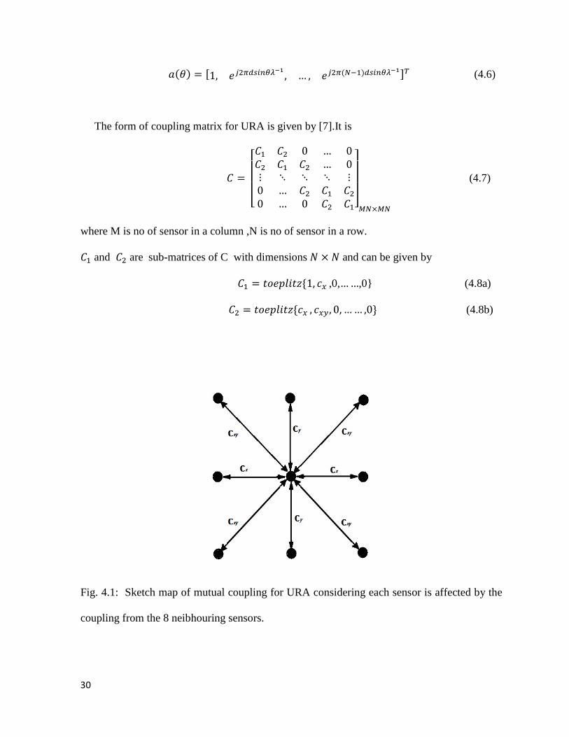
The form of coupling matrix for URA is given by [7].It is

[ ]

(4.7)

where M is no of sensor in a column ,N is no of sensor in a row.

and are sub-matrices of C with dimensions and can be given by

,0, ,0} (4.8a)

(4.8b)

Fig. 4.1: Sketch map of mutual coupling for URA considering each sensor is affected by the

coupling from the 8 neibhouring sensors.

31

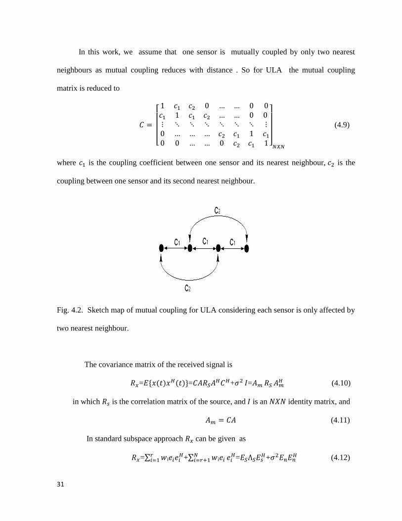
In this work, we assume that one sensor is mutually coupled by only two nearest

neighbours as mutual coupling reduces with distance . So for ULA the mutual coupling

matrix is reduced to

[ ]

(4.9)

where is the coupling coefficient between one sensor and its nearest neighbour, is the

coupling between one sensor and its second nearest neighbour.

Fig. 4.2. Sketch map of mutual coupling for ULA considering each sensor is only affected by

two nearest neighbour.

The covariance matrix of the received signal is

= = + =

(4.10)

in which is the correlation matrix of the source, and is an identity matrix, and

(4.11)

In standard subspace approach can be given as

=∑ i

+∑ i

= +

(4.12)

32

where ≥ ≥ ≥ > = = are the eigenvalues of received vector and the

respective eigenvectors are . and contains the eigenvectors associated

with the largest eigenvalues and smallest eigenvalues.

Now we are all prepared to estimate DOAs by ESPRIT using the mutually coupled

steering matrix. After that we shall estimate the coupling coefficients .Using those known

coefficients DOAs have been computed again. Then comparison of the results have been

done for different source spacing to observe the effect of mutual coupling as the source

spacing varies to see how much resolution can be achieved in practical application.

4.2 DOA estimation based on ESPRIT algorithm

We shall now estimate the DOAs using the mutually coupled steering vector. We

can divide the ULA into two overlapping subarrays where the first subarray comprises of

first (N-1) sensors and the second one consists of the last (N-1) sensors. Mutually coupled

steering matrices of these two subarrays are denoted as Am1 and Am2 .

It can be verified that the relation between and is

(4.13)

where are ideal steering vector and is an diagonal matrix , given by

= {

} (4.14)

As the span of signal subspace and the span of the steering matrix is same i.e,

span{ }=span{ },there exists an nonsingular matrix such that

(4.15)

33

Now we can partition the as and .So we have

(4.16a)

(4.16b)

After further manipulation

= (4.17)

where the matrix is given by

(4.18)

If be the eigenvalues of then the DOAs can be estimated as

= } (4.19)

After getting the DOAs ,suppose the new steering vector is which is a

matrix.So now we can find the mutual coupling coefficients by the method described in

[8]and can form the MCM matrix .

We can write (4.20)

Where is the sum of the following two matrices

[ ] ={[ ]

(4.21)

[ ] ={[ ]

(4.22)

Now

[

] [

] (4.23)

34

≜ ( ) (4.24)

Where is the noise subspace.

And we can get least square solution as

= [ ] (4.25)

Once we know C we are free to calculate nearly ideal steering matrix from the

equation

(4.26)

Using this (the recalculated steering vector after the calculation of MCM)we can again

compute the DOAs using ESPRIT algorithm which are nearer to the actual DOAs than the

DOAs found in the previous iteration.

4.3 Simulation Results

In order to observe the effect of mutual coupling on the algorithm simulation of a

ULA with N=15 sensors separated by d is done. We have taken four sets of three uncorrelated

narrowband acoustic signals (spacing of 20◦,10

◦,8◦ and 5

◦) with identical power.The

background noise is assumed to be Additive White Gaussian Noise(AWGN). The power of

the signal is ,noise power is and the input SNR of the signal is formulated as

10log10( ) in dB.

35

In this experiment , we take the mutual coupling parameters as = 0.107 - 0.1 ,

=-0.013+0.02 . No. of snapshots taken in each experiment is 300.For each SNR level the

same experiment is done 550 times. The RMSE of the estimated DOAs is calculated as

RMSE=√∑ ∑

where is the number of Monte-carlo experiments, is the signal source number and

is the nth

estimated DOA in the -th Monte-carlo experiment.

The RMSE versus SNR curve are illustrated in fig 4.3 for DOAs 10◦,30

◦,50

◦.It is

shown that there is a significant improvement in the DOA estimates for the 2nd

iteration in

which nearly ideal steering vector has been calculated after estimating the mutual coupling

coefficients.

Also RMSE versus SNR plots are illustrated in fig 4.4 for DOAs 10◦,20

◦,30

◦.The same

has been shown in fig 9 for DOAs 10◦,18

◦,20

◦.Further decrease of the spacing of sources the

system would not be able to compute DOAs of that sources due to large error. That case has

been shown in fig 10 for DOAs 10◦,15

◦,20

◦ .

In fig 6 the difference of RMSE in two iteration is about 0.04◦ (at 10 dB) whereas the

same is 0.1◦ and 0.15

◦ in fig 4.5 and fig 4.6 respectively. So it is evident that the degradation

in performance becomes more due to mutual coupling effect for more closely spaced sources.

36

Fig 4.3. RMSE of the estimated directions versus SNR of the signals coming from 10◦,30

◦,50

◦

Fig 4.4. RMSE of the estimated directions versus SNR of the signals coming from 10◦,20

◦,30

◦

-6 -4 -2 0 2 4 6 8 100.18

0.2

0.22

0.24

0.26

0.28

0.3

0.32RMSE vs SNR

SNR(in dB)

RM

SE

(in d

egre

e)

before mutual coupling reduction

after mutual coupling reduction

-6 -4 -2 0 2 4 6 8 100.08

0.1

0.12

0.14

0.16

0.18

0.2

0.22

0.24RMSE vs SNR

SNR(in dB)

RM

SE

(in d

egre

e)



37

Fig 4.5. RMSE of the estimated directions versus SNR of the signals coming from 10◦ 18

◦,26

◦

Fig 4.6. RMSE of the estimated directions versus SNR of the signals coming from 10

◦ 15

◦,20

◦

-6 -4 -2 0 2 4 6 8 100

0.05

0.1

0.15

0.2

0.25

0.3

0.35RMSE vs SNR

SNR(in dB)

RM

SE

(in

degree)



-6 -4 -2 0 2 4 6 8 100

0.5

1

1.5

2

2.5

3RMSE vs SNR

SNR(in dB)

RM

SE

(in d

egre

e)



38

Chapter 5

Effect of antenna gain and phase error on DOA estimation

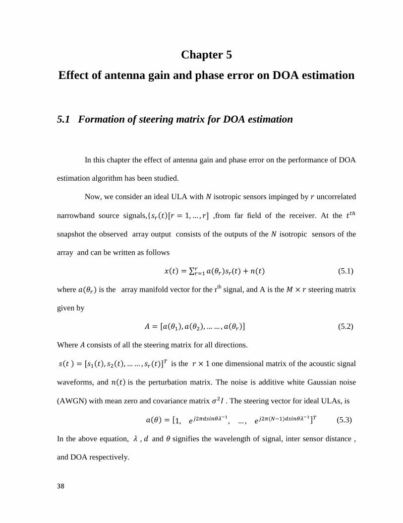
5.1 Formation of steering matrix for DOA estimation

In this chapter the effect of antenna gain and phase error on the performance of DOA

estimation algorithm has been studied.

Now, we consider an ideal ULA with isotropic sensors impinged by uncorrelated

narrowband source signals,{ [ ] ,from far field of the receiver. At the

snapshot the observed array output consists of the outputs of the isotropic sensors of the

array and can be written as follows

∑ ( (5.1)

where is the array manifold vector for the rth

signal, and A is the steering matrix

given by

[ ] (5.2)

Where consists of all the steering matrix for all directions.

[ ] is the one dimensional matrix of the acoustic signal

waveforms, and is the perturbation matrix. The noise is additive white Gaussian noise

(AWGN) with mean zero and covariance matrix . The steering vector for ideal ULAs, is

[

] (5.3)

In the above equation, , and signifies the wavelength of signal, inter sensor distance ,

and DOA respectively.

39

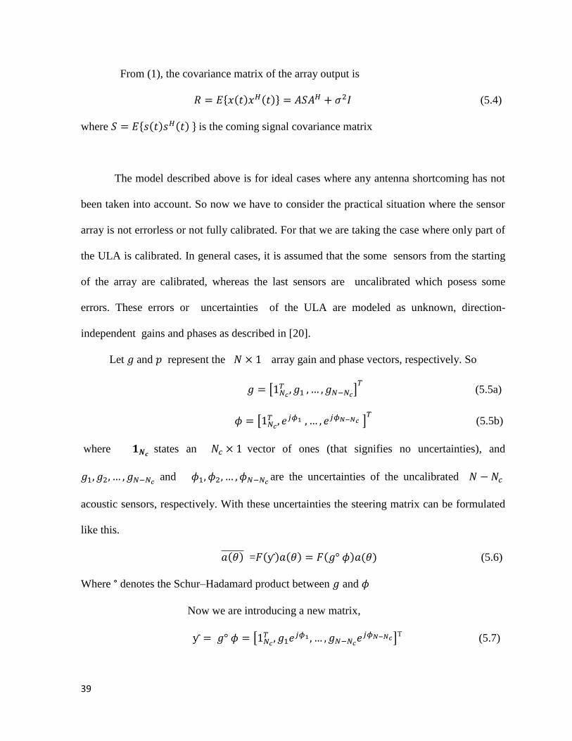
From (1), the covariance matrix of the array output is

(5.4)

where is the coming signal covariance matrix

The model described above is for ideal cases where any antenna shortcoming has not

been taken into account. So now we have to consider the practical situation where the sensor

array is not errorless or not fully calibrated. For that we are taking the case where only part of

the ULA is calibrated. In general cases, it is assumed that the some sensors from the starting

of the array are calibrated, whereas the last sensors are uncalibrated which posess some

errors. These errors or uncertainties of the ULA are modeled as unknown, direction-

independent gains and phases as described in [20].

Let and represent the array gain and phase vectors, respectively. So

[ ]

(5.5a)

[ ]

(5.5b)

where states an vector of ones (that signifies no uncertainties), and

and are the uncertainties of the uncalibrated

acoustic sensors, respectively. With these uncertainties the steering matrix can be formulated

like this.

= (5.6)

Where ° denotes the Schur–Hadamard product between and

Now we are introducing a new matrix,

[

]T

(5.7)

40

and is an diagonal matrix. Hence, the array covariance

matrix becomes

(5.8)

where is the array manifold of the partly calibrated or non ideal ULA. The

subspace decomposition (EVD) of R is

(5.9)

where is an diagonal matrix. Its elements are largest eigenvalues . is an

diagonal matrix. And its elements are smallest eigenvalues. is

the signal subspace matrix which carries the eigenvectors associated with the

largest signal eigenvalues, while is the noise subspace matrix containing the

eigenvectors related to the smallest noisy eigenvalues. For finite snapshots, the array

covariance matrix is

∑

Which can be decomposed further as

+ (5.10)

N is the number of time instant when the signal is sampled.

5.2 DOA estimation using non-ideal steering matrix

We are now prepared to estimate the DOAs using the partly calibrated ULA. As of

conventional ESPRIT (with full calibrated array), we divide the nonideal ULA into two

41

subarrays. The first subarray comprises of the first sensors, and the second comprises

of the last sensors. Also the steering matrix can be subdivided and the same for these

subarrays is given as following

(5.11a)

(5.11b)

and are the ideal steering matrices of the 1st and 2

nd subarrays respectively. and

are the ( error coefficient vectors of these two subarrays, and can be written in

the following manner.

[

]T

(5.12a)

[

]T

(5.12b)

By simple mathematic it can be shown that and satisfy

(5.13)

= {

} and it is a matrix.

Since spans the same subspace as the modified steering matrix

,i.e.,span{ span{ ,there exists an unique nonsingular matrix such that

(5.14)

Now we are dividing the signal suspace into 2 parts. Let first rows of forms ,

and the last rows of forms .

So we have

(5.15a)

(5.15b)

42

Since the matrices , ,and are nonsingular, by substituting (12) into (15) we get

(5.16)

where the matrix is given by

(5.17)

and with is an vector as following

[

( )] (5.18)

Here,we note that the as the first few elements are calibrated ,first elements

of are equal to one,

i.e., =1,

By the concepts of linear algebra we can say that and are similar matrices.

Therefore, the eigenvalues of must be equal to the diagonal elements of . If We denote

be the eigenvalues of , then the DOAs can be estimated by the following

equation,

(5.19)

These are the DOAs we have got by partly calibrated arrays. Also we have estimated

the DOAs using conventional ESPRIT algorithm taking ideal steering matrix means

considering the full calibrated array. We have compared the two results for partly calibrated

array and full calibrated array to show the degradation in performance in presence of antenna

error.

43

5.3 Simulation Results

For observing the effect of antenna gain and phase error on the algorithm, simulation

of a ULA consists N=10 elements separated by half a wavelength is run. We have taken four

sets of three uncorrelated narrowband acoustic signals(spacing of 12◦,10

◦,8◦ and 5

◦) with

identical power. If the power of the signal is and noise power is then the SNR is

10log10( ) in dB.

In the following simulation ,we have considered that the first three sensors are

calibrated and the rests are uncalibrated with unknown gain and phase errors given by

1.8 ,0.4 0.8 ,1.36 . No. of snapshots

taken in each experiment is 300.For each SNR level the same experiment is done 550 times.

The RMSE of the DOAs is calculated as

RMSE=√∑ ∑

where is the number of experiments, signal number is r and denotes the nth

estimated

DOA in the -th experiment.

The RMSE versus SNR curve are illustrated in fig 5.1 for DOAs 20◦,32

◦,44

◦.It is

shown that there is a significant improvement in the DOA estimates for the 2nd

iteration in

which ideal steering vector has been taken aS in the case of full calibrated array.

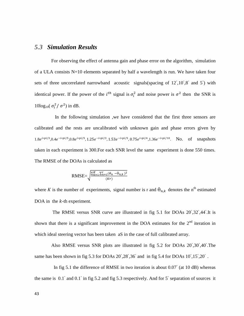
Also RMSE versus SNR plots are illustrated in fig 5.2 for DOAs 20◦,30

◦,40

◦.The

same has been shown in fig 5.3 for DOAs 20◦,28

◦,36

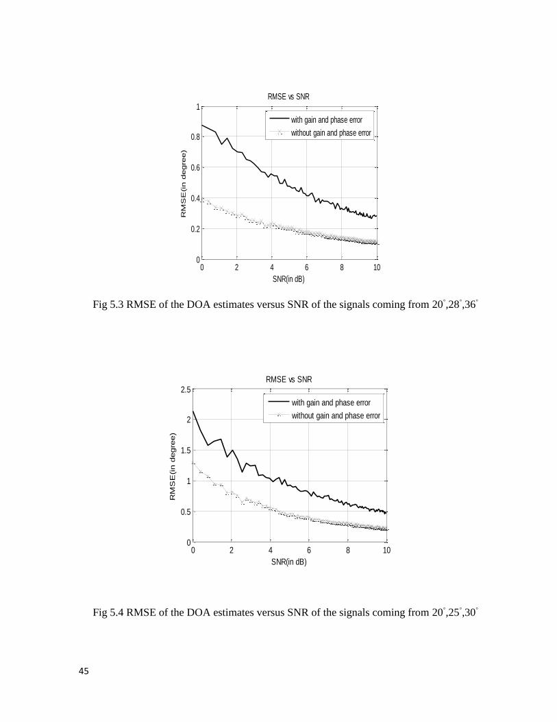
◦ and in fig 5.4 for DOAs 10

◦,15

◦,20

◦ .

In fig 5.1 the difference of RMSE in two iteration is about 0.07◦ (at 10 dB) whereas

the same is 0.1◦ and 0.1

◦ in fig 5.2 and fig 5.3 respectively. And for 5

◦ separation of sources it

44

is 0.2◦ .So it is evident that the degradation in performance becomes more due to antenna gain

and phase errors for more closely spaced sources.

Fig 5.1 RMSE of the estimated directions versus SNR of the signals coming from 20◦,32

◦,44

◦

Fig 5.2 RMSE of the estimated directions versus SNR of the signals coming from 20◦,30

◦,40

◦

0 2 4 6 8 100

0.1

0.2

0.3

0.4

0.5RMSE vs SNR

SNR(in dB)

RM

SE

(in d

egre

e)

with gain and phase error

without gain and phase error

0 2 4 6 8 100

0.1

0.2

0.3

0.4

0.5

0.6

0.7RMSE vs SNR

SNR(in dB)

RM

SE

(in d

egre

e)



45

Fig 5.3 RMSE of the DOA estimates versus SNR of the signals coming from 20◦,28

◦,36

◦

Fig 5.4 RMSE of the DOA estimates versus SNR of the signals coming from 20◦,25

◦,30

◦

0 2 4 6 8 100

0.2

0.4

0.6

0.8

1RMSE vs SNR

SNR(in dB)

RM

SE

(in d

egre

e)



0 2 4 6 8 100

0.5

1

1.5

2

2.5RMSE vs SNR

SNR(in dB)

RM

SE

(in d

egre

e)



46

Chapter 6

Conclusion

6.1 Conclusion

By a very simple iterative algorithm based on ESPRIT, it is shown that unknown

mutual coupling degrades the performance of DOA estimation algorithm. Moreover using the

four simulation results it is shown that the error due to coupling effect increases as the source

becomes closer and beyond a certain resolution the system fails to estimate the DOAs correctly.

Also for antenna gain and phase error it is evident from the simulation results that the

degradation in performance is more if the sources become closer. In this case also beyond a

certain limit system fails to give correct DOAs.

6.2 Future work

1) The effect of changing the no of calibrated sensors, increasing the no of snapshots

etc in the performance of the algorithms, can be studied.

2) Same work can be extended for URA and UCA also which are another two sensor

array structure mostly used for DOA estimation.

3) Mathematical model can be given to estimate properly the amount of degradation as

the sources becomes closer.

47

REFERENCES

[1]. Y. Huang, J. Benesty, and G. W. Elko, “Microphone Arrays for Video Camera Steering,”

Acoustic Signal Processing for Telecommunications , ed. S. L. Gay and J. Benesty,

Kluwer Academic Publishers, 2000.

[2]. C. Wren, A. Azarbayejani, T. Darrell, and A. Pentland, “Pfinder: Real-time tracking of

the human body,” Proc. on Automatic Face and Gesture Recognition, 1996, pp. 51-56.

[3]. M. S. Brandstein and S. M. Griebel, “Nonlinear, model-based microphone array speech

enhancement,” Acoustic Signal Processing for Telecommunications, ed S. L. Gay and J

Benesty, Kluwer Academic Publishers , 2000.

[4]. J. H. DiBiase, H. F.Silverman, and M. Brandstein, “ Robust Localization in Reverberant

Rooms,” Microphone Arrays, Springer- Verlag, 2001.

[5]. B. V. Veen and K. M. Buckley, “Beamforming Techniques for Spatial Filtering ,” CRC

Digital Signal Processing Handbook, 1999.

[6]. H. Kamiyanagida, H. Saruwatari, K. Takeda, and F. Itakura, “ Direction of arrival

estimation based on non-linear microphone array,” IEEE Conf. On Acoustics, Speech

and Signal Processing, Vol. 5, pp. 3033-3036, 2001.

[7]. C. H. Knapp and G. C. Carter, “ The Generalized Correlation Method for Estimation of

Time Delay,” IEEE Trans. Acoustics, Speech and Signal Proc., vol. ASSP - 24, No. 4,

August 1976.

[8]. R. O. Schmidt , “ Multiple emitter location and signal parameter estimations,”

IEEE Trans. Antenna Propag ., vol. AP- 34, no. 3, pp. 276- 280, Mar. 1986 .

[9]. A. J. Barabell , “ Improving the resolution performance of Eigen structure based

direction finding algorithms,” in Proc ICASSP, Boston, MA, May 1983, pp. 336-339.

[10]. R . Roy and T. Kailath, “ESPRIT-Estimation Of signal parameters via Rotational

invariance technique ,” IEEE Trans Acoustic Speech Signal Process., vol.37, no.7,

pp.984-995,Jul. 1989.

48

[11] Benjamin Friedlander , “ A sensitivity analysis of MUSIC algorithm, ” IEEE

Transaction on Acoustics,Speech and Signal Processing, vol 38, no 10.pp 1740-1751

[12]. P. Stoica , A. Nehorai, “ MUSIC , maximum likelihood, and Cramer Rao Bound,”

IEEE Trans Acoust., Speech, signal Process., vol. 37, no-5, pp.-720-741, May. 1989

[13]. CHEN Shao - hua , ZHENG Wei, LUO Hui-bin, ” Improved DOA estimation of

Underwater Target with Acoustic Cross Array,”ICSP-2012 Proceedings, pp. 2071-

2074,Mar 2012

[14]. Benjamin Friedlander and Anthony J. Weiss, “ Direction Finding in the Presence

of Mutual Coupling , ” IEEE Trans Antennas Propagation” ,vol. 39, no. 3, pp 273–

284, Mar.1991.

[15] . B. Liao and S. C. Chan,“ DOA estimation of Coherent Signals for Uniform Linear

Arrays With Mutual coupling ,” IEEE International Symposium on circuits and

systems, Reo de Janeiro,15-19 May 2011, pp. 377-380.

[16] Zhongfu Ye and Chao Liu, “ 2-D DOA Estimation in the presence of Mutual

Coupling,” IEEE Trans. Antennas Propagation. vol 56,no. 10, pp. 3150-3158, Oct.

2008.

[17] T. J.Shan , M.Wax , and T.Kailath, “On spatial smoothing for directional of arrival

estimation of coherent signals,” IEEE Trans.Acoust., Speech, Signal Processing, vol.

ASSP-33, pp-806–811, 1985.

[18] Xu X, Ye Z, Peng J. Method of direction of arrival estimation for uncorrelated,

Partially correlated and coherent sources.IET Microw.Antennas Propag. 2007, 1(4):

949-954.

[19] Xu Xu, Zhongfu Ye, and Yufeng Zhang , “ DOA estimation for Mixed signals in

the Presence of mutual coupling,” IEEE Trans Signal Processing, vol.57, no. 9, pp.

3523-3532,Sep. 2009.

[20] Bin Liao and Shing Chow Chan, “Direction finding with Partly Calibrated

Uniform Linear Arrays,” IEEE Trans Antennas Propagation .,vol.60, no.2, pp.922-

929 ,Feb 2012.

[21] B. C. Ng and C. M. S. See, “ Sensor Array Calibration Using a maximum

likelihood Approach,” IEEE Trans.Antenna Propag,Vol.44, pp .827-835, Jun. 1996.

49

[22] Y.Yu, H.S.Lui and H.T.Hui, “ Improved DOA estimation using the receiving mutual

Impedance for mutual coupling compensation : An experimental study” , IEEE

Transaction on Wireless Communication, vol 10,no 7, pp 2228-2233,2011

[23] Hon Tat Hui, “ A practical approach to compensate for the mutual coupling effect

in an Adaptive Dipole Array,” IEEE Transaction on Antennas and Propagation ,

vol 52, no 5 , pp. 1262-1269, May 2004

[24] Tong Tong Jhang ,Hon Tat Hui,Y.L.Lu,“Compensation for the mutual coupling effect

In the ESPRIT direction finding algorithm by using a more effective method ,” IEEE

Transaction on Antenna and Propagation, vol. 53, no 4,pp 1552-1555,Apr 2005

[25] Zhongfu Ye, Chao Liu, “ On the Resiliency of MUSIC direction finding against

antenna sensor coupling “IEEE Transaction on Antenna and Propagation , vol 56,

no 2, pp 371-380, Feb 2008

[26] J. W. Pierre and M. Kaveh, 1995. “Experimental Evaluation of high - Resolution

Direction Finding algorithms Using a Calibrated Sensor array testbed,”.Digital

Signal Processing, 5(4), pp. 243-254.

50

Publication

1) Anurag Patra, L.P.Roy, “Estimation of DOAs of Acoustic Sources with Different

Spacing in the Presence of Mutual Coupling,” IEEE International Conference on

Advanced Communication Control and Computing Technologies (ICACCCT), pp. 1021-

1024, May 2014

Estimation of DOAs of Acoustic Sources in the Presence of...

Documents

Transcript of Estimation of DOAs of Acoustic Sources in the Presence of...