1

ESTIMATION OF DELAY PROPAGATION IN THE NATIONAL AVIATION SYSTEM USING BAYESIAN NETWORKS

Ning Xu, George Donohue, Kathryn Blackmond Laskey, Chun-Hung Chen Department of Systems Engineering and Operations Research, George Mason University,

4400 University Drive, Fairfax, VA 22030-4444

Abstract Flight delay creates major problems in the

current aviation system. Methods are needed to analyze the manner in which micro-level causes propagate to create system-level patterns of delay. Traditional statistical methods are inadequate to the task. This paper proposes the use of Bayesian networks (BNs) to investigate and visualize propagation of delays among airports. The BN structure was developed from expert judgment and validated against empirical data. Parameters were estimated using a novel empirical Bayes approach in which regression estimates were used to construct a Dirichlet prior distribution, which was then updated from multinomial samples. Empirical results demonstrate greater predictive accuracy using our empirical Bayes approach than linear regression or Bayesian analysis with non-informative prior distributions. Our results clearly demonstrate the value of Bayesian networks for analyzing and visualizing how system-level effects arise from subsystem-level causes.

Introduction The National Aviation System (NAS) is a large

and complex stochastic system with thousands of interrelated components: administration, control centers, airports, airlines, aircraft, passengers, etc. The complexity of the NAS creates numerous difficulties in management and control. Among the most intractable of these problems is flight delay, with its attendant high cost to airlines, complaints from passengers, and difficulties for airport operations. Understanding and mitigating delays is a major long-term objective of the Federal Aviation Administration (FAA). As demand on the system increases, the delay problem becomes more and more prominent.

A great deal of research attention has been devoted to identifying the causes of delay. Major contributing factors to delay are congestion at the

origin airport, convective weather, reduced ceiling and visibility, continuously increasing demand and even changes in air traffic management (ATM) initiatives such as Ground Delay Programs (GDP). [7][8][9] Because the NAS is a stochastic control system, it must be characterized by probability density functions, and statistical analysis methods are necessary. Traditional linear and nonlinear regression methods have been applied to understand and explain the influences of weather, demand and other factors in the NAS system. [1][2] However, application of these methods has generally been limited to either single-airport analyses or aggregate analysis of the whole system. There is a need for a methodology powerful enough to represent and analyze the impact of micro airport-level causes on macro system-level performance.

Our new methodology combines multiple individual-airport Bayesian network models into a system-level model capable of representing interactions between airports. The system-level model provides a means of estimating interactions among delays at different airports. Three busy airports were selected for this study: Chicago O'Hare International Airport (ORD), LA Guardia Airport (LGA), and Hartsfield Atlanta International Airport (ATL). ORD and LGA are treated as originating airports and ATL is treated as the destination airport. We focus on investigating and quantifying how flight delays from a single airport propagate to impact other airports. Our methodology was applied to the analysis of historical data from November 2003 to January 2004.

Bayesian networks have become an increasingly important tool for investigating interdependence among multiple factors in complex systems. Bayesian networks have unique strengths both for inference and for visualization. When Bayesian networks are combined with traditional statistical methods, conditional independence can be exploited to provide more accurate estimation and therefore more precise prediction.

2

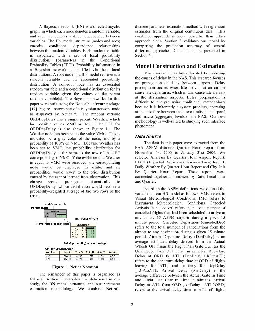
A Bayesian network (BN) is a directed acyclic graph, in which each node denotes a random variable, and each arc denotes a direct dependence between variables. The BN model structure (nodes and arcs) encodes conditional dependence relationships between the random variables. Each random variable is associated with a set of local probability distributions (parameters in the Conditional Probability Tables (CPT)). Probability information in a Bayesian network is specified via these local distributions. A root node in a BN model represents a random variable and its associated probability distribution. A non-root node has an associated random variable and a conditional distribution for its random variable given the values of the parent random variable(s). The Bayesian networks for this paper were built using the Netica™ software package [12]. Figure 1 shows part of a Bayesian network node as displayed by Netica™. The random variable ORDDepDelay has a single parent, Weather, which has possible values VMC or IMC. The CPT for ORDDepDelay is also shown in Figure 1. The Weather node has been set to the value VMC. This is indicated by a gray color of the node, and by a probability of 100% on VMC. Because Weather has been set to VMC, the probability distribution for ORDDepDelay is the same as the row of the CPT corresponding to VMC. If the evidence that Weather is equal to VMC were removed, the corresponding node would be displayed in white, and its probabilities would revert to the prior distribution entered by the user or learned from observation. This change would propagate automatically to ORDDepDelay, whose distribution would become a probability-weighted average of the two rows of the CPT.

Figure 1. Netica Notation

The remainder of this paper is organized as follows. Section 2 describes the data used in our study, the BN model structure, and our parameter estimation methodology. We combine Netica’s

discrete parameter estimation method with regression estimates from the original continuous data. This combined approach is more powerful than either approach alone. Section 3 validates our model by comparing the prediction accuracy of several different approaches. Conclusions are presented in Section 4.

Model Construction and Estimation Much research has been devoted to analyzing

the causes of delay in the NAS. This research focuses on propagation of delay between airports. Delay propagation occurs when late arrivals at an airport cause late departures, which in turn cause late arrivals at the destination airports. Delay propagation is difficult to analyze using traditional methodology because it is inherently a system problem, operating at the interface between the micro (individual airport) and macro (aggregate) levels of the NAS. Our new methodology is well-suited to studying such interface phenomena.

Data Source The data in this paper were extracted from the

FAA ASPM database Quarter Hour Report from November 1st 2003 to January 31st 2004. We selected Analysis By Quarter Hour Airport Report, EDCT (Expected Departure Clearance Time) Report, Daily Weather By Quarter Hour Report and City Pair By Quarter Hour Report. These reports were connected together and indexed by Date, Local hour and Quarter.

Based on the ASPM definitions, we defined the variables in our BN model as follows. VMC refers to Visual Meteorological Conditions. IMC refers to Instrument Meteorological Conditions. Canceled Arrivals (canceledArr) refers to the total number of cancelled flights that had been scheduled to arrive at one of the 55 ASPM airports during a given 15 minute period. Canceled Departures (canceledDep) refers to the total number of cancellations from the airport to any destination during a given 15 minute period. Airport Departure Delay (DepDelay) is an average estimated delay derived from the Actual Wheels Off minus the Flight Plan Gate Out less the Unimpeded Taxi Out Time, in minutes. Departure Delay at ORD to ATL (DepDelay_ORDtoATL) refers to the departure delay time at ORD of flights leaving for ATL, and similarly for DepDelay _LGAtoATL. Arrival Delay (ArrDelay) is the average difference between the Actual Gate In Time and Flight Plan Gate In Time in minutes. Arrival Delay at ATL from ORD (ArrDelay _ATLfrORD) refers to the arrival delay time at ATL of flights

3

coming from ORD, and similarly for ArrDelay _ATLfrLGA. Delay values may be negative, due to the fact that flights may arrive or depart early.

To introduce different time phases into our model, we create “advance” data by connecting the departure data at ORD and LGA with arrival data at ATL after a given period of time. For example, to study the impact of departure delays at ORD between 6:00am and 6:15am on the arrival delay at ATL 2 hours later, we connect the 6:15am ORD data with 9:15am ATL data. (The 3-hour difference is due to a 1-hour time zone difference and a 2-hour flight time.) Through this process, we created advance variables ArrDelay_ATLfrORD+2:00, ATLArrDelay+2:00, and so forth.

We selected a sub-sample of 90% of the observations to build our model structure and to estimate parameters. The remaining 10% of the data points were set aside to test the accuracy of model predictions.

Model Structure Our initial BN model structure was developed

using expert judgment. A statistical significance test was then conducted on pairs of nodes connected by an arc in the expert-elicited BN. Associations between the nodes in the structure listed below were statistically significant at level 0.05.

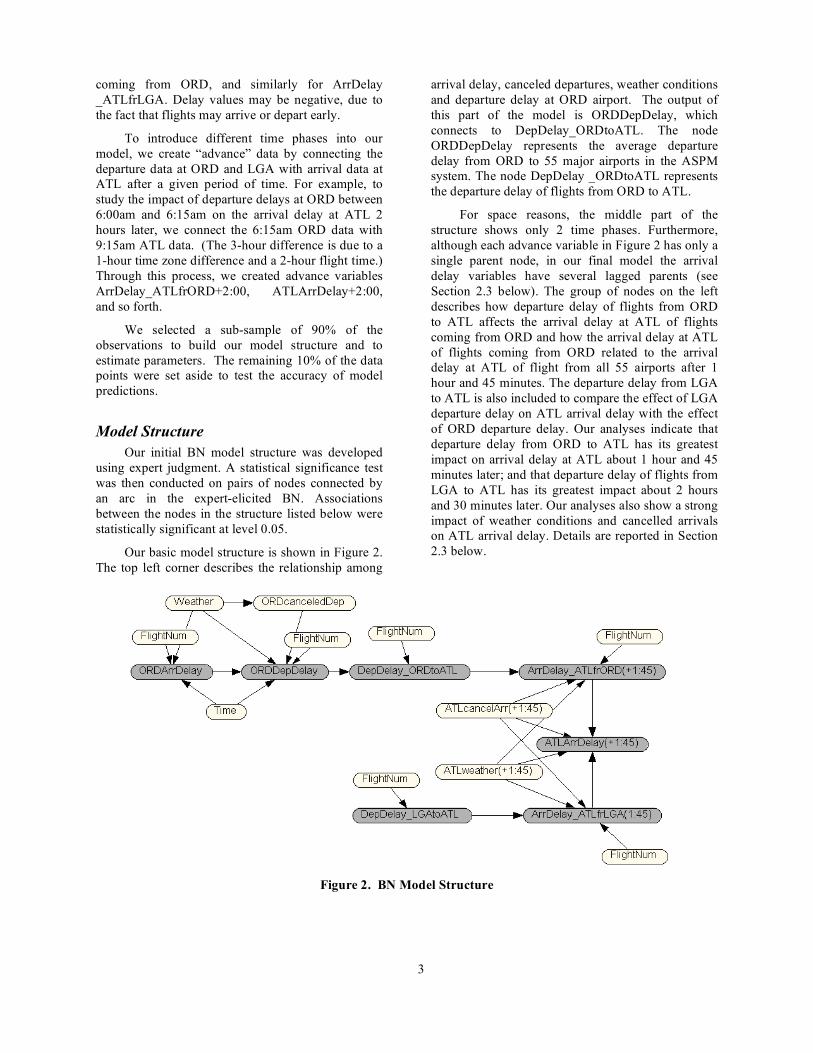
Our basic model structure is shown in Figure 2. The top left corner describes the relationship among

arrival delay, canceled departures, weather conditions and departure delay at ORD airport. The output of this part of the model is ORDDepDelay, which connects to DepDelay_ORDtoATL. The node ORDDepDelay represents the average departure delay from ORD to 55 major airports in the ASPM system. The node DepDelay _ORDtoATL represents the departure delay of flights from ORD to ATL.

For space reasons, the middle part of the structure shows only 2 time phases. Furthermore, although each advance variable in Figure 2 has only a single parent node, in our final model the arrival delay variables have several lagged parents (see Section 2.3 below). The group of nodes on the left describes how departure delay of flights from ORD to ATL affects the arrival delay at ATL of flights coming from ORD and how the arrival delay at ATL of flights coming from ORD related to the arrival delay at ATL of flight from all 55 airports after 1 hour and 45 minutes. The departure delay from LGA to ATL is also included to compare the effect of LGA departure delay on ATL arrival delay with the effect of ORD departure delay. Our analyses indicate that departure delay from ORD to ATL has its greatest impact on arrival delay at ATL about 1 hour and 45 minutes later; and that departure delay of flights from LGA to ATL has its greatest impact about 2 hours and 30 minutes later. Our analyses also show a strong impact of weather conditions and cancelled arrivals on ATL arrival delay. Details are reported in Section 2.3 below.

Figure 2. BN Model Structure

4

Parameter Estimation Initial exploratory parameter estimation was

performed using Netica’s parameter learning capability. Netica’s parameter learning assumes multinomial random variables with Dirichlet conjugate prior distributions. This method is appropriate for categorical random variables, when parameters for different categories are unrelated. Many of our random variables are continuous, and were discretized for representation in Netica. Parameters associated with neighboring discretized categories are expected to be similar. For this reason, multinomial / Dirichlet estimation has less statistical power than could be achieved with a more sophisticated approach. Nevertheless, the estimates were useful for exploratory purposes – to compute initial parameter estimates and to visualize delay propagation among airports.

Our exploratory analyses used a uniform prior distribution, that is: ),( ,1 pDirichlet !! ! where

1,1 === p!! ! , and =p number of states. This prior distribution places equal density on all possible states for each node in the model. Because the Dirichlet prior is conjugate to the multinomial distribution, the posterior distribution can be obtained in closed form. After

in cases have been observed

for a random variable given particular values for its parents, the posterior distribution is ),,( 11 pp nnDirichlet ++ !! ! . The posterior expected value of the ith state for the given configuration of parents is ! ++ )(/)(

iiiinn "" .

While this analysis was useful for exploratory purposes, there are several reasons why a more sophisticated model is necessary. As noted above, the multinomial / Dirichlet analysis requires the data to be discretized. While sophisticated discretization methods exist [12], we used human judgment to discretize our data.

More significantly, in the multinomial / Dirichlet model, each probability in a belief table is estimated independently of all the other probabilities. For continuous random variables, probabilities of nearby states are expected to be near each other. Ignoring these relationships wastes statistical power. Even with a relatively coarse discretization, there may be very few observations for some configurations of a random variable’s parents. For such configurations, parameter estimates are highly imprecise. Methods that incorporate information

about nearby parent configurations provide much greater statistical power.

Our second step estimates the parameters using regression analysis. We plotted pairs of delays to ascertain whether the relationship was linear. If so, linear regression was applied to estimate the relationship between parent and child random variables. For example, if node D has parent nodes A and B, and the states of D are linearly related to the states of A and B, then the probability of states of node D given A and B was specified using Netica’s NormalDist function:

),,(),|( 21 !""# BADNormalDistBADP ++= , where BA

21!!" ++ is the mean of the normal

distribution ),|( BADP , and σ is the standard deviation.

We used the statistical package SAS to estimate the parameters !""# ,,, 21 , and entered the parameter estimates into a Netica equation. Netica converted the equation into a conditional probability table for the discretized random variable. We then used this generated CPT (with a virtual count of 1) as the Dirichlet prior distribution. That is, the prior distribution was ),( ,1 pDirichlet !! ! , where αi is

the probability given by the above regression equation that an observation falls into the ith bin. The posterior distribution is, as before,

),,( 11 pp nnDirichlet ++ !! ! .

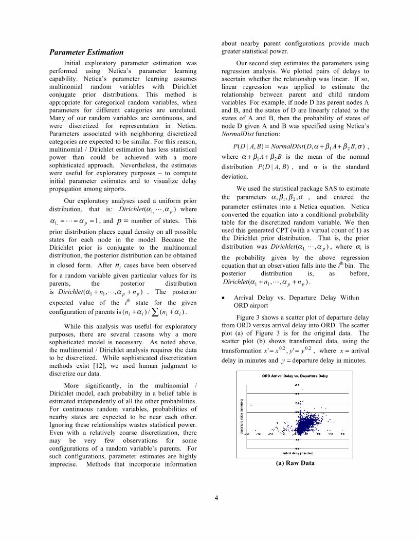
• Arrival Delay vs. Departure Delay Within ORD airport

Figure 3 shows a scatter plot of departure delay from ORD versus arrival delay into ORD. The scatter plot (a) of Figure 3 is for the original data. The scatter plot (b) shows transformed data, using the transformation 2.02.0

',' yyxx == , where =x arrival delay in minutes and =y departure delay in minutes.

(a) Raw Data

5

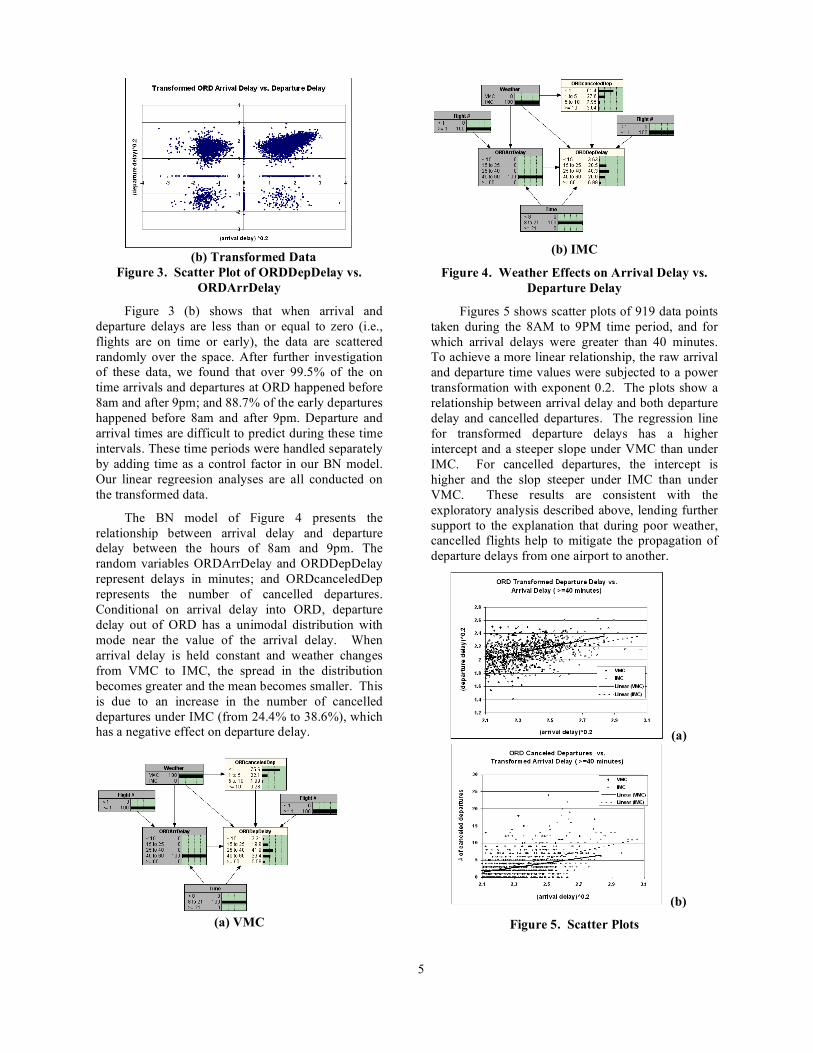
(b) Transformed Data

Figure 3. Scatter Plot of ORDDepDelay vs. ORDArrDelay

Figure 3 (b) shows that when arrival and departure delays are less than or equal to zero (i.e., flights are on time or early), the data are scattered randomly over the space. After further investigation of these data, we found that over 99.5% of the on time arrivals and departures at ORD happened before 8am and after 9pm; and 88.7% of the early departures happened before 8am and after 9pm. Departure and arrival times are difficult to predict during these time intervals. These time periods were handled separately by adding time as a control factor in our BN model. Our linear regreesion analyses are all conducted on the transformed data.

The BN model of Figure 4 presents the relationship between arrival delay and departure delay between the hours of 8am and 9pm. The random variables ORDArrDelay and ORDDepDelay represent delays in minutes; and ORDcanceledDep represents the number of cancelled departures. Conditional on arrival delay into ORD, departure delay out of ORD has a unimodal distribution with mode near the value of the arrival delay. When arrival delay is held constant and weather changes from VMC to IMC, the spread in the distribution becomes greater and the mean becomes smaller. This is due to an increase in the number of cancelled departures under IMC (from 24.4% to 38.6%), which has a negative effect on departure delay.

(a) VMC

(b) IMC

Figure 4. Weather Effects on Arrival Delay vs. Departure Delay

Figures 5 shows scatter plots of 919 data points taken during the 8AM to 9PM time period, and for which arrival delays were greater than 40 minutes. To achieve a more linear relationship, the raw arrival and departure time values were subjected to a power transformation with exponent 0.2. The plots show a relationship between arrival delay and both departure delay and cancelled departures. The regression line for transformed departure delays has a higher intercept and a steeper slope under VMC than under IMC. For cancelled departures, the intercept is higher and the slop steeper under IMC than under VMC. These results are consistent with the exploratory analysis described above, lending further support to the explanation that during poor weather, cancelled flights help to mitigate the propagation of departure delays from one airport to another.

(a)

(b)

Figure 5. Scatter Plots

6

• Departure Delay to Any Destination vs. Departure Delay to ATL

Overall departure delay data (DepDelay) is calculated by aggregating departure delay for all airports (including ATL):

21

2211

nn

ndndyORDDepDela

+

+= .

In the above expression, 1d is the departure

delay out of ORD for flights to ATL; 2d is the

departure delay out of ORD for flights to other airports;

1n is the number of flights departing from

ORD to ATL during the 15 minute period; and 2n is

the number of flights departing from ORD to airports other than ATL.

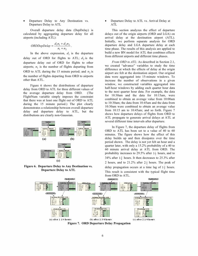
Figure 6 shows the distributions of departure delay from ORD to ATL for three different values of the average departure delay from ORD. (The FlightNum variable simply imposes the constraint that there was at least one flight out of ORD to ATL during the 15 minute period.) The plot clearly demonstrates a relationship between overall departure delay and departure delay to ATL, but the distributions are clearly non-Gaussian.

(a) (b)

(c)

Figure 6. Departure Delay to Any Destination vs. Departure Delay to ATL

• Departure Delay to ATL vs. Arrival Delay at ATL

This section analyzes the effect of departure delays out of the origin airports (ORD and LGA) on arrival delay at the destination airport (ATL). Initially, we perform separate analysis for ORD departure delay and LGA departure delay at each time phase. The results of this analysis are applied to build a new BN model for ATL that combines effects from different airports and different time phases.

From ORD to ATL: As described in Section 2.1, we created “advance” variables to study the time difference at which the effects of delay at the origin airport are felt at the destination airport. Our original data were aggregated into 15-minute windows. To increase the number of observations in a given window, we constructed variables aggregated into half-hour windows by adding each quarter hour data to the next quarter hour data. For example, the data for 10:30am and the data for 10:15am, were combined to obtain an average value from 10:00am to 10:30am; the data from 10:45am and the data from 10:30am were combined to obtain an average value from 10:15 am to 10:45am; and so forth. Figure 7 shows how departure delays of flights from ORD to ATL propagate to generate arrival delays at ATL at several different time intervals after departure.

In Figure 7, the departure delay of flights from ORD to ATL has been set to a value of 40 to 60 minutes. The figure shows how the effect of this delay builds up and then dissipates over the time period shown. The delay is not yet felt an hour and a quarter later, with only a 15.2% probability of a 40 to 60 minute arrival delay at ATL from ORD. The probability increases to 29.5% after 1 1

2 hours, and to

34% after 1 34

hours. It then decreases to 25.3% after 2 hours, and to 21.2% after 2 1

4 hours. The peak of

delay propagation occurs at a time lag of 1 34

hours. This result is consistent with the typical flight time from ORD to ATL.

Figure 7. ORD Departure Delay Propagation

7

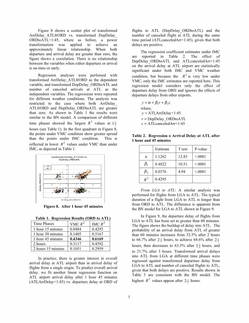
Figure 8 shows a scatter plot of transformed

ArrDelay_ATLfrORD vs. transformed DepDelay_ ORDtoATL+1:45, where as before, a power transformation was applied to achieve an approximately linear relationship. When both departure and arrival delay are greater than zero, the figure shows a correlation. There is no relationship between the variables when either departure or arrival is on-time or early.

Regression analyses were perfomed with transformed ArrDelay_ATLfrORD as the dependent variable, and transformed DepDelay_ORDtoATL and number of canceled arrivals at ATL as the independent variables. The regressions were repeated for different weather conditions. The analysis was restricted to the case where both ArrDelay_ ATLfrORD and DepDelay_ORDtoATL are greater than zero. As shown in Table 1 the results were similar to the BN model. A comparison of different time phases showed the largest 2

R values at 1 34

hours (see Table 1). In the first quadrant in Figure 8, the points under VMC condition show greater spread than the points under IMC condition. This is reflected in lower 2

R values under VMC than under IMC, as depicted in Table 1.

Figure 8. After 1 hour 45 minutes

Table 1. Regression Results (ORD to ATL) Time Phases VMC 2

R IMC 2R

1 hour 15 minutes 0.0484 0.4293 1 hour 30 minutes 0.1405 0.5167 1 hour 45 minutes 0.4346 0.6169 2 hours 0.3117 0.4592 2 hours 15 minutes 0.1051 0.2959

In practice, there is greater interest in overall

arrival delay at ATL airport than in arrival delay of flights from a single origin. To predict overall arrival delay, we fit another linear regression function on ATL airport arrival delay after 1 hour 45 minutes (ATLArrDelay+1:45) vs. departure delay at ORD of

flights to ATL (DepDelay_ORDtoATL) and the number of canceled flight at ATL during the same time period (ATLcanceledArr+1:45), given that both delays are positive.

The regression coefficient estimates under IMC are reported in Table 2. The effect of DepDelay_ORDtoATL and ATLcanceledArr+1:45 on the arrival delay at ATL airport are statistically significant under both IMC and VMC weather condition, but because the 2

R is very low under VMC, only the IMC estimates are reported here. This regression model considers only the effect of departure delay from ORD and ignores the effects of departure delays from other airports.

cry21

!!" ++= where,

=y ATLArrDelay+1:45 =r DepDelay_ORDtoATL =c ATLcanceledArr+1:45

Table 2. Regression o Arrival Delay at ATL after 1 hour and 45 minutes

Estimate T test P-value

α 1.1262 12.83 <.0001

1! 0.4822 10.51 <.0001

2! 0.0376 4.94 <.0001 2R 0.4295

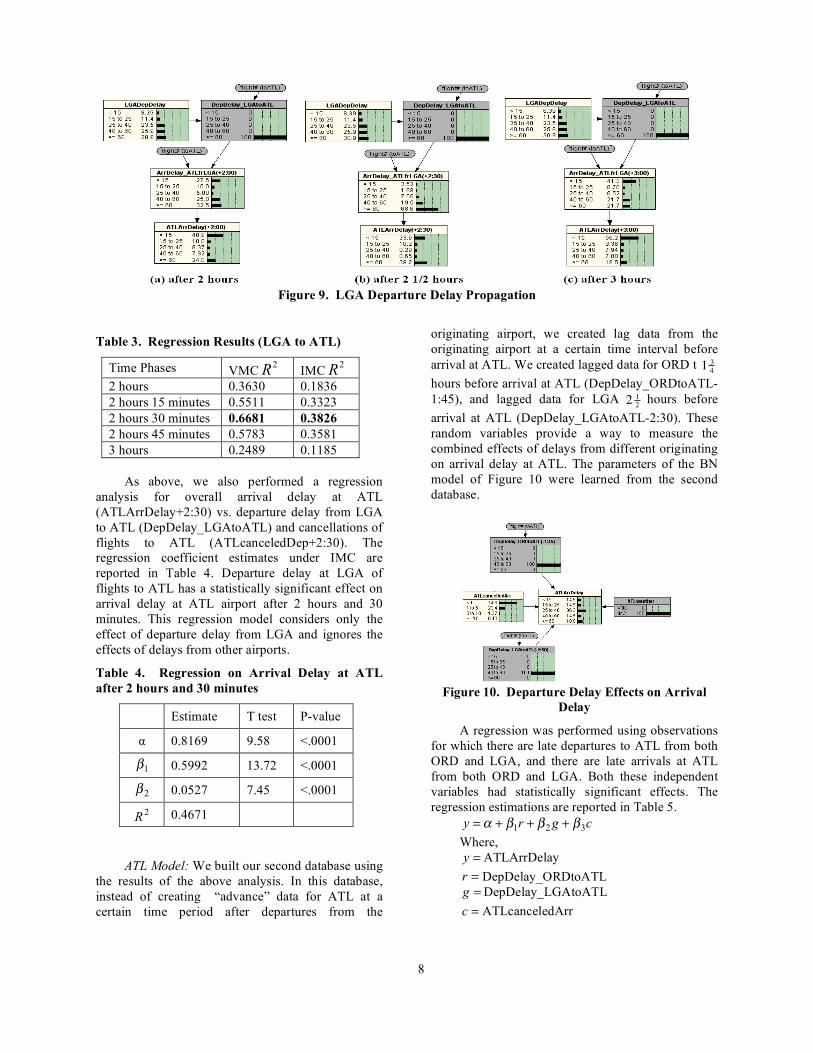
From LGA to ATL: A similar analysis was

performed for flights from LGA to ATL. The typical duration of a flight from LGA to ATL is longer than from ORD to ATL. The difference is apparent from the BN model for LGA to ATL shown in Figure 9.

In Figure 9, the departure delay of flights from LGA to ATL has been set to greater than 60 minutes. The figure shows the buildup of delay into ATL. The probability of an arrival delay from ATL of greater than 60 minutes increases from 32.5% after 2 hours to 66.7% after 2 1

4 hours, to achieve 68.6% after 2 1

2

hours, then decreases to 63.5% after 2 3

4 hours, and

to 21.7% after 3 hours. Transformed arrival delays into ATL from LGA at different time phases were regressed against transformed departure delay from LGA to ATL and number of canceled flights to ATL, given that both delays are positive. Results shown in Table 3 are consistent with the BN model. The highest 2

R values appear after 2 1

2 hours.

8

Figure 9. LGA Departure Delay Propagation

Table 3. Regression Results (LGA to ATL)

Time Phases VMC 2R IMC 2

R 2 hours 0.3630 0.1836 2 hours 15 minutes 0.5511 0.3323 2 hours 30 minutes 0.6681 0.3826 2 hours 45 minutes 0.5783 0.3581 3 hours 0.2489 0.1185

As above, we also performed a regression

analysis for overall arrival delay at ATL (ATLArrDelay+2:30) vs. departure delay from LGA to ATL (DepDelay_LGAtoATL) and cancellations of flights to ATL (ATLcanceledDep+2:30). The regression coefficient estimates under IMC are reported in Table 4. Departure delay at LGA of flights to ATL has a statistically significant effect on arrival delay at ATL airport after 2 hours and 30 minutes. This regression model considers only the effect of departure delay from LGA and ignores the effects of delays from other airports.

Table 4. Regression on Arrival Delay at ATL after 2 hours and 30 minutes

Estimate T test P-value

α 0.8169 9.58 <.0001

1! 0.5992 13.72 <.0001

2! 0.0527 7.45 <.0001 2R 0.4671

ATL Model: We built our second database using

the results of the above analysis. In this database, instead of creating “advance” data for ATL at a certain time period after departures from the

originating airport, we created lag data from the originating airport at a certain time interval before arrival at ATL. We created lagged data for ORD t 1 3

4

hours before arrival at ATL (DepDelay_ORDtoATL-1:45), and lagged data for LGA 2 1

2 hours before

arrival at ATL (DepDelay_LGAtoATL-2:30). These random variables provide a way to measure the combined effects of delays from different originating on arrival delay at ATL. The parameters of the BN model of Figure 10 were learned from the second database.

Figure 10. Departure Delay Effects on Arrival

Delay

A regression was performed using observations for which there are late departures to ATL from both ORD and LGA, and there are late arrivals at ATL from both ORD and LGA. Both these independent variables had statistically significant effects. The regression estimations are reported in Table 5.

cgry321

!!!" +++= Where,

=y ATLArrDelay =r DepDelay_ORDtoATL =g DepDelay_LGAtoATL =c ATLcanceledArr

9

Table 5. Regression Results (ATL)

Estimation T test P-value

α 0.7910 5.18 <.0001

1! 0.4394 4.87 <.0001

2! 0.2260 2.92 0.0051

3! 0.0428 4.69 <.0001 2R 0.7185

Comparing this result to the previous analyses,

the estimated value of arrival delay at ATL (ATLArrDelay) from DepDelay_ORDtoATL and DepDelay_LGAtoATL are more accurate than regressing on either airport alone.

BN Model Validation The BN structure was validated and the

parameters were estimated using 90% of the observations collected between November 2003 and January 2004. The remaining 10% of the observations were withheld to test the model and evaluate its prediction accuracy. The node ATLArrDelay, arrival delay at ATL, in ATL model was chosen for this purpose. During the testing process, the values of ATLArrDelay are treated as unknown. For evaluation, we used Netica’s built-in capability for evaluating the prediction accuracy of a model. The evaluation is conducted by passing through the cases in the data file one by one. For each case, Netica reads in the values of nodes in this row of data, except the value for ATLArrDelay node. A probability distribution is generated for this node based on the values of the other variables in the case and the parameters learned from the 90% training sample. The prediction is then compared with the true value of the node as supplied in the data file. Several different measures of prediction accuracy are available. Our evaluation is based on the confusion matrix, which provides information about the likelihood Netica assigns to each of the discrete bins, conditional on the bin in which the true value lies.

As noted above, we found delay propagation effects only when arrival delays at ATL are positive. We restricted our evaluation to cases in which there was positive overall arrival delay at ATL, and also positive arrival delay at ATL of flights from both ORD and LGA. There are 58 data points in our training set and 21 data points in our testing set that meet these criteria.

The following tables report the confusion matrix for predicting ATL Arrival Delay using

different parameter estimation methods. Bin1 refers to arrival delay less than 15 minutes, Bin2 refers to arrival delay greater or equal to 15 minutes but less than 25 minutes, Bin3 is 25 to 40 minutes, Bin4 is 40 to 60 minutes and Bin5 refers to greater or equal to 60 minutes. Matrix (a) shows results based on a Netica BN model with parameters estimated from the training set using a uniform prior distribution. Matrix (b) shows results based on the linear regression model. Matrix (c) shows results based on the same Netica BN model, but using the linear regression equation as the prior distribution, and updating the CPT by learning from cases. If all incorrect predictions are given equal weight, then the error rate is:

%100#

#!=

"casestotal

casesctedwrongprediErrorRate

Table 6. Confusion Matrix (a): Uniform Prior

Bin1 Bin2 Bin3 Bin4 Bin5 Bin1 0 0 1 0 0 Bin2 0 1 0 0 0 Bin3 1 0 5 0 0 Bin4 1 0 1 2 0 Bin5 3 0 0 1 5 Error rate = 38.1%

Table7. Confusion Matrix (b): Regression Only

Bin1 Bin2 Bin3 Bin4 Bin5 Bin1 1 0 0 0 0 Bin2 0 0 1 0 0 Bin3 1 2 2 1 0 Bin4 2 1 1 0 0 Bin5 0 1 2 1 5 Error rate = 61.9%

Table 8. Confusion Matrix (c): Informative Prior

Bin1 Bin2 Bin3 Bin4 Bin5 Bin1 0 0 1 0 0 Bin2 0 1 0 0 0 Bin3 0 0 6 0 0 Bin4 0 0 1 3 0 Bin5 0 0 2 0 7 Error rate = 19.1%

A comparison of these error rates shows clearly

that our empirical Bayes estimation method outperforms both multinomial learning with a uniform prior distribution and linear regression alone. Interestingly, multinomial learning with a uniform

10

prior distribution performed better than linear regression alone. We suspect this is due to a poor fit of the normal distribution to our data. Although the normal model performed poorly on its own, it provided useful information to develop an informative prior distribution for Bayesian learning.

Conclusions This research demonstrates the utility of

Bayesian networks as a tool for studying how subsystem-level causes propagate to system-level effects. Our models provide a clear demonstration of how delays at an origin airport propagate to create delays at a destination airport. The models can take account of variables such as weather effects and flight cancellations. While the present study considered only a small part of the huge national aviation system, it is clear that the method could be extended to include additional airports. Bayesian networks provide a parsimonious language for representing both the internal behavior of subsystems and the interconnections between subsystems. Thus, Bayesian networks provide a powerful tool for analyzing the interface between micro and macro level phenomena.

Another advantage of Bayesian networks is the ability to provide approximate models for complex, poorly understood problems, especially for parts of the problem with insufficient data for traditional statistical analysis. Previous studies have applied Bayesian networks to aviation systems. In one study, Bayesian networks were used as a demonstration of decision framework. [6] Another study found that the use of Bayesian networks did not provide useful information because of missing data and unmeasured factors.[5] Our study demonstrated that integrating human judgment with statistical analysis in structure construction and parameter estimation can not only save time and effort, but improve prediction accuracy as well.

The software package Netica we used is limited to discrete variables. Some information may be lost in the disretization process. Our empirical Bayes parameter estimation method used linear regression, but our analysis identified situations where linear regression could not be applied, thus limiting the applicability of our technique. There are numbers of aviation databases describing the system performance from different perspective. Many factors which can affect airport delay such as demand, en route weather, aircraft type are not included in our model. We expect that a more complex and sophisticated model based on more complete data could achieve more accurate predictions. Nevertheless, the

approach developed in this paper shows promise as an important new tool for studying how system-level effects arise from subsystem-level causes.

References [1] Hansen,Mark, Tatjana Bolic, June 2001,

Delay and Flight Time Normalization Procedures for Major Airoports: LAX Case Study , UCB_ITS_RR_2001_5, ISSN 0192 4095.

[2] Hansen,Mark, Dale Peterman, 2004, Throughput Effect of Ime_Based Metering at Los Angeles International Airport , Journal of the Transportation Research Board, No.1888, pp.59_65

[3] Nilim, A., Ghaoui, L. E., Hansen, M. and Duong, V., 2001, Trajectory_based Air Traffic Management (TB_ATM) under Weather Uncertainty, ATM 2001, Santa Fe, New Mexico.

[4] Hansen,Mark, 2004, Post_deployment Analysis of Capacity and Delay Impacts of an Airport Enhancement: Case of a New Runway at Detroit , Air Traffic Control Quarterly Abstracts, Vol.12, No.4, pp.2

[5] Wojcik,Len,Josh Pepper, Kristine Mills, June 2003, Predictability and Uncertainty in Air Traffic Flow Management, CAASD, MITER.

[6] Morris, A. Terry, Plesent W. Goode, 2002, The Aeronautical Data Link: Taxonomy, Architectural Analysis, and Optimization, NASA Langley Research Center.

[7] Citrenbaum, Daniel, Robert Juliano, 1999, A Simplified Approach to Baselining Delays and Delay Costs for the National Airspace System (NAS).

[8] Lamon, Ken, 2002, Fewer Air Traffic Delays in the Summer of 2001.

[9] Allan, S. S., J.A.Beesley, J. E. Evans, S. G. Gaddy, 2001, Analysis of Delay Causality at Newark International Airport,, 4th USA/Europe Air Traffic Management R&D Seminar.

[10] http://www.apo.data.faa.gov/faamatsall.HTM [11] Netica user’s guide: http://www.norsys.com/netica.html

[12] Dougherty, J., Kohavi, R., & Sahami, M. (1995). Supervised and unsupervised discretization of continuous features. Proceedings of the Twelfth International Conference on Machine Learning (pp. 194-202). Tahoe City, CA: Morgan Kaufmann

Acknowledgment This work has been supported in part by NSF

under Grants DMI-0002900, DMI-0049062 and IIS-0325074, by NASA Ames Research Center under

11

Grants NAG-2-1565 and NAG-2-1643, by NASA Langley Research Center and NIA under task order NNL04AA07T, by FAA under Grant 00-G-016, and by George Mason University Research Foundation.

Key Words: Bayesian Network (BN), multinomial /

Dirichlet estimation, linear regression, lagged data, delay propagation, Aviation System Performance Metrics (ASPM).

Biographies: Ning Xu is a Ph.D. candidate at George Mason

University. She received her Masters degree in Systems Engineering from George Mason University at 2003.

Dr. George L. Donohue is professor of Systems Engineering and Operations Research at George Mason University. He received his Ph.D. in Mechanical and Aerospace Engineering from Oklahoma State University. From 1994 to 1998 he was Associate Administrator of the Federal Aviation Administration for Research, Engineering and Acquisition. He is director of Center for Air Transportation Systems Research (CATSR) at George Mason University.

Dr. Kathryn Blackmond Laskey is associate professor of Systems Engineering and Operations Research at George Mason University. She received her Ph.D. in Statistics and Public Affairs from Carnegie Mellon University. She is co-director of the Homeland Security and Military Transformation Laboratory at George Mason University.

Dr. Chun-Hung Chen is associate professor of Systems Engineering and Operations Research at George Mason University. He received his Ph.D. in Simulation and Decision from Harvard University.