Estimating the determinants of population location in Auckland

David C. Maré and Andrew Coleman

Motu Working Paper 11-07

Motu Economic and Public Policy Research

May 2011

i

Author contact details David C. Maré Motu Economic and Public Policy Research and the University of Waikato Dave.Mare@motu.org.nz Andrew Coleman Motu Economic and Public Policy Research Andrew.Coleman@motu.org.nz Acknowledgements We extend our thanks to Arthur Grimes for helpful discussions on various aspects of our work, to Mairéad de Roiste and Andrew Rae of Victoria University for assistance with GIS manipulation, and to EeMun Chen, from the Auckland Policy Office (MED), for constructive discussions. Thanks also to the helpful comments of two anonymous referees. Access to Census data, and to the employment location data used in this study, was provided by Statistics New Zealand under conditions designed to give effect to the security and confidentiality provisions of the Statistics Act 1975. All non-regression results using Census data are subject to base three rounding in accordance with Statistics New Zealand’s release policy for Census data. Information on the location of employment is drawn from Statistics New Zealand’s prototype Longitudinal Business Database. Only people authorised by the Statistics Act 1975 are allowed to see data about a particular business or organisation. The results in this paper have been confidentialised to protect individual businesses from identification. The results are based in part on tax data supplied by Inland Revenue to Statistics NZ under the Tax Administration Act 1994. This tax data must be used only for statistical purposes, and no individual information is published or disclosed in any other form, or provided back to Inland Revenue for administrative or regulatory purposes. Any person who had access to the unit-record data has certified that they have been shown, have read and have understood section 81 of the Tax Administration Act 1994, which relates to privacy and confidentiality. Any discussion of data limitations or weaknesses is not related to the data's ability to support Inland Revenue's core operational requirements. Any table or other material in this report may be reproduced and published without further licence, provided that it does not purport to be published under government authority and that acknowledgement is made of this source. The opinions, findings, recommendations and conclusions expressed in this report are those of the authors. Statistics New Zealand, the Ministry of Economic Development, the Ministry of Transport, the Ministry for the Environment, the Department of Labour, Motu and the University of Waikato take no responsibility for any omissions or errors in the information contained here. The paper is presented not as policy, but with a view to inform and stimulate wider debate. This paper has been prepared with funding from the Ministry of Science and Innovation’s Cross Departmental Research Pool fund secured and administered by the Ministry of Economic Development, New Zealand Government – Auckland Policy Office. Motu Economic and Public Policy Research PO Box 24390 Wellington New Zealand Email info@motu.org.nz Telephone +64-4-939-4250 Website www.motu.org.nz © 2011 Motu Economic and Public Policy Research Trust and the authors. Short extracts, not exceeding two paragraphs, may be quoted provided clear attribution is given. Motu Working Papers are research materials circulated by their authors for purposes of information and discussion. They have not necessarily undergone formal peer review or editorial treatment. ISSN 1176-2667 (Print), ISSN 1177-9047 (Online).

ii

Abstract This paper analyses the location choices of new entrants to Auckland between 1996 and 2006, to identify a systematic relationship between residential location choices and features of local areas such as population density, the population composition of the area or its neighbourhood, accessibility to different types of amenities, paying particular attention to the influence of land prices. For the analysis, the Auckland Urban Area is divided into around 9,000 small areas (“meshblocks”). Location choices are analysed using count data methods applied to microdata from the Census of Population and Dwellings. The results emphasise the importance of own-group attraction. Groups of entrants classified by qualification, income, ethnicity, or country of birth are all attracted to meshblocks or neighbourhoods where their group already has a strong presence. The evidence demonstrates that this sorting reflects attraction to fellow group members, rather than being due to group members having common preferences for local amenities.

JEL codes R12 – Size and Spatial Distributions of Regional Economic Activity; R23 – Regional Migration; Regional Labor Markets; Population; Neighborhood Characteristics; R31 – Housing Supply and Markets Keywords Auckland; residential location choice; count data models

iii

Contents

1 Introduction ................................................................................................................... 1

2 Modelling location choice ............................................................................................ 3 2.1 Review of prior literature .................................................................................... 4 2.2 Theory and empirical specification ................................................................... 9

2.2.1 Estimation .......................................................................................... 16 2.3 Identification issues ........................................................................................... 17

3 Data 22 3.1 Population location - Census of Population and Dwellings ........................ 23 3.2 QVNZ land values ............................................................................................. 24 3.3 Amenity data ....................................................................................................... 25 3.4 Population composition .................................................................................... 26

4 Results ........................................................................................................................... 26 4.1 Area characteristics – data description ........................................................... 27 4.2 Valuation of amenities ....................................................................................... 29 4.3 Patterns of inflows ............................................................................................. 33 4.4 Location choice regressions ............................................................................. 35

4.4.1 Treating amenities as unobserved .................................................. 35 4.4.2 Including observed amenity measures ........................................... 39

5 Discussion..................................................................................................................... 42 5.1 Main findings ...................................................................................................... 44

References .............................................................................................................................. 46

Tables

Table 1: Summary statistics – area characteristics ......................................................... 50

Table 2: Local Population Characteristics (2006) ......................................................... 51

Table 3: Land-price regressions ....................................................................................... 52

Table 4: Profiles of entrant subgroups (2006) ............................................................... 54

Table 5: Location choice ................................................................................................... 55

Table 6: Location choice – by ethnicity .......................................................................... 56

Table 7: Location choice – by country of birth ............................................................. 57

Table 8: Location choice (with amenities) ..................................................................... 58

Table 9: Location choice (with amenities): by ethnicity ............................................... 60

Table 10: Location choice (with amenities): by country of birth .................................. 62

Table 11: Interpretation of own-group effects ................................................................ 65

Figures

Figure 1 Location choice and income ............................................................................. 66

1

1 Introduction

Big cities offer their citizens a myriad of places to live. Households can choose to

live near the central city, near their workplace, near nice views or convenient amenities, in

places with good transport facilities, near other people with similar characteristics to

themselves (such as age, education, or ethnicity), or simply where it is cheap. Households

typically consider a variety of locations when choosing where to live, choosing the place that

provides the best value for money as their circumstances permit. These choices not only

determine aggregate location patterns for groups of people who share common

characteristics, but also determine the price of land in each location.

This paper analyses the location patterns of new entrants to Auckland between

1996 and 2006. During this period, approximately 300,000 people migrated to Auckland,

helping increase the overall population from 998,000 to 1,208,000. While many of these

people came from other parts of New Zealand, a large number came from overseas,

particularly the United Kingdom, Asia, Australia, and the Pacific Islands, and some were

New Zealanders returning to Auckland after living abroad. This paper uses statistical

techniques to examine the characteristics of places where these new residents chose to live. It

does this by ascertaining whether there is a systematic relationship between residential

location choices and features of local areas such as population density, the population

composition of the area or its neighbourhood, accessibility to different types of amenities,

and the price of land. For the analysis, the city is divided into around 9,000 small areas

(“meshblocks”).

The patterns of land prices and residential location choices are of potential interest

for several reasons. For example, city planners need to know the best places to build new

amenities, roads, or public transport infrastructure, government officials are interested in the

causes and potential adverse effects of income-based clustering, and urban economists are

interested in the extent to which idiosyncratic preferences rather than income determine

location patterns. This paper is intended to shed light on all three topics. It analyses the

willingness of different population groups to locate near different physical amenities. It

analyses the extent to which people with certain characteristics like to cluster close together,

or how they avoid other groups. And it attempts to estimate the extent to which location

choices by different groups of people reflect their different valuation of amenities, not just

their different ability to pay.

2

The paper focuses on the location patterns of new entrants to Auckland rather than

existing residents, for two main reasons. First, the resultant location patterns will be of

interest to city planners if Auckland’s future population growth is driven by net entry. The

paper shows that the location patterns of Pacific Island migrants, Chinese migrants, and New

Zealanders returning from overseas are quite different; if the city planners are able to predict

the types of entrants most likely to arrive in Auckland in the future, they will be better able to

anticipate the needs for facilities in places where these people are most likely to want to live.

The paper also offers insights on the relative importance of different amenities to different

groups of people, and their willingness to pay for them. Secondly, the location patterns of

existing residents may not be determined by current prices and amenities, as they reflect

decisions made at an earlier time. If it is expensive to buy and sell real estate, or it is

expensive to disrupt long-term arrangements to obtain local services such as schooling, a

household may be living in a place even though it is no longer their best choice and they

would move if it were not so costly.

The econometric approach is not straightforward, because the price of land in each

location depends on many factors, several of which are unobserved. The essential difficulty is

that areas that are highly priced are usually highly priced because of their convenience to

desirable amenities, or because of characteristics of the people living in the region;

consequently, they are also in high demand despite their high prices. If some of these

amenities are unmeasured, it will appear that the demand to live in a particular location is

increasing rather than decreasing with price. The econometric techniques we use attempt to

adjust for these unobserved factors in order to estimate how different groups value various

amenities. To our knowledge, this is the first attempt to estimate how population location

patterns are simultaneously affected by price and amenity location for any major city. For this

reason, the paper contains an extensive discussion of our procedures.

Our overall findings confirm the patterns identified in a companion paper (Maré et

al, 2011), which highlighted the importance of residential sorting along social lines. The

added insight from the current paper is that the patterns of sorting cannot be accounted for by

group-level differences in preferences for observed amenities or by land price-based

stratification. We show that greater accessibility to the amenities that we examine is

associated with higher land prices, confirming increased willingness to pay for more

desirable locations. However, with the exception of access to the Central Business District

(CBD), locations with convenient access to amenities do not attract greater total inflows of

3

entrants, possibly because the desirability of the areas is balanced by the consequently higher

land prices. Instead, entrants to Auckland are strongly attracted to areas where the existing

population has characteristics similar to their own, even controlling for the influence of

amenities and land prices. The flow of entrants into the Auckland Urban Area thus reinforces

existing subgroup concentrations. Residents born in South Korea, for example, account for

two percent of the Auckland Urban Area population, yet the average South Korean lives in a

meshblock where nine percent of the population is from South Korea. Our results suggest

that, conditioning on prices and amenities, South Korean-born entrants are three times more

likely to choose a meshblock in which South Korean-born residents are already concentrated

than in a meshblock with an average share (2%) of South Korean-born residents. Similarly

strong sorting is observed for other recent migrant groups from Asian and Pacific countries.

There is also significant, though somewhat less pronounced, sorting of groups defined by

qualification level and ethnicity.

2 Modelling location choice

The starting point for this paper is the observation that observed location choices

within Auckland vary markedly across population subgroups. In a companion paper (Maré et

al, 2011), we have documented substantial residential segregation, which is particularly

pronounced on the basis of ethnicity, region of birth, qualification and income. These

findings confirm and extend previous findings by Johnston et al. (2010), which focused on

segregation by ethnicity.

The current paper extends the previous analysis by analysing possible reasons for

the observed segregation patterns. Specifically, we investigate the extent to which the

observed patterns can be accounted for by groups being differentially attracted to particular

locational amenities. If that were the case, local government policies to influence access to

local goods, services and facilities will affect the population mix in an area. Heterogeneous

demand for access to different amenities will also influence the extent to which accessibility

is translated into higher land prices, as opposed to higher population density.

There is a well-established literature on the causes and consequences of residential

segregation; much of it is focused on racial segregation patterns in the United States. Studies

document the role of discrimination in the US context (Massey, 2008), but also examine the

potential for segregation to arise as a consequence of different groups benefiting from

4

different local amenities or population mixes (Schelling, 1969; Tiebout, 1956; Cutler and

Glaeser, 1997).

By identifying the influence of local amenities on residential location choices in

Auckland, we hope to be able to explain some of the segregation patterns, and delineate the

scope for local policies to influence Auckland’s evolving urban form through influencing the

provision of local amenities. Any segregation that remains after we have controlled for

differential attraction to amenities could reflect either preferences for locating among fellow

group members (or away from non-group-members), ordiscrimination. In either case, there

may be multiple equilibria – we can expect to observe clustering, but will be unable to predict

where in Auckland the clustering will occur.

2.1 Review of prior literature

The economic literature analysing residential location decisions has two main

strands. The first of these analyses the factors that induce people to live in one city rather than

another. Following Roback (1982), this literature assumes people choose where to live based

on a combination of earnings potential, the cost of living, and the amenities available in each

city. It assumes people migrate until they are indifferent between locations; and that this

generates an equilibrium system of cities broadly characterised by population size, wages,

and land prices. The effect of amenities on these three factors is complex, depending on

whether amenities are valued by firms as well as residents. A city with amenities that are

useful to firms but unattractive to residents will tend to have high wages and low land prices.

A city with amenities that are attractive to residents will tend to have high land prices, but

will offer relatively low wages unless firms value these amenities sufficiently to compensate

for the high land prices they must pay. Subsequent refinements have analysed how land rents,

population size, and wages depend on the structure of taxes, the cost of developing land and

building houses, and the relative value of amenities to residents, to firms producing tradeable

goods, and to firms producing non-tradeable goods (Albouy, 2009; Glaeser and Gottlieb,

2009). The primary analytical insight is that population densities and land values are

simultaneously determined by the way people move between cities in response to locational

amenities.

Empirical research has confirmed some of the predictions of this literature, even if

the basic assumption – that people migrate until they are indifferent between locations –

remains difficult to verify. In the United States, for example, the desirability of coastal

5

locations and of pleasant winter conditions has been rigorously established, and it has been

demonstrated that favourable amenities tend to be priced into high rents rather than low

wages, but unfavourable amenities are reflected in both high wages and low rents (Rappaport,

2008). This literature has shown that the effect of amenities on land values and population

density reflects the simultaneous and complex interaction of multiple factors. In the south of

the United States, for example, low construction costs have meant house prices have been

little affected by the large inward migrations that have occurred in response to a favourable

winter climate (Glaeser and Gottlieb, 2009). Other work has shown that other attractive

amenities include good educational facilities, good transport infrastructure, and low crime

(Gottlieb, 1994; Florida, 2000; Duranton and Turner, 2008).

The second strand of the literature has analysed where people locate within a city.

A major difference between the between-city and within-city analysis is that within a city

people face essentially the same wage distribution, but that the transport costs associated with

commuting to work and accessing different amenities differ according the location within the

city. A major theme of this literature has concerned the relationship between population

density and land prices across parts of the city that differ in terms of their convenience to

attractive amenities including employment opportunities. Attempts to estimate the extent to

which different amenities are incorporated into land prices have generally proved difficult,

for several reasons. One problem is simultaneity: valued amenities tend to attract wealthier

households, who in turn attract other amenities (such as better quality service industries) that

further enhance the desirability of the neighbourhood. Since the quality of services is

generally poorly measured in the available datasets, it can be very difficult to isolate the

effect of individual amenities on prices. The problem is compounded if the average wealth or

income of the local population is considered a desirable feature of the location in its own

right. A second problem is that many of the amenities are unobserved by the econometrician.

This induces a bias into the estimates of how prices affect location patterns, for people are

attracted to highly priced places, not because they highly priced but because there are

attractive amenities. Both of these problems induce spatial correlation into the estimation

procedure, further complicating the analysis.

A second theme has been the extent to which people tend to locate in clusters near

people who are similar to themselves. Empirically, spatial clustering proves to be very

important, although it proves difficult to be precise as to why it occurs (Nechyba and Walsh,

2004, p. 183). The literature has identified three major reasons why clustering happens: it can

6

occur because people have preferences as to the characteristics of their neighbours, such as

their age, race or income; it can occur because people of a particular type have preferences

over the quality of certain local services such as schools that are affected by the

characteristics of the people living in the local neighbourhood; and thirdly it can happen

because people have preferences over the quantity of amenities funded by local taxes, and

they move to areas composed of people with similar preferences and incomes. The latter

factor is likely to be relatively unimportant in New Zealand, given the structure of city level

funding. Nonetheless, ethnicity-based clustering is a significant feature of Auckland’s spatial

population distribution (Johnston et al, 2010; Maré et al, 2011).

One aspect of spatial clustering is the tendency of migrants to a city to locate in

neighbourhoods with people of similar ethnicity or background. This clustering can occur for

both positive and negative reasons: new migrants may wish to live with people they know, or

in an area that is culturally familiar; or new migrants may be prevented from going to other

areas, either because they are discriminated against or because they cannot afford more

expensive neighbourhoods (Cutler et al, 1999). These reasons have different effects on land

rents, however. For example, if migrants strongly desire to live in areas with people from the

same ethnic group, they will pay a premium to live in these areas compared to other areas

with similar amenities; if large numbers of other people “flee” areas dominated by a

particular ethnic group, rents will be relatively low. Cutler, Glaeser, and Vigdor (1999)

showed that rural blacks migrating to urban locations in the United States had three different

urban migration experiences during the twentieth century, including a period when migrating

blacks paid a premium to live in areas with a large black population.

The empirical literatures examining how amenities affect between-region and

within-region price and migration patterns have proceeded quite differently. The between-

region literature has tended to focus on geographic or historic differences, so that causal

identification is possible. (See, for example, Rappaport (2008) on the effects of physical

geography, or Baum-Snow (2007) or Duranton and Turner (2008) on the effect of historic

highway developments.) With some exceptions such as Black (1999), who used school

district lines to analyse how school quality affected residential land prices, it has proved

much more difficult to identify the effect of different amenities in the within-region literature.

Rather, the literature has largely followed one of three approaches. One approach has

estimated hedonic price equations to find out the reduced form relationship between

amenities or population characteristics, and land prices. A second approach has estimated the

7

importance of different amenities or population characteristics in determining where people

choose to live, although typically without reference to prices. A third approach has estimated

how transport infrastructure, distance, and transport costs jointly affect prices and location

patterns.

While hedonic price equations have been used by various authors to estimate how

different characteristics of houses affect property prices, it has proved far from

straightforward to consistently estimate the effect of different locational amenities on prices.

In large part, this is due to the difficulties of unobserved amenity quality (Sheppard, 1999).

People value being conveniently located to a large number of different amenities, most of

which cannot be included in statistical analysis; as there is a positive correlation between the

quality of many amenities in an area, estimates of the value of any particular amenity are

likely to biased. In the absence of a well-targeted identification strategy for estimating the

effect on prices of a particular characteristic, spatial hedonic price equations typically

produce biased estimates of the underlying structural relationships.

Since the 1970s, there have been numerous studies adopting the second approach of

analysing where firms or households choose to locate. Many of these have used the random

utility model pioneered by McFadden (1978) and, following Carlton (1983), have focused on

the decisions of new firms or households entering an area. In general, the literature has been

more successful in determining where different groups of entrants locate than determining

why they locate in these regions, as it has proved challenging to unpick the extent to which

migrating firms of residents are attracted or repelled by particular amenities, and the extent to

which they are prepared to pay the price for these amenities. As this problem is the focus of

our paper, the issue is discussed at length in sections 2.2 and 2.3 below.

The most successful empirical literature is that which has has taken the third

approach and has analysed how transport costs jointly affect prices and location patterns. The

literature began by estimating a land price bid-rent gradient as a function of the distance to

the central city. The basic argument, developed by Alonso (1964), Mills (1967), and Muth

(1969), is that if people work or play in the central city, they will pay a premium for land

located close to the centre to reduce their commuting costs. Moreover, if transport to the

centre is particularly cheap in certain locations, possibly because of public transport or a

highway, these locations should also have relatively high land prices. If the demand for land

is a rising function of income and a declining function of its price, land prices and density

8

should both be a declining function of the distance from the centre. For this reason, older

cities are often characterised by densely populated corridors around transport networks

(LeRoy and Sonstelie, 1983; Frost, 1991).

While most empirical evidence suggests population density declines with distance,

Anas, Arnott, and Small (1998) argue that most cities have prominent subcentres that account

for a large share of employment. These subcentres temper the relationship between land

prices and distance to the central city. Since commuting to work and various social, shopping,

and recreational amenities is expensive, and since households have limited incomes, this

argument suggests conveniently-located land will trade at a premium wherever it may be

located, even if this is not close to the city centre. The decentralised nature of modern cities,

including Auckland, is now well established in the literature, particularly as the widespread

use of the motor car for work-place commuting has meant most people can live 15–30 miles

from a workplace and still commute within 30 minutes (Baum-Snow, 2007; Glaeser and

Kohlhase, 2004; Moses and Williamson, 1967). While the most convincing evidence of the

causal effect of transport infrastructure investment on residential location patterns comes

from historic studies of highway development (Baum-Snow, 2007), many studies have

established a correlation between local land prices, population density, and access to transport

facilities.

A fourth approach to investigating residential location choices is to analyse

subjective reports of what people value about living in particular areas. A recent study

collected such information from a sample of 20–40 year old movers in Auckland (Saville-

Smith and James, 2010). When asked about their criteria for selecting a house, the most

prevalent responses related to having more space (a larger house as well as a larger section)

and lower financial cost. Recent movers reported seeking improvements in access to

education, employment, and family, and reductions in transport costs, though the study did

not identify to which amenities the desired transport provided access. The study also

identified a range of tradeoffs that movers made between criteria.1 Studies such as this are

valuable in identifying criteria and trade-offs, but in order to build a broader picture of the

terms of the trade-offs, as revealed by people’s actual choices, we rely on modelling of

patterns of revealed preferences.

1 Relevant findings are covered in Tables 10.1 and 10.2, and section 10.3.

9

2.2 Theory and empirical specification

People entering Auckland choose where to live based on a trade-off between the

costs and benefits of different dwellings. When choosing a dwelling, a person simultaneously

chooses a house, an associated quantity of land, and a location, for which they either pay an

implicit or explicit rent. For this rent, the person obtains private use of the dwelling and its

land, and also gains access to a range of amenities. The costs of this access depend on the

location of the property, and reflect the ease of access to each amenity. The net (after

transport cost) income that the person can earn will also depend on their residential location

due to location-varying costs of access to employment. The person is assumed to choose a

dwelling that offers the best combination of housing, land quantity, convenience, and

affordability, the last defined in terms of the ability to consume other goods and services.

Before formalising this trade-off in terms of utility maximisation, it is important to

clarify what is meant by the term “rent.” In general, properties can either be purchased

outright, at a price P, or leased for a monthly or annual rent. Conceptually, we wish to use

“rent-equivalent,” which is equal to the annual rent if the property is leased, or the implicit

annual opportunity cost if the property is owned. The annual opportunity cost can be thought

of as the annual rent a landlord would need to charge if they were to cover their costs: this

includes the real interest cost (the real interest rate multiplied by the price of the property),

rates, and maintenance. This “rent-equivalent” can be split into a “building-rent” component

θ covering the costs associated with providing the property’s buildings and a “land-rent”

component r covering the costs associated with providing the land. The focus of this paper is

the implicit land rent, which is the cost of obtaining space in a particular location. In

equilibrium the location-specific per unit land rent includes a capitalisation of the advantages

of locating in that place, as valued by the highest bidder.2 We use, as a proxy for land rent,

the price per hectare of land, using land valuation data.

In the following model of location choice an individual i chooses a location x that

maximises her utility, subject to a budget constraint. The utility that i gains in period t from

locating at x is a function of her consumption of consumer goods Cit, her use of land Lit, her

use of housing Hit and her use of locational amenities Ait. Ait is a vector measuring the number

of times each amenity in the city is used by the individual. Note that an amenity need not be

located at x for the individual to use it; rather the location x affects how costly it is to access

2 If there is some consumer surplus, the rent will be only slightly above the second highest bidder’s valuation.

10

the amenity. For convenience it is assumed that choices over the amount of housing and the

amount of land at a location x can be made independently.

Assuming each person i supplies a fixed amount of labour and earns a return on her

human capital of yit , the utility maximisation problem can be considered in three stages. First,

conditional on choosing a location x, person i chooses the quantity of consumption, the house

size, the number of trips to different amenities, and the land size that maximises the utility

function:

,( , , )it i it it it itU f C H A L

subject to a budget constraint:

(1 )it t it xt it xt it it itC H A r L y

The price of consumer goods is assumed to be independent of location and is used

as the numeraire. The housing price θt is also assumed to be independent of location,

although the price of land (rxt) and the cost of accessing amenities (αxt) are location specific.

The costs of travel to work (τxt) are location-specific, and are reflected in the budget

constraint as proportional to yit. Each agent is assumed to treat the prices as exogenously

determined.

Assuming a constant returns Cobb-Douglas log utility function, Uit can be

expressed as:

ln( ) ln( ) ln( ) (1 ) ln( )it i it i it i it i i i itU a C b A h H a b h L (1)

Solving this optimisation problem at a particular location x yields the following

first order conditions, and an indirect utility function indicating the maximum possible utility

available at the location:

* (1 )it i it xtC a y

* (1 )iit it xt

i

hH y

* (1 )iit it xt

i

bA y

* (1 )(1 )i i i

it it xtxt

a b hL y

r

11

* * * * *( ; , ) ( , , , | , , , , )

ln( ) ln( ) ln( ) (1 ) ln( )

( , , , , )

i it it it it it it t xt xt it xt

i it xt i t i xt i i i xt

i it t xt xt xt

U y x t U C H A L r y

y h b a b h r

v y r

(2)

κi is a constant reflecting the individual-specific parameters of the utility function:

ln( ) ln( ) ln( ) (1 ) ln(1 )i i i i i i i i i i i i ih h a a b b a b h a b h

The second stage of the optimisation problem is for the individual to choose the

location x* that maximises utility:

* arg max ( , , , , )it i it t xt xt xtx

x v y r (3)

In practice, the city is divided into a large number M of discrete locations

(meshblocks). For mathematical convenience, x* is best expressed as an M*1 vector with a

“1” in the meshblock that is the optimal choice. This choice will represent the best trade-off

between the convenience of a location and the amount of consumption that can be undertaken

there, that latter measured in terms of consumption goods, housing, and private land use.

The third stage of the optimisation problem concerns the way total demand is

aggregated. For most goods and services, it would be possible to simply aggregate individual

demand to specify a set of demand equations linking the quantity of goods demanded to the

price of those goods; these equations could be used to estimate the basic preference

parameters or demand elasticities. For land markets, however, this approach is problematic,

as land markets are an example of a market with heterogeneous quality. As Rosen (1974)

famously pointed out, an equilibrium in a market characterised by the heterogeneous quality

of the objects for sale operates quite differently than a market where the objects are of

uniform quality. In heterogeneous quality markets, an equilibrium comprises a set of prices

such that for each different quality the number of units demanded is equal to the number

supplied, no households have an incentive to demand a different quality object, and no

supplier can make additional profits by changing the quality of what they produce.

In heterogeneous property markets, prices in different locations find a level that

ensures that the number of properties demanded in each location is equal to the number of

houses available. Prices will be high in areas that offer convenient access to attractive

amenities, to ration the demand for these areas to the available supply, while prices in areas

that are inconvenient (or near unattractive amenities such as rubbish dumps) will be

12

sufficiently low that people will be induced to live in these areas despite the inconvenience.

In the long term, new properties will be developed in the regions where the prices are high

compared to the costs of construction. If it is very expensive to build new houses in high-

priced areas conveniently located to good amenities, perhaps because new construction

involves multi-storied buildings, few new properties will be developed in these locations.

Conversely, many new properties may be developed in relatively low-priced and

inconveniently located areas if construction costs are relatively low in these areas. For this

reason, it is possible for a majority of new houses to be constructed in areas that are not

particularly attractive or convenient, and for a majority of new residents to choose to live in

these innately inconvenient or unattractive places. The fact that people choose to live in a

place does not mean it is attractive, or convenient to valued amenities; rather it means that at

that price, it offers good value compared to other locations.

Econometric equations estimating the factors that determine where people live

need to take these pricing issues into account. If the primary interest is to determine the

location patterns of the total population, equation 3 is aggregated across all individuals to

show demand patterns. Let [ ],[ ],[ ]r be the vectors of prices at the various locations [x],

and Pop the population of the city. The demand for locating at x is

*( ;[ ],[ ],[ ] | ) arg max( ( , , , , ))Pop Pop

t t t Pop it i it t xt xt xtxi i

D x r x v y r

(4)

It is not useful to estimate how the number of households living in each location

depends on the cost of accessing different amenities or on prices, however. This is because in

equilibrium the total demand must equal the number of properties in the location, Sx:

( ) ( ;[ ],[ ],[ ] | )t t t t PopS x D x r (5)

For this equilibrium to occur, land rents must adjust to equate demand with the

available supply. Consequently, a more appropriate specification is an hedonic rent equation,

which captures how land rents vary with the supply of properties and their convenience to

desirable locations:

( ) ( ( ),[ ],[ ] | )

( )

t t t t Pop

popt

r x P S x

r x

(6)

It is possible to estimate a version of equation 4 for population subgroups,

however. Consider a population subgroup Ωg. Then the location demand patterns of this

subgroup are given by

13

*( ;[ ],[ ],[ ] | ) arg max( ( , , , , ))g g

t t t g it i it t xt xt xtxi i

D x r x v y r

(7)

This equation shows the extent to which members of this subgroup are prepared to

trade off the convenience of a location against its price. Since the equation depends on the

characteristics of the subgroup, including its income and preferences, the equation shows how

these characteristics determine the subgroup’s location patterns for a given set of convenience

prices [ ],[ ] and land rents [ ]r . When this equation is evaluated at the equilibrium prices

poptr , it shows the extent to which the population subgroup’s characteristics determine its

actual location patterns. For instance, if a subgroup has low income, it may tend to locate in

inexpensive areas that are relatively inaccessible to desirable amenities, as these areas allow

the best trade-off between convenience and consumption of other goods relative to the

population as a whole. Alternatively, if members of a subgroup desire to locate near a

particular amenity more strongly than other people (which in the log utility model would be

indicated by a particularly high value of one of the parameters ai), this would be reflected by

high demand to live in that area, given equilibrium prices.

Suppose that a location’s access to amenities can be ranked and represented by a

single measure of amenity quality ω. If the meshblock locations are ranked by quality, the

demand for housing by a population subgroup can be represented as a scatterplot of points on

a three dimensional graph that has quality, price, and quantity axes. The points indicate the

quality of the location, the equilibrium price of land at that location, and the number of

residents living at that location. For any group of similar people, the graph should have the

following characteristics (see Figure 1):

a) The points trace out a line indicating the number of residents living in each quality-

specific location at the market price for that quality.

b) When the line is projected into price-quality space, it traces out the market equilibrium

prices for each quality. This is the same for each group. The line should be increasing and

convex: i.e., better quality houses sell for increasingly higher prices.

c) The line lies on a two dimensional surface (not shown in Figure 1) indicating the group’s

willingness to pay for each level of quality. The surface should be increasing in quality

and decreasing in price: that is, for any price, there should be an increasing number of

people wishing to live in houses of better quality, and for any level of quality there should

be a decreasing number of people willing to live in a house as the price rises. The contour

14

of the surface is different for different subgroups. For instance, low-income groups are

likely to be more price-sensitive than high-income groups, yielding a more steeply

negative slope.

d) When the line is projected into price-quantity space, it traces out the number of people

from the group who live in different-priced locations. This line could rise or fall with

prices, and reflects the group’s willingness to pay for quality compared to the market

price for quality. For instance, a high-income group is likely to have the number of

houses rising with price over most of the price range. High-income people don’t want to

live in low-quality areas, despite the low prices: they are prepared to pay more to live in

high-quality areas. Conversely, low-income people are likely to have the number of

houses decline with price: while they are prepared to pay more to live in better areas, their

willingness and ability to pay to live in these areas increases less quickly than the market

price, so they are less likely to be found in high-priced areas. In price-quantity space, the

line of a middle-income group is likely to first increase in price and then decrease in

price. From a position in the middle, middle-income people are not prepared to “trade

down”, for the extra money they would obtain from moving to a lower quality area does

not compensate them for the inconvenience of that area; and while they would like to

“trade up,” they do not because the cost of moving to the higher quality area is too high.

e) When the line is projected into quality-quantity space, it traces out the number of people

from the group who live in different-quality locations. Because prices are increasing in

the quality of locations, this projection has similar characteristics to the projection in

price-quantity space: it shows the willingness of different groups to live in different-

quality locations relative to the market as a whole. Again, a low-income group will be

characterised by having smaller numbers of people in high-quality areas (for even though

low-income people are prepared to pay higher amounts to live in better areas, the amount

they are willing to pay increases less quickly than the market price), while a high-income

group will typically be characterised by having more people living in high-quality areas

than in low-quality areas.

In principle, equation 7 can be used to estimate how a subgroup’s demand to live in

different places depends on land rents and the cost of accessing different amenities in these

locations, and this information can be used to derive information about the group’s

preferences over amenities, land, and consumption goods. To do this properly, location

choices must be expressed as a function of both land prices and amenity costs, so that the

15

willingness to spend on amenities can be calculated. Nonetheless, it is also possible to

estimate equation 7 without reference to land prices. This will not reveal how much the

members of the group are willing to trade off consumption of other goods in order to obtain

better access to valued amenities, but it does reveal how their willingness to spend on

amenities compares to other groups or the population as a whole. For instance, if returning

New Zealand migrants are found in beach suburbs, it can be concluded that they are more

willing to spend to live in beach suburbs than other groups. Conversely, if we find members

of a low-income subgroup are concentrated near a dump, it is not because members of the

group like dumps; rather, given the price of land at this point, and the price of land in

locations with better access to positive amenities, members of this group are more inclined

than other people to trade off lower land prices for worse locations. Their willingness to pay

for amenities cannot be derived without price information, however, for prices provide the

metric by which different people’s relative preferences are expressed, and the means of

evaluating the willingness of people to trade convenience to one amenity for another.

The above discussion has treated amenities as exogenous. It is straightforward to

extend the analysis to the case where the amenity concerns a characteristic of the

neighbourhood population. People of a particular subgroup may like living in the company of

similar people, for instance, or they might like living in an area where there are many

employment opportunities. People may also avoid areas where there is a high concentration

of a particular subgroup. Suppose N(x) is a vector describing the characteristics of the

population living in each meshblock. Let W be a matrix describing the meshblocks that are in

the neighbourhood of each meshblock, so that WN(x) is the average characteristic in the

neighbourhood. If agents have separable preferences so that the consumption of other goods

and services is unaffected by the local population characteristics Ni in the immediate

neighbourhood of individual i, the utility function (1) can be simply modified to include a

preference for these characteristics (N):

ln( ) ln( ) ln( ) (1 ) ln( )it i it i it i it i it i i i i itU a C b A h H n N a b h n L (1a)

Under the assumption of separability, neighbourhood characteristics do not affect

optimal consumption patterns conditional on a location x, but do affect the optimal location

*itx :

* arg max ( , , , , , ( ))it i it t xt xt xt tx

x v y r N x (3a)

16

Consequently, neighbourhood characteristics can be introduced into the aggregate

demand function in a manner similar to other amenities:

*( ;[ ],[ ],[ ][ ( )] | ) arg max( ( , , , , , ( )))g g

t t t t t it i it t xt xt xt txi i

D x r N x x v y r N x

(7a)

For this reason, as shorthand we include neighbourhood characteristics as one of

the amenities that affect location choices. Strictly speaking neighbourhood composition

effects and location-specific amenities are treated differently in the empirical work, for the

former are entered directly (for example, the fraction of Maori in the immediate

neighbourhood) while the latter are entered indirectly (for example, the distance to the nearest

shopping centre). Moreover, neighbourhood composition varies through time much more

than location-specific amenities. Nonetheless, in subsequent exposition there is little need to

treat the two separately.3

Equation (7a) can be estimated for any population subgroup. If different population

subgroups are relatively homogenous in terms of preferences or incomes compared to the

population as a whole, these subgroups will have different demand patterns that will lead to

sorting across locations. In practice, however, it can be difficult to untangle the reasons why

residential sorting occurs. If an area has an unusually high concentration of one particular

subgroup, equation 7(a) suggests it could be for one of three reasons: (i) relative to the

population as a whole, the subgroup has an income distribution unusually concentrated in the

income range of most people who buy in that location; (ii) relative to the population as a

whole, the subgroup has preferences for amenities conveniently located to that location; and

(iii) relative to the population as a whole, people from the subgroup like living together.

Discriminating amongst these explanations is one of the challenges of empirical work in the

field.

2.2.1 Estimation

We wish to estimate the relationship between revealed location choices and area

characteristics including price and amenities. In order to estimate person i’s choice of

location, we follow the random utility approach of McFadden (1978) and assume that

3 One important conceptual difference between neighbourhood composition and location-specific amenities should be noted. If agents have fixed preferences, and amenities are location specific, there is a unique equilibrium allocation of agents to locations. This is not true when amenities are neighbourhood characteristics: in this case, different equilibrium location configurations are possible. For instance, if high-income people have a strong preference to live with other high-income people, a high-income suburb could be located more or less anywhere. See Bayer and Timmins (2005).

17

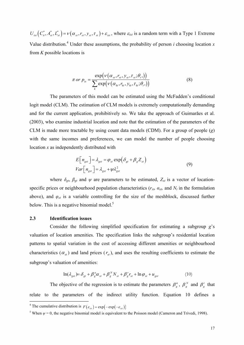
* * *, , , , ,it xt xt xt xt xt xt ixtixtU C A L r y , where ixt is a random term with a Type 1 Extreme

Value distribution.4 Under these assumptions, the probability of person i choosing location x

from K possible locations is

exp , , , ; ,

exp , , , ; ,xt xt xt xt t

ixkt kt kt kt t

k

r yor p

r y

(8)

The parameters of this model can be estimated using the McFadden’s conditional

logit model (CLM). The estimation of CLM models is extremely computationally demanding

and for the current application, prohibitively so. We take the approach of Guimarães et al.

(2003), who examine industrial location and note that the estimation of the parameters of the

CLM is made more tractable by using count data models (CDM). For a group of people (g)

with the same incomes and preferences, we can model the number of people choosing

location x as independently distributed with

2

expxt gt ggxt gxt

gxt g

xt

gxtxt

E n Z

Var n

(9)

where δgt, βgt and ψ are parameters to be estimated, Zxt is a vector of location-

specific prices or neighbourhood population characteristics (rxt, αxt, and Nt in the formulation

above), and φxt is a variable controlling for the size of the meshblock, discussed further

below. This is a negative binomial model.5

2.3 Identification issues

Consider the following simplified specification for estimating a subgroup g’s

valuation of location amenities. The specification links the subgroup’s residential location

patterns to spatial variation in the cost of accessing different amenities or neighbourhood

characteristics ( xt ) and land prices ( xtr ), and uses the resulting coefficients to estimate the

subgroup’s valuation of amenities:

ln( ) lna N rgxt gt g xt g xt g xt xt gxtN r u (10)

The objective of the regression is to estimate the parameters g , N

g and rg that

relate to the parameters of the indirect utility function. Equation 10 defines a 4 The cumulative distribution is exp expixt ixtF 5 When ψ = 0, the negative binomial model is equivalent to the Poisson model (Cameron and Trivedi, 1998).

18

multidimensional plane in which gxt should be decreasing in land prices and decreasing in

amenity access costs (increasing in convenience).

If there were no unobserved quality variables, equation 10 is identified for a

particular group because the relationship between quality and the market price is non-linear

and increasing in quality. For each unit increase in quality, the price increases by a steadily

increasing amount; consequently, the combination a N rg xt g xt g xtN r has an inverted “U”

shape as quality increases.6 The relationship between price and amenities can be estimated as

an adjunct equation to show how different amenities are valued:

( ) ( )a a N N rxt xt xt xtr f f N (11)

This equation is non-linear, as competition between groups who value amenities differently

leads to increasingly high prices for the highest quality locations. Those with the highest

valuations self-select into the areas they value the most.

Three main econometric problems arise when estimating equation 10. The first

problem is that equation 10 is a demand equation, estimating the number of people of group g

who choose to move into region x given prices, whereas the data are determined by the

interaction of supply and demand factors. There are two aspects to the problem. First, the

number of properties available in each meshblock for people to move into will depend on the

size of the meshblock, controlled for in equation 10 by the factor φxt. Secondly, the

equilibrium price of land in each meshblock may be a decreasing function of the number of

available dwellings, or, equivalently, there is scarcity premium if the number of available

houses is small.

If all households were mobile and real estate markets had zero transactions costs,

the supply of dwellings in a region would be the number of dwellings in that region. In this

case, we could set φxt =Txt, the number of households or dwellings in region x. Given the

negative binomial structure of the equation, the coefficient should be one. If a constant

fraction of households moved out of each area each period, we could also use φxt =Txt, as the

number of available places would be proportional to the number of dwellings.

Real estate markets do not have zero transactions costs, however, and not all

people are mobile. Meshblocks differ in the proportion of dwellings that are normally rented,

or which are relatively low-quality “starter houses.” Consequently, the number of households

6 Note that one side of the inverted “U” may be missing for low- or high-income groups.

19

moving into each meshblock in a five year period will vary because of differences in the

fraction of dwellings vacated and freely available. To take account of these differences, we

set (1 )xt xt xtP where Pxt is population in area x and xt is the fraction of the population

living in houses that are newly occupied in the five year period. To avoid obvious

simultaneity difficulties, we use 1xt as an instrument for xt , assuming some meshblocks

persistently have higher turnover than others. Again, because of the negative binomial

structure of the estimation, we expect the coefficient on the term ln ln ln(1 )xt xt xtP

to be equal to one. We constrain the coefficient on ln(Pxt) to equal one but do not constrain

the coefficient on ln(1-ρxt).

The second econometric issue with estimating equation 10 concerns unobserved

variation in quality. It is inconceivable that the observed measures of accessibility that we

include in the regressions encompass all the dimensions of an area’s attractiveness. When

there are aspects of quality that are unobserved, observed prices are likely to be positively

correlated with observed demand, because they reflect the unobserved characteristics of the

locations. Consider the case where there are two amenities, 1 and 2 , the first observed and

the second unobserved. Ignoring xt , the relationships between quality, prices, and number of

people living in a meshblock can be described by the two-equation system:

1 1 2 2ln( ) rgxt gt g xt g xt g xt gxtr u (12a)

1 1 1 2 2 2( ) ( ) rxt xt xt xtr f f (12b)

The equation that is estimated is

1 1 * * 2 2ln( ) rgxt gt g xt g xt gxt gxt g xt gxtr u u u (12c)

Assuming the amenity is desirable (so both 2g and 2 are positive), failure to take

unobserved amenity 2 into account will result in an upward bias in the estimated coefficient

on land rents ˆ rg in equation 12c and a downward bias on the estimated coefficient of the

observed amenity 1ˆg . The former comes because prices are positively correlated with the

unobserved amenity, so when this amenity has a high value both prices and the number of

people wishing to live in the area will be high. The downward bias on 1ˆg occurs as an offset

to the upward bias on ˆ rg ; since the estimated equation suggests high prices do not deter

20

people from moving in to an area enough, it compensates by suggesting it is because they do

not value the amenity sufficiently.

The root cause of these biases in equation 12c is the correlation between the

innovation *gxtu and the land rent. The standard way to counteract the omitted variable bias is

to find an instrument that is correlated with the land rent but uncorrelated with the innovation

term, and use instrumental variables techniques. Unfortunately, it is not clear that there is a

suitable instrument: essentially a variable whose only influence on demand is through price.

As an alternative strategy, therefore, we use a variable that is a proxy for the unobserved

amenities to minimise the effect of the bias. A plausible candidate for this proxy variable is

the spatially-lagged land price – the land price in neighbouring areas,7 or more particularly,

the component of the neighbourhood land price that cannot be explained by observed

amenities, ,ˆx tWv , where W is a spatial weight matrix.

1' 1 1 1

, , , ,

1' 1 1 1, , , ,

( , )

ˆˆ ( , )

x t x t x t x t

x t x t x t x t

Wr f W v

v Wr f W

(13)

,ˆx tv is the component of neighbourhood prices that is not explained by observed

amenities in the neighbouring areas. The estimate ,ˆx tv is used as a proxy for the omitted

amenities in a second stage demand equation: 1 1 2',ˆln( ) r

gxt gt g xt g xt g x t gxtr v u .

Additional spatially lagged terms ( Wag xtWa ) are included to allow for the direct effect of

spatially-lagged characteristics on location choices.

This approach will not eliminate all of the bias in the estimated coefficients ˆ rg and

1ˆg , as it cannot control for the component of the unobserved amenities that does not change

systematically over space. Nonetheless, since we believe the main components of the

unobserved amenities are spatially persistent, the remaining bias should be small.

The third econometric issue with estimating equation 10 arises from the

simultaneity of location choice and area characteristics. This is clearly a problem for

population composition measures. For instance, the proportion of a meshblock’s population

that is foreign born in the 2006 census is likely to be high in meshblocks where the number of

foreign-born entrants between 2001 and 2006 is high. Similarly, high inflows of entrants may 7 In a few cases, neighbourhood land price is missing, either because the meshblock has no neighbouring meshblocks within 2 km, or because land price information is unavailable. In these cases, we use the meshblock’s own land price as a proxy for neighbourhood land price.

21

be a cause of high land prices if the inflows are associated with an increase in demand for a

meshblock. In equation 10, this leads to a correlation between Nxt and the error term, ugxt

resulting in biased and inconsistent parameter estimates.

Our correction for this problem is to estimate the coefficients (in equation 10

using only the variation in local population characteristics and prices that is unrelated to

current inflows (gxt). Specifically, we use an instrumental variables approach to isolate the

variation in prices and endogenous characteristics that can be predicted from time-lagged

measures of those variables. In the non-linear negative binomial model, a control function

approach is a more appropriate way to implement instrumental variables estimation than the

more familiar approach of replacing endogenous variables with their predicted values.8 The

control function approach entails including in the regression additional variables that capture

the endogenous component of the simultaneously-determined variables.

The additional variables are created by running first-stage linear regressions of

each endogenous variable on time-lagged prices, endogenous amenities, and exogenous or

time-invariant measures. The residuals from these first stage regressions are then included in

equation 10. The resulting estimates of the parameters in equation 10 will then be

unbiased.9

In summary, equation 14 is the final form of our estimating equation, estimated

using a negative binomial regression specification with E[ngxt | X] = λgxt.

ln ln ln(1 )gxt gt xt g xt

N rg xt g xt g xt g xt

W WNg xt g xt

N N r rg xt g xt g xt g xt g xt gxt

P

N r

W WN

e e e e e u

(14)

The proxy for unobserved amenities (xt ) is the residual from the following

regression:

1 1 1 1 1ln ln 1P N r

xt t xt xt xt xt xt

W WNxt xt xt

Wr P N r

W WN

(15)

8 For a discussion of the consistency of control function approaches for non-linear models, see Blundell and Powell (2003), Blundell and Smith (1989), Terza (1998), and Wooldridge (2002). 9 Due to the inclusion of these “generated regressors” in our estimating equation, the standard errors that we report will be understated. Correct standard errors can be obtained using bootstrap methods though these are not currently implemented in our estimates.

22

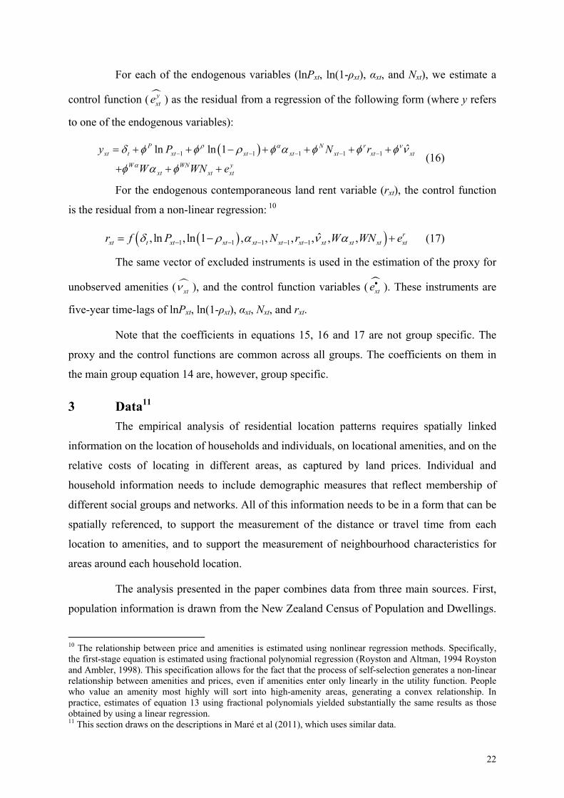
For each of the endogenous variables (lnPxt, ln(1-ρxt), αxt, and Nxt), we estimate a

control function (yxte ) as the residual from a regression of the following form (where y refers

to one of the endogenous variables):

1 1 1 1 1 ˆln ln 1P N r

xt t xt xt xt xt xt xt

W WN yxt xt xt

y P N r

W WN e

(16)

For the endogenous contemporaneous land rent variable (rxt), the control function

is the residual from a non-linear regression: 10

1 1 1 1 1 ˆ, ln , ln 1 , , , , , , rxt t xt xt xt xt xt xt xt xt xtr f P N r W WN e (17)

The same vector of excluded instruments is used in the estimation of the proxy for

unobserved amenities ( xt ), and the control function variables (xte ). These instruments are

five-year time-lags of lnPxt, ln(1-ρxt), αxt, Nxt, and rxt.

Note that the coefficients in equations 15, 16 and 17 are not group specific. The

proxy and the control functions are common across all groups. The coefficients on them in

the main group equation 14 are, however, group specific.

3 Data11

The empirical analysis of residential location patterns requires spatially linked

information on the location of households and individuals, on locational amenities, and on the

relative costs of locating in different areas, as captured by land prices. Individual and

household information needs to include demographic measures that reflect membership of

different social groups and networks. All of this information needs to be in a form that can be

spatially referenced, to support the measurement of the distance or travel time from each

location to amenities, and to support the measurement of neighbourhood characteristics for

areas around each household location.

The analysis presented in the paper combines data from three main sources. First,

population information is drawn from the New Zealand Census of Population and Dwellings.

10 The relationship between price and amenities is estimated using nonlinear regression methods. Specifically, the first-stage equation is estimated using fractional polynomial regression (Royston and Altman, 1994 Royston and Ambler, 1998). This specification allows for the fact that the process of self-selection generates a non-linear relationship between amenities and prices, even if amenities enter only linearly in the utility function. People who value an amenity most highly will sort into high-amenity areas, generating a convex relationship. In practice, estimates of equation 13 using fractional polynomials yielded substantially the same results as those obtained by using a linear regression. 11 This section draws on the descriptions in Maré et al (2011), which uses similar data.

23

Second, land price information is obtained from valuation summaries provided by Quotable

Value New Zealand. Third, information on the location of amenities is assembled from

Geographic Information System (GIS) files obtained from a variety of sources.

3.1 Population location – Census of Population and Dwellings

The New Zealand Census of Population and Dwellings is conducted every five

years and collects a range of socio-demographic information on each member of the New

Zealand population. In the current study, we restrict our attention to people aged 18 years of

age and over, living in the Auckland Urban Area. Our focus on residential location requires

information at a fine spatial scale. The finest geographic breakdown available for Census data

is at the meshblock level. A meshblock is a relatively small geographic area. In urban areas, it

is roughly equivalent to a city block. Within the Auckland Urban Area, there are 8,837

meshblocks, with a median usually resident total population in 2006 of 129 people. In order

to use detailed geographic identifiers, we needed to access the Census data within Statistics

New Zealand’s secure data laboratory and under conditions designed to give effect to the

security and confidentiality provisions of the Statistics Act 1975.12 From this, we obtain

counts of the usually resident population for each meshblock separately for individuals with

particular characteristics, such as sex, age, ethnicity, country of birth, and income band.

We use data from the 1996, 2001 and 2006 Censuses. Self-reported ethnic

identification is collected in the Census, with each person able to select multiple responses.

We report ethnicity on a “total response” basis, which is the approach recommended by

Statistics New Zealand (2005). Individuals giving multiple responses are included in more

than one ethnicity group. Total personal income is reported in 14 categorical bands, which we

summarise at a higher level of aggregation. Where people do not provide a usable response to

the Census questions that we use, they are not included in subgroup counts.

Household income is estimated by aggregating incomes within a dwelling and

adjusting for the number of people. Household income is equivalised by dividing total

household income by the square root of the number of individuals, as in Atkinson et al.

(1995). Where income is missing for some individuals within the dwelling, either because an

individual was absent on census night or because a valid response was not recorded, the

individual is assigned the mean income of other residents at the dwelling.

12 See Statistics New Zealand (2007) for more details on classifications and confidentiality protections.

24

3.2 QVNZ Land Value

The land value measures used in this paper are based on valuation data obtained

from Quotable Value New Zealand (QVNZ), which is New Zealand’s largest valuation and

property information company. For each year, QVNZ assigns the most recent valuation to a

property, and then aggregates all the properties at the meshblock level. Valuations are

available using Statistics New Zealand’s 2001 meshblock boundaries. These have been

mapped to 2006 meshblock boundaries. Land value is measured as the total land value of all

assessments divided by the total land area for all assessments. We restrict attention to

valuations for the Auckland Regional Council area.

Observations are for a category of land use for a meshblock in a valuation year.

Valuations are carried out on a three-yearly cycle, which varies across Territorial Authorities.

Data are available from 1990 for Papakura and Franklin, from 1991 for North Shore,

Auckland, and Manukau, and from 1992 for Rodney and North Shore. Since valuations are

not always available in the census years, they are imputed.

Observations are dropped where the recorded land area is zero or if the number of

assessments is less than three (a combined loss of 6 percent of assessments, 10 percent of

land value). Some observations appear to be outliers in terms of changes in land value per

hectare or land area per assessment. Outliers are identified by regressing each of these

variables on a set of year and indicator variables for each combination of meshblock and

category, and selecting observations with large regression residuals in both regressions.

Affected observations account for around 0.1 percent of assessments and 0.3 percent of

aggregate land value. For these observations, land area per assessment is replaced with the

mean value for the meshblock-category combination and land price per hectare is replaced

with the ratio of total land value to the imputed mean multiplied by the number of

assessments. To reduce remaining volatility, land price per hectare was smoothed using a

three-year moving average across valuation years.

To create an annual land price series from the three-yearly valuation data, we use

annual data on property sales by area unit. (There are approximately 25 meshblocks in each

area unit.) For each valuation year, we calculate the ratio of land price per hectare to median

sales price, and linearly interpolate (and extrapolate for initial and final years, where

necessary) this ratio. Multiplying the observed annual median sales price by this ratio

generates an annual series for land price per hectare. To reduce remaining volatility, land

price per hectare was smoothed using a three-year moving average.

25

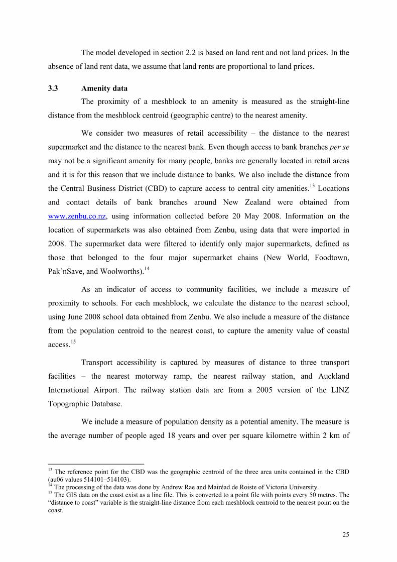
The model developed in section 2.2 is based on land rent and not land prices. In the

absence of land rent data, we assume that land rents are proportional to land prices.

3.3 Amenity data

The proximity of a meshblock to an amenity is measured as the straight-line

distance from the meshblock centroid (geographic centre) to the nearest amenity.

We consider two measures of retail accessibility – the distance to the nearest

supermarket and the distance to the nearest bank. Even though access to bank branches per se

may not be a significant amenity for many people, banks are generally located in retail areas

and it is for this reason that we include distance to banks. We also include the distance from

the Central Business District (CBD) to capture access to central city amenities.13 Locations

and contact details of bank branches around New Zealand were obtained from

www.zenbu.co.nz, using information collected before 20 May 2008. Information on the

location of supermarkets was also obtained from Zenbu, using data that were imported in

2008. The supermarket data were filtered to identify only major supermarkets, defined as

those that belonged to the four major supermarket chains (New World, Foodtown,

Pak’nSave, and Woolworths).14

As an indicator of access to community facilities, we include a measure of

proximity to schools. For each meshblock, we calculate the distance to the nearest school,

using June 2008 school data obtained from Zenbu. We also include a measure of the distance

from the population centroid to the nearest coast, to capture the amenity value of coastal

access.15

Transport accessibility is captured by measures of distance to three transport

facilities – the nearest motorway ramp, the nearest railway station, and Auckland

International Airport. The railway station data are from a 2005 version of the LINZ

Topographic Database.

We include a measure of population density as a potential amenity. The measure is

the average number of people aged 18 years and over per square kilometre within 2 km of

13 The reference point for the CBD was the geographic centroid of the three area units contained in the CBD (au06 values 514101–514103). 14 The processing of the data was done by Andrew Rae and Mairéad de Roiste of Victoria University. 15 The GIS data on the coast exist as a line file. This is converted to a point file with points every 50 metres. The “distance to coast” variable is the straight-line distance from each meshblock centroid to the nearest point on the coast.

26

each meshblock centroid. Our regression specifications include the log of population as a

control, so density is captured by including the log of land area, multiplied by -1.

A measure of proximity to employment is derived from Statistics New Zealand’s

prototype Longitudinal Business Database (LBD). See the disclaimer at the front of this paper

for the conditions of access. Employment accessibility is measured as the ratio of

employment within 2 km of a meshblock to resident population aged 18 and over within 2 km

of a meshblock. Employment in each firm is measured as the annual average number of

employees in each firm at the fifteenth of each month. The meshblock measure of

employment is the sum of employment in plants within the meshblock.16

In order to account for variation in the nature of the housing stock, we include a

measure of the percentage of dwellings in the meshblock that are detached dwellings. This is

one of the few attributes of dwellings that we have consistently across all of the census years.

Finally, we include the percentage of residents living in rental housing. Interpretation of this

variable is difficult, given that the presence of rental properties is correlated not only with

housing quality but also with relatively high turnover.

3.4 Population composition

Previous studies of residential location in Auckland have highlighted the strength

of residential segregation along dimensions such as ethnicity, income, and education (Maré et

al, 2011; Johnston et al, 2010; Pinkerton, 2010). In order to gauge the importance of these

features in residential location decisions, we include in our regressions a range of population

composition measures. We include measures of composition by ethnicity, by country of birth,

by education, and by age. We also include mean equivalised household income to allow for

stratification by income and socioeconomic status.

We include these composition measures for the meshblock as well as for the

meshblocks that are within a 1 km radius. In the few cases where meshblocks are more than 1

km from any other meshblock, we use the composition of the meshblock itself as an indicator

of neighbourhood composition.

4 Results

In a companion paper, we have shown that there is considerable variation in where

different groups locate within the Auckland Urban Area (Maré et al, 2011). In the current

16 Plants are defined by “permanent business numbers” (PBN) as defined in Seyb, 2003.

27

paper, we focus our attention on the location choices of a subset of Auckland residents –

those entering the Auckland Urban Area. Moreover, we restrict attention to people entering

from outside the Auckland Regional Council area, to remove the influence of short-distance

and purely residential moves. People entering Auckland are more likely to be choosing from

among a wide range of possible locations, whereas short-distance moves will often be

constrained by the desire to maintain existing networks and local commitments. The choices

of entrants are therefore likely to provide a clearer picture of the relative importance of

different locational factors.

For all of our analyses, we focus attention on the Auckland Urban Area, which

accounts for around 93 percent of the population and about 7 percent of the land area of the

Auckland Regional Council area. The relatively low population density in meshblocks

outside the urban area, and the larger land area of non-urban meshblocks, make them less

suitable for our analyses.17

4.1 Area characteristics – data description

Table 1 summarises the meshblock data used in our analyses. It shows means and

standard deviations of selected variables for 16,216 meshblock-year observations from the

2001 and 2006 censuses. The first two columns show unweighted means and standard

deviations across meshblocks. The third and fourth columns show these statistics weighted by

population size, to provide a picture of the Auckland Urban Area population.

In 2006, the average meshblock had a usually resident population aged 18 years

and over of 99.6 people. Because larger meshblocks by definition contain more people, the

population weighted average is higher – at 127.8. The average person lives in a meshblock

with 127.8 people.

Means are provided for the land price, density and employment measures as they

are used in subsequent regression analysis. Land price is measured in logs, and has an

average of 14.66 across the two Census years. The average was 0.67 higher in 2006 than it

was in 2001, implying an approximate doubling of land prices (exp(0.67)-1 = 95% increase).

In the average meshblock, 73 percent of dwellings were detached dwellings and the log of

employment was 2.73 (geometric mean employment of 15 jobs). Since subsequent

17 Distance measures are less accurate for large meshblocks and population composition measures are more volatile due to small numbers. Within the Auckland Urban Area, the density of population aged 18 and over is around 800 per square km, compared with 4 per square km outside the urban area (comparable numbers for total population are 1,100 and 6). Around a quarter of meshblocks outside the Urban Area have randomly rounded population counts of 12 or fewer whereas within the Urban Area, the proportion is five percent.

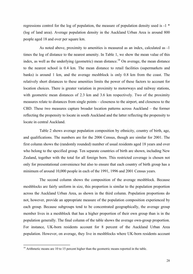
28

regressions control for the log of population, the measure of population density used is -1 *

(log of land area). Average population density in the Auckland Urban Area is around 800

people aged 18 and over per square km.

As noted above, proximity to amenities is measured as an index, calculated as -1

times the log of distance to the nearest amenity. In Table 1, we show the mean value of this

index, as well as the underlying (geometric) mean distance.18 On average, the mean distance

to the nearest school is 0.4 km. The mean distance to retail facilities (supermarkets and

banks) is around 1 km, and the average meshblock is only 0.8 km from the coast. The

relatively short distances to these amenities limits the power of these factors to account for

location choices. There is greater variation in proximity to motorways and railway stations,

with geometric mean distances of 2.3 km and 3.6 km respectively. Two of the proximity

measures relate to distances from single points – closeness to the airport, and closeness to the

CBD. These two measures capture broader location patterns across Auckland – the former

reflecting the propensity to locate in south Auckland and the latter reflecting the propensity to

locate in central Auckland.

Table 2 shows average population composition by ethnicity, country of birth, age,

and qualifications. The numbers are for the 2006 Census, though are similar for 2001. The

first column shows the (randomly rounded) number of usual residents aged 18 years and over

who belong to the specified group. Ten separate countries of birth are shown, including New

Zealand, together with the total for all foreign born. This restricted coverage is chosen not

only for presentational convenience but also to ensure that each country of birth group has a

minimum of around 10,000 people in each of the 1991, 1996 and 2001 Census years.

The second column shows the composition of the average meshblock. Because

meshblocks are fairly uniform in size, this proportion is similar to the population proportion

across the Auckland Urban Area, as shown in the third column. Population proportions do

not, however, provide an appropriate measure of the population composition experienced by

each group. Because subgroups tend to be concentrated geographically, the average group

member lives in a meshblock that has a higher proportion of their own group than is in the

population generally. The final column of the table shows the average own-group proportion.

For instance, UK-born residents account for 8 percent of the Auckland Urban Area

population. However, on average, they live in meshblocks where UK-born residents account

18 Arithmetic means are 10 to 15 percent higher than the geometric means reported in the table.

29

for 12 percent of the population. A comparison of the third and fourth columns of the table

provides an indication of the extent of geographic isolation for each group. An index of

isolation is included in the final column. This expresses the difference between the own-

group proportion and the population proportion as an index between zero and one. A value of

zero arises when a group is located in proportion to the overall population. A value of one

arises when the group lives only in areas with nobody from any other group.19

4.2 Valuation of amenities

The attractiveness of different meshblocks will be reflected in land prices. The

relationship between land price and amenities does not, however, provide an accurate picture

of the trade-offs that any particular person is making. The relationship reflects a combination

of valuations and sorting.

The relative land price premium for different local area attributes reflects the

equilibrium differences in price, and not necessarily the premiums paid by any particular

individual. It is likely that different people have different preferences, and are therefore

willing to pay different premia for locating near amenities that they value. The people who

are observed locating in an area are not a random sample of people. They are the ones who

are willing to pay the highest price to locate there. The premium for location near to the

coast, for instance, is the difference between the value of coastal amenities for those who

value the coast most highly, and the value of non-coastal amenities for those who value the

coast less. The premium thus understates the valuation for those who live near the coast, and

overstates the valuation for those who live away from the coast.

The first stage of our empirical analysis is to examine the overall (equilibrium)

relationship between amenities and land price. This equilibrium relationship is the benchmark

on which entrants to Auckland base their location choices. The parameters presented in Table

3 show the relative land price premium for different local area attributes. The first column

reports regression coefficients on amenities from a series of bivariate regressions of the

following form: ln jt t jt jtP a bZ e , where Zjt is one of the accessibility/amenity measures

that are considered in subsequent analyses. These bivariate patterns confirm the price

premium associated with desirable amenities.

19 The isolation index is the same as that used by Cutler et al. (1999). The formula is I = (ox - px)/(1 - px) where ox is the own-group share and px is the population share.

30

The first two entries in column 1 of Table 3 show that there is considerable

autocorrelation in prices across time (coefficient of 0.86) and spatially (coefficient of 0.94).

Prices are higher in areas with large populations (0.06), in smaller meshblocks (0.57), and in

meshblocks with relatively high proportions of their population new to the area (0.70).

Closeness to amenities also attracts price premia, with a premium for closeness to

supermarkets (0.048 log points, or 4.9 percent higher prices for a 10 percent reduction in

distance), banks (0.064 or 6.6%), the coast (0.010 or 1%), and schools (0.030 or 3%). A 10

percent increase in proximity to the motorway is associated with a three percent premium,

whereas meshblocks near railway stations, which are primarily in West Auckland, are

relatively low priced. South Auckland meshblocks near the Airport are relatively low priced

(-0.025 or -2.5%), whereas a 10 percent increase in closeness to the CBD is associated with a

0.098 log point or 10 percent increase in land price. Meshblocks with more jobs are higher

priced (0.010 or 1 percent higher for a 10 percent increase in the number of jobs), though the

premium is even higher if the wider neighbourhood is job-rich – 0.054 log points or 5.5

percent higher when there are 10 percent more jobs within 2 km of the meshblock.

Meshblocks with higher percentages of people renting are higher priced, as are meshblocks

with a lower proportion of detached housing.

There is clear evidence of population sorting across different priced areas. High

land prices are seen in areas where the population has high household incomes (elasticity of

1.1) or high levels of qualifications (a one percentage point higher fraction of the population

with higher qualifications is associated with 4.8 percent higher prices). Relatedly, country-of-

birth-groups that have relatively low qualification levels (Samoa, Fiji, Tonga) tend to locate

in lower-priced areas. High-priced areas are also associated with relatively high proportions

of 18–30 year olds (a one percentage point higher fraction of 18–30 year olds is associated

with 0.5 percent higher prices) and people aged over 65 years (1.2 percentage points higher).

These bivariate regressions are useful in confirming observed relationships

between prices and amenities. However, it would be wrong to infer that a premium

associated with any particular amenity reflects the desirability of that amenity. The different

measures of attractiveness are correlated, and we wish to control for the influence of other

factors. This is done in column 2 of Table 3, which enters all of the variables in the first

column (other than lagged land price variables) in a single regression. The relationship

between land prices and high population density is relatively unchanged (0.53) and in many

cases the estimated influence of amenities that are correlated with density declines. In

31

particular, the strength of the relationship of land prices to proximity to retail, community,

and transport amenities declines markedly, and in some cases becomes negative. The

correlations between density and each of these measures is in the range of 18 percent to 35

percent. The land price premia seen in column 1 are in part reflecting the fact that these

amenities are more prevalent in dense areas. When density is controlled for, the independent

link with prices is less pronounced.

The estimates in column 1 reveal marked differences in the propensity of different

country-of-birth and ethnic groups to live in high-priced areas. These differences are much

smaller in column 2, indicating that differences in land prices are largely accounted for by

differences in the observed characteristics of the local area, rather than the ethnic or country-

of-birth composition of the area per se. 20 For instance, the strongly positive relationship

between land price and the proportion of Australians in a meshblock becomes small and

statistically insignificant once we control for the influence of correlated factors such as high

household incomes and qualification levels in the area, and distance from the CBD.

The price gradient associated with educational qualifications is reduced to 1.4 (0.69

- (-0.7046)),21 reflecting controls for price-related amenities that are correlated with the

qualification composition. Once we control for other area characteristics, a positive age

gradient becomes evident, with higher land prices in areas with an older age structure.

Not all dimensions of a meshblock’s attractiveness are captured in the variables we

are able to measure. In order to control for omitted area characteristics that may influence

land price, we include, in column 3, the average land price for surrounding meshblocks

within 2 km of each meshblock. This controls for omitted characteristics that are correlated

across space, although not for unobserved characteristics that are idiosyncratic (meshblock-

specific). The coefficient on neighbourhood price is positive and significant (0.66), indicating

a high degree of spatial autocorrelation.22

20 The interpretation of the coefficients on population composition measures differs between column 1 and column 2. In column 2, the effects are relative to groups that are omitted from the regression (percent born in New Zealand, percent with medium qualifications, percent aged 51–64). Since the percentages across all countries of birth, qualification groups, or age groups add to 100 percent, one group must be omitted. For ethnicity, European ethnicity is omitted, although because people can claim multiple ethnicities, the ethnicity percentages add to more than 100 percent. 21 A one percentage point increase in the proportion of high-qualified people, achieved by lowering the proportion of low-qualified people, and holding the share of medium-qualified constant, is associated with 1.4 percent higher land prices. 22 The high (0.94) coefficient on spatially lagged prices in the bivariate regression confirms the high degree of correlation. In the presence of spatial autocorrelation, the parameter estimates are not consistent, and the

32

The coefficients on the amenity and population characteristic variables capture the

degree to which the market valuation of each local feature is higher or lower than would be

predicted from other observed characteristics and the price premium observed in

neighbouring areas. There are, as expected, pronounced reductions in the estimated influence

of measures that are themselves spatially correlated – distance from the airport or CBD, and

neighbourhood employment. There are somewhat reduced age and qualification gradients.

The overseas-born variables have coefficients that are negative, except for

Australian born, and indicate that a 1 percentage point increase in the proportion of a

particular foreign-born group is associated with 0 percent to 1.4 percent lower prices than

could be predicted on the basis of observable characteristics and neighbourhood prices. There

are several possible explanations for these patterns. It may be that foreign-born people are

attracted to meshblocks that are close to amenities that are not highly valued by native-born

New Zealanders. For instance, it could be that the foreign born value different aspects of

schools from native-born New Zealanders. It may be that the presence of foreign-born people

(including the English born) has a depressing effect on prices or it may be that foreign-born

people may simply be more price-sensitive and thus seek under-priced areas.

In column 4, we again include the observed characteristics and contemporaneous

price of neighbourhood meshblocks but in addition control for the price in the previous

period, including the time-lagged price level controls for the impact of unobserved

meshblock-specific amenities that are constant over time. The coefficients on the other

amenities measure how much each amenity can predict prices, conditional on knowing the

lagged prices and prices in neighbouring areas. Column 5 reports the same regression, except

that the observed characteristics are lagged; the coefficients for these two regressions are very

similar.

Not surprisingly, the coefficients on measures that do not vary over time, such as

the proximity to retail, transport and community facilities, are small. In both columns 4 and 5,

the coefficients on schools and supermarkets are small and negative (-0.02 and -0.05), while

the coefficients on banks are small and positive (+0.022 and +0.026). Since it is possible to

improve predictions of contemporary prices by incorporating information about the

unchanging distance to these amenities, these coefficients indicate a small change in the

market valuation of proximity to schools and shopping facilities through time. The coefficient

standard errors will be wrong. An econometric correction would require the calculation of the determinant of a 16,216 by 16,216 matrix, which proved infeasible with available software.

33

on the distance to the Auckland CBD (-0.01) has the same interpretation, suggesting the value

of being near the centre decreased slightly.

Other variables that prove useful in explaining the variation in land prices

conditional on knowing the lagged prices and neighbourhood prices are population density;

the fraction renting; and the fraction of the population born in various overseas countries

including the United Kingdom, China, Korea, and Samoa.

The coefficients in columns 4 and 5 are typically nearer to zero than in column 3.

Since population characteristics are persistent through time, some of the estimated

relationship between prices and population characteristics in captured by the previous price.

The overseas-born variables have coefficients typically from -0.2 to -0.5, indicating that a 1

percentage point increase in the proportion of a particular foreign-born group is associated

with 0.2 percent to 0.5 percent lower prices than could be predicted on the basis of lagged

and neighbourhood price information.

4.3 Patterns of inflows

The price premia shown in Table 3 associated with features such as density, renting

proportion, mean income, and employment accessibility indicate that, in equilibrium, people

are willing to pay a premium to be located in meshblocks with high values of these amenities.

We now turn to the primary focus of our study: whether population location decisions reflect

the presence of such amenities. In this section, we examine the location choices of various

subgroups of entrants into Auckland – defined by country of birth, ethnicity, household

income, or qualifications. Table 4 summarises the size of the various groups of entrants, and

some of their key characteristics.

According to the 2006 Census, there were 884,50023 people aged 18 and over who

were usually resident in the Auckland Urban Area. Of these, 28 percent (246,600) were living

outside the Auckland Region five years earlier. We refer to these people as “entrants”. These

entrants account for around half of all people in the Auckland urban area who had changed

addresses in the previous five years.

Compared with the usually resident population (aged 18 and over), people entering

the Auckland Urban Area from outside the Auckland Region are, on average, more highly

qualified, younger, less likely to be employed full-time, and more likely to be renting, and 23 All counts from the census have been randomly rounded to base 3, in accordance with Statistics New Zealand’s Census Confidentiality Rules (Statistics New Zealand, 2007), and then rounded to the nearest 100 for presentational purposes.

34

they have slightly lower household incomes. They are also more likely to be single without

dependants. These characteristics are typical of more mobile populations.

There is, of course, considerable heterogeneity within the population of entrants.

The remainder of Table 4 summarises key characteristics of a range of entrant subgroups.

Differences in entrant characteristics by ethnicity, qualification, income, and country of birth

largely reflect overall population differences by these groupings.

Compared with other ethnicities, entrants of Maori or Pacific ethnicity have lower

qualifications, a relatively young age structure, relatively low household income, and have a

high probability of living in a rented dwelling. A relatively large share of Maori entrants are

in households with a single adult, either with dependants (45%) or without dependants (14%).

Entrants of Pacific ethnicity are more likely to be in “couple with dependant” households,

and have somewhat lower median household incomes ($31,400) than Maori entrants

($38,800). Entrants of Asian ethnicity have high qualification levels and a relatively young

age structure. They are more likely than other entrants to be in couple households. They have

relatively low full-time employment probabilities (41%), and low median household incomes

($27,400).

Entrant characteristics also vary by qualifications and household income, with

similar patterns for high-income and high-qualification groups, and for low-income and low-

qualification groups. There is a positive correlation between income and qualifications, and

both are positively related to full-time employment probabilities. Entrants with no

qualifications tend to be older (38 percent are over 50, compared with only 20 percent for all

entrants), whereas those with low household incomes are disproportionately younger. The

proportion of entrants in rental dwellings is relatively high for the younger and low household

income groups than it is for those with high household incomes, as both age and income are

positively related to home ownership (Morrison, 2008). There is no difference in renting

probabilities between high- and low-qualification groups – presumably due to the offsetting

effects of income and age differences. The low-qualification entrants have lower incomes but

are generally older.

The final panel of Table 4 shows differences between subgroups of entrants

defined by country of birth. We restrict attention to entrants who were living overseas five

years prior to the census. The countries of birth are ordered from highest to lowest median

household income. Entrants from Australia, the UK and South Africa, and returning New

35

Zealanders have the highest incomes, reflecting in part their older age structure and higher

qualifications. Incomes for Indian entrants are significantly lower, despite having the highest

proportion of graduates and a relatively high share of 31–50 year olds. Among this set of

highly qualified entrant groups, New Zealanders and those from the UK are the least likely to

be renting.

Of the remaining country-of-birth entrant groups, those from Samoa and Tonga

have the lowest qualifications structure, are relatively young, and are very likely to be in

rented accommodation. Fijian entrants are also relatively young, though they have a low

likelihood of being in rental dwellings. Finally, entrants from the People’s Republic of China

and from South Korea have the lowest median household incomes, despite having moderately

high qualifications. A high proportion of Chinese entrants (57%) are in the 18–30 year age

group, reflecting relatively high numbers of international students. The Korean age structure

is more similar to that of returning New Zealanders, with a fairly high proportion of 31–50

year olds (61%). These two groups also have low probabilities of being in rented dwellings,

suggesting that current household income may be a weak proxy for household wealth. Korean

entrants are most likely to be in households with a single adult with dependants (13%),

perhaps reflecting the prevalance of “astronaut families” (immigrant families in which an

adult is absent overseas for prolonged periods: Ho, 2004) or home-based accommodation for

Korean students (Meares et al, 2010).

The final insight from Table 4 is that each of the entrant groups accounts for a

relatively small proportion of the total population. The largest country of birth group (PRC)

accounts for less than 3 percent of the usually resident population. Only the European

ethnicity entrants group accounts for more than 10 percent of the population.

The degree to which these separately identified entrant groups affect relative land

prices will depend on the distinctiveness of their residential location choices and

consequently how concentrated they are in particular meshblocks. The following section

examines patterns of location choice for the various entrant groups.

4.4 Location choice regressions

4.4.1 Treating amenities as unobserved

Table 5 presents regression estimates of equation 14, but with amenities omitted.

These results thus show the systematic relationship between location choice and land rents.

The coefficient on the log of population is constrained to equal one, to serve as an exposure

36

factor in the negative binomial regression (φ in equation 9). This captures the expectation that

the number of entrants into a meshblock should increase in proportion to the population size

of the meshblock. The percent of the population that is new to the area is also included to

allow for variation across meshblocks in the number of available places.

The top panel of Table 5 shows estimates that do not control for the potential

simultaneity of population size and the number of entrants. In the first column, we show

estimates for all inflows from outside Auckland region into the Auckland Urban Area. There

is a negative coefficient of -0.015 on the log of land price, indicating that a 10 percent higher

land price is associated with a 0.15 percent decrease in the likelihood of choosing a

meshblock.24

The relationship between land price and location choice would be positive were we

not including a proxy measure for unobserved amenities. The coefficient on unobserved

amenities is 0.080, indicating that entrants are drawn to places where land prices in

surrounding areas are high. We interpret this attraction as being due to unobserved amenities

that are spatially correlated.

The row labelled ψ is the estimates of the dispersion parameter in equation 9. The

estimate of 0.075 indicates that the variance of the mean number of people entering a

meshblock is 7.5 percent higher than the mean. The fact that this number is significantly

different from zero justifies the use of a negative binomial rather than a Poisson regression

specification. The point estimate and standard error are shown for the log of ψ, which is the

form in which the dispersion parameter is estimated.

The lower panel of Table 5 presents estimates that control for the simultaneity of

the land price, population, and “percent new” variables. As discussed above, this is done by

including residuals from regression of each of these simultaneously determined variables on

their lags and other exogenous variables. The time-lagged average land price is included as

an additional instrument. Controlling for simultaneity leads to a small drop in the coefficient

on land price, consistent with entrants exerting slight upward pressure on land price. Note

that the land price coefficient may still be positively biased as a result of unobserved

amenities. Our inclusion of a proxy based on an unexplained neighbourhood price premium

adjusts for spatially correlated unobserved amenities. It cannot, however, control for the

24 With around 8,000 meshblocks, the base probability of choosing a meshblock is roughly 1 in 8,000. A 10 percent higher probability of selection changes this to around 1 in 7,300. A 0.15 percent decrease scarcely changes the probability (1 in 7,988).

37

possibility that the meshblocks to which entrants are attracted are high priced as a result of

(unobserved) meshblock-specific amenities.

The other columns of Table 5 show estimates for various subsets of entrants.

Columns 2 and 3 display estimates for entrants who were living outside New Zealand five

years before the census date. These are divided into foreign-born (“recent migrants”) and

New Zealand-born (“returning New Zealanders”). The remaining columns show results by

equivalised household income and level of qualifications. For each of these dimensions, we

focus on entrants with income or qualification levels that are approximately in the top third

and in the bottom third of the overall population. A person’s level of qualifications is a better

proxy for lifetime income than is current household income. We would expect to see more

systematic patterns of location choice by qualification than by current income level.

Qualifications are also more exogenous, in the sense that they are unlikely to be a

consequence of where entrants choose to live, whereas the level of household income may

depend on location.

Our discussion of Table 5 focuses on the lower panel, which controls for the

potential simultaneity of land prices and the number of entrants. The estimates for recent

migrants are similar to those for all entrants, showing a pattern of attraction to unobserved

amenities (coefficient of 0.149) and a weak deterrent effect of low prices (a statistically

insignificant coefficient of -0.014). For returning New Zealanders, the attraction from

unobserved amenities is stronger, with a coefficient of 0.335. This indicates that returning

New Zealanders are relatively strongly attracted to meshblocks with unobserved amenities

that are capitalised into neighbourhood land prices. As shown in Table 4, returning New

Zealanders have relatively high household incomes and qualifications. We hypothesise that

whatever the unobserved amenities are, they are amenities that are most attractive to high-

income and highly qualified entrants, as the preferences of such groups are most readily

capitalised into land prices. This interpretation is corroborated by the fact that the estimated

attractiveness of unobserved amenities is also strong for entrants with high household

incomes (0.226) and high qualifications (0.443), but is weak for those with low household

incomes (0.069) and negative for those with low qualifications (-0.154).

The estimated effect of land prices on location choices is positive for high-income

and high-qualification groups, suggesting that these entrants are attracted by high prices. We

would have expected high prices to be a deterrent. A positive relationship may arise if the

price of a location is used as a signal of status (i.e.: if prime location is a “Veblen good”), or

38

if people buying their residence in high-priced areas expect greater capital gains. Instead, our

interpretation is that our control for unobserved amenities is incomplete, and that there is a

positive correlation between prices and location choices because of unobserved factors that

are capitalised into land prices. This capitalisation is strongest for high-income and high-

qualified entrants. In contrast, low-qualified entrants and, to a lesser extent, low-income

entrants are, as expected, deterred by high land prices – with coefficients of -0.239 and -0.099

respectively.

Table 6 presents comparable estimates for four groups of entrants defined in terms

of ethnicity. The four groups are arranged in ascending order of median household income.

The highest-income ethnic group, European entrants, accounts for around 40 percent of all

entrants, and shows patterns of location choice similar to the high-household income group in

Table 5. European entrants are attracted to areas with high unobserved amenities, and the

coefficient on land price is positive. Entrants of Maori and Pacific ethnicity have similar

patterns, consistent with the patterns previously seen for low-income and low-qualification

entrants. Asian entrants are attracted by unobserved amenities in the same way as European

entrants but appear to be less sensitive to land price. The mixed results for the group of Asian

ethnicity entrants may also reflect the considerable diversity within the category, including as

it does entrants from many different countries and cultures, and including new entrants as

well as established migrants and New Zealand-born Asians.

In order to investigate further the diversity of patterns within broad ethnic groups,

Table 7 presents estimates for recent migrants – those who arrived in New Zealand in the

previous five years – disaggregated by country of birth. We exclude foreign-born entrants to

Auckland who were already living in New Zealand five years previously. Analysis by

country of birth reveals variation between subgroups, especially within the broad Asian and

Pacific ethnic groups. As in Table 6, the groups are presented in ascending order of

household income. Recent migrants from South Korea and the People’s Republic of China

have relatively low household incomes, but relatively high qualifications. Price effects are

positive for Korean entrants but they do not appear to respond to our proxy for unobserved

amenities. It may be that the amenities to which they are attracted are inadequately captured

by our spatially correlated proxy. In contrast, the location choices of Chinese entrants reflect

an attraction to unobserved amenities and a moderately strong deterrent effect of high land

prices.

39

For other country-of-birth groups, the impact of price variation (controlling for

unobserved amenities) follows an income gradient, with lower income groups more strongly

deterred by high prices. The impact of unobserved amenities is less systematic, pointing to

the potential gains of including observed amenity measures in the regression. For instance,

while Fijians and Samoans have difficult-to-understand significant negative coefficients on

the unobserved amenity variable in Table 7, when observed amenities are included in the

regression in Table 10, the coefficients become much closer to zero and statistically

insignificant.

4.4.2 Including observed amenity measures

In this section, we discuss regression estimates of equation 14, including

meshblock-level measures of amenities. Including these measures reduces the importance of

our proxy for unobserved amenities. The unobserved amenity proxy now identifies only

unobserved amenities that are uncorrelated with the included measures, and correlated

spatially. All of our measured amenities vary across meshblocks, and all except the proximity

measures vary over time as well. The augmented regressions presented in this section attempt

to identify more meaningfully the characteristics of meshblocks that different groups of

entrants find attractive.

Table 8 provides estimates for the broadly defined entrant groups considered in

Table 5. For all entrants, shown in the first column, the price elasticity is similar to that in

Table 5. The impact of unobserved amenities is, as expected, greatly reduced due to the

inclusion of measured amenities. It is difficult, however, to identify particular observed

amenities that are strongly and consistently attractive to entrants. This is in part due to

relatively strong correlations between some of the measures. In particular, the density of

employment is strongly correlated with several key amenities such as proximity to

supermarkets ( = 0.34), banks ( = 0.35), schools ( = 0.33), and the CBD ( = 0.34).

Furthermore, each of these variables is correlated with neighbourhood employment – the log

of employment within 2 km of the meshblock and land prices ( between 0.32 and 0.62).

Clearly, dense areas allow greater access to services and employment. They also have higher

land rents. The ability of the regression analysis to identify a primary source of attractiveness

is limited by the strong relationship between the factors.

Overall, the results for all entrants indicate a propensity to locate near the CBD

(0.63 percent increase in probability of selection with a 10 percent decrease in distance from

40

CBD) and away from the airport in the South (0.52 percent decrease in probability with a 10

percent increase in distance from airport). They also favour areas with a low proportion of

detached dwellings (2.1 percent lower probability with a one percentage point increase in the

proportion of dwellings that are detached), and in meshblocks with relatively high

employment (0.2 percent increase in probability of selection with a 10 percent decrease in

employment).

Recent migrant entrants appear to favour meshblocks with high proportions of all

of the country of birth groups that are included as explanatory variables. The New Zealand-

born proportion is excluded, so the coefficients reflect the attractiveness of country of birth

mix relative to the proportion of residents who are New Zealand born. The uniformly positive

coefficients indicate that entrants are drawn to meshblocks where the migrant presence is

high. As will be shown in Table 10, different country of birth groups are drawn to areas

where their compatriates live. The coefficients on country-of birth shares are mostly negative

for the returning New Zealander entrants (with the exception of a positive influence of a high

Australian share), indicating that this group of entrants is attracted to areas where the

proportion of New Zealand born is high. Entrants also tend to locate in areas with a relatively

young population.

There are relatively few statistically significant coefficients for the subgroups of

entrants shown in the remaining columns of Table 8. There is a clear distinction between low-

and high-income entrants, and between high- and low-qualification entrants. Each group is

attracted to meshblocks where their own group tends to locate.25 The coefficient on mean

household income in the meshblock is strongly positive for high-income entrants (0.963).

This implies that the probability of a high-income entrant entering an area increases by 9.6

percent if the median income of the area is 10 percent higher. The effect of median income is

strongly negative for low-income entrants (-1.173). Similarly, meshblocks with a high

proportion of high-qualified residents attract high-qualified entrants (2.314) and deter low-

qualified entrants (-1.688).26

The attraction of like individuals is the strongest regularity in the patterns of

location choice for entrants defined by country-of-birth or ethnicity entrant groups. Table 9

25 The instrumental variables approach of using control functions has the greatest impact on coefficients for “own-group” attraction. This is true across income, qualification, ethnicity, and country of birth. Specifically, the use of IV methods greatly reduces the size of coefficients, as a result of controlling for the direct contribution of the entrants to the composition measures. 26 The coefficients on the meshblock qualification proportions reflect the attractiveness relative to the proportion of the omitted (medium qualification) group.

41

shows the results for entrants defined by ethnicity. Maori entrants are attracted to areas with a

high proportion of Maori residents. A one percentage point increase in the proportion of

Maori residents raises the probability of Maori entrants choosing the area by 2.8 percent.

Asian entrants are attracted to areas with a high proportion of Asian residents (2.3%) and

Pacific entrants are attracted to areas with high Pacific populations (1.8%) and also those

with high Maori populations (1.6%). Asian-ethnicity entrants are attracted by proximity to

schools (0.029) and supermarkets (0.080), and to areas with more employment in the

surrounding 2 km (0.059). The inclusion of the additional covariates also yields a substantial

increase in the measured goodness of fit. The pseudo R-squared statistic increases markedly –

from around 0.02–0.04 in Table 6, to around 0.20 in Table 9 when amenities are included.

Table 10 shows results for entrants defined by country of birth, with the analysis

restricted to entrants who were living out of New Zealand five years earlier. There are some

significant effects of measured amenities but there are few consistent patterns. For all country

of birth groups, the coefficient on land price is positive, indicating that entrants are attracted

to high-priced places or repelled from low-priced places. This result is counter-intuitive and

is perhaps reflecting the greater importance of idiosyncratic unobserved meshblock attributes

in the location choices of more narrowly-defined entrant groups. The coefficient on

population density is negative for all country of birth groups, and statistically significant for

four groups of entrants, those from Korea, China, Fiji, and South Africa. Proximity to

supermarkets is an attractor for Korean, Chinese, Fijian and South African entrants and

neighbourhood employment also attracts entrants from China and India. Koreans and Fijians

tend to locate away from meshblocks with high proportions of renters. Surprisingly, Tongans

and Samoans, who are over-represented in South Auckland, appear to be attracted to the

central city, as are those from China, India, and South Africa.

The strongest pattern revealed in Table 10 is that recent entrant groups defined by

country of birth groups are clearly attracted to meshblocks where their compatriots live. The

coefficients on own-group concentrations are highlighted in boxes in Table 10. The

magnitudes of the coefficients show the relative change in the probability of selecting a

meshblock where all residents are from their country of birth, compared with the probability

of selecting a meshblock with only New Zealand-born residents. In order to provide a more

meaningful indication of the magnitude of own-country effects, we compare the

attractiveness of meshblocks with an average share of compatriots with the attractiveness of

the sort of meshblocks where compatriots tend to locate. As shown in Table 2, due to the

42

geographic concentration of each country of birth group, the average group member lives in a

meshblock where the share of the population that is from their country of birth is higher than

it is in the Auckland Urban Area generally. Table 11 brings together the own-country-of-birth

coefficients from Table 10 and the mean proportions from Table 2. The column labelled

“Increase in probability” shows how much more attractive each country of birth group finds

the meshblocks where their compatriots live than meshblocks with an average share of their

compatriots. Residents born in South Korea, for example, account for two percent of the

Auckland Urban Area population, yet the average South Korean lives in a meshblock where

nine percent of the population is from South Korea. Applying the regression coefficient of

16.75 to this difference, we calculate that a South Korean entrant is 221 percent more likely

(i.e.: 3.2 times as likely) to select a meshblock with nine percent concentration than one with

two percent.27 For groups other than those from South Africa, the UK and Australia, the

effect is to at least double the probability of selection (120% to 262% increases). High own-

group shares in surrounding meshblocks (those within a 2km radius) also increase the

attractiveness of meshblocks. The final column of the table shows the coefficients on

neighbourhood own-group-share. South African, UK and Australian entrants are attracted to

meshblocks in areas where their compatriots are prevalent – even though the attraction of

high-incidence meshblocks is small.

Comparable calculations are shown for ethnicity and qualification groups. For

these groups, own-group attraction raises the probability of selection by 18 percent to 55

percent.

5 Discussion

What determines residential location choices? Location choices reflect a

fundamental trade-off between the desirability of a particular location and the cost of locating

there. In directly modelling the location decisions of people entering the Auckland urban area

from outside the Auckland region, we use econometric methods to separate the deterrent

effect of high land prices from the attractiveness of local amenities. The approach taken in

this paper is innovative. To our knowledge, this is the first paper that estimates the

determinants of intra-metropolitan location choices by all new entrants at a finely partitioned

spatial scale, incorporating land prices, and controlling for unobserved amenities and price

endogeneity. The approach provides a balance between the need for a tractable empirical

27 Calculation: 221%= (exp(*(9%-2%))-1)

43

model, and the need to reflect the complex realities of location choice in large, rapidly

growing modern cities (Anas et al, 1998). By separately examining location choice patterns

for population subgroups with possibly different preferences, we are able to take account of

spatial interactions between groups within local land markets.

We have identified the importance of a range of population characteristics and

local amenities that are important influences on these choices. The estimation results suggest

the population characteristics of an area are particularly important. However, as areas with

attractive amenities are also areas that are highly priced, it is difficult to identify the deterrent

effect of high prices. Yet, without including prices, we can identify where people live but not

why they live there.

As would be expected when amenities are capitalised into prices, we have been

able to identify the importance of a range of local amenities that are separately related to local

land prices. It is difficult to disentangle the independent influence of particular factors

because desirable areas may be desirable on several dimensions. The difficulty is exacerbated

because we do not observe all relevant amenities that determine desirability and land values.

Table 3 shows that many of the positive correlations between amenities and prices are no

longer evident if we simultaneously control for the presence of multiple amenities. As the

land price in a meshblock is strongly related to the lagged land price (lagged either spatially

or temporally), our ability to identify separately the price effects of slowly changing or

spatially correlated amenities is further limited.

In Table 5 to Table 7, we examine the effect of prices, treating all amenities as

unobserved, but including the land price premium in surrounding areas as a proxy for these

unobserved amenities. Overall, we find that entrants are attracted to areas with high

unobserved amenities, with the attraction greatest for high-income and high-qualified

entrants. When we add measures of observed meshblock and wider neighbourhood amenities

in Table 8 to Table 10, the role of unmeasured amenities is greatly reduced, as expected, and

we are able to identify features of meshblocks that are most attractive to entrants.

Overall, high land prices are a deterrent to entrants, yet for subgroups with high

incomes or qualifications, we estimate a positive relationship between land prices and entry.

Our preferred interpretation of this positive relationship is that it reflects the influence of

unobserved amenities that are inadequately captured by our proxy variable. In particular, we

infer that there are meshblock-specific sources of attractiveness that are captured neither by

44

the meshblock-level amenities that we measure nor by spatially lagged price premia. Other

explanations for the positive coefficients on price include the possibility that high-income

groups are attracted to high-priced locations because they serve as a signal of high status, or

because they are believed to offer greater potential for capital gains. Positive coefficients may

also stem from inadequate control for demand fluctuations, which simultaneously generate

both price increases and higher inflows.

The joint impact of controlling for both land prices and unobserved amenities is

that we can interpret the coefficients on the included amenity measures as indicating their

independent influence on location choice, even though we have not been fully successful in

separating the deterrent effect of price from the influence of omitted amenities.

5.1 Main findings

The main result from the amenity-augmented location choice regressions

summarised in Table 8 to Table 10 is the significant role played by “own-group” attraction.

Groups of entrants classified by qualification, income, ethnicity, or country of birth are all

attracted to meshblocks or neighbourhoods where their group already has a strong presence.

In a previous paper (Maré et al, 2011), we documented a high degree of residential sorting by

ethnicity, income, and qualifications. The current paper confirms the importance of such

sorting, and demonstrates that the sorting reflects attraction to fellow group members, rather

than being due to group members having common preferences for local amenities.

The importance of own-group attraction implies that the future spatial patterns of

population growth in Auckland will depend very much on who enters Auckland, or which

groups increase their share of the population. The geography of residential pressures arising

from increases in population will reflect the composition of population increase. Population

subgroups that are becoming more prevalent will put pressure disproportionately on areas

where their group is already located. However, because the location of subgroups appears to

be more strongly connected to own-group selection than to proximity to any physical or fixed

locational amenities, longer-run residential pressure is less predictable. If a subgroup

increases in size, a new concentration may arise away from current concentrations. Examples

of such developments between 1996 and 2006 include entrants from China, who established a

new concentration in the North Shore, and those from India, with a concentration in South

Auckland (Pinkerton et al, 2010). A similar dynamic in the past accompanied the expansion

45

of the Pacific population in the 1970s, which led to a stronger concentration in South

Auckland, and reduction of Pacific population near central Auckland.

The second implication of our findings relates to the relatively weak systematic

evidence on the role of specific location amenities. We are surprised by the apparent lack of

importance of amenities such as access to transport, coastal location, or distance to school

and retail facilities, given the commonly accepted importance of these. We have used a very

fine spatial scale for our analysis, which improves our chances of detecting the attractiveness

of local amenities. However, the coarseness of our amenity measures may have limited our

ability to identify relevant quality dimensions such as school quality, coastal views, and

congestion of transport networks. It may also be that attractive areas are ones that offer a

portfolio of amenities, making it difficult to attribute attractiveness to any one amenity. These

results emphasise that the quality or combination of local facilities is much more important

than the simple availability of facilities. These factors are being picked up by our proxy for

unobserved amenities but are not reflected in the coefficients on our measured amenities.

The results suggest that changes in any specific amenity in isolation will not

necessarily lead to a significant change in either land prices or the probability of people

locating in the area. Residents are attracted to areas that offer a package of amenities that best

suits their needs and budget, given the land price premia that result from other residents’

valuations of the package. Policies that change land prices will have as much effect as

policies that change accessibility to valued facilities. Consequently, the provision of

infrastructure, coordination and planning to support Auckland’s future residential

development needs to be based on an integrated view of the various dimensions of local area

attractiveness and a recognition of not just the innate desirability of different facilities but the

willingness and ability of different groups to pay for them.

46

References Albouy, David. 2009. "What Are Cities Worth? Land Rents, Local Productivity and the

Capitalization of Amenity Values," NBER Working Paper 14981, National Bureau of Economic Research, Cambridge MA.

Alonso, William. 1964. Location and Land Use, Cambridge: Harvard University Press. Anas, Alex; Richard Arnott and Kenneth A. Small. 1998. "Urban Spatial Structure," Journal

of Economic Literature, 36:3, pp. 1426–64. Atkinson, Anthony B.; L. Rainwater and T. Smeeding. 1995. Income Distribution in OECD

Countries: Evidence From the Luxembourg Income Study (LIS), Paris: OECD. Baum-Snow, Nathaniel. 2007. "Did Highways Cause Suburbanization?," Quarterly Journal

of Economics, 122:2, pp. 775–805. Bayer, Patrick and Christopher Timmins. 2005. "On the Equilibrium Properties of Location

Sorting Models," Journal of Urban Economics, 57:3, pp. 462–77. Black, Sandra E. 1999. "Do Better Schools Matter? Parental Valuation of Elementary

Education," Quarterly Journal of Economics, 114:2, pp. 577–99. Blundell, Richard and J. L. Powell. 2003. "Endogeneity in Nonparametric and

Semiparametric Regression Models" in Advances in Economics and Econonometrics: Theory and Applications, Eighth World Congress, Vol. II, Mathias Dewatripont, Lars P. Hansen and Stephen J. Turnovsky, Eds. Cambridge: Cambridge University Press, pp. 312–57.

Blundell, Richard W. and R. J. Smith. 1989. "Estimation in a Class of Simultaneous Equation

Limited Dependent Variable Models," Review of Economic Studies, 56, pp. 37–58. Cameron, A. C. and P. K. Trivedi. 1998. Regression Analysis of Count Data, Cambridge:

Cambridge University Press. Carlton, Dennis W. 1983. "The Location and Employment Choices of New Firms: An

Econometric Model With Discrete and Continuous Endogenous Variables," The Review of Economics and Statistics, 65:3, pp. 440–9. Available online at http://www.jstor.org/stable/1924189.

Cutler, David M. and Edward L. Glaeser. 1997. "Are Ghettos Good or Bad?" Quarterly

Journal of Economics, 112:2, pp. 827–72. Cutler, David M.; Edward L. Glaeser and Jacob L. Vigdor. 1999. "The Rise and Decline of

the American Ghetto," The Journal of Political Economy, 107:3, pp. 455–506. Duranton, Gilles and Matthew Turner. 2008. "Urban Growth and Transportation," CEPR

Discussion Paper 6633, Center for Economic Policy Research, London.

47

Florida, Richard. 2000. "Competing in the Age of Talent: Quality of Place and the New Economy," A Report Prepared for the R.K Mellon Foundation, Heinz Foundation and Sustainable Pittsburgh.

Frost, Lionel. 1991. The New Urban Frontier: Urbanisation and City-Building in Australasia

and the American West, Kensington, NSW: New South Wales University Press. Glaeser, Edward L. and Joshua D. Gottlieb. 2009. "The Wealth of Cities: Agglomeration

Economies and Spatial Equilibrium in the United States," Journal of Economic Literature, 47:4, pp. 983–1028.

Glaeser, Edward L. and Janet Kohlhase. 2004. "Cities, Regions and the Decline of Transport

Costs," Papers in Regional Science, 83:1, pp. 197–228. Gottlieb, Paul. 1994. "Amenities as an Economic Development Tool: Is There Enough

Evidence?" Economic Development Quarterly, 8:3, pp. 270–85. Guimarães, Paulo; Octávio Figueirdo and Douglas Woodward. 2003. "A Tractable Approach

to the Firm Location Decision Problem," The Review of Economics and Statistics, 85:1, pp. 201–4. Available online at http://www.jstor.org/stable/3211633.

Ho, E. 2004. "Mental Health of Asian Immigrants in New Zealand: A Review of Key Issues,"

Asian and Pacific Migration Journal, 13:1, pp. 39–60. Johnston, Ron J.; Michael Poulsen and James Forrest. 2010. "Evaluating Changing

Residential Segregation in Auckland, New Zealand, Using Spatial Statistics," Tijdschrift voor economische en sociale geografie: Journal of Economic and Social Geography. Available online at http://dx.doi.org/10.1111/j.1467-9663.2009.00577.x.

LeRoy, Stephen F. and Jon Sonstelie. 1983. "Paradise Lost and Regained: Transportation

Innovation, Income, and Residential Location," Journal of Urban Economics, 13, pp. 67–89.

Maré, David Christopher; Andrew Michael Guy Coleman and Ruth Pinkerton. 2011.

"Patterns of Population Location in Auckland," Motu Working Paper 11-06, Motu Economic and Public Policy Research, Wellington.

Massey, Douglas S. 2008. "Origins of Economic Disparities: The Historical Role of Housing

Segregation" in Segregation: the Rising Costs for America, James H. Carr and Nandinee Kutty, Eds. New York: Routledge, pp. 39–80. Available online at http:\\books.google.com.

McFadden, Daniel. 1978. "Modeling the Choice of Residential Location" in Spatial

Interaction Theory and Planning Models, Anders Karlqvist, L. Lundquist, F. Snickers and J. Weibull, Eds. Amsterdam: North-Holland, pp. 75–96.

Meares, Carina; Elsie Ho; Robin Peace and Paul Spoonley. 2010. "Kimchi Networks: Korean

Employers and Employees in Auckland," Integration of Immigrants Programme Research Report No. 1/2010, Massey University/University of Waikato, Albany.

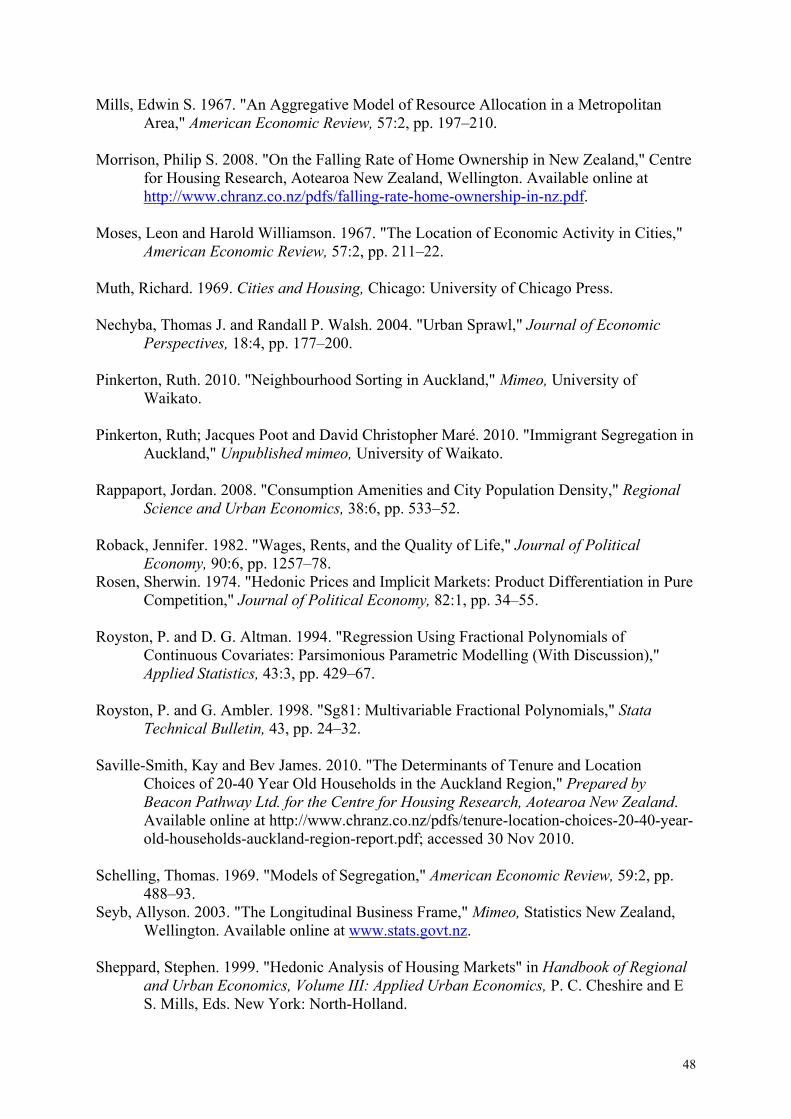
48

Mills, Edwin S. 1967. "An Aggregative Model of Resource Allocation in a Metropolitan Area," American Economic Review, 57:2, pp. 197–210.

Morrison, Philip S. 2008. "On the Falling Rate of Home Ownership in New Zealand," Centre

for Housing Research, Aotearoa New Zealand, Wellington. Available online at http://www.chranz.co.nz/pdfs/falling-rate-home-ownership-in-nz.pdf.

Moses, Leon and Harold Williamson. 1967. "The Location of Economic Activity in Cities,"

American Economic Review, 57:2, pp. 211–22. Muth, Richard. 1969. Cities and Housing, Chicago: University of Chicago Press. Nechyba, Thomas J. and Randall P. Walsh. 2004. "Urban Sprawl," Journal of Economic

Perspectives, 18:4, pp. 177–200. Pinkerton, Ruth. 2010. "Neighbourhood Sorting in Auckland," Mimeo, University of

Waikato. Pinkerton, Ruth; Jacques Poot and David Christopher Maré. 2010. "Immigrant Segregation in

Auckland," Unpublished mimeo, University of Waikato. Rappaport, Jordan. 2008. "Consumption Amenities and City Population Density," Regional

Science and Urban Economics, 38:6, pp. 533–52. Roback, Jennifer. 1982. "Wages, Rents, and the Quality of Life," Journal of Political

Economy, 90:6, pp. 1257–78. Rosen, Sherwin. 1974. "Hedonic Prices and Implicit Markets: Product Differentiation in Pure

Competition," Journal of Political Economy, 82:1, pp. 34–55. Royston, P. and D. G. Altman. 1994. "Regression Using Fractional Polynomials of

Continuous Covariates: Parsimonious Parametric Modelling (With Discussion)," Applied Statistics, 43:3, pp. 429–67.

Royston, P. and G. Ambler. 1998. "Sg81: Multivariable Fractional Polynomials," Stata

Technical Bulletin, 43, pp. 24–32. Saville-Smith, Kay and Bev James. 2010. "The Determinants of Tenure and Location

Choices of 20-40 Year Old Households in the Auckland Region," Prepared by Beacon Pathway Ltd. for the Centre for Housing Research, Aotearoa New Zealand. Available online at http://www.chranz.co.nz/pdfs/tenure-location-choices-20-40-year-old-households-auckland-region-report.pdf; accessed 30 Nov 2010.

Schelling, Thomas. 1969. "Models of Segregation," American Economic Review, 59:2, pp.

488–93. Seyb, Allyson. 2003. "The Longitudinal Business Frame," Mimeo, Statistics New Zealand,

Wellington. Available online at www.stats.govt.nz. Sheppard, Stephen. 1999. "Hedonic Analysis of Housing Markets" in Handbook of Regional

and Urban Economics, Volume III: Applied Urban Economics, P. C. Cheshire and E S. Mills, Eds. New York: North-Holland.

49

Statistics New Zealand. 2005. "Understanding and Working With Ethnicity Data: A

Technical Paper." Available online at http://statistics.govt.nz/methods_and_services/surveys-and-methods/classifications-and-standards/classification-related-stats-standards/ethnicity.aspx.

Statistics New Zealand. 2007. "2006 Census Confidentiality Rules," Statistics New Zealand,

Wellington. Available online at http://www.stats.govt.nz/census/about-2006-census/methodology-papers/confidentiality-rules.htm.

Terza, Joseph V. 1998. "Estimating Count Data Models With Endogenous Switching: Sample

Selection and Endogenous Treatment Effects," Journal of Econometrics, 84:1, pp. 129–54.

Tiebout, Charles M. 1956. "A Pure Theory of Local Expenditures," Journal of Political

Economy, 64:5, pp. 416–24. Wooldridge, Jeffrey M. 2002. Econometric Analysis of Cross Section and Panel Data,

Cambridge MA: MIT Press.

50

Table 1: Summary statistics – area characteristics

Unweighted Weighted by Population

mean sd mean sd Area characteristics Usually resident population 99.6 53.0 127.8 71.1 Log of land price 14.658 1.087 14.687 1.052 Density (-1*log of MB land area) 3.036 0.968 2.866 0.904 % of dwelling that are detached 73% 22% 72% 22% log of employment 2.725 1.545 2.92 1.417 Proximity (-1* ln(distance)) Closeness to school 0.825 (0.4 km) 0.686 0.818 (0.4 km) 0.682 Closeness to supermarket -0.041 (1.0 km) 0.691 -0.047 (1.0 km) 0.679 Closeness to railway station -1.287 (3.6 km) 0.843 -1.292 (3.6 km) 0.864 Closeness to bank -0.045 (1.0 km) 0.759 -0.061 (1.1 km) 0.739 Closeness to airport -2.769 (15.9 km) 0.457 -2.775 (16.0 km) 0.458 Closeness to CBD -2.283 (9.8 km) 0.69 -2.299 (10.0 km) 0.685 Closeness to coast 0.167 (0.8 km) 1.065 0.161 (0.9 km) 1.053 Closeness to motorway -0.84 (2.3 km) 0.864 -0.859 (2.4 km) 0.86 Local Population Characteristics log of mean HH disposable income 10.646 0.332 10.650 0.308 % renting 30% 18% 30% 17% Note: Statistics are for 2001 and 2006 years combined and are averages over 16,216 meshblock-year observations (8,210 meshblocks in 2006 and 8,006 meshblocks in 2001).

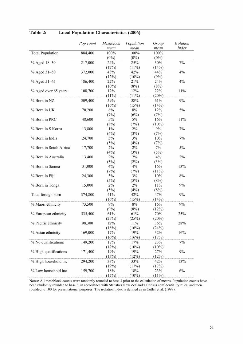
51

Table 2: Local Population Characteristics (2006) Pop count Meshblock

mean Population

mean Group mean

Isolation Index

Total Population 884,400 100% 100% 100% (0%) (0%) (0%)

% Aged 18–30 217,000 24% 25% 30% 7% (12%) (11%) (14%) % Aged 31–50 372,000 43% 42% 44% 4% (12%) (10%) (9%) % Aged 51–65 186,400 22% 21% 24% 4% (10%) (8%) (8%) % Aged over 65 years 108,700 12% 12% 22% 11%

(11%) (11%) (20%) % Born in NZ 509,400 59% 58% 61% 9%

(16%) (15%) (14%) % Born in UK 70,200 8% 8% 12% 5% (7%) (6%) (7%) % Born in PRC 48,600 5% 5% 16% 11% (8%) (7%) (10%) % Born in S.Korea 13,800 1% 2% 9% 7% (4%) (3%) (7%) % Born in India 24,700 3% 3% 10% 7% (5%) (4%) (7%) % Born in South Africa 17,700 2% 2% 7% 5% (4%) (3%) (5%) % Born in Australia 13,400 2% 2% 4% 2% (3%) (2%) (3%) % Born in Samoa 31,000 4% 4% 16% 13% (7%) (7%) (11%) % Born in Fiji 24,300 3% 3% 10% 8% (5%) (5%) (8%) % Born in Tonga 15,000 2% 2% 11% 9% (5%) (4%) (8%) Total foreign born 374,800 41% 42% 47% 9% (16%) (15%) (14%) % Maori ethnicity 73,500 9% 8% 16% 9%

(9%) (8%) (12%) % European ethnicity 535,400 61% 61% 70% 25%

(25%) (25%) (20%) % Pacific ethnicity 98,300 12% 11% 36% 28%

(18%) (16%) (24%) % Asian ethnicity 169,000 17% 19% 32% 16%

(16%) (16%) (17%) % No qualifications 149,200 17% 17% 23% 7%

(12%) (10%) (10%) % High qualifications 171,400 19% 19% 27% 9%

(13%) (12%) (12%) % High household inc 294,200 33% 33% 42% 13%

(19%) (17%) (17%) % Low household inc 159,700 18% 18% 23% 6%

(12%) (10%) (11%) Notes: All meshblock counts were randomly rounded to base 3 prior to the calculation of means. Population counts have been randomly rounded to base 3, in accordance with Statistics New Zealand’s Census confidentiality rules, and then rounded to 100 for presentational purposes. The isolation index is defined as in Cutler et al. (1999).

52

Table 3: Land-price regressions

Bivariate regressions

Log of land price per hectare

Log of land price per hectare

Log of land price per hectare

Log of land price per hectare

(1) (2) (3) (4) (5) log of neighbourhood land price 0.942** 0.656** 0.370** 0.371** (0.006) (0.013) (0.011) (0.012) time lag of land price (logged) 0.857** 0.510** 0.522**

(0.005) (0.010) (0.009) log of population 0.056** 0.258** 0.199** 0.097** 0.063** (0.015) (0.012) (0.010) (0.008) (0.007) log of percent new 0.696** 0.172** 0.167** 0.094** 0.103** (0.031) (0.022) (0.020) (0.015) (0.013) -1*(log of land area) 0.567** 0.530** 0.388** 0.168** 0.146** (0.009) (0.010) (0.010) (0.008) (0.008) Year dummy: 2006 0.661** 0.533** 0.197** 0.145** 0.143** (0.016) (0.011) (0.011) (0.009) (0.010) Near school 0.297** 0.008 -0.031** -0.022** -0.021** (0.016) (0.007) (0.007) (0.005) (0.005) Near supermarket 0.484** -0.031** -0.062** -0.047** -0.048** (0.014) (0.010) (0.009) (0.007) (0.007) Near railway station 0.093** -0.085** -0.007 0.001 0 (0.010) (0.007) (0.006) (0.005) (0.005) Near bank 0.640** 0.100** 0.081** 0.026** 0.022** (0.012) (0.010) (0.009) (0.007) (0.007) Near airport -0.246** -0.119** -0.030* -0.005 0.007 (0.019) (0.017) (0.015) (0.012) (0.012) Near CBD 0.979** 0.360** 0.037* -0.017 -0.007 (0.010) (0.015) (0.016) (0.012) (0.012) Near coast 0.102** 0.081** 0.027** 0.003 0.003 (0.008) (0.005) (0.004) (0.004) (0.003) Near motorway ramp 0.263** -0.055** -0.003 0.003 0.004 (0.010) (0.007) (0.006) (0.005) (0.005) % renting 0.338** 0.433** 0.137** 0.117** 0.116** (0.048) (0.052) (0.047) (0.034) (0.036) % of detached dwellings -1.394** -0.116** -0.110** -0.025 -0.004 (0.040) (0.034) (0.031) (0.023) (0.022) log of median HH income 1.116** 0.393** 0.250** 0.130** 0.080** (0.027) (0.037) (0.032) (0.023) (0.023) log of employment 0.104** 0.096** 0.089** 0.035** 0.029** (0.006) (0.005) (0.005) (0.004) (0.004) log of neighbourhood empl 0.537** 0.118** -0.066** -0.016* -0.016* (0.008) (0.009) (0.009) (0.007) (0.007) % Maori ethnicity -3.463** -0.123 -0.232** -0.113 -0.085 (0.098) (0.098) (0.090) (0.064) (0.072) % other ethnicity 2.898** 0.166 -0.269 -0.214 0.16 (0.377) (0.246) (0.222) (0.184) (0.255) % Pacific ethnicity -1.492** -0.131 -0.005 0.183* 0.248** (0.033) (0.113) (0.100) (0.081) (0.080) % Asian ethnicity 1.084** 0.832** 0.643** 0.268** 0.282** (0.056) (0.154) (0.135) (0.101) (0.085)

(continued)

53

Table 3 (continued) Bivariate

regressions Log of land price per hectare

Log of land price per hectare

Log of land price per hectare

Log of land price per hectare

(1) (2) (3) (4) (5) % Born in UK 1.217** -0.606** -0.583** -0.371** -0.219** (0.135) (0.118) (0.103) (0.075) (0.068) % Born in PRC 2.161** -1.438** -1.196** -0.600** -0.455** (0.127) (0.200) (0.174) (0.130) (0.133) % Born in Korea 4.364** -0.525 -0.199 -0.414* -0.728** (0.315) (0.274) (0.248) (0.183) (0.189) % Born in India 1.260** -0.826** -0.688** -0.062 -0.131 (0.177) (0.222) (0.198) (0.139) (0.181) % Born in South Africa 1.921** -0.135 -0.746** -0.590** -0.085 (0.257) (0.218) (0.194) (0.145) (0.290) % Born in Australia 6.640** 0.239 0.206 0.219 0.018 (0.916) (0.316) (0.346) (0.173) (0.211) % Born in Samoa -3.507** -0.346* -0.286 -0.320* -0.319* (0.081) (0.175) (0.157) (0.129) (0.126) % Born in Fiji -2.545** -1.274** -0.857** -0.244 -0.242 (0.178) (0.229) (0.199) (0.151) (0.132) % Born in Tonga -3.303** -0.007 -0.111 -0.155 -0.444** (0.174) (0.200) (0.171) (0.138) (0.164) % Born other countries 1.924** -0.420** -0.368** -0.291** -0.395** (0.122) (0.137) (0.123) (0.091) (0.077) % Aged 18–30 0.512** -1.178** -0.731** -0.370** -0.240** (0.099) (0.104) (0.093) (0.068) (0.066) % Aged 31–50 -1.169** -0.731** -0.435** -0.110* -0.077 (0.093) (0.084) (0.075) (0.052) (0.054) % Aged over 65 years 1.173** 0.409** 0.079 0.088 0.173** (0.089) (0.101) (0.088) (0.065) (0.064) % High qualifications 4.774** 0.693** 0.04 0.051 0.117 (0.055) (0.085) (0.079) (0.059) (0.062) % No qualifications -4.167** -0.704** -0.232** -0.115 -0.013 (0.084) (0.096) (0.084) (0.061) (0.051) Intercept 7.199** 1.265** -0.057 0.485 (0.468) (0.406) (0.290) (0.294) Adj R-sq 0.729 0.788 0.859 0.857 Meshblock Count 16216 16216 16216 16216 Note: All regressions contain a constant, a year dummy for 2001, and a dummy variable for meshblocks in which all residents have been present for at least 5 years (percent new = 0). Standard errors in parentheses. Significance indicators: 1% (**); 5% (*). Column 5 contains lagged values of area composition variables.

54

Table 4: Profiles of entrant subgroups (2006) Qualifications Age Household structure 2006 Census % with

no qual % with degree

% 18–30 years

% 31–50 years

% empl FT % renting % couples with dep

% single with dep

% couple - no dep

% single - no dep

Median HH inc

Usually resident pop 884,400 17% 9% 25% 42% 51% 30% 28% 6% 34% 32% $43,000 All entrants 246,600 9% 23% 34% 46% 44% 40% 25% 4% 26% 44% $40,000 Entrants by ethnicity European 99,300 9% 31% 30% 49% 63% 43% 25% 3% 35% 36% $54,600 Maori 14,900 29% 10% 42% 43% 52% 59% 20% 14% 20% 45% $38,800 Pacific 17,800 25% 5% 36% 43% 45% 56% 37% 11% 18% 34% $31,400 Asian 75,800 7% 31% 41% 45% 41% 43% 34% 4% 30% 32% $27,400 Entrants by qualification Degree qualified 56,800 0% 100% 31% 59% 68% 47% 34% 2% 34% 29% $50,500 No qualification 22,700 100% 0% 24% 38% 37% 47% 22% 9% 29% 40% $29,100 Entrants by household income High household income 68,600 5% 37% 34% 49% 67% 36% 20% 1% 39% 40% $76,300 Low household income 47,900 15% 17% 39% 40% 22% 54% 30% 10% 23% 38% $12,300 Entrants overseas 5 years earlier Born in Australia 2,600 3% 37% 37% 54% 68% 54% 29% 2% 40% 29% $64,000 Born in NZ 18,600 7% 39% 24% 65% 69% 37% 28% 4% 34% 34% $62,500 Born in UK 11,100 3% 41% 20% 65% 68% 43% 37% 1% 39% 22% $57,500 Born in South Africa 7,400 1% 21% 25% 59% 68% 55% 50% 3% 33% 15% $50,500 Born in India 14,000 3% 59% 30% 58% 63% 54% 51% 2% 29% 19% $35,400 Born in other countries 30,400 8% 32% 37% 50% 47% 53% 35% 4% 29% 33% $35,000 Born in Fiji 8,000 9% 12% 39% 44% 55% 41% 44% 3% 35% 19% $33,800 Born in Samoa 3,600 20% 3% 39% 45% 39% 62% 44% 9% 14% 33% $26,400 Born in Tonga 2,000 28% 5% 36% 42% 39% 60% 38% 8% 18% 37% $26,300 Born in PRC 24,100 7% 24% 57% 31% 25% 40% 18% 3% 34% 45% $19,600 Born in South Korea 6,000 6% 15% 29% 61% 27% 42% 45% 13% 17% 24% $17,100 Total: Born overseas 109,200 7% 30% 38% 49% 47% 48% 36% 4% 30% 30% $33,200

Notes: Population counts have been randomly rounded to base 3, in accordance with Statistics New Zealand’s Census confidentiality rules, and then rounded to 100 for presentation. Entrants are defined as residents of the Auckland Urban Area who were living outside the Auckland Region five years earlier. Statistics in this table are for all meshblocks in the Auckland Urban Area (i.e.: it includes meshblocks that are excluded from subsequent regression analysis because of missing values of key variables).

55

Table 5: Location choice Negative binomial regression. Dependent variable = number of entrants in a meshblock

Entered Akld region Entered Akld region

Recent migrant entrant

Return NZer entrant

High H'hold Income entrant

Low H'hold Income entrant

High qual entrant

Low qual entrant

log of land price per hectare -0.015* -0.033** 0.057** 0.080** -0.087** 0.071** -0.167** (0.006) (0.009) (0.014) (0.017) (0.013) (0.010) (0.014) log of population 1 1 1 1 1 1 1 (na) (na) (na) (na) (na) (na) (na) Unobserved amenities 0.080** 0.169** 0.306** 0.269** 0.061** 0.470** -0.240** (0.007) (0.010) (0.016) (0.021) (0.014) (0.012) (0.016) log of percent new 0.701** 1.378** 0.683** 0.885** 1.081** 1.357** 0.501** (0.022) (0.020) (0.030) (0.088) (0.028) (0.023) (0.029) Dispersion parameter: ln() -2.588** -1.269** -1.103** -0.999** -0.669** -1.510** -0.871** (0.032) (0.017) (0.033) (0.046) (0.018) (0.028) (0.024) Pseudo R-sq 0.044 0.054 0.044 0.055 0.021 0.11 0.031 Dispersion () 0.075 0.281 0.332 0.368 0.512 0.221 0.418 Log likelihood -5.58E+04 -4.85E+04 -2.78E+04 -4.30E+04 -4.14E+04 -3.77E+04 -3.10E+04 Meshblock count 16,216 16,216 16,216 16,216 16,216 16,216 16,216 Instrumental Variables Estimates log of land price per hectare -0.072** -0.014 0.01 0.108** -0.099** 0.073** -0.239** (0.010) (0.014) (0.023) -0.025 (0.020) (0.017) (0.021) log of population 1 1 1 1 1 1 1 (na) (na) (na) (na) (na) (na) (na) Unobserved amenities 0.116** 0.149** 0.335** 0.226** 0.069** 0.443** -0.154** (0.009) (0.014) (0.023) -0.025 (0.019) (0.017) (0.021) log of percent new 1.075** 1.495** 0.887** 1.343** 1.175** 1.934** 0.082 (0.025) (0.042) (0.064) -0.064 (0.058) (0.048) (0.059) Dispersion parameter: ln() -2.627** -1.277** -1.148** -1.030** -0.670** -1.563** -0.910** (0.028) (0.017) (0.034) -0.037 (0.018) (0.029) (0.025) Pseudo R-sq 0.048 0.055 0.046 0.058 0.021 0.114 0.035 Dispersion () 0.072 0.279 0.317 0.357 0.512 0.21 0.403 Log likelihood -5.55E+04 -4.84E+04 -2.77E+04 -4.28E+04 -4.14E+04 -3.75E+04 -3.09E+04 Meshblock count 16,216 16,216 16,216 16,216 16,216 16,216 16,216 Note: All regressions contain a constant, a year dummy for 2001, and a dummy variable for meshblocks in which all residents have been present for at least five years (percent new = 0). Standard errors in parentheses. Significance indicators: 1% (**); 5% (*)

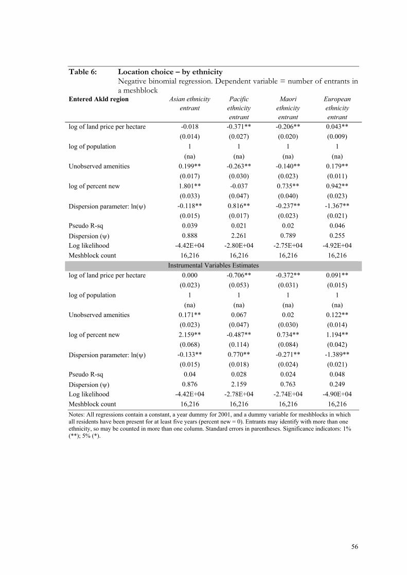
56

Table 6: Location choice – by ethnicity Negative binomial regression. Dependent variable = number of entrants in a meshblock

Entered Akld region Asian ethnicity entrant

Pacific ethnicity entrant

Maori ethnicity entrant

European ethnicity entrant

log of land price per hectare -0.018 -0.371** -0.206** 0.043**

(0.014) (0.027) (0.020) (0.009)

log of population 1 1 1 1

(na) (na) (na) (na)

Unobserved amenities 0.199** -0.263** -0.140** 0.179**

(0.017) (0.030) (0.023) (0.011)

log of percent new 1.801** -0.037 0.735** 0.942**

(0.033) (0.047) (0.040) (0.023)

Dispersion parameter: ln() -0.118** 0.816** -0.237** -1.367**

(0.015) (0.017) (0.023) (0.021)

Pseudo R-sq 0.039 0.021 0.02 0.046

Dispersion () 0.888 2.261 0.789 0.255

Log likelihood -4.42E+04 -2.80E+04 -2.75E+04 -4.92E+04

Meshblock count 16,216 16,216 16,216 16,216

Instrumental Variables Estimates

log of land price per hectare 0.000 -0.706** -0.372** 0.091**

(0.023) (0.053) (0.031) (0.015)

log of population 1 1 1 1

(na) (na) (na) (na)

Unobserved amenities 0.171** 0.067 0.02 0.122**

(0.023) (0.047) (0.030) (0.014)

log of percent new 2.159** -0.487** 0.734** 1.194**

(0.068) (0.114) (0.084) (0.042)

Dispersion parameter: ln() -0.133** 0.770** -0.271** -1.389**

(0.015) (0.018) (0.024) (0.021)

Pseudo R-sq 0.04 0.028 0.024 0.048

Dispersion () 0.876 2.159 0.763 0.249

Log likelihood -4.42E+04 -2.78E+04 -2.74E+04 -4.90E+04

Meshblock count 16,216 16,216 16,216 16,216

Notes: All regressions contain a constant, a year dummy for 2001, and a dummy variable for meshblocks in which all residents have been present for at least five years (percent new = 0). Entrants may identify with more than one ethnicity, so may be counted in more than one column. Standard errors in parentheses. Significance indicators: 1% (**); 5% (*).

57

Table 7: Location choice – by country of birth Negative binomial regression. Dependent variable = number of entrants in a meshblock

Entered Akld region Recent entrant born in S. Korea PRC Tonga Samoa Fiji India S. Africa UK Australia log of land price per hectare 0.122** -0.173** -0.471** -0.452** ‐0.169** -0.01 0.013 0.088** 0.175** (0.035) (0.025) (0.054) (0.050) (0.037) (0.034) (0.029) (0.023) (0.035) log of population 1 1 1 1 1 1 1 1 1 (na) (na) (na) (na) (na) (na) (na) (na) (na) Unobserved amenities 0.162** 0.605** -0.105 -0.578** ‐0.619** 0.101** 0.082* 0.181** 0.324** (0.041) (0.030) (0.061) (0.052) (0.043) (0.037) (0.033) (0.026) (0.042) log of percent new 1.929** 2.051** -0.127 -0.059 1.539** 2.265** 1.313** 0.785** 0.948** (0.082) (0.058) (0.095) (0.082) (0.087) (0.083) (0.069) (0.048) (0.077) Dispersion parameter: ln() 1.511** 0.894** 2.127** 1.771** 1.588** 1.385** 1.261** 0.249** 0.160* (0.029) (0.019) (0.035) (0.029) (0.024) (0.023) (0.024) (0.027) (0.063) Pseudo R-sq 0.029 0.036 0.016 0.036 0.03 0.034 0.011 0.022 0.04 Dispersion () 4.531 2.446 8.39 5.874 4.896 3.993 3.531 1.282 1.173 Log likelihood -1.31E+04 -2.66E+04 -8742.176 -1.15E+04 ‐1.53E+04 -1.86E+04 -1.71E+04 -2.13E+04 -9981.824 Meshblock count 16,216 16,216 16,216 16,216 16,216 16,216 16,216 16,216 16,216 Instrumental Variables Estimateslog of land price per ha 0.383** -0.169** -0.962** ‐0.865** -0.338** ‐0.173** 0.296** 0.235** 0.240** (0.063) (0.042) (0.086) (0.083) (0.061) (0.053) (0.056) (0.039) (0.059) log of population 1 1 1 1 1 1 1 1 1 (na) (na) (na) (na) (na) (na) (na) (na) (na) Unobserved amenities -0.085 0.593** 0.361** -0.183* -0.464** 0.228** -0.161** 0.048 0.235** (0.058) (0.042) (0.081) (0.074) (0.060) (0.052) (0.052) (0.037) (0.057) log of percent new 2.402** 2.409** -0.579** -0.801** 1.190** 2.881** 1.191** 0.719** 1.411** (0.170) (0.124) (0.207) (0.179) (0.170) (0.173) (0.146) (0.102) (0.162) Dispersion parameter: ln() 1.465** 0.887** 2.070** 1.715** 1.575** 1.357** 1.246** 0.240** 0.135* (0.030) (0.019) (0.035) (0.030) (0.025) (0.024) (0.025) (0.027) (0.064) Pseudo R-sq 0.035 0.037 0.023 0.044 0.032 0.038 0.013 0.023 0.043 Dispersion () 4.329 2.428 7.921 5.555 4.832 3.884 3.477 1.271 1.144 Log likelihood -1.30E+04 -2.66E+04 -8677.66 -1.14E+04 ‐1.52E+04 -1.86E+04 -1.71E+04 -2.13E+04 -9958.214 Meshblock count 16,216 16,216 16,216 16,216 16,216 16,216 16,216 16,216 16,216

Note: All regressions contain a constant, a year dummy for 2001, and a dummy variable for meshblocks in which all residents have been present for at least five years (percent new = 0). Standard errors in parentheses. Significance indicators: 1% (**); 5% (*)

58

Table 8: Location choice (with amenities) Negative binomial regression. Dependent variable = number of entrants in a meshblock

Entered Akld

region

Recent migrant entrant

Return NZer

entrant

High HH income entrant

Low HH income entrant

High qual entrant

Low qual entrant

Entered Akld region IV IV IV IV IV IV IV log of land price/ ha -0.020* 0.058** 0.012 0.011 0.070** 0.036** 0.016 (0.008) (0.011) (0.023) (0.020) (0.018) (0.013) (0.018) log of population 1 1 1 1 1 1 1 (na) (na) (na) (na) (na) (na) (na) Unobserved amenities 0.012 0.026 0.031 0.015 -0.055* 0.032 -0.002 (0.010) (0.015) (0.027) (0.022) (0.022) (0.017) (0.024) log of percent new 0.561** 0.206** 0.535** 0.739** 0.303** 0.410** 0.159 (0.045) (0.062) (0.137) (0.110) (0.100) (0.079) (0.112) Near school 0.003 0.022** -0.01 0.007 0.013 0.007 0.006 (0.004) (0.005) (0.011) (0.008) (0.009) (0.006) (0.009) Near supermarket -0.002 0.024** 0.005 -0.013 0.019 0.017* 0.030* (0.005) (0.007) (0.014) (0.011) (0.011) (0.008) (0.012) Near railway station 0.002 0.024** -0.045** -0.016 0.022* 0.026** -0.008 (0.004) (0.006) (0.012) (0.010) (0.009) (0.007) (0.010) Near bank 0 0.011 0.033* -0.011 0.003 -0.003 0.007 (0.005) (0.007) (0.014) (0.012) (0.011) (0.008) (0.013) Near airport -0.052** 0.073** 0.142** 0.174** -0.058* 0.006 -0.084** (0.013) (0.019) (0.037) (0.030) (0.027) (0.024) (0.029) Near CBD 0.063** 0.027 0.081* 0.013 -0.097** 0.064** -0.140** (0.012) (0.017) (0.033) (0.026) (0.028) (0.020) (0.031) Near coast 0.003 -0.002 0.004 0.012 0.011 0.01 0.018* (0.003) (0.004) (0.009) (0.007) (0.007) (0.005) (0.007) Near motorway ramp -0.016** -0.007 -0.004 0.027** 0.002 -0.008 0.003 (0.004) (0.006) (0.012) (0.009) (0.009) (0.007) (0.010) log of neighb empl -0.004 0.012 -0.001 -0.016 -0.026* 0.013 -0.016 (0.005) (0.008) (0.015) (0.013) (0.012) (0.009) (0.013) -1*(log of land area) 0.020** 0.002 0.022 0.016 -0.026 0.019* -0.034* (0.006) (0.008) (0.017) (0.014) (0.014) (0.010) (0.014) % renting 0.187* 0.204* 0.577** -0.691** 0.303 0.550** 0.084 (0.075) (0.099) (0.221) (0.201) (0.156) (0.121) (0.173) % detached dwellings -0.205** -0.424** 0.189* -0.163* -0.425** -0.109* -0.448** (0.028) (0.040) (0.084) (0.071) (0.063) (0.047) (0.074) log of median HH inc -0.053 -0.127 -0.005 0.963** -1.173** -0.013 0.08 (0.072) (0.088) (0.186) (0.166) (0.137) (0.102) (0.176) log of employment 0.015** -0.005 -0.011 0.032** -0.016* -0.008 0.008 (0.003) (0.005) (0.010) (0.008) (0.007) (0.006) (0.008) % Asian ethnicity -0.550** -0.23 -1.071 -0.378 0.958* 0.125 0.948* (0.186) (0.271) (0.581) (0.440) (0.420) (0.302) (0.467) % Pacific ethnicity -0.567** -1.306** -0.32 -0.54 -0.151 -0.04 -0.175 (0.153) (0.209) (0.450) (0.384) (0.323) (0.275) (0.329) % Maori ethnicity 0.788** -0.768** -0.534 0.423 0.461 -1.090** 1.063** (0.136) (0.171) (0.378) (0.335) (0.256) (0.220) (0.273) % other ethnicity -0.179 1.696 -1.335 2.113 0.834 4.185** 2.611 (0.727) (1.108) (2.533) (1.875) (1.750) (1.276) (2.150)

(continued)

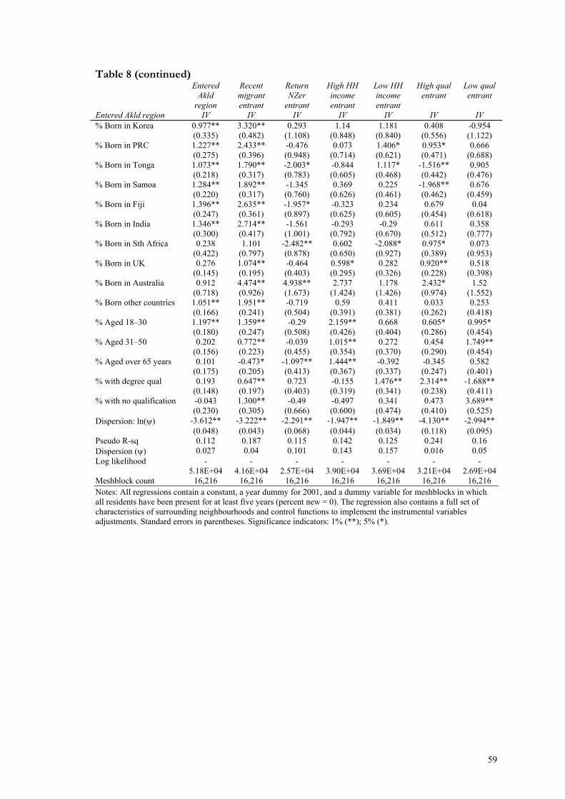
59

Table 8 (continued) Entered

Akld region

Recent migrant entrant

Return NZer

entrant

High HH income entrant

Low HH income entrant

High qual entrant

Low qual entrant

Entered Akld region IV IV IV IV IV IV IV % Born in Korea 0.977** 3.320** 0.293 1.14 1.181 0.408 -0.954 (0.335) (0.482) (1.108) (0.848) (0.840) (0.556) (1.122) % Born in PRC 1.227** 2.433** -0.476 0.073 1.406* 0.953* 0.666 (0.275) (0.396) (0.948) (0.714) (0.621) (0.471) (0.688) % Born in Tonga 1.073** 1.790** -2.003* -0.844 1.117* -1.516** 0.905 (0.218) (0.317) (0.783) (0.605) (0.468) (0.442) (0.476) % Born in Samoa 1.284** 1.892** -1.345 0.369 0.225 -1.968** 0.676 (0.220) (0.317) (0.760) (0.626) (0.461) (0.462) (0.459) % Born in Fiji 1.396** 2.635** -1.957* -0.323 0.234 0.679 0.04 (0.247) (0.361) (0.897) (0.625) (0.605) (0.454) (0.618) % Born in India 1.346** 2.714** -1.561 -0.293 -0.29 0.611 0.358 (0.300) (0.417) (1.001) (0.792) (0.670) (0.512) (0.777) % Born in Sth Africa 0.238 1.101 -2.482** 0.602 -2.088* 0.975* 0.073 (0.422) (0.797) (0.878) (0.650) (0.927) (0.389) (0.953) % Born in UK 0.276 1.074** -0.464 0.598* 0.282 0.920** 0.518 (0.145) (0.195) (0.403) (0.295) (0.326) (0.228) (0.398) % Born in Australia 0.912 4.474** 4.938** 2.737 1.178 2.432* 1.52 (0.718) (0.926) (1.673) (1.424) (1.426) (0.974) (1.552) % Born other countries 1.051** 1.951** -0.719 0.59 0.411 0.033 0.253 (0.166) (0.241) (0.504) (0.391) (0.381) (0.262) (0.418) % Aged 18–30 1.197** 1.359** -0.29 2.159** 0.668 0.605* 0.995* (0.180) (0.247) (0.508) (0.426) (0.404) (0.286) (0.454) % Aged 31–50 0.202 0.772** -0.039 1.015** 0.272 0.454 1.749** (0.156) (0.223) (0.455) (0.354) (0.370) (0.290) (0.454) % Aged over 65 years 0.101 -0.473* -1.097** 1.444** -0.392 -0.345 0.582 (0.175) (0.205) (0.413) (0.367) (0.337) (0.247) (0.401) % with degree qual 0.193 0.647** 0.723 -0.155 1.476** 2.314** -1.688** (0.148) (0.197) (0.403) (0.319) (0.341) (0.238) (0.411) % with no qualification -0.043 1.300** -0.49 -0.497 0.341 0.473 3.689** (0.230) (0.305) (0.666) (0.600) (0.474) (0.410) (0.525) Dispersion: ln() -3.612** -3.222** -2.291** -1.947** -1.849** -4.130** -2.994** (0.048) (0.043) (0.068) (0.044) (0.034) (0.118) (0.095) Pseudo R-sq 0.112 0.187 0.115 0.142 0.125 0.241 0.16 Dispersion () 0.027 0.04 0.101 0.143 0.157 0.016 0.05 Log likelihood -

5.18E+04 -

4.16E+04 -

2.57E+04 -

3.90E+04 -

3.69E+04 -

3.21E+04 -

2.69E+04 Meshblock count 16,216 16,216 16,216 16,216 16,216 16,216 16,216 Notes: All regressions contain a constant, a year dummy for 2001, and a dummy variable for meshblocks in which all residents have been present for at least five years (percent new = 0). The regression also contains a full set of characteristics of surrounding neighbourhoods and control functions to implement the instrumental variables adjustments. Standard errors in parentheses. Significance indicators: 1% (**); 5% (*).

60

Table 9: Location choice (with amenities): by ethnicity Negative binomial regression. Dependent variable = number of entrants in a meshblock

Asian ethnicity entrant

Pacific ethnicity entrant

Maori ethnicity entrant

European ethnicity entrant

Entered Akld region IV IV IV IV log of land price per hectare 0.052** -0.108** -0.076** 0.008 (0.017) (0.032) (0.024) (0.011) log of population 1 1 1 1 (na) (na) (na) (na) Unobserved amenities 0.031 0.122** 0.016 0.018 (0.022) (0.042) (0.032) (0.012) log of percent new -0.006 0.851** 0.644** 0.758** (0.092) (0.197) (0.141) (0.065) Near school 0.029** 0.01 -0.004 0.002 (0.008) (0.015) (0.012) (0.005) Near supermarket 0.080** 0.028 0.034* 0.000 (0.010) (0.017) (0.015) (0.007) Near railway station 0.057** 0.025 -0.02 -0.002 (0.008) (0.015) (0.012) (0.006) Near bank -0.017 -0.014 -0.015 -0.018** (0.010) (0.018) (0.016) (0.007) Near airport 0.195** -0.013 0.012 -0.027 (0.028) (0.045) (0.038) (0.018) Near CBD 0.009 0.557** 0.144** -0.016 (0.026) (0.061) (0.043) (0.015) Near coast 0.001 0.01 0.042** 0.014** (0.006) (0.011) (0.009) (0.004) Near motorway ramp 0.012 0.018 0.061** 0.001 (0.009) (0.015) (0.012) (0.005) log of neighbourhood empl 0.059** 0.028 0.003 -0.001 (0.012) (0.020) (0.016) (0.007) -1*(log of land area) -0.008 0.036 0.03 0.018* (0.012) (0.022) (0.019) (0.008) % renting -0.061 0.072 -0.324 -0.008 (0.151) (0.250) (0.219) (0.107) % detached dwellings -0.474** 0.153 -0.335** -0.120** (0.060) (0.117) (0.088) (0.043) log of median HH income -0.265 0.015 -0.292 0.077 (0.140) (0.242) (0.203) (0.095) log of employment -0.015* -0.005 0.017 0.012* (0.007) (0.012) (0.010) (0.005) % Asian ethnicity 2.295** -0.138 0.296 -1.170** (0.404) (0.736) (0.607) (0.266) % Pacific ethnicity -1.229** 1.793** -0.487 -0.959** (0.319) (0.485) (0.426) (0.223) % Maori ethnicity -0.994** 1.623** 2.814** -0.163 (0.269) (0.397) (0.383) (0.174) % other ethnicity 3.615* 6.716 6.414* -0.017 (1.584) (3.461) (2.694) (1.110)

(continued)

61

Table 9 (continued) Asian ethnicity

entrant Pacific

ethnicity entrant

Maori ethnicity entrant

European ethnicity entrant

Entered Akld region IV IV IV IV % Born in Korea 2.887** -2.026 -1.766 -0.319 (0.777) (1.874) (1.278) (0.464) % Born in PRC 1.534** 0.406 -2.300* -0.393 (0.593) (1.042) (0.947) (0.427) % Born in Tonga 0.279 2.105** -0.126 -1.605** (0.515) (0.659) (0.652) (0.389) % Born in Samoa -0.317 2.554** -0.233 -1.178** (0.484) (0.664) (0.610) (0.371) % Born in Fiji 1.467** 1.336 -0.964 -0.18 (0.556) (0.919) (0.823) (0.421) % Born in India 1.034 1.506 -0.291 -1.127* (0.666) (1.167) (0.961) (0.453) % Born in South Africa -1.126 -4.477 -2.736* 1.42 (0.907) (2.769) (1.295) (0.744) % Born in UK 0.683* -0.304 -0.126 0.414* (0.297) (0.595) (0.508) (0.186) % Born in Australia 6.282** 6.379* 4.196 1.697* (1.622) (2.510) (2.657) (0.806) % Born other countries 0.576 0.365 -1.150* 0.105 (0.355) (0.699) (0.515) (0.231) % Aged 18–30 2.294** 2.034* 3.609** 1.486** (0.372) (0.791) (0.553) (0.252) % Aged 31–50 1.252** 0.446 1.167* 0.607** (0.360) (0.776) (0.534) (0.227) % Aged over 65 years -0.01 0.289 0.221 0.609* (0.306) (0.701) (0.473) (0.253) % with degree qualification 0.6 -1.126 1.341** 0.263 (0.306) (0.610) (0.480) (0.193) % with no qualification 2.135** 3.641** 3.337** -0.035 (0.490) (0.795) (0.696) (0.341) Dispersion parameter: ln() -2.148** -1.570** -2.238** -3.364** (0.033) (0.051) (0.070) (0.088) Pseudo R-sq 0.214 0.253 0.183 0.191 Dispersion () 0.117 0.208 0.107 0.035 Log likelihood -3.62E+04 -2.14E+04 -2.29E+04 -4.17E+04 Meshblock count 16,216 16,216 16,216 16,216 Notes: All regressions contain a constant, a year dummy for 2001, and a dummy variable for meshblocks in which all residents have been present for at least five years (percent new = 0). Entrants may identify with more than one ethnicity, so may be counted in more than one column. The regression also contains a full set of characteristics of surrounding neighbourhoods and control functions to implement the instrumental variables adjustments. Standard errors in parentheses. Significance indicators: 1% (**); 5% (*).

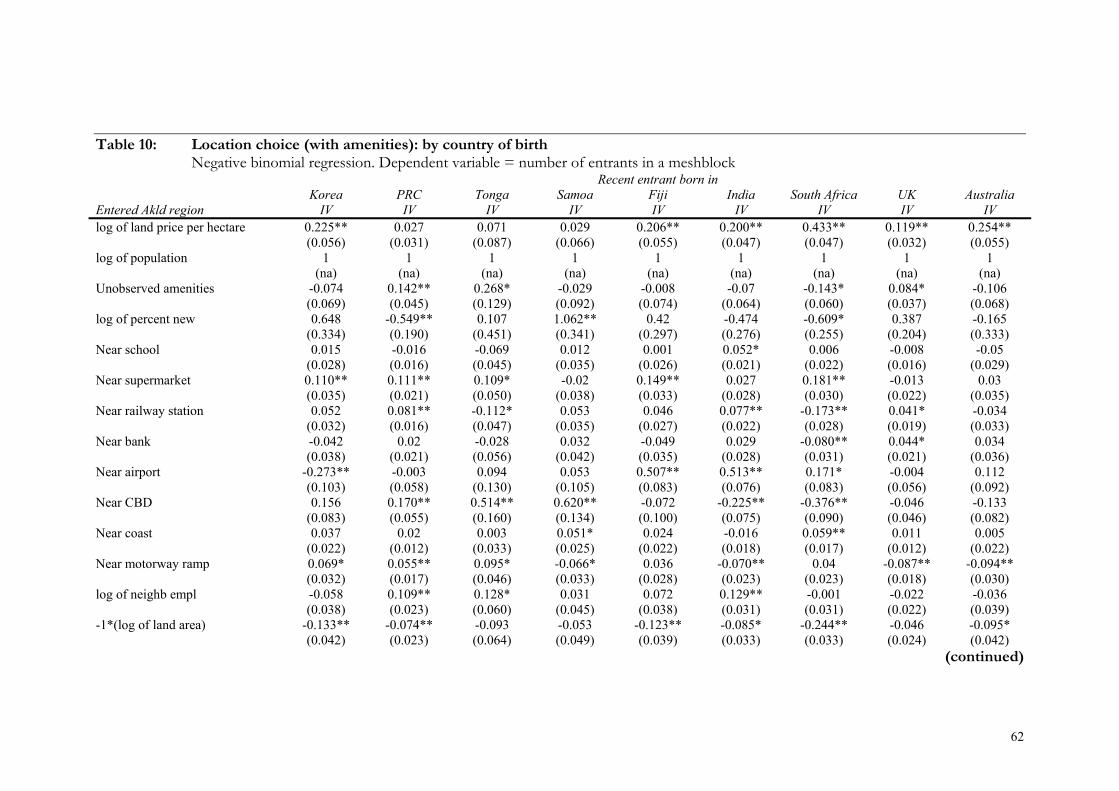
62

Table 10: Location choice (with amenities): by country of birth Negative binomial regression. Dependent variable = number of entrants in a meshblock

Recent entrant born in Korea PRC Tonga Samoa Fiji India South Africa UK Australia Entered Akld region IV IV IV IV IV IV IV IV IV log of land price per hectare 0.225** 0.027 0.071 0.029 0.206** 0.200** 0.433** 0.119** 0.254** (0.056) (0.031) (0.087) (0.066) (0.055) (0.047) (0.047) (0.032) (0.055) log of population 1 1 1 1 1 1 1 1 1 (na) (na) (na) (na) (na) (na) (na) (na) (na) Unobserved amenities -0.074 0.142** 0.268* -0.029 -0.008 -0.07 -0.143* 0.084* -0.106 (0.069) (0.045) (0.129) (0.092) (0.074) (0.064) (0.060) (0.037) (0.068) log of percent new 0.648 -0.549** 0.107 1.062** 0.42 -0.474 -0.609* 0.387 -0.165 (0.334) (0.190) (0.451) (0.341) (0.297) (0.276) (0.255) (0.204) (0.333) Near school 0.015 -0.016 -0.069 0.012 0.001 0.052* 0.006 -0.008 -0.05 (0.028) (0.016) (0.045) (0.035) (0.026) (0.021) (0.022) (0.016) (0.029) Near supermarket 0.110** 0.111** 0.109* -0.02 0.149** 0.027 0.181** -0.013 0.03 (0.035) (0.021) (0.050) (0.038) (0.033) (0.028) (0.030) (0.022) (0.035) Near railway station 0.052 0.081** -0.112* 0.053 0.046 0.077** -0.173** 0.041* -0.034 (0.032) (0.016) (0.047) (0.035) (0.027) (0.022) (0.028) (0.019) (0.033) Near bank -0.042 0.02 -0.028 0.032 -0.049 0.029 -0.080** 0.044* 0.034 (0.038) (0.021) (0.056) (0.042) (0.035) (0.028) (0.031) (0.021) (0.036) Near airport -0.273** -0.003 0.094 0.053 0.507** 0.513** 0.171* -0.004 0.112 (0.103) (0.058) (0.130) (0.105) (0.083) (0.076) (0.083) (0.056) (0.092) Near CBD 0.156 0.170** 0.514** 0.620** -0.072 -0.225** -0.376** -0.046 -0.133 (0.083) (0.055) (0.160) (0.134) (0.100) (0.075) (0.090) (0.046) (0.082) Near coast 0.037 0.02 0.003 0.051* 0.024 -0.016 0.059** 0.011 0.005 (0.022) (0.012) (0.033) (0.025) (0.022) (0.018) (0.017) (0.012) (0.022) Near motorway ramp 0.069* 0.055** 0.095* -0.066* 0.036 -0.070** 0.04 -0.087** -0.094** (0.032) (0.017) (0.046) (0.033) (0.028) (0.023) (0.023) (0.018) (0.030) log of neighb empl -0.058 0.109** 0.128* 0.031 0.072 0.129** -0.001 -0.022 -0.036 (0.038) (0.023) (0.060) (0.045) (0.038) (0.031) (0.031) (0.022) (0.039) -1*(log of land area) -0.133** -0.074** -0.093 -0.053 -0.123** -0.085* -0.244** -0.046 -0.095* (0.042) (0.023) (0.064) (0.049) (0.039) (0.033) (0.033) (0.024) (0.042)

(continued)

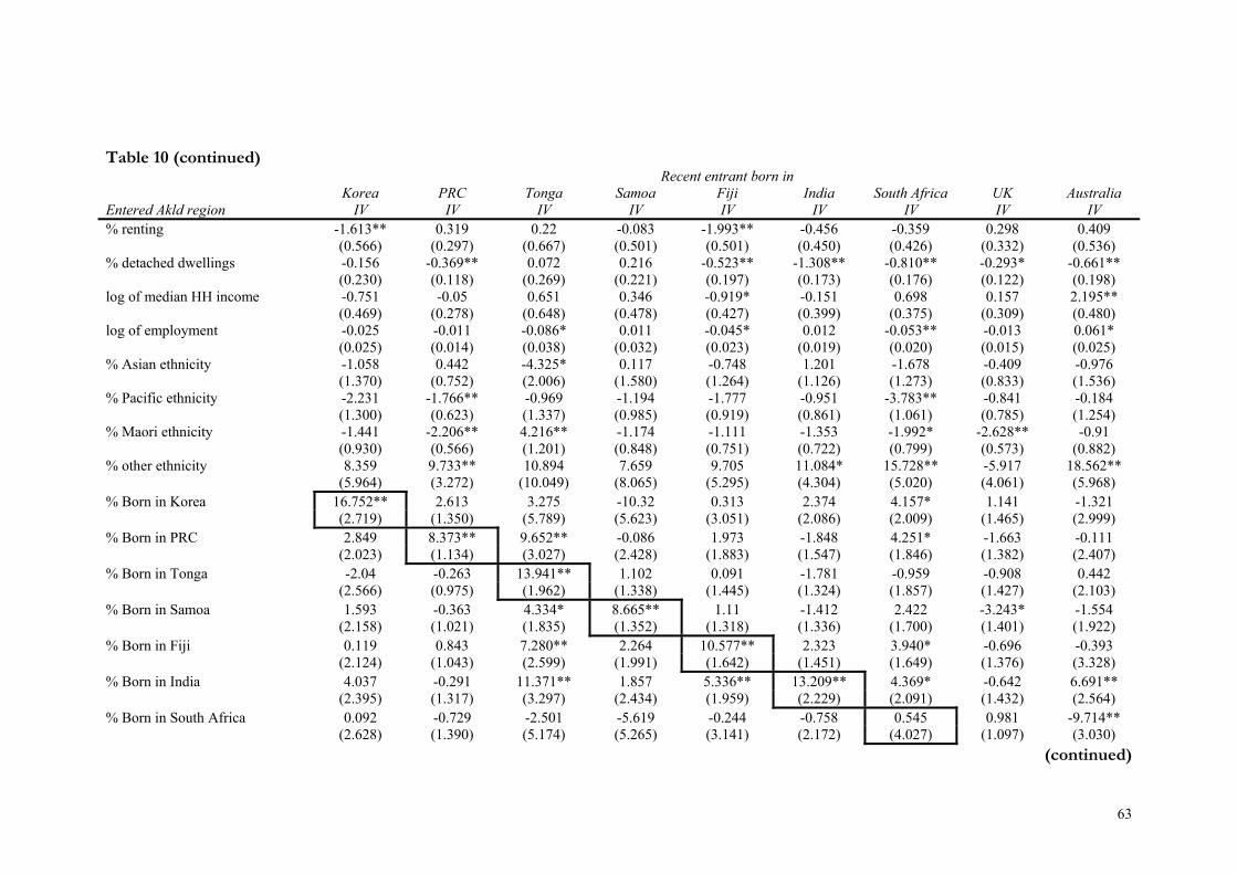
63

Table 10 (continued) Recent entrant born in Korea PRC Tonga Samoa Fiji India South Africa UK Australia Entered Akld region IV IV IV IV IV IV IV IV IV % renting -1.613** 0.319 0.22 -0.083 -1.993** -0.456 -0.359 0.298 0.409 (0.566) (0.297) (0.667) (0.501) (0.501) (0.450) (0.426) (0.332) (0.536) % detached dwellings -0.156 -0.369** 0.072 0.216 -0.523** -1.308** -0.810** -0.293* -0.661** (0.230) (0.118) (0.269) (0.221) (0.197) (0.173) (0.176) (0.122) (0.198) log of median HH income -0.751 -0.05 0.651 0.346 -0.919* -0.151 0.698 0.157 2.195** (0.469) (0.278) (0.648) (0.478) (0.427) (0.399) (0.375) (0.309) (0.480) log of employment -0.025 -0.011 -0.086* 0.011 -0.045* 0.012 -0.053** -0.013 0.061* (0.025) (0.014) (0.038) (0.032) (0.023) (0.019) (0.020) (0.015) (0.025) % Asian ethnicity -1.058 0.442 -4.325* 0.117 -0.748 1.201 -1.678 -0.409 -0.976 (1.370) (0.752) (2.006) (1.580) (1.264) (1.126) (1.273) (0.833) (1.536) % Pacific ethnicity -2.231 -1.766** -0.969 -1.194 -1.777 -0.951 -3.783** -0.841 -0.184 (1.300) (0.623) (1.337) (0.985) (0.919) (0.861) (1.061) (0.785) (1.254) % Maori ethnicity -1.441 -2.206** 4.216** -1.174 -1.111 -1.353 -1.992* -2.628** -0.91 (0.930) (0.566) (1.201) (0.848) (0.751) (0.722) (0.799) (0.573) (0.882) % other ethnicity 8.359 9.733** 10.894 7.659 9.705 11.084* 15.728** -5.917 18.562** (5.964) (3.272) (10.049) (8.065) (5.295) (4.304) (5.020) (4.061) (5.968) % Born in Korea 16.752** 2.613 3.275 -10.32 0.313 2.374 4.157* 1.141 -1.321 (2.719) (1.350) (5.789) (5.623) (3.051) (2.086) (2.009) (1.465) (2.999) % Born in PRC 2.849 8.373** 9.652** -0.086 1.973 -1.848 4.251* -1.663 -0.111 (2.023) (1.134) (3.027) (2.428) (1.883) (1.547) (1.846) (1.382) (2.407) % Born in Tonga -2.04 -0.263 13.941** 1.102 0.091 -1.781 -0.959 -0.908 0.442 (2.566) (0.975) (1.962) (1.338) (1.445) (1.324) (1.857) (1.427) (2.103) % Born in Samoa 1.593 -0.363 4.334* 8.665** 1.11 -1.412 2.422 -3.243* -1.554 (2.158) (1.021) (1.835) (1.352) (1.318) (1.336) (1.700) (1.401) (1.922) % Born in Fiji 0.119 0.843 7.280** 2.264 10.577** 2.323 3.940* -0.696 -0.393 (2.124) (1.043) (2.599) (1.991) (1.642) (1.451) (1.649) (1.376) (3.328) % Born in India 4.037 -0.291 11.371** 1.857 5.336** 13.209** 4.369* -0.642 6.691** (2.395) (1.317) (3.297) (2.434) (1.959) (2.229) (2.091) (1.432) (2.564) % Born in South Africa 0.092 -0.729 -2.501 -5.619 -0.244 -0.758 0.545 0.981 -9.714** (2.628) (1.390) (5.174) (5.265) (3.141) (2.172) (4.027) (1.097) (3.030)

(continued)

64

Table 10 (continued) Recent entrant born in Korea PRC Tonga Samoa Fiji India South Africa UK Australia Entered Akld region IV IV IV IV IV IV IV IV IV % Born in UK 2.203* 0.58 0.885 -3.104* 0.815 0.51 1.840* 1.854** 1.081 (0.957) (0.606) (1.798) (1.321) (1.028) (0.865) (0.759) (0.672) (1.031) % Born in Australia 10.569 7.546* 8.802 6.484 14.698** 16.884** 10.350** 8.314** 3.967 (6.232) (2.983) (8.403) (7.393) (4.782) (4.121) (3.975) (2.229) (5.158) % Born other countries 2.561* 0.111 3.845* 0.664 0.994 -0.311 0.076 0.792 1.118 (1.220) (0.666) (1.751) (1.317) (1.117) (0.992) (1.071) (0.699) (1.420) % Aged 18–30 3.011* 2.884** 1.623 4.113** 5.577** 6.803** 5.156** 1.153 3.599** (1.212) (0.734) (1.871) (1.422) (1.148) (1.053) (0.934) (0.701) (1.139) % Aged 31–50 0.634 2.494** 2.497 3.352* 2.893** 4.617** 4.648** 1.747* 5.131** (1.174) (0.745) (1.792) (1.510) (1.096) (1.077) (1.042) (0.720) (1.271) % Aged over 65 years -0.739 0.258 1.42 1.402 1.191 2.394** 1.809* -0.339 3.181** (1.013) (0.644) (1.512) (1.237) (0.923) (0.880) (0.825) (0.643) (1.066) % with degree qual 1.998 1.352* 0.07 -1.387 -0.472 4.059** 1.158 1.386* 2.374* (1.058) (0.583) (1.842) (1.448) (1.170) (0.933) (0.887) (0.595) (0.998) % with no qualification 3.870* 4.615** 4.044 8.104** 5.036** 7.475** 4.740** 0.952 5.130** (1.654) (0.957) (2.278) (1.818) (1.422) (1.372) (1.314) (1.055) (1.686) Dispersion ln(y) 0.028 -0.930** 0.247** -0.435** -0.129** -0.345** -0.601** -1.597** -0.833** (0.046) (0.040) (0.065) (0.068) (0.048) (0.045) (0.052) (0.069) (0.149) Pseudo R-sq 0.24 0.24 0.275 0.288 0.252 0.254 0.25 0.193 0.188 Dispersion (y) 1.028 0.395 1.28 0.647 0.879 0.709 0.548 0.203 0.435 Log likelihood -1.03E+04 -2.10E+04 -6441.96 -8458.975 -1.18E+04 -1.44E+04 -1.30E+04 -1.76E+04 -8449.56 Meshblock count 16,216 16,216 16,216 16,216 16,216 16,216 16,216 16,216 16,216 Notes: All regressions contain a constant, a year dummy for 2001, and a dummy variable for meshblocks in which all residents have been present for at least five years (percent new = 0). The regression also contains a full set of characteristics of surrounding neighbourhoods and control functions to implement the instrumental variables adjustments. Standard errors in parentheses. Significance indicators: 1% (**); 5% (*).

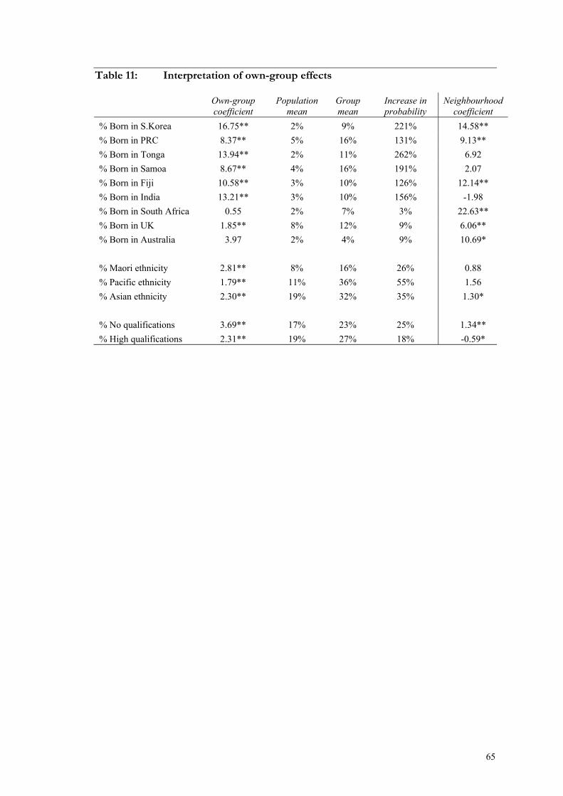
65

Table 11: Interpretation of own-group effects

Own-group coefficient

Population mean

Group mean

Increase in probability

Neighbourhood coefficient

% Born in S.Korea 16.75** 2% 9% 221% 14.58**

% Born in PRC 8.37** 5% 16% 131% 9.13**

% Born in Tonga 13.94** 2% 11% 262% 6.92

% Born in Samoa 8.67** 4% 16% 191% 2.07

% Born in Fiji 10.58** 3% 10% 126% 12.14**

% Born in India 13.21** 3% 10% 156% -1.98

% Born in South Africa 0.55 2% 7% 3% 22.63**

% Born in UK 1.85** 8% 12% 9% 6.06**

% Born in Australia 3.97 2% 4% 9% 10.69*

% Maori ethnicity 2.81** 8% 16% 26% 0.88

% Pacific ethnicity 1.79** 11% 36% 55% 1.56

% Asian ethnicity 2.30** 19% 32% 35% 1.30*

% No qualifications 3.69** 17% 23% 25% 1.34**

% High qualifications 2.31** 19% 27% 18% -0.59*

66

Figure 1 Location choice and income

(a) Number of low-income residents choosing different locations as a function of price and quality

(b) Number of middle-income residents choosing different locations as a function of price and quality