Estimating retail market potential using demographics and ...

Estimating retail market potential using

demographics and spatial analysis for home

improvement in Ontario

by

Andrei Mircea Balulescu

A thesis

presented to the University of Waterloo

in fulfillment of the

thesis requirement for the degree of

Master of Science

in

Geography

Waterloo, Ontario, Canada, 2015

© Andrei Mircea Balulescu 2015

ii

AUTHOR'S DECLARATION

I hereby declare that I am the sole author of this thesis. This is a true copy of the thesis, including any

required final revisions, as accepted by my examiners.

I understand that my thesis may be made electronically available to the public.

iii

Abstract

Alongside the breadth of literature on retail location theory, retail market assessment, and consumer

analysis, two major topics are addressed. First, a framework for estimating market demand spatially using

consumer expenditures for retail is put forward. This is a foremost step in identifying suitable locations

for retail stores, as it gives an indication into the power of the market at the location. Coupled with

reported retail sales, the approach evaluates what proportion of the market share remains for capture.

Benchmarking the aggregate estimated market expenditures against provincially reported sales reveals

that the estimation performance of one method is within one percent of the provincial sales. Spatial

analysis results for Ontario show that market demand for home improvement is clustered in Census

Metropolitan Areas, where 90% of the provincial expenditures are located. A regression analysis

identified three demographic variables as drivers of home improvement expenditures: count of

households with income over $100,000, average monthly shelter costs for owned dwellings, and count of

owned dwellings. The market demand estimation is necessary for profitability analyses, site suitability

analyses and gravity modelling. Such a framework for market demand estimation can be used by retailers

and local governments to inform policy creation for future development.

The second topic addressed by this thesis was the characterization of situational and demographic

variables contained in the service areas of home improvement chain stores. The characterization

facilitated a statistical comparison between chains to identify similarities and differences in store formats

and demographics. Results showed that big-box chains are fairly similar in their situational characteristics

and statistically significant similarities were observed when comparing the demographic variables

contained in the service areas of these chains’ stores. Chains that employ various store formats exhibit

statistically significant differences both in situational and demographic characteristics. The spatial

distribution of the chain stores was assessed using spatial statistics and showed that the chains exhibited

different spatial patterns in Ontario. Store level sales were estimated using a mathematical model that

employed store area and demographics. Future work on chain characterization using more demographic

categories would allow for the segmentation of target markets and the characterization of the landscape

for optimal retail locations.

iv

Acknowledgements

It is hard to thank those that have helped me both academically and personally during the past

two years in one short page, however, I will try my best to do so.

I would first like to thank Dr. Derek Robinson; he has been so much more than an advisor during

my master’s studies. I thank him for his patience, mentorship, leadership, kindness, and friendship as well

as setting an example worthy of following in academic, professional, and personal affairs. Dr. Robinson

has contributed most to my academic growth and to the knowledge base I have accumulated during my

studies. I thank him for mentoring me not only on the thesis, but on aspects of teaching and so many

more. Most importantly, I thank him for being a friend and sounding board for the critical moments

during my studies when everything was falling apart; his patience and trust have helped me along the way

every time. Dr. Robinson, I thank you!

It is Bogdan Caradima, close friend and colleague, whom I would like to thank second. His

company, talks, debates, discussions and most importantly moments of laughter, have made these years

pass quicker. During the most stressful moments, lunch with Bogdan was known as “a therapeutic

session”. For all the great times, good laughs, serious talks and kind friendship, Bogdan, I thank you!

My family and close friends I would like to thank third. Their encouragement and support (on all

fronts of life) have been invaluable. While listing names would entail a list longer than this letter, for all

the memories and moments, gifts, support, and help along the way, to all of you, I thank you!

While last here, she is first in all aspects; to my wife, Diana, I want to offer my utmost gratitude.

Her selfless dedication, endless support, tireless nights, continuous encouragement, and most importantly

unending love, have been the source of my drive to finish this work. Had it not been for her support along

the way, this thesis would have never seen completion. I will never find enough words to properly

describe my gratitude towards her. For putting up with me time and time again, for holding my hand

along the way, and for supporting me all this time, Diana, I thank you, I love you!

v

Dedication

I can do all things through Christ

who strengthens me.

(Philippians 4:13)

vi

Table of Contents

AUTHOR'S DECLARATION ...................................................................................................................... ii

Abstract ........................................................................................................................................................ iii

Acknowledgements ...................................................................................................................................... iv

Dedication ..................................................................................................................................................... v

Table of Contents ......................................................................................................................................... vi

List of Figures ............................................................................................................................................ viii

List of Tables ............................................................................................................................................... ix

Chapter One: Introduction ............................................................................................................................ 1

1.1 Background ......................................................................................................................................... 1

1.2 Motivations for Research .................................................................................................................... 2

1.3 The Canadian Home Improvement Market ........................................................................................ 3

1.4 Research Goals .................................................................................................................................... 3

1.5 Thesis Structure .................................................................................................................................. 4

Chapter Two: Estimating Market Demand: Expenditures ............................................................................ 6

1.0 Introduction ......................................................................................................................................... 6

2.0 Methods............................................................................................................................................... 8

2.1 Study area ........................................................................................................................................ 8

2.2 Data ............................................................................................................................................... 10

2.3 Market Demand Estimation Methods ........................................................................................... 12

2.4 Assessment of Expenditure Estimation Methods .......................................................................... 18

2.5 Spatial Analysis ............................................................................................................................ 19

3.0 Results ............................................................................................................................................... 22

3.1 Comparison of Estimation Methods.............................................................................................. 24

3.2 Spatial Analysis of Dissemination Area level Expenditures ......................................................... 27

3.3 Potential Drivers of Market Demand ............................................................................................ 32

4.0 Discussion ......................................................................................................................................... 33

4.1 Beyond Expenditures .................................................................................................................... 35

4.2 Market Demand: Key Piece in Retail Modelling .......................................................................... 36

5.0 Conclusion ........................................................................................................................................ 37

Chapter Three: Spatial Analysis of Home Improvement Chain Store Characteristics and Sales ............... 39

1.0 Introduction ....................................................................................................................................... 39

vii

2.0 Methods............................................................................................................................................. 42

2.1 Study Area .................................................................................................................................... 42

2.2 Data ............................................................................................................................................... 43

2.3 Location Theory in Literature ....................................................................................................... 44

2.4 Characterizing a Retail Chain ....................................................................................................... 46

2.5 Stores Sales Estimation ................................................................................................................. 50

3.0 Results ............................................................................................................................................... 53

3.1 Characterizing a Store ................................................................................................................... 53

3.2 Store Level Sales ........................................................................................................................... 58

4.0 Discussion ......................................................................................................................................... 60

4.1 Importance of Chain Characterization .......................................................................................... 60

4.2 Store Level Sales Proxy and Potential Modelling ......................................................................... 63

4.3 Service Area and Location Based Corrections .............................................................................. 65

5.0 Conclusion ........................................................................................................................................ 66

Chapter Four: Conclusion ........................................................................................................................... 68

1.1 Limitations ........................................................................................................................................ 68

1.2 Implication for Future Research ....................................................................................................... 69

Appendix A ................................................................................................................................................. 71

Appendix B ................................................................................................................................................. 72

Appendix C ................................................................................................................................................. 73

References ................................................................................................................................................... 76

viii

List of Figures

Figure 2.1 - Southern Ontario census subdivisions .............................................................................. 10

Figure 2.2 - Household distribution by income brackets in Ontario, 2011 .......................................... 13

Figure 2.3 - Expenditure method four displayed at the CD (a), CSD (b) and DA (c) level ................. 23

Figure 2.4 - Comparison of aggregated expenditure estimations ........................................................ 24

Figure 2.5 - Getis Ord hot spot analysis on expenditure method three at the DA level. ...................... 29

Figure 3.1 - Home Depot service area in Kitchener, Ontario, overlaid with the DAs. ........................ 47

Figure 3.2 – Five major Ontario home improvement chain ellipses. ................................................... 58

Figure 3.3 - Ontario CSDs rendered by aggregate home improvement store level sales estimates ..... 59

ix

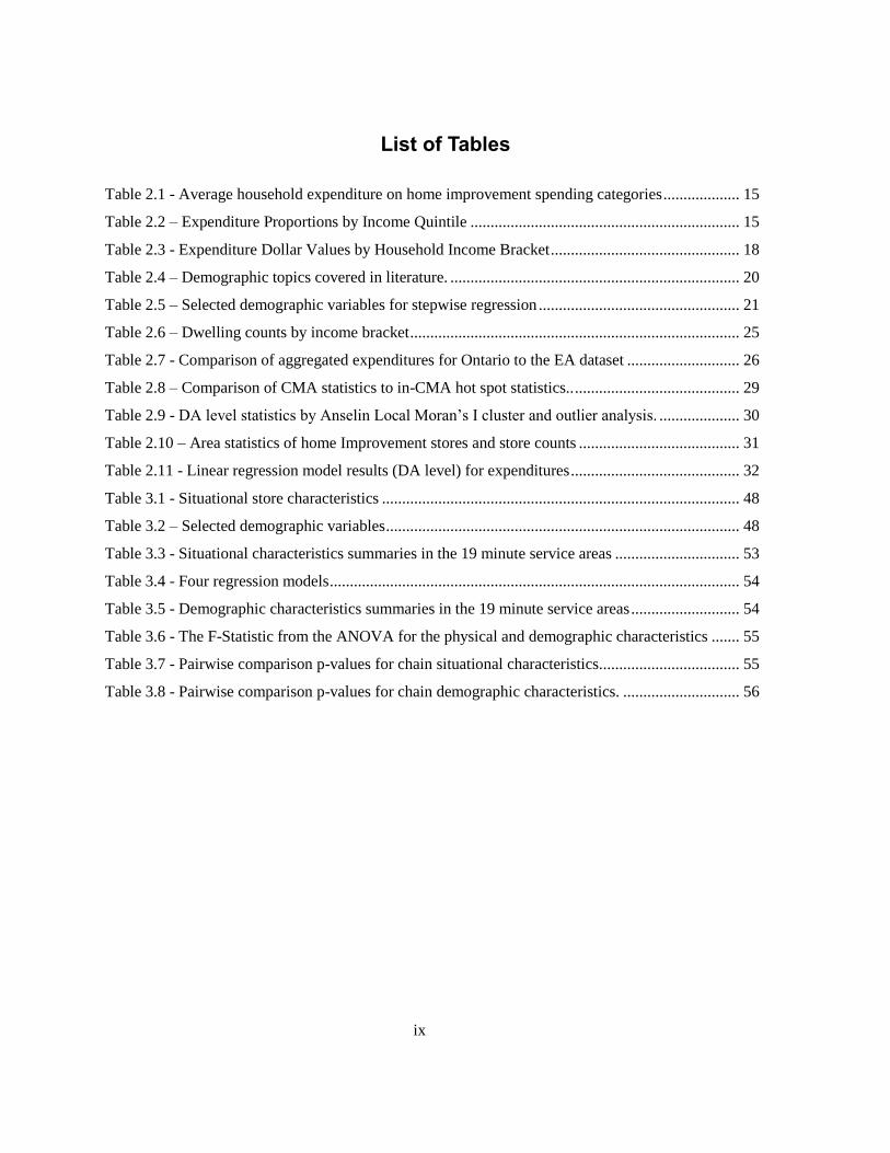
List of Tables

Table 2.1 - Average household expenditure on home improvement spending categories ................... 15

Table 2.2 – Expenditure Proportions by Income Quintile ................................................................... 15

Table 2.3 - Expenditure Dollar Values by Household Income Bracket ............................................... 18

Table 2.4 – Demographic topics covered in literature. ........................................................................ 20

Table 2.5 – Selected demographic variables for stepwise regression .................................................. 21

Table 2.6 – Dwelling counts by income bracket .................................................................................. 25

Table 2.7 - Comparison of aggregated expenditures for Ontario to the EA dataset ............................ 26

Table 2.8 – Comparison of CMA statistics to in-CMA hot spot statistics.. ......................................... 29

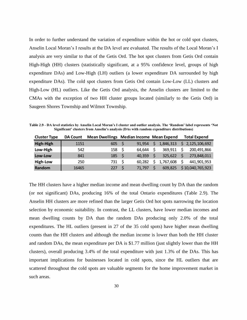
Table 2.9 - DA level statistics by Anselin Local Moran’s I cluster and outlier analysis. .................... 30

Table 2.10 – Area statistics of home Improvement stores and store counts ........................................ 31

Table 2.11 - Linear regression model results (DA level) for expenditures .......................................... 32

Table 3.1 - Situational store characteristics ......................................................................................... 48

Table 3.2 – Selected demographic variables ........................................................................................ 48

Table 3.3 - Situational characteristics summaries in the 19 minute service areas ............................... 53

Table 3.4 - Four regression models ...................................................................................................... 54

Table 3.5 - Demographic characteristics summaries in the 19 minute service areas ........................... 54

Table 3.6 - The F-Statistic from the ANOVA for the physical and demographic characteristics ....... 55

Table 3.7 - Pairwise comparison p-values for chain situational characteristics. .................................. 55

Table 3.8 - Pairwise comparison p-values for chain demographic characteristics. ............................. 56

1

Chapter One: Introduction

1.1 Background

For over half a century, retailers have had at their disposal an array of analytical tools to aid in

making intelligent locational decisions. Basic methods such as analogues and checklists of must-

have criteria have been heavily used and researched (Clarkson, Clarke-hill, & Robinson, 1996;

Hernández & Bennison, 2000; Reynolds & Wood, 2010; Theodoridis & Bennison, 2009), while

more complex methods such as gravity models and neural networks (Agrawal & Schorling,

1996; Ansuj, Camargo, Radharamanan, & Petry, 1996; Chu & Zhang, 2003; Hernandez,

Bennison, & Cornelius, 1998; Klassen & Flores, 2001) continue to be improved upon (Anderson,

Volker, & Phillips, 2010; Li & Liu, 2012). Geographic Information Systems (GIS), a powerful

tool for storing, managing, manipulating, and visualizing data with a spatial component, has also

be used for advanced market analysis and is highly effective in the spatial decision making

process (Rikalovic, Cosic, & Lazarevic, 2014).

In its infancy, GIS was heavily criticized by Benoit & Clarke (1997) for putting emphasis on

basic routines such as overlays and buffers for complex retail analyses. They recommended that

if GIS was to become a viable tool for market analysis, more advanced spatial analysis packages

need to be created. More recently, Theodoridis & Bennison (2009) argued that retailers were

complementing their basic methods of market estimations with new statistical models and GIS.

Murray (2010) argues that being able to visualize data is what GIS is primarily known for, and

claims that advancement in location science can be directly linked to the maturation of GIS and

the availability of spatial data.

The ability to visualize data is important as it allows for the dissemination of information in an

accessible fashion for the upper echelon of retail chains; these leaders make the final locational

decision about siting a retail store. While summary statistics on target market locations are

necessary, visualization adds a spatial component to the numbers. However, besides

2

visualization, GIS also enables retailers and researchers to perform advanced analyses using a

variety of market, topographical and census data. For example, GIS models can be used for

locating a store such that market share is maximized and cannibalization is minimized (Suárez-

Vega & Santos-Peñate, 2014).

1.2 Motivations for Research

While a number of site assessment methods have been presented in literature, some necessary

approaches have not yet been implemented. Mulhern (1997) argues that research should address

the knowledge gap in estimating potential revenues, which speaks to the need for understanding

market demand. Some researchers have used arbitrary values for market demand in evaluating

site suitability, while others used fixed estimates for the available economic base at a location.

Strother, Strother, & Martin (2009) presented a viable method for market demand estimation,

however they applied it to one study area only and presented results at the city level without

applying a spatial context to the work.

Furthermore, while an appropriate methodology for spatially estimating market demand using

informed market data over a larger study area is not efficiently described in literature, a

description of key demographic variables that retail chains seek is not evident either. This is in

part due to the confidentiality aspect of keeping a chain’s affinity to target markets safe from

competitors. While literature describes general demographic topics (i.e., population

characteristics, ethnicity, and income) that are important for retail chains at selected study areas

(Girard, Korgaonkar, & Silverblatt, 2003; Li & Liu, 2012; Wang & Lo, 2007), a method of

characterizing retail chains by situational and demographic variables would be valuable to

retailers and local governments alike (e.g., local economic development officers, planners).

Lastly, financial reports for large corporations detail annual revenue and profitability increases as

measures of business success. Similarly, retail sales for large chains are an indicator of store

success. Li & Liu (2012) used average chain reported annual sales and the number of cars visible

in store parking lots to estimate store level sales. Other methods for sales estimates presented in

3

literature have included customer spotting (Applebaum, 1966). The estimation of store level

sales using situational characteristics and demographics is a topic with room to be explored. To

address such research challenges, a good bounded context with available market data is needed.

1.3 The Canadian Home Improvement Market

The Canadian home improvement market comprises a range of activities such as home

renovation and alteration, construction, and gardening, and is subdivided into hardware stores,

hardware improvement centers and professional dealers (Hernandez, 2003). These retail

establishments supply the Canadian market with building materials, gardening equipment and

supplies as well as professional services. With over 180,000 housing starts and 14 million

dwellings in 2013 (IHS Global Insight, 2013; Statistics Canada: Table 203-0027), the Canadian

home improvement market is needed for both new construction as well as maintenance and

upkeep of existing homes.

The province of Ontario, containing 38.4% of Canada’s population and 36.7% of Canada’s

dwellings (Statistics Canada, 2012), has increased in count of home improvement chain stores by

0.8% from 2008 to 2012 (Statistics Canada: Table 080-0023), while other retail industries

suffered loses following the 2008 recession (e.g., motor vehicle and parts dealers, electronics and

appliance stores, clothing and clothing accessories stores). As of 2013, home improvement

market sales in Ontario were $15.86 billion (36.8% of Canadian home improvement sales) with

an expected growth rate of 4% by 2017 (IHS Global Insight, 2013). These gains speak to the

demand for the home improvement market in Ontario. As the home improvement market grows

in Ontario, new home improvement centers need to make informed locational decisions and gain

valuable insight about their competition to remain successful.

1.4 Research Goals

The overarching goal of the presented research is to improve the decision-making capacity of a

new chain or existing chain to help site stores successfully. Within this context, the presented

research first answers the question:

4

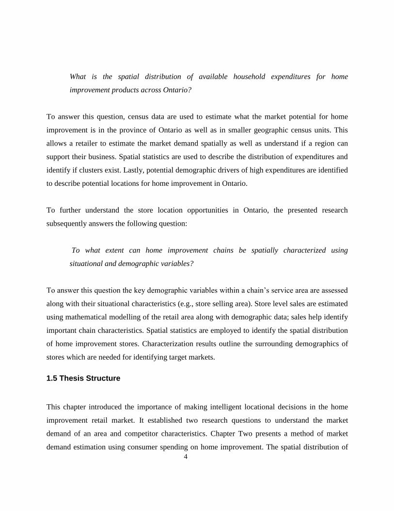
What is the spatial distribution of available household expenditures for home

improvement products across Ontario?

To answer this question, census data are used to estimate what the market potential for home

improvement is in the province of Ontario as well as in smaller geographic census units. This

allows a retailer to estimate the market demand spatially as well as understand if a region can

support their business. Spatial statistics are used to describe the distribution of expenditures and

identify if clusters exist. Lastly, potential demographic drivers of high expenditures are identified

to describe potential locations for home improvement in Ontario.

To further understand the store location opportunities in Ontario, the presented research

subsequently answers the following question:

To what extent can home improvement chains be spatially characterized using

situational and demographic variables?

To answer this question the key demographic variables within a chain’s service area are assessed

along with their situational characteristics (e.g., store selling area). Store level sales are estimated

using mathematical modelling of the retail area along with demographic data; sales help identify

important chain characteristics. Spatial statistics are employed to identify the spatial distribution

of home improvement stores. Characterization results outline the surrounding demographics of

stores which are needed for identifying target markets.

1.5 Thesis Structure

This chapter introduced the importance of making intelligent locational decisions in the home

improvement retail market. It established two research questions to understand the market

demand of an area and competitor characteristics. Chapter Two presents a method of market

demand estimation using consumer spending on home improvement. The spatial distribution of

5

these data is analyzed and the potential demographic drivers of high expenditures are presented.

Home improvement chain store characterization is presented in Chapter Three and spatial

statistics are employed to describe the distribution of stores across Ontario. Key variables in

proximity to a store’s location are identified using regression models. The final Chapter Four

presents conclusions pertinent to the two research questions.

6

Chapter Two: Estimating Market Demand: Expenditures

1.0 Introduction

Retail trade is a highly competitive business sector. Each chain (and to a lesser extent individual

store) must balance supplier and operating costs, appropriate pricing, customer satisfaction and

competition to maintain profitability. With the entrance of big-box chains (having stores range in

size from 20,000 to over 150,000 square feet) in Canada, small format or independent stores are

pressured to maintain profitability in spite of tough competition (Jones & Doucet, 2000). This

competitive intensification can be attributed to the appeal of big-box chains as they offer bulk

purchasing, discount pricing and the advantage of buying multiple products at one location. Big-

box chains, like all retail however, currently face difficult decisions when siting new stores since

many optimal sites have disappeared due to market saturation (Hernandez et al., 1998), and the

ability to attract customers does not directly translate to retail success.

The defining factor for retail success is often attributed to location, location, location (Benoit &

Clarke, 1997; Gonzalez-Benito & Gonzalez-Benito, 2005; Hernández & Bennison, 2000; Jones

& Doucet, 2000; Murray, 2010; Theodoridis & Bennison, 2009). The role of a retail store’s

location is vital since it determines its trade area and the market that it will be able to service and

attract (Gonzalez-Benito & Gonzalez-Benito, 2005). Competitors in close proximity affect

market share acquisition and customer attraction, while same chain stores in close proximity can

cannibalize market share; the location should minimize these effects (Suárez-Vega, Santos-

Peñate, & Dorta-González, 2012). Corporate strategies are determined by the location, and

management tends to view this factor as critical to success (Clarke, Bennison, & Pal, 1997).

Retailers must be aware that they are in essence “marrying” the location for the next few decades

and leaving is very expensive (Hernandez et al., 1998).

Due to the importance of an appropriate location in retail, a number of location assessment

methods have been created over time. Two common methods (which have been around for over

50 years) are checklists and analogues (Clarkson et al., 1996; Hernandez et al., 1998; O’Malley,

7

Patterson, & Evans, 1997; Theodoridis & Bennison, 2009). Using checklists, the retailer

evaluates the site against a set of established criteria, while analogues involves using comparable

stores and sites to assess potential performance (Wood & Reynolds, 2012). These methods rely

on the past experiences of the retailer (Evans, 2011) to identify if a location matches their

criteria. While a simple assessment, like checklists, can give an indication of the quality of a

location, it does not provide an estimation of revenue or market share. Coupling the retailer’s

knowledge (used in checklists or analogues) with the development of new technologies and the

increased availability of market data, newer methods such as Geographic Information Systems

(GIS; Clarke et al., 1997; Murray, 2010), gravity modelling (Benoit & Clarke, 1997) and

Artificial Neural Networks (ANN; Hernández & Bennison, 2000; Reynolds & Wood, 2010;

Wood & Reynolds, 2012) are becoming industry standards for market assessment.

While these advanced location assessment methods can estimate a variety parameters, the

viability of a location for the successful establishment of a retail store begins foremost with

estimating the market demand (Smith & Sanchez, 2003) as it provides the foundation for

subsequent location-based analyses (e.g., sales forecasting; Li and Liu, 2012). Evaluating the

untapped sales potential is important for a market location decision and, in identifying a

literature gap, Mulhern (1997) posits that future research should address topics such as revenue

potential.

The necessity to estimate market demand and recent advances in technology have made possible

the creation of big data for the retail sector, with each chain attempting to learn more about their

customers’ spending patterns via point-of-sale systems, customer databases and, more recently,

chain’s website activity tracking. These data however, being sensitive in nature and key to a

chain’s success at market penetration, are kept private and are hard to acquire. A number of

business analytics companies (e.g., ESRI, Environics Analytics) attempt to model customer

shopping patterns for a variety of sectors, and offer their very expensive data for sale (e.g., Dun

and Bradstreet). In lieu of such data, other businesses, municipalities and researchers must find

cost-effective ways to estimate market demand, typically using available census data.

8

Despite a lack of detail in existing literature describing how to estimate market potential, several

conceptual approaches have been presented. In a study conducted by Ghosh & Craig (1983) to

compare the profitability for two major retail chains, they took a proportion of total potential

revenues of the stores minus the fixed store costs; the potential revenues were modeled by

assuming a fixed expenditure dollar value per family (on a spending category) and multiplying

that by the number of families in an area. To correct for the fact that not all households spend the

same (heterogeneity in economic status), Strother, Strother, & Martin (2009) modeled potential

expenditures by finding the proportion of household income spent on commodities at different

income brackets. These proportions were multiplied by the number of households to estimate the

market demand in an area.

The presented research builds on previous research estimating market potential (e.g., Strother et

al., 2009) by answering three questions. First, as the expenditures are calculated spatially, what

are the spatial patterns exhibited by market demand? Spatial statistics are used to assess and

quantify the spatial distributions of market demand. Second, to what extent can consumer

expenditures match reported store sales? Reported consumer expenditures can be used as a proxy

for market demand, and multiplying the expenditure values by the number of households in a

region yields total spent on a retail sector. Lastly, are there potential demographic variables that

drive consumer expenditures and can these be used as identifiers of market demand?

Demographic variables are regressed against consumer expenditures to identify statistically

significant descriptors of market demand. The following sections will detail the methodology

employed to answer these questions.

2.0 Methods

2.1 Study area

This paper sets out to develop a methodology of estimating market demand for retail trade

spatially. In order to provide a bounded context, the home improvement sub-sector in the

province of Ontario was used as a case study. This is the fifth fastest growing sub-sector in retail

9

trade in terms of revenue and second in terms of number of stores opened; it is one of only two

sub-sectors that have surpassed their number of stores since the 2008 recession (Statistics

Canada. Table 080-0023).

The growing population of the province along with their economic buying power place

significant demand on the home improvement sector. As of 2011, Ontario had a population of

12,851,821 (5.7% increase from 2006) accounting for 38% of the Canadian population; of the

population, 87% live in the 43 Census Metropolitan Areas (CMA) or Census Agglomerations

(CA) where the majority of commercial activity resides (Statistics Canada, 2012). Census family

counts increased by 5.5% from 2006 to 2011 reaching 3,612,205, of which 49.3% had children

24 and under at home (Statistics Canada, 2012). The average forecasted population growth of

Ontario from 2014 to 2017 is expected to be at 1.1% (IHS Global Insight, 2013).

The growing population of the province drives the housing market which accounts for 36.7% of

all national dwellings (4,887,510 Ontario dwellings), of which 55.6% of households lived in

single-detached houses while 16.2% lived in high-rise apartments (Statistics Canada, 2012). As

of 2011, 71.4% of private Ontario dwellings were owned, with 93.4% needing only minor repairs

and maintenance, and having an average 6.4 rooms per dwelling (Statistics Canada, 2013).

Besides existing dwellings, housing starts in Ontario increased by 2.4% from 2008 to 2012, with

60,462 new homes built in 2013 (IHS Global Insight, 2013).

The expanding housing market is supported by the $362.92 billion (2012 at 2007 dollar constant)

real household income in Ontario with a projected 8.3% increase by 2017 (IHS Global Insight,

2013). The investments made by Ontarians in the home improvement market totaled $15.86

billion in sales in 2013 which was an average annual growth of 2.1% from 2008 accounting for

36.8% of all home improvement sales in Canada and almost twice as much as the next highest

grossing province, Quebec (IHS Global Insight, 2013). Home improvement industry sales are

expected to grow 19.1% by 2017, reaching a total sales value of $18.89 billion in Ontario (IHS

Global Insight, 2013).

10

Figure 2.1 - Southern Ontario census subdivisions rendered by the count of home improvement stores

2.2 Data

Data used to model market demand is composed of demographic attributes associated with

geographic census levels, household spending surveys, and existing home improvement store

information. Demographic data for the analysis were acquired from Statistics Canada. These data

are the result of extensive national surveys conducted every five years. As of 2011, the National

Household Survey (NHS)1 replaced the mandatory census, which has placed the quality of the

data into question, due to reduced responses and data suppression (based on the global non-

response rate). To address these concerns, Statistics Canada provides a global non-response

index to identify the accuracy level across different geographic entities. In lieu of the mandatory

1 The NHS User Guide (catalogue no. 99-001-X2011001) details the structure of the survey, the target population,

sampling design, data processing, quality assessment and the dissemination of the data, along with questions asked of the respondents. The entire guide can be accessed from Statistics Canada: http://www12.statcan.gc.ca/nhs-enm/2011/ref/nhs-enm_guide/99-001-x2011001-eng.pdf

http://www12.statcan.gc.ca/nhs-enm/2011/ref/nhs-enm_guide/99-001-x2011001-eng.pdf

11

national census, however, the NHS provides the most suitable publicly available data for a study

at this scale.

NHS data are reported at different census levels (Appendix A) ranging from a provincial scale

(or geography) to census blocks, and are freely available online. The market demand estimation

is performed at three census geographic levels: Census Divisions (CD) – regions/municipalities,

Census Subdivisions (CSD) – cities/towns (Figure 2.1), and Dissemination Areas (DA) –

collection of blocks. For each geographic level, 1431 demographic characteristics are collected

and grouped into 39 sub-topics. These are then grouped into nine major topics covered by the

census and NHS as follows:

Census: 1) Age and Sex, 2) Families, household and marital status, 3) Structural type of

dwelling and collectives, and 4) Language

NHS: 5) Aboriginal Peoples, 6) Immigration and Ethnocultural Diversity, 7) Education

and Labor, 8) Mobility and migration, and 9) Income and Housing

While the NHS provides demographic data for a location, information about spending patterns of

households is collected yearly in the Survey of Household Spending (SHS) and presented

publicly via the Canadian Socio-Economic Information Management System (CANSIM). These

data cover a variety of spending categories at different geographic census units in tabular format.

In addition to demographic and spending data, existing home improvement stores were used in

the spatial analysis of market demand estimation. The North American Industry Classification

System (NAICS) is used to classify business categories in Canada; within the Retail Trade sector

(classified as NAICS code 44-45), the ‘Building material and garden equipment and supplies

dealers’(NAICS subsector code 444) category was chosen for this analysis. The stores classified

as NAICS 444 are considered to be the primary businesses for home improvement retail. Herein,

home improvement is referred to as the process by which one makes renovations or additions to

a dwelling; home improvement stores, then, are assumed to be those which sell materials (e.g.,

12

lumber, paint, grass) and products (e.g., tools) for renovations, additions or maintenance of

homes. While even a small shop selling repair materials is classified as NAICS 444, only 18

major chains (Appendix B; 1,179 stores) were used in this analysis. Of 18 chains, some (e.g.,

Canadian Tire) sell products that can be classified outside of NAICS 444, and are typically sold

at specialty stores (e.g., furniture, sold at The Brick).

The store data (including business name, address, phone number, website and category of

business) were collected from yellow-pages and white-pages directories and geocoded (matched

on a geographic road network). The geocoded stores were then manually verified for positional

accuracy in a GIS using aerial imagery from the Land Information Ontario2 (a branch of the

Ministry of Natural Resources) and street-view imagery available online. The square footage of

each store was calculated by digitizing the visible store footprint at a scale of 1:500 with a

minimum mapping unit of 25 cm.

2.3 Market Demand Estimation Methods

Retail demand can be estimated using consumer expenditures and demographics (Smith &

Sanchez, 2003; Strother et al., 2009). One approach for estimating market demand involves the

summation of known expenditures on specific spending categories for all households in a given

geographic area. An equation to model market demand at any geographic level that contains

counts of households and household income can be stated as follows:

𝐷𝑒𝑚𝑎𝑛𝑑 = 𝑒𝑥𝑝𝑥 ∗ 𝐻𝐻𝑀𝐼 ∗ 𝐻𝐻𝑛

(1)

where 𝑒𝑥𝑝𝑥 is the proportion of average household income spent on home improvement

(𝑥 represents the method – i.e., method one will model 𝑒𝑥𝑝1), 𝐻𝐻𝑀𝐼 represents the median

income of households and 𝐻𝐻𝑛 the count of households. Since household expenditure values are

only reported at the provincial level in Ontario, in order to estimate market demand spatially at

2 Land Information Ontario data warehouse overview - https://www.ontario.ca/environment-and-energy/land-

information-ontario <include date last accessed>

https://www.ontario.ca/environment-and-energy/land-information-ontario

https://www.ontario.ca/environment-and-energy/land-information-ontario

13

lower census levels, the 𝑒𝑥𝑝𝑥 proportion in equation 1 was modeled using four methods to

account for varying spending patterns at different income levels.

While 𝑒𝑥𝑝𝑥 from Equation 1 was modeled by dividing average household expenditure and

average household income, the equation makes use of median household income for the final

estimation of market demand. This is due to the non-normal distribution of household income in

Ontario (Figure 2.2). Since the income distribution is uneven, the median income provides a

better summary statistic for the middle income value as it is not affected by skews and outliers

like the average. Due to Statistics Canada not reporting median household expenditures, the

𝑒𝑥𝑝𝑥 from Equation 1 was modeled using averages, while the equation multiplied this proportion

by the median household income to account for the non-normal distribution, the product being an

average dollar amount spent by each household in the geographic area on home improvement.

Figure 2.2 - Household distribution by income brackets in Ontario, 2011 (Statistics Canada, 2013)

2.3.1 Method One: Basic Spending

The market demand of an area can be calculated using a generic spending category on home

improvement for households in Ontario, similar to Ghosh & Craig (1983). This basic calculation

yields a crude benchmark of potential expenditures in Ontario. The 𝑒𝑥𝑝1 from Equation 1 is

calculated as the ‘Household furnishings and equipment’ general spending category ($2,123;

14

Statistics Canada: Table 203-0021) on home improvement, divided by the Ontario average

household income of $85,772 reported in the NHS (Statistics Canada, 2013).

The result is an estimate of the proportion of household income spent, on average, by each

household in Ontario on home improvement related purchases (2.475%). Substituting 𝑒𝑥𝑝1 =

0.02475 into Equation 1 along with the median household income and household count for

various census levels, provided a basic spending estimate of market demand.

2.3.2 Method Two: Refined Spending Categories

While using a general spending category can create a benchmark for market demand, home

improvement stores (especially large chains as used in this analysis – Appendix B) often sell

products that are part of other spending categories in the SHS. To better represent the spending

categories that coincide with Home Improvement chain stores, Method Two refined the

household expenditure value on home improvement by using 23 spending categories (Table 2.1).

Two spending categories (Luggage per household, and Cutlery, flatware and silverware per

household) that Statistics Canada incorporates in its “Other household equipment” category

(Table 2.1) are not sold in the home improvement stores used for this analysis. Using Environics

Analytics data, it was estimated that these categories represented 4.56% of the subcategory

“Household Equipment” under the “household Furnishings and Equipment” category, which

represented $45.

Aggregating the expenditure category values (Table 2.1) and removing the two spending

categories (i.e., $45), the total average expenditure on home improvement purchases by

households in Ontario is $3057, which is 3.565% of the Ontario average household income (i.e.,

$85,772). Substituting this new value (𝑒𝑥𝑝2 = 0.03565) into Equation 1 yielded an estimate of

expenditures that accounts for spending categories outside of the generic “Household furnishings

and Equipment” category and which are specific to home improvement store sales.

15

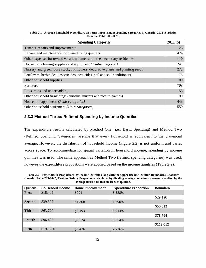
Table 2.1 - Average household expenditure on home improvement spending categories in Ontario, 2011 (Statistics

Canada: Table 203-0021)

Spending Categories 2011 ($)

Tenants' repairs and improvements 26

Repairs and maintenance for owned living quarters 424

Other expenses for owned vacation homes and other secondary residences 110

Household cleaning supplies and equipment (3 sub-categories) 241

Nursery and greenhouse stock, cut flowers, decorative plants and planting seeds 272

Fertilizers, herbicides, insecticides, pesticides, soil and soil conditioners 75

Other household supplies 109

Furniture 708

Rugs, mats and underpadding 55

Other household furnishings (curtains, mirrors and picture frames) 90

Household appliances (7 sub-categories) 443

Other household equipment (4 sub-categories) 550

2.3.3 Method Three: Refined Spending by Income Quintiles

The expenditure results calculated by Method One (i.e., Basic Spending) and Method Two

(Refined Spending Categories) assume that every household is equivalent to the provincial

average. However, the distribution of household income (Figure 2.2) is not uniform and varies

across space. To accommodate for spatial variation in household income, spending by income

quintiles was used. The same approach as Method Two (refined spending categories) was used,

however the expenditure proportions were applied based on the income quintiles (Table 2.2).

Table 2.2 – Expenditure Proportions by Income Quintile along with the Upper Income Quintile Boundaries (Statistics

Canada: Table 203-0022; Custom Order). Proportions calculated by dividing average home improvement spending by the

average household income in each quintile.

Quintile Household Income Home Improvement Expenditure Proportion Boundary

First $18,405 $991 5.388%

$29,130

Second $39,392 $1,808 4.590%

$50,612

Third $63,720 $2,493 3.913%

$78,764

Fourth $96,437 $3,524 3.654%

$118,012

Fifth $197,280 $5,476 2.776%

16

Similar to an ‘if-statement’ used in computer science, the median income from Equation 1 was

compared with the boundaries from Table 2.2, and the Expenditure Proportion for the respective

quintile (Table 2.2) was used for 𝑒𝑥𝑝3. As such, a census unit with a median income between

$29,130 and $50,612 would have 4.590% (𝑒𝑥𝑝3= 0.0459) substituted into Equation 1.

2.3.4 Method Four: Refined Spending by Income Bracket

Similar to the process used for Method Three, the population of households in Ontario was

further broken down by income brackets along with income quintiles. While expenditures are not

reported by income brackets, such an approach yielded expenditure estimates for households in

each bracket. The total expenditure estimate for each census unit was calculated using the count

of households in 13 income brackets (Figure 2.2), the expenditure proportions by income

quintiles (Table 2.2) and by applying Equation 1 with 𝑒𝑥𝑝3 to each income bracket.

When an income bracket falls entirely within a quintile (e.g., $30,000 to $39,999 completely in

Quantile 2), each household in the bracket is assumed to spend using the same expenditure

proportion (the distribution of household income in the bracket is assumed to be normal).

Therefore, applying the entire expenditure proportion to either the lower or upper bracket bound

would result in an average household expenditure value entirely skewed to either the lower or

upper income. Applying the entire expenditure proportion to both bracket bounds would result in

inflating the expenditure value (i.e., each household spends cumulatively at the level of both the

lowest and highest income in the bracket). To estimate the average expenditure value per

households in the bracket, 50% of the expenditure proportion (considered a weight) was applied

to the lower bound and 50% to the upper bound; the two values were summed to yield an

average expenditure value per home in the income bracket. The count of households in the

bracket was multiplied by the average expenditure value to yield the total spending value in the

bracket.

As an example, if the income bracket was $30,000 to $39,999, the expenditure proportion from

Quantile 2 was used (i.e., 4.668%). The lower bracket bound ($30,000) was multiplied by 50%

of the expenditure proportion (i.e., 4.668%) to yield an average expenditure for the lower bound

17

of $669.30. The same approach was taken for the upper bound ($39,999) to yield $892.40;

adding these two values resulted in an average expenditure amount of $1,561.70 for each

household in the income bracket.

An income bracket that crosses an upper income quintile boundary (i.e. $50,000 to $59,999)

would have modified weights to account for the difference in spending proportions (a different

expenditure proportion is applied to each bound). If the income quintile boundary was to fall in

the middle of the income bracket (i.e. $55,000) it would be safe to assume that each bound

should have equal weighing when applying the expenditure proportions. However, if the

boundary was closer to an income bracket bound, the bound’s expenditure proportion was given

less weight (given the assumption of normal household income distribution in the bracket).

To calculate the appropriate weight for the lower income bracket bound, the bracket bound was

subtracted from the income quintile boundary value, and the result divided by the income bracket

range. The quotient was used as the expenditure proportion weight for the lower income bracket

bound. The same approach was taken for the upper income bracket bound, however the income

quintile boundary was subtracted from the upper bound.

Using the $50,000 to $59,999 income bracket as an example, the lower bracket bound was

subtracted from the income quintile boundary ($50,612; Table 2.2) and divided by the bracket

range ($59,999 - $50,000) to yield an expenditure proportion weight of 6%. The upper weight

was reduced by the income quintile boundary and proportioned by the bracket range to yield a

weight of 94%. The lower bracket bound estimated expenditure was calculated using the 4.590%

proportion (Table 2.2) and the 6% weight, and the upper bracket bound estimated using the

3.913% proportion (Table 2.2) and the 94% weight. The summation of these two values

produced an average expenditure per household of $2,344.57, in the $50,000 to $59,999 income

bracket. The expenditures amounts for each bracket are shown in Table 2.3.

18

Table 2.3 - Expenditure Dollar Values by Household Income Bracket

The implementation of the final calculation is performed in a GIS by multiplying the expenditure

dollar value for each income bracket by the count of households in that bracket, and aggregating

the products. This method no longer focuses on the median income of the census unit but the

distribution of income and ensures the appropriate expenditure is assigned to each bracket.

2.4 Assessment of Expenditure Estimation Methods

The four methods presented were used to estimate total expenditures on home improvement

products using 2011 census data. Since these expenditures represent actual spending in 2011,

provincial sales in the retail sectors servicing these spending categories can be used to evaluate

the expenditure estimation methods. While home improvement stores (especially big-box

retailers) sell products that can be outside of their NAICS category, or spending on home

improvement categories can take place in stores not in NAICS 444, a detailed accuracy

assessment of the presented methods cannot be provided. It is thus understood that this

comparison is to provide an estimate of the performance of these methods and will not produce

exact error quantifications.

Statistics Canada reports retail trade sales by NAICS sectors. Aggregate monthly sales for the

year of 2011 are reported for all the stores classified as NAICS 444. Based on Statistics Canada’s

quality indicator for these values, the sales for the NAICS 444 stores are rated as “Very Good”.

These monthly sales are aggregated to produce the total sales in the NAICS 444 subsector in

Quintile Income

Boundary

Low Income

Bracket

High Income

Bracket

Lower

Weight

Upper

Weight

Low Bracket

Proportion

High Bracket

Proportion

Low Expend

Value

High Expend

Value

TOTAL

Expenditure

4,999.99$ 1.00 5.388% 5.388% -$ 269.40$ 269.40$

5,000.00$ 9,999.99$ 0.50 0.50 5.388% 5.388% 134.70$ 269.40$ 404.10$

10,000.00$ 14,999.99$ 0.50 0.50 5.388% 5.388% 269.40$ 404.10$ 673.50$

15,000.00$ 19,999.99$ 0.50 0.50 5.388% 5.388% 404.10$ 538.80$ 942.90$

29,130.00$ 20,000.00$ 29,999.99$ 0.91 0.09 5.388% 4.590% 983.85$ 119.80$ 1,103.65$

30,000.00$ 39,999.99$ 0.50 0.50 4.590% 4.590% 688.50$ 918.00$ 1,606.50$

40,000.00$ 49,999.99$ 0.50 0.50 4.590% 4.590% 918.00$ 1,147.50$ 2,065.50$

50,612.00$ 50,000.00$ 59,999.99$ 0.06 0.94 4.590% 3.913% 140.45$ 2,204.11$ 2,344.57$

78,764.00$ 60,000.00$ 79,999.99$ 0.94 0.06 3.913% 3.654% 2,202.71$ 180.65$ 2,383.36$

80,000.00$ 99,999.99$ 0.50 0.50 3.654% 3.654% 1,461.60$ 1,827.00$ 3,288.60$

118,021.00$ 100,000.00$ 124,999.99$ 0.72 0.28 3.654% 2.776% 2,633.95$ 968.68$ 3,602.63$

125,000.00$ 149,999.99$ 0.50 0.50 2.776% 2.776% 1,735.00$ 2,082.00$ 3,817.00$

150,000.00$ 1.00 2.776% 2.776% 4,164.00$ -$ 4,164.00$

19

2011 (January to December) of $9.614 billion (Statistics Canada. Table 080-0020). This value is

compared to the aggregate expenditure estimation from each of the four methods presented,

applied to three geographic census units of increasing spatial specificity (CD, CSD and DA

levels). While some of the stores can sell outside of their NAICS classification (e.g., furniture

sales), it is assumed that the NAICS 444 sales are coming from the home improvement stores.

The second expenditure method uses more spending categories for the estimation to match what

a big-box home improvement store would sell. The results at the DA level are compared to

proprietary data provided by Environics Analytics (EA), who enhance the reported Statistics

Canada data by conducting additional survey and modelling research. The EA data are reported

at the DA level and therefore can be compared one-to-one against the four method estimates.

Correlation is used to test the similarity between the EA data and the different estimation

methods at the DA level.

2.5 Spatial Analysis

To evaluate the spatial distribution of expenditures and discover if there are patterns or clusters

in the data, spatial statistics were used. The spatial analysis was performed at the DA (19,964

census units) level only as the resolution of the data is finer and neighborhood variation is more

evident than at the CSD (574 census units) or CD (49 census units) levels. Summary statistics

were also presented for urban and non-urban expenditures.

Firstly, the Global Moran’s I calculation of spatial autocorrelation was used to find if there were

clusters among the expenditure results. This calculation was also used incrementally (increasing

the search distance) to find the distance that yields the most extreme autocorrelation (a necessary

parameter for hot spot analysis). Secondly, Getis-Ord hot spot analysis was performed to identify

where clusters of high expenditures (or hot spots) are. The analysis was performed at a 95%

confidence level, therefore only hot-spots with a z-score over 1.65 and a p-value of less than 0.05

were assessed for clustering. Lastly, Anselin Local Moran’s I was applied to check where high

20

and low clusters occurred as well as to identify where outliers were located (areas of high

expenditures where low are expected).

These cluster analyses were overlaid with CMA/CA areas to find if high expenditures were

particular to urban areas or if they could also be expected in rural areas. The proximity of home

improvement stores to these clusters (as well as counts by clusters) were computed to assess

whether the home improvement subsector is located near areas of high-expenditure. Total and

average square footage of stores in expenditure hot spots was compared to areas outside such

clusters, to identify areas of high market demand translate to large store footprints.

2.5.1 Potential Drivers of Expenditure

To identify if potential drivers of home improvement expenditures exist, stepwise regression3

was used to check the statistical significance of demographic variables in explaining

expenditures. From the 1,431 demographic variables collected in the quinquennial Canadian

census and NHS, 930 (65%) variables detail subdivisions of languages spoken, ethnic origin and

places of birth. A further 196 variables are subdivisions of general population descriptors (e.g.,

from couples with children, lone male parent with children, lone female parent with children),

leaving 305 general population variables. To align with literature on demographic topics

identified as important to retail (Table 2.4), a deductive selection of variables relevant to home

improvement from each topic was performed.

Table 2.4 – Demographic topics covered in literature as important to home improvement retail.

Demographic Topic

(Girard et al., 2003)

(Rhee & Bell, 2002)

(Gijsbrechts, Campo, & Goossens, 2003)

(Fox, Montgomery, & Lodish, 2004)

(Baltas & Papastathopoulou, 2003)

(Smith & Sanchez, 2003)

Age ✔ ✔ ✔ ✔

Education Level ✔ ✔ ✔ ✔ ✔

Income ✔ ✔ ✔ ✔ ✔ ✔

Ethnicity ✔ ✔

Employment ✔ ✔

Family characteristics

✔ ✔ ✔ ✔

3 Environmental Systems Research Institute’s (ESRI) ArcGIS platform: Exploratory Regression Tool

21

Labor ✔ ✔ ✔ Dwelling Characteristics

✔ ✔

The chosen variables were absolute counts (e.g., private dwellings), averages/medians (e.g.,

median commuting duration) and counts of variable subdivisions (e.g., count of households

owned from all households). In the case of variable subdivisions, the largest proportions of the

parent categories were selected. Similarly, where detailed subdivisions were provided for a

demographic topic (e.g., age breakdown), the subdivisions were aggregated into the most

relevant group for home improvement (e.g., population aged 25 to 64, assumed to be the working

population). From the 305 general population variables, 26 were selected for the stepwise

regression (Table 2.5). The private dwellings count (variable 1) and median household income

(variable 26) were excluded from the stepwise regression as expenditures were calculated using

these two variables. Their usage in a regression model to explain expenditures would result in a

circular relationship.

Table 2.5 – Selected demographic variables for stepwise regression. Percentages in brackets represent the proportion of

the total variable population. Numbers in brackets represent proportion of parent variable population (e.g., for dwelling

type, the parent variable population is all dwellings).

1 Private Dwellings count 14 Dwelling Status: Minor or reg. repair (93%)

2 Population aged 25 to 64 years (55%) 15 Dwelling Status: Major repair (7%)

3 Median age of population 16 Average number of rooms per dwelling

4 Population married/common-law (couple) (58%) 17 Household: Owned (71%)

5 Dwelling type: Detached (single and semi) (61%) 18 Household: Rented (28%)

6 Dwelling type: Apartment (30%) 19 Household maintainers: 1 (58%)

7 Dwelling type: Row (8%) 20 Household maintainers: 2 (39%)

8 Average number of persons in household 21 Spending less 30% of income on HH (73%)

9 Immigrants (29%) 22 Average monthly costs (owned shelter)

10 Mobility: Non-movers (previous year) (88%) 23 Average value of dwelling

11 Education: High School and over (81%) 24 Household income: 0 - $100,000 (71%)

12 Labour: Employment rate 25 Household income: over $100,000 (29%)

13 Median commuting duration 26 Median household income

The stepwise regression was performed on DAs classified as hot spots (clusters of high

expenditures), cold spots (clusters of low expenditures) and random census units (DAs that did

not exhibit statistical clustering), to identify if there were potential demographic variables

influencing high expenditures.

22

3.0 Results

The first step in assessing the spatial patterns of expenditures as set posited in the first research

question is to visualize the results at the three census levels. While four estimation methods are

put forward for expenditure estimation, method four (using the most granular data) is used for

visualization. Similarly, only southern Ontario is visualized as the northern region hosts only

5.7% of the provincial population, produces 5.7% of the provincial expenditures, and exhibits

very little to no visible spatial patterns in expenditures.

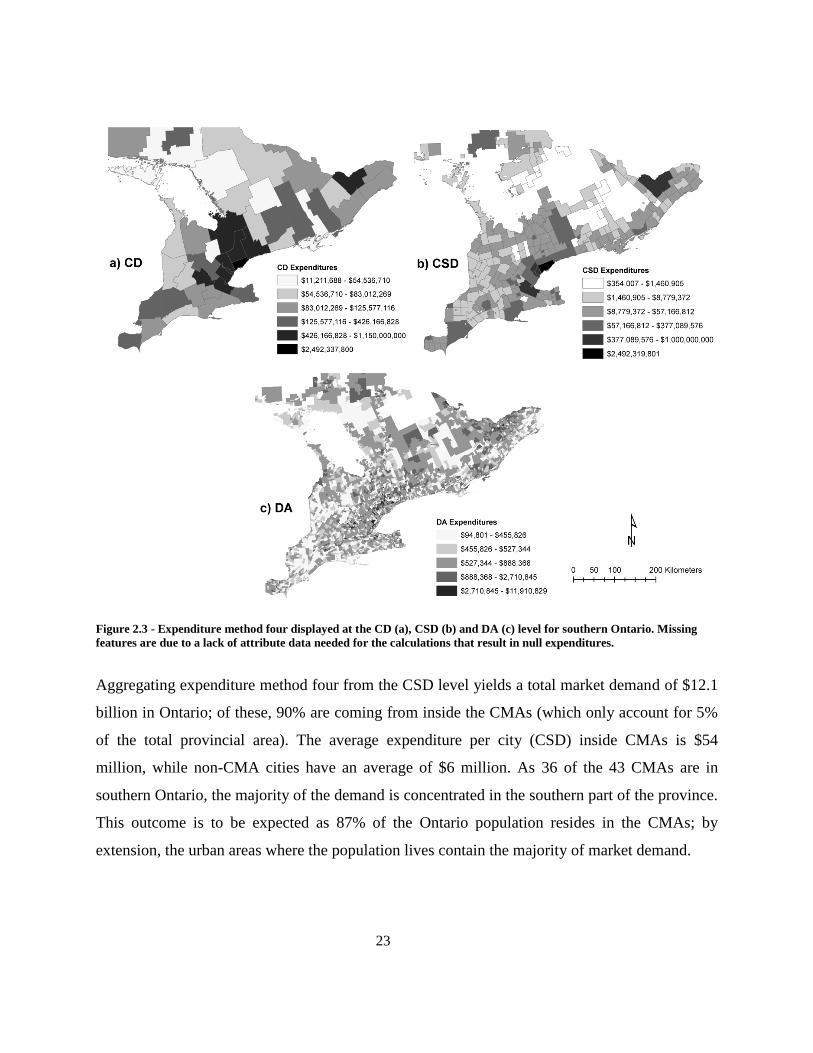
At the CD level (Figure 2.3a), visualizing method four does not reveal any strong patterns,

except that the Greater Toronto Area (GTA)4 yields the highest expenditure values in Ontario

(43% of provincial total). Other large urban centers such as Ottawa (9% of expenditures),

Waterloo (4%), and Hamilton (4%) also show higher levels than the rest of the province.

Similarly, method four at the CSD level (Figure 2.3b) shows patterns of high expenditure in the

GTA and less accentuated patterns in the other urban areas. However, part of central Ontario is

missing due to lack of data (missing demographic data). Out of the 574 CSD, 250 have no data

and as such, yield no results for the expenditure calculations. The largest expenditure value

($2.49 billion) is attributed to the City of Toronto, with the next four highest being Ottawa ($970

million), Mississauga ($633 million), Hamilton ($490 million), and Brampton ($409 million).

Visualizing method four at the DA level (Figure 2.3c) does not reveal any obvious patterns.

Rather, areas of high expenditure are scattered throughout southern Ontario, however no

particular clustering is visible. This geographic level is less useful for visualization as it is for a

more detailed analysis such as statistical clustering, and for identifying neighborhood patterns.

4 A local name associated with the Toronto CMA which has 24 CSDs associated with it, including (by population

rank): Toronto, Mississauga, Brampton, Markham, and Vaughan.

23

Figure 2.3 - Expenditure method four displayed at the CD (a), CSD (b) and DA (c) level for southern Ontario. Missing

features are due to a lack of attribute data needed for the calculations that result in null expenditures.

Aggregating expenditure method four from the CSD level yields a total market demand of $12.1

billion in Ontario; of these, 90% are coming from inside the CMAs (which only account for 5%

of the total provincial area). The average expenditure per city (CSD) inside CMAs is $54

million, while non-CMA cities have an average of $6 million. As 36 of the 43 CMAs are in

southern Ontario, the majority of the demand is concentrated in the southern part of the province.

This outcome is to be expected as 87% of the Ontario population resides in the CMAs; by

extension, the urban areas where the population lives contain the majority of market demand.

24

3.1 Comparison of Estimation Methods

Addressing the second research question, the Ontario expenditure estimations are compared to

home improvement sales to estimate the performance of the four methods. Aggregating the 2011

monthly sales for the NAICS 444 sub-sector yields a total of $9.614 billion (Statistics Canada:

Table 080-0020). This value represents spending by Ontarians on home improvement directly, or

more specifically the “Household furnishings and equipment” general spending category. Since

methods two, three and four use more spending categories than the generic “Household

furnishings and equipment” (to match what a big-box store would be selling) it is acknowledged

that these methods will significantly differ from the $9.614 billion baseline. As such, in order to

test the method performance, method one, three and four using only the “Household furnishings

and equipment” spending category, are compared to the NAICS 444 sales (Figure 2.4).

Figure 2.4 - Comparison of aggregated expenditure estimations from Method One, Three and Four using only the general

spending category "Household furnishings and equipment” to NAICS 444 sales of $9.614 billion in Ontario for 2011

Increasing demographic data granularity from method one to three and then to four brings the

aggregate results closer to the $9.614 billion sales. Effectively, each subsequent method makes

use of finer resolution data and improves the representation of heterogeneity in household

income. Similarly, as the spatial units change from the coarse CD level (49 census units in

25

Ontario), to CSD (574 units) and then DA (19,964 units), the estimates come closer to matching

provincial aggregate sales. Method Three at the DA level estimated sales best with an

underestimation of $7.7 million (error of -0.08%). Method four at the CSD and DA level,

however, performs poorly; comparing the results to the pattern shown at the CD level, it is

expected that method four would perform better than method one and three at the CSD and DA

level.

To identify if data suppression caused the reduced accuracy in method four, the census

demographic household counts by income bracket were verified against the NHS household

counts for each census geography (Table 2.6). The values reported at the CD, CSD and DA

levels are for smaller census units (finer data); however, the aggregate of all units at a level has

to match the total number of dwellings in Ontario as reported in the NHS for the province. A ±10

discrepancy is allowable between census units; this value accounts for rounding as the

geographic level becomes smaller.

Table 2.6 - Dwelling counts by income bracket reported by the NHS for Ontario and compared to the aggregate dwelling

counts at the CD, CSD and DA levels for 2011

Comparing the CDs to the NHS, one-to-one match (excluding the ±10 allowable discrepancy at

each bracket) is observed. This validates that the CDs are not affected by data suppression or by

missing data; ideally, the expenditure results from these geographies should be very accurate.

Category NHS CD CSD DA

Under $5,000 123,775 123,775 120,500 46,315

$5,000 to $9,999 78,005 77,985 75,760 22,385

$10,000 to $14,999 143,390 143,405 139,870 64,475

$15,000 to $19,999 211,140 211,165 206,060 117,440

$20,000 to $29,999 405,725 405,725 396,175 300,430

$30,000 to $39,999 425,410 425,410 415,080 321,135

$40,000 to $49,999 425,720 425,725 416,120 320,715

$50,000 to $59,999 398,705 398,700 390,800 291,220

$60,000 to $79,999 680,850 680,855 666,970 622,590

$80,000 to $99,999 552,660 552,670 542,655 477,405

$100,000 to $124,999 497,970 497,965 490,335 416,570

$125,000 to $149,999 331,460 331,480 326,740 231,965

$150,000 and over 611,840 611,845 605,580 545,070

Total Dwelling Counts 4,886,650 4,886,705 4,792,645 3,777,715

26

The CSDs suffer losses in household counts compared to the NHS of 2,200 to 13,880 per

bracket, which corroborates missing data in the expenditures map (Figure 2.3). These values are

affected by lack of data (or data suppression) which in turn yields aggregate expenditure results

less than the CD estimates (Figure 2.4). Lastly, the DAs are missing substantial counts especially

in the lower income brackets. In turn, this creates a total dwelling count which is 1,108,935 less

than the NHS. This explains the drop in accuracy of method four at the DA level (the geography

which is performing best in the other two methods), as method four heavily relies on the counts

by income brackets.

While the comparison of the general home improvement category with the NAICS 444 sales for

method one, three and four is an appropriate assessment of the performance of the three methods,

in order to test the quality of the data of the refined spending categories, the results are compared

against the industry standard data provided by EA. The EA data provide spending values for the

same categories that Statistics Canada reports (Table 2.1) along with other finer sub-categories at

the DA level. As these data are reported for 2013 and the census data are for 2011, a direct error

quantification cannot be performed; however, a correlative comparison is performed on methods

two, three and four using the refined census categories and matching EA categories (Table 2.7).

Table 2.7 - Comparison of aggregated expenditures for Ontario from the EA dataset (year 2013) and methods two, three

and four using the refined spending categories (year 2011). Pearson’s R correlation is used to compare the expenditure

values from the EA data to the analysis data for each DA (19,964 values).

Despite the time difference of the data and the suppression effect on the DAs (for method four),

the correlative comparison reveals that the analysis results are very similar to the EA data. As the

granularity is increased from methods two through four, the Pearson’s R coefficient increases

from 0.85 to 0.87, showing an increase in comparability between the values. To reconcile the

date difference between the EA and census data, the inflation rate from 2011 to 2013 for the

Year Aggregate Expenditures Correlation

Environics Analytics 2013 15,297,857,699.00$ -

Method Two 2011 12,389,619,739.54$ 0.85

Method Three 2011 13,082,114,444.87$ 0.87

Method Four 2011 10,078,056,232.40$ 0.87

27

“Household operations, furnishings and equipment” category (assumed to be representative of

the home improvement categories) is calculated (3.128%; Statistics Canada: Table 326-0021)

and multiplied by the census expenditures. The absolute difference between the EA data and the

census expenditures is calculated, and extreme differences (larger than 1.5 standard deviations)

are assessed. Out of the 1,057 DAs that have extreme differences, 864 (82%) are within the

Ontario CMAs and 499 (47%) are within the Toronto CMA.

There are two reasons for these extreme differences. First, there is a change in dwelling counts

from 2011 to 2013 (i.e., new dwellings built). As a result, DAs with a large difference in

dwelling counts will also have a large difference in expenditures. Second, EA’s use of

psychodemographic data allows for the estimation of spending based on other factors than just

household income; therefore, each DA’s expenditure is calculated based on a segmentation class

rather than an average expenditure value as used in this paper.

3.2 Spatial Analysis of Dissemination Area level Expenditures

The visual representation of expenditures at the CD and CSD level provides a high-level

overview of spatial economic suitability for the home improvement market in Ontario. The two

levels identify a large geographic area (i.e. region or city) as economically suitable for store

location however it does not present neighborhood or locally suitable clusters (such as a DA or

group of DAs). Moreover, it is important to identify spatial clusters rather than individual DAs,

as neighborhoods (or groups of DAs) have more cumulative spending power.

Performing a Global Moran’s I spatial autocorrelation assessment on the DAs using expenditure

method three (best performing out of the four, at the DA level) results in a Moran’s I index of

0.097 with a z-score of 34.79 and p-value of 0.000, which means that there is less than a 1%

chance that this distribution is due to . Therefore, there are statistically significant clusters of

expenditures at the DA level. This finding contributes to answering the first research question

pertaining to the spatial distribution of market demand, showing that there are statistically

significant clusters.

28

The results of the incremental Global Moran’s I analysis show two critical distances (distances at

which clusters exhibit most extreme spatial autocorrelation) occurring at 2,400 meters and 5,500

meters. As the average search distance that ensures each DA is adjacent to eight neighbors (an

important optimization for cluster analysis) is 4,013 m, the 5,500 m distance band was used. The

same approach was applied again with smaller increments on the 5,500 m band resulting in a

statistically significant search distance of 5,430 m.

To identify spatially where these clusters are occurring however, the results from the Getis Ord

hot spot and Anselin’s cluster analyses are evaluated. Performing a Getis Ord Hot Spot analysis

on the method three expenditure results at the DA level using a search distance of 5,430 m for

neighbors, identifies DAs as belonging to: hot spots – neighboring DAs with high expenditure

potential (4,555 DAs), cold spots – neighboring DAs with lower expenditure potential (4,688

DAs) and random (9,923 DAs) (Figure 2.5). All the hot spot clusters are contained within the

CMAs, with the exception of two locations: Saugeen Shores Township and Wilmot Township.

Similarly, the cold spots are contained by the CMAs with the exception of a cluster in the

Greater Napanee Township.

The top five CMAs that have the highest proportion by area of hot spot clusters are: Toronto

(27.74%), Kitchener (25.69%), Ottawa (21.22%), Oshawa (19.78%), and Hamilton (16.22%)

(Table 2.8). Comparing the median incomes in the hot spot clusters with those of the CMAs that

they fall within, the hot spot medians are on average $32,820 higher. Ordering these top five

CMAs by the proportion of CMA expenditures they contain relative to total expenditure in the

CMA shows Toronto (56.45%) first, followed by Ottawa (46.31%), Hamilton (23.37%), Oshawa

(17.96%), and Kitchener (13.13%). While these hot spot clusters have the highest market

demand within the CMAs, the remaining neighborhoods in the CMAs also have a positive

market demand, cumulatively making these CMAs (Table 2.8) prime locations for home

improvement from an economic standpoint.

29

Figure 2.5 - Getis Ord hot spot analysis on expenditure Method Three at the DA level results overlaid with CMAs in

Sothern Ontario. Statistically significant hot spots have z-scores > 1.65 and p-values < 0.05, while statistically significant

cold spots have z-scores < -1.65 and p-values < 0.05, to ensure a 95% confidence level.

Table 2.8 – Comparison of CMA statistics to in-CMA hot spot statistics. ‘CMA expend’ represents the total buying power

of the CMA, ‘Hot Spot Area (%)’ is the proportion of the CMA area the hot spot covers, ‘Hot Spot Expend’ is the

aggregate buying power in the cluster and ‘Hot Spot Expend (%)’ is the proportion of CMA expenditures contained in

the cluster.

CMATotal Area

(km2)

Median

IncomeCMA Expend

Total Area

(km2)

Hot Spot

Area (%)

Median

IncomeHot Spot Expend

Hot Spot

Expend (%)

Toronto 6,280.64 70,365$ 5,585,948,453.36$ 1,742.17 27.74% 89,040$ 3,153,058,988.78$ 56.45%

Kitchener 843.04 68,906$ 494,242,411.04$ 216.55 25.69% 97,171$ 64,898,318.68$ 13.13%

Ottawa 3,395.10 76,066$ 1,095,885,128.61$ 720.30 21.22% 102,192$ 507,551,894.21$ 46.31%

Oshawa 909.26 76,816$ 377,223,022.84$ 179.85 19.78% 105,344$ 67,738,833.65$ 17.96%

Hamilton 1,409.85 65,851$ 753,818,051.27$ 228.73 16.22% 101,084$ 176,129,945.40$ 23.37%

Guelph 605.75 71,597$ 152,076,866.27$ 65.63 10.84% 93,645$ 15,073,546.47$ 9.91%

London 2,694.20 58,405$ 480,505,850.36$ 91.30 3.39% 106,995$ 45,180,743.22$ 9.40%

Kingston 2,143.07 63,564$ 169,629,678.97$ 36.15 1.69% 104,439$ 14,222,023.92$ 8.38%

Windsor 1,040.25 57,942$ 309,262,153.46$ 17.45 1.68% 105,076$ 18,759,135.73$ 6.07%

Hot Spot StatisticsCMA Statistics

30

In order to further understand the variation of expenditure within the hot or cold spot clusters,

Anselin Local Moran’s I results at the DA level are evaluated. The results of the Local Moran’s I

analysis are very similar to that of the Getis Ord. The hot spot clusters from Getis Ord contain

High-High (HH) clusters (statistically significant, at a 95% confidence level, groups of high

expenditure DAs) and Low-High (LH) outliers (a lower expenditure DA surrounded by high

expenditure DAs). The cold spot clusters from Getis Ord contain Low-Low (LL) clusters and

High-Low (HL) outliers. Like the Getis Ord analysis, the Anselin clusters are limited to the

CMAs with the exception of two HH cluster groups located (similarly to the Getis Ord) in

Saugeen Shores Township and Wilmot Township.

Table 2.9 - DA level statistics by Anselin Local Moran’s I cluster and outlier analysis. The ‘Random’ label represents ‘Not

Significant’ clusters from Anselin’s analysis (DAs with random expenditure distributions)

The HH clusters have a higher median income and mean dwelling count by DA than the random

(or not significant) DAs, producing 16% of the total Ontario expenditures (Table 2.9). The

Anselin HH clusters are more refined than the larger Getis Ord hot spots narrowing the location

selection by economic suitability. In contrast, the LL clusters, have lower median incomes and

mean dwelling counts by DA than the random DAs producing only 2.0% of the total

expenditures. The HL outliers (present in 27 of the 35 cold spots) have higher mean dwelling

counts than the HH clusters and although the median income is lower than both the HH cluster

and random DAs, the mean expenditure per DA is $1.77 million (just slightly lower than the HH

clusters), overall producing 3.4% of the total expenditure with just 1.3% of the DAs. This has

important implications for businesses located in cold spots, since the HL outliers that are

scattered throughout the cold spots are valuable segments for the home improvement market in

such areas.

Cluster Type DA Count Mean Dwellings Median Income Mean Expend Total Expend

High-High 1151 605 91,954$ 1,846,313$ 2,125,106,692$

Low-High 542 158 64,644$ 369,911$ 200,491,866$

Low-Low 841 185 40,359$ 325,622$ 273,848,011$

High-Low 250 731 60,282$ 1,767,608$ 441,901,953$

Random 16465 227 71,797$ 609,825$ 10,040,765,923$

31

Lastly, comparing where existing home improvement stores have located and their average

square footage in these high or low expenditure clusters can validate if these expenditures are

important. Of the 1,179 home improvement stores in Ontario (Appendix B), 788 (66.8%) are

within the CMAs. While the performance of the stores (sales) is not reported, the average

footprint area in expenditure clusters is compared to average areas outside clusters. Of the 875

locations of the dominant home improvement chains (i.e., Lowe’s, Home Depot, Canadian Tire,

Home Hardware, and Rona), 37% are within five kilometers of a hot spot cluster while the

average footprint area for the 410 (all) stores within the five kilometers buffer is 53,582 square

feet (Table 2.10). The total floor space (square footage) of the 410 stores within the five

kilometers of expenditure hot spot clusters, is just 64,139 square feet less that the total floor

space of all the stores located in random DAs (no significant clustering). It is evident that the

higher the market demand, the more stores in close proximity to high expenditure clusters and

the larger these stores are, as they are able to be supported by the surrounding market.

Table 2.10 – Area statistics of home Improvement stores and store counts by CMA, Getis Ord, and Anselin clustering.

Store Type (Big-Box, Small Chain, and Major Competitor) are defined in Appendix B.

Type Store Count Mean Total

Big

Box

Small

Chain

Major

Competitor

In CMA 788 43,864 34,565,202 666 122 600

Outside CMA 391 15,417 6,027,957 312 79 275

Random 817 27,645 22,032,699 653 144 579

Hot Spot 149 52,546 7,829,340 131 18 121

Hot Spot 2 km 281 52,682 14,803,561 244 37 226

Hot Spot 5 km 410 53,582 21,968,560 350 60 325

Cold Spot 213 43,546 9,275,212 175 38 158

HH 79 61,913 4,891,147 72 7 66

LH 8 34,720 277,763 5 3 5

LL 32 25,486 815,567 22 10 20

HL 30 64,576 1,937,291 24 6 21

Store Count By TypeFootprint Area (Sq Ft)

Getis Ord

Hot Spot

Analysis

Anselin

Local

Moran's

I

32

3.3 Potential Drivers of Market Demand

The stepwise regression identified a number of demographic variables that influence

expenditures in hot spot and cold spot clusters, as well as random DAs. The identified variables

were used as predictors of expenditure estimates in a linear regression model (Table 2.11) to

answer the final research question on potential drivers of market demand. Two variables that

have a significant influence on expenditures in hot spot clusters (more so than for random DAs)

are counts of households with income over $100,000 and count of dwellings owned. The

combination of the four variables used in the regression for hot spot clusters (Table 2.11)

describes 91% of the variation in expenditures.

Comparing the coefficients of dwellings owned and the high earning households to those of the

same variables in the models for cold spot clusters and random DAs, shows that these two

variables have a significant impact on household expenditures and are potential drivers of market

demand. Regions with a larger number of owned dwellings that are characterized as high-

earning households are important for the home improvement retail market in Ontario.

Table 2.11 - Linear regression model results (DA level) for statistically significant predictors of expenditures in hot spot

and cold spot clusters, as well as random DAs. All coefficients are significant at the 99% level.

Variable Hot Spot Cold Spot Random

Employment Rate 1386.91

Dwellings: Owned 1630.25 333.84

Two household maintainers 1485.00 1218.07

Spending less than 30% of household income on shelter costs 1846.46 2054.25

Average monthly shelter costs for owned dwellings -151.14

Average value of dwelling 0.09

Household with income over $100,000 4063.03 1647.95 2167.90

Observations 4555 4688 9923

Adjusted R2 0.91 0.89 0.92

33

4.0 Discussion

As the number of home improvement retail businesses increase in Ontario and the prime

locations become occupied (e.g., Toronto has 19% of the Ontario home improvement stores),

retailers need methods of market estimation to understand the spatial distribution of potential

expenditures. While big-box chains have the capacity to acquire expensive market analyses from

consultants and retail analyst, the analysis presented in this paper has demonstrated several

methodologies for market assessment using publicly available data that match sales data and

compare well against proprietary data provided by Environics Analytics, which some would

argue is the industry standard for business analysis in Canada. Statistics Canada’s SHS

categories can be used to estimate total dollars spent on home improvement in Ontario and other

provinces in Canada. These values can also be used as a proxy of home improvement market

demand.

The estimation of market demand is performed using four different methods for two reasons.

First, such an approach simulates different scenarios of varying data availability. In their

modeling of market demand, Strother et al. (2009) had access to spending by income brackets;

this was important to match the appropriate spending value with the economic power of the

study area. While this breakdown is not provided in the SHS, a method incorporates spending by

income quintiles (finer resolution data) to provide a better estimation. The second reason pertains

to the geographic level these data are reported at. The SHS only reports spending at the

provincial level, and since this study estimates buying potential spatially at finer geographic

levels (i.e. CSD or DA) different methods increase in complexity to adjust the spending value

appropriately to the local study area’s economic potential (i.e. the median income of one CSD or

one DA).

Using the generic home improvement spending category from the SHS, a baseline of market

demand can be estimated for every census unit in Ontario. However, this number treats each unit

34

as representative of provincial average spending and does not take into account other categories

that home improvement retailers are selling. To adjust for this, using different categories that

pertain to home improvement retail can provide a better representation of spending at such

stores, despite still treating each census unit as representative of the provincial average spending.

Such an approach along with the availability of data however, facilitates the possibility of

estimating market demand for any retail sector. Spending by income quintiles is used to

approximate spending at different economic levels, and to match each census unit’s median

income with an appropriate proportion of spending on home improvement. Lastly, while

spending at lower census units is not reported, building on the last approach, spending can be

estimated for each income bracket to adjust for the heterogeneity of household income within the

census unit.

While the home improvement sub-sector of retail trade has been used as a case study for this

market demand estimation methodological development, the approach described in this paper

can be used to estimate market potential for any retail sector. As data availability can vary for

different regions, the most suitable method can be used to create expenditure estimations. These

methods along with publicly available data can provide an overview of the market demand for a

retailer’s chosen area and coupling these results with other market data and assessment methods

(i.e. gravity modeling and competitive evaluation) can indicate what resources are left for the

incoming business.

The methodology for market demand estimation can be applied not only for other retail sectors,

but for other provinces and countries where similar data are available. The different methods

presented make use of different datasets and granularity of data to simulate data availability or

lack thereof. While some governments will report very granular retail and spending statistics,

some will present very coarse data. The assessment of the four expenditure estimation methods

both against provincially reported sales and industry data provide insight into the level of

accuracy that can be expected when employing one of the methods with varying levels of data

availability.

35

Although such a methodology is important to retailers, municipalities can also benefit from such

an assessment. As a municipality attempts to attract business using various incentives,

understanding if their region has the market demand (in light of existing competition) for such a

business is a key piece in their proposal. The methodology for market estimation presented in

this paper allows municipalities to produce an accurate representation of the spending capacity in

their region, especially as local government benefit from their own internal economic data.

Moreover, planning departments need to better allocate zoning policies in light of development

pressures from large retailers. Using market demand estimation methods along with demographic

forecasts, planners can anticipate increases in market demand and the necessity of zoning for

retail or other commercial land uses.

4.1 Beyond Expenditures

Estimating market demand on its own can show where the expenditure potential is located along

with the spatial patterns and demographic drivers; however, it does not reveal how much of the

capacity is used. While the total market potential is important for a retailer (i.e. if the total

potential is below some critical threshold, the location is dropped altogether), understanding how

much is left in light of competition is very important (Prendergast, Marr, & Jarratt, 1998; Roig-

Tierno, Baviera-Puig, Buitrago-Vera, & Mas-Verdu, 2013). The remainder can be estimated by

comparing market potential, using the methods presented in this paper, with the actual store sales

of the surrounding competition resulting in a map of surplus and leakage (Strother et al., 2009).

When a region has more demand than it has sales from existing stores it results in leaking

expenditures, meaning that the remaining expenditures not accounted for in the sales must be

spent elsewhere than the region. Economic leakage can signal the absence of key retailers to

absorb the remaining expenditures. Leakage also establishes what demand is not absorbed by the

market, and while each store aims to maximize market share, this leaking amount is already

available despite existing competition. Once identified, such a location would be a very good

candidate for a retailer from an economic standpoint.

36

However, if the region produces more sales than the local market has demand, it is said to be in

surplus. Such an area must be drawing in spending from outside the region and can be classified

as a vital commercial hub. Such an effect could be due to the availability of products and

services not found in the close vicinity of such an area, that make customers gravitate towards

the region. Since surplus can be quantified using the sales to expenditures comparison, a retailer

can assess if the excess expenditure amount can sustain their business alone, outside of future

market share acquisition from their competitors. Similar to areas of high leakage, surplus

identifies areas that have been saturated yet and that can still support other retailers.

Such useful analyses for quantifying existing dollars amiable for retail while taking competition

into consideration begin with a proper estimation of market demand. While sales data are usually

reported for various businesses at varying levels of census geography, market demand values are

seldom available. The methodology proposed in this paper can bridge the gap and create such

data for market assessment.

4.2 Market Demand: Key Piece in Retail Modelling

As previously stated, the presented market demand estimation methods (on their own) do not

show more than where and how much demand is available spatially. However, they are key

pieces in performing further market assessments and become important parameters for more

advanced estimation models. They also fill an important gap identified in literature to estimate

potential revenues for retailers in a location.

In his literature review that spanned a number of years, Mulhern (1997) identified a gap and

stated that research should focus on estimating revenue potential. A number of methods have

been used in literature to estimate market demand. Drezner (1994) made used of Huff’s model (a

consumer choice model used in the estimation of a store’s market area) to locate a store spatially,

however an arbitrary number for available expenditures of demand points was used; the results

37

therefore, could only be ranked in terms of performance since actual revenues could not be

estimated. In a similar study to locate a new store spatially while accounting for competition,

Suárez-Vega & Santos-Peñate (2014) used population as a proxy for market demand that would

be proportional to income. To fill this gap and estimate market demand in terms of monetary

availability for a proper assessment of a location’s viability, the presented methodology can be

used.

Furthermore, to perform profitability analysis and yield realistic estimates for future stores

spatially, a good representation of the market demand is needed foremost. As businesses grow

and build additional outlets, T. Drezner (2010) argues they must maximize market share and

minimize cannibalization of own chain stores. This analysis can be achieved with gravity models

such as location-allocation (algorithm for selection of a site to service a number of demand areas,

taking into account costs, impedances and existing facilities). However, in order for a location-

allocation model to appropriately allocate revenues to stores (or facilities) it requires an estimate

of market demand. Caradima (2015) used expenditures as part of a Huff’s model to identify

highly suitable locations for retail spatially, explaining that expenditures are a critical component

in evaluating potential revenues at a new location in light of existing competition. A good

representation of existing expenditure values can produce good profitability analyses that help a

retailer assess a new location.

5.0 Conclusion

The expanding retail market in Ontario has pressured retailers to make informed decisions about

where to locate, especially as the obvious locations have been saturated and the acquisition of a

site is costly and cannot be easily changed. A foremost step in assessing the viability of a site for

retail is to estimate the market demand at the location. Consumer expenditures are a viable proxy

for market demand, especially as these are representative of retail sales.

38

Market demand is significantly higher in urban areas and clusters of high demand are identified

as solely occurring in metropolitan areas. Household incomes are typically higher in areas of

high market demand. Similarly, retail stores are significantly larger and closer to high market

demand than in areas of average or lower demand. Lastly, locations where market demand is

high can be identified by large proportions of owned dwellings that are high earning households

with small proportions of incomes spent on monthly shelter costs.

Market demand estimations are key parameters for further location assessment analyses. An

accurate market demand estimation aids in making informed decisions about the ability of a

region to support a retail business and comparing these values to existing sales, can help

establish if there is untapped potential (either leaking out or in the form of surplus). Furthermore,

profitability analyses of stores (calculated using algorithms such as location-allocation)

necessitate an appropriate market demand representation to yield realists results.

The methodological framework put forward in this paper can be used with different categories of

household spending to estimate market demand for any retail sector. The approaches presented

are not limited to Ontario or Canada, and can be applied in any region where similar market data

are available. The methods of market estimation are not only useful to retailers to assess a region

they want to move into, but also for municipalities to understand if they can support a specific

retail business. In creating attractive incentives to draw in retailers, municipalities can present an

economic viability for such businesses using the approaches presented in this paper.

39

Chapter Three: Spatial Analysis of Home Improvement Chain Store

Characteristics and Sales

1.0 Introduction

The process of siting a new retail store can be considered a science and an art. A number of

criteria are taken into account and using the best market data available, a chain or individual

operator decide which site best matches their requirements. The science can be attributed to

detailed suitability analyses which balance multiple parameters to determine the viability of sites,

while the art represents the subjective decisions taken by retailers in lieu of advanced modelling

(Hernández & Bennison, 2000). Regardless of the approach, the underlying key factor for siting

a new retail store is location.

Location is undoubtedly one of the most important words in retail. It is viewed in literature as the

most important factor for retail success (Benoit & Clarke, 1997; Ghosh & Craig, 1983;

Gonzalez-Benito & Gonzalez-Benito, 2005; Hernandez et al., 1998; Jones & Doucet, 2000;

Mulhern, 1997; Murray, 2010; Theodoridis & Bennison, 2009). As retail is considered the most

diverse industry in the world (Mulhern, 1997) and an incredibly competitive market, choosing an

appropriate location is paramount to retail success. As such, retail location decisions have been

studied and assessed over the past three decades (Clarke et al., 1997) with retail businesses

placing more weight on making informed decisions.

The importance of location has facilitated innovation in methods of market analysis and location

theory. Analytical techniques such as checklists and analogues (Clarkson et al., 1996; O’Malley

et al., 1997; Wood & Reynolds, 2012) for retail site assessment have been more recently

complemented by advanced Geographic Information Systems (GIS; Church, 2002), gravity

models (Li & Liu, 2012), expert systems and artificial neural networks (Reynolds & Wood,

2010). The advanced techniques of retail site assessment make use of market data to estimate

potential revenues at a location, market share, and delineate trade areas.

40

While a suitable location can be chosen using the criteria of a retailer, the quality of the location

can be described using demographics. The retail sector is described as market-oriented, where

the store must locate such that it is closest to its target market rather than to labor or supply

(Nelson, 1958a). To better understand the market at a location, retailers make use of

geodemographic data and segmentation (Davies & Clarke, 1994; Gonzalez-Benito & Gonzalez-

Benito, 2005; Hruschka, 1986; O’Malley et al., 1997), among other methods (e.g., consumer

behavior). These data are provided by government sources (e.g., Statistics Canada) and by

private companies (e.g., Environics Analytics). Demographic data can be an important indicator

for a chain’s location decisions (Baltas & Papastathopoulou, 2003).

Despite the availability of good market assessment methods and geodemographic data, retailers

often resort to using rules-of-thumb or gut-instincts in making locational decisions (Hernandez et

al., 1998; Hernández & Bennison, 2000; Reynolds & Wood, 2010; Theodoridis & Bennison,

2009; Wood & Reynolds, 2012). Such decisions are often made due the lack of a practical

framework for location planning in retail literature (Davies & Clarke, 1994). While theories

about where chains locate exist, literature does not detail specific demographics chains seek.

However, analyzing where current retail stores have located and the demographics they service,

allows for the creation of chain characterizations.

These characteristics can be used to segment the landscape spatially and identify key areas where

specific retail chains may or should locate. Such an approach can be used in parallel with other

site suitability methods or become key parameters in further analyses (e.g., identify relevant

criteria for inclusion in suitability analysis). The demographic characterization of competitor

chains can help identify which markets are sought and if there is room for other stores in an area.

Spatially characterizing a store using the key demographics in the service area can help

marketers in targeted advertising campaigns.

41

While spatially characterizing a store based on the key chain demographics can provide a

qualitative assessment of a location, retail sales can be used to quantitatively understand the

performance of the market (Strother et al., 2009). Retail sales however, are reported by major

chains and governments at national or provincial levels. To use sales as part of site suitability,

these must be estimated at lower geographic levels. Similarly, sales estimations need to account

for the heterogeneity in store size and surrounding demographics.

Different approaches have been used in literature to estimate or forecast retail sales at varying

spatial levels. Researchers have focused on using Artificial Neural Networks to forecast sales

(Agrawal & Schorling, 1996; Alon, Qi, & Sadowski, 2001; Ansuj et al., 1996; Chu & Zhang,

2003; Klassen & Flores, 2001; Tanaka, 2010), using store and consumer surveys to estimate

future sales (Applebaum, 1966; Dalrymple, 1987; Gómez, McLaughlin, & Wittink, 2004;

Mahmoud, Rice, & Malhotra, 1988; Zotteri & Kalchschmidt, 2007), and using some variation of

regression analysis to estimate sales of stores (Dalrymple, 1975; Geurts & Kelly, 1986;

Mcdonald & Moffitt, 1980; Rogers & Green, 1979; Taylor, 2007). Some sales estimation

approaches make use of demographics to train their models and estimate sales for stores. Li &

Liu (2012) presented a modified Huff’s model that accounted for competition and agglomeration

and used demographics and store characteristics to estimate store sales for two large retailers.

Alongside the existing body of literature on retail location assessment and to get a better

understanding of individual retail chains, it is important to characterize them using the

demographics in their trade areas as well as their sales estimates. To perform this work, two

research questions are developed. First, how useful are store trade areas in identifying

demographic variables from existing store locations, and do these demographics explain

differences between retail chains? Second, what approaches can be created to estimate store level

sales using provincial retail reports and demographics, that go beyond what is described in

literature? The following sections will present the methodology employed to answer these two

questions.

42

2.0 Methods

2.1 Study Area

The approach used to characterize retail chains and estimate sales can be applied to any retail

trade sector, however, to provide a bounded context, the home improvement industry in Ontario

is used. The province of Ontario holds 37.4% of the Canadian retail stores, out of which 3,818

are in the home improvement sector. While the Ontario home improvement stores only account

for 9.2% of the provincial retail footprint, they accounted for 34% ($9.7 billion) of the total

revenue in 2012. While both Canada and Ontario decreased in the number of retail stores after

the 2008 recession, the home improvement sector in Ontario grew by 0.8% in number of stores

and by 6.2% in revenue from 2008 to 2012 (Statistics Canada, Table 080-0023). The growth in

the Ontario home improvement sector during this time was larger than that of the national home

improvement sector and of the Ontario retail trade (Statistics Canada, Table 080-0023).

The home improvement stores in Ontario can be categorized as large and small chain formats

(big and small box operators) and independent operators (mom and pop shops). Of the 3,818

home improvement stores, 1,179 (31%) are chain store of which 980 (26%) stores can be

classified as big box stores. A further 875 of these stores belong to the five dominant chains by

market share: Home Depot and Lowe’s (based out of the United States), and Rona, Home

Hardware, and Canadian Tire (based out of Canada). Two thirds of the large and small chain

home improvement stores are located within Census Metropolitan Areas (CMA), where the

majority of the Canadian population resides.

The Ontario home improvement market is sustained by a growing population (5.7% from 2006

to 2011) of 12,851,821 who live in 4,887,510 dwellings (36.7% of national total) (Statistics

Canada, 2012). This population growth has had a positive effect on the housing market with

housing starts growing by 2.4% from 2008 to 2012 (IHS Global Insight, 2013). The average

Ontarian spent 2.5% of their $85,772 average household income (2011) on home improvement

purchases (Statistics Canada, 2013). The total amount spent by Ontarians on all home

43

improvement purchases in 2013 was $15.86 billion, making Ontario the highest spending

province on home improvement in Canada (IHS Global Insight, 2013).

2.2 Data

To characterize home improvement chains demographic data, situational store characteristics and

annual store surveys were used. Demographic data are made available by Statistics Canada at

various census levels (i.e., provincial, census subdivision, dissemination area). Two surveys

collect data that are associated with census geographic files; the mandatory Canadian census,

which focused on population characteristics, families, household characteristics and language,

and the National Household Survey (NHS) – introduced in 2011 – which focuses on

characteristics such as citizenship, ethnicity, labour, education and income. The most recent

national survey (2011) was used for the characterization of chains.

In addition to demographic data, physical store characteristics were also used. To create these

data for home improvement stores, which are classified by the North American Industry

Classification Systems (NAICS) as subsector 444, locational information were collected from

yellow and white page directories; such information include store name, address, phone number,

and business classification for 1,179 major and small chains (Appendix B). These data were

referenced on a map by geocoding the addresses. Using aerial imagery from the Land

Information Ontario (a subdivision of the Ministry of Natural Resources) and online street-view

imagery, the store point was manipulated for positional accuracy (i.e., placed directly over the

store) and the visible store-building footprint was digitized using a GIS. Each store was also

associated with its underlying ownership parcel(s), acquired for Ontario from Teranet’s Land

Registration System.

In addition to site characteristics, delineation of the store service area is necessary for

summarizing the surrounding demographics. Ontario Road Network data were acquired from the

Land Information Ontario and were used in the calculation of individual store service areas. The

44

network data comprise 627,242 road segments in Ontario and their associated street names,

directions, classification (i.e., arterial, highway), lengths (in meters), and speed limits.

While demographics and situational store attributes were used for characterization, the Annual

Retail Store Survey from Statistics Canada was used to estimate store level sales. This retail

survey, separate from the quinquennial census and NHS survey, collects data about store

revenues, purchases, number of stores, and sales by square foot for different NAICS

classification in the retail trade sector for Canada and its provinces. These data are presented in

tabular format in the Canadian Socio-Economic Information Management (CANSIM) database

and are not linked nor reported for lower census levels. However, the provincial attributes are

necessary for estimating store level sales. Unpublished sales data for large chain stores was also

acquired.

2.3 Location Theory in Literature

Retail literature places great importance on location as a primary factor for business success;

however, it lacks a clear framework for what distinguishes a great location (Davies & Clarke,

1994). Part of this issue comes from retailers being quite secretive about their locational choices,

this in particular due to competition. As retailing is a very competitive sector (Mulhern, 1997),

businesses are very careful to keep their locational choices and target markets safe from

competitors.

Literature broadly describes methods and procedures for assessing an appropriate site for retail.

Suárez-Vega, Santos-Peñate, Dorta-González, & Rodríguez-Díaz (2011), Li & Liu (2012),

Mulhern (1997), and Ghosh & Craig (1983) have presented gravity modelling, central place

theory and spatial interaction theory as being tools used for site suitability analyses. These

models can present probabilities of a site’s suitability based on market size estimation, sales

forecasting and performance monitoring. Such tools provide an interactive analysis whereby the

retailer can assess their choices with respect to potential outcomes (as opposed to simplistic

45

analogue techniques). A powerful capability of these tools is to help predict potential sales using

demographic information.

Some retailers choose to follow where the competition is, in an attempt to take their market share

(Theodoridis & Bennison, 2009). This means locating at a vacant site as opposed to seeking a

particular site. In this regard, Clarke et al. (1997) establish that retailers treat location decisions

aspatially focusing more on the type of outlet rather than location relative to market. They also

argue that local policies for retail are important when making locational decisions, especially as

the process involves a number of stakeholders (Theodoridis & Bennison, 2009).

While there are no specifics, Theodoridis & Bennison (2009), Li & Liu (2012), and Mulhern

(1997) describe the importance of demographics and understanding a target market. Here

retailers investigate demographics factors such as income distribution, population characteristics,

age distribution to understand appropriate locations. Retailers can make use of loyalty card data

to understand and segment their target market; this helps create intelligent marketing campaigns.

Retailers can also differentiate between ethnic groups to better understand their trade areas and

their customers’ buying patterns (Mulhern, 1997).

Perhaps the most specific description of site location for retail is presented by Nelson (1958b).

He presents eight principles for store location: adequacy of present trading area potential,

accessibility of site to trading area, growth potential (can the business be successful with future

changes), business interception (locate such that competition’s customers will patronize the new

location), cumulative attraction (attract customers using similar units and complimentary units),

compatibility (ability to interchange customers), minimizing competitive hazard (do not allow

competition to fulfill these principles), and site economics (understand the costs associated with

the location). Nelson (1958b) presents these principles with sub-categories in an example of a

site suitability checklist where he assesses the target market, demographics, site characteristics,

community characteristics, employment patterns and local policy.

46

2.4 Characterizing a Retail Chain

While literature focuses on methods of site suitability and location theory, the aim of the

presented research is to identify demographic variables in the service areas of the five dominant

home improvement retail chains (Home Depot, Lowe’s, Rona, Canadian Tire and Home

Hardware) in Ontario. This step answers the first research question by identifying if these chains

are located in proximity to similar or statistically different demographics. In addition to

summarizing service area demographic variables, situational store characteristics were compared

to assess if these chains follow similar or different retail models.

As a home improvement store is represented as a point in a GIS, it needs to be associated with a

surface polygon that can delineate the surrounding demographics. The most appropriate surface

is a store service area, computed using Dijkstra’s algorithm5 (Crawford & Holt, 1975; Dijkstra,

1959). This approach produces a surface that encompasses all network segments accessible from

a starting point given a cut-off limit. For this analysis, the store is considered the starting point,

the Ontario road networks is used for traversal, and the cut-off limit is the average travel time

that a customer of a home improvement big-box store takes in getting to the store (19 minutes;

Caradima, 2015).

To summarize the demographic attributes within the service area of a store, census and NHS data

were associated with their geographic Dissemination Area (DA) census levels and were overlaid

with the service area (Figure 3.1). The DAs that were completely contained in the service area

had their total value (for demographics) used for the summary; for example, if the population

count of the DA was 500, that number was used for the summary. Where only a portion of the

DA intersected the service area, the proportion inside the service area was calculated, and that

proportion was applied to the demographic values. Using the same example, if only 80% of the

DA intersected with the service area, that proportion (0.80) would be multiplied by the total

population (500) to result in 400 as the population count used for the summary.

5 Implemented using ESRI’s ArcGIS platform: Generate Service Areas tool under Network Analysis

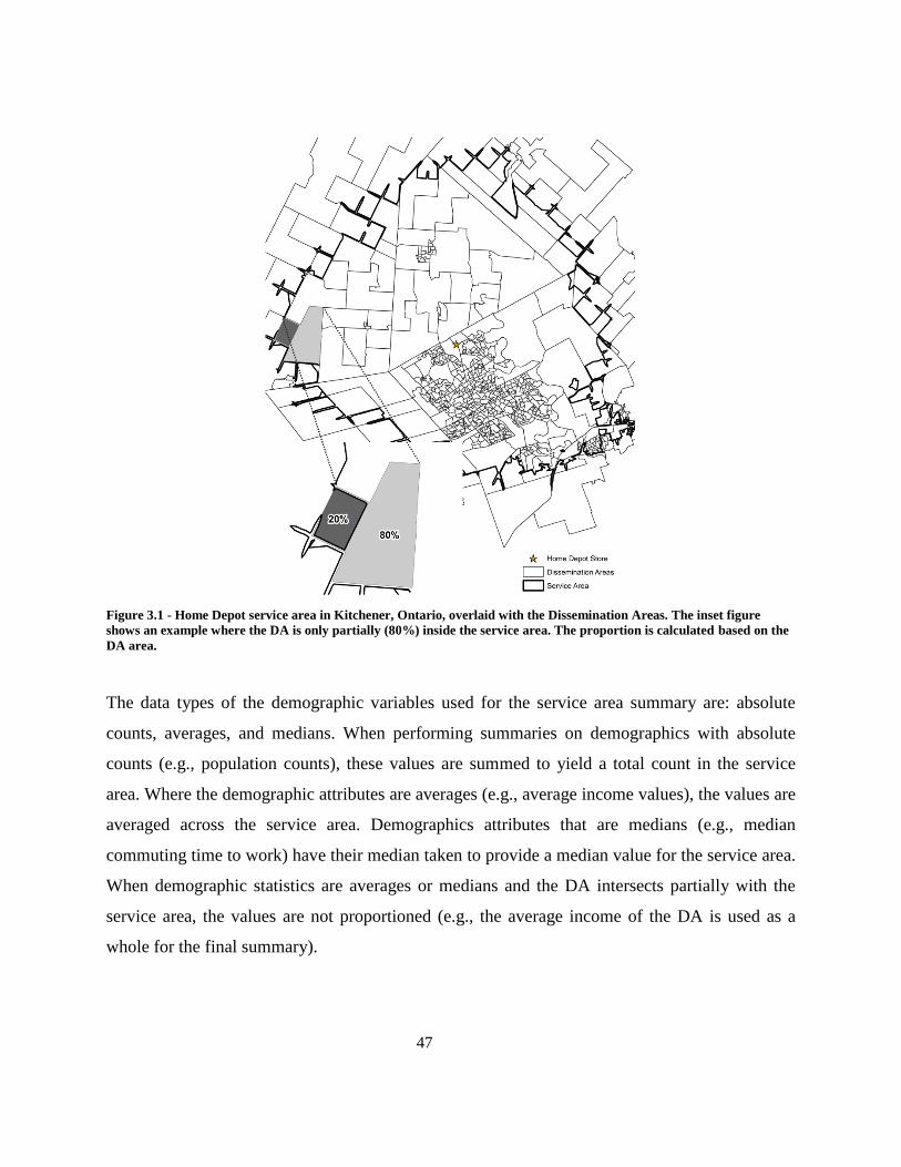
47

Figure 3.1 - Home Depot service area in Kitchener, Ontario, overlaid with the Dissemination Areas. The inset figure

shows an example where the DA is only partially (80%) inside the service area. The proportion is calculated based on the

DA area.

The data types of the demographic variables used for the service area summary are: absolute

counts, averages, and medians. When performing summaries on demographics with absolute

counts (e.g., population counts), these values are summed to yield a total count in the service

area. Where the demographic attributes are averages (e.g., average income values), the values are

averaged across the service area. Demographics attributes that are medians (e.g., median

commuting time to work) have their median taken to provide a median value for the service area.

When demographic statistics are averages or medians and the DA intersects partially with the

service area, the values are not proportioned (e.g., the average income of the DA is used as a

whole for the final summary).

48

The situational characteristics of every store are collected at the time of digitization (Table 3.1).

The competitor count is a total count in the service area of the store. The expenditures variable

is an estimation of market demand for the home improvement sector in Ontario, using the third

method put forward in Chapter Two. When creating the characterization of the chain, these

values are averaged and their standard deviation is calculated. The result is a profile of typical

store formats and competitor attributes of these major chains.

Table 3.1 - Situational store characteristics

Characteristic Description

Retail Area Area (in square feet) of the store footprint

Parking Area Area (in square feet) of the store parking lot

Parcel Area Area (in square feet) of the Ownership parcel the store is located on

Competitor Count Count of Home Improvement stores in the service area

Expenditures Total market demand in the service area for home improvement

The demographic variables selected for characterization are chosen from the 1,431 variables

collected by Statistics Canada in the census and NHS. From these, 930 (65%) are detailed

subdivisions of languages spoken, ethnic origins, and place of birth. A further 196 are detailed

subdivision of general population descriptors (e.g., within family structures, NHS reports

Couples with children, lone-parent with children, female parent, male parent). The remaining

305 characteristics are general demographic descriptors. From these 305 characteristics, 26 were

chosen (Table 3.2) that align with what literature identifies as important demographic groups for

retail (e.g., population and household counts, age, ethnicity, education, labour and income;

Chapter 2, Section 2.5.1). Stepwise regression was used to identify the variables that are

important to store sales.

Table 3.2 – Selected demographic variables for stepwise regression. Percentages in brackets represent the proportion of

the total variable population. Numbers in brackets represent proportion of parent variable population (e.g., for dwelling

type, the parent variable population is all dwellings).

1 Private Dwellings count 14 Dwelling Status: Minor or reg. repair (93%)

2 Population aged 25 to 64 years (55%) 15 Dwelling Status: Major repair (7%)

3 Median age of population 16 Average number of rooms per dwelling

4 Population married/common-law (couple) (58%) 17 Household: Owned (71%)

5 Dwelling type: Detached (single and semi) (61%) 18 Household: Rented (28%)

6 Dwelling type: Apartment (30%) 19 Household maintainers: 1 (58%)

7 Dwelling type: Row (8%) 20 Household maintainers: 2 (39%)

49

8 Average number of persons in household 21 Spending less 30% of income on HH (73%)

9 Immigrants (29%) 22 Average monthly costs (owned shelter)

10 Mobility: Non-movers (previous year) (88%) 23 Average value of dwelling

11 Education: High School and over (81%) 24 Household income: 0 - $100,000 (71%)

12 Labour: Employment rate 25 Household income: over $100,000 (29%)

13 Median commuting duration 26 Median household income

The significant variables identified by the stepwise regression, were summarized for each of the

five chains. For each chain, the average and standard deviation of the significant demographics

for the chain were computed. To identify if there were differences in demographic counts in

proximity to chains as identified by the regression, a one way analysis of variance (ANOVA)

was performed. In order to check the statistical significance of differences in means for the

demographics across chains, the non-parametric Mann-Whitney test was used since the

situational and demographic characteristics are non-normally distributed (assessed with Ryan-

Joiner normality test). The comparisons were performed using a 95% confidence level and

hypothesizing that the means do not differ and that the chains are surrounded by the same

situational and demographic structures.

In addition to the characterization of situational and demographic chain variables, the spatial

distribution of the chains was assessed using the computation of the mean center of the stores,

the count of stores within the first standard deviation from the mean center and the directional

ellipse. These calculations allow for a quantitative description of the chain location patterns

described in terms of their densities and separations (O’Sullivan & Unwin, 2010). The mean

center represents the location which all the stores of a chain are closest to, and can be modeled

using the following equation:

�� = (∑ 𝑥𝑖

𝑛𝑖=1

𝑛,∑ 𝑦𝑖

𝑛𝑖=1

𝑛) (2)

where �� represents the coordinates of the point located at the geographic center of all the stores.

50

Similar to basic statistics, the standard distance calculation is a representation of the deviation of

store locations from their mean center. As this is performed spatially, the equation models the

radius of a standard distance circle from the mean center as follows:

𝒅 = √∑ (𝑥𝑖 − 𝜇𝑥)2 + (𝑦𝑖 − 𝜇𝑦)2𝑛

𝑖=1

𝑛 (3)

where d represents the radius from the mean center (𝜇𝑥, 𝜇𝑦). In a normal distribution, these one,

two and three standard deviation circles should contain 68%, 95%, and 99.7% of the distribution,

respectively. Comparing the proportion of stores contained in a standard distance circle to the

normal distribution value, shows if they are clustered closer to the mean or dispersed.

While the standard distance determines if stores are clustered around the mean center, the

directional ellipse measures the spatial trend of the chain stores by computing the standard

distance for both the latitude and longitude of the mean center. The resulting ellipse identifies if

the store locations have a particular orientation and their spatial spread (Lee & Wong, 2001).

This computation also determines if there is a directional bias (e.g., a chain is spread throughout

southern Ontario only). These spatial statistical methods are important for describing the spatial

patterns of the home improvement chains, as the situational and demographical characteristics

pertain only to the business model and service area market.

2.5 Stores Sales Estimation

The identification of key demographic variables in the service area of a location enables retailers

to understand its quality. However, to test whether a location is optimal in terms of revenues,

retailers can use existing sales as a proxy (Strother et al., 2009). Sales can also be used along

with the characterization of chains to quantify the potential revenues in an area identified as

prime for a retail chain. Since sales at the store level are not reported publicly by retailers and are

available only at the national or (sometimes) provincial level by governments, presenting retail

sales in a city or region for a subsector (e.g., home improvement) is not possible. As such, three

approaches are put forward to estimate store level sales.

51

2.5.1 Approach One: Equal Disaggregation

Retail sales are reported by Statistics Canada in their annual retail store survey at the provincial

level and monthly sales by NAICS subsector at the provincial as well as primary CMA level

(i.e., Toronto). These data are also reported along with the total number of retail stores. A first

approach to estimating store level sales is to equally disaggregate the total sales ($9.687 billion)

by the number of Ontario home improvement stores (3,818). This approach yields a very crude

estimation of sales per store of $2.537 million. Applying this number to each store and

aggregating these values at the Census Subdivision level (i.e., cities) presents the revenue

distribution spatially.

2.5.2 Approach Two: Dollars per Square Foot

The equal disaggregation approach creates a very crude estimation and overestimates the

performance of smaller stores while underestimating the performance of larger stores. Using the

same annual retail survey, the sales by square foot are used to approximate sales given the size of

the store. The visible store area (in square feet) was calculated by computing the area of the store

polygon surface digitized during data capture. Multiplying the sales by square foot value of $286

in Ontario for home improvement from the annual retail store survey in 2011, with each store’s

footprint area yielded an estimation of sales.

While this approach assumes homogeneity in store performance (i.e., every store sells $286 for

every square foot), and typically overestimates and underestimates the performance of smaller

and largeer stores similar to the first approach, this second approach provides a better

approximation than the equal disaggregation, due to the control introduced by the store area.

2.5.3 Approach Three: Mathematical Modelling

Making use of the store area for estimating sales, accounts for the heterogeneity in store size

(i.e., larger stores should yield larger revenues). However, despite their size, some stores perform

52

poorly compared to what the chain and analysts expect. Other variables must be taken into

account beyond the store area when estimating sales. The demographics in close proximity to a

store can be an important descriptor of success, if the chain has located near its target market.

Mathematical modelling software6 was used to fit an equation that estimated sales from the store

area and the collection of demographic variable identified by the regression (section 2.4). This

software is capable of utilizing a variety of mathematical building blocks (e.g., linear,

exponential, trigonometric, logical, regression) to create a model that best fits the data with the

optimal data sets. While all three approaches estimate sales, this third approach was chosen as it

adjusts sales using the store area and demographics (a further optimization than the second

approach).

2.5.4 Assessment of Store Sales

To assess the performance of the third sales estimation approach, two comparisons were made.

Firstly, the aggregate sales of the home improvement stores were compared to the provincial

total of $9.687 billion reported in the annual retail store survey. While the database of home

improvement stores used for this work counts only 1,179 locations and the provincial reported

total is 3,818, it was acknowledge that the aggregate sales should not match the provincial total.

However, as the stores used for this analysis (1,179) represent the major home improvement

chains in Ontario, it was expected that they should account for a majority of the provincial sales.

Secondly, the aggregate store sales in the Toronto CMA were compared to the total $3.543

billion reported in the retail trade monthly sales report provided by Statistics Canada (Statistics

Canada, Table 080-0020). Similar to the first approach, it was acknowledged that the aggregate

sales of the home improvement store database used for this work would not match the total sales

for Toronto, however it should account for the majority of sales.

6 Nutonian’s Eureqa package (http://www.nutonian.com/products/eureqa/) – a machine intelligence software

capable of dynamically deriving mathematical equations from tables of data.

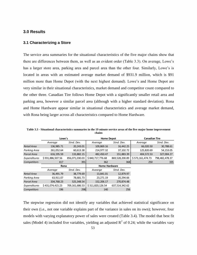
http://www.nutonian.com/products/eureqa/

53

3.0 Results

3.1 Characterizing a Store

The service area summaries for the situational characteristics of the five major chains show that

there are differences between them, as well as an evident order (Table 3.3). On average, Lowe’s

has a larger store area, parking area and parcel area than the other four. Similarly, Lowe’s is

located in areas with an estimated average market demand of $931.9 million, which is $91

million more than Home Depot (with the next highest demand). Lowe’s and Home Depot are

very similar in their situational characteristics, market demand and competitor count compared to

the other three. Canadian Tire follows Home Depot with a significantly smaller retail area and

parking area, however a similar parcel area (although with a higher standard deviation). Rona

and Home Hardware appear similar in situational characteristics and average market demand,

with Rona being larger across all characteristics compared to Home Hardware.

Table 3.3 - Situational characteristics summaries in the 19 minute service areas of the five major home improvement

chains

The stepwise regression did not identify any variables that achieved statistical significance on

their own (i.e., not one variable explains part of the variance in sales on its own); however, four

models with varying explanatory power of sales were created (Table 3.4). The model that best fit

sales (Model 4) included five variables, yielding an adjusted R2 of 0.24; while the variables vary

Average Stnd. Dev. Average Stnd. Dev. Average Stnd. Dev.

Retail Area 136,985.71 20,243.01 109,869.16 16,442.25 66,020.50 30,788.61

Parking Area 261,052.64 60,613.38 214,977.32 37,102.72 125,820.69 54,153.05

Parcel Area 616,195.59 133,882.15 482,450.47 151,883.39 404,572.53 327,004.27

Expenditures 931,886,507.56$ 856,071,030.03 840,717,776.68$ 869,528,200.89 573,161,474.73$ 798,482,478.37

Competitors 417 391 362 368 250 335

Average Stnd. Dev. Avearge Stnd. Dev.

Retail Area 36,491.79 38,779.69 13,841.01 12,879.97

Parking Area 63,911.07 78,681.73 23,271.19 20,294.66

Parcel Area 334,768.23 525,348.54 152,206.17 270,874.48

Expenditures 431,074,415.23$ 709,161,686.53 311,820,126.54$ 637,514,342.62

Competitors 196 298 140 256

Lowe's Home Depot Canadian Tire

Rona Home Hardware

54

in statistical significance (variable influence is significant at varying alpha levels), the overall

model is statistically significant. The same model (Model 4) was identified using an inductive

approach (Appendix C).

Table 3.4 – Four regression models created using the most suitable variables identified by the stepwise regression. (*** p

<0.01, ** p<0.05, * p<0.1)

Variable Description Model 1 Model 2 Model 3 Model 4

Dwelling Counts Count of Dwellings 39.6 47.8* 42.5* 45.3* Income over $100,000 Households with income over $100,000 -338.9* -226.1* -269.6*** -447.5** Immigrants Population identified as immigrant -11.6 -35.8* Dwelling: Owner Count of owned dwellings 32.3 145.5* Average Dwelling Value Value of dwelling in dollars 66.8*** 65.0*** 64.0*** 79.7***

Adjusted R2 0.14 0.16 0.17 0.24

Similar to the situational characteristics of the chain stores, the demographic characteristics

follow the same chain order and reveal differences in values (Table 3.5). Lowe’s and Home

Depot, however, tend to be characterized by very similar demographic counts in their service

areas. The two (on average) have larger demographic counts than Canadian Tire. Rona has on

average smaller demographic counts than Canadian Tire, however larger than Home Hardware.

Table 3.5 - Demographic characteristics summaries in the 19 minute service areas of the five major home improvement

chains

Performing an ANOVA7 to statistically check if the situational and demographic characteristics

of the home improvement chains differ, showed significant differences (α = 0.05; Table 3.6).

Given the extreme f-statistic, the largest difference occurred in the situational characteristics for

7 Calculated using Minitab’s statistical package (http://www.minitab.com/)

Average St Dev Average St Dev Average St Dev

Dwelling Counts 361,342 339,888.43 324,847 343,024.74 223,221 314,978.89

Income over $100,000 89,017 79,793.04 80,554 81,894.85 54,313 75,237.17

Immigrants 397,780 466,582 364,963 461,336 237,520 406,367

Dwelling: Owner 225,886 193,906.55 203,575 199,659.13 138,853 183,331.22

Average Dwelling Value 371,342.43$ 113,177.30 366,128.94$ 118,240.43 322,422.52$ 118,729.22

Average St Dev Avearge St Dev

Dwelling Counts 165,844 273,690.73 125,228 258,647.34

Income over $100,000 41,288 68,603.30 28,390 58,193.00

Immigrants 177,479 357,844 116,512 298,260

Dwelling: Owner 106,642 166,530.89 74,232 140,338.42

Average Dwelling Value 303,692.09$ 110,566.39 289,358.80$ 104,451.58

Lowe's Home Depot

Rona Home Hardware

Canadian Tire

55

the retail and parking area of the chains. The ANOVA findings, justified a further pairwise

comparison of the variables across chains using the Mann-Whitney test8. The pairwise

comparisons of the Mann-Whitney test for the situational (Table 3.7) and demographic (Table

3.8) characteristics help identify which chains differ statistically and which do not.

Table 3.6 - The F-Statistic from the ANOVA for the physical and demographic characteristics. All values significant (α =

0.05). Critical F-value is 2.38.

Table 3.7 - Pairwise comparison p-values from the Mann-Whitney test for chain situational characteristics. All bold

values statistically significant (α = 0.05) while boxed values represent statistically insignificant (similar) values between

chain pairs (LW – Lowes; HD – Home Depot; CT – Canadian Tire; RN – Rona; HH – Home Hardware)

8 Calculated using Minitab’s statistical package (http://www.minitab.com/)

Physical F-Statistic P-Value Demographics F-Statistic P-Value

Retail Area 490.27 0.000 Dwellings Count 13.44 0.000

Parking Area 394.35 0.000 Income over $100,000 16.44 0.000

Parcel Area 38.82 0.000 Immigrants 12.85 0.000

Expenditures 14.83 0.000 Dwelling: Owner 17.28 0.000

Competitors 15.65 0.000 Average Dwelling Value 12.18 0.000

LW HD CT RN LW HD CT RN LW HD CT RN

HD 0.000 HD 0.000 HD 0.000

CT 0.000 0.000 CT 0.000 0.000 CT 0.000 0.000

RN 0.000 0.000 0.000 RN 0.000 0.000 0.000 RN 0.000 0.000 0.000

HH 0.000 0.000 0.000 0.000 HH 0.000 0.000 0.000 0.000 HH 0.000 0.000 0.000 0.000

LW HD CT RN LW HD CT RN

HD 0.269 HD 0.285

CT 0.000 0.000 CT 0.000 0.000

RN 0.000 0.000 0.028 RN 0.000 0.000 0.044

HH 0.000 0.000 0.000 0.012 HH 0.000 0.000 0.000 0.011

Retail Area Parking Area Parcel Area

Expenditures No. of Competitors

56

Table 3.8 - Pairwise comparison p-values from the Mann-Whitney test for chain demographic characteristics. All bold

values statistically significant (α = 0.05) while boxed values represent statistically insignificant (similar) values between

chain pairs (LW – Lowes; HD – Home Depot; CT – Canadian Tire; RN – Rona; HH – Home Hardware)

Comparing the chains’ retail, parking and parcel area for situational characteristics shows that

each chain pair are statistically different (different store sizes across Ontario). For the

expenditures and competitors physical characteristics, Lowe’s and Home Depot are statistically

similar, while the other chains are statistically different. The similarity between Lowe’s and

Home Depot reveals that the two chains are located in areas where there are significantly higher

expenditures available (comparing the means – Table 3.3). Regarding the competitors in the

chain service areas, a conclusive statement cannot be made as the two chains could be locating

near existing competitors (a sign of a good market as explained later) or competitors are

gravitating toward the two chains.

The pairwise comparisons for the demographic variables show that Lowes and Home Depot are

statistically similar across all variables. The statement can be made that the two chains are

located in proximity to very similar markets. The comparisons of the other chain pairs show

statistical difference with the exception of Canadian Tire with Rona, and Rona with Home

Hardware for the average dwelling value demographic characteristic. The two pairs have

statistically similar average values in their service areas. A reason for this similarity could be the

lack of variation in the average dwelling values across the DAs (81% within the first standard

LW HD CT RN LW HD CT RN LW HD CT RN

HD 0.275 HD 0.304 HD 0.323

CT 0.000 0.000 CT 0.000 0.000 CT 0.001 0.001

RN 0.000 0.000 0.028 RN 0.000 0.000 0.023 RN 0.000 0.000 0.033

HH 0.000 0.000 0.000 0.010 HH 0.000 0.000 0.000 0.021 HH 0.000 0.000 0.000 0.019

LW HD CT RN LW HD CT RN

HD 0.287 HD 0.819

CT 0.000 0.000 CT 0.031 0.005

RN 0.000 0.000 0.030 RN 0.003 0.000 0.097

HH 0.000 0.000 0.000 0.011 HH 0.000 0.000 0.002 0.430

Dwelling: Owner Average Dwelling Value

Dwellings Count Income over $100,000 Immigrants

57

deviation) as well as the characterization averaging of the average dwelling values (reduces the

variation further).

Analyzing the spatial distribution of the five major chains reveals that they are situated in

different parts of the province (Figure 3.2). Lowes has a mean center just outside of Toronto (in

Markham) with a directional ellipse spanning from just west of London and east of Central

Frontenac, covering the center of Southern Ontario; 72% of its 29 stores are within its first

standard deviation away from the mean center. Home Depot has its mean center north of Lowe’s

(East Gwillmbury) with a directional ellipse spanning 39% of the 574 Ontario census

subdivisions, having 76% of its 86 stores within the first deviation from the mean center.

Canadian Tire has its mean center in Springwater Township, the second largest directional

ellipse (covering 54% of CSDs), and 74.6% of the 201 stores within the first standard deviation

of the mean center. The mean center of Rona is located in the town of New Tecumseth, the

directional ellipse spans 43% of CSDs (third largest), and 67% of its 132 stores are within the

first standard deviation of the mean center. Lastly, Home Hardware has its mean center furthest

from Toronto (Wasaga Beach), with a larger spread (largest directional ellipse – 55% of CSDs

covered) and 76% of its 427 stores within the first standard deviation from the mean center.

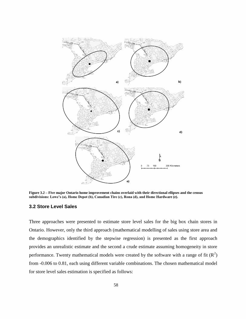
58

Figure 3.2 – Five major Ontario home improvement chains overlaid with their directional ellipses and the census

subdivisions: Lowe’s (a), Home Depot (b), Canadian Tire (c), Rona (d), and Home Hardware (e).

3.2 Store Level Sales

Three approaches were presented to estimate store level sales for the big box chain stores in

Ontario. However, only the third approach (mathematical modelling of sales using store area and

the demographics identified by the stepwise regression) is presented as the first approach

provides an unrealistic estimate and the second a crude estimate assuming homogeneity in store

performance. Twenty mathematical models were created by the software with a range of fit (R2)

from -0.006 to 0.81, each using different variable combinations. The chosen mathematical model

for store level sales estimation is specified as follows:

59

𝑆𝑎𝑙𝑒𝑠 = 26653624.31 + 36.78 ∗ 𝛽 + 4903065.7 ∗ 𝑠𝑖𝑛(0.29 − 𝛾) − 𝛾 ∗ 𝑐𝑜𝑠(𝜃)

− 6815938.03 ∗ 𝑠𝑖𝑛(2.34 ∗ 𝛾) − 3834001.91 ∗ 𝑠𝑖𝑛(3.59 − 5.83 ∗ 𝛾)

where 𝛽, 𝛾, and 𝜃 represent the store area, count of dwellings and households with income over

$100,000. The fit (R2) of this model is 0.79, the correlation of the estimates to actual sales is 0.89

and the mean absolute error is $1,450,308 (4.7% of mean sales).

The home improvement stores in the project database (1,179) had sales estimated using the

mathematical model presented above. The store level sales were aggregated to their containing

CSDs to produce a spatial distribution map of home improvement sales in Ontario (Figure 3.3).

Of the total sales, 68% occurred in the CMAs, where 67% of the home improvement stores are

located. The top three CSDs by sales are Toronto, Ottawa and Hamilton, accounting for 14.7%

of the Ontario home improvement sales.

Figure 3.3 - Ontario CSDs rendered by aggregate home improvement store level sales estimates

60

The Ontario aggregate estimated sales ($31.8 billion) overestimate the provincial reported sales

($9.687 billion) by 228%, with only 31% of all the home improvement stores in the province.

Similarly, the Toronto CMA aggregate estimated sales are 80% larger than the reported sales by

Statistics Canada. As the mathematical model was fit to big-box stores’ sales, it performs poorly

for varying format stores (e.g., for a chain like Canadian Tire), overestimating their sales

significantly.

4.0 Discussion

4.1 Importance of Chain Characterization

The characterization of home improvement chains in Ontario using the situational and

demographic attributes contained in the chain service areas provided a framework for chain

comparison. The service areas are very useful for delineating demographics in close proximity to

a store, as they provide the best representation of the store catchment. Statistically comparing the

averages of the chain demographics identifies similarities and differences between chains. While

it cannot be asserted that these chains seek the identified demographics (from the stepwise

regression) the presence of these values in the service areas allows for the characterization of the

chains.

The two chains with the most similarities (from assessing the means, ANOVA and Mann-

Whitney comparisons for both the situational and demographic variables) are Lowe’s and Home

Depot. These two big-box chains exhibit similarities in store formats, proximity to high market

demand (on average $447 million more demand than the other three chains) and are statistically

similar in the comparisons of demographics in the service areas. The other three chains exhibit

differences in the situational and demographic characteristics, however the chains can be ordered

(by decreasing magnitude of the variables) as Canadian Tire, Rona and Home Hardware. The

61

largest difference between either the situational or demographic characteristics (according to the

ANOVA f-statistic) among the five chains occurs in the store and parking area variables.

Characterizing retail chains using their situational attributes identifies the type of store formats

employed by the chains. While all five chains used for characterization are classified as part of

the home improvement market (NAICS 444), Hernandez (2003) argues that the retail supply of

the home improvement market can be classified as hardware stores, home improvement centers,

and pro dealers. The distinction is primarily made by the products sold by these chains and the

store formats employed (e.g., big-box – over 100,000 square feet). Characterizing Lowe’s and

Home Depot by their situational attributes classifies them as big-box chains (both have average

retail areas over 100,000 square feet, with small standard deviations), while Canadian Tire can

be described as employing different formats (average retail area of 66,000 square feet with a

large standard deviation). This characterization helps identify if a chain is strictly part of retail

supply group or using multiple store formats.

Situational store characteristics address the business model of the retail chains; however,

characterizing chains by the demographics in their service areas is important for a number of

reasons. Firstly, as a chain assesses a location for siting a new store, the demographic

characteristics in the service area of the potential location describe the quality of the market.

Since these chains typically site large format stores, prime locations might not be available close

to dense urban areas, therefore impeding chains from locating in close proximity to their target

market (Grewal, Kopalle, Marmorstein, & Roggeveen, 2012). The demographic characterization

of a location allows a chain to identify what proportion of the service area comprises their target

market. Such an approach helps describe the quality of the market at a proposed location.

Secondly, while a chain could site a store at an optimal location (that satisfies the target market

criteria), the social-economic landscape is considered dynamic, suffering changes over time

(Ghosh & Craig, 1983). This means that a location that was optimal at one point could have a

very different demographic characteristic over a number of years. Evans (2011) argues that a

62

dynamic market should translate to a dynamic retail life cycle that adjusts for demographic

changes. Retail chains can use demographic characterization to assess their markets over time

and adjust accordingly when a location has suffered significant demographic changes.

Lastly, using finer demographic categories (i.e., subdivisions of general descriptors) for chain

characterization can help identify geodemographic segments that are in proximity to chain stores

(Gonzalez-Benito & Gonzalez-Benito, 2005; O’Malley et al., 1997). The segments can be

statistically compared at chain locations where the performance is strong (i.e., high revenues). If

these segments are identified as significant for chain store sales, they can be deemed important

components of the target market for the chain. Using the critical thresholds for these segments

(i.e., average value for a key segment), the landscape can be characterized as optimal or sub-

optimal for a retail chain, identifying spatially what locations the chain should focus on for future

development and expansion.

The characterization approach is important to retailers and municipalities alike. Jones & Doucet

(2000) argue that big-box retailers exert pressures on competitors and the health of the local

retail economy. Specifically for small format chains or hardware stores (as described by

Hernandez, 2003), the characterization of competitors’ service area situational and demographic

variables help identify which portion of the market is challenged by these large chains. While it

cannot be asserted that these are key markets for the large chains, the demographic

characteristics do provide an idea on which segments are likely to shop at these locations.

Municipalities and local governments can also benefit by characterizing the situational and

demographic variables of wanted or unwanted retail chains. If a municipality desires to attract a

chain, by identifying the situational (i.e., store, parking, parcel size) and the demographic (i.e.,

average number of dwellings) chain characteristics, the municipality can assess whether it hosts a

suitable market. In such a case, planning and development policies can be implemented along

with economic incentives to attract such a chain, while outing the presence of a suitable market

for business. A similar approach can be used to assess if the local region is optimal for an

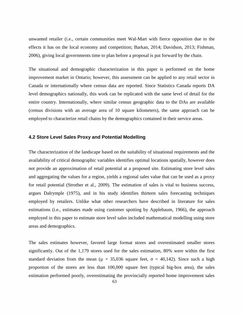
63

unwanted retailer (i.e., certain communities meet Wal-Mart with fierce opposition due to the

effects it has on the local economy and competition; Barkan, 2014; Davidson, 2013; Fishman,

2006), giving local governments time to plan before a proposal is put forward by the chain.

The situational and demographic characterization in this paper is performed on the home

improvement market in Ontario; however, this assessment can be applied to any retail sector in

Canada or internationally where census data are reported. Since Statistics Canada reports DA

level demographics nationally, this work can be replicated with the same level of detail for the

entire country. Internationally, where similar census geographic data to the DAs are available

(census divisions with an average area of 10 square kilometers), the same approach can be

employed to characterize retail chains by the demographics contained in their service areas.

4.2 Store Level Sales Proxy and Potential Modelling

The characterization of the landscape based on the suitability of situational requirements and the

availability of critical demographic variables identifies optimal locations spatially, however does

not provide an approximation of retail potential at a proposed site. Estimating store level sales

and aggregating the values for a region, yields a regional sales value that can be used as a proxy

for retail potential (Strother et al., 2009). The estimation of sales is vital to business success,

argues Dalrymple (1975), and in his study identifies thirteen sales forecasting techniques

employed by retailers. Unlike what other researchers have described in literature for sales

estimations (i.e., estimates made using customer spotting by Applebaum, 1966), the approach

employed in this paper to estimate store level sales included mathematical modelling using store

areas and demographics.

The sales estimates however, favored large format stores and overestimated smaller stores

significantly. Out of the 1,179 stores used for the sales estimation, 80% were within the first

standard deviation from the mean (µ = 35,036 square feet, σ = 40,142). Since such a high

proportion of the stores are less than 100,000 square feet (typical big-box area), the sales

estimation performed poorly, overestimating the provincially reported home improvement sales

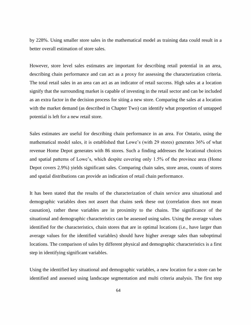
64

by 228%. Using smaller store sales in the mathematical model as training data could result in a

better overall estimation of store sales.

However, store level sales estimates are important for describing retail potential in an area,

describing chain performance and can act as a proxy for assessing the characterization criteria.

The total retail sales in an area can act as an indicator of retail success. High sales at a location

signify that the surrounding market is capable of investing in the retail sector and can be included

as an extra factor in the decision process for siting a new store. Comparing the sales at a location

with the market demand (as described in Chapter Two) can identify what proportion of untapped

potential is left for a new retail store.

Sales estimates are useful for describing chain performance in an area. For Ontario, using the

mathematical model sales, it is established that Lowe’s (with 29 stores) generates 36% of what

revenue Home Depot generates with 86 stores. Such a finding addresses the locational choices

and spatial patterns of Lowe’s, which despite covering only 1.5% of the province area (Home

Depot covers 2.9%) yields significant sales. Comparing chain sales, store areas, counts of stores

and spatial distributions can provide an indication of retail chain performance.

It has been stated that the results of the characterization of chain service area situational and

demographic variables does not assert that chains seek these out (correlation does not mean

causation), rather these variables are in proximity to the chains. The significance of the

situational and demographic characteristics can be assessed using sales. Using the average values

identified for the characteristics, chain stores that are in optimal locations (i.e., have larger than

average values for the identified variables) should have higher average sales than suboptimal

locations. The comparison of sales by different physical and demographic characteristics is a first

step in identifying significant variables.

Using the identified key situational and demographic variables, a new location for a store can be

identified and assessed using landscape segmentation and multi criteria analysis. The first step

65

would necessitate the segmentation of the landscape (e.g., a province) into optimal and

exclusionary areas; these areas would be delineated using the demographic variables that

comprise the target market. The second step would involve the inclusion of other criteria such as

land parcels (to identify locations capable of hosting the desired size of the store) and

topographic features (e.g., sensitive areas, wetlands, highways) into a multi criteria analysis to

identify the most suitable of the optimal areas. Lastly, using demographics as well as

psychodemographic variables, the potential sales at the location would be modeled to understand

the economic sustainability of the store.

4.3 Service Area and Location Based Corrections

Future work on chain characterization and sales estimation should focus on two aspects. First, all

the service areas for the home improvement chains in this study were calculated using the

average 19 minute travel time. While this figure is appropriate for urban areas, travel time from

rural areas to retail stores can be larger. In a study conducted by Gordon & Richardson (1997),

they found that travel from city residents to a store was on average 18.2 minutes, while residents

from outside the city traveled an average of 20.8 minutes. Salonen & Toivonen (2013) modeled

network travel time and found that travel in different parts of the city exhibited varying time

differences. Using alternative travel times for the service areas delineation of chain stores in

urban versus rural areas would yield refined store catchments that would more realistically

summarize the demographic characteristics.

Second, a final modification to sales estimates would be the inclusion of customer satisfaction

data from location based services (LBS) such as twitter feeds. Constantinides, Romero, & Boria

(2008) present a number of methods for using social media and LBS to interact with specific

target market segments. Such an approach would involve harvesting market feedback from social

media and using natural language processing to evaluate the satisfaction with a retail chain (e.g.,

key word “happy” with Home Depot in a tweet). Modeling the satisfaction of the market with the

retail chain and using it as a corrective factor in sales estimations could refine sales values for

66

underperforming chains. The case of the Canadian Target stores and Bennix and Co closing

completely in the past year validates the necessity of such an adjustment.

5.0 Conclusion

The primary goal of this paper was to assess the usefulness of store service areas in identifying

proximal demographic variables from existing store locations and if chain similarities or

differences can be statistically assessed using these variables. Using census data at the finest

geographic resolution available, demographics were summarized for each home improvement

chain store in Ontario, and averages were computed for each chain. These, along with situational

characteristics (i.e., store and parcel areas) were compared using statistical tests and the

significant similarities and differences were assessed.

Big-box home improvement stores tend to have fairly similar physical and demographic

characteristics. While some differences do occur with regards to their formats (i.e. size), the

demographic characteristics were statistically similar for two major big-box chains. When a

chain employs various formats (larger and smaller box types) the physical and demographic

characteristics are statistically different, and while rank can be defined from variable summaries,

no similarities are evident.

A secondary goal was to identify approaches for modeling store level sales from provincial

reports and using demographics. Three approaches were presented, with the chosen approach

being a mathematical model that was fit a function of the store are and select demographic to

actual store sales. As the model was trained using sales of large format stores, and 80% of the

store data used for this work are smaller formats, the sales equation substantially overestimated

smaller store sales

Future work on chain characterization and store sales estimation should focus on three aspects.

First, the separation of big-box and varying format stores is needed within a chain. The results in

this chapter have shown that the comparison of chains employing varying store formats is not

67

appropriate as the underlying assumptions for big-box stores (e.g., products sold, service area

size, situational requirements, revenue generation) are not realistic for varying format stores. To

better assess and compare situational and demographic variables as well as sales across chains,

the store format separation is necessary. Research would necessitate an understanding of small

format store operation, product categories, typical performance (i.e., sales) and chain situational

decisions (why and under what circumstances are small stores opened). Psychodemographic data

for small stores would help focus the demographic characterization.

Second, the dynamicity of travel time to a store in an urban versus rural context needs to be

further investigated. Spatially adjusted travel times will result in more appropriate store service

areas that will more realistically estimate the demographic characteristics. Research on the size

of service area of big-box stores versus a small format stores is also needed. Lastly, location

based services could be used to address the customer satisfaction with a chain. While a sales

estimation approach that adjust for the enterprise size yields results that are less biased to large

format stores, the variation in store performance could be modeled using customer satisfaction.

68

Chapter Four: Conclusion

This thesis has set out to address two aspects of retail location analysis. First, develop a

methodology for estimating retail market demand using consumer expenditures. Since many

retail models require an estimation of market potential (i.e. location-allocation, Huff’s model) for

site suitability evaluation, four methods modeling market demand were put forward. These used

varying data granularity to estimate market demand spatially for Ontario at different census

levels. Spatial analysis was used to identify statistically significant clusters of high expenditures.

These clusters occur in the CMAs where the majority of the population lives and business

activity takes place. Retail stores were identified to gravitate towards clusters of high

expenditures typically being larger in area than stores outside these clusters. Regression analysis

on clusters of high expenditures identified three demographic variables that describe 96% of the

variation in the demand.

The second aspect addressed by the thesis was the creation of an approach to characterize retail

chain stores by situational and demographic variables summarized in the store service areas.

Using statistical comparisons it was established that the five dominant retail chains in Ontario

vary significantly in their characteristics. However, a differentiation was made between what

Hernandez (2003) calls home improvement centers and hardware stores. Big-box chains (with an

average floor space of over 100,000 square feet) showed some similarities in situational

characteristics and statistically significant similarities in the markets found in their service areas.

Chains that employed varying store formats (large and smaller areas) yielded statistically

significant differences both in situational and demographic characteristics. Store level sales were

modeled using the store area and demographic variables; however, as the model was trained on

large format store sales, it overestimated sales for smaller format stores.

1.1 Limitations

The two major limitations encountered during this work were lack of real store sales data and

coarse census data. The mathematical model employed in Chapter Three made use only of a

69

limited number of large format store sales. As such, the model was biased towards larger store

formats in sales estimations. Introducing of a mix of large and small store format sales would

have yielded a more robust estimation model. However, good store sales data are hard to acquire

for two reasons. First, retail chains are particularly careful with sharing sales information. Chan

(2003) detailed that corporate espionage was on the rise due to increased competition, causing

management to introduce fierce controlling measures on employees. Such corporate pressures

make it hard to acquire sensitive sales data even if the purpose is for research. Second, while

business analytics companies (e.g., Hardlines) sell retail information (i.e., chain store details,

sales data), these data are often modeled. As such, the reliability of such data is called into

question when performing retail modelling.

The second major limitation pertains to coarse demographic data presented often only at the

provincial level by Statistics Canada was another major limitation. In their study of estimating

market demand, Strother et al. (2009) had access to household spending categories by income

brackets. This allowed them to match the study area’s median income with the correct income

bracket to use the most appropriate spending values. While Statistics Canada reports, in a similar

fashion, spending by income quintiles (which are significantly different from the income

brackets), many categories especially in the lowest income quintile were suppressed. At the same

time, heavy demographic data suppression at the DA level negatively impacted on of the market

demand estimation methods.

1.2 Implication for Future Research

Future research should specifically address the characterization of retail chain stores by

demographic variables. The work presented in this thesis outlines a framework for identifying

key demographic variables from chain stores’ service areas. Coupled with better store sales

estimates and more demographic descriptors, the service area variables can be identified as

significant when above average values match above average sales. Such an approach is useful for

identifying key demographics around competitors and for characterizing the landscape using the

significant variables to evaluate potential sites where a competitor might locate.

70

Similarly, the framework for market demand estimation and chain characterization put forward

in this thesis can be used to evaluate potential future store closures. Future market demand at a

location can be predicted using spending and income forecasts. Such an assessment could

identify if a location will remain successful in the future; predicted demographic changes or

reduced sales estimates allow a chain to prepare for a change of format or products sold. The

same approach can be used with historic data to assess whether the location was optimal

historically (e.g., higher market demand in the past) and evaluate the changes.

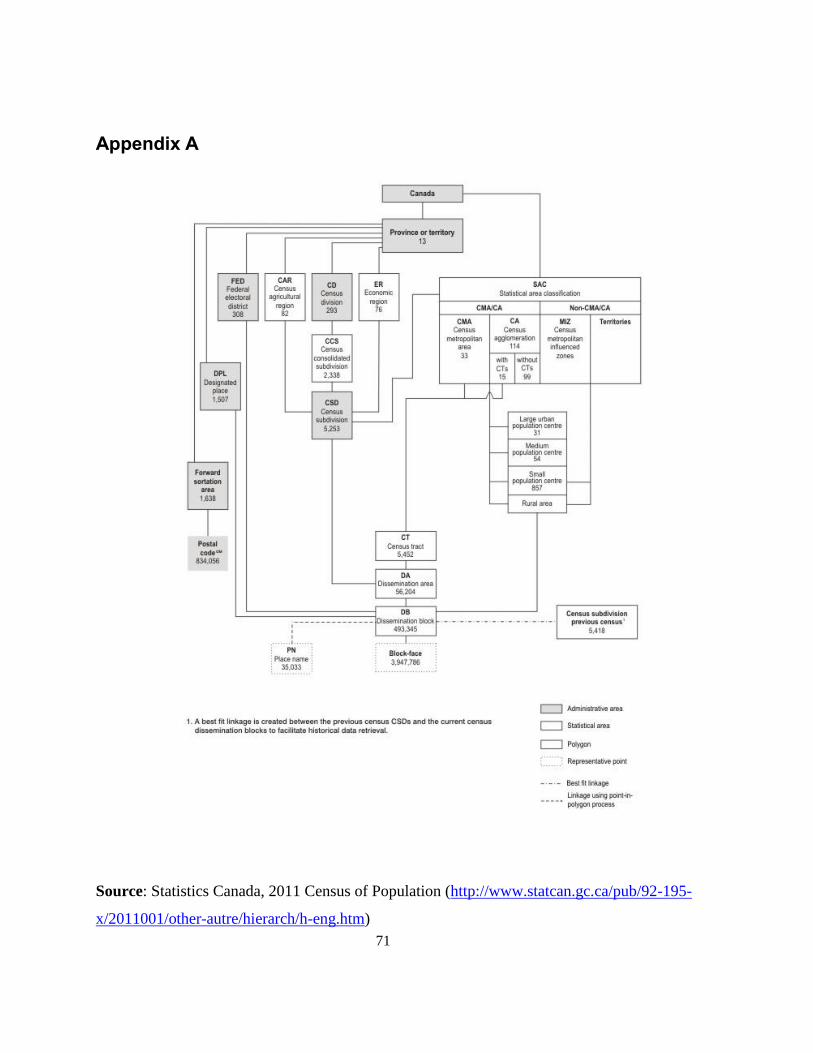
71

Appendix A

Source: Statistics Canada, 2011 Census of Population (http://www.statcan.gc.ca/pub/92-195-

x/2011001/other-autre/hierarch/h-eng.htm)

http://www.statcan.gc.ca/pub/92-195-x/2011001/other-autre/hierarch/h-eng.htm

http://www.statcan.gc.ca/pub/92-195-x/2011001/other-autre/hierarch/h-eng.htm

72

Appendix B

Chain Name Count of Stores Major Competitor*

“Big-box” Chains

1 Home Depot 86 Y

2 Lowes 29 Y

3 Canadian Tire 201 Y

4 Rona 132 Y

5 Home Hardware 427 Y

6 Timber Mart 37

7 TSC Stores 37

8 Sheridan Nurseries 9

9 BMR 7

10 Herman’s 13

Small Chain Formats / Independent Groups

11 Akzo Nobel 51

12 ByTownLumber 4

13 Castle Building Group 71

14 Preston Hardware 1

15 Simcoe Solutions 3

16 Soo Mill Buildall 2

17 TruServ 58

18 Turkstra 11

Total Ontario Stores 1179

* These chains are considered to be dominant in home improvement retail in Ontario,

cumulatively capturing the largest portion of total market share.

73

Appendix C

An inductive approach to variable selection for demographic characterization (Chapter

Three)

The demographic variables selected for characterization were chosen from the 1,431 variables

collected by Statistics Canada in the census and NHS. From these, 930 (65%) are detailed

subdivisions of languages spoken, ethnic origins, and place of birth. A further 196 are detailed

subdivision of general population descriptors (e.g., within family structures, NHS reports

Couples with children, lone-parent with children, female parent, male parent). The remaining

305 characteristics are general demographic descriptors. From these 305 characteristics, 58 were

chosen (Table C1) that align with what literature identifies as important demographic topics for

retail (e.g., population and household counts, age, ethnicity, education, labour and income).

Stepwise regression was used to identify the variables that are important to store sales.

Since stepwise regression uses an automatic combinatorial approach to identify statistically

significant variables, using a large number of predictors significantly increases processing time

and the risk of computer memory errors. In response to this issue, at most 30 variables were

chosen from the 58 as predictors. Also, because some of the 58 variables could be explaining the

same driver of sales (i.e., multicolinearity, which negatively impacts the performance of a linear

regression model), variables were grouped when highly correlated. When a variable is grouped

with another based on the correlation threshold, it must also match the same threshold with every

other variable in that group (Riitters et al., 1995). Since the grouped variables are highly

correlated, choosing any variable from the group should not affect the outcome of the regression.

However, for the presented case study, the most appropriate variable for home improvement was

chosen from each group. When a variable did not group with any other variables, it was counted

as a group on its own and was chosen to go into the regression model.

To identify the appropriate correlation value that would yield at most 30 groups, group counts at

various correlation thresholds were graphed (Figure C1). The three critical values (a significant

difference than expected) occurred at a correlation value of 0.80 (37 groups), 0.70 (30 groups)

74

and 0.4 (16 groups). Since the 0.70 correlation value reduced the set to 30 groups and is also

considered a high correlation, it was chosen as the critical threshold.

Figure C1 - Demographic variables grouping results, using the Pearson's R correlation. The three critical R values are

0.8, 0.7 and 0.4, yielding 38, 30 and 16 groups, respectively, from an initial 58 demographic variables.

The most relevant variable for the home improvement market was chosen from each group (that

had multiple variables; Table C1), and stepwise regression was used to find the model that best

describes sales.

Table C1– Selected demographic variables and correlation groups created by conducting a correlation analysis among 58

demographic variables using a correlation threshold of 0.7

Chosen Variable Count Variables in group

1 Total private dwellings 15

Population in 2011 || Total private dwellings || Married or living with a common-law partner || Not married and not living with a common-law partner || English only || Non-movers || High school diploma or equivalent || Postsecondary certificate, diploma or degree || In the labour force || Not in the labour force || Only regular maintenance or minor repairs needed || Spending less than 30% of household total income on shelter costs || Population aged 25 to 64 years || Population aged 65+ years || Household income: $50,000 - $99,000

2 Median age of the population 1 Median age of the population

3 Average number of children at home per census family

2 Average number of children at home per census family || Average number of persons in private households

4 Owner (Dwelling type) 2 Single-detached house || Owner

5 Spending 30% or more of household total income on shelter costs

5 Apartment, building that has five or more storeys || Renter || 1 household maintainer || Spending 30% or more of household total income on shelter costs || Household income: 0 - $49,000

6 Movable dwelling 1 Movable dwelling 7 Other dwelling 1 Other dwelling 8 French only 1 French only 9 English and French 1 English and French

10 Immigrants 3 Neither English nor French || Immigrants || Asia

11 Household income over $100,000 6 Non-immigrants || Non-immigrants || Employee || 2 household maintainers || Population aged 0 to 24 years || Household income: over $100,000

12 Americas (birth) 1 Americas (birth) 13 Europe (birth) 1 Europe (birth) 14 Africa (birth) 1 Africa (birth) 15 Oceania and other (birth) 1 Oceania and other (birth)

75

16 Movers (Mobility) 1 Movers (Mobility) 17 No certificate, diploma or degree 1 No certificate, diploma or degree 18 Employment rate 1 Employment rate 19 Unemployment rate 1 Unemployment rate 20 Self-employed 1 Self-employed 21 Average weeks worked in 2010 1 Average weeks worked in 2010 22 Median commuting duration 1 Median commuting duration 23 Major repairs needed 1 Major repairs needed 24 Average number of rooms per dwelling 1 Average number of rooms per dwelling 25 Band housing 1 Band housing 26 3 or more household maintainers 1 3 or more household maintainers

27 Average value of dwellings ($) 2 Average monthly shelter costs for owned dwellings ($) || Average value of dwellings ($)

28 Average monthly shelter costs for rented dwellings ($)

1 Average monthly shelter costs for rented dwellings ($)

29 Median household total income ($) 2 Median income ($) || Median household total income ($) 30 Population aged 65+ years 1 Population aged 65+ years

Resulting Model

The stepwise regression model did not identify any variables that achieved statistical significance

on their own (i.e., not one variable explains part of the variance in sales on its own). The model

that best fit sales included five variables (Table C2), yielding an adjusted R2 of 0.24; while the

variables vary in statistical significance (variable influence is significant at varying alpha levels),

the overall model is statistically significant.

Table C2 - Identified demographic variables from the stepwise regression (*** p <0.01, ** p<0.05, * p<0.1)

Variable Coefficient Significance Description

Dwelling Counts 45.26 * Count of Dwellings Income over $100,000 -447.48 ** Households with income over $100,000 Immigrants -35.77 * Population identified as immigrant Dwelling: Owner 145.54 * Count of owned dwellings Average Dwelling Value 79.71 *** Value of dwelling in dollars

76

References

Agrawal, D., & Schorling, C. (1996). Market share forecasting: An empirical comparison of artificial

neural networks and multinomial logit model. Journal of Retailing, 72(4), 383–407.

http://doi.org/10.1016/S0022-4359(96)90020-2

Alon, I., Qi, M., & Sadowski, R. J. (2001). Forecasting aggregate retail sales : a comparison of artifcial

neural networks and traditional methods. Journal of Retailing and Consumer Services, 8(3), 147–

156. Retrieved from http://dx.doi.org/10.1016/S0969-6989(00)00011-4

Anderson, S. J., Volker, J. X., & Phillips, M. D. (2010). Converse’s Breaking-Point Model Revised.

Journal of Management and Marketing Research, 3, 1–10.

Ansuj, A. P., Camargo, M. E., Radharamanan, R., & Petry, D. G. (1996). Sales forecasting using time

series and neural networks. Computers & Industrial Engineering, 31(1-2), 421–424.

http://doi.org/10.1016/0360-8352(96)00166-0

Applebaum, W. (1966). Methods for Determining Store Trade Areas, Market Penetration, and Potential

Sales. Journal of Marketing Research, 3(2), 127–141. http://doi.org/10.2307/3150201

Baltas, G., & Papastathopoulou, P. (2003). Shopper characteristics, product and store choice criteria: a

survey in the Greek grocery sector. International Journal of Retail & Distribution Management,

31(10), 498–507. http://doi.org/10.1108/09590550310497021

Barkan, R. (2014, July 17). Anti-Walmart Coalition Battling Big Box Store at Astoria Cove. New York

Observer. New York City. Retrieved from http://observer.com/2014/07/anti-walmart-coalition-

battling-big-box-store-at-astoria-cove/

Benoit, D., & Clarke, G. P. (1997). Assessing GIS for retail location planning. Journal of Retailing and

Consumer Services, 4(4), 239–258.

Caradima, M. B. (2015). Multi-criteria suitability analysis and spatial interaction modelling of retail

location in Ontario, Canada. Univerity of Waterloo.

Chan, M. (2003). Corporate Espionage and Workplace Trust / Distrust. Journal of Business Ethics, 42(1),

45–58. http://doi.org/10.1023/A:1021611601240

Chu, C.-W., & Zhang, G. P. (2003). A comparative study of linear and nonlinear models for aggregate

retail sales forecasting. International Journal of Production Economics, 86(3), 217–231.

http://doi.org/10.1016/S0925-5273(03)00068-9

Church, R. L. (2002). Geographical information systems and location science. Computers & Operations

Research, 29(6), 541–562. http://doi.org/10.1016/S0305-0548(99)00104-5

77

Clarke, I., Bennison, D., & Pal, J. (1997). Towards a contemporary perspective of retail location.

International Journal of Retail & Distribution Management, 25(2), 59–69.

http://doi.org/10.1108/09590559710160355

Clarkson, R. M., Clarke-hill, C. M., & Robinson, T. (1996). UK supermarket location assessment.


Constantinides, E., Romero, C. L., & Boria, M. A. G. (2008). Social Media: A New Frontier for

Retailers? European Retail Research, 22, 1–28.

Crawford, D. M., & Holt, S. B. . J. (1975). A mathematical optimization technique for locating and sizing

distribution substations, and deriving their optimal service areas. IEEE Transactions on Power

Apparatus and Systems, 94(2), 2–7. http://doi.org/10.1109/T-PAS.1975.31846

Dalrymple, D. J. (1975). Sales Forecasting Methods and Accuracy. Business Horizons, 18(6), 69–73.

http://doi.org/10.1016/0007-6813

Dalrymple, D. J. (1987). Sales forecasting practices: Results from a United States survey. International

Journal of Forecasting, 3(3-4), 379–391. Retrieved from http://dx.doi.org/10.1016/0169-

2070(87)90031-8

Davidson, J. (2013, August 12). Can You Really Keep Walmart Out Forever? Toronto Standard. Toronto.

Retrieved from http://torontostandard.com/the-sprawl/battling-walmart/

Davies, M., & Clarke, I. (1994). A Framework for Network Planning. International Journal of Retail &

Distribution Management, 22(6), 6–10. http://doi.org/10.1108/09590559410070259

Dijkstra, E. W. (1959). A Note on Two Problems in Connexion with Graphs. Numerische Mathematik, 1,

269–271.

Drezner, T. (1994). Optimal continuous location of a retail facility, facility attractiveness, and market

share: An interactive model. Journal of Retailing, 70(1), 49–64. http://doi.org/10.1016/0022-

4359(94)90028-0

Drezner, T. (2010). Cannibalization in a Competitive Environment. International Regional Science

Review, 34(3), 306–322. http://doi.org/10.1177/0160017610389328

Evans, J. R. (2011). Retailing in perspective: the past is a prologue to the future. The International Review

of Retail, Distribution and Consumer Research, 21(1), 1–31.

http://doi.org/10.1080/09593969.2011.537817

Fishman, C. (2006). The Wal-Mart Effect and a Decent Society: Who Knew Shopping Was So

Important? Academy of Management Perspectives, 20(3), 6–25.

http://doi.org/10.5465/AMP.2006.21903477

78

Fox, E. J., Montgomery, A. L., & Lodish, L. M. (2004). Consumer Shopping and Spending across Retail

Formats. The Journal of Business, 77(April 2004), S25–S60. http://doi.org/10.1086/381518

Geurts, M. D., & Kelly, J. P. (1986). Forecasting retail sales using alternative models. International

Journal of Forecasting, 2(3), 261–272. Retrieved from http://dx.doi.org/10.1016/0169-

2070(86)90046-4

Ghosh, A., & Craig, C. S. (1983). Formulating Retail Location Strategy in a Changing Environment.

Journal of Marketing, 47(3), 56–68.

Gijsbrechts, E., Campo, K., & Goossens, T. (2003). The impact of store flyers on store traffic and store

sales: a geo-marketing approach. Journal of Retailing, 79(1), 1–16. http://doi.org/10.1016/S0022-

4359(03)00006-X

Girard, T., Korgaonkar, P., & Silverblatt, R. (2003). Relationship of Type of Product, Shopping

Orientations, and Demographics with Preference for Shopping on the Internet. Journal of Business

and Psychology, 18(1), 101–120. http://doi.org/10.1023/A:1025087021768

Gómez, M. I., McLaughlin, E. W., & Wittink, D. R. (2004). Customer satisfaction and retail sales

performance: an empirical investigation. Journal of Retailing, 80(4), 265–278.

http://doi.org/10.1016/j.jretai.2004.10.003

Gonzalez-Benito, O., & Gonzalez-Benito, J. (2005). The role of geodemographic segmentation in retail

location strategy. International Journal of Market Research, 47(3), 295–316.

Gordon, P., & Richardson, H. W. (1997). Are Compact Cities a Desirable Planning Goal? Journal of the

American Planning Association, 63(February 2015), 95–106.

http://doi.org/10.1080/01944369708975727

Grewal, D., Kopalle, P., Marmorstein, H., & Roggeveen, A. L. (2012). Does Travel Time to Stores

Matter? The Role of Merchandise Availability. Journal of Retailing, 88(3), 437–444.

http://doi.org/10.1016/j.jretai.2012.03.002

Hernandez, T. (2003). Retail restructuring: a geomatics-based analysis of the home improvement sector.

Progress in Planning, 60(1), 35–53. http://doi.org/10.1016/S0305-9006(02)00090-9

Hernández, T., & Bennison, D. (2000). The art and science of retail location decisions The art and science

of retail location decisions. International Journal of Retail & Distribution Managemen, 28(8), 357–

367. http://doi.org/10.1108/09590550010337391

Hernandez, T., Bennison, D., & Cornelius, S. (1998). The organisational context of retail locational

planning. GeoJournal, 45(4), 299–308. http://doi.org/10.1023/A:1006989131869

Hruschka, H. (1986). Market definition and segmentation using fuzzy clustering methods. International

Journal of Research in Marketing, 3(2), 117–134. http://doi.org/10.1016/0167-8116(86)90015-7

79

IHS Global Insight. (2013). The Canadian Home Improvement Products Market by Province.

Washington.

Jones, K., & Doucet, M. (2000). Big-box retailing and the urban retail structure: the case of the Toronto

area. Journal of Retailing and Consumer Services, 7(4), 233–247. http://doi.org/10.1016/S0969-

6989(00)00021-7

Klassen, R. D., & Flores, B. E. (2001). Forecasting practices of Canadian firms: Survey results and

comparisons. International Journal of Production Economics, 70(2), 163–174.

http://doi.org/10.1016/S0925-5273(00)00063-3

Lee, J., & Wong, D. W. S. (2001). Point Descriptors. In Statistical Analysis With ArcView GIS (pp. 33–

57). Toronto: John Wiley & Sons Inc.

Li, Y., & Liu, L. (2012). Assessing the impact of retail location on store performance: A comparison of

Wal-Mart and Kmart stores in Cincinnati. Applied Geography, 32(2), 591–600.

http://doi.org/10.1016/j.apgeog.2011.07.006

Mahmoud, E., Rice, G., & Malhotra, N. (1988). Emerging issues in sales forecasting and decision support

systems. Journal of the Academy of Marketing Science, 16(3-4), 47–61.

http://doi.org/10.1007/BF02723360

Mcdonald, J. F., & Moffitt, R. A. (1980). The Uses of Tobit Analysis. The Review of Economics and

Statistics, 62(2), 318–321.

Mulhern, F. J. (1997). Retail marketing: From distribution to integration. International Journal of

Research in Marketing, 14(2), 103–124. http://doi.org/10.1016/S0167-8116(96)00031-6

Murray, A. T. (2010). Advances in location modeling: GIS linkages and contributions. Journal of

Geographical Systems, 12(3), 335–354. http://doi.org/10.1007/s10109-009-0105-9

Nelson, R. L. (1958a). The Importance of Location Today. In The Selection of Retail Locations (pp. 44–

49). New York: F.W. Dodge Corporation.

Nelson, R. L. (1958b). The Principles of Retail Location. In The Selection of Retail Locations (pp. 50–

56). New York: F.W. Dodge Corporation.

O’Malley, L., Patterson, M., & Evans, M. (1997). Retailer use of geodemographic and other data sources:

an empirical investigation. International Journal of Retail & Distribution Management, 25(6), 188–

196. http://doi.org/10.1108/09590559710175935

O’Sullivan, D., & Unwin, D. J. (2010). Point Pattern Analysis. In Geographic Information Analysis

(Second, pp. 121–154). Hoboken: John Wiley & Sons Inc.

80

Prendergast, G., Marr, N., & Jarratt, B. (1998). Retailers’ views of shopping centres: a comparison of

tenants and non-tenants. International Journal of Retail & Distribution Management, 26(4), 162–

171. http://doi.org/10.1108/09590559810214930

Reynolds, J., & Wood, S. (2010). Location decision making in retail firms: evolution and challenge.


http://doi.org/10.1108/09590551011085939

Rhee, H., & Bell, D. R. (2002). The inter-store mobility of supermarket shoppers. Journal of Retailing,

78, 225–237. http://doi.org/10.1016/S0022-4359(02)00099-4

Riitters, K. H., O’Neill, R. V., Hunsaker, C. T., Wickham, J. D., Yankee, D. H., Timmins, S. P., …

Jackson, B. L. (1995). A factor analysis of landscape pattern and structure metrics. Landscape

Ecology, 10(1), 23–39. http://doi.org/10.1007/BF00158551

Rikalovic, A., Cosic, I., & Lazarevic, D. (2014). GIS Based Multi-criteria Analysis for Industrial Site

Selection. Procedia Engineering, 69, 1054–1063. http://doi.org/10.1016/j.proeng.2014.03.090

Rogers, D. S., & Green, H. L. (1979). A New Perspective on Forecasting Store Sales: Applying Statistical

Models and Techniques in the Analog Approach. Geographical Review, 69(4), 449–458. Retrieved

from http://www.jstor.org/stable/214807

Roig-Tierno, N., Baviera-Puig, A., Buitrago-Vera, J., & Mas-Verdu, F. (2013). The retail site location

decision process using GIS and the analytical hierarchy process. Applied Geography, 40, 191–198.

http://doi.org/10.1016/j.apgeog.2013.03.005

Salonen, M., & Toivonen, T. (2013). Modelling travel time in urban networks: Comparable measures for

private car and public transport. Journal of Transport Geography, 31, 143–153.

http://doi.org/10.1016/j.jtrangeo.2013.06.011

Smith, L. D., & Sanchez, S. (2003). Assessment of business potential at retail sites: empirical findings

from a US supermarket chain. The International Review of Retail, Distribution and Consumer

Research, 13(1), 37–58. http://doi.org/10.1080/0959396032000051684

Statistics Canada, 2011 Census of Population, Canada Post Corporation, May 2011.

Statistics Canada. 2012. Focus on Geography Series, 2011 Census. Statistics Canada Catalogue no. 98-

310-XWE2011004. Ottawa, Ontario. Analytical products, 2011 Census. Last updated October 24,

2012.

Statistics Canada. 2013. Ontario (Code 35) (table). National Household Survey (NHS) Profile. 2011

National Household Survey. Statistics Canada Catalogue no. 99-004-XWE. Ottawa. Released

September 11, 2013. http://www12.statcan.gc.ca/nhs-enm/2011/dp-pd/prof/index.cfm?Lang=E

(accessed April 4, 2014)

81

Statistics Canada. Table 080-0020 - Retail trade, sales by the North American Industry Classification

System (NAICS), monthly (dollars), CANSIM (database). (accessed: 2014-04-04)

Statistics Canada. Table 080-0023 - Annual retail store survey, financial estimates by North American

Industry Classification System (NAICS) and store type, annual (dollars unless otherwise noted),

CANSIM (database). (accessed: 2014-04-04)

Statistics Canada. Table 203-0021 - Survey of household spending (SHS), household spending, Canada,

regions and provinces, annual (dollars), CANSIM (database). (accessed: 2014-04-04)

Statistics Canada. Table 203-0022 - Survey of household spending (SHS), household spending, Canada,

regions and provinces, by household income quintile, annual (dollars), CANSIM (database).

(accessed: 2014-04-04)

Statistics Canada. Table 203-0027 - Survey of household spending (SHS), dwelling characteristics and

household equipment at time of interview, Canada, regions and provinces, annual (number unless

otherwise noted), CANSIM (database). (accessed: 2015-05-12)

Statistics Canada. Table 326-0021 - Consumer Price Index, annual (2002=100 unless otherwise noted),

CANSIM (database). (accessed: 2015-05-15)

Strother, S. C., Strother, B. L., & Martin, B. (2009). Retail market estimation for strategic economic

development. Journal of Retail and Leisure Property, 8(2), 139–152.

http://doi.org/10.1057/rlp.2009.5

Suárez-Vega, R., & Santos-Peñate, D. R. (2014). The use of GIS tools to support decision-making in the

expansion of chain stores. International Journal of Geographical Information Science, 28(3), 553–

569. http://doi.org/10.1080/13658816.2013.858817

Suárez-Vega, R., Santos-Peñate, D. R., & Dorta-González, P. (2012). Location models and GIS tools for

retail site location. Applied Geography, 35(1-2), 12–22. http://doi.org/10.1016/j.apgeog.2012.04.009

Suárez-Vega, R., Santos-Peñate, D. R., Dorta-González, P., & Rodríguez-Díaz, M. (2011). A multi-

criteria GIS based procedure to solve a network competitive location problem. Applied Geography,

31(1), 282–291. http://doi.org/10.1016/j.apgeog.2010.06.002

Tanaka, K. (2010). A sales forecasting model for new-released and nonlinear sales trend products. Expert

Systems with Applications, 37(11), 7387–7393. http://doi.org/10.1016/j.eswa.2010.04.032

Taylor, J. W. (2007). Forecasting daily supermarket sales using exponentially weighted quantile

regression. European Journal of Operational Research, 178(1), 154–167.

http://doi.org/10.1016/j.ejor.2006.02.006

Theodoridis, C., & Bennison, D. (2009). Complexity theory and retail location strategy. The International

Review of Retail, Distribution and Consumer Research, 19(4), 389–403.

http://doi.org/10.1080/09593960903331386

82

Wang, L., & Lo, L. (2007). Immigrant grocery-shopping behavior: ethnic identity versus accessibility.

Environment and Planning, 39(3), 684–699. http://doi.org/10.1068/a3833

Wood, S., & Reynolds, J. (2012). Leveraging locational insights within retail store development?

Assessing the use of location planners’ knowledge in retail marketing. Geoforum, 43(6), 1076–1087.

http://doi.org/10.1016/j.geoforum.2012.06.014

Zotteri, G., & Kalchschmidt, M. (2007). Forecasting practices: Empirical evidence and a framework for

research. International Journal of Production Economics, 108(1-2), 84–99.

http://doi.org/10.1016/j.ijpe.2006.12.004

Estimating retail market potential using demographics and ...

Documents

Transcript of Estimating retail market potential using demographics and ...