Banco de Mexico

Documentos de Investigacion

Banco de Mexico

Working Papers

N◦ 2006-13

Estimating Integrated Volatility Using AbsoluteHigh-Frequency Returns

Carla YsusiBanco de Mexico

December 2006

La serie de Documentos de Investigacion del Banco de Mexico divulga resultados preliminares detrabajos de investigacion economica realizados en el Banco de Mexico con la finalidad de propiciarel intercambio y debate de ideas. El contenido de los Documentos de Investigacion, ası como lasconclusiones que de ellos se derivan, son responsabilidad exclusiva de los autores y no reflejannecesariamente las del Banco de Mexico.

The Working Papers series of Banco de Mexico disseminates preliminary results of economicresearch conducted at Banco de Mexico in order to promote the exchange and debate of ideas. Theviews and conclusions presented in the Working Papers are exclusively the responsibility of theauthors and do not necessarily reflect those of Banco de Mexico.

Documento de Investigacion Working Paper2006-13 2006-13

Estimating Integrated Volatility Using AbsoluteHigh-Frequency Returns*

Carla Ysusi†

Banco de Mexico

AbstractWhen high-frequency data is available, in the context of a stochastic volatility model,

realised absolute variation can estimate integrated spot volatility. A central limit theory en-ables us to do filtering and smoothing using model-based and model-free approaches in orderto improve the precision of these estimators. Although the absolute values are empiricallyattractive as they are less sensitive to possible large movements in high-frequency data, re-alised absolute variation does not estimate integrated variance. Some problems arise whenusing a finite number of intra-day observations, as explained here.Keywords: Quadratic variation, Absolute variation, Stochastic volatility models, Semi-martingale, High-frequency data.JEL Classification: C13, C51, G19

ResumenBajo modelos de volatilidad estocastica, la volatilidad spot integrada puede ser estimada

con la variacion absoluta realizada utilizando datos en alta frecuencia. Dadas las distribu-ciones asintoticas, la precision de estos estimadores puede mejorarse a traves de filtrado ysuavizamiento. A pesar de que el uso de valores absolutos es empıricamente atractivo dadoque son menos sensibles a posibles valores extremos, la variacion absoluta realizada no esun estimador de la varianza integrada. Diferentes problemas pueden presentarse al usar unnumero finito de observaciones intra-dıa como se explica en este documento.Palabras Clave: Variacion cuadratica, Variacion absoluta, Modelos de volatilidad estocasti-ca, Semimartingala, Datos en alta frecuencia.

*I am grateful to Neil Shephard for his constant advice and support. I wish to thank Valentina Corradiand Matthias Winkel for their helpful suggestions.

† Direccion General de Investigacion Economica. Email: cysusi@banxico.org.mx.

1. Introduction

Prices have been recently thought as realisations of continuous time diffusion processes. Completerecords of prices are available for many financial assets at a high-frequency, therefore continuous timemodels can be calibrated. More precisely, within a continuous semimartingale process the sum ofhigh-frequency squared returns estimates quadratic variation. This is why realised variance (the sumof finite squared intra-day returns) can be used as an estimator of integrated variance in a stochasticvolatility model. This result has been extensively studied in the recent literature, e.g. Andersen andBollerslev (1998a), Barndorff-Nielsen and Shephard (2002) and Comte and Renault (1998). Howeverthis is an asymptotic result and infinitesimal returns do not occur in real life. An asymptotic theoryof estimation error was developed to distinguish between true underlying variability and measurementnoise.

Realised variance has been used in financial econometrics for many years, examples include Rosen-berg (1972), Merton (1980), Poterba and Summers (1986), Schwert (1989), Hsieh (1991), Zhou (1996),Taylor and Xu (1997), Christensen and Prabhala (1998), Andersen, Bollerslev, Diebold and Ebens(2001), Andersen, Bollerslev, Diebold and Labys (2001). Recent literature using quadratic varia-tion for semimartingales has been the independently and concurrently development by Andersen andBollerslev (1998a), Comte and Renault (1998) and Barndorff-Nielsen and Shephard (2001). Manyother papers on realised variance exist which are discussed in Dacorogna et al. (2001) and in thereviews by Andersen, Bollerslev and Diebold (2005) and Barndorff-Nielsen and Shephard (2007).

An alternative approach to the realised variance would be using the sum of the absolute valueof the increments of the intra-day log-prices, named realised absolute variation, in order to estimatethe integrated spot volatility of a stochastic volatility model. This is empirically attractive for usingabsolute values is less sensitive to possible large movements in high-frequency data. Taylor (1986)and Ding, Granger and Engle (1993) recognized that empirically absolute returns are more persistentthan squared returns. Andersen and Bollerslev (1997) and Andersen and Bollerslev(1998b) empiricallystudied the properties of realised absolute variation of speculative assets, nevertheless the approachwas abandoned in their subsequent work due to the lack of appropriate theory. Ghysels, Santa-Claraand Valkanov (2003) and Forsberg and Ghysels (2006) retake the interest in absolute returns andprovide empirical and theoretical explanations for the outperformance of realised absolute variation.

Although its empirical advantages, absolute returns (realised absolute variation) have not beenthoroughly studied. Therefore, in this paper, given a stochastic volatility model where the log-pricesare a continuous semimartingale, realised absolute variation is used to estimate the integrated spotvolatility. Following Barndorff-Nielsen, Nielsen, Shephard and Ysusi (2004), the corresponding limittheory will enable us to do filtering and smoothing using a model based and model free approach toimprove the precision of the estimators.

When an underlying continuous process is assumed for the log-prices, the use of high frequencydata to measure volatility can give misleading results because discrete observations are contaminated

1

by market microstructure effects. Although the efficiency of realised absolute variation is measuredwith asymptotic results, using data at the highest available frequency will not necessarily be the bestapproach. Nevertheless, in this paper, we will assume that our observations are not affected by marketmicrostructure noise in order to reach some conclusions; further work is needed to asses the effect ofthis noise in the estimations.

The outline of this paper is as follows. In Section 2 we present some definitions and results forrealised variance and realised absolute variation given in the main literature. We apply the methodsof estimation proposed in Barndorff-Nielsen, Nielsen, Shephard and Ysusi (2004), in Section 3, torealised absolute variation. Finally in Section 4 an analysis about the benefits and faults of usingrealised absolute variation is done following the results in Forsberg and Ghysels (2006). We concludein section 5 and a description of the dataset is given in the Appendix.

2. Framework and properties

A standard model in financial economics is a stochastic volatility (SV) model for log-prices Yt whichfollows the equation

Yt =∫ t

0audu +

∫ t

0σsdWs, t ≥ 0, (1)

where we denote At =∫ t0 audu. The processes σt and At are assumed to be stochastically independent

of the standard Brownian motion Wt. Here σt is called the instantaneous or spot volatility, σ2t the

corresponding spot variance and At the mean process. A simple example of this process is

At = µt + βσ2∗t , where σ2∗

t =∫ t

0σ2

sds.

The process σ2∗t is called the integrated variance.

More generally At is assumed to have continuous locally bounded variation paths and it is set thatMt =

∫ t0 σsdWs, with the added condition that

∫ t0 σ2

sds < ∞ for all t. This is enough to guaranteethat Mt is a local martingale. So the original equation (1) can be rewritten as

Yt = At + Mt.

Under these assumptions Yt is a continuous semimartingale (see Protter (1990)).It is essential to define a discretised version of Yt based on intervals of time of length δ > 0. Given

the previous framework, let the δ-returns be

yj = Yjδ − Y(j−1)δ j = 1, 2, 3, . . . , bt/δc.

Then, independently of the model for the volatility, if At and σt are stochastically independent of Wt,this implies that

yj |aj , ν2j ∼ N(aj , ν

2j ) (2)

2

where aj = Ajδ − A(j−1)δ and ν2j = σ2∗

jδ − σ2∗(j−1)δ. Usually aj is called the actual mean and ν2

j theactual variance.

One of the most important aspects of semimartingales is the quadratic variation (QV), defined as

[Y ]t = p limn→∞

n∑

j=1

(Ytj − Ytj−1)2,

for any sequence of partitions t(n)0 = 0 < t

(n)1 < . . . < t

(n)n = t with supj{t(n)

j − t(n)j−1} → 0 as n → ∞.

As At is assumed to be continuous and of finite variation we obtain that

[Y ]t = [A]t + 2[A,M ]t + [M ]t = [M ]t =∫ t

0σ2

udu

where

[X, Y ]t = p limn→∞

n∑

j=1

(Xtj −Xtj−1)(Ytj − Ytj−1).

This holds since the quadratic variation of any continuous, locally bounded variation process iszero (see Protter (1990)).

The generalisation of quadratic variation is

[Y ][r]t = p limn→∞

n∑

j=1

|Ytj − Ytj−1 |r,

for any sequence of partitions t(n)0 = 0 < t

(n)1 < . . . < t

(n)n = t with supj{t(n)

j − t(n)j−1} → 0 as n →∞.

Now, based on the spot volatility σt, we can define alternatively the integrated spot volatility

σ[1]∗t =

∫ t

0σsds

and the actual volatility

ν[1]j = σ

[1]∗jδ − σ

[1]∗(j−1)δ j = 1, 2, 3, . . . , bt/δc.

It is important to notice that the actual volatility is different from the square root of the actualvariance, so (ν[1]

j )2 6= ν2j .

More about SV models can be found in, for example, Shiryaev (1999) or Shephard (2005).

2.1. Realised absolute variation

The realised absolute variation process is defined as

[Yδ][1]t =

bt/δc∑

j=1

|y|j .

Barndorff-Nielsen and Shephard (2003) derived a limit theorem for the realised power variation

3

process

[Yδ][r]t =

bt/δc∑

j=1

|yj |r,

as δ ↓ 0. Given that realised absolute variation is a special case of realised power variation, r = 1,the asymptotic result can be used to study the properties of the estimation error of integrated spotvolatility.

Barndorff-Nielsen and Shephard (2003) gave the Central Limit Theorem for the realised powervariation process with some restrictive conditions. Barndorff-Nielsen, Graversen, Jacod, Podolskijand Shephard (2005) and Barndorff-Nielsen, Graversen, Jacod and Shephard (2006) provide somegeneral limit results for realised power and bipower variation which are proved under much weakerassumptions.

For the SV model (1) where At is of locally bounded variation,∫ t0 σ2

udu < ∞ and σt is cadlag, wehave that for δ ↓ 0,

µ−1r δ1−r/2[Yδ]

[r]t

p→∫ t

0σr

sds

andµ−1

r δ1−r/2[Yδ][r]t − ∫ t

0 σrsds

µ−1r δ1−r/2

√µ−1

2r υr[Yδ][2r]t

L→ N(0, 1),

where µr = E(|X|r) and υr = V ar(|X|r) with X ∼ N(0, 1).In particular, this implies that

d[Y ][1]t

dt= σt.

From these, we can obtain the relevant result for our case (r = 1) where

√δ

µ1[Yδ]

[1]t

p→ [Y ][1]t

where µ1 =√

2/π, and where √δ

µ1[Yδ]

[1]t − [Y ][1]

t√δ(µ−2

1 − 1)[Yδ][2]t

L→ N(0, 1).

For daily series, suppose there are bt/δc = M intra-h observations during each fixed h time period(here h denotes the period of a day) defined as

yj,i = Y(i−1)h+jδ − Y(i−1)h+(j−1)δ,

for the j − th intra-h return for the i − th period. Then the realised absolute variation, i.e. a scaledsum of the absolute value of the intra-day changes of log-prices, will be defined here as

[YM ][1]i =

1√Mµ1

M∑

j=1

|yj,i|

4

and therefore, [YM ][1]i → σ

∗[1]ih − σ

∗[1](i−1)h when M →∞. So, ν

[1]i = [YM ][1]

i converges to ν[1]i .

Consequently we can use the realised absolute variation as an estimator of the actual volatility.Using the intra-day INTEL prices, the realised absolute variation using five and sixty minutes

returns are plotted, as well as their correspondent autocorrelation functions (Figure 1). As M getssmaller, the series become more jagged. Also, the autocorrelation is higher when the value of M is big,and it shows a slower decay.

0 100 200 300 400 500

0.02

0.04

0.06

0.08

M=78

0 10 20 30 40

0.0

0.2

0.4

0.6

M=78

0 100 200 300 400 500

0.02

0.04

0.06

M=6

0 10 20 30 40

0.0

0.1

0.2

0.3 Acfs: M=6

Figure 1: Realised absolute variation computed using 5 and 60 minutes INTEL returns and their autocorrelation function.

2.2. Realised variance

The realised quadratic variation process is defined as

[Yδ][2]t =

bt/δc∑

j=1

y2j , so as δ ↓ 0 [Yδ]

[2]t

p→ [Y ]t.

For daily series, the realised variance is defined by the summation of the squares of these M intra-period returns and, under semimartingales, as M →∞ then

[YM ][2]i =

M∑

j=1

y2j,i

p→ ν2i = [Y ]ih − [Y ](i−1)h,

5

so the realised variance can be used as an estimator of the actual variance.In Barndorff-Nielsen and Shephard (2002), Barndorff-Nielsen and Shephard (2003) and Barndorff-

Nielsen and Shephard (2004b) the previous theory has been extended to a Central Limit Theorem(CLT). In these papers the CLT is presented under somewhat restrictive assumptions. RecentlyBarndorff-Nielsen, Graversen, Jacod, Podolskij and Shephard (2005) and Barndorff-Nielsen, Graversen,Jacod and Shephard (2006) give weaker conditions on the log-price process which ensure that the CLTholds. For the SV model (1), when δ ↓ 0

δ−1/2([Yδ][2]t − [Y ]t)√

2∫ t0 σ4

sds

L→ N(0, 1),

under the assumptions that At is of locally bounded variation,∫ t0 σ2

udu < ∞ and that σt is cadlag.

0 100 200 300 400 500

0.00

00.

001

0.00

20.

003

0.00

40.

005

0.00

6

M=78

0 10 20 30 40

0.0

0.2

0.4

0.6Acfs: M=78

0 100 200 300 400 500

0.00

00.

001

0.00

20.

003

0.00

40.

005

M=6

0 10 20 30 40

0.0

0.1

0.2

Acfs: M=6

Figure 2: Realised variance series computed using 5 and 60 minutes INTEL returns and its autocorrelation function.

Figure 2 illustrates the time series of realised variances for the INTEL dataset. In the top partof this figure the realised variances and their ACF were computed using M=78, which corresponds tousing five minutes returns data based on the INTEL dataset. The realised variances computed usingM=6, sixty minutes returns, and the correspondent ACF are illustrated in the bottom part of the figure.It can be observed that the realised variance series calculated using five minutes returns (M=78) ismuch less jagged than the series calculated using 60 minutes returns (M=6). The correlograms have

6

the usual slow decay behaviour and it starts at quite a low level for M=6. If we compare the ACF ofthe realised absolute variation with the one of the realised variance, we can notice that the one of therealised absolute variation is marginally stronger.

3. Estimations with Realised Absolute Variation

Absolute returns are well known to have desirable empirical properties, nevertheless further researchis needed about their use as estimators of integrated spot volatility. In this section we will set a modeland estimate integrated spot volatility using realised absolute variation. Barndorff-Nielsen, Nielsen,Shephard and Ysusi (2004) did a similar analysis for realised variance but absolute returns also needto be studied.

When estimating ν[1]i with realised absolute variation, the variance of the error is quite high even

when using large values of M, so a model should be established. A linear model for ν[1]i can be defined

as

ν[1]s:p = cE(ν[1]

s:p) + A[YM ][1]s:p

where

[YM ][1]s:p =

1√Mµ1

(M∑

j=1

| yj,s |,M∑

j=1

| yj,s+1 |, . . . ,M∑

j=1

| yj,p |)′

,

andν[1]

s:p =(ν[1]

s , ν[1]s+1, · · · , ν[1]

p

)′.

We know that√

M

h

([YM ][1]

s:p − ν[1]s:p

)|ν2

s:pL→ N

(0,

(π

2− 1

)Adiag(ν2

s:p)A′)

.

Therefore, we can obtain for the realised absolute variation that

√M

h

(A[YM ][1]

s:p −Aν[1]s:p

)|ν2

s:pL→ N

(0,

(π

2− 1

)Adiag(ν2

s:p)A′)

.

Assuming that the realised absolute variations are a covariance stationary process, the weightedleast square estimator gives in this case that

c = (I − A)ι

A = Cov(ν[1]s:p)

(Cov(ν[1]

s:p) +(π

2− 1

)E(ν2i )h

MI

)−1

.

We can obtain the estimators in a model free or a model based manner. We first look at the modelfree approach.

7

3.1. Sample based method

When using empirical averages, if we have a covariance stationary process of realised absolutevariations and an ergodic daily process, then we know that

1T

T∑

i=1

[YM ][1]i

p→ E(ν[1]i )

and (1T

T∑

i=1

M∑

j=1

y2j,i

)p→ E(ν2

i )

when M and T go to infinity. With these results we can obtain the estimates, as

A =

(Cov([YM ][1]

s:p)−(π

2− 1

)E(ν2i )h

MI

)(Cov([YM ][1]

s:p))−1

.

The Cov([YM ][1]s:p) is easily calculated from the data, and as we are working in daily bases we set h = 1.

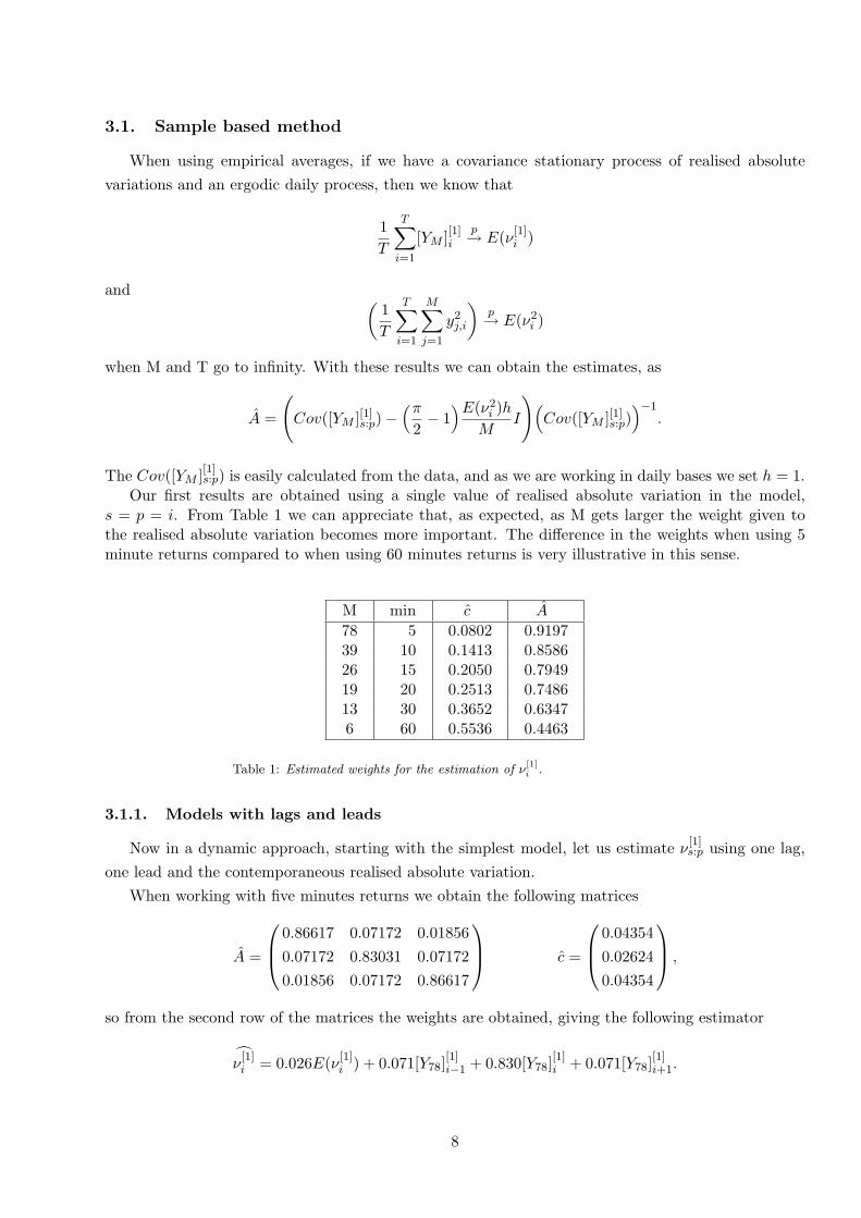
Our first results are obtained using a single value of realised absolute variation in the model,s = p = i. From Table 1 we can appreciate that, as expected, as M gets larger the weight given tothe realised absolute variation becomes more important. The difference in the weights when using 5minute returns compared to when using 60 minutes returns is very illustrative in this sense.

M min c A

78 5 0.0802 0.919739 10 0.1413 0.858626 15 0.2050 0.794919 20 0.2513 0.748613 30 0.3652 0.63476 60 0.5536 0.4463

Table 1: Estimated weights for the estimation of ν[1]i .

3.1.1. Models with lags and leads

Now in a dynamic approach, starting with the simplest model, let us estimate ν[1]s:p using one lag,

one lead and the contemporaneous realised absolute variation.When working with five minutes returns we obtain the following matrices

A =

0.86617 0.07172 0.018560.07172 0.83031 0.071720.01856 0.07172 0.86617

c =

0.043540.026240.04354

,

so from the second row of the matrices the weights are obtained, giving the following estimator

ν[1]i = 0.026E(ν[1]

i ) + 0.071[Y78][1]i−1 + 0.830[Y78]

[1]i + 0.071[Y78]

[1]i+1.

8

Observe that much more weight is given to the contemporaneous realised absolute variation than tothe lag and lead. Nevertheless, if we compare this estimator to the previous one with no lags or leads,less weight is given to the expectation and the weight given as a total to the realised absolute variation(lag, contemporaneous and lead) has increased.

When the realised absolute variation is calculated with sixty minutes returns, the estimator is

ν[1]i = 0.331E(ν[1]

i ) + 0.159[Y6][1]i−1 + 0.349[Y6]

[1]i + 0.159[Y6]

[1]i+1.

Again we can appreciate that as a smaller value of M is used, the less weight is given to the realisedabsolute variation. By using one lag and one lead, the weight in the expectation of ν

[1]i decreases,

and the weight given in total to the realised absolute variation increases compared to the estimationwithout lags or leads, independently of the value of M.

The number of lags and leads can be increased in the model. When using two lags and two leadsfor the estimation, we obtained a 5x5 matrix for A and a 5x1 vector for c. Using their third rows, thefollowing models are obtained when using five and sixty minutes returns consecutively,

ν[1]i = 0.015E(ν[1]

i ) + 0.016[Y78][1]i−2 + 0.062[Y78]

[1]i−1 + 0.826[Y78]

[1]i + 0.062[Y78]

[1]i+1 + 0.016[Y78]

[1]i+2

ν[1]i = 0.253E(ν[1]

i ) + 0.073[Y6][1]i−2 + 0.133[Y6]

[1]i−1 + 0.332[Y6]

[1]i + 0.133[Y6]

[1]i+1 + 0.073[Y6]

[1]i+2

Here, again, the larger the value of M, the bigger the weight given to the contemporaneous realisedabsolute variation. Also, the closer the lags or the leads are to the contemporaneous realised absolutevariation, the bigger the weight given to them. Now, the weights of the unconditional expectation areeven smaller because the actual volatility can be better explained with the lags.

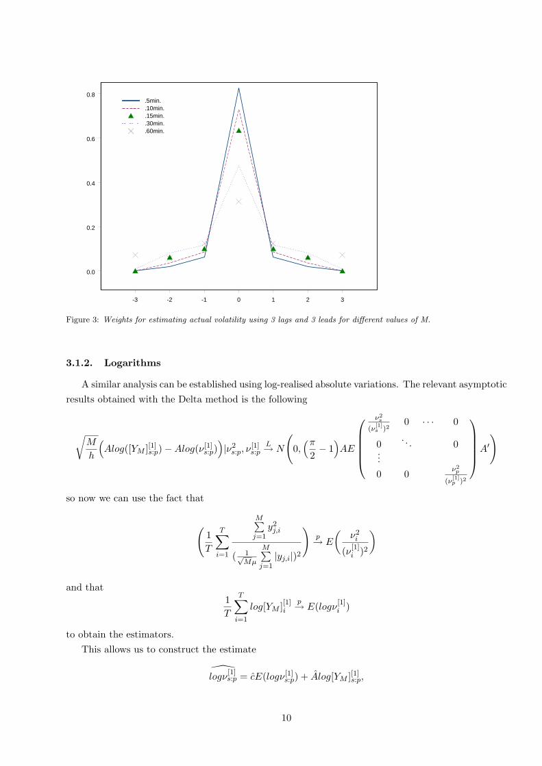
In Figure 3 the weights of a model using three lags, three leads and the contemporaneous realisedabsolute variation are plotted for different values of M. It shows how quickly the weights focus on thecontemporaneous observation of the realised absolute variation as M increases.

9

-3 -2 -1 0 1 2 3

0.0

0.2

0.4

0.6

0.8.5min..10min..15min..30min..60min.

Figure 3: Weights for estimating actual volatility using 3 lags and 3 leads for different values of M.

3.1.2. Logarithms

A similar analysis can be established using log-realised absolute variations. The relevant asymptoticresults obtained with the Delta method is the following

√M

h

(Alog([YM ][1]

s:p)−Alog(ν[1]s:p)

)|ν2

s:p, ν[1]s:p

L→ N

(0,

(π

2− 1

)AE

ν2s

(ν[1]s )2

0 · · · 0

0. . . 0

...0 0 ν2

p

(ν[1]p )2

A′)

so now we can use the fact that

(1T

T∑

i=1

M∑j=1

y2j,i

( 1√Mµ

M∑j=1

|yj,i|)2

)p→ E

(ν2

i

(ν[1]i )2

)

and that1T

T∑

i=1

log[YM ][1]i

p→ E(logν[1]i )

to obtain the estimators.This allows us to construct the estimate

logν[1]s:p = cE(logν[1]

s:p) + Alog[YM ][1]s:p,

10

and given that the realised absolute variations are a covariance stationary process, then the weightedleast squares estimator set

c = (I − A)ι

and

A = Cov(logν[1]s:p)

(Cov(logν[1]

s:p) +(π

2− 1

) h

ME

(ν2

i

(ν[1]i )2

)I

)−1

.

First, by setting s = p = i, i.e. using just the contemporaneous realised absolute variation, andusing logarithms, the results shown in Table 2 are obtained. As before, for smaller values of M used,the weight given to the realised absolute variation gets smaller as well. Compared to Table 1, whenusing logarithms and M is small, higher values for the weight of the log-realised absolute variation arefound. Notice the weights increase just when M is small.

M min c A

78 5 0.0862 0.913739 10 0.1465 0.853426 15 0.2045 0.795419 20 0.2633 0.736613 30 0.3337 0.66626 60 0.4718 0.5281

Table 2: Estimated weights for the estimation of logν[1]i .

When using one lag and one lead in the logarithm model, the same conclusions can be obtained.For five minutes returns we get the model

ν[1]i = 0.032E(logν

[1]i ) + 0.067log[Y78]

[1]i−1 + 0.833log[Y78]

[1]i + 0.067log[Y78]

[1]i+1,

and for sixty minutes

ν[1]i = 0.316E(logν

[1]i ) + 0.101log[Y6]

[1]i−1 + 0.479log[Y6]

[1]i + 0.101log[Y6]

[1]i+1.

In Figure 4 the weights of the log-model using three lags, three leads and the contemporaneousobservation are shown for different values of M. When using logarithms the weights given for smallvalues of M are much higher than those obtained for the estimator based on the raw realised absolutevariation (compare to Figure 3).

11

-3 -2 -1 0 1 2 3

0.0

0.2

0.4

0.6

0.8 .5min..10min..15min..30min..60min.

Figure 4: Weights for estimating log(ν[1]i ) using 3 lags and 3 leads for different values of M.

3.2. Model based estimation

In order to construct a model based estimator of the actual volatility, we need to derive the firstand second moments of ν

[1]i . If ξ is the mean of σt, ω is its variance, and r is its autocorrelation

function, it is known that

E(ν[1]i ) = hξ, V ar(ν[1]

i ) = 2ω2r∗∗h , and Cov{ν[1]i , ν

[1]i+s} = ω2♦r∗∗hs

where

♦r∗∗h s = r∗∗s+h − 2r∗∗s + r∗∗s−h, r∗t =∫ t

0rudu,

and r∗∗t =∫ t

0r∗udu.

So with the second order properties of σt, the second order properties of ν[1]i can be fully established.

In a stochastic volatility model context, realised absolute variation can be written as

[YM ][1]i = ν

[1]i + ui,

so

ui = [YM ][1]i − ν

[1]i =

1√Mµ

M∑

j=1

|εj,i|√

ν2j,i −

M∑

j=1

ν[1]j,i

12

where

εj,iiid∼ N(0, 1)

ν2j,i = σ2∗

(i−1)h+ jhM

− σ2∗(i−1)h+

(j−1)hM

,

ν[1]j,i = σ

[1]∗(i−1)h+ jh

M

− σ[1]∗(i−1)h+

(j−1)hM

,

σ[1]∗t =

∫ t

0σudu and σ2∗

t =∫ t

0σ2

udu.

As stated before√

ν2j,i 6= ν

[1]j,i , so

E(√

Mui|ν[1]i ) 6= 0.

Nevertheless, it is known that√

MuiL→ MN(0, (π

2 − 1)h∫ ih(i−1)h σ2

udu) so

E(√

Mui|ν[1]i ) = o(1).

The second order properties of [YM ][1]i can now be found. First set

E([YM ][1]i ) = E(ν[1]

i ) + E(ui) = hξ +1√M

o(1),

V ar([YM ][1]i ) = V ar(ν[1]

i ) + V ar(ui) + o(1),

Cov([YM ][1]i , [YM ][1]

i+s) = Cov(ν[1]i , ν

[1]i+s) + o(1).

Just V ar(ui) is left to be found to determine these second order properties. Again from the fact that

√Mui

L→ MN

(0,

(π

2− 1

)h

∫ ih

(i−1)hσ2

udu

)

we have that

V ar(√

Mui) =(π

2− 1

)hE

(∫ ih

(i−1)hσ2

udu)

+ o(1)

=(π

2− 1

)h

∫ ih

(i−1)hE(σ2

u)du + o(1)

=(π

2− 1

)h2E(σ2

udu) + o(1)

=(π

2− 1

)h2(V ar(σu) + E2(σu)) + o(1)

soV ar(

√Mui) =

(π

2− 1

)h2(ω2 + ξ2) + o(1).

With these results the variance of the realised variation and its covariance can be established,

V ar([YM ][1]i ) =

(π

2− 1

)h2

M(ω2 + ξ2) + 2ω2r∗∗h +

1M

o(1),

13

Cov([YM ][1]i , [YM ][1]

i+s) = ω2♦r∗∗sh + o(1).

3.2.1. Model

Similar to the realised variance case, for modelling the stochastic volatility, a process with anautocorrelation function as rt = exp(−λ|t|) will be used. The process, which is the solution to thestochastic differential equation

dσt = −λσtdt + dzλt (3)

where zt is a Levy process with non-negative increments, has the previous acf.For this process r∗∗t = λ−2{e−λt − 1 + λt} and ♦r∗∗sh = λ−2(1 − e−λh)2e−λ(s−1)h, s > 0; implying

that the asymptotic moments are

E(ν[1]i ) = ξh,

V ar(ν[1]i ) =

2ω2

λ2(e−λh − 1 + λh)

Cor{ν[1]i , ν

[1]i+s) =

(1− e−λh)2(e−λ(s−1)h)2(e−λh − 1 + λh)

.

The autocorrelation model for the ν[1]i is that one for an ARMA(1,1), so the following linear state-

space representation can be used:

[YM ][1]i = ξh + ( 1 0 )αi + σuυ1i

αi+1 =(

φ 10 0

)αi +

(σσ

σσθ

)υ2i

whereαi = ν

[1]i − ξh and ui = σuυ1i.

Here υi is a zero mean, white noise sequence with an identity covariance matrix; φ, θ, and σσ are theautoregressive root, the moving average root and the variance of the innovation of the process. Finallyσ2

u is found from the asymptotic result for the V ar(ui). The Kalman filter can be used for predictingand smoothing ν

[1]i .

Again, just one of the previous volatility models is too simple to fit the long-range dependencefinancial time series have, so processes will be superposed to describe σu. In this case, we have

σt =J∑

j=1

σ(j)t and

J∑

j=1

wj = 1

where wj are the weights that must be larger or equal to zero and σ(j)t are the processes with memory

λj .Using the previous model ν

[1]i can be estimated for the INTEL dataset. The model was fitted using

five, fifteen and sixty minutes returns, determining the number of processes needed in the superpositionand estimating the parameters.

14

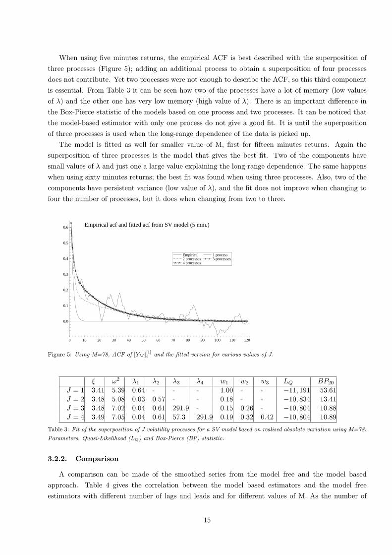
When using five minutes returns, the empirical ACF is best described with the superposition ofthree processes (Figure 5); adding an additional process to obtain a superposition of four processesdoes not contribute. Yet two processes were not enough to describe the ACF, so this third componentis essential. From Table 3 it can be seen how two of the processes have a lot of memory (low valuesof λ) and the other one has very low memory (high value of λ). There is an important difference inthe Box-Pierce statistic of the models based on one process and two processes. It can be noticed thatthe model-based estimator with only one process do not give a good fit. It is until the superpositionof three processes is used when the long-range dependence of the data is picked up.

The model is fitted as well for smaller value of M, first for fifteen minutes returns. Again thesuperposition of three processes is the model that gives the best fit. Two of the components havesmall values of λ and just one a large value explaining the long-range dependence. The same happenswhen using sixty minutes returns; the best fit was found when using three processes. Also, two of thecomponents have persistent variance (low value of λ), and the fit does not improve when changing tofour the number of processes, but it does when changing from two to three.

0 10 20 30 40 50 60 70 80 90 100 110 120

0.0

0.1

0.2

0.3

0.4

0.5

0.6 Empirical acf and fitted acf from SV model (5 min.)

Empirical 2 processes 4 processes

1 process 3 processes

Figure 5: Using M=78, ACF of [YM ][1]i and the fitted version for various values of J.

ξ ω2 λ1 λ2 λ3 λ4 w1 w2 w3 LQ BP20

J = 1 3.41 5.39 0.64 - - - 1.00 - - −11, 191 53.61J = 2 3.48 5.08 0.03 0.57 - - 0.18 - - −10, 834 13.41J = 3 3.48 7.02 0.04 0.61 291.9 - 0.15 0.26 - −10, 804 10.88J = 4 3.49 7.05 0.04 0.61 57.3 291.9 0.19 0.32 0.42 −10, 804 10.89

Table 3: Fit of the superposition of J volatility processes for a SV model based on realised absolute variation using M=78.

Parameters, Quasi-Likelihood (LQ) and Box-Pierce (BP) statistic.

3.2.2. Comparison

A comparison can be made of the smoothed series from the model free and the model basedapproach. Table 4 gives the correlation between the model based estimators and the model freeestimators with different number of lags and leads and for different values of M. As the number of

15

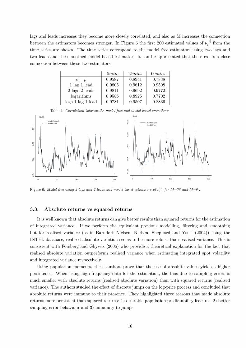
lags and leads increases they become more closely correlated, and also as M increases the connectionbetween the estimators becomes stronger. In Figure 6 the first 200 estimated values of ν

[1]i from the

time series are shown. The time series correspond to the model free estimators using two lags andtwo leads and the smoothed model based estimator. It can be appreciated that there exists a closeconnection between these two estimators.

5min. 15min. 60min.

s = p 0.9587 0.8941 0.78381 lag 1 lead 0.9805 0.9612 0.9508

2 lags 2 leads 0.9811 0.9692 0.9772logarithms 0.9586 0.8925 0.7702

logs 1 lag 1 lead 0.9781 0.9507 0.8836

Table 4: Correlation between the model free and model based smoothers.

0 50 100 150 200

0.01

0.02

0.03

0.04

model basedmodel free

M=78

0 50 100 150 200

0.01

50.

020

0.02

50.

030

0.03

5

model basedmodel free

M=6

Figure 6: Model free using 2 lags and 2 leads and model based estimators of ν[1]i for M=78 and M=6 .

3.3. Absolute returns vs squared returns

It is well known that absolute returns can give better results than squared returns for the estimationof integrated variance. If we perform the equivalent previous modelling, filtering and smoothingbut for realised variance (as in Barndorff-Nielsen, Nielsen, Shephard and Ysusi (2004)) using theINTEL database, realised absolute variation seems to be more robust than realised variance. This isconsistent with Forsberg and Ghysels (2006) who provide a theoretical explanation for the fact thatrealised absolute variation outperforms realised variance when estimating integrated spot volatilityand integrated variance respectively.

Using population moments, these authors prove that the use of absolute values yields a higherpersistence. When using high-frequency data for the estimation, the bias due to sampling errors ismuch smaller with absolute returns (realised absolute variation) than with squared returns (realisedvariance). The authors studied the effect of discrete jumps on the log-price process and concluded thatabsolute returns were immune to their presence. They highlighted three reasons that made absolutereturns more persistent than squared returns: 1) desirable population predictability features, 2) bettersampling error behaviour and 3) immunity to jumps.

16

From this we can conclude that realised absolute variation is a better estimator of integrated spotvolatility than realised variance is of integrated variance. Nevertheless, the main interest is to estimateintegrated variance. Let us compare the asymptotic error distributions for the realised variance processand the squared realised absolute variation process, as well as their logarithmic transformations. Inthe first case we compare

[Yδ][2]t −

∫ t

0σ2

uduL→ MN

(0, 2/δ

∫ t

0σ4

udu)

and ([Yδ]

[1]t

)2−

( ∫ t

0σudu

)2 L→ MN

(0,

4δ

(π

2− 1

)∫ t

0σ2

udu(∫ t

0σudu

)2)

therefore the following inequality needs to hold for absolute returns to give better results than squarereturns,

24(π

2 − 1)

∫ t

0σ4

udu >

∫ t

0σ2

udu( ∫ t

0σudu

)2.

Whether the inequality will hold is unclear, so now we will use a logarithmic transformation where

log([Yδ][2]t )− log

(∫ t

0σ2

udu)

L→ MN

(0,

2δ

∫ t0 σ4

udu)

(∫ t0 σ2

udu)2

)

and

log(([Yδ]

[1]t )2

)− log

((∫ t

0σudu

)2) L→ MN

(0,

4(π2 − 1)δ

∫ t0 σ2

udu

(∫ t0 σudu)2

)

to obtain that2

4(π2 − 1)

∫ t

0σ4

udu >(∫ t0 σ2

udu)3

(∫ t0 σudu)2

.

Again it is unclear whether this is true. But even if it was, we could only say that squared realisedabsolute variation is a better estimator of the squared integrated spot volatility than realised varianceis of the integrated variance. Nevertheless that is not exactly what we are looking for as (

∫ t0 σudu)2

will not always equalise our object of interest,∫ t0 σ2

udu. Therefore we would then need to estimate theintegrated variance with (

∫ t0 σudu)2, adding up an extra error.

Forsberg and Ghysels (2006) also set some regression models to predict ν2t+1 with ν2

t or with ν[1]t .

They obtained a better fit after using ν[1]t as regressor. Ghysels, Santa-Clara and Valkanov (2003)

obtained similar empirical results.Although it is unclear whether realised absolute variation can give better estimations of the inte-

grated variance than realised variance, studies point towards the use of absolute returns rather thansquared returns. Forsberg and Ghysels (2006) and Andersen, Bollerslev and Diebold (2003) studiedbipower variation, introduced by Barndorff-Nielsen and Shephard (2004a), as estimator and predictorof integrated variance and reported that it would improve upon realised variance.

17

4. Conclusions

Given a SV model for the log-prices and the concepts of quadratic and power variation, the avail-ability of high frequency data enabled us to use a time series of realised absolute variation to estimateactual volatilities. When using the raw realised absolute variations as estimator, the errors were largeespecially when M was small. By using the asymptotic distributions of these errors, we improved theestimations via a model based and a model free approach. Both approaches tended to give similarresults when M was large and when several lags and leads were used in the model free estimator.Although absolute values are preferable than squares, realised absolute variation does not estimatethe object of interest, integrated variance, so alternative objects need to be studied as multipowervariation.

5. Appendix: INTEL dataset

Intel stocks are traded on the NASDAQ exchange which predominantly focuses on high technologystocks. The dataset will be constructed from the Trade and Quotes (TAQ) Database. The TAQDatabase is the collection of intra-day trades and quotes for all the securities listed in all the mainUnited States of America equity markets. All this information is available on a collection of CD-ROMs,with each month having between 3 and 10 separate CDs. Further information can be found on theNYSE website (www.nyse.com).

We will work only with transaction prices although a similar analysis can be done based on quotedata. The TAQ database includes each transaction price, but we will take the last recorded priceevery five minutes to have regularly spaced data (last tick method, e.g. Wasserfallen and Zimmer-mann(1985)). We take the prices every five minutes from 9:30 a.m. (when the market opens) until4:00 in the afternoon (when the market closes) for every working day from the first of October of 1998to the twenty-ninth of September of 2000.

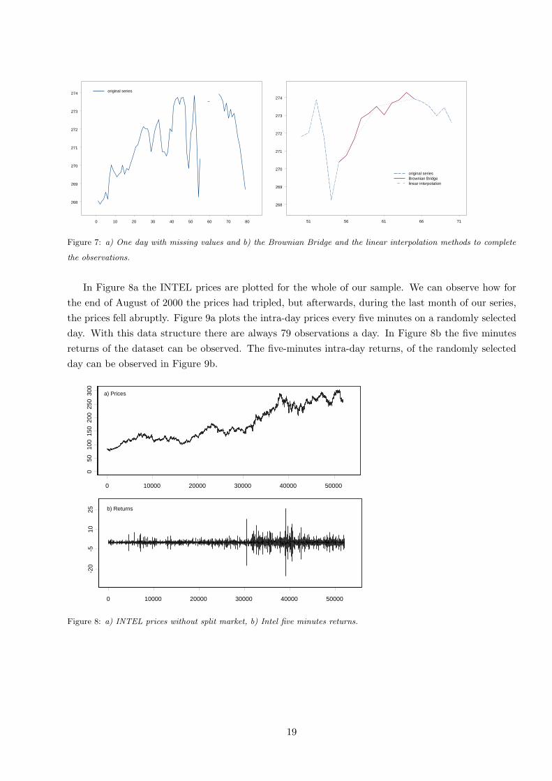
Problems with missing data and split markets can be encountered in this dataset. It consists of39,816 observations (79 observations each day for 504 days), and there are 199 missing values. Thereare just seven days with missing values, and four of them have missing values because the market closedearly that day. To obtain a complete database, a linear interpolation or a Brownian bridge can beused. Figure 7a shows a day with missing values and Figure 7b illustrates both methods (observations56-59 and 61-64 are missing). The problem with the linear interpolation is that the variance of thereturns will be approximately zero for that interval, so we will use a Brownian bridge.

Equity prices used to be decreed by the New York stock exchange to have to be integer multiplesof 1/8 of a Dollar until June 24 of 1997. Afterwards and until January 29 of 2001, they were integermultiples of 1/16 of a dollar. The commission charged by dealers was a fixed number of these ticks.Whenever the price was too high, the percentage of the commission was very small. The Stock Ex-change tried to maintain the prices between ten and one hundred, so when the price was too high, theshare was divided into two half-priced ones. Split markets are not a problem for our work because wecan always multiply the series by two from the day the share was split on. Also we are working withintra-day prices and markets are split at the end of the day, so they do not affect our returns.

18

0 10 20 30 40 50 60 70 80

268

269

270

271

272

273

274original series

51 56 61 66 71

268

269

270

271

272

273

274

original seriesBrownian Bridgelinear interpolation

Figure 7: a) One day with missing values and b) the Brownian Bridge and the linear interpolation methods to complete

the observations.

In Figure 8a the INTEL prices are plotted for the whole of our sample. We can observe how forthe end of August of 2000 the prices had tripled, but afterwards, during the last month of our series,the prices fell abruptly. Figure 9a plots the intra-day prices every five minutes on a randomly selectedday. With this data structure there are always 79 observations a day. In Figure 8b the five minutesreturns of the dataset can be observed. The five-minutes intra-day returns, of the randomly selectedday can be observed in Figure 9b.

0 10000 20000 30000 40000 50000

050

100

150

200

250

300

0 10000 20000 30000 40000 50000

-20

-510

25 b) Returns

a) Prices

Figure 8: a) INTEL prices without split market, b) Intel five minutes returns.

19

10 25 40 55 70108.0

108.5

109.0

109.5

110.0

110.5a) Prices

10 25 40 55 70

-0.005

-0.001

0.003

0.007b) Returns

Figure 9: a) Intra-day prices every five minutes and b) the corresponding intra-day returns of a randomly selected day of

the INTEL series.

20

References

Andersen, T. G. and T. Bollerslev (1997). Intraday periodicity and volatility persistence in financialmarkets. Journal of Empirical Finance 4, 115-158.

Andersen, T. G. and T. Bollerslev (1998a). Answering the skeptics: yes, standard volatility modelsdo provide accurate forecasts. International Economics Review 39, 885-905.

Andersen, T. G. and T. Bollerslev (1998b). Deutsche mark-dollar volatility: intraday activitypatterns, macroeconomic announcements, and longer run dependencies. Journal of Finance 53,219-265.

Andersen, T. G., T. Bollerslev and F. X. Diebold (2003). Some like it smooth, and some like itrough: untangling continuous and jump components in measuring, modelling and forecasting assetreturn volatility. Unpublished paper: Economics Department, Duke University.

Andersen, T. G., T. Bollerslev and F. X. Diebold (2005). Parametric and nonparametric measure-ments of volatility. In Y. Aıt-Sahalia and L. P. Hansen (Eds.), Handbook of Financial Econometrics.Amsterdam: Elsevier Science B.V.

Andersen, T. G., T. Bollerslev, F. X. Diebold and H. Ebens (2001). The distribution of realizedstock return volatility. Journal of Financial Economics 61, 43-76.

Andersen, T. G., T. Bollerslev, F. X. Diebold and P. Labys (2001). The distribution of exchangerates volatility. Journal of American Statistical Association 96, 42-55.

Barndorff-Nielsen, O. E., S. E. Graversen, J. Jacod, M. Podolskij and N. Shephard (2005). Acentral limit theorem for realised power and bipower variations of continuous semimartingales. In Y.Kabanov and R. Lipster (Eds.), From Stochastic Analysis to Mathematical Finance, Festschrift forAlbert Shiryaev. New York: Springer Verlag.

Barndorff-Nielsen, O. E., S. E. Graversen, J. Jacod and N. Shephard (2006). Limit theorems forbipower variation in financial econometrics. Econometric Theory 22, 677-719.

Barndorff-Nielsen, O. E., B. Nielsen, N. Shephard and C. Ysusi (2004). Measuring and forecastingfinancial variability using realised variance with and without a model. In A. C. Harvey, S. J. Koopmanand N. Shephard (Eds.), State Space and Unobserved Component Models: Theory and Applications.Proceedings of a Conference in Honour of James Durbin, 205-235. Cambridge: Cambridge UniversityPress.

Barndorff-Nielsen, O. E. and N. Shephard (2002). Econometric analysis of realised volatility andits use in estimating stochastic volatility models. Journal of the Royal Statistical Society, Series B 64,253-280.

Barndorff-Nielsen, O. E. and N. Shephard (2003). Realised power variation and stochastic volatility.Bernoulli 9, 243-265.

Barndorff-Nielsen O. E. and N. Shephard (2004a). Power and bipower variation with stochasticvolatility and jumps (with discussion). Journal of Financial Econometrics 2, 1-48.

Barndorff-Nielsen, O. E. and N. Shephard (2004b). Econometric analysis of realised covariation:high frequency covariance, regression and correlation in financial economics. Econometrica 72, 885-925.

Barndorff-Nielsen O. E. and N. Shephard (2007). Variation, jumps, market frictions and highfrequency data in financial econometrics. In R. Blundell, P. Torsten and W. K. Newey (Eds.), Advances

21

in Economics and Econometrics. Theory and Applications, Ninth World Congress. Econometric

Society Monographs. Cambridge: Cambridge University Press.Christensen, B. J. and N. R. Prabhala (1998). The relation between implied and realized volatility.

Journal of Financial Economics 37, 125-150.Comte, F. and E. Renault (1998). Long memory in continuous-time stochastic volatility models.

Mathematical Finance 8, 291-323.Dacorogna, M. M., R. Gencay, U. A. Muller, R. B. Olsen and O. V. Pictet (2001). An Introduction

to High-Frequency Finance. San Diego: Academic Press.Ding, Z., C. Granger and R. Engle (1993). A long-memory property of stock market returns and

a new model. Journal of Empirical Finance 1, 83-106.Forsberg, L. and E. Ghysels (2006). Why do absolute returns predict volatility so well? Unpub-

lished paper: Department of Economics, University of North Carolina.Ghysels, E., P. Santa-Clara and R. Valkanov (2003). Predicting volatility: getting the most out of

return data sampled at different frequencies. Journal of Econometrics. Forthcoming.Hsieh, D. (1991). Chaos and nonlinear dynamics: Applications to financial markets. Journal of

Finance 42, 281-300.Merton, R. C. (1980). On estimating the expected return on the market: An exploratory investi-

gation. Journal of Financial Economics 8, 323-361.Poterba, J. and L. Summers (1986). The persistance of volatility and stock market fluctuations.

American Economic Review 76, 1124-1141.Protter, P. (1990). Stochastic Integration and Differencial Equations: A New Approach. New York:

Springer.Rosenberg, B. (1972). The behaviour of random variables with nonstationary variance and the dis-

tribution of security prices. Working paper 11, Graduate School of Business Administration, Universityof California, Berkely. Reprinted in Shephard (2005).

Schwert, G. W. (1989). Why does stock market volatility change over time? Journal of Finance44, 1115-1153.

Shephard, N. (2005). Stochastic Volatility: Selected Readings. Oxford: Oxford University Press.Shiryaev, A. N. (1999). Essentials of Stochastic Finance. Facts, Models, Theory. Advanced Series

on Statistical Science & Applied Probability, Vol. 3. Singapore: World Scientific.Taylor, S. J. (1986). Modeling Financial Time Series. New York: Wiley.Taylor, S. J. and X. Xu (1997). The incremental volatility information in one million foreign

exchange quotations. Journal of Empirical Finance 4, 317-340.Wasserfallen, W. and H. Zimmermann (1985). The behaviour of intraday exchange rates. Journal

of Banking and Finance 9, 55-72.Zhou, B. (1996). High-frequency data and volatility in foreign exchange rates. Journal of Business

and Economic Statistics 14, 45-52.

22