Estimating GDP effects of trade liberalisation on ...

Estimating GDP effects of trade liberalisation on developing countries

Egor Kraev

June 2005 This paper was commissioned by Christian Aid as part of its work on trade policy and developing countries. For more information on Christian Aid’s policy and research work on trade, please contact Claire Melamed on 0207 523 2148

Summary The present project aims to estimate GDP losses caused by trade deficits due to trade liberalisation. Recent econometric studies suggest that while trade liberalisation in poor countries led to an increased growth of both exports and imports, it has caused import growth to systematically outpace export growth (by 1.4 percentage points each year in a sample of 17 Least Developed Countries, and by an even larger margin in a different sample of 22 developing countries). Note that the effect we are studying, namely, import growth exceeding export growth, is not transient, but rather worsens with time, as the difference in export and import growth rates accumulates. Therefore it cannot be fixed by a one-time financing inflow, but rather either by ever-increasing external finance (unrealistic), or by an ongoing depreciation of the real exchange rate. This discrepancy can be expected to cause a worsening of the trade balance, and at the same time a decrease in net demand for domestically produced goods and services, causing a decrease of domestic income (GDP). The allocation of impacts between GDP and the balance of payments in each country and year would depend on private demand and government policy, as well as on the respective country’s ability to raise additional external finance for the increase in trade deficit. The present project aimed to quantify the implications of the econometric studies by using their regression coefficients in a simple macroeconomic model, which was solved for a sample of 32 LDCs and low income countries, once for each year where data was available. The results suggest that over the countries in the sample, trade liberalisation has resulted in additional balance of between 4% and 29% aggregate demand loss (assuming balance of payments unaffected). Converting to constant 2000 US dollars, this sums up to 896 bn USD of aggregate demand losses over a 20-year period. To assess the importance of real exchange rate depreciation in the adjustment to the trade balance deficit, we also conducted sensitivity analysis with respect to real exchange rate changes. The mitigating effect of real exchange rate adjustment never exceeded 25% of the overall impact, and was typically around 10% of the overall impact. That suggests that exchange rate changes alone are not a sufficient adjustment instrument to address trade liberalisation-caused balance of payments problems. The sectors likely to have been most strongly affected by this GDP loss are manufacturing (a sector with most high value-added potential) and the informal service sector (typically containing a large share of the poor). The short-term damage to demand for local manufacturing products is further likely to have led to decreased investment in manufacturing capacity, undermining prospects for future growth.

Estimating GDP effects of trade liberalisation on developing countries

Egor Kraev, Ph.D.1

21. June 2005

Contents

1 Chosen aspect of trade liberalisation 31.1 GDP loss from adverse trade balance effects of trade liberalisation . . . . . . . . . . . 31.2 Other effects I: Financial liberalisation and foreign exchange inflows . . . . . . . . . . 31.3 Other effects II: Supply-side effects . . . . . . . . . . . . . . . . . . . . . . . . . . . . . 4

2 Choice of method 42.1 Computable general equilibrium models . . . . . . . . . . . . . . . . . . . . . . . . . . 42.2 Short-term vs. long-term? . . . . . . . . . . . . . . . . . . . . . . . . . . . . . . . . . . 52.3 A simple variable-output model . . . . . . . . . . . . . . . . . . . . . . . . . . . . . . . 62.4 Specific modeling choices . . . . . . . . . . . . . . . . . . . . . . . . . . . . . . . . . . 7

2.4.1 High aggregation level . . . . . . . . . . . . . . . . . . . . . . . . . . . . . . . . 72.4.2 Foreign exchange inflows are constant across different scenarios . . . . . . . . . 72.4.3 Constant government deficit across scenarios . . . . . . . . . . . . . . . . . . . 72.4.4 Only compare history in a year to counterfactual in the same year . . . . . . . 72.4.5 All accounting is done in dollars . . . . . . . . . . . . . . . . . . . . . . . . . . 82.4.6 Neglect impacts of counterfactual on the real exchange rate . . . . . . . . . . . 8

3 Data 83.1 Selection of countries in the sample . . . . . . . . . . . . . . . . . . . . . . . . . . . . . 93.2 National accounts . . . . . . . . . . . . . . . . . . . . . . . . . . . . . . . . . . . . . . . 93.3 Behavioural parameters . . . . . . . . . . . . . . . . . . . . . . . . . . . . . . . . . . . 93.4 Tariff rates . . . . . . . . . . . . . . . . . . . . . . . . . . . . . . . . . . . . . . . . . . 103.5 ‘First year’ of liberalisation . . . . . . . . . . . . . . . . . . . . . . . . . . . . . . . . . 11

4 Counterfactual Construction 12

5 Results 13

6 Conclusion 16

Appendix

A The Model Equations 16A.1 The accounting framework . . . . . . . . . . . . . . . . . . . . . . . . . . . . . . . . . . 16A.2 Behavioural equations and closure . . . . . . . . . . . . . . . . . . . . . . . . . . . . . 17

B Sensitivity of our results to changes in real exchange rate 19

1Centre for Development, Policy and Research, School of Oriental and African Studies, London; [email protected]

CONTENTS 2

Acknowledgments

The author would like to thank the reviewers of this project, Dr Yilmaz Akyuz, Professor Lance Taylorand Professor John Weeks for their in-depth and insightful comments that allowed the author to correctnumerous deficiencies of the initial and intermediate versions of the model and paper. Needless to say,any remaining deficiencies are the author’s fault.

Introduction

This project aims to estimate GDP losses due to aggregate demand deficiencies arising from tradedeficits due to trade liberalisation. As recent studies [Santos-Paulino 2002a,b, 2003, Santos-Paulinoand Thirlwall 2004], [Unctad 2004, pp.203-204] show, trade liberalisation in poor countries led to anincrease in exports, and to an even higher increase in propensity to import. This led to a worseningof the trade balance, and at the same time a decrease in net demand for domestically produced goodsand services, which likely caused a decrease of domestic income (GDP).

The allocation of impacts between GDP and the balance of payments in each country and yeardepended on private demand and government policy, as well as on the respective country’s ability toraise additional external finance for the increase in trade deficit.

The sectors likely to have been most strongly affected are manufacturing (a sector with most highvalue-added potential) and the informal service sector (typically containing a large share of the poor).The short-term damage to demand for local manufacturing products is further likely to have led todecreased investment in manufacturing capacity, undermining prospects for future growth.

The studies cited above quantify the changes in exports and imports due to lowering of tariffs andremoval of quantitative restrictions. First, we use their regression coefficients to estimate the counter-factual balance of payments, for each country and year, that would be expected to happen had tradeliberalisation not taken place, using historical GDP figures. However, this counterfactual representsan extreme assumption, namely that trade liberalisation had affected the balance of payments, withno impacts on GDP. In reality, especially the poorer countries would likely have difficulties findingextra financing for the increased balance of payments gap (especially once the reforms have been com-pleted). Therefore, most of the impacts of deficient demand caused by trade liberalisation were likelyto have been on GDP.

Thus as the next step, we use the results of Santos-Paulino to construct counterfactual estimatesof GDP levels that could have been sustained from the demand side with historical levels of externalfinancing, had trade liberalisation not taken place. For this, we use a simple injections-leakages modelthat could be regarded as a structuralist counterpart of the neoclassical ‘123’ model [Devarajan et al.1993].

Thus, we construct two ‘extreme’ counterfactuals, one allocating all impacts to the balance ofpayments and leaving GDP intact, the other allocating all impacts to GDP and leaving the balanceof payments intact. In reality, some combination of the two is likely to have happened, with bothbalance of payments and GDP benefits somewhere in the range spanned out by our two estimates.

The following section explains why we think this particular impact of trade liberalisation is worthmodeling and is among the more important aspects of trade liberalisation in poorer countries. Then,Section 2 discusses our choice of method, first in general terms, and then in more detail. Followingthat, Sections 3 and 4 present the data used and the definition of the counterfactuals to be modeled.Section 5 presents the results of the simulations, and Section 6 concludes.

A reader less interested in technical details might want to read Sections 1 and 2.1-2.3 for a discussionof our focus and broad method, and then proceed directly to Sections 5 and 6 for the results.

1 CHOSEN ASPECT OF TRADE LIBERALISATION 3

1 Chosen aspect of trade liberalisation

1.1 Chosen aspect of trade liberalisation: GDP loss from adverse trade balanceeffects of trade liberalisation

The aspect of trade liberalisation that we focus upon is adverse demand-side effects on GDP because ofimport growth exceeding export growth as an effect of trade liberalisation. Although in a typical tradeliberalisation package, both import and export restrictions are removed, typically growth in importdemand exceeds growth in export earnings [Santos-Paulino and Thirlwall 2004, Santos-Paulino 2003],thus leading to a net decrease in overall demand for domestically produced goods and services. This inturn leads to lower income for domestic producers, lower GDP and hence lower import demand; thusbalance of payments is maintained, but at a lower level of GDP. The impact on GDP is strengthenedby the multiplier effects.

It is sometimes argued that this is only a temporary phenomenon, to be remedied by one-offexternal financing, but it is not clear why it should be so (there is certainly no reason to be found ingeneral equilibrium theory, as discussed in Section 2.2). If trade liberalisation leads to an increase inimport demand that exceeds the corresponding increase in exports, the result will be either a persistentincrease in trade deficit or a permanent reduction in GDP. If, as the regressions in [Santos-Paulino andThirlwall 2004, Santos-Paulino 2003] suggest, trade liberalisation actually affects the rates of growthof exports and imports in an asymmetrical manner (increasing the yearly rate of growth of exports by0.5% and of imports by 1.9% for a sample of 17 least-developed countries (LDCs) in Santos-Paulino[2003]), then the gap, though small at first, will actually be widening with every year, as long as thatrelationship holds.

Thus, there is no reason to expect the effect to be temporary, and a gap in growth rates of1.4% between exports and imports, when cumulated over several years, is likely to produce resultsof noticeable magnitude. This is the effect that we will be aiming to quantify; however, this is notthe only important aspect of a typical trade liberalisation package. Therefore, before proceeding todiscuss modeling approaches, we discuss its relationship to the other important components. Of these,there are two broad groups, one to do with financial liberalisation and capital account dynamics, theother with supply-side effects. Let us discuss each in turn.

1.2 Other effects I: Financial liberalisation and foreign exchange inflows

Trade liberalisation has historically often been accompanied by liberalisation of the capital account,that is removal of restrictions on the movement of capital into and out of the country. Many countriesthat liberalised their trade as part of an International Monetary Fund-inspired structural adjustmentpackage, have additionally been rewarded with increased concessional inflows, at least for a while(Ghana in the late 1980s is a prominent example of the latter).

As increased external inflows can compensate for aggregate demand deficiency caused by a wors-ening balance of payments position (in particular, it has been argued that more liberalised countriesreceive more external finance), one might be tempted to think that the latter is not a major problemand does not deserve the attention we are about to give it.

We would argue that this is not the case. As discussed in the previous section, there is no reason toassume the balance of payments gap due to trade liberalisation will go away after a year or two, thussuch a compensating foreign exchange inflow would need to be sustained from year to year. This rulesout the possibility of using grants for the purpose, as the grant flows are notoriously volatile. However,any form of sustained foreign borrowing, be it concessional or private, will lead to debt buildup andthus even greater balance of payments problems in the future (Ghana being again the case in point).The remaining option is foreign direct investment, which is generally quite low for poorer countries.

Financial liberalisation is an important subject in itself. It has often led to inflows of speculativecapital, driving up exchange rates, thus further worsening the current account (‘Dutch Disease’). Incountries with comparatively well developed banking systems, particularly in Asia and Latin America,

2 CHOICE OF METHOD 4

the credit inflows have also often resulted in boom-bust credit cycles.The impact of financial liberalisation has been quite different across developing countries, de-

pending among other things on the depth of the domestic financial sector and its importance in theeconomy. The present inquiry focuses on LDCs and countries of sub-Saharan Africa, where bankingsystems are comparatively shallow and private capital inflows comparatively modest. Therefore, mostof the action on the capital account was due to donor decisions. Thus, even if it was true for thosecountries that countries that liberalised further also experienced higher capital inflows, these two com-ponents are conceptually distinct and deserve to be considered separately. If external inflows are afunction of donor policy, they should be treated as policy variables and not endogenized.

1.3 Other effects II: Supply-side effects

Another important facet of trade liberalisation are its supply-side effects, that is effects on the stockof productive capital and the structure of production. These can be roughly divided into quantitative(amount of new investment) and qualitative (technological innovation, improved productivity, etc.).

The effects of trade liberalisation on investment will have profound effects on the productivecapacity of the economy in the future. Unfortunately, investment is notoriously hard to model, evenin industrialised countries with their comparative data abundance, and even more so in developingcountries.

In the absence of robust regressions, one has to rely on case studies and qualitative stories. These,however, also contradict each other. On the one hand, one has the promise of increased efficiency inimport-competing industries and new investment in exportable goods due to improved incentives; onthe other hand, a number of studies indicate that investment is hit quite hard by a number of compo-nents of a typical liberalisation package, from decreased aggregate demand to high interest rates andincreased competition from cheap imports. The qualitative effects such as technological innovationare even harder to assess.

Summing up, in this paper we focus on adverse GDP effects of balance of payment deficits causedby trade liberalisation, under conditions of scarce access to foreign exchange. While capital accountdevelopments and supply-side effects are also extremely important, the former are conceptually distinctfrom trade policy in the case of poorer countries; and the latter are somewhat contested and lackrobust quantification. Thus while our results will not be comprehensive, they will give a picture ofan important component of trade liberalisation impacts for those countries and time periods wherescarce access to foreign exchange is a valid assumption.

2 Choice of method

2.1 Computable general equilibrium models, neoclassical and otherwise

To quantitatively address our question, we need a widely accepted methodology that allows us tocombine individual behavioral equations with comprehensive economy-wide accounting.

The methodology most often used for this purpose are computable general equilibrium models(CGEs). A CGE takes the data on a given economy’s money and product flows, combines these witha priori assumptions on causal mechanisms in that economy and gives one the implications thereof. Ifthe causal structure we assume (also known as choice of closure) is a good description of the economyat hand, the model output will be credible. A CGE does not itself allow us to verify the assumptionsthat went into it, but it does allow us to quantify their implications.

The use of CGEs for policy analysis is controversial because there is no consensus on the appropriateassumptions to make. Thus, for example, the model by Sahn et al. [1996] cited in the 2004 UNConference on Trade and Development (Unctad) LDC report was harshly criticised by de Maio et al.[1999] as using assumptions that were not appropriate to the economies being modeled.


The mainstream thinking on impacts of trade policy is deeply influenced by the Heckscher-Ohlininternational trade model, whose key assumptions are automatic full employment, frictionless relo-cation of productive capacity between exports and nontraded goods (albeit subject to diminishingreturns), and balanced trade (no trade deficits). Under such conditions, it is easy to demonstrate thatincreased trade will have net beneficial impacts for all involved.

This line of argument is continued by Walrasian/neoclassical CGE models, which no longer nec-essarily assume balanced trade, but still rely for their conclusions on automatic full employment andfrictionless relocation of productive capacity between sectors. The simplest of such models is the‘123’ model by Devarajan et al. [1993]. Its name stands for ‘one country, two sectors (nontraded andexported) and three goods (exports, imports and nontraded goods)’. Its simplicity allows it to becalibrated using only national accounts data and a couple of key elasticities, and it was for a whilemuch promoted by the World Bank as an entry-level CGE model for use by the developing countries.

Unfortunately, ‘123’ is a typical Walrasian model in that it assumes automatic full employmentthroughout. The importance of that one assumption in determining the behaviour of the model can notbe overemphasized. For example, in a Walrasian model an increase in export production will only bepossible by relocating some labour from the nontraded goods production, thus an increase in exportsmust be associated with a decrease in nontraded goods production. On the other hand, if production ofnontraded goods were demand-driven, with variable utilization of productive capacity, then increasedincome from exports would translate into higher demand for consumption and investment goods, inparticular nontraded ones, leading to an increase in nontraded goods production.

Thus, before using a model for drawing policy conclusions, it is crucial to decide whether it shallinclude the full employment assumption.

2.2 Short-term vs. long-term?

The usual neoclassical argument regarding the full employment assumption is that it can be expected toprevail in the ‘long term’, once the short-term shocks have been adjusted to. However, this statementis in conflict with persistent evidence of chronic unemployment in many developing countries, and(perhaps a little more surprisingly) also in conflict with general equilibrium theory. If one goes backto read the general equilibrium classics such as Arrow [1974], one sees that full employment is onlyguaranteed if there are functioning futures markets for all commodities contingent on all possiblefuture states of the world (so that it is, for example, possible to have a contract to buy a loaf ofbread tomorrow, but only if it rains); since the majority of such markets are neither existing nor evenfeasible, there is absolutely nothing about the ‘long-term’ that guarantees full employment of eitherlabour or capital [Kraev 2003].

The justification of full employment as a ‘long-term’ property is even less defensible if the CGEmodel in question is expanded to include accumulation of capital and financial stocks and then re-solved on a yearly basis - how can the long term obtain over a year’s time?

In reality, developing countries are continually subjected to shocks, both external and internal,such as changes in price of their exports or in government policy. This, together with evidence ofpersistent unemployment and underemployment, leads us to conclude that an adequate CGE modelof a developing country must allow for variable utilization of productive capacity.

In fact, once the full employment (or rather, fixed output) assumption is no longer built in, ourmodel (presented in the next section) can be used to test it – and the data suggests, once again, thatit does not hold, even after taking into account exchange rate response (Appendix B).


2.3 A simple variable-output model

We will estimate the costs of trade liberalisation by solving a very simple computable general equi-librium model2 built along structuralist lines, for each country and each year where data is available.The model will have a variable-output closure (injections/leakages equilibrium) formulation followingGodley and Cripps [1983] and Berg and Taylor [2000]

We take essentially the same accounting framework that the ‘123’ model uses (one country, twosectors, three goods), but modify its closure to allow for variable capacity utilization. Another sim-plification we make is doing all accounting in dollars, thus allowing us to sidestep domestic inflationissues. This does not introduce a theoretical weakness, since in ‘123’, as in all Walrasian models, thenominal aggregate price level is tacked on top of the model and does not affect the real-side variables(this is, in fact, the exact approach chosen by Devarajan and Lewis [1990]).

The details are written out in Appendix A, but the basic story of the model is simple enough.Namely, suppose that tariffs change relative prices of exports and imports compared to the domesticgoods, which changes export and import volumes. That leads to an imbalance in the balance ofpayments due to a higher increase in the demand for imports than in export revenue. This translatesinto a lower overall demand for domestic goods, and as a large part of any economy is demand-driven, that leads to a decrease in GDP. As a result, import demand also declines, bringing balanceof payments back into balance.

The crucial points of that story are the choice of variable-output (or quantity-clearing) closure, thatis, taking the main adjusting variables to be (nontraded) output on the income side and consumptionor investment on the expenditure side; and an external financing constraint, that prevents unlimitedborrowing to cover the trade balance deficits. The first of these we have discussed in the previoussection; the second we elaborate upon in Section 2.4.2. Our model is in fact a variant of two-gapmodels (reviewed in Taylor [1994]), with the trade account as the ‘binding gap’.

An additional choice we make is to calibrate the model and conduct experiments separately foreach year rather than simulate the same model across several years. This allows us to omit from themodel equations many factors, such as world prices, that differ between years and matter for modelbehaviour, but are unaffected by our counterfactual experiments. We can thus obtain a particularlylightweight model formulation that would not be useful for addressing some other issues such as debtaccumulation, but is perfectly adequate for our question, namely negative effects of liberalisation-caused balance of payments deficits on GDP.

A neoclassical/Walrasian model would seek to avoid quantity effects (such as GDP decreases) al-together by adjusting relative prices, notably the real exchange rate. However, all Walrasian modelsassume automatic full employment, and thus are fundamentally unable to represent the very recession-ary impacts that we are trying to estimate. Also, the role of real exchange rate as the clearing variablefor the balance of payments is not supported by data (at the very least, one has to include portfoliobalance considerations; and [Taylor 2004, ch.10] argues that even this will not work). Thus, we feelthat allowing for variable capacity utilization is more important than endogenizing (in an unrealisticmanner) the real exchange rate. The issue is discussed in more detail in Section 2.4.6.

Summing up, while more sophisticated models would be possible, even using the same data, ourchoice of approach is caused by two factors: firstly, the model used must be so simple as to betransparent, so that the debate can focus on the policy implications rather than on the model details.Secondly, its equations must not a priori preclude impacts of changes in tariff rates on real GDP,which means that traditional Walrasian/neoclassical formulations are not useful. Thus, our minimaldemand-driven model appears to be the best solution for the task at hand.

The following section discusses and justifies in some more detail some of the specific modelingchoices we make.

2Since our closure is quantity- rather than price-clearing, one might argue that it is not a “proper”, meaning Walrasian,CGE. We believe that this is a purely linguistic issue, and the approach can be called a quantitative analytical frameworkinstead if it doesn’t fit the reader’s idea of what a CGE should be.


2.4 Specific modeling choices

This section begins the more technical part of the paper. The less technically inclined reader mightwant to skip directly to Section 5, Results.

2.4.1 High aggregation level

The model stays at the macro level, with the same sectoral/product structure as the ‘123’ model,namely 2 sectors (nontraded and export) and 3 goods (imports, nontraded goods and exports). Theadvantage of that is that we need little beyond the standard national account and balance of paymentsdata to calibrate the model. As that data is available for most countries and most years, we can achievebroad coverage.

The disadvantage of staying at this level of disaggregation is that it does not capture the sectoraland distributional impacts of trade liberalisation. As rough sectoral output data is also broadly avail-able, it would be conceivable to include some sectoral structure in the future; however, for pragmaticreasons we restrict ourselves to capturing purely macro impacts at present.

2.4.2 Foreign exchange inflows are constant across different scenarios

While liberalisation programmes in the countries that we are looking at (LDCs, low income and sub-Saharan Africa countries) have often been associated with extra capital inflows, the two are concep-tually separate phenomena, and it makes sense to consider them separately, especially as concessionalinflows are a function of deliberate donor policy, not spontaneous private sector dynamics.

The precise question our model is answering is ‘How large a GDP level could have been sustainedfrom the demand side, given historical lending flows, if the balance of payments impacts of tradeliberalisation had not happened?’. Thus, this assumption is not necessarily indicative of a foreignexchange strangulation, but rather of the particular counterfactual that we are constructing.

In addition, we construct a complementary counterfactual, namely assuming the GDP was unaf-fected and computing the pure balance of payments impacts. In reality, the impacts would likely havebeen a combination of the two.

2.4.3 Constant government deficit across scenarios

As a result of trade liberalisation, revenues from export and import tariffs are likely to fall; as a resultof the adverse GDP impact, revenue from taxes such as VAT and income tax is also likely to fall.Thus, in addition to the GDP impact, our framework computes the reduction in government revenuesthat will translate either into increased deficit or reduced government spending.

In the current version of the model, we assume that spending is adjusted in line with revenues soas to keep deficit constant. This is not unrealistic: most countries liberalised their trade as a part ofan IMF package, the performance conditions of which were likely to include constraints on governmentdeficit, so that spending will have to be reduced in line with revenues.

However, this is not as critical to the model formulation as the foreign exchange constraint. Sinceours is a flow-only framework, if the government runs a deficit, it will have to borrow from theprivate sector, correspondingly reducing its demand. Thus, given the balance of payments constraint,government deficit only determines the allocation of absorption between government and the privatesector; we could just as easily assume that the government fixes its spending and interpret the reductionin revenues as an increase in government deficit rather than as a decrease in spending; the GDP impactswouldn’t be affected.

2.4.4 Only compare history in a year to counterfactual in the same year

In real life, changes in government deficit in a year result in changes in government debt and thereforeinterest payments the following years (though a large part of these deficits in LDCs are closed by

3 DATA 8

budgetary grants which do not lead to debt accumulation). However, we do not keep track of that,because we construct a separate model for each year. The reason is that it allows us to control forexogenous influences, for example on exports and imports that change from one year to the next, suchas international commodity prices or world GDP. While this limits the applicability of our frameworkto some problems, such as debt dynamics, it does not invalidate its use for the purpose at hand, asexports and imports tend to react quite quickly to relative prices ([Santos-Paulino and Thirlwall 2004],compare Table 1). On the positive side, it massively simplifies the model formulation, allowing us toget by with very few variables.

2.4.5 All accounting is done in dollars

We do all accounting in dollars to avoid dealing with domestic inflation issues. This is not to suggestthat these are unimportant, but rather that they are not at the focus of our inquiry. While neoclassicalCGE models usually do the accounting in domestic currency, upon closer inspection their equation forthe aggregate price level (PY = MV ) separates out cleanly from the real side of the models, so thatin that respect their treatment is not very different from ours.

2.4.6 Neglect impacts of counterfactual on the real exchange rate

This approximation is perhaps the weakest of the present framework, though not as weak as wouldappear on first sight.

As we are doing our accounting in dollars, we do not have a nominal exchange rate in the model.However, this choice of accounting does not abolish the fact that the real exchange rate is both quitevariable and an important determinant of the balance of payments. Why does it not play a moreprominent role in model closure?

Firstly, as we only compare model behaviour to history in the same year, we are automaticallycorrecting for any changes in the real exchange rate that are not caused by our counterfactual exper-iment (more v less trade liberalisation), for example due to changes in world prices. Thus the onlything that could use a better representation are changes in the real exchange rate specifically due tothe differing degree of trade liberalisation that we simulate.

Unfortunately, there is no widely accepted theory of exchange-rate behaviour in a CGE context[Taylor 2004]. Walrasian models tend to let it adjust freely so as to clear the balance of payments;however, this hypothesis is not supported by observation. Ultimately, while ignoring exchange-ratereaction to choice of counterfactual is admittedly a weakness, we believe it is not a worse approximationof reality than forcing it to clear the balance of payments; and our approach has the advantage ofallowing for variable output, a crucial feature not present in Walrasian models.

As a step towards overcoming that weakness, we conduct sensitivity analysis of the results withrespect to the real exchange rate, with results shown in Appendix B.

Summing up, while our treatment of the real exchange rate does not include the effect of thecounterfactual (no trade liberalisation) on real exchange rate, it does account for all other effects, suchas changes in world prices, and sensitivity simulations show that historically observed changes in thereal exchange rates following liberalisation would not change our results by much more than 10%.

3 Data

This section describes the data we use for our model. These consist of standard national accountingdata, behavioural parameters, data on export and import tariffs, and overall timing of trade liberali-sation. Let us discuss each in turn.

3 DATA 9

3.1 Selection of countries in the sample

The initial criterion for the selection of countries in our sample is the requirement that the inflowsof private capital be relatively small compared to concessional finance. That allows us to regardexternal funding as an exogenous (policy) variable and thus frees us from having to represent thecomplex interactions between external inflows and credit, interest rates, and exchange rates, such asthe boom-bust cycles observed, for example, in many Latin American countries.

To achieve this, we restrict ourselves to all countries that are either low income countries accordingto data in the World Bank 2003 World Development Indicators, or least developed countries accordingto the Unctad 2004 LDC report [Unctad 2004], or are situated in sub-Saharan Africa. This gives us atotal initial sample of 70 countries. The actual model is solved only for those countries in this initialsample for which we could obtain data on timing of trade liberalisation (see Section 3.5), a total of 32countries. The specific countries are Bangladesh, Benin, Bhutan, Botswana, Burkina Faso, Cambodia,Cameroon, Cape Verde, Ethiopia, the Gambia, Ghana, Guinea, Guinea-Bissau, Haiti, India, Indonesia,Kenya, Lao PDR, Madagascar, Malawi, Mali, Mauritania, Nepal, Nicaragua, Pakistan, Senegal, SouthAfrica, Sudan, Tanzania, Togo, Uganda, Republic of Yemen, and Zambia.

3.2 National accounts

The national accounts data will be taken from the World Development Indicators (WDI) databaseby the World Bank. This part of the data has the highest availability and quality. While far fromperfect, it is quite sufficient for our purposes, which are after all rather rough estimates.

For comparability, all time series (exports, imports, GDP, etc.) are converted to constant 2000US dollars, and used to compile a series of mini-social accounting matrices (mini-SAMs), one for eachcountry for each year, used in calibrating the model (see Appendix A for details).

3.3 Behavioural parameters

The most crucial bit of information we need to specify our model are behavioural parameters, specif-ically determinants of export and import behaviour. As the general equilibrium methodology doesnot by itself allow validation of behavioural parameters, we have to use pre-existing research on theissue. The paper we will be using is Santos-Paulino [2003] (cited in [Unctad 2004]), which applies themethods of [Santos-Paulino 2002b,a, Santos-Paulino and Thirlwall 2004] to a new sample, consistingof 17 LDCs.

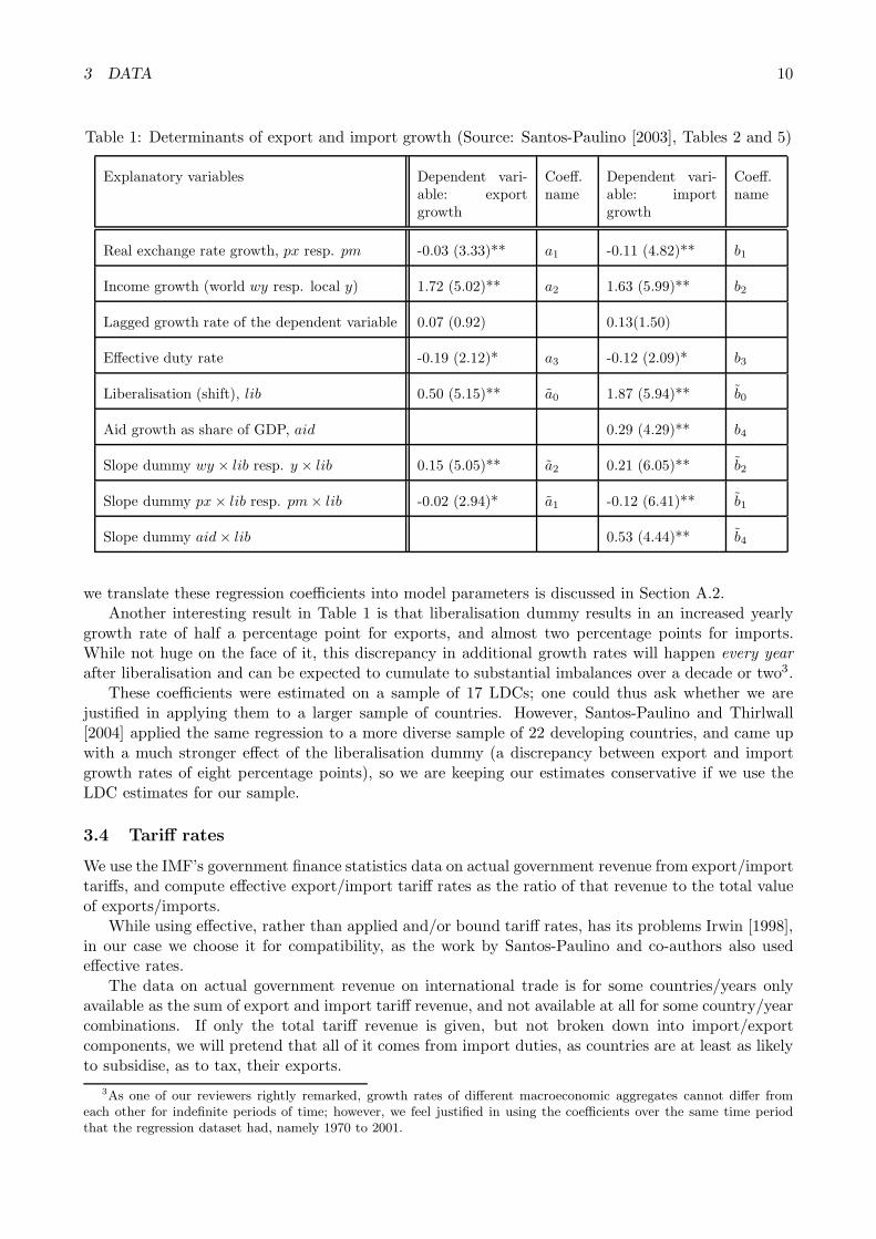
Among the results of Santos-Paulino [2003] there are regressions of the growth rates of exports andimports on their traditional determinants, namely the real exchange rate, growth in income (worldincome for exports, local income for imports), one-year lags of the dependent variable to test for thespeed of adjustment, the effective rate of duties (on exports and imports, respectively; computed asthe ratio of duties actually collected to actual exports and imports respectively), and the non-tarifftrade liberalisation dummy. We reproduce the results that we will be using in Table 1.

The innovative aspect of these regressions is the use of a dummy variable to proxy non-tariff tradeliberalisation. For a given country, that dummy variable is zero until a certain year, ‘initial year oftrade liberalisation’ for that country, and one after that. Despite the simplicity of that representation,Table 1 shows that trade liberalisation thus measured is statistically significant both by itself and ininteraction with the other independent variables. Thus for example, the liberalisation (shift) coefficientfor exports (a0) being equal to 0.5 shows that trade liberalisation increases the growth rate of exportsby half a percentage point.

Let us briefly examine the coefficients in Table 1. Firstly, the lagged growth rate of the dependentvariable is not significant for either exports or imports. This means that long-run elasticities are notsignificantly different from the respective short-run elasticities (at least to the extent that they canbe measured by a regression such as this) and that it is reasonable to assume that adjustments takeplace within one year. That supports our using an equilibrium model on a one-year time scale. How

3 DATA 10

Table 1: Determinants of export and import growth (Source: Santos-Paulino [2003], Tables 2 and 5)

Explanatory variables Dependent vari-able: exportgrowth

Coeff.name

Dependent vari-able: importgrowth

Coeff.name

Real exchange rate growth, px resp. pm -0.03 (3.33)** a1 -0.11 (4.82)** b1

Income growth (world wy resp. local y) 1.72 (5.02)** a2 1.63 (5.99)** b2

Lagged growth rate of the dependent variable 0.07 (0.92) 0.13(1.50)

Effective duty rate -0.19 (2.12)* a3 -0.12 (2.09)* b3

Liberalisation (shift), lib 0.50 (5.15)** a0 1.87 (5.94)** b0

Aid growth as share of GDP, aid 0.29 (4.29)** b4

Slope dummy wy × lib resp. y × lib 0.15 (5.05)** a2 0.21 (6.05)** b2

Slope dummy px × lib resp. pm × lib -0.02 (2.94)* a1 -0.12 (6.41)** b1

Slope dummy aid × lib 0.53 (4.44)** b4

we translate these regression coefficients into model parameters is discussed in Section A.2.Another interesting result in Table 1 is that liberalisation dummy results in an increased yearly

growth rate of half a percentage point for exports, and almost two percentage points for imports.While not huge on the face of it, this discrepancy in additional growth rates will happen every yearafter liberalisation and can be expected to cumulate to substantial imbalances over a decade or two3.

These coefficients were estimated on a sample of 17 LDCs; one could thus ask whether we arejustified in applying them to a larger sample of countries. However, Santos-Paulino and Thirlwall[2004] applied the same regression to a more diverse sample of 22 developing countries, and came upwith a much stronger effect of the liberalisation dummy (a discrepancy between export and importgrowth rates of eight percentage points), so we are keeping our estimates conservative if we use theLDC estimates for our sample.

3.4 Tariff rates

We use the IMF’s government finance statistics data on actual government revenue from export/importtariffs, and compute effective export/import tariff rates as the ratio of that revenue to the total valueof exports/imports.

While using effective, rather than applied and/or bound tariff rates, has its problems Irwin [1998],in our case we choose it for compatibility, as the work by Santos-Paulino and co-authors also usedeffective rates.

The data on actual government revenue on international trade is for some countries/years onlyavailable as the sum of export and import tariff revenue, and not available at all for some country/yearcombinations. If only the total tariff revenue is given, but not broken down into import/exportcomponents, we will pretend that all of it comes from import duties, as countries are at least as likelyto subsidise, as to tax, their exports.

3As one of our reviewers rightly remarked, growth rates of different macroeconomic aggregates cannot differ fromeach other for indefinite periods of time; however, we feel justified in using the coefficients over the same time periodthat the regression dataset had, namely 1970 to 2001.

3 DATA 11

!

" # !

"#$"!

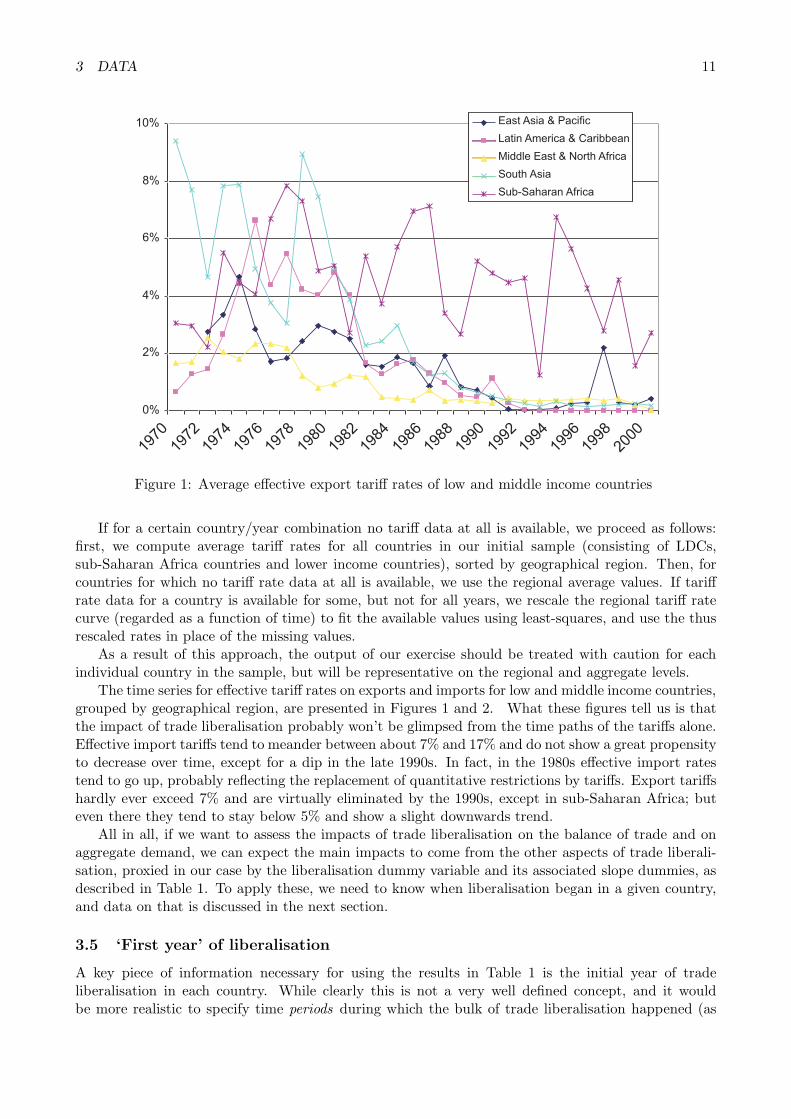
Figure 1: Average effective export tariff rates of low and middle income countries

If for a certain country/year combination no tariff data at all is available, we proceed as follows:first, we compute average tariff rates for all countries in our initial sample (consisting of LDCs,sub-Saharan Africa countries and lower income countries), sorted by geographical region. Then, forcountries for which no tariff rate data at all is available, we use the regional average values. If tariffrate data for a country is available for some, but not for all years, we rescale the regional tariff ratecurve (regarded as a function of time) to fit the available values using least-squares, and use the thusrescaled rates in place of the missing values.

As a result of this approach, the output of our exercise should be treated with caution for eachindividual country in the sample, but will be representative on the regional and aggregate levels.

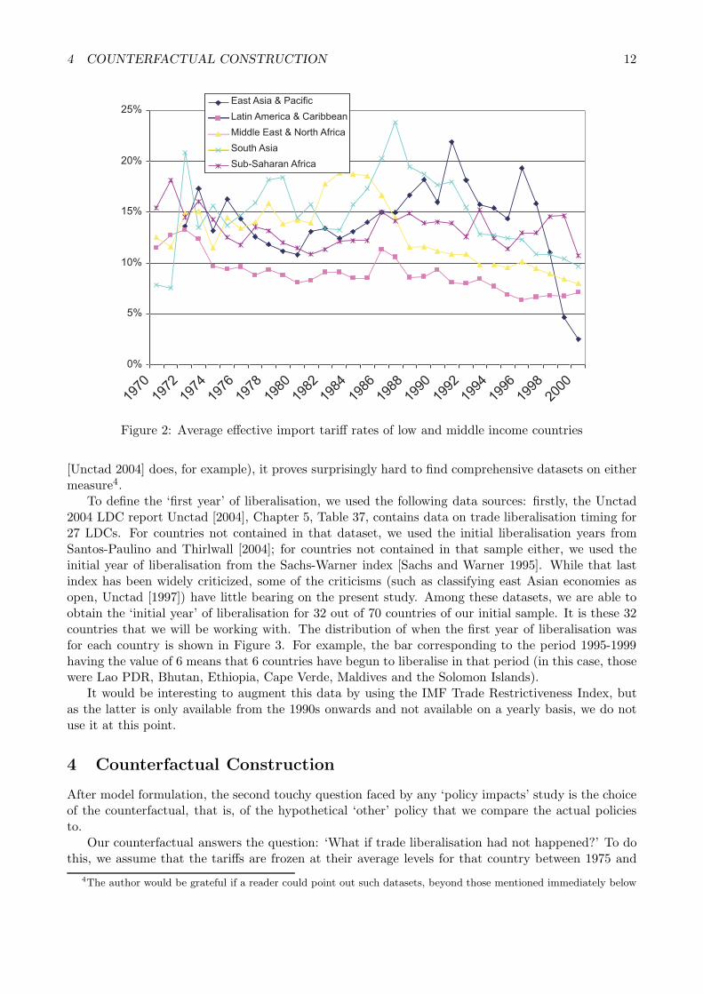
The time series for effective tariff rates on exports and imports for low and middle income countries,grouped by geographical region, are presented in Figures 1 and 2. What these figures tell us is thatthe impact of trade liberalisation probably won’t be glimpsed from the time paths of the tariffs alone.Effective import tariffs tend to meander between about 7% and 17% and do not show a great propensityto decrease over time, except for a dip in the late 1990s. In fact, in the 1980s effective import ratestend to go up, probably reflecting the replacement of quantitative restrictions by tariffs. Export tariffshardly ever exceed 7% and are virtually eliminated by the 1990s, except in sub-Saharan Africa; buteven there they tend to stay below 5% and show a slight downwards trend.

All in all, if we want to assess the impacts of trade liberalisation on the balance of trade and onaggregate demand, we can expect the main impacts to come from the other aspects of trade liberali-sation, proxied in our case by the liberalisation dummy variable and its associated slope dummies, asdescribed in Table 1. To apply these, we need to know when liberalisation began in a given country,and data on that is discussed in the next section.

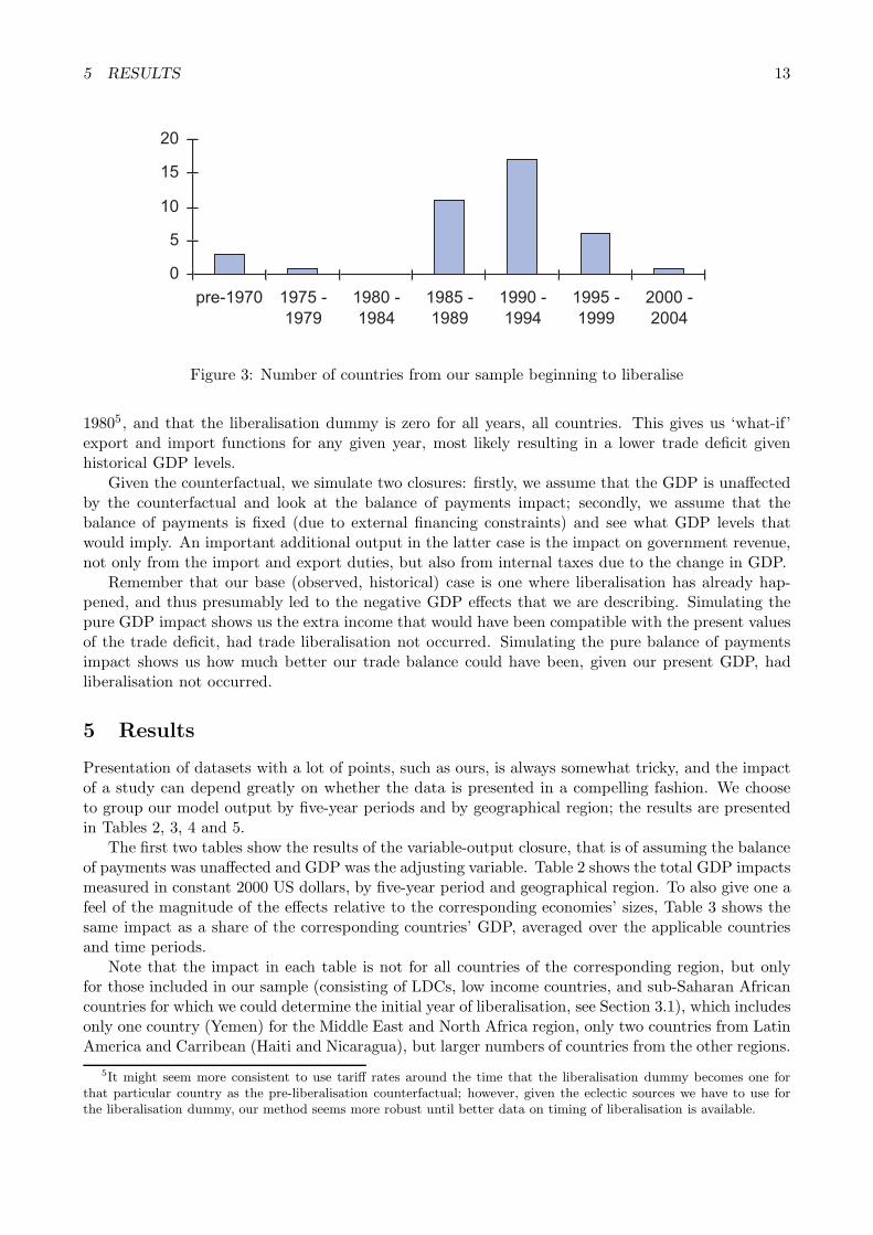
3.5 ‘First year’ of liberalisation

A key piece of information necessary for using the results in Table 1 is the initial year of tradeliberalisation in each country. While clearly this is not a very well defined concept, and it wouldbe more realistic to specify time periods during which the bulk of trade liberalisation happened (as

4 COUNTERFACTUAL CONSTRUCTION 12

%

%

%

!

" # !

"#$"!

Figure 2: Average effective import tariff rates of low and middle income countries

[Unctad 2004] does, for example), it proves surprisingly hard to find comprehensive datasets on eithermeasure4.

To define the ‘first year’ of liberalisation, we used the following data sources: firstly, the Unctad2004 LDC report Unctad [2004], Chapter 5, Table 37, contains data on trade liberalisation timing for27 LDCs. For countries not contained in that dataset, we used the initial liberalisation years fromSantos-Paulino and Thirlwall [2004]; for countries not contained in that sample either, we used theinitial year of liberalisation from the Sachs-Warner index [Sachs and Warner 1995]. While that lastindex has been widely criticized, some of the criticisms (such as classifying east Asian economies asopen, Unctad [1997]) have little bearing on the present study. Among these datasets, we are able toobtain the ‘initial year’ of liberalisation for 32 out of 70 countries of our initial sample. It is these 32countries that we will be working with. The distribution of when the first year of liberalisation wasfor each country is shown in Figure 3. For example, the bar corresponding to the period 1995-1999having the value of 6 means that 6 countries have begun to liberalise in that period (in this case, thosewere Lao PDR, Bhutan, Ethiopia, Cape Verde, Maldives and the Solomon Islands).

It would be interesting to augment this data by using the IMF Trade Restrictiveness Index, butas the latter is only available from the 1990s onwards and not available on a yearly basis, we do notuse it at this point.

4 Counterfactual Construction

After model formulation, the second touchy question faced by any ‘policy impacts’ study is the choiceof the counterfactual, that is, of the hypothetical ‘other’ policy that we compare the actual policiesto.

Our counterfactual answers the question: ‘What if trade liberalisation had not happened?’ To dothis, we assume that the tariffs are frozen at their average levels for that country between 1975 and

4The author would be grateful if a reader could point out such datasets, beyond those mentioned immediately below

5 RESULTS 13

%

%

&$ %$

$

%$

$

%$

$

Figure 3: Number of countries from our sample beginning to liberalise

19805, and that the liberalisation dummy is zero for all years, all countries. This gives us ‘what-if’export and import functions for any given year, most likely resulting in a lower trade deficit givenhistorical GDP levels.

Given the counterfactual, we simulate two closures: firstly, we assume that the GDP is unaffectedby the counterfactual and look at the balance of payments impact; secondly, we assume that thebalance of payments is fixed (due to external financing constraints) and see what GDP levels thatwould imply. An important additional output in the latter case is the impact on government revenue,not only from the import and export duties, but also from internal taxes due to the change in GDP.

Remember that our base (observed, historical) case is one where liberalisation has already hap-pened, and thus presumably led to the negative GDP effects that we are describing. Simulating thepure GDP impact shows us the extra income that would have been compatible with the present valuesof the trade deficit, had trade liberalisation not occurred. Simulating the pure balance of paymentsimpact shows us how much better our trade balance could have been, given our present GDP, hadliberalisation not occurred.

5 Results

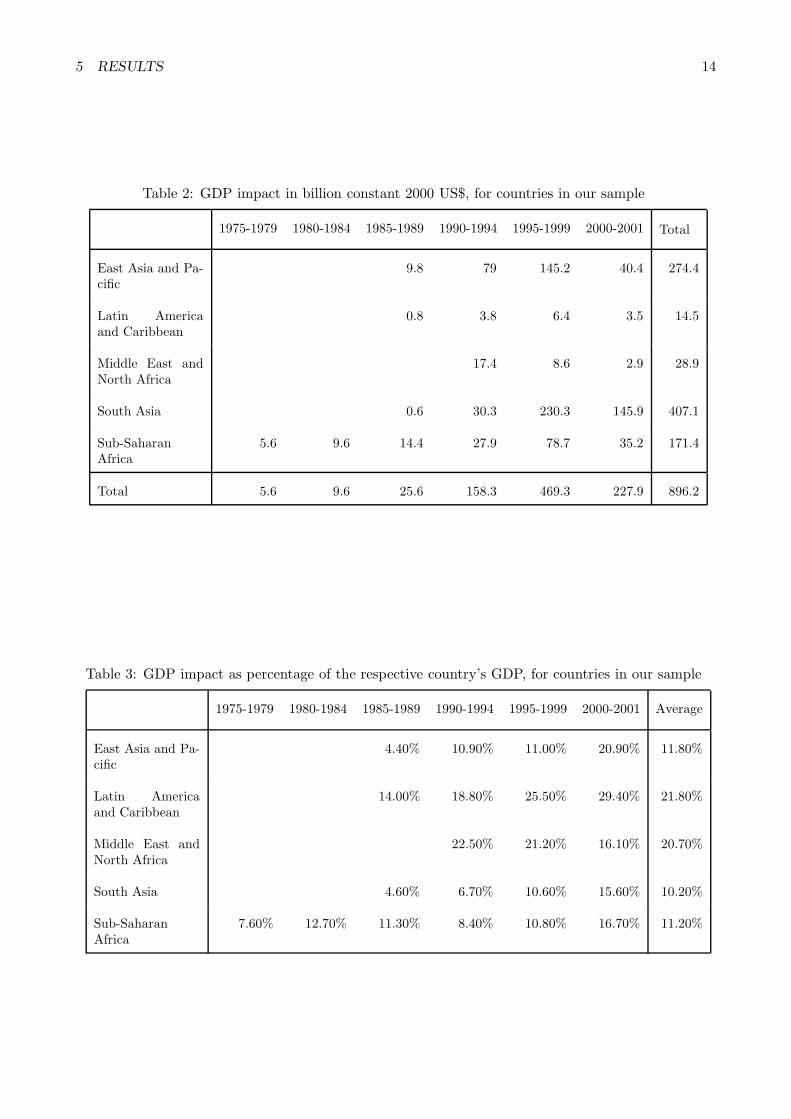
Presentation of datasets with a lot of points, such as ours, is always somewhat tricky, and the impactof a study can depend greatly on whether the data is presented in a compelling fashion. We chooseto group our model output by five-year periods and by geographical region; the results are presentedin Tables 2, 3, 4 and 5.

The first two tables show the results of the variable-output closure, that is of assuming the balanceof payments was unaffected and GDP was the adjusting variable. Table 2 shows the total GDP impactsmeasured in constant 2000 US dollars, by five-year period and geographical region. To also give one afeel of the magnitude of the effects relative to the corresponding economies’ sizes, Table 3 shows thesame impact as a share of the corresponding countries’ GDP, averaged over the applicable countriesand time periods.

Note that the impact in each table is not for all countries of the corresponding region, but onlyfor those included in our sample (consisting of LDCs, low income countries, and sub-Saharan Africancountries for which we could determine the initial year of liberalisation, see Section 3.1), which includesonly one country (Yemen) for the Middle East and North Africa region, only two countries from LatinAmerica and Carribean (Haiti and Nicaragua), but larger numbers of countries from the other regions.

5It might seem more consistent to use tariff rates around the time that the liberalisation dummy becomes one forthat particular country as the pre-liberalisation counterfactual; however, given the eclectic sources we have to use forthe liberalisation dummy, our method seems more robust until better data on timing of liberalisation is available.

5 RESULTS 14

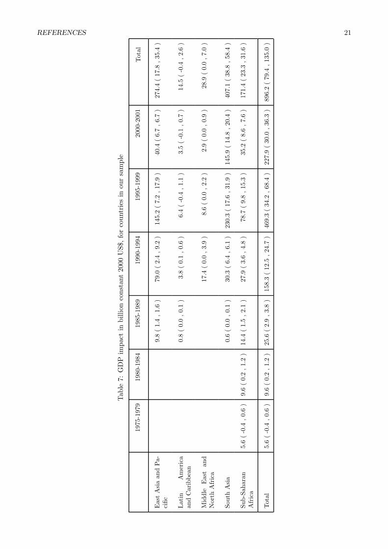
Table 2: GDP impact in billion constant 2000 US$, for countries in our sample

1975-1979 1980-1984 1985-1989 1990-1994 1995-1999 2000-2001 Total

East Asia and Pa-cific

9.8 79 145.2 40.4 274.4

Latin Americaand Caribbean

0.8 3.8 6.4 3.5 14.5

Middle East andNorth Africa

17.4 8.6 2.9 28.9

South Asia 0.6 30.3 230.3 145.9 407.1

Sub-SaharanAfrica

5.6 9.6 14.4 27.9 78.7 35.2 171.4

Total 5.6 9.6 25.6 158.3 469.3 227.9 896.2

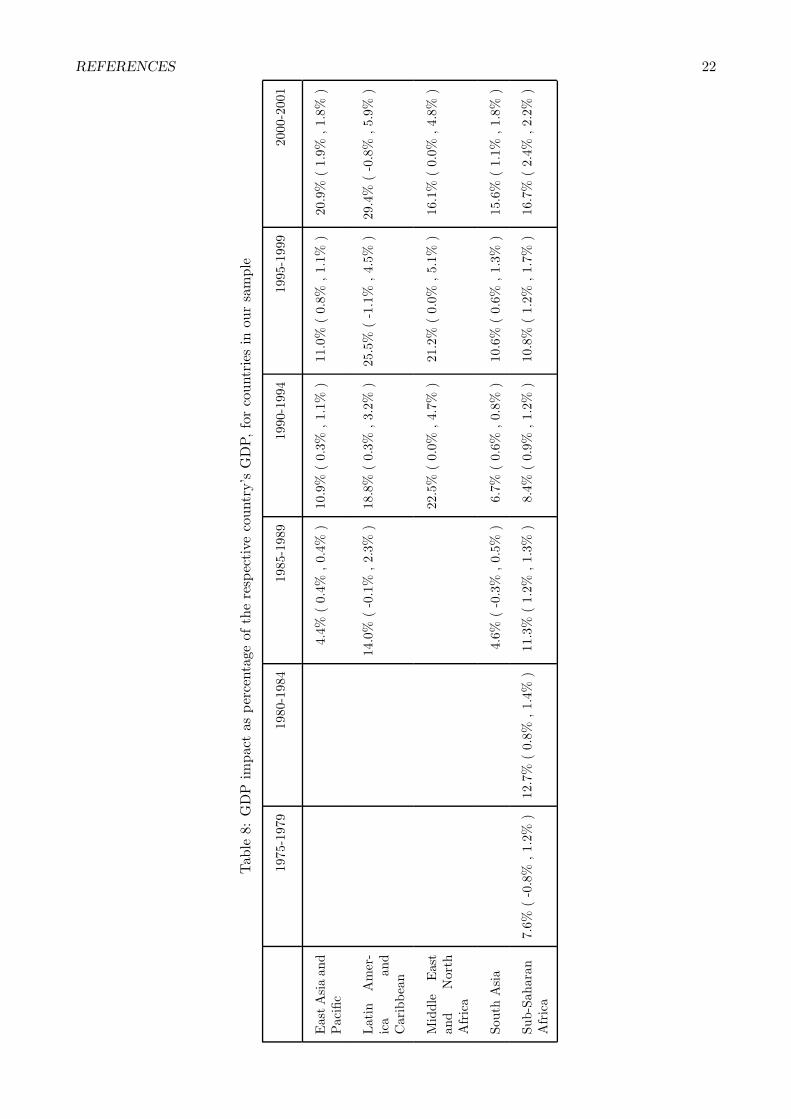
Table 3: GDP impact as percentage of the respective country’s GDP, for countries in our sample

1975-1979 1980-1984 1985-1989 1990-1994 1995-1999 2000-2001 Average


4.40% 10.90% 11.00% 20.90% 11.80%


14.00% 18.80% 25.50% 29.40% 21.80%


22.50% 21.20% 16.10% 20.70%

South Asia 4.60% 6.70% 10.60% 15.60% 10.20%

Sub-SaharanAfrica

7.60% 12.70% 11.30% 8.40% 10.80% 16.70% 11.20%

5 RESULTS 15

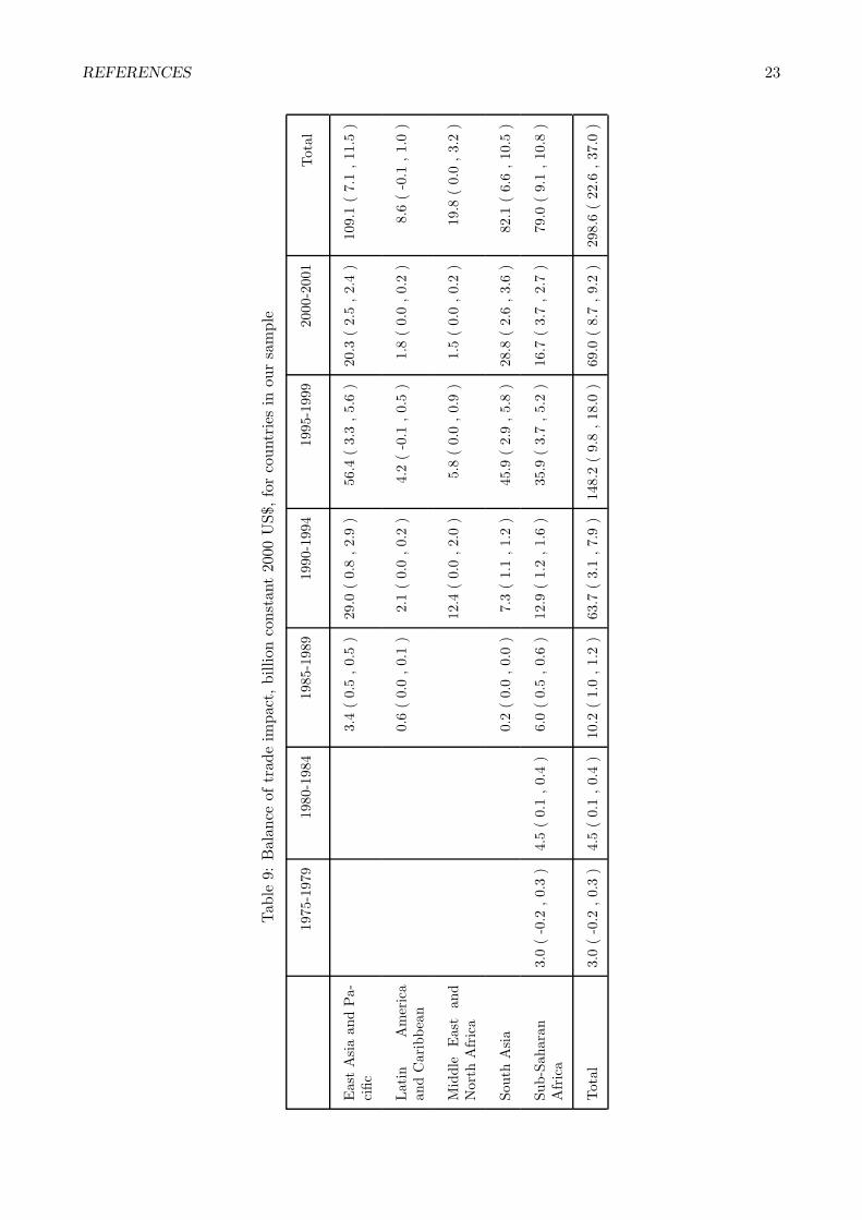
Table 4: Balance of trade impact, billion constant 2000 US$, for countries in our sample

1975-1979 1980-1984 1985-1989 1990-1994 1995-1999 2000-2001 Total


3.4 29 56.4 20.3 109.1


0.6 2.1 4.2 1.8 8.6


12.4 5.8 1.5 19.8

South Asia 0.2 7.3 45.9 28.8 82.1

Sub-SaharanAfrica

3 4.5 6 12.9 35.9 16.7 79

Total 3 4.5 10.2 63.7 148.2 69 298.6

The GDP impacts in constant dollars are increasing from one period to the next (apart from thelast period, which embraces only two years instead of five)6. This follows from the regression results weare using, as once a country has liberalised, the gap between export growth and import growth keepswidening, thus impacts will likely grow over time for any given country. Additionally, as time goesby, more countries are liberalising and contributing to the total. In more open and smaller economies,the trade deficit caused by trade liberalisation will be larger as a share of GDP, and consequently theGDP effects will be more pronounced.

The average impacts as percentage of GDP table do not show the same monotone increase, as fornewly liberalised countries the impacts will be comparatively low as share of GDP, and thus will dragdown the average. For example, this shows in sub-Saharan Africa, where the impacts as percentageof GDP are smaller in 1985-1989 and 1990-1994 than in 1980-1984 due to a large number of newliberalisers in the former two periods.

Overall, we see GDP impacts typically ranging between 10% and 16%, but going as high as 29%in some cases. This loss of aggregate demand towards imports is important both in terms of povertyalleviation and GDP growth potential, since the sectors that are most affected by aggregate demanddeficiency are manufacturing and services – the former being a potential high-value-added sector, andthe latter often containing a large portion of the poor. This broad picture is corroborated by Taylor[2001], a collection of case studies of liberalisation that show the overall impacts on both growth andequity to be neutral to negative7.

Tables 4 and 5 show the corresponding information for the pure balance of payments impact, thatis for assuming the GDP is unaffected and the balance of trade would absorb all the impact. Theoverall picture is comparable to that for GDP impacts, but generally the balance of payments impactsare smaller as the GDP impacts are additionally amplified by multiplier effects. The ratio of balanceof payments to GDP impacts varies, depending on the degree of trade openness of the respectivecountries.

6The exception is Yemen, for which the historical share of imports of GDP has decreased over time, leading todiminished impacts in the counterfactual

7Most countries in these case studies were not part of the sample we consider here, but the trade balance and aggregatedemand effects we focus on played an important role in the case studies.

6 CONCLUSION 16

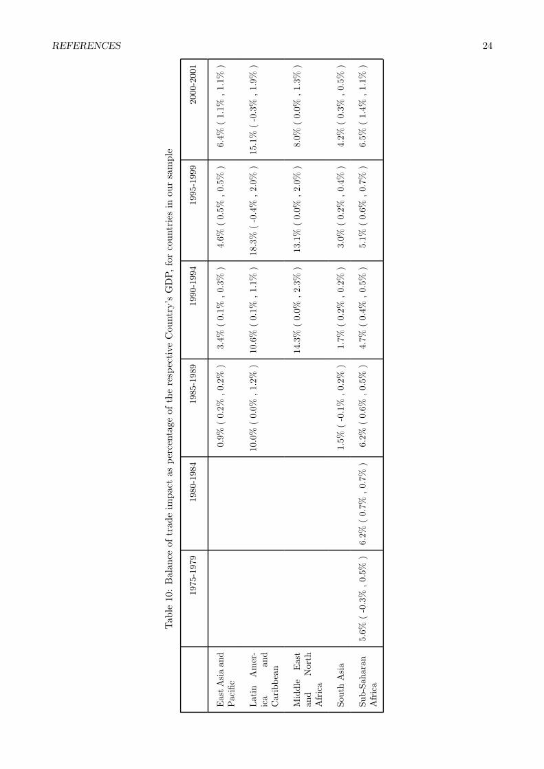
Table 5: Balance of payments impact as percentage of the respective country’s GDP, for countries inour sample

1975-1979 1980-1984 1985-1989 1990-1994 1995-1999 2000-2001 Average


0.90% 3.40% 4.60% 6.40% 4.20%


10.00% 10.60% 18.30% 15.10% 13.90%


14.30% 13.10% 8.00% 12.60%

South Asia 1.50% 1.70% 3.00% 4.20% 2.80%

Sub-SaharanAfrica

5.60% 6.20% 6.20% 4.70% 5.10% 6.50% 5.40%

6 Conclusion

In this paper, we have used regressions by Santos-Paulino [2003], as cited in Unctad [2004], on de-terminants of export and import growth to provide estimates of the impact of trade liberalisation.Our interest was in the foregone opportunities for aggregate demand stimulation or balance of tradeimprovement in the past decades (remember that the balance of payments impact and the privatedisposable income impact are the outcome of two complementary closures, so that the real-life impactwould be a combination of the two).

We have seen that as the increase in import demand due to trade liberalisation outpaced thegrowth in exports, trade liberalisation has likely resulted in additional balance of payments deficitsbetween 2% and 18% of GDP (assuming GDP unaffected), or conversely, in between 4% and 29%aggregate demand loss (assuming balance of payments unaffected). Converting to constant 2000 USdollars, this sums up to 299 · 109 US$ of balance of payments losses, resp. 896 · 109 US$ of aggregatedemand losses.

This loss of aggregate demand towards imports is important both in terms of poverty alleviationand GDP growth potential, since the sectors that are most affected by aggregate demand deficiencyare manufacturing and services – the former being a potential high-value-added sector, and the latteroften containing a large portion of the poor.

A The Model Equations

A.1 The accounting framework

We set up a very simple accounting framework to keep track of economy-wide impacts of changesin the balance of payments. Along with some behavioural assumptions, that gives us a minimalistquantity-clearing CGE model that we will be solving for every country for every year. In fact, thismodel can be regarded as the demand-driven counterpart of the neoclassical 123 model Devarajanet al. [1993] widely promoted by the World Bank8.

8It might appear that our formulation, in contrast to 123, is lacking a role for money supply and the exchangerate. However, this is merely because we are using an abbreviated form where all accounting is done in dollars. It isstraightforward to extend this model to include domestic prices and the money supply with a standard Y = MV kindof equation; however, money supply changes and their impact are not at the center of our present inquiry.

A THE MODEL EQUATIONS 17

The first accounting constraint is the equilibrium in the goods market in volume terms. It can bewritten out as

x + g + c + i = m + y = m + x + nt (1)

Here x, g, c, and i denote the sinks for goods, namely exports, government demand, consumption,and investment demand respectively. y is the real GDP, m are imports, and nt are nontraded goods,all in volume terms. In addition to that, a number of identities in nominal terms need to be satisfied.

First of all, let us have a look at the prices involved. We do all accounting in dollar terms tosimplify the notation. For each volume term v, there are two deflators, the market price Pv and theproducer price Pv, differing because of taxes paid on that term. Since it is precisely the different taxrates that concern us here, we need to write that out carefully. The basic three deflators are pricesfor exports, imports, and nontraded goods. We suppose that duties are paid on exports and imports,and all other government revenue derives from a flat-rate income tax. Then the market prices and theproducer prices are connected through

Pnt = Pnt (2)Pm = Pm (1 + tm) (3)

Px (1 − tx) = Px (4)

Since we can choose the base deflators arbitrarily, we normalize

Px = Pm = 1 (5)

so that (2)-(4) can be rewritten as

Pm = (1 + tm) (6)(1 − tx) = Px (7)

Since we are doing our accounting in dollars, the only prices among those we have just discussed thatwould be affected by changes in real exchange rate are Pnt and Pnt. If we denote the real exchangerate by ε (larger ε corresponds to a real depreciation of the domestic currency), then the equations forPnt and Pnt become

Pnt = Pnt =1ε

(8)

The remaining interesting deflator is the absorption deflator,

Pabs =ntPnt + mPm

nt + m=

nt/ε + m (1 + tm)nt + m

(9)

With the deflators taken care of, we can formulate the accounting framework we use in Table 6.The total tax revenue is likewise just a matter of accounting and is given by

T = xtx + mtm + (x(1 − tx) + nt) tY (10)

A.2 Behavioural equations and closure

The model is completed by specifying the behavioural equations for exports and imports. The sourcefor the specifications is Table 1. However, the regressions presented therein deal with growth rates ofexports and imports, which we need to translate to functions giving the values of exports and importsfor a given year, given their arguments. The somewhat tricky bit are the parts of the functional formthat depend on the liberalisation dummy, as their effects on the growth rate of exports or importscumulate from the beginning of liberalisation onwards.

Let us illustrate the maths on a simple example. Suppose the first year of liberalisation is year 1,and xt is the natural log of exports. For simplicity let’s pretend that xt depends on just one variable

A THE MODEL EQUATIONS 18

Products Private Government Rest of the world

Products C +I = Y −∆Ω G = T − ∆D X = X(. . .)

Private Y = (x(1 − tx) + nt) (1 − tY )

GovernmentT = xtx + mtm+

+ (x(1 − tx) + nt) tY

Rest of theworld

M = M(. . .)

Net savingflows

∆Ω ∆D ∆F

Table 6: The mini-SAM of our model

wyt, but the coefficient consists of a regular part a2 and a liberalisation slope dummy a2. Further,let’s suppose the coefficient of the dummy variable is a0 (tilde denotes “something to do with theliberalisation dummy).

Let us denote with xt the export supply function as it develops under historical conditions (withliberalisation). The equations for the historical growth rate of exports under would then be

x1 − x0 = a0 + (a2 + a2)(wy1 − wy0) (11)x2 − x1 = a0 + (a2 + a2)(wy2 − wy1) (12)

Adding these up yieldsx2 − x0 = 2a0 + (a2 + a2)(wy2 − wy0) (13)

and more generallyxn − x0 = na0 + (a2 + a2)(wyn − wy0) (14)

Now let us consider the export function xn as it would have developed without liberalisation, i.e. withliberalisation dummy off. An argument similar to the above shows

xn − x0 = a2(wyn − wy0). (15)

Subtracting (14) from (15), we obtain

xn = xn + a2(wyn − wyn) − na0 + a2(wy0 − wyn) (16)

Thus, in log terms, the counterfactual export function is the historical exports value, modifiedby the difference between the historical and counterfactual values of the independent variable timesthe no-liberalisation coefficient (second term), plus two additional terms. These two additional termsrepresent the cumulative impact of the liberalisation dummy, through both the shift and the slopedummies. For example, if liberalisation increases the growth rate of exports by 0.5%, then three yearslater, the export function will be 1.5% larger, ceteris paribus; and the extra impacts of the independentvariables that are due to the liberalisation dummy, cumulate in the same way.

The effects of more than one independent variable are added in the same way. Thus in a givenyear, in log terms, the complete equation for export supply is

x = x+a1(RER− RER)+a2(wy− wy)+a3(tx − tx)−na0 + a1(RER0 − RER)+ a2(wy0 − wy) (17)

B SENSITIVITY OF OUR RESULTS TO CHANGES IN REAL EXCHANGE RATE 19

Here the subscript 0 refers to the last year before liberalisation began (in a particular country). Sincewe assume that the world income is not affected by our counterfactual, (17) reduces to

x = x + a1(RER − RER) + a3(tx − tx) − na0 + a1(RER0 − RER) + a2(wy0 − wy). (18)

Converting back from log terms, we get

x = x · exp(a3[tx − tx] − na0

) · (RER

RER

)a1

·(

wy0

wy

)a2

·(

RER0

RER

)a1

. (19)

Similarly, for imports we have

m = m · exp(b3[tx − tx] − nb0

)·(

y

y

)b2

·(

RER

RER

)b1

·(

y0

y

)b2

·(

RER0

RER

)b1

·(

aid0

aid

)b2

. (20)

The main closure we are using is balance of payments-constrained variable output. To be precise,we assume that the internal and external financing possibilities are constrained, so that when lowertariffs worsen both the balance of payments and the government deficit, both the external inflows∆F and the domestic government borrowing ∆D stay constant. By the law of Walras, that meansthat the net lending of the private sector ∆Ω will also remain constant. Then government demandmust necessarily be given by G = T − ∆D and total private demand by C + I = Y − ∆Ω. In thissetting, domestic nontraded output is the equilibrating variable. An alternative we also consider isthe ‘balance of payments’ closure, with the balance of payments being the equilibrating variable. Themeaning of and justifications for both closures are discussed in the body of the paper.

B Sensitivity of our results to changes in real exchange rate

An important relationship that our model, as presented so far, had to leave unexplored, was theinfluence of trade liberalisation-induced changes in the real exchange rate on our results. The causefor that omission was the lack of a usable theory of real exchange rate behavior, as discussed inSection 2.4.6.

As a first step towards estimating the importance of the issue, the maximal magnitude of theexpected impact of accounting for exchange rate depreciation can already be seen from a back-of-theenvelope computation, as follows: suppose as an extreme case, that all of the real exchange rate(RER) changes occurring during or close to trade liberalisation episodes are actually due to tradeliberalisation. If we look at the data on 13 liberalising LDCs in Tables 38 and 39 of [Unctad 2004,p.187], we see that trade liberalisation has been accompanied on average by a RER depreciationof 35% happening over an average period of about 12 years. That gives us an average rate of RERdepreciation of about three percentage points per year associated with trade liberalisation. Combiningthis with the total RER elasticity of imports of 0.11 (b1 in Table 1, Section 3.3, compare Equation (19)) gives us a yearly increase in import demand of about 0.33 percentage points (according to Table 1,impact of RER on exports is negligible). This reduces the post-liberalisation import growth increase,ceteris paribus, from 1.87 to 1.53 percentage points, and the gap between exports and imports growthrates (the variable that drives the increase in trade deficit) from 1.37 to 1.04 percentage points. Thisleads us to conclude that even if we attribute all of the observed exchange rate depreciation to tradeliberalisation (that is, we assume it would not have happened, had trade liberalisation not taken place),that would decrease the size of our main effect by less than a quarter (and even less if historical valueof imports in the year in question exceeds that of exports).

The exchange rate depreciation effect would cease after those initial 12 years, but as Figure 3shows, most of the countries in the sample have liberalised since the late 1980s, so this is just aboutthe time frame that our simulations extend over.

Now to the actual simulations. The equations we have derived, such as (8), (19), and (20) didinclude the real exchange rate, and the purpose of the present appendix is to test the sensitivity of the

REFERENCES 20

model output to two counterfactual scenarios of exchange rate behaviour. The first RER counterfactualis restoring the real exchange rate to its value in the last year before liberalisation began; the secondRER counterfactual is assuming a yearly 3% real depreciation starting in the initial liberalisation year– this is an average observed rate derived from Unctad [2004], as discussed in Section 2.4.6. Sincetypically a real depreciation will decrease imports, it will reduce the GDP and balance of paymentsimpacts that we estimate here; the only question is by how much. In order to indicate this, wereproduce the tables from the Results section, but now with each number followed by the differencebetween the base run and the two counterfactuals. Thus, 10(1, 3) would mean that the base run valuewas 10, the first counterfactual was 9, and the second counterfactual was 7.

Looking at these simulations, we see two things: firstly, the impact of the second RER counterfac-tual (assuming yearly 3% RER depreciation) is virtually always stronger than of the first (restoringRER to its last pre-liberalisation value), so the 3% value was a reasonable one to choose. Secondly,the overall sensitivity to changing the RER is rarely above a quarter of the underlying number, and inmost cases is less than a tenth thereof. Thus, while not insignificant, not dealing with RER impactsin the body of the paper was not a crippling problem.

References

K J Arrow. ‘General Economic Equilibrium: Purpose, analytic techniques, collective choice.’ TheAmerican Economic Review, 64(3):253–272, June 1974.

J Berg and L Taylor. External Liberalisation, Economic Performance and Social Policy, volume 12 ofCEPA Working Paper Series I. Center for Economic Policy Analysis, February 2000.

L de Maio, F Stewart, and R van der Hoeven. Computable general equilibrium models, adjustment,and the poor in Africa. World Development, 27(3):453–470, 1999.

S Devarajan, J Lewis, and S Robinson. ‘External shocks, purchasing power parity and the equilibriumreal exchange rate.’ The World Bank Economic Review, 7:45–63, 1993.

S Devarajan and J D Lewis. ‘Policy lessons from trade-focused, two-sector models.’ Journal of PolicyModeling, 12:625–657, 1990.

W Godley and F Cripps. Macroeconomics. Fontana Paperbacks, 1983.

D Irwin. ‘Changes in U.S. tariffs: The role of import prices and commercial policies.’ AmericanEconomic Review, pages 1015–26, September 1998.

E Kraev. Modeling Macroeconomic and Distributional Impacts of Stabilization and Adjustment Pack-ages: Current Literature and Challenges. CEPA Working Papers. Center for Economic PolicyAnalysis, New School for Social Research, New York, 2003.

J Sachs and A Warner. Economic reform and the process of global integration. Brookings Papers onEconomic Activity. The Brookings Institution, 1995.

D E Sahn, P A Dorosh, and S D Younger. Exchange rate, fiscal and agricultural policies in Africa:Does adjustment hurt the poor? World Development, 24(4):719–747, 1996.

A U Santos-Paulino. The effect of trade liberalisation on import growth in developing countries. WorldDevelopment, 30:959–974, 2002a.

A U Santos-Paulino. Trade liberalisation and export performance in selected developing countries.Journal of Development Studies, 39:140–164, 2002b.

REFERENCES 21

Tab

le7:

GD

Pim

pact

inbi

llion

cons

tant

2000

US$

,fo

rco

untr

ies

inou

rsa

mpl

e

1975

-197

919

80-1

984

1985

-198

919

90-1

994

1995

-199

920

00-2

001

Tot

al

Eas

tA

sia

and

Pa-

cific

9.8

(1.

4,1.

6)

79.0

(2.

4,9.

2)

145.

2(

7.2

,17.

9)

40.4

(6.

7,6.

7)

274.

4(

17.8

,35

.4)

Lat

inA

mer

ica

and

Car

ibbe

an0.

8(

0.0

,0.

1)

3.8

(0.

1,0.

6)

6.4

(-0

.4,1.

1)

3.5

(-0

.1,0.

7)

14.5

(-0

.4,2.

6)

Mid

dle

Eas

tan

dN

orth

Afr

ica

17.4

(0.

0,3.

9)

8.6

(0.

0,2.

2)

2.9

(0.

0,0.

9)

28.9

(0.

0,7.

0)

Sout

hA

sia

0.6

(0.

0,0.

1)

30.3

(6.

4,6.

1)

230.

3(

17.6

,31.

9)

145.

9(

14.8

,20

.4)

407.

1(

38.8

,58

.4)

Sub-

Saha

ran

Afr

ica

5.6

(-0

.4,0.

6)

9.6

(0.

2,1.

2)

14.4

(1.

5,2.

1)

27.9

(3.

6,4.

8)

78.7

(9.

8,1

5.3

)35

.2(

8.6

,7.

6)

171.

4(

23.3

,31

.6)

Tot

al5.

6(

-0.4

,0.

6)

9.6

(0.

2,1.

2)

25.6

(2.

9,3.

8)

158.

3(

12.5

,24.

7)

469.

3(

34.2

,68.

4)

227.

9(

30.0

,36

.3)

896.

2(

79.4

,13

5.0

)

REFERENCES 22

Tab

le8:

GD

Pim

pact

aspe

rcen

tage

ofth

ere

spec

tive

coun

try’

sG

DP,

for

coun

trie

sin

our

sam

ple

1975

-197

919

80-1

984

1985

-198

919

90-1

994

1995

-199

920

00-2

001

Eas

tA

sia

and

Pac

ific

4.4%

(0.

4%,0.

4%)

10.9

%(

0.3%

,1.

1%)

11.0

%(

0.8%

,1.

1%)

20.9

%(

1.9%

,1.8

%)

Lat

inA

mer

-ic

aan

dC

arib

bean

14.0

%(

-0.1

%,2.

3%)

18.8

%(

0.3%

,3.

2%)

25.5

%(

-1.1

%,4.

5%)

29.4

%(

-0.8

%,5

.9%

)

Mid

dle

Eas

tan

dN

orth

Afr

ica

22.5

%(

0.0%

,4.

7%)

21.2

%(

0.0%

,5.

1%)

16.1

%(

0.0%

,4.8

%)

Sout

hA

sia

4.6%

(-0

.3%

,0.

5%)

6.7%

(0.

6%,0.

8%)

10.6

%(

0.6%

,1.

3%)

15.6

%(

1.1%

,1.8

%)

Sub-

Saha

ran

Afr

ica

7.6%

(-0

.8%

,1.

2%)

12.7

%(

0.8%

,1.

4%)

11.3

%(

1.2%

,1.

3%)

8.4%

(0.

9%,1.

2%)

10.8

%(

1.2%

,1.

7%)

16.7

%(

2.4%

,2.2

%)

REFERENCES 23

Tab

le9:

Bal

ance

oftr

ade

impa

ct,bi

llion

cons

tant

2000

US$

,fo

rco

untr

ies

inou

rsa

mpl

e

1975

-197

919

80-1

984

1985

-198

919

90-1

994

1995

-199

920

00-2

001

Tot

al

Eas

tA

sia

and

Pa-

cific

3.4

(0.

5,0.

5)

29.0

(0.

8,2

.9)

56.4

(3.

3,5.

6)

20.3

(2.

5,2.

4)

109.

1(

7.1

,11

.5)

Lat

inA

mer

ica

and

Car

ibbe

an0.

6(

0.0

,0.

1)

2.1

(0.

0,0

.2)

4.2

(-0

.1,0.

5)

1.8

(0.

0,0.

2)

8.6

(-0

.1,1.

0)

Mid

dle

Eas

tan

dN

orth

Afr

ica

12.4

(0.

0,2

.0)

5.8

(0.

0,0.

9)

1.5

(0.

0,0.

2)

19.8

(0.

0,3.

2)

Sout

hA

sia

0.2

(0.

0,0.

0)

7.3

(1.

1,1

.2)

45.9

(2.

9,5.

8)

28.8

(2.

6,3.

6)

82.1

(6.

6,10

.5)

Sub-

Saha

ran

Afr

ica

3.0

(-0

.2,0.

3)

4.5

(0.

1,0.

4)

6.0

(0.

5,0.

6)

12.9

(1.

2,1

.6)

35.9

(3.

7,5.

2)

16.7

(3.

7,2.

7)

79.0

(9.

1,10

.8)

Tot

al3.

0(

-0.2

,0.

3)

4.5

(0.

1,0.

4)

10.2

(1.

0,1.

2)

63.7

(3.

1,7

.9)

148.

2(

9.8

,18.

0)

69.0

(8.

7,9.

2)

298.

6(

22.6

,37

.0)

REFERENCES 24

Tab

le10

:B

alan

ceof

trad

eim

pact

aspe

rcen

tage

ofth

ere

spec

tive

Cou

ntry

’sG

DP,

for

coun

trie

sin

our

sam

ple

1975

-197

919

80-1

984

1985

-198

919

90-1

994

1995

-199

920

00-2

001

Eas

tA

sia

and

Pac

ific

0.9%

(0.

2%,0.

2%)

3.4%

(0.

1%,0.

3%)

4.6%

(0.

5%,0.

5%)

6.4%

(1.

1%,1.

1%)

Lat

inA

mer

-ic

aan

dC

arib

bean

10.0

%(

0.0%

,1.

2%)

10.6

%(

0.1%

,1.

1%)

18.3

%(

-0.4

%,2.

0%)

15.1

%(

-0.3

%,1.

9%)

Mid

dle

Eas

tan

dN

orth

Afr

ica

14.3

%(

0.0%

,2.

3%)

13.1

%(

0.0%

,2.

0%)

8.0%

(0.

0%,1.

3%)

Sout

hA

sia

1.5%

(-0

.1%

,0.

2%)

1.7%

(0.

2%,0.

2%)

3.0%

(0.

2%,0.

4%)

4.2%

(0.

3%,0.

5%)

Sub-

Saha

ran

Afr

ica

5.6%

(-0

.3%

,0.

5%)

6.2%

(0.

7%,0.

7%)

6.2%

(0.

6%,0.

5%)

4.7%

(0.

4%,0.

5%)

5.1%

(0.

6%,0.

7%)

6.5%

(1.

4%,1.

1%)

REFERENCES 25

A U Santos-Paulino. Trade liberalisation, exports, imports, aid, and the balance of payments in leastdeveloped countries. Background paper prepared for the Least Developed Countries Report 2004,Unctad, Geneva, 2003.

A U Santos-Paulino and A P. Thirlwall. The effects of trade liberalisation on imports in selecteddeveloping countries. The Economic Journal, 114, February 2004.

L Taylor. Gap models. Journal of Development Economics, 45:17–34, 1994.

L Taylor, editor. External Liberalisation, Economic Performance, and Social Policy. Oxford UniversityPress, 2001.

L Taylor. Reconstructing Macroeconomics : Structuralist Proposals and Critiques of the Mainstream.Harvard University Press, 2004.

Unctad. Unctad Trade and Development Report 1997. United Nations publication, 1997.

Unctad. The Least Developed Countries Report 2004. United Nations publication, 2004.

Estimating GDP effects of trade liberalisation on ...

Documents

Transcript of Estimating GDP effects of trade liberalisation on ...