Essays in Telecommunications Policy and Management

Submitted in partial fulfillment of the requirements for

the degree of

Doctor of Philosophy

in

Engineering and Public Policy

Miguel Godinho de Matos

B.S., Computer Science and Engineering, IST - Technical University of LisbonM.S., Computer Science and Engineering, IST - Technical University of Lisbon

M.S., Engineering and Public Policy, Carnegie Mellon University

Carnegie Mellon UniversityPittsburgh, PA

August 2013

For my wife, my son and for my parents

iv

AbstractThis work comprises three independent essays in Telecommunications Policy

and Management.In the first study we focus on the deployment of green field next generation

access network infrastructures when the national regulatory authority has thepower to define geographical markets at sub-national level for which it can ap-ply differentiated regulatory remedies - Geographically Segmented Regulation(GSR). Using a game theory model that we developed, we confirm the asymmet-ric business case for the geographic development of these new infrastructures:highly populated areas are likely to develop into competitive telecommunicationmarkets while regions with low household density will only see limited invest-ment and little or no competition. We show that supply side interdependenciesamong markets make the implementation of GSR non-trivial, namely, we showthat changes in the wholesale access price in one market can have undesir-able consequences in the competitive conditions of interrelated regions wherewholesale prices are unchanged.

In the second study we focus on how individual purchase decisions are in-fluenced by the behavior of others in their social circle. We study the case ofthe diffusion of the iPhone 3G across a number of communities sampled froma dataset provided by a major mobile carrier in one country. We find thatthe propensity of adoption increases with the proportion of each indivudal’sadopter friends. We estimate that 14% of iPhone 3G adoptions in this carrierwere due to peer influence. We provide results from several policy experimentsthat show that with this level of effect from peer influence the carrier wouldhardly be able to significantly increase sales by selectively targeting consumersto benefit from viral marketing.

Finally, in the third study, we perform a randomized field experiment todetermine the role that likes play on the sales of movies in Video-on-Demand(VoD). We use the VoD system of a large telecommunications provider duringhalf a year in 2012. The system suggests movies to consumers ordered by thenumber of consumer likes they obtained in previous weeks. We manipulatedsuch natural order by randomly swapping likes across movies. We found thatmovies promoted (demoted) increased (decreased) sales, but the amount of in-formation publicly available about movies affected the result. Better knownmovies were less sensitive to manipulations. Finally a movie promoted (de-moted) to a fake slot sold 15.9% less (27.7% more) than a true movie placed atthat slot, on average across all manipulations. A movie promoted (demoted)to a fake slot received 33.1% fewer (30.1% more) likes than a true movie atthat slot. Hence manipulated movies tended to move back to their true slotsover time. This means that self-fulfilling prophecies widely discussed in theliterature on the effect of ratings on sales are hard to sustain in markets withcostly goods that are sufficiently well-known.

vi

Acknowledgments

I would like to acknowledge the financial support provided by the PortugueseFoundation for Science and Technology through the Carnegie Mellon PortugalProgram under Grant SFRH/BD/33772/2009.

I would also like to acknowledge the two industrial partners that allowed meto use their databases without which this work would not have been possible.

I would like to thank Professor Pedro Ferreira, my advisor, for all his supportand professional as well as personal guidance during this journey. For the livelydiscussions, and for all the time he dedicated to my research.

I would like to extend a special thank you to Professor David Krackhardtand to Professor Rahul Telang who had particularly active roles in the co-supervision of my research and to whom I am indebt for the time, expertise,recommendations and constructive criticism.

Finally, I would also like to thank all members of my Ph.D. committee:Professor Pedro Ferreira (chair), Professor Francisco Lima (co-chair), ProfessorDavid Krackhardt, Professor Rahul Telang, Professor Marvin Sirbu, ProfessorRavi Bapna, and Professor Joao Paulo Costeira for their interest in my research.

viii

Contents

1 Introduction 1References . . . . . . . . . . . . . . . . . . . . . . . . . . . . . . . . . . . . . . . 5

2 Wholesale Price Regulation in Telecoms with Endogenous Entry andSimultaneous Markets 72.1 Introduction . . . . . . . . . . . . . . . . . . . . . . . . . . . . . . . . . . . 82.2 Model Description . . . . . . . . . . . . . . . . . . . . . . . . . . . . . . . 152.3 Model Parameterization . . . . . . . . . . . . . . . . . . . . . . . . . . . . 172.4 Single Market Simulation . . . . . . . . . . . . . . . . . . . . . . . . . . . . 222.5 Multi Market Simulation . . . . . . . . . . . . . . . . . . . . . . . . . . . . 292.6 Conclusions . . . . . . . . . . . . . . . . . . . . . . . . . . . . . . . . . . . 33References . . . . . . . . . . . . . . . . . . . . . . . . . . . . . . . . . . . . . . . 372.A Simulating the linear demand curve . . . . . . . . . . . . . . . . . . . . . . 41

3 Peer Influence in Product Diffusion over Very Large Social Networks 433.1 Introduction . . . . . . . . . . . . . . . . . . . . . . . . . . . . . . . . . . . 443.2 Literature Review . . . . . . . . . . . . . . . . . . . . . . . . . . . . . . . . 50

3.2.1 Diffusion and Peer Influence . . . . . . . . . . . . . . . . . . . . . . 503.2.2 Related Studies . . . . . . . . . . . . . . . . . . . . . . . . . . . . . 52

3.3 The iPhone 3G and the EURMO dataset . . . . . . . . . . . . . . . . . . . 593.3.1 iPhone 3G Release . . . . . . . . . . . . . . . . . . . . . . . . . . . 593.3.2 Raw Dataset . . . . . . . . . . . . . . . . . . . . . . . . . . . . . . 613.3.3 Social Network . . . . . . . . . . . . . . . . . . . . . . . . . . . . . 61

3.4 Community Based Sample . . . . . . . . . . . . . . . . . . . . . . . . . . . 623.4.1 Community Identification Algorithms . . . . . . . . . . . . . . . . . 653.4.2 Community Identification . . . . . . . . . . . . . . . . . . . . . . . 673.4.3 T-CLAP community sample . . . . . . . . . . . . . . . . . . . . . . 68

3.5 Consumer Utility Model . . . . . . . . . . . . . . . . . . . . . . . . . . . . 753.6 Peer Influence Estimate . . . . . . . . . . . . . . . . . . . . . . . . . . . . 833.7 Robustness Checks . . . . . . . . . . . . . . . . . . . . . . . . . . . . . . . 89

3.7.1 Instrument Robustness . . . . . . . . . . . . . . . . . . . . . . . . . 893.7.2 Alternative Weight Matrices . . . . . . . . . . . . . . . . . . . . . . 933.7.3 The impact of having a time varying social network . . . . . . . . . 97

3.8 Policy Experiment . . . . . . . . . . . . . . . . . . . . . . . . . . . . . . . 106

ix

3.9 Conclusion . . . . . . . . . . . . . . . . . . . . . . . . . . . . . . . . . . . . 108References . . . . . . . . . . . . . . . . . . . . . . . . . . . . . . . . . . . . . . . 1153.A Full Regression Results . . . . . . . . . . . . . . . . . . . . . . . . . . . . . 1273.B Instrumental Variable Details . . . . . . . . . . . . . . . . . . . . . . . . . 1303.C Summary of the community identification algorithms . . . . . . . . . . . . 133

3.C.1 The T-CLAP algorithm (Zhang and Krackhardt, 2011) . . . . . . . 1333.C.2 The walktrap algorithm (Pons and Latapy, 2006) . . . . . . . . . . 1343.C.3 Label propagation algorithm (Raghavan et al., 2007) . . . . . . . . 1353.C.4 Fast greedy modularity optimization (Clauset et al., 2004) . . . . . 1353.C.5 The Louvain’s method (Blondel et al., 2008) . . . . . . . . . . . . . 1363.C.6 The infomap algorithm (Rosvall and Bergstrom, 2008) . . . . . . . 137

3.D Further details of the SIENA Analysis . . . . . . . . . . . . . . . . . . . . 1373.D.1 Robustness of the Network− > Behavior effect . . . . . . . . . . . 1373.D.2 Alternative partitions of the time period . . . . . . . . . . . . . . . 138

4 The Impact of Likes on the Sales of Movies in Video-on-Demand: aRandomized Experiment 1454.1 Introduction . . . . . . . . . . . . . . . . . . . . . . . . . . . . . . . . . . . 1464.2 Related Literature . . . . . . . . . . . . . . . . . . . . . . . . . . . . . . . 1504.3 The Context of Our Experiment . . . . . . . . . . . . . . . . . . . . . . . . 155

4.3.1 The Company and its Dataset . . . . . . . . . . . . . . . . . . . . . 1554.3.2 VoD Service and Interface . . . . . . . . . . . . . . . . . . . . . . . 157

4.4 Experimental Design . . . . . . . . . . . . . . . . . . . . . . . . . . . . . . 1604.5 Empirical Model . . . . . . . . . . . . . . . . . . . . . . . . . . . . . . . . 163

4.5.1 Movie Level Specification . . . . . . . . . . . . . . . . . . . . . . . . 1634.5.2 The Magnitude of Treatment . . . . . . . . . . . . . . . . . . . . . 1644.5.3 Identification and Exogeneity . . . . . . . . . . . . . . . . . . . . . 1654.5.4 Rank Level Specification . . . . . . . . . . . . . . . . . . . . . . . . 165

4.6 Results and Discussion . . . . . . . . . . . . . . . . . . . . . . . . . . . . . 1664.6.1 Descriptive Statistics . . . . . . . . . . . . . . . . . . . . . . . . . . 1664.6.2 The Effect of Swaps and the Role of Rank . . . . . . . . . . . . . . 1744.6.3 The Role of Outside Information . . . . . . . . . . . . . . . . . . . 1794.6.4 Converge to True Ranks . . . . . . . . . . . . . . . . . . . . . . . . 180

4.7 Conclusions . . . . . . . . . . . . . . . . . . . . . . . . . . . . . . . . . . . 183References . . . . . . . . . . . . . . . . . . . . . . . . . . . . . . . . . . . . . . . 1874.A High and Low Intensity VoD Users . . . . . . . . . . . . . . . . . . . . . . 1914.B Impact of Rank on Trailer Views . . . . . . . . . . . . . . . . . . . . . . . 1954.C Eliminating Sequences of Treatments . . . . . . . . . . . . . . . . . . . . . 1974.D Berry, Levinsohn, Pakes model (BLP) . . . . . . . . . . . . . . . . . . . . . 199

5 Conclusion 205

x

List of Figures

2.1 1 % of households subscribing to Fiber-to-the-Home/Building in February2010. Graphic taken from(Begonha et al., 2010) . . . . . . . . . . . . . . . 9

2.2 Breakdown of the research efforts according to their main concerns in whatrespects the telecommunications’ industry . . . . . . . . . . . . . . . . . . 10

2.3 Structure of the model . . . . . . . . . . . . . . . . . . . . . . . . . . . . . 19

2.4 Outcome of single market simulations. The first row details the total numberof firms that enter the market and the second row specifies which of these areinfrastructure providers. The bottom row quantifies the consumer surplusin each scenario. All images are built based on a temperature map wherewarmer colors indicate higher values. In rows one and two, the coolest colorcorresponds to combinations of the wholesale price and infrastructure costsfor which there is no pure strategies equilibrium. . . . . . . . . . . . . . . . 28

2.5 Summary output of the simulation. The panels illustrate the equilibriumvalues of the main variables being monitored in each of the two marketsconsidered in this simulation. The simulation considers that 2 RIPs and 1VP consider entry in both markets simultaneously . . . . . . . . . . . . . . 34

2.6 The left panel displays the WTP distribution for a region with 200,000households and the right panel displays the corresponding estimation of thedemand curve . . . . . . . . . . . . . . . . . . . . . . . . . . . . . . . . . . 42

3.1 Most important characteristics considered when purchasing a new handset(% of total respondents who named each particular characteristic) . . . . . 60

3.2 Empirical degree distribution of our communications graph. Grey dots rep-resent subscribers whose out-degree is three standard deviations below themean . . . . . . . . . . . . . . . . . . . . . . . . . . . . . . . . . . . . . . . 63

3.3 Path between subscribers in distinct communities . . . . . . . . . . . . . . 72

3.4 Number of adoptions each month for the subscribers in the sample. The 0in the x-axis indicates the month of July which coincides with the releaseperiod of the iPhone 3G handset . . . . . . . . . . . . . . . . . . . . . . . . 74

3.5 Communities extracted with the modified T-CLAP algorithm . . . . . . . 74

3.6 The role of peer influence in the adoption of the iPhone 3G . . . . . . . . . 88

3.7 Percentage of accounts with less than six members per number of adopters 90

3.8 Scatter plot for the 153 estimates of theNetwork− > Behavior andBehavior− >Network variables of the SIENA model . . . . . . . . . . . . . . . . . . . 104

xi

3.9 Policy outcomes of awarding the iPhone 3G to different numbers of policytargets . . . . . . . . . . . . . . . . . . . . . . . . . . . . . . . . . . . . . . 109

3.10 Potential profits from seeding the iPhone 3G with global degree . . . . . . 1103.11 Number of NUTS-III codes where subscribers received or placed calls from

August 2008 until July 2009 . . . . . . . . . . . . . . . . . . . . . . . . . . 1313.12 Proportion of phone calls within the primary NUTS-III region from August

2008 until July 2009 . . . . . . . . . . . . . . . . . . . . . . . . . . . . . . 1323.13 Meta-analysis sensitivity plots for the meta analysis for the Network− >

Behavior variable of the SIENA model . . . . . . . . . . . . . . . . . . . . 1403.14 Meta-analysis diagnostic plots for the Network− > Behavior variable of

the SIENA model . . . . . . . . . . . . . . . . . . . . . . . . . . . . . . . . 141

4.1 Revenues of movie distributors in the US market as a percentage of GDP(excluding merchandising). Source: (Waterman, 2011) . . . . . . . . . . . . 147

4.2 Summary of the main features available to subscribers of our IP. . . . . . 1574.3 30-Day Moving Average of Daily Leases in Highlights and Catalog in IP’s

VoD. . . . . . . . . . . . . . . . . . . . . . . . . . . . . . . . . . . . . . . . 1684.4 30-Day Moving Average of Daily Leases in Highlights per Menu in IP’s VoD. 1684.5 Sales in the New Menu During Our Experiment. . . . . . . . . . . . . . . . 1694.6 Number of Likes per Rank at the New Menu in the Beginning of the Week. 1704.7 Leases per Week as Function of Rank at the New Menu. . . . . . . . . . . 1714.8 Likes per Week as a Function of Rank for All, Control and Treated Movies

at the New Menu. . . . . . . . . . . . . . . . . . . . . . . . . . . . . . . . . 1714.9 Statistics on VoD Consumption per Subscriber. . . . . . . . . . . . . . . . 1724.10 VoD usage habits . . . . . . . . . . . . . . . . . . . . . . . . . . . . . . . . 1724.11 IMDb votes and ratings across movies in our sample. . . . . . . . . . . . . 1804.12 Sales per Week for Promoted and Demoted Movies Before and After Treat-

ment. . . . . . . . . . . . . . . . . . . . . . . . . . . . . . . . . . . . . . . . 1824.13 Deciles of user VoD usage intensity . . . . . . . . . . . . . . . . . . . . . . 192

xii

List of Tables

2.1 Payoff functions for integrated providers and virtual providers. Qm2 are thenumber of households served by virtual firms in market m. qmtk , m =1, ...,M , t = 1, 2, 3 designate the number of households served by firm kof type t in market m. wm is the wholesale price in market m, cmtk ,m = 1, ...,M , t = 1, 2, 3 is the marginal costs that firm k of type t mustpay to connect each consumer in market m and and Fmtk, m = 1, ...,M ,t = 1, 2, 3 are the fixed costs that firm k of type t has to pay in order toenter the market m. nm1 is the number of regulated integrated providers whoactually entered market m. q is the vector o quantities produced by eachfirm from every considered type. αtk, t = 1, 2, 3 is a scale factor and ft(.) isa function of the fixed costs that together with the scale factor representsthe economies of scale that each firm obtains by investing in more than onemarket at the same time. . . . . . . . . . . . . . . . . . . . . . . . . . . . . 18

2.2 Parameterization Summary . . . . . . . . . . . . . . . . . . . . . . . . . . 22

3.1 Community Detection Algorithms and Their Computational Complexities . 663.2 Summary of the community identification algorithms output . . . . . . . . 673.3 Communities identified with 25 ≤ communitysize ≤ 200 . . . . . . . . . . 683.4 Non overlapping communities with 25 ≤ communitysize ≤ 200 and positive

IERs . . . . . . . . . . . . . . . . . . . . . . . . . . . . . . . . . . . . . . . 713.5 Descriptive statistics of time invariant covariates . . . . . . . . . . . . . . . 763.6 Descriptive statistics of time varying covariates . . . . . . . . . . . . . . . 763.7 Descriptive statistics for the variables related to adoption . . . . . . . . . . 773.8 Descriptive statistics for the adoption related variables . . . . . . . . . . . 793.9 Description of the instrumental variable . . . . . . . . . . . . . . . . . . . 823.10 Average Geographical Distance from ego and the individuals used as instru-

ments . . . . . . . . . . . . . . . . . . . . . . . . . . . . . . . . . . . . . . 833.11 Observations used in the estimation of the empirical model . . . . . . . . . 843.12 Coefficient estimates for the discrete time hazard model . . . . . . . . . . . 853.13 Marginal effects for peer influence . . . . . . . . . . . . . . . . . . . . . . . 863.14 Pseudo-code for estimating peer influence based adoptions . . . . . . . . . 873.15 Coefficient estimates for linear probability formulation . . . . . . . . . . . 913.16 Regression Results for the Alternative Instruments . . . . . . . . . . . . . 923.17 First Stage Regression for IV Analysis . . . . . . . . . . . . . . . . . . . . 933.18 Heterogeneity of influence across alters . . . . . . . . . . . . . . . . . . . . 96

xiii

3.19 Results of the meta-analysis for each of the behavioral and network effectsincluded in the SIENA model . . . . . . . . . . . . . . . . . . . . . . . . . 104

3.20 Pseudo-code for policy simulator . . . . . . . . . . . . . . . . . . . . . . . . 1073.21 Policy Interventions Tested . . . . . . . . . . . . . . . . . . . . . . . . . . . 1083.22 Complete output for the model presented in table 3.12 . . . . . . . . . . . 1273.23 Complete output for the model presented in table 3.15 . . . . . . . . . . . 1283.24 Mean Jaccard Index Across the 263 Communities in the Sample . . . . . . 1393.25 Results of the meta-analysis for each of the behavioral and network effects

included in the SIENA model . . . . . . . . . . . . . . . . . . . . . . . . . 1423.26 Results of the meta-analysis for each of the behavioral and network effects

included in the SIENA model . . . . . . . . . . . . . . . . . . . . . . . . . 143

4.1 Cycles and the nature of sub-cycles during our experiment . . . . . . . . . 1614.2 Descriptive Statistics for Covariates used in this Paper. . . . . . . . . . . 1734.3 The Effect of Swaps Within the New Menu and Between the Menu and the

Catalog on Sales. . . . . . . . . . . . . . . . . . . . . . . . . . . . . . . . . 1764.4 The Effect of Promotions and Demotions on Sales Relative to Movies at

True Ranks. . . . . . . . . . . . . . . . . . . . . . . . . . . . . . . . . . . 1784.5 The role of IMDb Votes on the Effect of Rank manipulations on Leases. . . 1814.6 Treatment effect on different consumer categories . . . . . . . . . . . . . . 1934.7 Effect of rank on trailer views. . . . . . . . . . . . . . . . . . . . . . . . . . 1964.8 Results eliminating sequences of treatments within the same cycle. . . . . . 1984.9 Average Market Shares for Movies Positioned at Each Rank . . . . . . . . 2014.10 BLP model regression results . . . . . . . . . . . . . . . . . . . . . . . . . 2024.11 Percentage change in sales due to the change in rank by 1 position for the

average movie positioned at each rank for Premium consumers. . . . . . . . 2034.12 Own rank elasticity of demand (β ∗ xj ∗ (1− Sj)) and cross rank elasticities

of demand (β ∗xk ∗Sk) for Premium consumers. Assuming the market shareof the average movie at that rank during our experiment . . . . . . . . . . 204

xiv

Chapter 1

Introduction

In 2002 8% of the world population was online. Mobile phone subscribers were approx-

imately 1 billion (ITU, 2002). By the end of year 2011, the worldwide penetration of

cellular phones reached 85% (approximately 6 billion mobile phone subscriptions), 32% of

the world population was using the Internet and 33% (0.6 billion) of worldwide households

had a fixed Internet connection(Bank, 2012). ICTs’ usage growth has spanned both devel-

oped and developing countries and such growth trajectory is expected to continue1 (ITU,

2012).

The increasing use of ICTs’ and its developments are bringing people closer to each

other, changing the way individuals interact and shaping new ways to conduct business.

At the same time, such developments are creating several challenges for which there are

not yet definite regulatory or public policy responses.

The volume of data traffic exchanged over the internet is reaching magnitudes that

1A substantial digital divide gap persists. By 2011, the penetration of mobile phones in developedcountries was 120% against 85% in the developing world and the penetration of Internet usage in developedcountries reached 70% against 24% in developing economies (ITU, 2012)

1

current infrastructures will not be able deal with, consumers are leaving a digital footprint

of their behavior that firms are starting to exploit, and the amount of information and

product variety available to consumers in the market place is so vast that it challenges the

basic economic notion that increased choice is beneficial for consumers. My thesis deals

with these realities in three independent essays.

In the first study we focus on a decision of the European Commission that allowed

the introduction of sub-national regulatory regimes across the members of the European

Union. The new mechanism allowed geographical segmentation of telecommunication mar-

kets - Geographically Segmented Regulation (GSR) - and the application of differentiated

remedies in different geographies (Comission and Commission, 2009). The spirit and scope

of GSR are broad, but so far, one of the main unanswered questions relates to the poten-

tial interactions between GSR and the regulation of wholesale telecommunication markets

which on its own has been a core concern of research efforts targeting the telecommunica-

tions’ industry. We address this issue using a game theory model that we developed and

parameterized with publicly available data. We confirm the asymmetric business case for

the geographic development of these new infrastructures that was at the origin of GSR:

highly populated areas are likely to develop into competitive telecommunication markets

while regions with low household density will only see limited investment and little or no

competition. However, we show that supply side interdependencies among markets make

the implementation of GSR non-trivial, namely, we show that changes in the wholesale ac-

cess price in one market can have undesirable consequences in the competitive conditions

of interrelated regions where wholesale prices are unchanged.

2

In the second study we focus on how individual purchase decisions are influenced by

the behavior of others in their social circle. We study the case of the diffusion of the

iPhone 3G across a number of communities sampled from a dataset provided by a major

mobile carrier in one country. We find that the propensity of adoption increases with

the proportion of each individual’s adopter friends. We estimate that 14% of iPhone 3G

adoptions in this carrier were due to peer influence. We provide results from several policy

experiments that show that with this level of effect from peer influence the carrier would

hardly be able to significantly increase sales by selectively targeting consumers to benefit

from viral marketing.

Finally, in the third study, we perform a randomized field experiment to determine the

role that likes play on the sales of movies in Video-on-Demand (VoD). We use the VoD

system of a large telecommunications provider during half a year in 2012. The system

suggests movies to consumers ordered by the number of consumer likes they obtained in

previous weeks. We manipulated such natural order by randomly swapping likes across

movies. We found that movies promoted (demoted) increased (decreased) sales, but the

amount of information publicly available about movies affected the result. Better known

movies were less sensitive to manipulations. Finally a movie promoted (demoted) to a

fake slot sold 15.9% less (27.7% more) than a true movie placed at that slot, on average

across all manipulations. A movie promoted (demoted) to a fake slot received 33.1% fewer

(30.1% more) likes than a true movie at that slot. Hence manipulated movies tended to

move back to their true slots over time. This means that self-fulfilling prophecies widely

discussed in the literature on the effect of ratings on sales are hard to sustain in markets

3

with costly goods that are sufficiently well-known.

4

References

World Bank. The little data book on information and communication technology 2012.World Bank, Washington, D.C., 2012. ISBN 9780821395196 082139519X. URL http:

//www.itu.int/ITU-D/ict/publications/material/LDB_ICT_2012.pdf. 1

European Comission and European Commission. Regulation (EC) no 1211/2009 of theeuropean parliament and of the council of 25 november 2009 establishing the body ofeuropean regulators for electronic communications (BEREC) and the office, 2009. 1

International Telecommunication Union ITU. World telecommunication development re-port, 2002 : reinventing telecoms. International Telecommunication Union, Geneva,Switzerland, 2002. ISBN 9261098312 9789261098315. 1

International Telecommunication Union ITU. Measuring the Information Society. In-ternational Telecommunication Union, 2012. URL http://www.itu.int/ITU-D/ict/

publications/idi/index.html. 1

5

6

Chapter 2

Wholesale Price Regulation in

Telecoms with Endogenous Entry

and Simultaneous Markets

Abstract: Geographically Segmented Regulation (GSR) - the application of sub-national

regulatory regimes – is a regulatory framework targeting to create incentives and controls

for the deployment of NGNs. We study how the price of wholesale together with the en-

forcement of GSR might impact nationwide deployments of NGNs. We present a game

theoretic model that predicts the number of infrastructure providers and virtual firms that

will enter green-field regions when a regulator commits a-prior to a price of the wholesale

good and to a geographical partition of the country in multiple regulatory regions. Using

engineering data from publicly available sources and a simulation software we developed,

we parameterize the model to analyze several types of regions where NGNs can be deployed

- rural areas, urban areas and downtown areas. We conclude that low wholesale prices can

attract a disparate number of virtual providers that erode the profitability of infrastructure

providers and their incentives to invest. We also show that high wholesale prices can deter

the entry of virtual providers and incentivize investment, but will not necessarily maximize

welfare which can be higher in situations where a single provider invests in infrastructure

opening his network to virtual providers at reasonable prices. We confirm the asymmetric

7

business case for the development of NGNs which motivated the emergence of GSR in the

first place: highly populated areas are likely to develop into competitive telecommunication

markets while regions with low household density will only see very limited investment in

network infrastructures and little or no competition. Finally show that supply side interde-

pendencies among markets, common to the telecommunications industry, make the imple-

mentation of GSR a non-trivial and we show that there are situations in which changes in

the wholesale price in one market can have undesirable consequences in competitive condi-

tion of interrelated regions where prices are unchanged.

2.1 Introduction

The deployment of Next Generation Networks (NGNs) is technically and socially desirable.

From a technical perspective, new network applications such as Remote Managed Backups,

Cloud Computing, High-Definition video streaming and Peer-To-Peer file sharing increased

significantly the demand for bandwidth. But as (Huigen and Cave, 2008) point out, most

telecommunications providers still operate copper and cable networks now believed insuffi-

cient to offer such services in the long run. From a social perspective (Czernich et al., 2009;

Qiang et al., 2009; Lehr et al., 2006), among others, show that there are strong and posi-

tive effects of broadband penetration in GDP growth and (Begonha et al., 2010) associate

these positive effects to job creation, new business models and in productivity increases.

Recent industry reports from McKinsey and Company bring forward (e.g. (Begonha et al.,

2010)) that due to the strong up-front capital cost that NGN infrastructures require, mar-

ket forces alone seem unable to trigger the socially desirable levels of investment in these

new infrastructures .

Figure 2.1 presents the penetration levels of Fiber to the Home (FTTH)/Fiber to the

8

Building (FTTB) infrastructure in different countries around the world and it shows es-

sentially two aspects: (1) that FTTH/FTTB investments are asymmetric across developed

countries and (2) that the US and the EU are lagging behind in the adoption of these

technologies when compared to their Asian counterparts.

Figure 2.1: 1 % of households subscribing to Fiber-to-the-Home/Building in February 2010.Graphic taken from(Begonha et al., 2010)

As described in (Cave, 2004; ERG, 2008; Commission, 2010), National Regulatory Au-

thorities (NRAs) have adopted different policies to support the deployment of NGNs which

fall into three categories: (1) Government led policies as in Asian countries where NGN in-

vestments were subsidized and wholesale open-access was adopted; (2) Private led policies

such as in the United States (US) where it is up to operators to fund NGN investments

and telecommunication firms have exclusivity rights on their own infrastructures; and (3)

9

Mid way approaches such as in the European Union (EU) where no regulatory holidays

are granted to operators who invest in NGNs, but markets are only regulated when there

is a risk of firms enjoying Significant Market Power (SMP).

However, as (Valletti, 2003; Huigen and Cave, 2008; Cambini and Jiang, 2009) bring

forward, it is still very hard to link the regulatory policies pursued with the observed levels

of investment in NGN. This is also evidenced by the vast amount and diversity of research

literature existing in this field which (Cambini and Jiang, 2009) and (Brito and Pereira,

2010) categorize according to a set of branches summarized in Figure 2.2 below:

Figure 2.2: Breakdown of the research efforts according to their main concerns in whatrespects the telecommunications’ industry

The Incentives Regulation branch studies the impact of direct intervention in retail

markets on infrastructure investment. On the other hand, the Access Regulation branch

is concerned with the formation of wholesale prices that firms who unbundle their infras-

tructure offer to competitors.

In their bibliographic review (Cambini and Jiang, 2009) conclude that within the In-

centives Regulation branch, most authors focus on the impact of retail price caps. Such

authors agree that price caps at retail level create cost cutting incentives to telecommuni-

10

cation operators, but can deter infrastructure deployments as shown by (Armstrong and

Sappington, 2006). Still in terms of regulatory interventions in retail telecom markets,

(Foros and Kind, 2003) and (Valletti et al., 2002) study the impact of retail uniform pric-

ing on infrastructure deployments. These authors conclude that policies that force a unique

and uniform retail price across multiple country regions can limit infrastructure investment

and, consequently, coverage.

Research focused on determining the impact of different access prices on infrastruc-

ture investment is complementary to the Incentives Regulation branch. One of the main

targets of this research is the search for mechanisms that will create the right incentives

for telecommunication providers to make optimal investments over time. Examples of pa-

pers targeting the relationship between the wholesale price and the optimal time to invest

include (Gans, 2001; Bourreau, 2005; Bourreau and Dogan, 2006; Vareda and Hoernig,

2010). These papers rely on models of Research and Development races inspired, among

others, by the seminal work of (Harris and Vickers, 1985) and conclude that low access

prices can delay or even deter investment in telecommunications infrastructure while high

access prices will have the opposite effect and preempt firm investment.

(Foros, 2004; Nitsche and Wiethaus, 2009) are examples of research which goal is to

determine the optimal investment amount rather than its optimal time. The former paper

shows that unbundling obligations can reduce investment, lower welfare and that quality

differences between products in the retail market, can lead integrated firms to over-invest

as a way to foreclose entry from providers who do not own infrastructure. The latter

paper establishes a rank of regulatory mechanisms concluding that regulatory holidays

11

and fully distributed cost policies promote higher investment levels than risk-sharing or

long-run-incremental cost policies.

Orthogonal to all these concerns, is the topic of regulatory commitment. (Brito et al.,

2010) prove that before any telecommunication infrastructure has been deployed, the wel-

fare maximizing regulatory strategy is to set a high access price in order to create the right

incentives for infrastructure deployment. However, after the investment has been made,

regulatory authorities will find it optimal to revise the access-price downwards due to the

sunk cost nature of telecommunications infrastructures. The problem with such scenario is

that providers can anticipate this behavior and investment might not occur. Such problem

would be solved if regulatory authorities could commit to an a-priori course of action.

Authors researching telecommunications policy have followed different strategies to

tackle the dynamic inconsistency of regulatory commitment in their economic models of

access regulation. For example, (Foros, 2004) assumes that regulatory commitment is not

possible, while (Gans, 2001) and (Hoernig and Vareda 2007) assume otherwise1. (Guthrie,

2006) surveyed how this issue is approached in real life, but in real world situations as

in theoretical models, the way to enforce regulatory commitment remains an open issue

subject to much disagreement.

Amidst all this complexity an in an attempt to promote a common approach for consis-

tent implementation of remedies regarding NGN deployment (ERG, 2008), the European

Union proposed the utilization of Geographically Segmented Regulation (GSR) in the as-

1Disagreement is often related with the belief or disbelief that a national regulatory authority will/willnot be able to maintain their position when faced with significant public pressure. The issue is thatinvestment in network infrastructure is largely irreversible which puts operators in a vulnerable positionas soon as they deploy the network. Investment is sunk and after the fact, firms have no choice but toaccept opportunistic behavior of regulators if it occurs

12

sessment of the regulatory needs of each individual European country. GSR consists in

the identification of sub-national geographical areas where distinct competitive conditions

call for specific regulatory remedies and countries might be better served with different

regulatory regimes in each region (ERG, 2008; Ferreira and Regateiro, 2008).

The main principle behind GSR is that one size does not fit all. GSR is persuasive

when regional markets are completely independent. In such cases, it is optimal for the

regulator to act independently in each market, which may easily result, for example, in a

different wholesale price cap for each region. In practice, this is the exception rather than

the rule. The telecommunication industry is characterized by economies of scale and scope,

as documented in (Faulhaber and Hogendorn, 2000; Valletti et al., 2002; Majumdar et al.,

2002; Foros and Kind, 2003) and demand side network effects, as shown by (Majumdar

et al., 2002; Foros, 2004; Curien and Economides, 2006). Therefore, interdependencies

across adjacent telecommunications markets can seldom be ignored.

When interdependency exists, segmentation is no longer straightforward because re-

gional markets interact. In such cases, changes in a regulatory remedy of one market

might trigger unexpected consequences in adjacent regions, which renders the regulator’s

role extremely complex.

This paper contributes to the debate surrounding the operationalization of GSR in the

telecommunications industry by recovering (Faulhaber and Hogendorn, 2000)’s discussion

on the market structure of this industry in the absence of regulation and introducing the

existence sub-national geographical markets where regulatory policies might differ from

market to market.

13

We build an informative game theoretic model of the possible impacts of access regu-

lation and geographically segmented regulation on infrastructure investment. Our model

assumes that firms consider NGN investments in a country that has been split in multiple

geographical markets that interrelate through supply side economies of scale and that each

market is subject to specific regulatory policies targeting the price of wholesale access.

Our model considers endogenous firm entry and assumes that regulatory commitment is

possible.

For each market, the model takes as input an access price, a demand curve and the costs

to deploy NGN infrastructure. The model predicts the market structure that will emerge,

namely the number of infrastructure providers and virtual operators that will compete in

each retail market.

Our model is closest in structure to that of (Bourreau et al., 2009), but unlike these

authors we focus primarily on endogenous multi-market entry of both infrastructure firms

and virtual providers and less on how wholesale prices build up. As in a substantial pro-

portion of the literature, we assume that telecommunications firms compete in quantities

in the retail market. We use (Shubik and Levitan, 1980) formulation to account for some

degree of product differentiation between the retail goods offered by distinct firms. We

model economies of scale through fixed costs as in (Faulhaber and Hogendorn, 2000).

We depart from most works referred before by considering endogenous entry whereas

most authors analyze duopoly situations. Exceptions are (Faulhaber and Hogendorn, 2000;

Foros and Kind, 2003), but these authors do not look at the relationship between access

regulation and investment and do not consider the wholesale market.

14

Also, to the best of our knowledge, this paper is the first of its kind to explicitly model

the problem of multi market interaction in the context of GSR. This paper highlights

situations where geographically segmented regulation might yield undesirable consequences

and it informs regulators on the access prices that could help generate investment and entry

in each particular region.

The paper is organized as follows: Sections 2.2 and 2.3 describe the model and its

parameterization. Section 2.4 describes the simulation results for a situation without geo-

graphical segmentation of regulation. Section 2.5 expands the analysis to a multi-market

situation and section 2.6 summarizes the main findings and concludes.

2.2 Model Description

In our model we consider n1 regulated integrated providers (“RIP”) that deploy infras-

tructure (e.g. an optical fiber network) and provide service to end-users and n2 virtual

providers (“VP”) that lease infrastructure from RIP firms and sell service to end-users.

To capture the fact that not all infrastructure providers are required to unbundle and

lease infrastructure in wholesale markets we consider n3 non-regulated integrated provider

(“NRIP”) that deploy infrastructure just like RIP firms, but unlike RIP firms they do not

re-sell their access network to other firms.

These three firm types capture a realist scenario in the U.S. and in Europe where reg-

ulators have applied asymmetric remedies to firms selling broadband services. Over time,

cable companies and traditional telecom operators have been subject to different regula-

tory obligations, the same being true for telecom operators with market power (usually the

15

incumbents) and those with smaller market shares (the entrants or market challengers).

We assume that all firms compete ”a-la” Cournot at the retail level. Let qmtk m =

1, ...,M , t = 1, 2, 3, k = 1, . . . , nt represent the number of households served by firm

k of type t in market m. Let q = (q111, ..., q11n1 , ..., qM31, ..., qM3n3) represent the vector

of quantities produced by the distinct firms that challenge the market. RIP firms are

type 1 whereas VPs are type 2 and NRIPs are type 3. Let Qmt =∑nt

k=1 qmtk represent

the aggregate output of all firms of type t in market m and Qm =∑3

t=1

∑nt

k=1 qmtk the

aggregate output of all firms of all types in market m. Products sold in the retail market

can be either homogenous or differentiated depending exclusively on the parameterization

of the demand formulation which we detail in section 3.

In the wholesale market all RIP firms rent infrastructure to virtual operators. They

charge wm per connection leased in market m. This price is exogenously determined and

represents a regulatory commitment. Finally, we assume that the wholesale product is

perfectly homogenous across integrated providers and that the retail good is derived one-

to-one from the wholesale input 2.

Integrated and virtual providers play a two-stage game. In the first stage they decide

which markets to enter (if any). In the second stage they compete in quantities for end-

users. All firms face costs Fmtk m = 1, ...,M , t = 1, 2, 3 and k = 1, ..., nt which represent

fixed costs. Due to their retail operations firms pay cmtk t = 1, 2, 3, k = 1, ..., nt per

connection established. Additionally to retail marginal costs, RIP and NRIP firms pay

an additional cwmtk m = 1, ...,M , t = 1, 3, k = 1, ..., nt per connection established which

2In the telecommunication industry this entails that integrated providers own infrastructure all the wayto consumers’ premises, thus our model captures a fiber to the home (FTTH) environment

16

reflects the cost of operating the infrastructure and correspond to the marginal costs of

the wholesale business.

Figure 2.3 below depicts the basic building blocks of our model and Table 2.1 provides

the payoff functions for both integrated and virtual providers when they decide to enter in

the first stage of the game, otherwise their payoff is zero.

To ensure stability and uniqueness of equilibrium in the second stage of the game we

assume decreasing price functions of class C2 with ∂Pm(q)∂qmtk

+qmtk∂2Pm(q)

(∂q2mtk)< 0, that is, marginal

revenue must decrease in own quantity3, which is a reasonable assumption as discussed in

(Vives, 2001) and (Kolstad and Mathiesen, 1987).

Due to the multiplicity of game configurations we do not provide a complete and com-

pact characterization of the possible equilibria at the first stage of the game. For M

markets, T types of firms and K firms of each type, the first stage of the game yields

2MTK possible outcomes. The identification of the subset of outcomes constituting Nash

equilibrium of this game requires case-by-case analysis and cannot be generalized. Taking

this into consideration we proceed through simulation analysis.

2.3 Model Parameterization

We parameterize the model of section 2.2 with the demand formulation developed in (Shu-

bik and Levitan, 1980) which is flexible enough to capture features such as product dif-

ferentiation and inherent market share asymmetries among firms, but is simple enough to

3Another condition is that c′′

mtk − P′′

m > 0 but our cost formulation and previous assumptions ensurethis directly.

17

Table 2.1: Payoff functions for integrated providers and virtual providers. Qm2 are thenumber of households served by virtual firms in market m. qmtk , m = 1, ...,M , t = 1, 2, 3designate the number of households served by firm k of type t in market m. wm is thewholesale price in market m, cmtk , m = 1, ...,M , t = 1, 2, 3 is the marginal costs that firmk of type t must pay to connect each consumer in market m and and Fmtk, m = 1, ...,M ,t = 1, 2, 3 are the fixed costs that firm k of type t has to pay in order to enter the marketm. nm1 is the number of regulated integrated providers who actually entered market m. qis the vector o quantities produced by each firm from every considered type. αtk, t = 1, 2, 3is a scale factor and ft(.) is a function of the fixed costs that together with the scale factorrepresents the economies of scale that each firm obtains by investing in more than onemarket at the same time.

Firm Type Payoff Functions

RegulatedIntegrated

πm1k(q) = (Pm(q)− cm1k − cwm1k)qm1k + (wm − cwm1k)Qm2

nm1− Fm1k

Π1k(q) = (∑

m πm1k(q)) + α1kf1(F11k, ..., Fm1k, ..., FM1k)

Virtualπm2k(q) = (Pm(q)− cm2k − wm)qm2k − Fm2k

Π2k(q) = (∑

m πm2k(q)) + α2kf2(F12k, ..., Fm2k, ..., FM2k)

Non-RegulatedIntegrated

πm3k(q) = (Pm(q)− cm3k − cwm3k)qm3k − Fm3k

Π3k(q) = (∑

m πm3k(q)) + α3kf3(F13k, ..., Fm3k, ..., FM3k)

18

Figure 2.3: Structure of the model

allow for a tractable analysis.

Shubik’s demand system is obtained from the optimization problem of a representative

consumer with utility function given by:

Um(q, z) = am∑t,k

qmtk −bm

2(1 + γm)[∑t,k

q2mtk

smtk

+ γm(∑t,k

qmtk)2] + µz (2.1)

The solution of this optimization yields the demand function:

Dmtk(p) =1

bmsmtk(am − pmtk − γm(pmtk − pm)) (2.2)

The direct demand function can be inverted into the corresponding inverse demand

19

function:

Pmtk(q) = am −bm

(1 + γm)(qmtk

smtk

+ γm∑t,k

qmtk) (2.3)

In the demand system above, am measures the consumer’s maximum willingness to pay

for a broadband offer of any type in market m. This is the price that causes demand to be

zero. The substitutability between broadband offers of competing providers is captured by

parameter γm ∈ [0; +∞[. Products are independent when γm = 0 and they become perfect

substitutes when γm → +∞. When γm → +∞ the indirect demand function converges to

Pm(q) = am − bm∑

t,k qmtk.

The parameter pm =∑

t,k smtkpmtk is a weighted average price of all products sold

in market m. The weights smtk are defined a-priori and they allow capturing intrinsic

asymmetries in the market shares. An intrinsic asymmetry in the market share means

that if all firms charged the same price they would exactly sell their a-priori market shares.

To perform simulations we configure the model parameters described so far with data

from (Sigurdsson H., 2006; Banerjee and Sirbu, 2006; Wittig et al., 2006; Consulting, 2008;

FTTH.Council, 2010; Rosston et al., 2010; Anacom, 2011).

We simulate multiple types of geographies that we categorize according to their house-

hold densities as defined in (Sigurdsson H., 2006). These regions include rural areas (house-

hold density 100h/km2), urban areas (household density 1, 000h/km2)) and downtown

locations (household density 10, 000h/km2).

Consistently with our data sources, we assume that firm fixed costs are decreasing in

household density in order to capture the economies of scale that characterize the telecom-

20

munications industry. We also assume that here are no partial investments, this is, when

firms decide to invest in infrastructure they deploy access to all households in the region

considered4.

We report monthly values in all simulations and, for consistency among the differ-

ent data sources we convert all monetary values to 2006 euros. Furthermore, we assume

that firms require a 7.5 year period for project payback as in both (Wittig et al., 2006;

FTTH.Council, 2010). The weighted average cost of capital (“WACC”) is assumed at 12%

as recommended in (FTTH.Council, 2010) for cases where the construction methodology

requires deploying new ducts and rights of way can be slow to obtain.

To estimate the am and bm parameters of the demand curve in a market with N house-

holds we assume that a representative consumer’s willingness to pay for broadband is

normally distributed according to data from (Dutz et al., 2009) and (Rosston et al., 2010).

We take N draws from the willingness to pay distribution and we order each draw in de-

creasing order of willingness to pay. Finally we calculate a simple linear regression of the

slope and intercept. To configure the perceived demand by each particular firm we set

γm = 10 which according to (Ordover and Shaffer, 2007) is a high enough value to repre-

sents close to homogenous products and we set the market share expectation parameters

smtk proportionally to the number of firms attempting to enter the market. Additional

details on demand estimation simulation procedure are described in Appendix A.

The monthly marginal costs of connecting each client are taken from (Banerjee and

Sirbu, 2006; Consulting, 2008). These costs include the installation of the drop, the pro-

4We ignore network topology and technology which is assumed the same for every scenario

21

vision of the central office and the consumer premises equipment as well as the costs of

providing the broadband connection, transit and second mile costs, the connection to the

point of presence of the backbone internet operator and marketing and other operational

costs. Table 2.2 summarizes the base parameterization of the model described in 2.2.

Table 2.2: Parameterization SummaryModel Parameter Value Units Comment / Description Genera Parameters

WACC 12 % Based on (FTTH.Council 2010) Payback 7.5 Years Based on (FTTH.Council 2010) and (Wittig, Sinha et al. 2006)

Variable Costs per subscriber

cm1k cm3k

6.5 €/month Corresponds to variable Co in (Banerjee and Sirbu 2006). The value, which was originally in dollars, was converted to euros at the rate 1€-$1.25 as recommended by (IRS 2011).

cm2k 10 €/month Assumed that virtual firms have higher customer setup costs due to the synchronization with the integrated firm and smaller scale

cwm1k cwm3k

16 €/month

Corresponds to C1 variable in (Banerjee and Sirbu 2006). It includes “the cost of providing data service, the cost of transit, second mile costs of transporting data from the central office to the point of presence of the Internet backbone provider and other operation costs”. The value, which was originally in dollars, was converted to euros at the rate 1€-$1.25 as recommended by (IRS 2011).

Rural Geography

Fm1k Fm3k

4,500 €/house passed

Household passing cost for a household density of 100 h/km2 as in (Sigurdsson H. 2006)

Urban Geography

Fm1k Fm3k

1,500 €/house passed

Household passing cost for a household density of 1,000 h/km2 as in (Sigurdsson H. 2006).

Downtown Geography

Fm1k Fm3k

585 €/house passed

Household passing cost for a household density of 10,000 h/km2 as in (Sigurdsson H. 2006).

All Geographies

Fm2k 10% % According to the scenarios described in (Consulting 2008) a virtual provider needs to invest less than 20% of the capital invested by infrastructure providers.

Demand See Appendix A

Markets The number of markets depends on the specific simulation

Wholesale The price of the wholesale good which is assumed to be a regulatory commitment depends on the specific simulation

2.4 Single Market Simulation

In this section we study how NGN deployment costs affect firm entry. NGN infrastructure

costs are tightly connected with household density through economies of scale. For our

22

simulations we used deployment costs in [200; 5000]e/home passed range. This interval

allows capturing the three scenarios presented in the Table 2, plus it allows for deployment

costs to be below the 585e/household estimate. According to industry reports such as

(Consulting, 2008) these low infrastructure deployment costs are possible in non-greenfield

situations where the existing ducts are wide enough to accommodate additional fibers

minimizing construction costs.

Figure 2.4 below illustrates four different simulations that capture market situations

that are common in existing telecommunication’s markets.

Scenario 1 illustrates a case in which capital constraints lead only very few providers to

enter the market. Such situations are typical in industries where capital expenditures are

high and sunk, as in the telecommunications industry. Scenario 2 introduces a situation

where unregulated infrastructure firms (usually cable companies) compete head to head

with regulated integrated firms in the broadband market. Scenario 3 broadens the scope

of the simulation assuming that a large number of RIP and VPs can enter the market.

The actual number of firms is limited to 4 RIP and 4 VPs due to algorithmic performance

issues, but ceteris paribus, increasing the number of firms further would not significantly

change our results. Finally Scenario 4 is included as benchmark and illustrates a situation

where there is a single infrastructure provider and retail competition is only realized if

virtual firms.

There are combinations of deployment costs and wholesale prices for which multiple

equilibria in pure strategies coexist. In such cases we show the equilibrium with lowest

social welfare (which coincides with the equilibrium market structure with fewer firms

23

competing). Consequently, our pictures depict worst-case scenarios in terms of market

competition that we believe represent the core concern of regulatory authorities.

The multiplicity of equilibria evidences that policies that focus solely on setting the

wholesale price might not be sufficient to predict the industry’s market structure. Never-

theless, our simulations show that both wholesale prices and network infrastructure passing

costs are of paramount importance in determining the industry’s market structure.

For low w, in all scenarios, there are configurations of the infrastructure costs for which

there are no pure strategy equilibrium where NGN investment. Nash equilibrium in pure

strategies does not exist because with low w, too many virtual providers want to enter

the market if at least one regulated integrated firm deploys infrastructure. Therefore, the

competitive pressure from the virtual providers is too high and will block profitable entry

from the regulated integrated providers. Competitive pressure will depend on the interplay

between the number of firms that can attempt entry and the intrinsic characteristics of

the market studied. Low consumer demand and high costs (both fixed and variable) imply

more competitive pressure. The same is true for the number of firms up to the extent that

their entry can be accommodated.

The situation described above occurs in regions with household density high enough

to allow profitable entry of at least one RIP and one VP firms. In such situations, the

minimum w for which integrated firms invest is increasing in the cost of infrastructure

deployment. In low cost locations, the minimum w that triggers at least the entry of one

RIP firm is near marginal cost, but for regions with higher deployment costs, the wholesale

cost that will trigger investment is much higher.

24

In all scenarios as w increases (for reasonable levels of per-house deployment cost),

integrated firms become potentially more profitable, at the expense of the profitability

of virtual providers, to a point beyond which at least one integrated provider deploys

infrastructure. If the cost of wholesale increases further, the number of VPs that can

profitably compete in the retail market reduces, but the profitability of integrated firms

increases. As w becomes higher more RIP firms will enter the market substituting the VPs

that choose to leave due to the high cost of access that will prevent them from making

business.

Infrastructure competition will only emerge when household passing costs are low which

means that such investments will occur in either highly populated regions or locations where

the construction costs are small (e.g. regions with pre-existing ducts that do not require

change). In these regions, some form of oligopolistic competition can develop, but due

to the small number of firms that will ever be active in the market, antitrust law will be

needed (ex-post regulation) to deter collusive behavior.

When household passing costs are higher such as in urban locations, at most one

provider is likely to deploy NGNs. In these regions retail competition is only possible

where virtual provider decide to enter the market. To guarantee that competitive products

are available, wholesale access must be reasonably priced: high enough to create incentives

for infrastructure providers, but low enough for VPs to compete. Such balance in the

price of the wholesale good is likely to require regulatory intervention through unbundling

impositions and or wholesale price controls.

Finally, in low-density urban regions or in rural locations, investment in NGNs is not at

25

all likely. For NGNs to reach these sparsely populated regions, significant subsidies must

be awarded to cover part of the development costs.

Notice that in all simulations consumers benefit the most when more firms are active

in the retail market, which leads to increased coverage and lower prices. Depending on

the scenario under analysis, the highest number of active firms in the retail market might

occur for wholesale prices far above marginal cost.

Across all analyzed scenarios, the highest level of consumer surplus occurs when the

economies of scale are fully explored and the operator’s cost savings are passed on to

consumers through price reductions. Economies of scale are maximized if there is no

network duplication and price reductions occur if there is effective retail competition. Such

scenario requires a w high enough to allow RIP firm entry, but not so high that VP firms

will prefer to stay out of the market, so that more firms will be able to compete. Scenario

4 illustrates such a situation.

Notice that as we progress from scenarios 1 to 4, the number of firms considering entry

in the market increases, but the maximum deployment costs for which a market develops

decreases for all values of the wholesale price. Such response to the increase in the number of

market challengers is a consequence of a decrease in the a-priori market share expectation,

which makes the market less attractive for all even when its fundamental characteristics

remain unchanged (in all simulations we assume that, a-priori, market challengers expect

to split the market evenly).

Another takeaway is that in all scenarios, whenever the market structure remains con-

stant, retail prices and coverage are non-decreasing in the price of the wholesale good and

26

the same is true for consumer surplus. However, when the market structure changes as a

consequence of an increase in the wholesale price consumer surplus can also increase as is

shown in scenario 3.

Finally, scenario 2 shows that in markets where infrastructure competition is possible,

NRIP firms can increase the level of retail competition, but in high FTTH cost areas

the reverse might happen. In regions with high infrastructure costs, the asymmetries in

regulatory interventions that permit the existence of NRIP firms create the possibility of

monopoly where retail competition would be possible through infrastructure sharing.

27

Fig

ure

2.4:

Outc

ome

ofsi

ngl

em

arke

tsi

mula

tion

s.T

he

firs

tro

wdet

ails

the

tota

lnum

ber

offirm

sth

aten

ter

the

mar

ket

and

the

seco

nd

row

spec

ifies

whic

hof

thes

ear

ein

fras

truct

ure

pro

vid

ers.

The

bot

tom

row

quan

tifies

the

consu

mer

surp

lus

inea

chsc

enar

io.

All

imag

esar

ebuilt

bas

edon

ate

mp

erat

ure

map

wher

ew

arm

erco

lors

indic

ate

hig

her

valu

es.

Inro

ws

one

and

two,

the

cool

est

colo

rco

rres

pon

ds

toco

mbin

atio

ns

ofth

ew

hol

esal

epri

cean

din

fras

truct

ure

cost

sfo

rw

hic

hth

ere

isno

pure

stra

tegi

eseq

uilib

rium

.

SC

ENAR

IO1:

2

RIPs

, 2 V

Ps

SCEN

ARIO

2:

2 RI

Ps, 2

VPs

, 1N

RIP

SCEN

ARIO

3:

4 RI

Ps, 4

VPs

SC

ENAR

IO 4

: 1

RIP,

7 V

Ps

28

2.5 Multi Market Simulation

We extend our analysis to the case where firms consider investment in multiple regions si-

multaneously. As put forward in the introduction, modeling multi-market entry allows for

testing some consequences of the implementation of GSR for the structure of the telecom-

munications industry.

Our focus is to study how the implementation of GSR through wholesale price differ-

entiation across geographical regions will influence the number of RIP and VP firms that

are likely to enter multiple retail markets of NGN broadband products.

Due to the increased complexity brought forward by multi-market analysis, in this

section we will characterize a single scenario. We assume that the NRA has identified

two distinct markets where competitive conditions for NGNs differ. There is one region

with high household density (and low infrastructure deployment costs) and a second region

where population density is lower and infrastructure deployment costs per household are

high enough for competition in infrastructure to be economically infeasible. As explained

in (Xavier, 2010), in the context of the EU regulatory framework, such market partition

would be a reasonable candidate for the application of differentiated regulatory remedies.

Using the above-mentioned scenario, we simulate the ”a-priori” de-regulation of the

more densely populated market (which we charecterize through an increase in the wholesale

price) and study the impact of de-regulation in the structure of the two geographies being

studied.

In European countries such as the U.K. and Portugal, and also in other jurisdictions

such as Australia and Canada, NRAs used GSR in the following way: (1) they split the

29

market into multiple regions; and (2) they propose to de-regulate a sub-set of these regions

based on a “n-plus” rule of thumb (Xavier, 2010) which consisted in counting the number

of firms operating in each region and establishing a threshold number below which some

particular regulatory remedies remain. In regions where more firms compete, the NRA

forebears from regulate. (Xavier, 2010) provides a concise summary of the orientations

followed in several cases.

It should be noted that in its essence, GSR was not designed for the purpose of market

de-regulation, but rather targeted regulation. In fact, in (ERG, 2008) the European Regu-

lator Group asserts that the application of GSR can increase the severity of the regulatory

remedies applied to a given market. Nevertheless, in practice, attempts to de-regulate

markets have been the focal point of the application of this regulatory mechanism.

To parameterize the two-market scenario selected we use the results of the simulations

of 2.4. Specifically, for market1, we select a parameterization of costs that, in the single

market case, allows entry of at least three integrated providers in the highly populated

region. For market2 we select a parameterization of costs that allows only one integrated

firm to deploy infrastructure, but that allows concurrent VP firms to enter.

Due to algorithmic performance issues we consider that there are only 2 RIPs and 1 VP

attempting to enter both markets simultaneously and to keep the profit functions simple

we configure the interaction function as αtkft(F1tk, F2tk) = αtk

∑m Fmtk with 0 < αtk < 1.

For the case of VP firms we select α2k = 0.5 such that each firm pays only half of the

total fixed costs that they would normally incur if they invested in each market separately.

Such decision is consistent with the fact that VP firms do not deploy infrastructure, there-

30

fore, their establishment costs will be largely independent from the number of markets

where they decide to operate.

For RIP firms α1k = 0.1 which creates a small supply side interaction between the two

markets. Such interaction is expected due to construction and equipment savings caused

by the investment in multiple geographical regions5.

Figure 2.5 below provides the summary output of our simulation. The first depicted

row describes the total number of firms RIP and VP that enter each one of the two markets

for every combination of the wholesale prices. The second row describes the average price

of the broadband product in each retail market. Finally, the bottom row provides the

aggregate consumer and producer surplus which NGN broadband services are estimated

to generate in the two markets considered.

The main difference from the analysis of the previous section is that ceteris paribus,

changes in the wholesale price of one market can have spillover effects on the other market.

This is evident from the two pictures in the first row of the figure.

With w2 low there is no equilibrium in pure strategies where firms invest in either

market (dark blue region in the contour plots). This situation is similar to the competitive

pressure scenario described in section 2.4, but slightly more complex due to a spillover

effect from market 2 to market 1. When w2 is low the VP will want to enter market 2 if at

least one RIP firm does, but if VP entry occurs in market 2, overall RIP firm profitability

is higher investing solely in in market 1. Nevertheless, it is not an equilibrium strategy for

RIP firms to invest in market 1 alone because each RIP firm has an incentive to deviate

5We tested different values of this interaction parameter in the ]0; 0.2] range and the results did notchange our conclusions

31

and enter market 2 if there is no VP entry, as such equilibrium is not reached.

A less technical and more interesting conclusion occurs when w2 is high enough to

dismiss the problem of competitive pressure. When such level of w2 is reached and at

least one RIP firm invests in both markets, changes in the wholesale price of the more

sparsely populated area (market 2) will not cause any changes in the market structure of

the downtown location (market 1), but changes in the price of wholesale of the latter will

have dramatic impact in the former. In particular, when the price of the wholesale good

in market 1 increases beyond a point where VPs can no longer enter in market 1, it is

possible that VPs will not enter market 2. In other words, de-regulation of market 1 will

cause a monopoly situation in the sparsely populated area (market 2).

The result just described is illustrated in the first row of figure 2.5. In both market

1 and market 2, the dark orange region marks the combinations of w1 and w2 for which

the VP enters the market. In market 1 two RIP firms enter the market concurrently with

the VP. In market 2, by design, only one RIP firm will enter together with the VP. In

market 1, ceteris paribus, as w1 increases the two RIP firms remain active, but there is

point beyond which the VP leaves and the total number of firms reduces from three to two

(w1≈25e/month). When such value of w1 is reached VP firms also decide to leave market

2 creating a monopoly situation in this sparsely populated region.

The result of this simulation is important because it shows that de-regulation of a highly

populated and potentially very competitive (low deployment cost) market can trigger a

monopoly situation in an adjacent low populated market (high cost market). An obvious

conclusion is the fact that “N-plus” rules of thumb are not sufficient to guarantee that the

32

implementation of GSR is welfare improving.

Formally, considering the notation of 2.2, whenever VP entry in market 1 is profitable

for some configuration of the wholesale price (∃w1 : π121(w1) ≥ 0) and entry in market 2

alone is unprofitable for all wholesale prices (∀w2 : π122(w2) ≤ 0), but entry in both markets

is viable for some levels of the wholesale price Π21 ≥ 0, then an increase in the wholesale

prices in market 1 will prevent VP entry in market 2.

The table below also confirms that consumer surplus is maximized for w2 6= w1. This

was expected given the market asymmetry of the two regions, but highlights that if applied

carefully GSR, can work towards a healthy development of NGN deployment.

2.6 Conclusions

This paper analyzes the impact of wholesale access pricing in the structure of telecom-

munications markets. We provide a game-theoretical model that predicts the number of

integrated and virtual providers likely to enter a market characterized by the demand func-

tion and deployment costs – both infrastructure and operational. We use this model to

analyze multiple types of regions where NGNs can be deployed. These regions include rural,

urban and downtown locations and cover most of today’s concerns of telecommunications’

regulators.

Our paper shows how wholesale access prices determine the competitive nature and

structure of telecommunications markets. Our simulations illustrate that even very attrac-

tive markets might not see investment when wholesale prices are low. Low wholesale prices

attract a disparate number of virtual providers that erode the profitability of infrastructure

33

Figure 2.5: Summary output of the simulation. The panels illustrate the equilibriumvalues of the main variables being monitored in each of the two markets considered in thissimulation. The simulation considers that 2 RIPs and 1 VP consider entry in both marketssimultaneously

Market1: Market 2:

34

providers. The latter anticipate this effect and do not invest in pure strategies equilibrium.

Otherwise, consumer surplus is decreasing in the wholesale access price and the same is

true for retail prices.

Our simulations show that high wholesale prices reduce the number of virtual firms.

This reinforces the idea that high wholesale access prices incentivize infrastructure com-

petition. However, high wholesale prices might not be the optimal strategy from a welfare

point of view. In fact, in some parameterizations of the model, welfare is maximized when

a single infrastructure provider opens up its network to virtual firms, which only occurs for

relatively low levels of the wholesale price and when there are multiple virtual providers

challenging the market.

Our simulations show that areas with low household density are likely to see only very

limited investment in infrastructures, unless consumers are willing to pay substantially

high prices, which is not typically the case in such regions. Subsidies might be used to

trigger infrastructure deployment and even attract virtual providers to compete in such

regions, but competition in these regions will always be very limited.

We also find that when regulated integrated firms compete with other infrastructure

providers that are not subject to regulatory obligations at the wholesale level (e.g. cable

companies), a monopoly in retail can arise in urban regions where retail competition would

be possible through infrastructure sharing if no such regulatory asymmetries existed.

We also show that supply side interdependencies among markets make the implemen-

tation of GSR a non-trivial task. We prove through an example that ceteris paribus,

regulation changes in a very competitive market can have negative consequences in inter-

35

related, but less competitive market.

To the best of our knowledge this paper is the first attempt to combine wholesale and

retail markets with endogenous entry of RIP, VP, NRIP firms and multi-market analysis.

Our model allows regulatory authorities to estimate the type of regulatory commitments

needed, at the wholesale level, to allow and promote both investment and competition in

green-field telecommunications markets accounting for a variety of complexities that such

decisions entail.

Our model also suffers from limitations that we expect to address in future work.

Namely, we assume that perfect information is available to all players. A more detailed

model could consider uncertainty in both demand and costs. Our model assumes that

wholesale markets are homogenous and that wholesale prices are completely determined

by regulatory action. In practice, wholesale markets are heterogeneous and virtual firms

bargain over the wholesale price even when this is subject to regulatory price caps. We

also discard the existence of legacy networks and assume fiber to be a green-field market.

We also assume that firms consider entry all at the same time. A more realistic model

could take these facts into consideration. Finally, our model assumes that firms consider

investment multiple regions, but we only explore the cost side interdependencies among

markets. In the real world, markets interact through supply side reasons (e.g. economies

of scale), but also demand side arguments (e.g. network effects) and regulatory constraints

(e.g. uniform pricing restrictions). Significant extensions need to be made to capture the

complexity these underlying multi-market oligopoly problems.

36

References

Anacom. A evolucao das NGA. Technical report, Anacom, Lisbon, 2011. 2.3

Mark Armstrong and David E. M. Sappington. Regulation, competition, and liberalization.Journal of Economic Literature, Vol. XLIV:pp. 325–366, 2006. 2.1

A. Banerjee and Marvin Sirbu. Fiber to the premise (FTTP) industry structure: Implica-tions of a wholesale-retail split. In 34th Telecommunications Policy Research Conference,Arlington, 2006. 2.3

Duarte Begonha, Michael Gryseels, Sergio Sandoval, and Wim Torfs. Creating a fiberfuture. Technical report, Mckinsey & Company, 2010. (document), 2.1, 2.1

M. Bourreau. Unbundling the local loop. European Economic Review, 49(1):173–199, 2005.ISSN 00142921. doi: 10.1016/s0014-2921(03)00020-5. 2.1

Marc Bourreau and Pinar Dogan. Build or buy strategies in local loop. American EconomicReview, Papers and Proceedings, 96, 2006. 2. 2.1

Marc Bourreau, Johan Hombert, Jerome Pouyet, and Nicolas Schutz. Upstream competi-tion between vertically integrated firms, 2009. 2.1

Duarte Brito and Pedro Pereira. Access to bottleneck inputs under oligopoly: a prisoners’dilemma? Southern Economic Journal, 76(3):660–677, 2010. 2.1

Duarte Brito, Pedro Pereira, and Joao Vareda. Can two-part tariffs promote efficient in-vestment on next generation networks? International Journal of Industrial Organization,28(3):323–333, 2010. ISSN 01677187. doi: 10.1016/j.ijindorg.2009.10.004. 2.1

Carlo Cambini and Yanyan Jiang. Broadband investment and regulation: A literaturereview. Telecommunications Policy, 33(10-11):559–574, 2009. ISSN 03085961. doi:10.1016/j.telpol.2009.08.007. 2.1, 2.1

Martin Cave. Making the ladder of investment operational. Technical report, 2004. 2.1

European Commission. Common EU approach on ultra-fast broadband, 2010. 2.1

Ovum Consulting. Estudo sobre o impacto das redes de proxima geracao no mercado.Technical report, Anacom, 2008. CON 0222. 2.3, 2.4

Nicolas Curien and Nicholas Economides. The internet and network economics. In Internetand Digital Economics. Cambridge University Press, Cambridge, 2006. 2.1

Nina Czernich, Oliver Falck, Tobias Kretschmer, and Ludger Woessmann. Broadbandinfrastructure and economic growth, 2009. 2.1

Mark Dutz, Jonathan Orszag, and Robert Willig. The substancial consumer benefits ofbroadband connectivity for U.S. households. Technical report, 2009. 2.3

ERG. ERG common position on geographic aspects of market analysis. Technical report,European Regulator Group, 2008. 2.1, 2.1, 2.5

Gerald Faulhaber and Christiaan Hogendorn. The market structure of broadband telecom-munications. The Journal of Industrial Economics, XLVIII, 2000. 3. 2.1

Pedro Ferreira and Andre Regateiro. Modeling segmented regulation for next generation

37

networks, 2008. 2.1

Øystein Foros. Strategic investments with spillovers, vertical integration and foreclosure inthe broadband access market. International Journal of Industrial Organization, 22(1):1–24, 2004. ISSN 01677187. doi: 10.1016/s0167-7187(03)00079-1. 2.1

Øystein Foros and Hans Jarle Kind. The broadband access market: Competition, uniformpricing and geographical coverage. Journal of Regulatory Economics, 23, 2003. 3. 2.1

FTTH.Council. FTTH business guide. Technical report, FTTH Council Europe, 2010. 2.3

Joshua Gans. Regulating private infrastructure investment: Optimal pricing for access toessential facilities. Journal of Regulatory Economics, Vol. 20:pp. 167–169, 2001. 2.1

Graeme Guthrie. Regulating infrastructure: The impact of risk and investment. Journalof Economic Literature, Vol. XLIV(December 2006):pp. 925–972, 2006. 2.1

Christopher Harris and John Vickers. Perfect equilibrium in a model of a race. The Reviewof Economic Studies, Vol. 52(No. 2):193–209, 1985. 2.1

J. Huigen and M. Cave. Regulation and the promotion of investment in next generation net-works—A european dilemma. Telecommunications Policy, 32(11):713–721, 2008. ISSN03085961. doi: 10.1016/j.telpol.2008.08.004. 2.1, 2.1

Charles D. Kolstad and Lars Mathiesen. Necessary and sufficient conditions for uniquenessof a cournot equilibrium. The Review of Economic Studies, 54(4):681–690, 1987. ISSN00346527. 2.2

William H. Lehr, Carlos A. Osorio, Sharon E. Gillett, and Marvin Sirbu. Measuring broad-band’s economic impact. In 33rd Research Conference on Communication, Information,and Internet Policy, Arlington, VA, 2006. 2.1

Sumit K. Majumdar, Ingo Vogelsang, and Mark Armstrong. The theory of access pricingand interconnection. In Handbook of Telecommunications Economics, Volume I, pages296–381. Elsevier, 2002. 2.1

Rainer Nitsche and Lars Wiethaus. Access regulation and investment in next generationnetworks: A ranking of regulatory regimes, 2009. 2.1

Janusz Ordover and Greg Shaffer. Wholesale access in multi-firm markets: When is itprofitable to supply a competitor? International Journal of Industrial Organization, 25(5):1026–1045, 2007. ISSN 0167-7187. doi: 10.1016/j.ijindorg.2007.01.001. 2.3

Christine Zhen-Wei Qiang, Carlo M. Rossotto, and Kaoru Kimura. Economic impacts ofbroadband, 2009. 3. 2.1

Gregory Rosston, Scott J. Savage, and Donald M. Waldman. Household demand for broad-band internet service. Technical report, Federal Communications Commission, 2010. 2.3,2.A

Martin Shubik and Richard Levitan. Market Structure and Behavior. Harvard UniversityPress, Cambridge, Massachusetts and London, 1980. 2.1, 2.3

Falch Sigurdsson H. Broadband in europe for all: A multidisciplinary approach. Technicalreport, 2006. 2.3

38

T. Valletti. The theory of access pricing and its linkage with investment incentives. Telecom-munications Policy, 27(10-11):659–675, 2003. ISSN 03085961. doi: 10.1016/j.telpol.2003.08.002. 2.1

Tommaso Valletti, Steffen Hoernig, and Pedro P. Barros. Universal service and entry: Therole of uniform pricing and coverage constraints. Journal of Regulatory Economics, 21:169–190, 2002. 2. 2.1

Joao Vareda and Steffen Hoernig. Racing for investment under mandatory access. TheB.E. Journal of Economic Analysis & Policy, 2010. 2.1

Xavier Vives. Oligopoly Pricing: Old Ideas and New Tools. MIT Press, 2001. 2.2

Hannes Wittig, Raj Sinha, Jerry Dellis, and David Wright. The fibre battle. Technicalreport, J.P. Morgan Chase, 2006. 2.3

Patrick Xavier. Geographically segmented regulation for telecommunications. Technicalreport, OECD Directorate for Science, Technology and Industry, 2010. 2.5

39

40

2.A Simulating the linear demand curve

(Rosston et al., 2010) study the demand for broadband in the United States market. They

conclude that in 2010 the representative consumer paid on average $ 39.15 (stdev=$ 23.17)

for a broadband connection. They also conclude that a representative consumer would pay

an additional $ 48.12 (stdev=$ 0.54) for improving its broadband access from a slow to

a very fast Internet connection. Finally they determine that such consumer would value

a very reliable high-speed Internet connection with traffic prioritization mechanisms at

approximately $ 98.

With this information, we assume that consumer willingness to pay for next generation

Internet follows a normal distribution. We set Z N(39.15, 23.17) and Y N(48.12, 0.54) and

we assume that WTP = Z +Y with Z and Y being independent random variables (which

is a simplification).

For each market with N households we take N draws from the WTP distribution and

we order each draw in decreasing order of willingness to pay. Finally we use ordinary least

squares (OLS) to calculate a simple linear regression of the number of households on the

willingness to pay in order to estimate the demand curve.

Figure 4 below illustrates the three steps of the procedure for a region with 200, 000

households. The left panel has the random draw of the willingness to pay distribution for

each of the 200, 000 households. The right panel has the households sorted in decreasing

order of their willingness to pay (blue line) and the estimate of the linear demand curve

(red line).

41

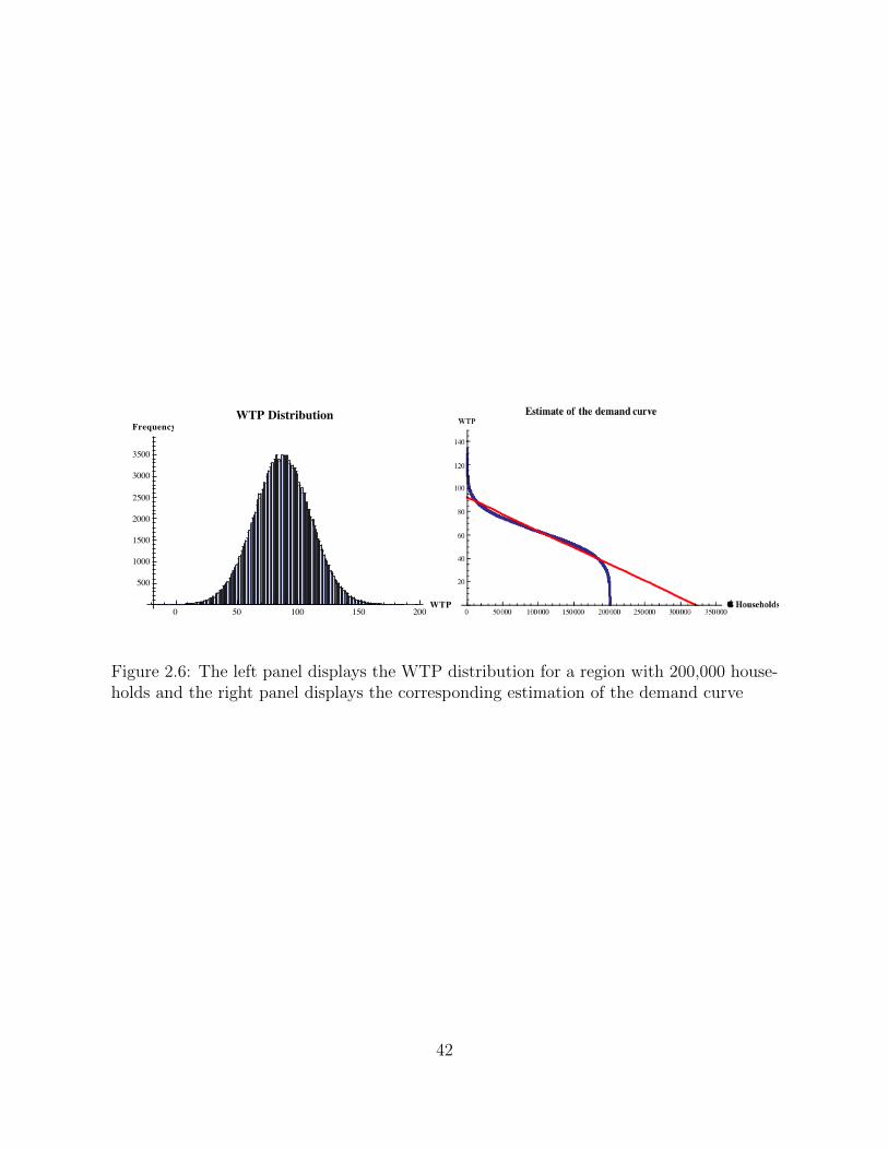
0 50 100 150 200WTP

500

1000

1500

2000

2500

3000

3500

FrequencyWTP Distribution

Figure 2.6: The left panel displays the WTP distribution for a region with 200,000 house-holds and the right panel displays the corresponding estimation of the demand curve

42

Chapter 3

Peer Influence in Product Diffusion

over Very Large Social Networks

Abstract:This paper studies the effect of peer influence in the diffusion of the iPhone

3G across a number of communities sampled from a large dataset from a major European

Mobile carrier in one country. We use instrumental variables to control for potential

correlation between unobserved subscriber heterogeneity and peer influence. We provide

evidence that the propensity of a subscriber to adopt increases with the percentage of friends

who had already adopted. While this result is clearly positive and significant its magnitude

is relatively modest. We estimate that 14% of iPhone 3G adoptions in this carrier were due

to peer influence, after controlling for social clustering, gender, previous adoption of mobile

Internet data plans, ownership of technologically advanced handsets and some heterogeneity

in the regions where subscribers move during the day and spend most of their evenings. We

provide results from several policy experiments that show that with this level of effect from

peer influence this carrier would hardly be able to significantly increase sales by selectively

targeting appropriate early adopters to benefit from viral marketing.

43

3.1 Introduction

The pervasiveness of simple, small and light handsets has changed the way people com-

municate. According to the International Telecommunication Union the penetration of

mobile handsets worldwide grew from 12% in 2000 to 87% in 2011. Smartphones account

for a significant part of this growth and their penetration in the third quarter of 2011 was

29% worldwide, 65% in the US and 50% in Europe (Mobile, 2011). The mobile handset

market is expected to reach $340 billion in revenues by 2015. Smart-phones are expected

to account for 75% of these revenues, which represents an increase of 24% per year from

the $85 billion registered in 2010 (marketsandmarkets.com, 2011).

Handsets became like small computers in recent times. Accordingly, their value shifted

towards the software and the data services provided (Economist, 2011). As a consequence,

manufacturers have been increasingly bundling handsets with applications that generate

positive network externalities. Examples of nascent markets for these applications include

Apple’s App Store and the Android Apps. Applications such as FaceTime for the iOs

Apple or Google Talk for the Android allow users to video call over the Internet at no cost,

but they require users to own an Apple device or an handset running the Android OS,

respectively. Therefore, the utility derived from using these applications, and therefore

these handsets, increases with the number of users that do so.

Following the seminal insights provided in (Rohlfs, 1974) and (Katz and Shapiro, 1986)

the role that network externalities play on product demand has been widely developed in

the literature. The standard perspective is that for products that generate positive network

externalities, the overall installed base of users of a certain product increases the expected

44

utility that consumers will derive from a certain purchase decision (Farrell and Saloner,

1985).

For some products, such perspective is realistic. Examples include the case study of

automated teller machines (ATMs) in the United States where network effects are the con-

sequence of accessibility (consumers benefit from their bank having a large ATM network

and the largest the network the higher the consumer’s expected utility) (Saloner and Shep-

ard, 1995), or the case of spreadsheet software where network externalities emerge from

the most used software benefiting from a broader range of training materials, compatible

products as well as increasing likelihood of vendor accessibility (Brynjolfsson and Kemerer,

1996).

However, for mobile communication products, it is likely that peers rather than the

installed base of users will determine the extend of utility changes that each consumer

faces when some other member of the social systems adopts the technology. Take the case

of mobile carrier choice when the price of calls between subscribers of the same carrier is

lower than the price of calls spanning multiple carrier networks. In such contexts users

will have incentives to join the provider that the majority of their regular calling parties

use, but they will be indifferent to the behavior of a random individual whom they never

expect to call (Birke and Swann, 2005, 2007, 2010). A similar situation occurs in the

case of consumer churn in mobile carriers where it has been observed that users tend to

engage in herd behavior mimicking the actions of those with whom they interact frequently

(Dasgupta et al., 2008; Dierkes et al., 2011).

Peer influence has been shown to play a significant role in contexts as varied as student

45

academic performance (Sacerdote, 2001; Carrell et al., 2009; Boucher et al., 2010), smoking

and drinking behavior (Case and Katz, 1991; Mercken et al., 2010), on sexual conduct

(Romer et al., 1994), in the diffusion of trade unions (Hedstrom, 1994), on vaccination

decisions (Rao et al., 2007), the diffusion of new drugs (Coleman et al., 1966; Burt, 1987;

Strang and Tuma, 1993; Valente, 1996a) or physician’s adoption of electronic health records

(Zheng et al., 2010). Yet, the role that social networks and peer influence play in the

diffusion of telecommunication products, and of handsets in particular, is a topic still

largely unexplored. Exceptions include the investigation of peer influence in the diffusion

of video-conference technology (Tucker, 2008), the diffusion of a mobile application that

delivers personalized news (Aral et al., 2009) or the diffusion of call ring back tones (Ma

et al., 2010).

However, the data on data on cell phone activity that mobile companies own, can be

used to trace the diffusion of handsets across social networks. These datasets allow for

understanding which types of handsets benefit more from word of mouth and who are the

users that can exert more influence over their friends to purchase new handsets.

In this paper, we use a large dataset from a major European Mobile Carrier (EURMO)

in one country to determine the role of peer influence in the diffusion of the iPhone 3G.

EURMO is the leader in mobile communications in this country with a market share of

roughly 50%. The iPhone 3G is a conspicuous and expensive handset which are product

characteristics that are likely to make peer influence a relevant player in the diffusion

process(Childers and Rao, 1992).

Such information is valuable for firms because knowing whether the sales of a particular

46

handset can benefit from strong peer influence may be used to design better marketing

strategies. While it is clear that reaching a critical mass of early adopters is fundamental

to compete with products that exhibit network externalities, when peer influence plays a

significant role in the diffusion of such products, companies do not want to target just any

early adopters. They want to focus primarily on the early adopters that are more likely to

be able to influence their friends to also purchase the product. If, however, peer influence

has only a small effect on sales, then companies might be better off with mass marketing

campaigns instead of targeted advertising.

To answer such questions we look, ex-post, at the percentage of iPhone 3G sales by

EURMO that can be attributed to peer influence and we discuss what the company could

have done to further increase sales had it known the impact of peer influence on sales

beforehand.

A major difficulty in our study is that individual unobserved heterogeneity can be

correlated with the adoption decision of the iPhone 3G. If that is the case, homophily -

the tendency that individuals have to be connected to those who are similar to themselves

(McPherson et al., 2001) - may trigger correlations between the variables that capture the

amount of exposure to the iPhone 3g that each individual obtains from its peers and the

unobservables.

To control for correlated effects we use instrumental variables (IV) which we construct

using the complete structure of our large communication graph.

Still, because latent homophily may be simultaneously correlated with the behavior of

interest and also determine the tie formation/dissolution among the members of the social

47

system, we follow a suggestion by (Shalizi and Thomas, 2011) and identify communities of

users within the large communication graph. We then use the information of community

membership to explicitly control the latent unobservables that are likely to be shared

among the members of the same user group as well as to capture unobserved group effects

in the spirit of (Manski, 1993) that can lead to the adoption of this particular handset.

Another advantage of extracting community membership information is that it allows us to

to adjust the standard errors of the inference procedures for within community correlations

rather than falsely assuming independence across the observations in our sample.

We also use Stochastic Actor-Based Models for the Co-evolution of Network Dynam-

ics and Behavior (SAMCNDB) (Snijders et al., 2010) that allow for modeling network

formation and behavior as they jointly co-evolve over time to test the robustness of our

instrumentation approach. We achieve this by independently fitting SAMCNDB models to

each of the communities identified in our sample and computing a summary effect through

meta-analysis (Hedges and Olkin, 1985) which we then compare to the results we obtain

using IV.

Our contributions are of value for the industry and academia.

In one-hand we develop empirical knowledge on the particular case of handset diffusion

over social networks. We show that the propensity of iPhone 3G adoption increases with

the number friends that purchase this same handset. Such result is positive and statisti-

cally significant, but its economic impact was modest. We estimate that 14% of iPhone

3G adoptions in EURMO were due to peer influence, after controlling for social clustering,

gender, previous adoption of mobile internet data plans, ownership of technologically ad-

48

vanced handsets and some heterogeneity in the regions where subscribers move during the

day and spend most of their evenings.

Furthermore, we show that considering the impact of the peer influence effect on the

diffusion process, the effectiveness of a potential viral marketing intervention would be

small. We provide results from several policy experiments and sensitivity analysis that

show that traditional degree and betweenness based targeting strategies of viral marketing

would hardly be economically viable for EURMO to put in practice.

Finally we also provide an empirical framework for the identification of peer influence

in observational studies that can be readily extended and applied to other situations in-

volving large social networks. In particular, to the best of our knowledge, we are the first

authors to use community identification algorithms (widely developed in the literature of

social networks) to control for latent homophily and correlation among the observations in

the sample and we also provide a methodology for applying SAMCNDB models to large

networks using tools from the social networks and the clinical trials literature.

This paper has nine sections. Section 3.2 provides a review of relevant literature and

positions our paper and contributions in the field. Section 3.3 discusses the introduction

and the diffusion of the iPhone 3G in the country studied and describes our dataset. Section

3.5 presents our empirical strategy and section 3.6 provides our results for the impact of

peer influence in the diffusion of the iPhone 3G in the country under analysis. Section

3.7 provides several robustness checks of the results. Policy simulations are discussed in

section 3.8 and we conclude in section 3.9.

49

3.2 Literature Review

3.2.1 Diffusion and Peer Influence

The term diffusion denotes the dissemination of some trait, product or characteristic within

a social system (Strang and Soule, 1998). It is generally characterized by four elements

which are the social system comprised of the individuals, the groups and the institu-

tions that are potential adopters, the channels of communication that are the means

through which the members of the social system obtain information and discuss the ele-

ment being diffused - which we will refer to loosely as the innovation - and time that

relates to the rate at which adoption takes place (Mahajan, 1985, page 7).

Diffusion can be caused by external influence processes, by mechanisms internal to

the social system or by a conjugation of both. When diffusion is caused by external

sources it is usually because forces such as the mass media broadcast information about

the innovation of interest and such information compels the members of the social system

to adopt (Valente, 1996a, page 81). Other external mechanisms of diffusion exist and they

include policy impositions, or other societal level events that could compel or force the

adoption behavior (Mahajan, 1985, page 15)(Valente, 1996a, page 95).

Alternatively, diffusion may be the result of mechanisms internal to the social system

that will cause individual adoption behavior to be dependent on the adoption behavior of

other members of the same system (Strang, 1991). These are the mechanisms that we are

concerned with in this paper.

Peer influence, social influence, influence or contagion, are terms used in this paper

50

interchangeably to denote the dyadic process that takes place when an individuals shapes

his own behavior, beliefs or attitudes according to what other actors in the same social

system think, express or how they behave (Leenders, 2002).

In the context of diffusion, peer influence is the micro-level manifestation of a broad

range of mechanisms internal to the social system which include, but are not limited to

product network externalities in the sense provided in the previous section that have been

a core concern in the telecommunications’ related research thus far.

(Strang and Soule, 1998; Van den Bulte and Lilien, 2001; Leenders, 2002) list the main

sociological mechanisms that can drive peer influence.

Such mechanisms include Information transfer when members of the social system get

to know about the innovation by direct or indirect communication with previous adopters

(Katz and Lazarsfeld, 1955), competition which occurs when individuals look at their rivals

as frames of reference. Rivals are typically defined as those connected to similar others

than the ego (structural equivalent actors) (Burt, 1987). Conformity that depends on

group values and norms and it assumes that individuals comply to the behaviors and atti-

tudes of the groups to which they belong (Menzel, 1960). Network externalities when the

utility of adopting a particular innovation increases with the installed-based of adopters,

the members of the social system who decide to adopt will also benefit from further adop-

tions (Katz and Shapiro, 1994) and Spatial Proximity since geographically proximal actors

tend to influence each other even if there is no particular explanation for why that is so

except that spatial proximity facilitates all types of interactions (Strang and Soule, 1998).

Empirically such differentiation is usually impossible (Van den Bulte and Lilien, 2001),

51

therefore, in this paper, we are concerned with a broad concept of influence in which all

the mechanisms laid out above can play a part which we do not attempt separating. Our

concern in this research is to quantify the weight of peer influence in the adoption decision

of product in a social network inferred from communication links, but we will make no

claim as to what mechanism is really driving such influence process.

3.2.2 Related Studies

Our paper is part of a vast literature of observational studies that characterize the dif-

fusion of innovations. Early work in this field puts forward that people contemplate the

experience of others before deciding whether to adopt a novel product. The idea is that

interactions between adopters and non-adopters mitigate the risk and uncertainty associ-

ated with novelty (Rogers, 1995). A common theme is the characterization of the diffusion

process using a Bass Model (Bass, 1969) or any of its variants surveyed in (Mahajan, 1985;

Mahajan et al., 1990) that assume that every individual in the population can influence

any other member of the same social system.

In our paper, we look at individual level connections as the source of social influence

rather than the installed based of adopters. Like (Granovetter, 1978; Granovetter and

Soong, 1983, 1986, 1988) our hypothesis is that the likelihood of adoption is linked to

the level of exposure to the innovation, with exposure defined as the proportion of people

in one’s social circle that have already adopted (Valente, 1996a). However, unlike those

authors who are concerned with establishing individual level thresholds of exposure above

which individuals decide to adopt, our research is concerned with characterizing the average

52

marginal impact that additional adopters of the iPhone handset in the ego network of each

subscriber have in the individual probability of adoption.

How innovations diffuse depends on the actual characteristics of the product of interest

(Rogers, 1995), therefore, studies of how social influence affect the diffusion process are

situation and context specific. To the best of our knowledge, we are one of few authors

characterizing the impact of peer influence in telecom products and we are the first to do

so for the case of handsets. A few previous studies have focused on the diffusion of mobile

phones, but for the purpose of explaining the penetration of wireless communications and

not to characterize how particular handsets spread. Examples of such studies include

(Gruber, 2001) for the diffusion of mobile communications in Eastern European, (Botelho

and Pinto, 2004; Carvalho, 2006) for the Portuguese case,(Doganoglu and Grzybowski,

2007) for Germany (Singh, 2008) in India, (Chu et al., 2009) for Taiwan and (Park and

Ueda, 2011) in Korea and Japan.

Our study is also related with the methodological literature on the identification of peer

effects in social networks that was developed following the seminal work of (Manski, 1993).

Manski’s research highlighted the difficulties of identifying the effect of group behavior

on individual choices when (1) it is impossible to identify the reference groups for each

individual in the social system; (2) there are unobservables that can cause correlated

outcomes as well as influence the formation of links between members of the social system;

and (3) there exists simultaneity in the behavior from ego and alters.

The identification of reference groups became possible through data collection strategies

that capture the structure of the relations among the members of the social system (the

53

social network). Such data allows determining who influences whom (Wasserman and

Faust, 1994; Bramoulle and Fortin, 2009). In several domains, collecting this type of

information is costly or even impossible and so far, only a handful of studies have used

large real world networks to analyze how peers affect each other in societal level networks

(Aral et al., 2009).

In this paper we use a large network from a market leader in mobile telecommunications

services in one country whose clients make up for approximately half of the population of

that country. In itself, the analysis of large network data is a relevant contribution for the

diffusion of innovations literature. This is so because small network data contains only

a small sample of the population and most often a non-random sample since due to ho-

mophily, social networks tend to clustered in homogeneous groups of individuals (McPher-

son et al., 2001). Additionally, individuals in small networks are also likely to be part of

larger networks and in studies of small networks, such a fact, and its strong implications,

are never discussed. (Anagnostopoulos et al., 2008) and (Aral et al., 2009) have analyzed

the problem of innovation diffusion in large social networks, but their research focused on

the spread of free of charge products in a context completely distinct from ours.

Correlated effects and simultaneity have been tackled in several distinct ways.

The preferred course of action is the use of randomized control trials. (Aral and Walker,

2011) and (Bapna and Umyarov, 2012) are notable examples of studies that do so in large

scale networks.

The former uses a Facebook.com application that allows its users to share comments

related to the film industry. The application has the ability to send messages to each Face-

54

book.com friend of the adopter individual. The results of the study show that the ability

of viral messaging within the application created contagious adoption among the millions

of Facebook.com friends of a set of 9,687 individuals that were recruited to participate in

the experiment.

The latter uses Last.fm, website for music sharing. The authors test the hypothesis

that users connected to others who pay for premium services provided by Last.fm will be

influenced to adopt these paid services themselves. By awarding free subscriptions to a

randomized set of users, (Bapna and Umyarov, 2012) are able to show that the odds of

subscribing the premium service increase by up to 50% due to the influence generated by

a friend who adopted the service.

The two above mentioned studies are at the frontier of IS research, however, in markets

of physicals goods that are expensive, it is unlikely that similar opportunities for experi-

mentation in large scale networks will emerge frequently. There is the obstacle of deriving

the social network of interest of the parties involved and the actual cost that such efforts

would entail. While the marginal cost of a Last.Fm subscription is likely to be negligible

for the provider, in the case of the iPhone 3g, for example, it would cost hundreds of thou-

sands of dollars to distribute a few thousands of phones in the population. Providers will

not engage in such initiatives unless they expect to profit in return.

So far, the knowledge on social influence does not yet permit predicting and controlling

the flows of social influence in real world networks (Aral, 2012) and many more experi-

mental and observational investigations will be needed until we reach that far, thus the

identification of ways to deal with the problems of simultaneity and correlated effects in

55

social networks are still very much needed.

In observational studies, simultaneity can be solved using instrumental variables in

peer effect models (Lee, 2007; Bramoulle et al., 2009; Oestreicher-Singer and Sundararajan,

2010; Lee et al., 2010) or through instrumental variables derived from natural experiments

(Sacerdote, 2001; Tucker, 2008). Correlated effects due to unobservables that determine

behavior can be controlled using fixed effects methods (Lin, 2010). Alternatively, matching

in high resolution panel data settings, can also be used (Rubin, 1973; Hill et al., 2006; Aral

et al., 2009) to deal with these problems.

Natural experiments are rare and peer effect models and matching can break in the pres-

ence of unobservables that simultaneously determine tie formation and behavior (Shalizi

and Thomas, 2011). Instruments derived in peer effect models rely on the structure of the

social network so they require that network ties are exogenous to the behavior of interest.

Matching estimators assume that treatment assignment is strictly ignorable conditional on

a set of observed explanatory variables and they also assume that individuals belong to

the treated or the control group with positive probability (A. Smith and E. Todd, 2005).

In this paper we differentiate from the previous approaches by using instrumental vari-

ables, but at the same time controlling for community membership of the individuals of

our population of interest.

The community membership controls emerge as an attempt to capture part of the

unobserved traits that simultaneously determine the adoption behavior and the actual

links that that tie individuals together.

Homophily suggests that social networks will tend to be formed of homogeneous clusters

56

of individuals sharing similar values of the unobserved traits (Aral et al., 2009). Therefore,

as suggested in (Shalizi and Thomas, 2011) controlling for community structure may help.

The assumption is that the communication graph used to infer the social network structure

of the subscriber set provides sufficient information to uncover the group membership of

each subscriber conditionally independent on the observed adoption behavior. In other

words, the community membership captures the part of the unobservables that determine

the network structure, leaving out only those latent characteristics that influence behavior,

but that do not determine the formation of ties among individuals.

Communities, as defined in (Newman, 2004), are clusters of individuals who speak more

time amongst each other than to the rest of the network as a whole. They can be identified

with community detection algorithms that have been widely developed in the literature

and surveyed in great detail by (Fortunato, 2010). We test several community detection

algorithms in this paper and report our conclusions regarding to which methods are most

promising to the task at hand.

Additionally, because we identify communities in the social network we are also able

to go a step further and test the robustness of our results using Actor Based Models of

network dynamic co-evolution and behavior.

Such methods use agent-based simulation models to describe the dynamics of link

formation across members of a social network and the relationships between the emerging

social network structure and behavior (Snijders et al., 2010). This class of models separate

the contributions of homophily and influence for the diffusion of a certain practice through

the social network by estimating network structure and behavior jointly (Steglich et al.,

57

2010). Because of computational complexity, and the assumption that each member of the

social system is a suitable candidate to befriend any other member, this approach does

not scale well to large networks (Aral, 2010). Furthermore, providing interpretation with

economic meaning to the estimate of the parameters of interest is far from straightforward

(Ripley and Snijders, 2010). However, due to our community identification strategy we

are able to fit these models to small networks within the large communication graph that

respect both the theoretical assumptions as well as computational requirements of the

algorithm.

Finally our work is also related to the literature on viral that is emerging as a response

to consumers’ overwhelm with information about new products and services (Hinz et al.,

2011) and avoidance of the traditional marketing instruments (Hann et al., 2008). Viral

marketing campaigns assume that information about products is generated and spread by

consumers among themselves starting from a small set of initial adopters called the seed

(Leskovec et al., 2007; Bampo et al., 2008).

Leveraging on the estimates for average partial effect of the peer influence on the

individual probability of adoption of the iPhone 3g, we test how different seeding strategies

that are frequently considered in the viral marketing literature could have been used by

the operator to increase sales. In particular we test whether targeting well connected

individuals (Goldenberg et al., 2009), bridges (Granovetter, 1973; Watts, 2004) or well

connected individuals that are far apart from each other in the social network (Watts

et al., 2007) could have benefited the spread of the iPhone 3g in the population.

Our results show that targeting hubs and bridges in the social network performs better

58

than randomly seeding, however, they also highlight that the marginal benefit of such

strategies will be low unless the virulence of the product itself is high. We show that when

the cost of seeding is non-trivial, companies may have little incentive to engage in viral

marketing unless the content of the product itself favors its own diffusion through the social

network.

3.3 The iPhone 3G and the EURMO dataset

3.3.1 iPhone 3G Release

The iPhone 3G was released in 2008 as the first Apple smartphone commercialized in the

country under analysis 1. People in that country spent on average 20 Euros per month in

mobile communications during 2008. The median was 15 Euros per month. NOKIA was

the preferred mobile phone brand in that country with a market share above 40%, followed

closely by Samsung. LG and SONY had market shares below 10%. Overall, smartphone

sales were still incipient in that country accounting for a mere 11% of the yearly handset

sales. Figure 3.1 shows that ease of use, price, size and weight were among the most

important factors that consumers considered when buying a handset2.

1The country analyzed is not disclosed for protection reasons. All numbers in this section were providedby a major consulting company operating in this country that regularly runs market surveys

2The price of the iPhone 3G at launch in this country was 500 (600) Euros for the 8Gb (16Gb) versionwithout a contract with a provider. Alternatively, the iPhone 3G could have been purchased at a reducedprice with a contract with one service provider. Prices varied between 130 Euros and 400 Euros dependingon the type of contract selected. Contracts lasted at least 24 months and significant penalties appliedto terminate a contract before expiry. Both with and without contract, the iPhone 3G was sold with asoftware lock to the service provider selling the device. The lock could be released at no charge after 24months. Consumers willing to release the lock before 24 months would need to pay a 200 Euro charge.Communication contracts associated with the iPhone 3G varied slightly across service provider. Theyranged between 30 Euros and 65 Euros per month

59

The iPhone 3G was a conspicuous luxury product. It was expensive, innovative and

users could only benefit from its full potential if they subscribed to a data plan. There

was a clear mismatch between what the average user expected from a handset and the full

set of features offered by the iPhone. All such factors were likely to generate uncertainty

and motivate consumers to seek the opinion of others before making a purchase decision

(Childers and Rao, 1992).

Our hypothesis is that peer influence was a positive determinant of iPhone 3g sales and

that the more of one’s friends adopted the handset, the more likely it would be for the ego

to adopt as well.

Figure 3.1: Most important characteristics considered when purchasing a new handset (%of total respondents who named each particular characteristic)

60

3.3.2 Raw Dataset

Our dataset includes communication data between August 2008 and June 2009. The

iPhone 3G was released in July 2008 by EURMO. For every call originated or received

by a EURMO subscriber we have the anonimized phone numbers of the caller and the

callee, the cell towers they used to call each other, a timestamp for when the call took

place and the duration of the call. We also have the GPS coordinates for all cell towers in

EURMO. For every sms sent or received by a EURMO subscriber we have the anonimized

phone numbers of the caller and the callee. We also have a set of subscriber characteristics

including date of birth, gender, zip code for the account owner, type of contract, tariff plan,

add-on services such as ring tones, free weekends, packs of sms, handset and changes over

time for all these characteristics. We have 16.5 million phone numbers in our database, 3.7

billion calls and 13 billion of sms.

3.3.3 Social Network

We use the dataset described above to define an undirected graph of communications across

EURMO subscribers over the entire period of analysis. We trim subscribers from other

mobile operators because we do not have their account information and therefore we cannot

know, for example, whether they adopted the iPhone 3G.

An edge between two users is added to our graph if one of them called or sent an

sms to the other and the latter answered back with a call or an sms within the same

calendar month. This procedure disregards communications that are unlikely to proxy

social proximity such as those involving message bots, short numbers and call centers as

61

well as non reciprocal communication across regular subscribers.

We also remove from our dataset numbers that at some point in time were owned by

multiple subscriber accounts (called recycled phone numbers), as well as numbers whose

subscribers switched between pre-paid and post-paid because in both these cases we cannot

accurately track their history. These two cases eliminate less than 5% of the EURMO active

subscriber base.

Finally, we trimmed from the dataset subscribers whose out-degree was more than 3

standard deviations above the mean. This removes PBX machines and ensures that the

size of our graph is computationally manageable. This eliminates less than 1.6% of the

subscribers in our graph.

In the subsequent analysis we use the term friends to identify people who contact

each other and are thus connected with an edge in our communication graph. Our final

communications graph includes 4, 986, 131 subscribers and 57, 069, 798 undirected edges.

The undirected graph density is 4.59 ∗ 106 and the mean number of friends (degree) is 22.9

with a standard deviation of 25.5. The median number of friends is 13. Figure 3.2 plots

the distribution of the number of friends.

3.4 Community Based Sample

Communities are defined as groups of individuals whose members have dense connections

within the group and only sparse links to individuals outside the group (Newman, 2004).

Peer influence is a local phenomena. It occurs when alters play a part in the ego’s

decision process (Leenders, 2002). As mentioned above, the social network that we use

62

Figure 3.2: Empirical degree distribution of our communications graph. Grey dots repre-sent subscribers whose out-degree is three standard deviations below the mean

in this analysis includes 4.9 million subscribers that are sparsely connected. As such, it

is likely that influence flows will occur within local clusters of this large network and not

span across the entire population of subscribers.

Homophily suggests that social networks will tend to be formed of homogeneous clusters

of individuals sharing similar values of unobserved traits and this is a central concern

of most studies of contagion (Aral et al., 2009). To minimize the bias introduced by

63

the confounding effects of latent unobservables we uncover such clusters of users through

community identification algorithms as was first suggested in (Shalizi and Thomas, 2011).

The underlying assumption is that community membership will tend to capture part of the

unobservables that determine the network structure and that could simultaneously derive

behavior.

A further advantage of community identification is that it allows to separate user com-

munities with no adoption events, from those where at least one member adopted the

iPhone 3g. To understand why such possibility is important consider an example from

epidemiology.

Suppose that there is a disease called pox and that there are two separate populations of

users of he same size. Population p1 is completely immune to the disease while population

p2 is vulnerable. If one tried to estimate the virulence of pox within population p1 by

introducing sick individuals into p1, the conclusion would be that pox is not contagious.

However, if the same experiment was repeated in p2 the analysis would allow determining

the rate at which the disease spreads. If p1 and p2 were analyzed as a single population

the virulence of pox would be underestimated.

In the market place, companies segment clients into different categories and they try

to sell different product versions or even distinct products to different consumer segments.

Segmentation reflects the adjustment of products and marketing effort to consumer or user

requirements(Smith, 1956). Therefore, knowing the size of the influence effect in the pop-

ulation of susceptible is more valuable to the firm, than when the effect is averaged over

the immune.

64

Communities in which at least one adoption occurred are more likely to represent

clusters of susceptible individuals than communities with no adopters.

Finally, community identification also allows working with a smaller part of the social

network by permitting us to use a sample of cohesive groups of users that are independent

from each other. If such clusters are identifiable, then they can also be used to correct the

standard errors of regression procedures which will also be biased when dealing with social

network data. Such fact is usually ignored in most empirical work, which tends to assume

independence across sample units which in social networks is impossible by definition.

3.4.1 Community Identification Algorithms

The physics and social network literature are rich in community identification algorithms

for which excellent and in-depth surveys are provided in (Lancichinetti and Fortunato,

2009; Fortunato, 2010). Table 3.1, which we adapted from (Fortunato, 2010), lists a wide

range of algorithms of this kind.

A majority of the community identification algorithms listed in the table have compu-

tational complexities that make them impossible to use in networks as large as the one that

we use in this investigation. The computational complexity provided in the last column of

the table is for the worst case scenario, but (Pons and Latapy, 2006; Lancichinetti et al.,

2008; Lancichinetti and Fortunato, 2009) show that the first ten alternatives listed in table

3.1 are not capable of processing a social network with 4.9 million nodes and 57 million

edges.

65

Taking this into consideration we focus on algorithms 11 through 173. We summarize

the mechanics of each algorithm in appendix 3.C.

Table 3.1: Community Detection Algorithms and Their Computational Complexities# Authors Reference Computational

Complexity1 Palla et. al. (Palla et al., 2005) O(exp(n))2 Newman & Girvan (Newman and Girvan, 2004) O(m2n)3 Girvan & Newman (Girvan and Newman, 2002) O(mn2)4 Furtunato et al. (Fortunato et al., 2004) O(n4)5 Bragow & Bollt (Bagrow and Bollt, 2004) O(n3)6 Donetti & Munoz (Donetti and Munoz, 2005) O(n3)7 Zhou & Lipowsky (Zhou and Lipowsky, 2004) O(n3)8 Duch & Arenas (Duch and Arenas, 2005) O(n2log(n))9 Radicchi et. al. (Radicchi et al., 2004) O(n2)

10 Newman (Newman, 2003) O(n2)11 Zhang et.al. (Zhang and Krackhardt, 2011) O(n2c(nc + nb))12 Latapy & Pons (Pons and Latapy, 2006) O(n2log(n))13 Clauset et.al. (Clauset et al., 2004) O(nlog2(n))14 Wu & Huberman (Wu and Huberman, 2004) O(m+ n)15 Raghavan et.al. (Raghavan et al., 2007) O(m+ n)16 Blondel et.al. (Blondel et al., 2008) O(m)17 Rosvall & Bergstrom (Rosvall and Bergstrom, 2008) O(m)Note 1: Adapted from (Fortunato, 2010) Note 2: n denotes the number of nodesin the social network, m denotes the number of edges in the social network, ncdenotes the target number of nodes in the sub-population of interest nb denotes thenumber of nodes in the boundary of the sub-population of interest.

The overall adoption rate of the iPhone 3g was less than 1% therefore, if we sample

very small communities of users, it is unlikely that we will be able to find clusters within

which at least some individuals purchased the phone. Because of this, we aim at identifying

groups of individuals with about 100 members, which according to Leskovec et al. (2009)

is the size about which clusters tend to start blending into the very large graph from where

they are sampled and are unlikely to represent real social clustering.

3We ignore algorithms 14 and 15 described in (Wu and Huberman, 2004; Raghavan et al., 2007) becausewe could not find publicly available software implementations. The authors of (Raghavan et al., 2007)kindly provided us with their implementation in JAVA, but the software would not directly run in ourdata. For this algorithm, the igraph0 package (Csardi and Nepusz, 2005) also contains an availableimplementation. However, the library code has a data structure problem and it takes O(n2) rather thanO(n + m) to run. We actually attempted to use the iGraph0 version of the software, but after 4 monthsof runtime we stopped the algorithm with no output at all

66

3.4.2 Community Identification

Table 3.2 contains the output of the different algorithms used.

More than 50% of the groups identified by the different algorithms have at most two

subscriber members and no adopter individuals. Such communities are irrelevant for our

analysis which goal is to find cohesive clusters of individuals that are likely to share the

same value of unobservables. Additionally, the proportion of total subscribers assigned to

communities with sizes larger than 100 individuals is 63.2% for the Walktrap (Pons and

Latapy, 2006), 99.5% for the Louvain’s method (Blondel et al., 2008), 99.6% for Infomap

(Rosvall and Bergstrom, 2008) and 98.2% for Clauset (Clauset et al., 2004; Clauset, 2005).

Therefore, an overwhelming majority of subscribers was placed in communities that due

to their large sizes are unlikely to entail social meaning (Leskovec et al., 2009).

Besides TCLAP, (Pons and Latapy, 2006) produces better results than the remaining

algorithms, however, as table 3.3 highlights, the number of communities identified by this

algorithm that have adopter individuals is quite limited.

With these results for the different community algorithms we choose T-CLAP to pro-

ceed our analysis to which we devote further attention in the next section.

Table 3.2: Summary of the community identification algorithms outputAlgorithm Edge Execution Number of Community Size

Weights Time Communities Min Median Max MeanLatapy & Pons Yes 1 week 977,999 1 1 488,471 5.0Blondel et.al. No 3 hours 8,417 2 2 886,764 592.4Rosvall & Bergstrom No 4 hours 8,113 2 2 1,564,858 614.6Rosvall & Bergstrom Yes 4 hours 8,081 2 2 2,490,201 617.6Clauset et.al. Yes 1 month 25,373 2 2 317,426 179.3Zhang et.al. Yes 3 weeks 2,134 2 103 115 96.7Note 1: Unlike the other algorithms used T-CLAP does not process the entire social graph. Itlooks for local community focusing on small parts of the social network at a time.

67

Table 3.3: Communities identified with 25 ≤ communitysize ≤ 200Algorithm Number of Communities with Total Number of Adopters per Community

Communities Adopters of Adopters Mean Min Median MaxLatapy & Pons 2,996 313 447 0.149 0 0 8Blondel et.al. 47 3 8 0.179 0 0 6Rosvall & Bergstrom 24 2 2 0.018 0 0 1Rosvall & Bergstrom 14 0 10 0.000 0 0 0Clauset et.al. 232 27 37 0.159 0 0 3Zhang et.al. 2134 1936 72,995 36.51 0 16 115Note 1: Number of T-CLAP communities before discarding overlaps

3.4.3 T-CLAP community sample

T-CLAP extracts random communities in three steps: (1) it selects one node at random

and collects a sample of nodes and edges through breath first search; (2) applies a clus-

tering procedure to the collected nodes to identify dense regions within the sample; (3)

sequentially discards nodes that have more links to outside the community than inside,

as measured by the individual Internal External Ratio (IER) until a certain community

size is obtained. The IER is an adaption from the E-I index proposed in (Krackhardt and

Stern, 1988) and is detailed in equation 3.1:

IER =I − EI + E

(3.1)

In this case, I denotes the number of calls and sms exchanged across community mem-

bers and E denotes the number of calls and sms exchanged between community members

and individuals outside the community. IER varies in [−1; 1]. The lower bound is attained

when the community members communicate only with members outside the community.

The upper bound is attained when community members do not communicate with mem-

bers outside the community. A community with a higher IER is more isolated from the

68

rest of the network graph. The higher the IER the more isolate the community. Commu-

nities with negative IER imply that its members as a whole interact more often with other

individuals outside the community and is an indication of poor grouping.

Because iPhone adoption was a rare event, the chances of any random community of

size smaller to 100 identifying adopter members is low. Unlike the other algorithms that

we tested, T-CLAP looks for local communities in subgraphs of the complete network,

it does not process the entire social graph. This exacerbates the problem of identifying

communities with iPhone adopters, since a global partition of the graph is not provided

by this algorithm.

To accommodate and overcome this problem, the version of T-CLAP used in this paper

was modified from the original algorithm to focus on communities where adoption events

occurred. To increase the performance of the algorithm with respect the identification of

communities with iPhone 3g adopters, we changed T-CLAP in the following three ways:

i) in step (1) we start the snow-ball sample from nodes that adopted the iPhone 3G (we

sample 4 waves out); ii) we skip step (2) altogether; iii) in step (3) we prune iPhone 3G

adopters with lower probability. If two subscribers have the same IER, but one of them

adopted the iPhone, we prune the non adopter first.

Our version of TCLAP takes longer to run than the original code because it skips the

clustering phase, but it increases the probability of identifying communities with adopters.

We then use the IER index to evaluate the communities obtained by the modified TCLAP

algorithm.

Other metrics for community evaluation exist, the most commonly used being mod-

69

ularity (Newman and Girvan, 2004). Modularity is an index of the quality of a graph

partition that compares the number of edges within a given group of nodes and the ex-

pected number of edges that such group would have if the network ties were randomly

determined (Newman and Girvan, 2004). Modularity evaluates a partition of the entire

graph into communities. We do not use it in this case because modularity suffers from

a resolution limit (Fortunato and Barthelemy, 2007). (Fortunato and Barthelemy, 2007)

show that when the size of the social network increases, the expected number of edges be-

tween two groups decreases possibly becoming smaller than the unit and the consequence

is that for large graphs, the modularity index will tend to overlook the existence of small,

but non-trivial communities. This is problematic for large networks as our own.

Unlike modularity,IER is agnostic to network size. Additionally, several other theoret-

ical notions are embedded in the IER which are of interest to the identification of cohesive

and homogeneous groups.

IER is a measure of dominance of internal over external connections, it reduces with

the decrease of internal communication, but also with the increase of external communi-

cation (Zhang and Krackhardt, 2011). The time that individuals can devote to maintain

friendship and intimacy through to social interaction is limited and the IER captures the

trade-off between the attachment to the group and the relationships that one is able to

maintain outside (Krackhardt and Stern, 1988). By comparing internal against external

links, the IER also controls for heterogeneity in the amount of time that individuals devote

to communication and to the number of connections that they maintain. People who inter-

act with more people and more frequently are likely to do so internally and externally and

70

the reverse is also true for individuals who engage in fewer communication interactions.

Because the IER is reported as a ratio, it is not the absolute number of interactions, but

rather the balance between internal and external communications that is factored when

analyzing the attachment of any individual to a group.

To select our community sample we require that communities have a positive IER index

and we exclude from the sample groups of individuals that overlap. From the 2,134 com-

munities that we obtained with the TCLAP algorithm only 263 match these two criteria.

These communities have 24,131 subscribers of which 1,758 adopted the iPhone 3G 4.

Table 3.4 extends the calculation of the IER index to the communities generated by the

remaining algorithms. It again reinforces the idea that TCLAP is the most appropriate

algorithm for the task at hand.

Table 3.4: Non overlapping communities with 25 ≤ communitysize ≤ 200 and positiveIERs

Algorithm Communities Total Adopterswith IER > 0

Latapy & Pons 70 15Blondel et.al. 46 8Rosvall & Bergstrom 20 2Rosvall & Bergstrom 10 0Clauset et.al. 21 0Zhang et.al. 263 1,758

Besides having positive IERs and being non-overlapping, the 263 communities that we

obtained are also very much disconnected from each other in the actual social network. To

determine the extent of community separation we perform two distinct tests.

The first separation measure consists in calculating geodesic distances between users

who belong to different communities. We select two communities randomly and we se-

4We chose the communities in random order and when two communities have overlapping individualsand positive IER we keep the first community that we sampled and discard the latter.

71

lect one user randomly within each community chosen. Finally we compute the shortest

path between the users within the entire communication graph. We repeat this procedure

500, 000 times. We find that the mean distance across random pairs of users in distinct

communities is 4.76 edges with a standard deviation of 0.66 and figure 3.3 depicts the em-

pirical distribution of the length of the geodesics between random pairs of users in distinct

communities.

Figure 3.3: Path between subscribers in distinct communities

Additionally we look at the extreme cases. We look for subscribers at the edge of each

community that may be linked directly to members of other communities in the sample.

To do so, for each community extracted using T-CLAP, we perform a breadth first search

of depth one in all members of that community. Such operation allows identifying the

friends of the community members that are external to the community itself. Using this

information we create an undirected network of the 263 communities with each community

72

representing a node in this network. The community network has a density of 0.07 which

means that out of the 34,453 theoretically possible inter-community ties there are only

2,425 connections between communities. 1,827 of these links are of weight one which

means that the connected communities share a single tie between them. This shows that

communities are not completely isolated from one another, but that they are at most very

sparsely connected.

Finally, Figure 3.4 displays the distribution of the adoptions in the community sample

over the 12 months that we analyze. Figure 3.5 depicts the relationship between the IER

and both community density and community size for the 263 communities analyzed high-

lighting that there appears to be no particular correlation between any of such measures.

73

Figure 3.4: Number of adoptions each month for the subscribers in the sample. The 0in the x-axis indicates the month of July which coincides with the release period of theiPhone 3G handset

Figure 3.5: Communities extracted with the modified T-CLAP algorithm

74

3.5 Consumer Utility Model

At any point in time users choose to adopt or not the iPhone 3G. Let Uit represent the

difference in utility for user i from adopting and not adopting the iPhone 3G at time t. Uit

is defined by the following reduced form equation:

Uit = α +Xiβ + Zitγ + ρWiYt−1 + εit (3.2)

Xi is a set of time invariant covariates, which in our case include gender, subscription of

mobile data plans and the technological sophistication of the handset owned just prior to

the release of the iPhone 3G. Such controls are included because several studies adoption of

technology show that past experience with technologies similar to the innovation of interest

contribute positively to the perceived usefulness of the innovation (Karahanna et al., 2006)

which in turn is known to contribute to adoption (Venkatesh et al., 2003). Gender has

also been reported to play an important role in how individuals perceive that a certain

technology will perform (Gefen and Straub, 1997; Venkatesh and Morris, 2000; Venkatesh

et al., 2003). This set of covariates is summarized in Table 3.5.

Zit is a set of time varying covariates, possibly time lagged. In our case it includes

tenure with EURMO, which may relate to the experience and trust that a subscriber has

with this carrier and therefore can contribute to the probability of adoption of the new

handset from EURMO. Tenure with EURMO is summarized in Table 3.6.

W is an adjacency matrix, Wi is the ith row of such matrix and Yt−1 is a column vector

that stacks the adoption decisions of all individuals up to time t − 1. εit ∼ N(0, 1) is the

75

Table 3.5: Descriptive statistics of time invariant covariatesVariable Description Mean Standard Dev.genderM =1 for male 0.209 0.406genderF =1 for female 0.185 0.388genderU =1 for subscribers who did not re-

port a gender0.605 0.489

prepaid =1 if subscriber i had a pre paidtariff on June 30 2008

0.606 0.489

mobileNet =1 if subscriber i had a mobileinternet on June 30 2008

0.023 0.150

phone2.0g =1 for ownership of 2.0g handseton June 30 2008

0.157 0.363

phone2.5g =1 for ownership of 2.5g handseton June 30 2008

0.478 0.499

phone3.0g =1 for ownership of 3.0g handseton June 30 2008

0.331 0.470

phone3.5g =1 for ownership of 3.5g handseton June 30 2008

0.028 0.166

phoneOther =1 for ownership a handset withunknown range on June 30 2008

0.004 0.066

phoneAge Number of years a subscriberhas used the handset it owns on30th of June of 2008 (before theiPhone 3g release)

0.790 0.716

Note 1: Mean and standard deviations over the subscribers in the sample

Table 3.6: Descriptive statistics of time varying covariatesVariable Description Mean Standard Dev.tenure Number of months a subscribers is using the EU-

RMO provider66.393 43.832

Note 1: mean and standard deviation computed over the entire panel

error term. User i will adopt the iPhone 3G at time t if Uit > 0. Therefore, yit = 1{uit > 0}.

In this model, the terms α+Xiβ+Ziγ capture the individual intrinsic utility from acquiring

the iPhone 3G while parameter ρ measures the contribution of peer influence to adoption.

In this model, if peer influence is positive, adoption increases the number of friends that

adopt, as well as the number of friends of friends that adopt recursively, which in turn

increases the propensity to adopt. In this case, and after a while, the model originates

the well known S-Shaped diffusion curve. If peer influence is negative or very low and the

intrinsic utility to adopt is small, fewer people are likely to adopt and the handset will not

76

spread across the population.

Table 3.7 provides descriptive statistics for variables related with adoption.

Table 3.7: Descriptive statistics for the variables related to adoptionVariable Description Mean Standard Dev.adoptedt =1 if the subscriber i adopts the

iPhone 3g ate time t.0.006 0.079

frd adopterst−1 % of a subscriber’s contacts whoadopted the iPhone 3g up to timet− 1

0.013 0.033

N frd adopterst−1 absolute number of contactadopters up to t− 1

0.412 0.889

Note 1: mean and standard deviation computed over the entire panel; Note 2:Adoption means handset usage for a minimum consecutive period of thirty days

As discussed in (Allison, 1982) and in (Tucker, 2008) the model laid out in equation

3.2 can be empirically estimated with a pooled probit as long as the standard errors are

adjusted to account for error correlation (either through sandwich estimator (Wooldridge,

2002, page 486) or block bootstrap (Efron, 1993, page 3188)) if the data is organized into a

panel and observations after the adoption event are removed from the sample.

However, due to unobserved heterogeneity, the error term in equation 3.2 can be cor-

related with ρWiYt−1. We know from the vast literature in social networks that similar

people tend to be connected to each other (McPherson et al., 2001). When this happens

the unobservables in εitthat can influence one’s adoption are also likely to influence the

adoption of one’s friends, Yt−1. In the case of the iPhone 3G two individuals who are

connected to each other may adopt the iPhone sequentially because of some sales call from

a EURMO representative advertising the iPhone (which we are unable to control for). In

the opposite direction and given its high price, it is also possible that budget constraints

could deter more than one person in the same family to own the iPhone 3G.

77

We start by adding a significant number of dummy variables to control for heterogeneity

that might lead to correlated adoption. We control for three types of heterogeneity, namely

across regions, across subscribers and over time.

First, subscribers living in large cities are likely to face lower search costs because the

iPhone 3G was mainly available from EURMO franchises located in major shopping malls.

Subscribers in large cities might also find it more beneficial to use the iPhone because

part of its functionality requires using the Internet and network coverage in cities is likely

to be better than in rural areas. We use regional dummy variables to control for these

effects. We split regional dummies in two sets. The first set describes the location where

individuals live which we infer from the zip code of the account holder. A second set

of regional dummies identifies the regions where subscribers spend most of their daytime

(8am to 8pm), which we obtain by using the GPS coordinates of the cell towers used to

route calls. We then match regions with statistical information on wages using the last

Census.

Second, the baseline propensity to adopt the iPhone 3G might be different across sub-

scribers. Factors that may lead to such differences that we control for include gender,

the type of contract with EURMO, the characteristics of the handset owned prior to the

release of the iPhone 3G and whether the user had already subscribed to data services

from EURMO as we already presented in tables 3.6 and 3.5.

In addition, and in the spirit of the work by (Manski, 1993), unobservable groups effects

can also drive the adoption of the iPhone 3G and confound our estimates of peer influence.

One example is sets of individuals who communicate frequently within the group because

78

they belong to the same company and this company decides to adopt the iPhone 3G (or

another competing handset for that matter) as the primary handset for its employees.

Alternatively, there could be latent variables determining both the adoption of the iPhone

3g and tie formation as detailed in (Shalizi and Thomas, 2011). To control for these effects

we include community dummy variables.

Third, we add time dummies to control for the fact that the net benefit from adopting

the iPhone 3G changes over time with seasonal promotions, changes in price and similar

policies enacted by EURMO. Table 3.8 summarizes the above mentioned dummy variables.

Table 3.8: Descriptive statistics for the adoption related variablesVariable Description Mean Standard Dev.geoWageV L = 1 if i spends most days in re-

gions 2 standard deviations belowthe average the national average.Regions are studied at municipallevel and daytime is considered toranged from 8:00 to 20:00 for eachday of the 11 month of communi-cations

0.001 0.065

geoWageL = 1 if i spends most days in re-gions were salaries are between 1and 2 standard deviations belowthe national average Regions

0.009 0.095

geoWageA = 1 if subscriber i spends mostdays in regions within 1 standarddeviation of the national average

0.312 0.463

geoWageH = 1 if i spends most days in re-gions were salaries are between 1and 2 standard deviations abovethe national average

0.439 0.496

geoWageV H = 1 if i spends most days in re-gions 2 standard deviations abovethe national average

0.237 0.425

Subscriber/DummyN Dummies Mean Standard Dev.

ZIP Code FE Dummy variables for home zipcode

70 342.3 521.8

Community FE Dummy variables for communitymembership

263 91.7 17.2

Month FE Dummy variables for each month 12 23,064 532.8Note 1: Regions are studied at municipal level and daytime is 8am – 8pm

79

Despite all controls, there might still be unobserved heterogeneity or reverse causality.

To account for such possibility we use instrumental variables.

We start by considering three EURMO users. User j is a friend of user i and user k is

a friend of user j. We want to instrument j’s decision to adopt. One potential instrument

is the adoption decision of user k. The more friends j has that adopted the iPhone 3G the

more likely she is to adopt. The adoption decision of user k, however, might be correlated

with the adoption decision of user i. This might be particularly true if user k and user i

are also friends.

Therefore, we instrument the adoption decisions of the friends of user i with the adop-

tion decision of the friends of friends of user i that are not friends of user i. Call k’ a friend

of user j that is not friend of user i.

Still because of well known sociological processes, such as comparison (Burt, 1980,

1987), one could argue that this instrument might still be endogenous due to indirect

influence from k on i. Therefore, we go a step further to limit that possibility.

We use the GPS coordinates of the cell towers used to route calls to identify the region

where each subscriber spends most of her time. With this information we consider only

users k’ whose primary region is different from the primary region of user i. This ensures

additional separation between user i and the users used to instrument her adoption decision.

Users that spend most of their time in different regions are less likely to influence each

other, particular if there is no additional evidence that such individuals are related in

any way. Note that geographical proximity is known to facilitate interactions (Strang and

Soule, 1998) and that the frequency of face to face and electronic interactions between

80

people tend to decrease as their geographical separation increases (Tillema et al., 2010).

We expect that the instrumental variable just described will perform well to solve the

problem of omitted variable bias and reverse causality because for a subscriber i, the

behavior of the friends of i will likely be correlated with the behavior of the friends of

friends of i due to homophily, which is common in social networks (McPherson et al.,

2001). We note that we do not assume the existence of influence, but we do assume the

existence of correlation in behavior, which is not a strange assumption since such a fact

has been widely shown in the previous literature. This is the gist for the intuition behind

our instrument. Our instrument correlates well to the endogenous variable, and correlates

to the dependent variable only through the endogenous variable.

Additionally, note that even if we ignore that people who are similar tend to be linked,

by construction, our instrument and the endogenous variable should be correlated as our

instruments is built from a standard method used spatial econometrics and peer effects

model (Bramoulle and Rogers, 2009; LeSage, 2008). To illustrate this point consider A as

a binary adjacency matrix representing the social network. Then A2 is the matrix that

defines the friends of friends. Finally (ONE–A) ∗A2 is the matrix that defines the friends

of friends that are not friends of the ego - ONE is a dense matrix with 1 in all elements

except the diagonal which is zero. Correlation is achieved by construction because both

the endogenous variable and the instrument depend on A.

The restriction to be imposed is that I, A and A2 be linearly independent, otherwise it

will not be possible to indentify the peer effects Bramoulle et al. (2009). However, in this

case the aforementioned matrices are linearly independent.

81

A problem with this instrument can come from indirect influence through the social

network. This is why we seek additional geographical separation between a ego and its

instrument. Another problem with this instrument can come from correlation between A

(the adjacency matrix) and the error itself. The assumption that we make throughout this

paper is that people did not become friends because they both adopted the iPhone 3G or

that because they both did not adopt or if they did such fact will be capture when we

control for community dummy variables.

Table 3.9 summarizes our instrumental variable named ffnfdc adopterst−1. The in-

strumental variable is computed taking into consideration all the ties in the social network

and not only those within each community. Appendix 3.B describes in detail how we

achieve geographical separation of subscribers and provides additional descriptive statis-

tics. Table 3.10 details the average straight line geographical distance between the ego and

the subscribers used instruments for the case of the ffnf and ffnfdc variables.

Table 3.9: Description of the instrumental variableVariable Description Mean Standard Dev.ffnf adopterst−1 % of friends not friends who adopted the

iPhone 3G0.009 0.011

ffnfdc adopterst−1 % of friends not friends who live in a dis-tinct region who adopted the iPhone 3gduring period t− 1

0.010 0.009

N frd Number of distinct friends 33.632 22.475N ff Number of friends of friends 1333.279 1081.448N ffnf Number of friends of friends not friends 1311.574 1064.555N ffnfdc Number of friends of friends not friends

living in a different566.580 586.7173

Note 1: mean and standard deviations for the time varying instruments was calculated consideringthe entire panel;Note 2: mean and standard deviation for time invariant covariates is calculatedover the subscribers and not the entire panel of observations

82

Table 3.10: Average Geographical Distance from ego and the individuals used as instru-ments

Instrument Average GeographicalDistance from Ego inKm

Comment

ffnf 75.4 All ffnfffnfdc 179.9 Distinct Nuts ffnfffnfsc 3.3 Same Nuts ffnf

3.6 Peer Influence Estimate

Table 3.11 presents details of the observations that are included in the model detailed in

equation 3.2.

From the original 263 communities and 24,131 users in the community sample we

discarded 44 adopter individuals and 241 non adopters. Those users were removed from

the sample due to missing data for the variables tenure, mobileNet as well as the dummies

that described the previous handset that they owned. The immediate consequence was

the fact that 5 out of the 263 communities identified had also to be removed from the

sample. After removing the adopters with missing data, the afore mentioned communities

had no more adopters within, therefore they were perfect predictors of non-adoption for the

remaining subscribers and this generated a problem of complete separation of the outcome

(Albert and Anderson, 1984). Together these two operations eliminated 711 subscribers.

Finally there were 269 other subscribers also removed from the sample because they lived

in zip codes where no one else adopted the iPhone 3g. Again this created a problem of

perfect separation of the outcome that we deal with by removing those observations from

the sample.

We estimate our model using 258 communities with a total of 23, 151 subscribers of

83

which 1, 714 adopted the iPhone 3g during the period of analysis.

Table 3.11: Observations used in the estimation of the empirical modelAdoption

Time No Yes Total0 22,782 369 23,1511 22,558 224 22,7822 22,403 155 22,5583 22,254 149 22,4034 22,133 121 22,2545 21,945 188 22,1336 21,813 132 21,9457 21,739 74 21,8138 21,642 97 21,7399 21,565 77 21,642

10 21,477 88 21,56511 21,437 40 21,477

Total 263,748 1,714 265,462

Table 3.12 presents the results from estimating the model in equation 3.2. frd adoptersit−1

is the percentage of one’s friends who adopted the iPhone 3G by time t − 1. We find ev-

idence of positive peer influence in the diffusion of the iPhone 3G both before and after

instrumentation. This finding remains unchanged even after controlling for subscriber and

community fixed effects as well as for regional heterogeneity. Column (1) in this table

shows the results of the probit regression without community and regional fixed effects.

Column (2) in this table show the results of the probit regression controlling for regional

effects. Column (3) presents the probit regressions that controls for community effects in

addition to all other fixed effects. In all cases, the coefficient for the percentage of friends

who have already adopted the iPhone 3G is positive and highly significant.

Furthermore we note that in model (3) the inclusion of the community dummy variables

reduces the coefficient associated with peer effects which highlights the fact that community

dummy variables are capturing some heterogeneity in the adoption behavior.

84

The parameter estimates for the remaining controls are not the main concern of this

paper and as such they are omitted from the table. For completeness we detail and discuss

them in the appendix 3.A, but all estimates for the effect of the additional covariates

behave as expected and are robust cross models, which increases our confidence in our IV

strategy.

Table 3.12: Coefficient estimates for the discrete time hazard model(1) (2) (3) (4)

Probit Probit Probit IV ProbitVARIABLES adoptedit adoptedit adoptedit adoptedit

frd adopterst−1 3.241*** 3.247*** 2.851*** 9.935***(0.269) (0.256) (0.258) (1.952)

[2.087]

Observations 265,462 265,462 265,462 265,462Community FE No No Yes YesZip Code FE No Yes Yes YesMonth FE Yes Yes Yes YesOther Covariates Yes Yes Yes YesPseudo R2 0.112 0.117 0.157Log Lik -9192 -9133 -8721

*** p<0.01, ** p<0.05, * p<0.1Note 1: Community clusters robust standard errors in () for Probit; Note 2:Newey estimator standard errors in () for IV Probit; Note 3: Community block-bootstrap standard errors in [] for IV Probit (200 replications) are used to calculatethe significance level of the IV probit estimate Note 4: 265,462 observations in-cluded

Table 3.13 shows the Average Partial Effect (APE) for the effect of peer influence.

For the standard probit estimator, the average partial effect is obtained from the partial

derivatives of the expected value function E[Φ(α+Zδ)]. The standard errors are computed

through the Delta Method as suggested in (Wooldridge, 2002, p.471).

For the instrumental variable version of the estimator, we obtain the average partial

effect using the formulas provided in (Wooldridge, 2002, p. 475) which are derived from

the partial derivatives of the following equation:

85

Ev[Φ(αp + Zδp + θpv)] (3.3)

The subscript p highlights that the two step procedure for the IV Probit estimates the

parameters up to a scale factor. The variable v in the expected value equation denotes the

residuals from the first stage regression of the instrumental variable setup. For more details

on the Newey IV estimator and the calculation of the partial effects refer to (Wooldridge

and Imbens, 2007, section 6) where the procedure for averaging out these effects over time

is also described in detail.

At any point in time, if all of one’s friends adopted the iPhone 3G, the instantaneous

probability of adoption would increase by 0.150. Taking into consideration the average

number of friends in this sample this means that having one more friend who adopted the

iPhone 3G increases the probability of adoption by 0.0045.

Table 3.13: Marginal effects for peer influence(1) (2) (3) (4)

Probit Probit Probit IV ProbitP (adoptedit) P (adoptedit) P (adoptedit) P (adoptedit)

APE 0.053*** 0.053*** 0.045*** 0.150***(0.005) (0.005) (0.004) [0.032]

Community FE No No Yes YesZip Code FE No Yes Yes YesMonth FE Yes Yes Yes YesOther Covariates Yes Yes Yes Yes

*** p<0.01, ** p<0.05, * p<0.1Note 1: Community block-bootstrap standard errors in [ ]; Note 2: In Probit,cluster robust standard errors in parenthesis; Note 3: Partial effects for IV Probitcalculated without resorting to the joint normality of the error terms between thefirst and second stage equations (Wooldridge, 2002, p. 475)

Figure 3.6 shows that with this level of effect peer influence must have been responsible

86

for approximately 14% of all iPhone 3G adoption in the country analyzed during the 12

months after the release of this handset. Table 3.14 details the pseudo-code of the algorithm

that we used to obtain such estimate.

Table 3.14: Pseudo-code for estimating peer influence based adoptionsKey variablesm Marginal effect of peer influence estimated through the

IV probit modelD(t) Function that returns the marginal effect of time dum-

miesN(t) Function that returns the number of people who did not

adopt the iPhone 3G at time t. For t=0 it returns thesample size.

AV G FRD ADP (t) Function that returns the sample average of thefrd adopterst−1 variable at time t

EAI(t) Expected adoptions that occur due to peer influenceAlgorithm

m = 0.150for t = 0→ T do

EAI(t) = N(t) ∗ (m ∗AV G FRD ADP (t) +D(t))N(t+ 1) = N(t)− EAI(t)

end for

Table 3.13 shows that the effect of peer influence increases significantly after instru-

mentation.

We note that budget constraints might explain the increase in the marginal effect of

peer influence after instrumentation. For example, in the case of the iPhone 3G it is likely

that not all members of the same family can purchase this expensive handset.

Our rational is that people within the same household will tend to call each other.

Therefore, they will appear as friends in our social graph. When one household member

adopts the iPhone 3G, budget constraints may deter the remaining members from adopting.

87

Figure 3.6: The role of peer influence in the adoption of the iPhone 3G

Say that i, j and k are members of the same household. Consider further that i adopted

the iPhone and that j and k could not adopt because of budget constraints. Then in our

social graph, regardless of the number of adopter friends that j and k might have, they

will never adopt because i did (even if they wanted to adopt). It is this artifact that may

downplay the estimates of peer influence when we do not use instrumental variables.

This type of constraint could cause the error term to be negatively correlated with our

endogenous variable, which would explain why the magnitude of peer influence increases

after instrumentation.

To shed more light on this issue we assume that all phone numbers in the same billing

account belong to either the same person, people in the same family or employees of the

same firm. While nothing prevents unrelated individuals to share the same phone bill such

88

cases are certainly exceptions rather than the rule.

Figure 3.7 plots the number of iPhone 3G adopters in billing accounts with more than

1 and less than 6 phone numbers, most likely associated with families. This figure shows

that most billing accounts have only one iPhone 3G. A similar picture is obtained when

considering billing accounts with more than 5 phone numbers, most likely associated with

firms. These facts are consistent with the hypothesis of budget constraints and reveal

that firms did not massively adopt the iPhone 3G. Additionally our data also reveals that

on average, for individuals in accounts with more than one phone number, about 20% of

their friends belong to the same billing account and therefore intra account ties cannot be

overlooked.

3.7 Robustness Checks

3.7.1 Instrument Robustness

To provide tests for the robustness of our instrument we perform four distinct analysis.

First, we compute the LPM version of model (3) in table 3.12 and compare their

partial effects. We do so because the use of instrumental variables in the linear probability

model is subject to less restrictive assumptions on the error distributions than the probit

formulation. Additionally, as highlighted in(Wooldridge, 2002) and in (Allison, 1982), the

LPM is often a good approximation to the average partial effect in the population. The

result is provided in table 3.15. In this case, the 95% confidence interval for the coefficient

of interest is [0.07; 0.18] and thus the estimate obtained with LPM is not statistically

89

Figure 3.7: Percentage of accounts with less than six members per number of adopters

different from that obtained with IV probit which shows that our results are not exclusively

dependent on the functional form assumed for the consumer purchase decision.

Second, in the same spirit of our original instrumental variable, we develop four alter-

native instruments. Namely ffnf , wfwfnf , ffnf 1path and wfwfnf 1path.

ffnf is the simplest version of the instrument described in section 3.5. It measures the

proportion of i’s friends of friends who are not simultaneously i’s friends and who adopted

the iPhone 3g. With i as the ego, wfwfnf is obtained by sorting all of her friends j in

decreasing order of the number of calls and text messages exchanged between them. i’s

friends that are in the lower quartile in terms of number of interactions are called the weak

90

Table 3.15: Coefficient estimates for linear probability formulation(1) (2)

OLS 2SLSVARIABLES adoptedit adoptedit

frd adopterst−1 0.058*** 0.128***(0.007) (0.029)

Observations 265,462 265,462Community FE Yes YesZip Code FE Yes YesMonth FE Yes YesOther Covariates Yes YesR2 0.015 0.015

*** p<0.01, ** p<0.05, * p<0.1Note 1: Community clusters robust standard er-rors in ();

friends. Then if j is a weak friend of i we consider k a weak friend of j that is not friend

of i to construct wfwfnf . Finally the 1path version of these instruments is obtained by

ensuring that there is a single network path between the ego i and the individual used as

instrument k.

Table 3.16 details the estimate for the coefficient of interest using the different instru-

mental variables which in all cases is similar to the one reported in table 3.12. We also

report the average partial effects implied by each coefficient which again are similar to our

previous estimate.

Third, we use LPM to perform the under-identification and the Stock-Yogo Weak iden-

tification (Stock and Yogo, 2002) tests for all the instrumental variables. We report the

results in table chp03:tab:first-stage. Due to the possibility of non i.i.d. errors, we follow

the recommendation in (Baum et al., 2007) and use the Kleibergen-Paap rk LM statistic

and the Kleibergen-Paap rk Wald F statistic, respectively, to perform these tests. In all

cases we reject the null hypothesis. This means that we do not find evidence of under-

91

Table 3.16: Regression Results for the Alternative Instruments(1) (2) (3) (4) (5)

IV Probit IV Probit IV Probit IV Probit IV ProbitINSTRUMENT ffnfdc ffnf wfwfnf ffnf 1path wfwfnf 1pathVARIABLES adoptedit adoptedit adoptedit adoptedit adoptedit

frd adopterst−1 9.935*** 7.864*** 10.347*** 9.037*** 10.200***(1.952) (1.171) (3.183) (1.350) (3.211)[2.087] [1.185] [2.761] [1.228] [3.116]

Observations 265,462 265,462 265,462 265,462 265,462Community FE Yes Yes Yes Yes YesZip Code FE Yes Yes Yes Yes YesMonth FE Yes Yes Yes Yes YesOther Covariates Yes Yes Yes Yes Yesχ2 p-value 0.000 0.000 0.000 0.000 0.000

APE 0.150*** 0.120*** 0.160*** 0.142*** 0.154***[0.032] [0.018] [0.041] [0.018] [0.046]

*** p<0.01, ** p<0.05, * p<0.1Note 1: Community clusters robust standard errors in () for Probit; Note 2: Neweyestimator standard errors in () for IV Probit; Note 3: Community block-bootstrap standarderrors in [] for IV Probit (200 replications) are used to calculate the significance level of theIV probit estimate

identification and that none of our instruments is weak5.

Finally with the new instruments that we created, we use the linear probability model

to perform a Sargan-Hansen test for over-identifying restrictions when we consider all five

instruments at the same time. In such test, a rejection of the null hypothesis would cast

doubts on the validity of all our instruments. The robust Hansen J Statistic is 7.451

(p < 0.12) which means that we cannot reject the null hypothesis that all our instruments

correlate to the adoption decision only through the endogenous variable. This reinforces

our confidence in the IV strategy and our instruments.

5Stock-Yogo did not tabulate the critical values for non i.i.d. errors, so we follow the recommendationsin (Staiger and Stock, 1997) and (Baum et al., 2007) which suggest that for an F-stat above 10 weakidentification is not usually a problem.

92

Table 3.17: First Stage Regression for IV Analysis(1) (2) (3) (4) (5)

IV Probit IV Probit IV Probit IV Probit IV ProbitINSTRUMENT ffnfdc ffnf wfwfnf ffnf 1path wfwfnf 1pathVARIABLES frd adopterst−1 frd adopterst−1 frd adopterst−1 frd adopterst−1 frd adopterst−1

X adopterst−1 0.492*** 1.204*** 0.184*** 1.067*** 0.183***(0.049) (0.076) (0.028) (0.0672) (0.028)

Observations 265,462 265,462 265,462 265,462 265,462Community FE Yes Yes Yes Yes YesZip Code FE Yes Yes Yes Yes YesMonth FE Yes Yes Yes Yes YesOther Covariates Yes Yes Yes Yes Yes

Underidentification and Weak Instrument Tests:

Kleibergen-Paap rK LMχ2 p-value

0.000 0.000 0.000 0.000 0.000

Kleibergen-Paap rKWald F-stat

99.975 252.762 42.927 252.323 42.362

*** p<0.01, ** p<0.05, * p<0.1Note 1: Community clusters robust standard errors in ()

3.7.2 Alternative Weight Matrices

Additionally to the robustness checks on the instrumental variable we also test several

alternative specifications of the adjacency matrix to show that peer influence remains

positive and statistically significant even when we change how definition of friendship.

In the model 3.2 we defined W as a row standardized version of the adjacency matrix

defining the social network. The construction of the adjacency matrix was described in

detail in section 3.3.

However, as discussed in (Leenders, 2002), an adjacency matrix relevant to study peer

influence can be defined in different ways. These can yield different estimates for the effect

of peer influence. For example, it is possible that each user assigns different weights to the

93

behavior of her friends. To determine whether our estimates of peer influence are robust

to alternative specifications of the adjacency matrix, we test alternative definitions of A as

below:

• Number of interactions: aij is the total number of calls and text messages ex-

changed during the entire period of analysis. This would reflect the fact that one can

assign more weight to the behavior of friends with whom one communicates more

frequently;

• Duration of interactions: aij is the sum of the duration of all calls during the

entire period of analysis. This would also reflect the fact that one can assign more

weight to the behavior of friends with whom one communicates more;

• The Degree of the friends: aij is the degree of j when i called or sent an sms to j

and the latter answered back with a call or an sms within the same calendar month.

This specification captures the fact that users may assign more weight to friends that

are more connected. This might happen, for example, because communication with

people with more friends is likely to provide more information about the new handset

and possibly be more valuable.

Table 3.18 presents the results obtained6.

We use mean centered and standardized versions of frd adopterst−1 to allow for an

easier comparison of the magnitude of peer effect across the different models. Furthermore,

we estimate the effect of peer influence with each weight matrix at a time in a separate

regression because we do not have enough instruments to include all of them in one fuller

6We show only estimates for the effect of peer influence because there are no significant changes in thesign and magnitude of the coefficients for the other covariates

94

regression.

Our results show that under all specifications the estimate of peer influence is positive

and significant which adds to the robustness of our results. Furthermore, the confidence

interval for the parameter estimates of models (3), (4), (5) and (6) overlap, the same being

true regarding models (1) and (2) and models (2) and (6) thus we can’t really interpret

the difference in the results as being statistically significant.

95

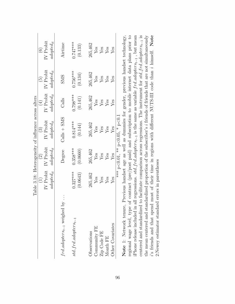
Tab

le3.

18:

Het

erog

enei

tyof

influen

ceac

ross

alte

rs(1

)(2

)(3

)(4

)(5

)(6

)IV

Pro

bit

IVP

robit

IVP

robit

IVP

robit

IVP

robit

IVP

robit

adoptedit

adoptedit

adoptedit

adoptedit

adoptedit

adoptedit

frd

adopters

t−1

wei

ghed

by

...

Deg

ree

Cal

ls+

SM

SC

alls

SM

SA

irti

me

stdfrd

adopters

t−1

0.32

7***

0.35

8***

0.81

4***

0.79

8***

0.75

6***

0.74

7***

(0.0

643)

(0.0

660)

(0.1

44)

(0.1

41)

(0.1

34)

(0.1

33)

Obse

rvat

ions

265,

462

265,

462

265,

462

265,

462

265,

462

265,

462

Com

munit

yF

EY

esY

esY

esY

esY

esY

esZ

ipC

ode

FE

Yes

Yes

Yes

Yes

Yes

Yes

Mon

thF

EY

esY

esY

esY

esY

esY

esO

ther

Cov

aria

tes

Yes

Yes

Yes

Yes

Yes

Yes

***

p<

0.01

,**

p<

0.05

,*

p<

0.1

Note

1:N

etw

ork

tenure

,P

revio

us

han

dse

tag

eas

wel

las

dum

mie

sfo

rge

nder

,pre

vio

us

han

dse

tte

chnol

ogy,

regi

onal

wag

ele

vel,

typ

eof

contr

act

(pre

/pos

tpai

d)

and

subsc

ripti

onto

mob

ile

inte

rnet

dat

apla

ns

pri

orto

iPhon

ere

leas

ein

cluded

inal

lre

gres

sion

s.stdfrd

adopters

t−1

isth

esa

me

asva

riab

lefrd

adopters

t−1

,but

mea

nce

nte

red

and

stan

dar

diz

edto

faci

lita

teco

mpar

ison

acro

ssre

gres

sion

s.T

he

inst

rum

ent

forstdfrd

adopters

t−1

isth

em

ean

cente

red

and

stan

dar

diz

edpro

por

tion

ofth

esu

bsc

rib

er’si

frie

nds

offr

iends

that

are

not

sim

ult

aneo

usl

yi’

sfr

iends

and

that

spen

dm

ost

ofth

eir

tim

ein

regi

ons

wit

hdiff

eren

tN

UT

S-I

IIco

de

than

ihim

self

.N

ote

2:N

ewey

esti

mat

orst

andar

der

rors

inpar

enth

eses

96

3.7.3 The impact of having a time varying social network

A central hypothesis of our analysis is that social ties inferred from the communication

network of the EURMO are stable over the 11 month period that we analyze. To relax

this assumption we use SIENA (Snijders et al., 2010). SIENA is an implementation of

Stochastic Actor-Based Models for the Co-evolution of Network Dynamics and Behavior

(SAMCNDB) (Snijders et al., 2010) that can be used to model the dynamics of link forma-

tion across members of a social network and the relationships between the emerging social

network structure and behavior (Snijders et al., 2010).

The Mechanics of SIENA

SIENA requires two or more snapshots of the social network and of the behavior of inter-

est. Additional individual and network characteristics that may affect tie formation and

behavior can be added to the model to increase its explanatory power. Agents play a game

that establishes a path from one snapshot to the next. At every discrete point in time,

called mini-step, one agent is selected to take action. For each actor, the time between

mini-steps is modeled as a Poisson process with a constant rate parameter λ common to all

actors. Two types of actions can occur. At a network mini-step actors create or eliminate

a tie in the social network. They do so to maximize the utility given by a network objective

function of the form fi(B, x) =∑

k BkSki(x), which is a sum over all effects k of the utility

associated with each effect, Ski(x), weighted by a scaling factor, Bk. The utility associated

with an effect depends on the state of the network, x. At a behavioral mini-step actors can

change their behavior. In the case of the diffusion of the iPhone 3G, at such a mini-step,

97

actors choose whether they want to adopt this handset. They do so to maximize the utility

given by a behavioral objective function of the form fZi (BZ , x, z) =

∑k B

ZkSki(x, z), which

is the sum over all effects k of the behavioral utility associated with each effect, SZki

(x, z),

weighted by a scaling factor, BZk

. In this case, utility depends not only on the state of the

network but also on the current behavior of all other agents, z.

Functions S and SZ represent effects that according to social network theory influence

tie formation and behavior, respectively. Examples include transitivity: friends of friends

are likely to become friends, and homophily: people who are similar and behave similarly

are likely to become friends. Borrowing from the econometric theory of random utility

models, SIENA introduces a separable unobservable in the utility function of each actor.

Such error term is assumed to follow a type one extreme value distribution with mean 0

and a scale parameter normalized to 1. As a consequence the probability with which an

actor chooses an action is characterized by a multinomial logit function. For example, at

each network mini-step the probability that action a is selected across all actions in action

space A is given by efi(B,x(a)))/∑

a∈A efi(B,x(a′))).

Parameters Bk and BZk together with the rate parameter λ, which determines the

waiting time between actors’ actions, form a vector that parameterizes the probability dis-

tribution of a Markov process that captures the dynamics of the game described above.

The likelihood function of such process is often impossible to determine analytically (Sni-

jders, 1996). For this reason, SIENA estimates the parameters using a method of moments.

The solutions for the moment equations are approximated using Monte Carlo simulation

(Snijders, 2001).

98

SIENA requires that both network and behavioral changes between consecutive snap-

shots embody enough variance to allow for estimating the parameters of interest. However,

such changes cannot be so large as to challenge the assumption that snapshots are indeed

observations of a network that is gradually changing over time (Snijders et al., 2010). For

this reason, below we detail very carefully how we prepare our sample to fit the SIENA

model.

Preparing the sample and choosing the model variables

Let [t1; t2] denote a period starting in the first day of month t1 and finishing in the last

day of month t2. For each community in the sample, we break the eleven months of

communication data that we have in two distinct and non overlapping periods that we use

to parameterize the SIENA. Several time partitions were possible. We choose to focus on

partition [1; 4] − [5; 11]. This break down of the sample provides a good balance between

the time span of each period as well as the number of adoption events in both periods

(1058 adoptions in the first snapshot and 700 adoptions in the second snapshot). Several

alternative partitions were considered and tested which did not affect the results. Appendix

3.D provides the output for all possible two-snapshot combinations.

For partition [1; 4] − [5; 11], the changes in the social network across time are small,

that is, a substantial proportion of the ties linking individuals in each of the communities

in the sample remains unchanged from the first to the second period. This is evidence that

the social network structure is rather stable and that the communication links captured

in the communication network are likely to entail real social meaning rather than sporadic

99

communication interaction.

Still, for these two periods, there are communities in our sample with little variation

in the adoption of the iPhone 3G across time. In 30 communities (out of 263) there is no

variability in adoption behavior from the first to the second period and for 80 others, there

is variation in behavior, but too little change for SIENA to converge to acceptable levels

in the behavioral part of the model.

For each community and time period, we create an adjacency matrix Act with actij > 0

indicating that user i in community c called or sent an sms to user j during time period t.

We use a vector yct to register the behavior of interest. ycti > 0 indicates that user i owned

the iPhone 3G during the time period t7. These variables are the main parameterizations

of the SIENA model.

Additionally, to explain the evolution of the social network, we include in our SIENA

model, the effect of outdegree =∑

j actij that measures the overall tendency to form ties

which are costly to establish and to maintain, reciprocity =∑

j aijaji that controls for

the fact that people tend to return calls and sms from their friends and transitivity =∑j aijmaxh(aih, ahj) to account for triad closure bias, that is, people tend to communi-

cate with the friends of their friends. We also include the effect of adoptionsimilarity =∑j aij(simij − simi) with simij = 1{yi = yj} that captures the tendency that individuals

may establish links to other individuals that display the same behavior. This effect esti-

mates homophily in the adoption of the iPhone 3g, in other words, the impact that the

adoption of the iPhone 3g will have in the structure of the social network. For ease of

7No subscriber in our sample adopted the iPhone 3G and then switched to another handset.

100

comprehension we named this effect Behavior− > Network.

To explain behavior we focus on the effect adoptionaveragesimilarity =∑

j aijsimij/∑

j aij

that controls for influence and is scaled by the size of the social circle. In this case, the

effect captures the level of exposure that each user has to the innovation. We identify this

effect by Network− > Behavior.

SIENA provides several alternative effects that allow controlling for influence and ho-

mophily. We chose the ones reported above following the recommendations in (Ripley

and Snijders, 2010) and (Snijders et al., 2010). The adoption of the iPhone is coded as

binary event and the SIENA manual recommends the utilization of covariate similarity for

controlling homophilous attachment in such cases. Finally, we chose the influence effect

adoptionaveragesimilarity because it reflects the concept of exposure (Valente, 1996b)

and it permits an interpretation that is possible to compare with the marginal effect of

peer influence that we estimate in the previous sections of the paper.

SIENA model output

We fit SIENA to each community in our sample. For the communities such that SIENA

converges, we obtain estimates for the set of parameters described above. We combine

the estimation results of the different parameters across the different communities using

meta-analysis (Hedges and Olkin, 1985; DerSimonian and Laird, 1986; Viechtbauer, 2010)

to obtain a summary effect.

We estimate the summary effect for each variable in our model through a random-

effects model to allow the true effect of each parameter to vary across communities rather

101

than impose a true value of the effect shared by all(DerSimonian and Laird, 1986). We

use a restricted maximum likelihood estimator to obtain the summary effect (Paule and

Mandel, 1982; Rukhin et al., 2000) and we use the standard error bias correction suggested

by (Knapp and Hartung, 2003)8.

For each coefficient summary effect estimate, we perform a Q-test of heterogeneity

(Huedo-Medina et al., 2006). The null hypothesis of the test assumes that the true value

of the parameter is the same across the communities included in the estimation proce-

dure(Higgins and Thompson, 2002; Huedo-Medina et al., 2006). For a given parameter, if

the null hypothesis of the Q-test is rejected, there is evidence of unobserved heterogene-

ity explaining the difference in the parameter estimates across communities that is not

attributable to sampling error. Such scenario provides an argument against reporting a

single summary effect for the set of communities. On the contrary, if the null hypothesis

of the Q-test is not rejected, we are more confident that differences in the parameter es-

timates across communities are a consequence of sampling error and the summary effect

may be interpreted as an estimator for the true parameter value in the population(Higgins

and Thompson, 2002).

To provide a more complete picture of the analysis we also report the I2 index which

measures the percentage of the total variation in effect sizes across communities that is

caused by between-studies variability (unobserved heterogeneity in our communities)(Huedo-

Medina et al., 2006).

Table 3.19 contains the results. We highlight that the effect of peer influence, measured

8Nevertheless, using other estimators such as the DerSimonian-Laird estimator, Maximum Likelihoodor Empirical Bayes yields similar results in this case

102

by the parameter Network− > Behavior is positive and statistically significant at the 1%

level. We find influence even in the presence of a changing social network over time. For

this parameter, we cannot reject the null hypothesis of the Q-test, as such the summary

effect can be interpreted population wise with respect the communities in our analysis.

Furthermore, the I2 index for this effect is essentially zero which implies that the variation

in the estimation results that occurs across communities can be attributable to sampling

error.

Behavior− > Network is positive, but not statistically significant across the commu-

nities. The Q-test provides evidence of heterogeneity across communities sampled for this

effect. Moreover I2 is large. These results do not provide sufficient proof of the role ho-

mophily may have played in the diffusion of the iPhone 3G, that is, we do not find robust

evidence that similar behavior in terms of adoption of the iPhone 3g leads to changes in

the network ties.

Figure 3.8 is a scatter plot of the 153 estimates of the coefficients of influence (top

panel) and homophily (bottom panel) together with their standard errors and statistically

significance. The picture shows that the Behavior− > Network coefficient varies signifi-

cantly across communities. In some cases, the effect of is negative and significant, in other

communities it is positive and significant. Still, for a majority of the scenarios, the effect

is close to zero and not statistically significant.

We note that for the other variables, the Q-test rejects the null hypothesis and the

corresponding I2 is large which implies that there are unobservables deriving the variation

of those parameters across the communities. Nevertheless, the coefficients obtained from

103

the meta-analysis exhibit the expected signs. This means that, on average, across the

communities we sampled, they behave as theory predicts. Random ties are not likely to

form and reciprocity and transitivity have a positive impact on tie formation.

Table 3.19: Results of the meta-analysis for each of the behavioral and network effectsincluded in the SIENA model

name coeff stderr pval I2 H2 τ2 Q-Test Q-Test N obs(p-val)

outdegree (density) -4.414 0.043 0.000 62.851 2.692 0.182 543.708 0.000 153reciprocity 4.398 0.067 0.000 75.399 4.065 0.448 782.592 0.000 153transitive ties 2.174 0.034 0.000 51.141 2.047 0.086 345.009 0.000 153

Behavior− > Network 0.043 0.044 0.334 24.219 1.320 0.061 208.778 0.002 153

Network− > Behavior 3.168 0.102 0.000 0.000 1.000 0.000 62.002 1.000 153Note 1: variable Behavior− > Network is captured by the behaviorsimilaritySIENA effect; Note 2: variable Network− > Behavior is implemented through thebehavioraveragesimiliraty SIENA effect; Note 3: Meta analysis estimated through Maxi-mum Likelihood assuming a random effects model with Knapp and Hartung standard errorcorrection; Note 4: τ2 is the estimate of total amount of heterogeneity, I2 is the % of totalvariability due to heterogeneity, H2 is totalvariability

samplingvariability .

(a) Network− > Behavior (b) Behavior− > Network

Figure 3.8: Scatter plot for the 153 estimates of the Network− > Behavior andBehavior− > Network variables of the SIENA model

104

Interpretation of the effect

In SIENA, for a behavioral mini-step of the simulator, the log-odds ratio of adoption vs.

no adoption for the Network− > Behavior is given by β(Ad − NAd)/(Ad + NAd). Ad

denotes the number of friends that adopted the iPhone 3g, NAd denotes the number of

friends that did not adopt the iPhone 3G and β denotes the coefficient of the effect9.

For a subscriber i for whom all friends j have adopted the iPhone 3g (NAd = 0),

the log-odds simplifies to β. Therefore, the odds ratio of adoption vs no adoption is

p′1−pp

1−p= exp(3.168) = 23.760 where p denotes the probability of adoption for an individual

for whom all his friends adopted and p′ denotes the probability of adoption for an individual

whom no friend adopted the handset.

A comparable figure can be computed for the probit model presented in section 3.6.

Using the model estimated in section 3.6, we estimated that the average instantaneous

probability of adoption of across the individuals that had no prior adopter friends is 0.006.

Using instrumental variables, we estimate that for a user whom all friends adopted the

iPhone 3g, the instantaneous probability of adopting would increase by 0.150 with a stan-

dard error of 0.032. Such information can be used to compute the odds ratios of having

all friends adopting the iPhone versus no friend adopting which is comparable to the odds

ratio that SIENA estimates.

At the mean of the confidence interval of the marginal effect of peer influence, the odds

ratio for the probit formulation is given byp′

1−p′p

1−p=

0.006+0.1501−(0.006+0.150)

0.0061−0.006

= 30.6. At the lower end of

the confidence interval for the marginal effect, the odds ratio isp′

1−p′p

1−p=

0.006+0.0871−(0.006+0.0087)

0.0061−0.006

= 16.9.

9Additional details can be obtained from (Ripley and Snijders, 2010, page 148)

105

This shows that magnitude of the influence effect estimated through SIENA is in the same

order of magnitude of that reported in the previous sections of the paper.

3.8 Policy Experiment

In this section we estimate whether common heuristic marketing strategies, such as those

described in (Bampo et al., 2008) and (Hinz et al., 2011) could have helped spread further

the adoption of the iPhone 3G at EURMO. For this purpose, we code a simulator that

computes the additional expected number of adopters as a function of a particular seeding

strategy. Table 3.20 presents the pseudo-code for our simulator. At the outset n seeds are

selected to adopt the iPhone 3G. The probability of adoption for each individual evolves

over time according to the adjacency matrix W for the set of users considered, S, and a

fixed exogenous marginal effect for peer influence, m. To keep our simulator sufficiently

simple we disregard influence across paths through subscribers that do not belong to S

and we assume the same marginal effect for all subscribers in S. The number of adopters

evolves according to this dynamic probability up to time T , which we set to 12 months in

our simulations. In table 3.20 A(0) = Policyk(n,m, S) instantiates the seeding policy.

Table 3.21 summarizes the seeding strategies that we investigate and figure 3.9 shows

the results we obtained. Panel (a) in this figure shows the number of additional adopters

as a function of the seeing policy and of the number of iPhone 3G awarded. The random

strategy performs the poorest and local degree yields the most additional adopters. Panel

(b) in this figure shows the cost/revenue ratio, C/R, for which each policy breaks-even.

While the random strategy could only break even if the cost to produce the iPhone 3G is

106

Table 3.20: Pseudo-code for policy simulatorKey variables

k policy indicator (0 for no policy)n number of policy seedsm marginal peer influence effectS set of subscribers

α, β, γ, ρ parameters from probit estimationW , Xi, Zit covariates in equation (6)AO(i, t) adoptions observed in our datasetA(i, t) adoptions generated in simulationBPA(i, t) baseline probability of adoptionPA(i, t) probability of adoption

Algorithm

function Simulator(k,n,m,S)TotalAA =

∑Nj=1(AA(k, n,m, S)− AA(0, 0,m, S))

return TotalAA/N − nend function

function AA(k,n,m,S) - Additional AdoptersA(0) =Policyk(n,m, S)for t = 0→ T, i ∈ S do

BPA(i, t) = Φ(α +Xiβ + γZit + ρWAO(t− 1))end forfor t = 0→ T, i ∈ S : A(i, t) == 0 do

PA(i, t) = BPA(i, t) +mW (A(t− 1)− AO(t− 1))A(i, t) = 1{draw U(0, 1) > PA(i, t)}

end forreturn

∑i∈S A(i, T )

end function

no more than 20% of the revenue, the local and global degree strategies can break even at

higher ratios. Policy k breaks even if AA(k, n,m, S)(R − C) = nC. According to iSuppli

http://www.isuppli.com/ the iPhone 3G marginal cost is roughly 50% of the revenue.

If this estimate is true panel (b) in Figure 3.9 shows that all the policies tested here can

hardly break even.

107

Table 3.21: Policy Interventions TestedPolicy t = 0 Policy DescriptionRandom Award the iPhone 3G to a random sample of n subscribers in SGlobal Degree Award the iPhone 3G to the n subscribers in S with highest degreeGlobal Between-ness

Award the iPhone 3G to the top n subscribers in S with highestbetweenness

Local Degree Randomly select n communities with replacement and at each drawaward the iPhone 3G to the subscriber with the highest degree inthat community still without one

Figure 3.10 shows a sensitivity analysis on the marginal effect of peer influence for the

case of global degree, which is the most popular seeding strategy used by firms to explore

viral marketing (Hinz et al., 2011). Panel (a) in this figure shows that this seeding strategy

can only break even if the marginal effect of peer influence is substantially higher than our

IV probit estimation. Still, panel (b) in this same figure, derived assuming C = 300

and R = 600, shows that with high levels of peer influence viral marketing strategies can

sometimes increase expected profits by as much as 50%.

3.9 Conclusion

This paper studies the effect of peer influence in the diffusion of the iPhone 3G across a

number of communities that were sampled from a large dataset from a major European

Mobile (EURMO) carrier in one country.

We use instrumental variables to control for potential correlation between unobserved

subscriber heterogeneity and peer influence. Our goal was to show whether there is a rela-

tionship between the percentage of friends who adopt the iPhone 3G and one’s propensity

to do so. We instrument the friend’s decision to adopt with the adoption decisions of

108

(a) Additional Adopters

(b) C/R for breakeven

Figure 3.9: Policy outcomes of awarding the iPhone 3G to different numbers of policytargets

109

(a) C/R for breakeven

(b) Additional profits

Figure 3.10: Potential profits from seeding the iPhone 3G with global degree

the friends of friends that are not friends of the ego that live in a different city from the

one where the ego does. This instrument explains well the adoption decisions of friends

and provides separation, both geographically and in terms of the call graph, between the

instrument and the ego. In fact, we provide several robustness checks that show that our

110

instrument behaves as expected.

We provided evidence that the propensity of a subscriber to adopt increases with the

percentage of friends that had already adopted. We estimated that 14% of iPhone 3G

adoptions in EURMO were due to peer influence, after controlling for social clustering,

gender, previous adoption of mobile internet data plans, ownership of technologically ad-

vanced handsets and some heterogeneity in the regions where subscribers move during the

day and spend most of their evenings. Our estimate for peer influence without IV is three

times lower that the above statistic, which hints that unobserved effects might be neg-

atively correlated with adoption. We provide additional empirical evidence that budget

constraints might be at work preventing several family members, or many employees in the

same company, from purchasing the iPhone 3G, which was a conspicuous and expensive

handset for the average consumer in the country studied.

We also provide results from several policy experiments that show that with an effect of

peer influence with this magnitude EURMO would hardly be able to significantly increase

sales by selectively targeting appropriate early adopters to benefit from viral marketing.

We show that a seeding strategy using local degree yields the largest number of additional

adopters among the strategies compared in this paper, but even such policy could only

hardly break even for the cost/revenue ratio at which the iPhone 3G might have been

commercialized.

Our paper also comes with limitations. On one-hand, our analysis relies on a random

sample of clusters of subscribers that call more within the cluster. We used this technique

to sample our dataset to control for unobserved con founders that could determine adoption

111

and social network ties. That is particularly important given our IV strategy that relies

on the actual structure of the social network. However, this clustering criterion is not

unique and multiple runs of our sampling algorithm could also produce slightly different

community structures.

We attempted to use other algorithms of community extraction to repeat the analysis,

but we show in this paper that the community algorithms that are able to deal with very

large networks such as our own, do not provide partitions of the data that would be useful

for the type of analysis that we conduct.

On the other hand, we use communication events as a proxy for social proximity, but

we only have access to text and voice communications. It is possible that people use other

means of communications, such as e-mail and face to face meetings, that can just as equally

spread information about the iPhone 3G and trigger or hinder adoption. However, we are

not able to control for them in our case.

Finally we only use data from EURMO but other mobile operators in the same country

also offered the iPhone 3G. Therefore, it is possible that friends that do not subscribe to

EURMO might have also played a role in shaping the diffusion of the iPhone 3G across

EURMO subscribers, but we are unable to account for them. Still in the country in

question, EURMO is a dominant player with respect to the adoption of the iPhone 3G.

Only two operators licensed agreements for this handset from day one of its release (the

other major operator in the country launched the iPhone 3G only much latter): EURMO,

whose market share is approximately 40%, and another operator, whose market share is

about 17%. Therefore, it is likely that most iPhone adoption occurred with EURMO.

112

Furthermore, the prices at which these two operators offered the iPhone 3G were similar

and thus it is hard to believe that there was disproportionately more adoption with the

other carrier. Additionally, in the country analyzed, the prices to call someone in other

networks are considerably higher than those to call within the same operator (on average

the former is 40% more expensive), therefore a majority of one’s friends belongs to the same

operator. In fact, from the data we have, on average, each month, EURMO subscribers

call seven times more other EURMO subscribers than subscribers in any other network.

Therefore, it is even more likely that one’s friends adopting the iPhone belong to the same

carrier.

113

114

References

Jeffrey A. Smith and Petra E. Todd. Does matching overcome LaLonde’s critique ofnonexperimental estimators? Journal of Econometrics, 125(1-2):305–353, 2005. ISSN03044076. doi: 10.1016/j.jeconom.2004.04.011. 3.2.2

A. Albert and J. A. Anderson. On the existence of maximum likelihood estimates in logisticregression models. Biometrika, 71(1):1–10, April 1984. ISSN 0006-3444. doi: 10.2307/2336390. URL http://www.jstor.org/stable/2336390. ArticleType: research-article/ Full publication date: Apr., 1984 / Copyright c© 1984 Biometrika Trust. 3.6

Paul D. Allison. Discrete-time methods for the analysis of event histories. SociologicalMethodology, 13:61–98, January 1982. ISSN 0081-1750. doi: 10.2307/270718. URLhttp://www.jstor.org/stable/270718. ArticleType: research-article / Full publica-tion date: 1982 / Copyright c© 1982 John Wiley & Sons. 3.5, 3.7.1

A. Anagnostopoulos, R. Kumar, and M. Mahdian. Influence and correlation in socialnetworks. pages 7–15. ACM, 2008. 3.2.2

S. Aral. Commentary–identifying social influence: A comment on opinion leadership andsocial contagion in new product diffusion. Marketing Science, 30(2):217–223, 2010. ISSN0732-2399 1526-548X. doi: 10.1287/mksc.1100.0596. 3.2.2

S. Aral, L. Muchnik, and A. Sundararajan. Distinguishing influence based contagion fromhomophily-driven diffusion in dynamic networks. Proceedings of the National Academyof Sciences, 106(51):21544, 2009. ISSN 0027-8424. 3.1, 3.2.2, 3.4

Sinan Aral. Influence or be influenced: the cause and effect of your social network.http://poptech.org/e1 sinan aral, March 2012. URL http://poptech.org/e1_sinan_

aral. 3.2.2

Sinan Aral and Dylan Walker. Creating social contagion through viral product design:A randomized trial of peer influence in networks. Management Science, 57(9):1623–1639, January 2011. ISSN 0025-1909, 1526-5501. doi: 10.1287/mnsc.1110.1421. URLhttp://mansci.journal.informs.org/content/57/9/1623. 3.2.2

Jim Bagrow and Erik Bollt. A local method for detecting communities. arXiv:cond-mat/0412482, December 2004. doi: 10.1103/PhysRevE.72.046108. URL http://arxiv.

org/abs/cond-mat/0412482. Phys. Rev. E, 72 046108 (2005). 3.1

Mauro Bampo, Michael T. Ewing, Dineli R. Mather, David Stewart, and Mark Wallace.The effects of the social structure of digital networks on viral marketing performance.Information systems research, 19(3):273–290, September 2008. ISSN 1047-7047, 1526-5536. URL http://dro.deakin.edu.au/view/DU:30017617. 3.2.2, 3.8

Ravi Bapna and Akhmed Umyarov. Do your online friends make you pay? a randomizedfield experiment in an online music social network. NBER, July 2012. URL http:

//conference.nber.org/confer/2012/SI2012/PRIT/Bapna_Umyarov.pdf. 3.2.2

Frank Bass. Bass. a new product growth for model consumer durables. ManagementScience, 15(5):215–227, 1969. 3.2.2

115

C. F. Baum, M. E. Schaffer, and S. Stillman. Enhanced routines for instrumental vari-ables/generalized method of moments estimation and testing. Stata Journal, 7(4):465,2007. 3.7.1, 5

D. Birke and P. Swann. Network effects in mobile telephony. COMPETITION ANDREGULATION, page 12, 2007. 3.1

Daniel Birke and G. M. Peter Swann. Network effects and the choice of mobile phoneoperator. Journal of Evolutionary Economics, 16(1-2):65–84, 2005. ISSN 0936-99371432-1386. doi: 10.1007/s00191-005-0001-5. 3.1

Daniel Birke and G.M. Peter Swann. Network effects, network structure and con-sumer interaction in mobile telecommunications in europe and asia. Journal of Eco-nomic Behavior & Organization, 76(2):153–167, November 2010. ISSN 0167-2681. doi:10.1016/j.jebo.2010.06.005. URL http://www.sciencedirect.com/science/article/

pii/S016726811000106X. 3.1

Vincent D Blondel, Jean-Loup Guillaume, Renaud Lambiotte, and Etienne Lefebvre.Fast unfolding of communities in large networks. Journal of Statistical Mechan-ics: Theory and Experiment, 2008(10):P10008, October 2008. ISSN 1742-5468. doi:10.1088/1742-5468/2008/10/P10008. URL http://iopscience.iop.org/1742-5468/

2008/10/P10008. (document), 3.1, 3.4.2, 3.C.5

Anabela Botelho and Lı´gia Costa Pinto. The diffusion of cellular phones in portugal.Telecommunications Policy, 28(5–6):427–437, June 2004. ISSN 0308-5961. doi: 10.1016/j.telpol.2003.11.006. URL http://www.sciencedirect.com/science/article/

pii/S0308596104000424. 3.2.2

Vincent Boucher, Yann Bramoulle, Habiba Djebbari, and Bernard Fortin. Do peers af-fect student achievement? evidence from canada using group size variation. SSRNeLibrary, January 2010. URL http://papers.ssrn.com/sol3/papers.cfm?abstract_

id=1545150. 3.1

Yann Bramoulle and Brian W. Rogers. Diversity and popularity in social networks. SSRNScholarly Paper ID 1336634, Social Science Research Network, Rochester, NY, February2009. URL http://papers.ssrn.com/abstract=1336634. 3.5

Y. Bramoulle and B. Fortin. The econometrics of social networks. CIRPEE WorkingPapers, 09-13, February 2009. 3.2.2

Yann Bramoulle, Habiba Djebbari, and Bernard Fortin. Identification of peer effectsthrough social networks. Journal of Econometrics, 150(1):41–55, 2009. ISSN 03044076.doi: 10.1016/j.jeconom.2008.12.021. 3.2.2, 3.5

Erik Brynjolfsson and Chris F. Kemerer. Network externalities in microcomputer software:An econometric analysis of the spreadsheet market. Management Science, 42(12):1627–1647, December 1996. ISSN 0025-1909. URL http://www.jstor.org/stable/2634543.ArticleType: research-article / Full publication date: Dec., 1996 / Copyright c© 1996INFORMS. 3.1

Ronald S. Burt. Formalizing the argument. In Structural Holes. Harvard University Press,

116

1980. 3.5

Ronald S. Burt. Social contagion and innovation: Cohesion versus structural equivalence.The American Journal of Sociology, 92(6):1287–1335, 1987. ISSN 00029602. 3.1, 3.2.1,3.5

Scott E. Carrell, Richard L. Fullerton, and James E. West. Does your cohort matter? mea-suring peer effects in college achievement. Journal of Labor Economics, 27(3):439–464,July 2009. ISSN 0734-306X. URL http://www.jstor.org/stable/10.1086/600143.ArticleType: research-article / Full publication date: July 2009 / Copyright c© 2009The University of Chicago. 3.1

A. Carvalho. Diffusion of mobile phones in portugal: Unexpected success. In InnovationPressure International ProACT Conference Rethinking Competitiveness, Policy and So-ciety in a Globalised Economy. Tampere, Finland, 2006. 3.2.2

Anne C. Case and Lawrence F. Katz. The company you keep: The effects of family andneighborhood on disadvantaged youths. National Bureau of Economic Research WorkingPaper Series, No. 3705, 1991. URL http://www.nber.org/papers/w3705. featured inNBER digest on 1991-07-01. 3.1

T.L. Childers and A.R. Rao. The influence of familial and peer-based reference groups onconsumer decisions. Journal of Consumer research, page 198–211, 1992. 3.1, 3.3.1

Wen-Lin Chu, Feng-Shang Wu, Kai-Sheng Kao, and David C. Yen. Diffusion of mobiletelephony: An empirical study in taiwan. Telecommunications Policy, 33(9):506–520,October 2009. ISSN 0308-5961. doi: 10.1016/j.telpol.2009.07.003. URL http://www.

sciencedirect.com/science/article/pii/S0308596109000743. 3.2.2

Aaron Clauset. Finding local community structure in networks. Physical Review E, 72(2):026132, August 2005. doi: 10.1103/PhysRevE.72.026132. URL http://link.aps.org/

doi/10.1103/PhysRevE.72.026132. 3.4.2

Aaron Clauset, M. E. J. Newman, and Cristopher Moore. Finding community structurein very large networks. Physical Review, 70(6), 2004. (document), 3.1, 3.4.2, 3.C.4

J.S. Coleman, E. Katz, H. Menzel, and Columbia University. Bureau of Applied SocialResearch. Medical innovation: A diffusion study. Bobbs-Merrill Co., 1966. 3.1

Gabor Csardi and Tamas Nepusz. iGraph reference manual. Technical report, 2005. URLhttp://igraph.sourceforge.net/doc/igraph-docs.pdf. 3, 3.C.2

Koustuv Dasgupta, Rahul Singh, Balaji Viswanathan, Dipanjan Chakraborty, SougataMukherjea, Amit A. Nanavati, and Anupam Joshi. Social ties and their relevance tochurn in mobile telecom networks. In Proceedings of the 11th international conference onExtending database technology: Advances in database technology, pages 668–677, Nantes,France, 2008. ACM. doi: 10.1145/1353343.1353424. 3.1

Rebecca DerSimonian and Nan Laird. Meta-analysis in clinical trials. ControlledClinical Trials, 7(3):177–188, September 1986. ISSN 0197-2456. doi: 10.1016/0197-2456(86)90046-2. URL http://www.sciencedirect.com/science/article/pii/

0197245686900462. 3.7.3

117

Torsten Dierkes, Martin Bichler, and Ramayya Krishnan. Estimating the effect of wordof mouth on churn and cross-buying in the mobile phone market with markov logicnetworks. Decision Support Systems, 51(3):361–371, June 2011. ISSN 0167-9236. doi:10.1016/j.dss.2011.01.002. URL http://www.sciencedirect.com/science/article/

pii/S0167923611000273. 3.1

Toker Doganoglu and Lukasz Grzybowski. Estimating network effects in mobile telephonyin germany. Information Economics and Policy, 19(1):65–79, March 2007. ISSN 0167-6245. doi: 10.1016/j.infoecopol.2006.11.001. URL http://www.sciencedirect.com/

science/article/pii/S0167624506000710. 3.2.2

L. Donetti and M. A. Munoz. Improved spectral algorithm for the detection of networkcommunities. arXiv:physics/0504059, April 2005. doi: 10.1063/1.2008598. URL http:

//arxiv.org/abs/physics/0504059. 3.1

Jordi Duch and Alex Arenas. Community detection in complex networks using extremaloptimization. Physical review E, 72(2):027104, 2005. URL http://pre.aps.org/

abstract/PRE/v72/i2/e027104. 3.1

The Economist. Nokia at the crossroads: Blazing platforms. The Economist, February2011. ISSN 0013-0613. URL http://www.economist.com/node/18114689?story_id=

18114689. 3.1

Bradley Efron. An introduction to the Bootstrap. Chapmann & Hall, London, 1993. ISBN9780412042317. 3.5

Joseph Farrell and Garth Saloner. Standardization, compatibility, and innovation. TheRAND Journal of Economics, 16(1):70–83, April 1985. ISSN 0741-6261. doi: 10.2307/2555589. URL http://www.jstor.org/stable/2555589. ArticleType: research-article/ Full publication date: Spring, 1985 / Copyright c© 1985 The RAND Corporation. 3.1

Santo Fortunato. Community detection in graphs. Physics Reports, 486(3–5):75–174,February 2010. ISSN 0370-1573. doi: 10.1016/j.physrep.2009.11.002. URL http://

www.sciencedirect.com/science/article/pii/S0370157309002841. 3.2.2, 3.4.1, 3.1

Santo Fortunato and Marc Barthelemy. Resolution limit in community detection. Proceed-ings of the National Academy of Sciences, 104(1):36–41, February 2007. ISSN 0027-8424,1091-6490. doi: 10.1073/pnas.0605965104. URL http://www.pnas.org/content/104/

1/36. 3.4.3

Santo Fortunato, Vito Latora, and Massimo Marchiori. A method to find communitystructures based on information centrality. arXiv:cond-mat/0402522, February 2004.doi: 10.1103/PhysRevE.70.056104. URL http://arxiv.org/abs/cond-mat/0402522.3.1

David Gefen and Detmar W. Straub. Gender differences in the perception and use ofe-mail: An extension to the technology acceptance model. MIS Quarterly, 21(4):389–400, December 1997. ISSN 0276-7783. doi: 10.2307/249720. URL http://www.jstor.

org/stable/249720. ArticleType: research-article / Full publication date: Dec., 1997/ Copyright c© 1997 Management Information Systems Research Center, University ofMinnesota. 3.5

118

M. Girvan and M.E.J. Newman. Community structure in social and biological networks.Proceedings of the National Academy of Sciences of the United States of America, 99(12):7821, 2002. 3.1

J. Goldenberg, S. Han, D.R. Lehmann, and J.W. Hong. The role of hubs in the adoptionprocess. Journal of Marketing, 73(2):1–13, 2009. ISSN 0022-2429. 3.2.2

M. Granovetter and R. Soong. Threshold models of diversity: Chinese restaurants,residential segregation, and the spiral of silence. Sociological Methodology, 18(6):69–104, 1988. URL http://www.stanfordu.edu/dept/soc/people/mgranovetter/

documents/granchineserestaurants_000.pdf. 3.2.2

Mark Granovetter. Threshold models of collective behavior. American Journal of Sociology,83(6):1420–1443, May 1978. ISSN 0002-9602. URL http://www.jstor.org/stable/

2778111. ArticleType: research-article / Full publication date: May, 1978 / Copyrightc© 1978 The University of Chicago Press. 3.2.2

Mark Granovetter and Roland Soong. Threshold models of diffusion and collective be-havior. The Journal of Mathematical Sociology, 9(3):165–179, 1983. ISSN 0022-250X.doi: 10.1080/0022250X.1983.9989941. URL http://www.tandfonline.com/doi/abs/

10.1080/0022250X.1983.9989941. 3.2.2

Mark Granovetter and Roland Soong. Threshold models of interpersonal effects in con-sumer demand. Journal of Economic Behavior & Organization, 7(1):83–99, March1986. ISSN 0167-2681. doi: 10.1016/0167-2681(86)90023-5. URL http://www.

sciencedirect.com/science/article/pii/0167268186900235. 3.2.2

M.S. Granovetter. The strength of weak ties. American Journal of Sociology, pages 1360–1380, 1973. ISSN 0002-9602. 3.2.2

Harald Gruber. Competition and innovation: The diffusion of mobile telecommuni-cations in central and eastern europe. Information Economics and Policy, 13(1):19–34, March 2001. ISSN 0167-6245. doi: 10.1016/S0167-6245(00)00028-7. URLhttp://www.sciencedirect.com/science/article/pii/S0167624500000287. 3.2.2

Il-Horn Hann, Kai-Lung Hui, Sang-Yong T. Lee, and Ivan P. L. Png. Consumer privacy andmarketing avoidance: A static model. Management Science, 54(6):1094–1103, January2008. ISSN 0025-1909, 1526-5501. doi: 10.1287/mnsc.1070.0837. URL http://mansci.

journal.informs.org/content/54/6/1094. 3.2.2

Larry V. Hedges and Ingram Olkin. Statistical Methods for Meta-Analysis. AcademicPress, 1 edition, August 1985. ISBN 0123363802. 3.1, 3.7.3

Peter Hedstrom. Contagious collectivities: On the spatial diffusion of swedish trade unions,1890-1940. American Journal of Sociology, 99(5):1157–1179, March 1994. ISSN 0002-9602. URL http://www.jstor.org/stable/2781146. 3.1

Julian P. T. Higgins and Simon G. Thompson. Quantifying heterogeneity in a meta-analysis. Statistics in Medicine, 21(11):1539–1558, 2002. ISSN 1097-0258. doi:10.1002/sim.1186. URL http://onlinelibrary.wiley.com/doi/10.1002/sim.1186/

abstract. 3.7.3

119

Shawndra Hill, Foster Provost, and Chris Volinsky. Network-based marketing: Identifyinglikely adopters via consumer networks. Statistical Science, 21(2):256–276, 2006. ISSN0883-4237. doi: 10.1214/088342306000000222. 3.2.2

O. Hinz, B. Skiera, C. Barrot, and J. U. Becker. Seeding strategies for viral marketing:An empirical comparison. Journal of Marketing, 75(6):55–71, 2011. 3.2.2, 3.8, 3.8

Tania B. Huedo-Medina, Julio Sanchez-Meca, Fulgencio Marın-Martınez, and Juan Botella.Assessing heterogeneity in meta-analysis: Q statistic or i2 index? Psychological Methods,11(2):193–206, 2006. ISSN 1939-1463, 1082-989X. doi: 10.1037/1082-989X.11.2.193.URL http://doi.apa.org/getdoi.cfm?doi=10.1037/1082-989X.11.2.193. 3.7.3

Elena Karahanna, Ritu Agarwal, and Corey M. Angst. Reconceptualizing compatibilitybeliefs in technology acceptance research. MIS Quarterly, 30(4):781–804, December2006. ISSN 0276-7783. URL http://www.jstor.org/stable/25148754. ArticleType:research-article / Full publication date: Dec., 2006 / Copyright c© 2006 ManagementInformation Systems Research Center, University of Minnesota. 3.5

E. Katz and P.F. Lazarsfeld. Personal influence: the part played by people in the flow ofmass communications. 1955. 3.2.1

Michael L. Katz and Carl Shapiro. Technology adoption in the presence of network ex-ternalities. Journal of Political Economy, 94(4):822–841, 1986. ISSN 0022-3808. URLhttp://www.jstor.org/stable/1833204. ArticleType: research-article / Full publica-tion date: Aug., 1986 / Copyright c© 1986 The University of Chicago Press. 3.1

Michael L. Katz and Carl Shapiro. Systems competition and network effects. The Journalof Economic Perspectives, 8(2):93–115, 1994. ISSN 08953309. URL http://www.jstor.

org/stable/2138538. 3.2.1

Guido Knapp and Joachim Hartung. Improved tests for a random effects meta-regressionwith a single covariate. Statistics in Medicine, 22:2693–2710, September 2003. ISSN0277-6715, 1097-0258. doi: 10.1002/sim.1482. URL http://doi.wiley.com/10.1002/

sim.1482. 3.7.3

David Krackhardt and Robert N. Stern. Informal networks and organizational crises:An experimental simulation. Social Psychology Quarterly, 51(2):123–140, 1988. ISSN01902725. 3.4.3, 3.4.3

Andrea Lancichinetti and Santo Fortunato. Community detection algorithms: A compara-tive analysis. Physical Review E, 80(5):056117, November 2009. doi: 10.1103/PhysRevE.80.056117. URL http://link.aps.org/doi/10.1103/PhysRevE.80.056117. 3.4.1

Andrea Lancichinetti, Santo Fortunato, and Filippo Radicchi. Benchmark graphs fortesting community detection algorithms. Physical Review E, 78(4):046110, October2008. doi: 10.1103/PhysRevE.78.046110. URL http://link.aps.org/doi/10.1103/

PhysRevE.78.046110. 3.4.1

Joseph Lau, Elliott M Antman, Jeanette Jimenez-Silva, Bruce Kupelnick, FrederickMosteller, and Thomas C Chalmers. Cumulative meta-analysis of therapeutic trials formyocardial infarction. New England Journal of Medicine, 327(4):248–254, 1992. 3.D.1

120

L. Lee. Identification and estimation of econometric models with group interactions, con-textual factors and fixed effects. Journal of Econometrics, 140(2):333–374, 2007. ISSN03044076. doi: 10.1016/j.jeconom.2006.07.001. 3.2.2

Lung[U+2010]fei Lee, Xiaodong Liu, and Xu Lin. Specification and estimation ofsocial interaction models with network structures. The Econometrics Journal, 13(2):145–176, July 2010. ISSN 1368-423X. doi: 10.1111/j.1368-423X.2010.00310.x.URL http://onlinelibrary.wiley.com/doi/10.1111/j.1368-423X.2010.00310.x/

abstract. 3.2.2

Roger Th A. J. Leenders. Modeling social influence through network autocorrelation:constructing the weight matrix. Social Networks, 24(1):21–47, 2002. ISSN 0378-8733.doi: Doi:10.1016/s0378-8733(01)00049-1. 3.2.1, 3.4, 3.7.2

J.P. LeSage. An introduction to spatial econometrics. Revue d’Economie industrielle,(123):19–44, 2008. ISSN 1773-0198. 3.5

Jure Leskovec, Lada A. Adamic, and Bernardo A. Huberman. The dynamics of viralmarketing. ACM Trans. Web, 1(1), May 2007. ISSN 1559-1131. doi: 10.1145/1232722.1232727. URL http://doi.acm.org/10.1145/1232722.1232727. 3.2.2

Jure Leskovec, Kevin J. Lang, Anirban Dasgupta, and Michael W. Mahoney. Commu-nity structure in large networks: Natural cluster sizes and the absence of large well-defined clusters. Internet Mathematics, 6(1):29–123, 2009. ISSN 1542-7951. doi:10.1080/15427951.2009.10129177. URL http://www.tandfonline.com/doi/abs/10.

1080/15427951.2009.10129177. 3.4.1, 3.4.2

Xu Lin. Identifying peer effects in student academic achievement by spatial autoregressivemodels with group unobservables. Journal of Labor Economics, 28(4):825–860, October2010. ISSN 0734-306X. URL http://www.jstor.org/stable/10.1086/653506. Ar-ticleType: research-article / Full publication date: October 2010 / Copyright c© 2010The University of Chicago. 3.2.2

Liye Ma, Ramayya Krishnan, and Alan Montgomery. Homophily or influence? an empiricalanalysis of purchase within a social network. 2010. URL http://community.mis.

temple.edu/seminars/files/2011/02/krishnan-homophily-influence.pdf. 3.1

V. Mahajan. Models for innovation diffusion. Sage Publications, Inc, 1985. ISBN0803921365. 48. 3.2.1, 3.2.2

Vijay Mahajan, Eitan Muller, and Frank M. Bass. New product diffusion models in mar-keting: A review and directions for research. Journal of Marketing, 54(1):1–26, January1990. ISSN 0022-2429. doi: 10.2307/1252170. URL http://www.jstor.org/stable/

1252170. ArticleType: research-article / Full publication date: Jan., 1990 / Copyrightc© 1990 American Marketing Association. 3.2.2

Charles F. Manski. Identification of endogenous social effects: The reflection problem. TheReview of Economic Studies, 60(3):531–542, 1993. 3.1, 3.2.2, 3.5

marketsandmarkets.com. Mobile phone & smartphone market globalforecast (2010-2015), market research report: MarketsandMarkets.

121

http://www.marketsandmarkets.com/Market-Reports/smartphone-market-219.html,February 2011. URL http://www.marketsandmarkets.com/Market-Reports/

smartphone-market-219.html. 3.1

M. McPherson, L. Smith-Lovin, and J.M. Cook. Birds of a feather: Homophily in socialnetworks. Annual review of sociology, pages 415–444, 2001. ISSN 0360-0572. 3.1, 3.2.2,3.5, 3.5

H. Menzel. Innovation, integration, and marginality: a survey of physicians. AmericanSociological Review, pages 704–713, 1960. ISSN 0003-1224. 3.2.1

L. Mercken, T.A.B. Snijders, C. Steglich, E. Vartiainen, and H. de Vries. Dynam-ics of adolescent friendship networks and smoking behavior. Social Networks, 32(1):72–81, January 2010. ISSN 03788733. doi: 10.1016/j.socnet.2009.02.005. URLhttp://linkinghub.elsevier.com/retrieve/pii/S0378873309000082. 3.1

Vision Mobile. Mobile platforms: The clash of ecosystems. Technical report, Vision Mobile,November 2011. 3.1

M. E. J Newman. Fast algorithm for detecting community structure in networks.arXiv:cond-mat/0309508, September 2003. doi: 10.1103/PhysRevE.69.066133. URLhttp://arxiv.org/abs/cond-mat/0309508. Phys. Rev. E 69, 066133 (2004). 3.1, 3.C.4

Mark EJ Newman and Michelle Girvan. Finding and evaluating community structure innetworks. Physical review E, 69(2):026113, 2004. URL http://pre.aps.org/abstract/

PRE/v69/i2/e026113. 3.1, 3.4.3

M.E.J. Newman. Detecting community structure in networks. The European PhysicalJournal B-Condensed Matter and Complex Systems, 38(2):321–330, 2004. ISSN 1434-6028. 3.2.2, 3.4

Gal Oestreicher-Singer and Arun Sundararajan. The visible hand of peer networks inelectronic markets, 2010. 3.2.2

Gergely Palla, Imre Derenyi, Illes Farkas, and Tamas Vicsek. Uncovering the overlap-ping community structure of complex networks in nature and society. Nature, 435(7043):814–818, 2005. URL http://www.nature.com/nature/journal/v435/n7043/

abs/nature03607.html. 3.1

Yousin Park and M. Ueda. A comparative study on the diffusion of smartphones in koreaand japan. In 2011 IEEE/IPSJ 11th International Symposium on Applications andthe Internet (SAINT), pages 545–549. IEEE, July 2011. ISBN 978-1-4577-0531-1. doi:10.1109/SAINT.2011.101. 3.2.2

Robert C. Paule and John Mandel. Consensus values and weighting fac-tors. Journal of Research of the National Bureau of Standards, 87(5):377–385, 1982. URL http://www.waduicenter.com/toolbox/documents/

Exhibit147ConsensusValuesandWeightingFactorsPauleandMandel-1982.pdf.3.7.3

Pascal Pons and Matthieu Latapy. Computing communities in large networks us-ing random walks. Journal of Graph Algorithms and Applications, 10(2):191–218,

122

2006. URL http://arxiv.org/PS_cache/physics/pdf/0512/0512106v1.pdfhttp:

//www.cs.brown.edu/sites/jgaa/accepted/2006/PonsLatapy2006.10.2.pdfhttp:

//www-rp.lip6.fr/~latapy/Publis/communities.pdf. (document), 3.4.1, 3.1, 3.4.2,3.C.2

Filippo Radicchi, Claudio Castellano, Federico Cecconi, Vittorio Loreto, and DomenicoParisi. Defining and identifying communities in networks. Proceedings of the NationalAcademy of Sciences of the United States of America, 101(9):2658–2663, 2004. URLhttp://www.pnas.org/content/101/9/2658.short. 3.1

Usha Nandini Raghavan, Reka Albert, and Soundar Kumara. Near linear time algorithm todetect community structures in large-scale networks. arXiv:0709.2938, September 2007.doi: 10.1103/PhysRevE.76.036106. URL http://arxiv.org/abs/0709.2938. PhysicalReview E 76, 036106 (2007). (document), 3.1, 3, 3.C.3

Neel Rao, Markus M. Mobius, and Tanya Rosenblat. Social networks and vaccination deci-sions. SSRN eLibrary, November 2007. URL http://papers.ssrn.com/sol3/papers.

cfm?abstract_id=1073143. 3.1

R.M. Ripley and T.A.B. Snijders. Manual for SIENA version 4.0. University of Oxford,Department of Statistics & Nuffield College, 2010. 3.2.2, 3.7.3, 9

E.M. Rogers. Diffusion of innovations. Free Pr, 1995. ISBN 0029266718. 3.2.2

Jeffrey Rohlfs. A theory of interdependent demand for a communications service. TheBell Journal of Economics and Management Science, 5(1):16–37, April 1974. ISSN0005-8556. doi: 10.2307/3003090. URL http://www.jstor.org/stable/3003090. Ar-ticleType: research-article / Full publication date: Spring, 1974 / Copyright c© 1974RAND Corporation. 3.1

D Romer, M Black, I Ricardo, S Feigelman, L Kaljee, J Galbraith, R Nesbit, R C Hornik,and B Stanton. Social influences on the sexual behavior of youth at risk for HIV exposure.American Journal of Public Health, 84(6):977–985, June 1994. ISSN 0090-0036, 1541-0048. doi: 10.2105/AJPH.84.6.977. URL http://ajph.aphapublications.org/doi/

abs/10.2105/AJPH.84.6.977. 3.1

M. Rosvall, D. Axelsson, and C. T. Bergstrom. The map equation. The EuropeanPhysical Journal Special Topics, 178(1):13–23, November 2009. ISSN 1951-6355, 1951-6401. doi: 10.1140/epjst/e2010-01179-1. URL http://link.springer.com/article/

10.1140/epjst/e2010-01179-1. 3.C.6

Martin Rosvall and Carl T. Bergstrom. Maps of random walks on complex networks revealcommunity structure. Proceedings of the National Academy of Sciences, 105(4):1118–1123, January 2008. ISSN 0027-8424, 1091-6490. doi: 10.1073/pnas.0706851105. URLhttp://www.pnas.org/content/105/4/1118. (document), 3.1, 3.4.2, 3.C.6

Donald B. Rubin. Matching to remove bias in observational studies. Biometrics, 29(1):159–183, 1973. ISSN 0006341X. 3.2.2

Andrew L. Rukhin, Brad J. Biggerstaff, and Mark G. Vangel. Restricted maximumlikelihood estimation of a common mean and the Mandel–Paule algorithm. Journal

123

of Statistical Planning and Inference, 83(2):319–330, February 2000. ISSN 0378-3758.doi: 10.1016/S0378-3758(99)00098-1. URL http://www.sciencedirect.com/science/

article/pii/S0378375899000981. 3.7.3

Bruce Sacerdote. Peer effects with random assignment: Results for dartmouth roommates.The Quarterly Journal of Economics, 116(2):681–704, January 2001. ISSN 0033-5533,1531-4650. doi: 10.1162/00335530151144131. URL http://qje.oxfordjournals.org/

content/116/2/681. 3.1, 3.2.2

Garth Saloner and Andrea Shepard. Adoption of technologies with network effects: Anempirical examination of the adoption of automated teller machines. The RAND Journalof Economics, 26(3):479–501, October 1995. ISSN 0741-6261. doi: 10.2307/2555999.URL http://www.jstor.org/stable/2555999. ArticleType: research-article / Fullpublication date: Autumn, 1995 / Copyright c© 1995 The RAND Corporation. 3.1

C.R. Shalizi and A.C. Thomas. Homophily and contagion are generically confounded inobservational social network studies. Sociological Methods & Research, 40(2):211, 2011.ISSN 0049-1241. 3.1, 3.2.2, 3.4, 3.5

Sanjay Kumar Singh. The diffusion of mobile phones in india. Telecommunica-tions Policy, 32(9–10):642–651, October 2008. ISSN 0308-5961. doi: 10.1016/j.telpol.2008.07.005. URL http://www.sciencedirect.com/science/article/pii/

S0308596108000773. 3.2.2

Wendell R. Smith. Product differentiation and market segmentation as alternativemarketing strategies. Journal of Marketing, 21(1):3–8, July 1956. ISSN 0022-2429.doi: 10.2307/1247695. URL http://www.jstor.org/stable/1247695. ArticleType:research-article / Full publication date: Jul., 1956 / Copyright c© 1956 American Mar-keting Association. 3.4

T. A.B Snijders. Stochastic actor-oriented models for network change. Journal of math-ematical sociology, 21(1-2):149–172, 1996. URL http://www.tandfonline.com/doi/

abs/10.1080/0022250X.1996.9990178. 3.7.3

T. A.B Snijders. The statistical evaluation of social network dynamics. Sociological method-ology, 31(1):361–395, 2001. URL http://onlinelibrary.wiley.com/doi/10.1111/

0081-1750.00099/abstract. 3.7.3

Tom A.B. Snijders, Gerhard G. van de Bunt, and Christian E.G. Steglich. Introduc-tion to stochastic actor-based models for network dynamics. Social Networks, 32(1):44–60, January 2010. ISSN 03788733. doi: 10.1016/j.socnet.2009.02.004. URL http:

//linkinghub.elsevier.com/retrieve/pii/S0378873309000069. 3.1, 3.2.2, 3.7.3,3.7.3, 3.7.3

Douglas Staiger and James H. Stock. Instrumental variables regression with weak instru-ments. Econometrica, 65(3):557–586, May 1997. ISSN 0012-9682. doi: 10.2307/2171753.URL http://www.jstor.org/stable/2171753. ArticleType: research-article / Fullpublication date: May, 1997 / Copyright c© 1997 The Econometric Society. 5

C. Steglich, T.A.B. Snijders, and M. Pearson. Dynamic networks and behavior: Separatingselection from influence. Sociological Methodology, 2010. ISSN 1467-9531. 3.2.2

124

J. H. Stock and M. Yogo. Testing for weak instruments in linear IV regression. Technicalreport, National Bureau of Economic Research, 2002. 3.7.1

David Strang. Adding social structure to diffusion models. Sociological Methods & Re-search, 19(3):324, 1991. ISSN 0049-1241. 3.2.1

David Strang and S.A. Soule. Diffusion in organizations and social movements: Fromhybrid corn to poison pills. Annual review of sociology, pages 265–290, 1998. ISSN0360-0572. 3.2.1, 3.5

David Strang and Nancy Brandon Tuma. Spatial and temporal heterogeneity in diffusion.American Journal of Sociology, 99(3):614–639, 1993. ISSN 00029602. 3.1

Taede Tillema, Martin Dijst, and Tim Schwanen. Face-to-face and electronic com-munications in maintaining social networks: the influence of geographical and rela-tional distance and of information content. New Media & Society, 12(6):965–983,January 2010. ISSN 1461-4448, 1461-7315. doi: 10.1177/1461444809353011. URLhttp://nms.sagepub.com/content/12/6/965. 3.5

C. Tucker. Identifying formal and informal influence in technology adoption with networkexternalities. Management Science, 54(12):2024–2038, September 2008. ISSN 0025-1909,1526-5501. doi: 10.1287/mnsc.1080.0897. 3.1, 3.2.2, 3.5

T.W. Valente. Network models of the diffusion of innovations. Computational & Mathe-matical Organization Theory, 2(2):163–164, 1996a. ISSN 1381-298X. 3.1, 3.2.1, 3.2.2

T.W. Valente. Social network thresholds in the diffusion of innovations. Social Networks,18(1):69–89, 1996b. ISSN 0378-8733. 3.7.3

C. Van den Bulte and G.L. Lilien. Medical innovation revisited: Social contagion versusmarketing effort. ajs, 106(5):1409–35, 2001. 3.2.1

Viswanath Venkatesh and Michael G. Morris. Why don’t men ever stop to ask for direc-tions? gender, social influence, and their role in technology acceptance and usage behav-ior. MIS Quarterly, 24(1):115–139, March 2000. ISSN 0276-7783. doi: 10.2307/3250981.URL http://www.jstor.org/stable/3250981. ArticleType: research-article / Fullpublication date: Mar., 2000 / Copyright c© 2000 Management Information SystemsResearch Center, University of Minnesota. 3.5

Viswanath Venkatesh, Michael G. Morris, Gordon B. Davis, and Fred D. Davis. User accep-tance of information technology: Toward a unified view. MIS Quarterly, 27(3):425–478,2003. ISSN 0276-7783. URL http://www.jstor.org/stable/30036540. ArticleType:research-article / Full publication date: Sep., 2003 / Copyright c© 2003 ManagementInformation Systems Research Center, University of Minnesota. 3.5

W. Viechtbauer. Conducting meta-analyses in r with the metafor package. Journal ofStatistical Software, 2010. 3.7.3

Wolfgang Viechtbauer and Mike W.-L. Cheung. Outlier and influence diagnostics for meta-analysis. Research Synthesis Methods, 1(2):112–125, 2010. ISSN 1759-2887. doi: 10.1002/jrsm.11. URL http://onlinelibrary.wiley.com/doi/10.1002/jrsm.11/abstract.3.D.1

125

Joe H. Ward. Hierarchical grouping to optimize an objective function. Journal ofthe American Statistical Association, 58(301):236–244, March 1963. ISSN 0162-1459.doi: 10.2307/2282967. URL http://www.jstor.org/stable/2282967. ArticleType:research-article / Full publication date: Mar., 1963 / Copyright c© 1963 American Sta-tistical Association. 3.C.2

Stanley Wasserman and Katherine Faust. Dynamic Network Analysis: Methods and Ap-plications. Cambridge University Press, 1994. ISBN ISBN 0-521-38707-8 Paperback.3.2.2

D. J Watts, J. Peretti, and Harvard Business School. Viral marketing for the real world.Harvard Business School Pub., 2007. 3.2.2

Duncan J. Watts. The ”New” science of networks. Annual Review of Sociology, 30:243–270, January 2004. ISSN 0360-0572. doi: 10.2307/29737693. URL http://www.jstor.

org/stable/29737693. ArticleType: research-article / Full publication date: 2004 /Copyright c© 2004 Annual Reviews. 3.2.2

Jeffrey Wooldridge and Guido Imbens. What is new in econometrics?, 2007. URL http:

//www.nber.org/minicourse3.html. 3.6

J.M. Wooldridge. Econometric analysis of cross section and panel data. The MIT press,2002. ISBN 0262232197. 3.5, 3.6, 3.13, 3.7.1

Fang Wu and Bernardo A. Huberman. Finding communities in linear time: a physicsapproach. The European Physical Journal B-Condensed Matter and Complex Systems, 38(2):331–338, 2004. URL http://www.springerlink.com/index/H6JFB70VQXADYDRM.

pdf. 3.1, 3

Bin Zhang and David Krackhardt. Extracting sub-populations from large social networks,2011. URL http://www.ml.cmu.edu/current_students/DAP_BZhang.pdf. (docu-ment), 3.1, 3.4.3, 3.C.1

Kai Zheng, Rema Padrnan, David Krackhardt, Michael PJohnson, and Herbert S Diamond.Social networks and physician adoption of electronic health records: insights from anempirical study. Journal of the American Medical Informatics, 2010. doi: 10.1136/jamia.2009.000877. 3.1

Haijun Zhou and Reinhard Lipowsky. Network brownian motion: A new method to mea-sure vertex-vertex proximity and to identify communities and subcommunities. Compu-tational Science-ICCS 2004, page 1062–1069, 2004. URL http://www.springerlink.

com/index/gq9ta1yj6eagw22e.pdf. 3.1

126

3.A Full Regression Results

Table 3.22 provides the details for the regression equation presented earlier in table 3.12

and table 3.23 details LPM alternatives that were presented in section 3.7.

Table 3.22: Complete output for the model presented in table 3.12(1) (3) (4)

Probit Probit IV ProbitVariables adoptedt adoptedt adoptedt

frd adopterst−1 3.240*** 2.851*** 9.935***(0.269) (0.258) (1.952)

[2.087]Log(tenuret + 1) 0.350*** 0.300*** 0.329***

(0.0975) (0.101) (0.0955)[0.103]

Log(tenuret + 1)2 -0.0407*** -0.0330** -0.0370***(0.0131) (0.0138) (0.0127)

[0.0139]prepaidY -0.444*** -0.549*** -0.508***

(0.0250) (0.0283) (0.0274)[0.0307]

genderF -0.0427 -0.0616* -0.0572(0.0339) (0.0343) (0.0332)

[0.0351]genderM 0.151*** 0.144*** 0.143***

(0.0250) (0.0271) (0.0261)[0.0275]

mobileNetY 0.449*** 0.425*** 0.398***(0.0434) (0.0427) (0.0397)

[0.0445]phone2.5g 0.511*** 0.484*** 0.469***

(0.0525) (0.0547) (0.0536)[0.0581]

phone3.0g 0.667*** 0.637*** 0.628***(0.0516) (0.0542) (0.0537)

[0.0596]phone3.5g 0.930*** 0.917*** 0.876***

(0.0631) (0.0658) (0.0640)[0.0735]

phoneOther 0.521*** 0.575*** 0.503***(0.138) (0.142) (0.140)

[0.162]phoneAge -0.197*** -0.143*** -0.152***

(0.0527) (0.0551) (0.0512)[0.0601]

phoneAge2 0.0413* 0.0256 0.0279(0.0240) (0.0251) (0.0240)

[0.0273]geoWageH 0.0940*** 0.133*** 0.113***

(0.0317) (0.0431) (0.0381)[0.0420]

geoWageL -0.0259 -0.146 -0.111(0.126) (0.142) (0.150)

[0.150]geoWageV H 0.117*** 0.198*** 0.150***

(0.0397) (0.0563) (0.0510)[0.0540]

Constant -3.234*** -3.602*** -3.652***(0.189) (0.214) (0.310)

[0.249]

Observations 265,462 265,462 265,462Community FE No Yes YesZip Code FE No Yes YesMonth FE Yes Yes YesPseudo R2 0.112 0.157Log Lik -9192 -8721

*** p<0.01, ** p<0.05, * p<0.1Note 1:Community clusters robust standard errors in () forProbit Note 2:Newey estimator standard errors in () for IVProbit Note 3:Community block-bootstrap standard errorsin [] for IV Probit based on 200 replications

The sign of the controls is consistent with what one would expect prior to running the

127

Table 3.23: Complete output for the model presented in table 3.15(1) (2) (3) (4)OlS OlS OlS 2SLS

VARIABLES adoptedt adoptedt adoptedt adoptedt

frd adopterst−1 0.0713*** 0.0701*** 0.0576*** 0.129***(0.00745) (0.00736) (0.00687) (0.0288)

Log(tenure+ 1) 0.00609*** 0.00576*** 0.00469** 0.00501***(0.00173) (0.00174) (0.00182) (0.00180)

Log(tenure+ 1)2 -0.000676*** -0.000636*** -0.000468* -0.000512**(0.000239) (0.000241) (0.000252) (0.000248)

prepaidY -0.00719*** -0.00726*** -0.00857*** -0.00815***(0.000540) (0.000539) (0.000618) (0.000624)

genderF -0.000510 -0.000528 -0.000644 -0.000599(0.000381) (0.000377) (0.000400) (0.000396)

genderM 0.00204*** 0.00200*** 0.00195*** 0.00195***(0.000464) (0.000462) (0.000496) (0.000493)

mobileNetY 0.0272*** 0.0271*** 0.0266*** 0.0263***(0.00404) (0.00401) (0.00388) (0.00387)

phone2.5g 0.00313*** 0.00313*** 0.00263*** 0.00247***(0.000313) (0.000311) (0.000290) (0.000310)

phone3.0g 0.00582*** 0.00578*** 0.00492*** 0.00483***(0.000404) (0.000406) (0.000394) (0.000406)

phone3.5g 0.0191*** 0.0191*** 0.0183*** 0.0179***(0.00211) (0.00211) (0.00203) (0.00201)

phoneOther 0.00256 0.00267 0.00294 0.00221(0.00257) (0.00257) (0.00256) (0.00260)

phoneAge -0.00334*** -0.00326*** -0.00195** -0.00206**(0.000893) (0.000888) (0.000907) (0.000911)

phoneAge2 0.000850** 0.000834** 0.000458 0.000486(0.000371) (0.000369) (0.000375) (0.000378)

geoWageH 0.00147*** 0.00144*** 0.00166*** 0.00145***(0.000442) (0.000547) (0.000558) (0.000558)

geoWageL 7.56e-05 -0.000554 -0.00151 -0.00117(0.00120) (0.00146) (0.00134) (0.00129)

geoWageV H 0.00207*** 0.00228** 0.00258*** 0.00211**(0.000671) (0.000895) (0.000855) (0.000849)

Constant 0.00300 0.00782 0.00680 0.0316**(0.00302) (0.00902) (0.0132) (0.0134)

Observations 265,462 265,462 265,462 265,462R-squared 0.011 0.011 0.015 0.015Community FE No No Yes YesZip Code FE No Yes Yes YesMonth FE Yes Yes Yes Yes

Community clustered standard errors in parentheses*** p<0.01, ** p<0.05, * p<0.1

128

model. This is true both before and after instrumentation.

People with previous plans of mobile internet were more likely to adopt the iPhone 3g

and the same was true for subscribers using handsets superior to 2g technology prior to

the iPhone release.

EURMO subscribers that spent most of their day time in regions with very high or high

average wage levels were more likely to adopt than individuals spending most of their time

in regions with wages close to the national average. The opposite was true for subscribers

moving in low and very low wage regions, the latter perfectly predicting non-adoption and

as such dropped from the binary outcome model.

Users subscribing to prepaid tariff plans before the iPhone release were less likely to

adopt which is as expected. The explanation is one of price since in order to buy the

iPhone 3g and still remain a prepaid subscriber, consumers needed to pay the full price

of the handset upfront. The alternative would be to change their status from prepaid to

postpaid, but in this country, consumers have a clear preference towards prepaid plans

which is also true in the EURMO operator where approximately 80% of all subscribers are

prepaid.

Finally, up to a point, network tenure was a positive contribution to the probability of

iPhone adoption even beyond the age of the handset used prior to the iPhone release. This

probably implies that subscribers required some experience with the services provided by

the EURMO prior to purchasing a phone that would bind them for at least 24 month 10.

10As mentioned in 3.3.1 all iPhone 3g handsets were sold locked to a particular the mobile communica-tions provider regardless of the nature of the contract binding the subscriber to the operator

129

3.B Instrumental Variable Details

To construct our instrumental variable ffnfdc adopterst−1 we use the social network built

from the communication graph which we have described in section 3.3, but also information

that allows us to track the regions where subscribers spend most of their time.

For each call placed or received, our dataset contains information detailing the cellular

towers that were used in the beginning of the call. Additionally, each cellular tower is

associated with GPS coordinates.

For every subscriber and for every call placed or received, we use the GPS coordinates

of the call to determine a NUTS-III regional identifier for the caller and the callee. We then

use the mode of the NUTS-III territories as the primary location of the individual since

that is the region where the subscriber was seen most often11. On average each subscriber

primary NUTS-III was identified through the analysis of 753.2 (median=387) calls.

NUTS codes - “Nomenclature of territorial units for statistics” - are statistical divisions

of the economic territory of the EU designed for developing consistent regional statistics

across EU countries and also to develop socio-economic analyses of the regions http:

//epp.eurostat.ec.europa.eu/. We choose to use NUTS-III as the unit of territorial

partitioning because by construction, these regions represent contiguous municipalities that

face the same type of economic and development challenges and within which it is likely

that people could have substantial mobility.

We only know the location of a subscriber when she performs or receives a call and

11Cell tower ranges can cover from 1 up to 30 Km therefore there is some uncertainty associated with thetrue location of each individual, particular in regions with low population density where there are fewercell towers with broader ranges.

130

by using a territorial portioning based on NUTS-III code we attempt to ensure that the

region is large enough so that each subscribers moves within rather than between most of

the time, but also we try to capture the fact that the socio-economic challenges faced by

subscribers within the same territory are similar.

Figure 3.11 depicts the number of NUTS-III codes where each subscriber was seen

receiving or placing calls.

Figure 3.11: Number of NUTS-III codes where subscribers received or placed calls fromAugust 2008 until July 2009

The average number of NUTS-III per subscriber, for the entire population of sub-

scribers, was 5.9 with a standard deviation of 4.5. Still about 25% of the subscribers were

seen placing or receiving calls within a single NUTS-III region. iPhone 3g adopters were

more mobile than the average user with an average of 10.4 NUTS-III per subscriber and a

standard deviation of 5.6. This fact does not affect our separation strategy because look-

ing in detail to the number of calls that allowed identifying each subscriber within each

NUTS-III, an overwhelming majority of calls were placed or received within the primary

NUTS-III region. This is true both overall and for the iPhone 3g adopters in particular.

131

Such fact highlights that while people do move around in their daily lives (particularly

when considering a large span of time such as 11 months), they tend to stay within their

primary region most of the time. Therefore, people with distinct NUTS-III primary regions

will clearly be geographically separated almost always. Such fact is shown in figure 3.12

from which we can derive that the average proportion of calls placed within the primary

NUTS-III region across subscribers is 83% (median 88%) overall and 78% (median 82%)

for iPhone 3g adopters.

Figure 3.12: Proportion of phone calls within the primary NUTS-III region from August2008 until July 2009

132

3.C Summary of the community identification algo-

rithms

3.C.1 The T-CLAP algorithm (Zhang and Krackhardt, 2011)

T-CLAP looks for local community focusing on small parts of the social network at a time.

T-CLAP begins by selecting a random node in the social graph. Then the algorithm pro-

ceeds in three steps: i) it collects a sample of nodes and edges through breadth first search

(until a stopping criteria is reached); ii) applies a clustering procedure to the collected

nodes to identify dense regions within the sample which it calls the core of the group; iii)

sequentially discards nodes that have more links to outside the group than to the inside

(core vs periphery). The attachment to the group is measured by the IER of each individ-

ual. Pruning occurs in increasing order of IER and it stops when a target community size

is achieved.

T-CLAP’s clustering phase is agnostic and does not allow for focusing on particular

types of communities. T-CLAP is ideal to identify random communities with the highest

possible IER. However, in our case, we are only interested in communities where the

adoption of the iPhone 3G occurs. In our network, the adoption of the iPhone 3G is

a rare event with less than 1% probability and therefore it was not surprising that T-

CLAP’s random identification of communities of size close to 100 members failed to identify

communities with adopters.

We changed T-CLAP in the following way: i) in step i) we start the snowball sample

from nodes that adopted the iPhone 3G (we sample 4 waves out); ii) we skip step ii

133

altogether; iii) in step iii) we prune iPhone 3G adopters with lower probability such that

if two individuals

We also ensure that the communities extracted do not overlap. This new version of

TCLAP takes longer to produce high quality communities but reduces largely the proba-

bility of identifying communities with no adopters while still returning communities with

high IER.

3.C.2 The walktrap algorithm (Pons and Latapy, 2006)

The walktrap algorithm assumes that when a node belongs to a densely connected group,

random walks that originate from such node are likely to traverse the members of the group

(Pons and Latapy, 2006).

The algorithm starts with every node as separate community and it computes a distance

among nodes based on random walks of configurable path length. Once node distances

are computed, the algorithm groups the nodes according to Ward’s method (Ward, 1963)

which is a widely known hierarchical clustering technique.

After each merge, distances among clusters are recalculated based on random walks

and the algorithm proceeds iteratively for n-1 steps. Each step of the algorithm generates

a partition of the graph into communities that are hierarchically organized. The preferred

partition is the one for which the modularity index is highest.

We configured walktrap with a path-length of two for the random walk. We experi-

mented with larger path-lengths, but the amount of RAM required to run the algorithm

under such configuration far exceeded the computational capacity that we had readily

134

available. We used the code implementation available in the igraph R library (Csardi and

Nepusz, 2005). The software took 7 days and 50Gb of RAM to process our complete social

network data.

3.C.3 Label propagation algorithm (Raghavan et al., 2007)

The label propagation algorithm initializes all nodes in the network with their own unique

label. Secondly it sorts all nodes randomly. Thirdly for each node i in sorted order, the

algorithm determines the most common label among i’s and assigns such label to i. If

there are more than one labels having the same frequency among i’s alters, the label that

i takes is chose at random from all tied labels.

The algorithm stops when each node i has the label that is most frequent among

its neighbors j. Otherwise nodes are reordered randomly and the relabeling operation

continues.

3.C.4 Fast greedy modularity optimization (Clauset et al., 2004)

The fast greedy algorithm for community detection is an efficient implementation of the

modularity maximization based algorithm proposed in (Newman, 2003). Optimizing the

modularity index requires exploring the complete set of possible node aggregations within

a social network. However, because such state space is intractable for large networks, most

community detection algorithms use heuristic approximations.

The (Clauset et al., 2004) algorithm starts with each node in a social network consid-

ered as an isolated community and it then merges together the nodes that produce the

135

highest increase in the modularity property. The innovation of this algorithm is that it uses

an efficient data structure to perform the merges. Such data structure reduces the com-

putational complexity of these operations allowing significant performance improvements

over the original version detailed in (Newman, 2003).

3.C.5 The Louvain’s method (Blondel et al., 2008)

Louvain’s method is a community detection algorithm that optimizes modularity in the

neighborhood of network nodes (Blondel et al., 2008).

Louvain’s method is divided in two phases. It starts with every node as a single com-

munity and in phase one, for every node i, it determines whether the modularity index

would increase if i was merged in a community with with an alter j. If modularity in-

crease is possible, i is jointed together with the community where such increase is greatest.

The process is repeated iteratively for every node i until no merge operation increases the

modularity index further. Note that the outcome of this part of the algorithm is a local

maximum of the modularity index because the output of the algorithm depends on the

order in which nodes are processed and a single order is considered.

The second phase of the algorithm consists in creating a new network where each

community is reinterpreted as a network node.

The two phases are iterated one after the other until it is no longer possible to improve

network modularity further.

136

3.C.6 The infomap algorithm (Rosvall and Bergstrom, 2008)

The Infomap is based on the idea that groups of nodes within which information flows

quickly and easily can be aggreagated to describe a module (Rosvall and Bergstrom, 2008).

It is based on principles from information theory and it provides groupings of nodes that

when clustered together minimize the map equation (Rosvall et al., 2009). The actual

details of the algorithm are too complex for us to go over them in the paper, but we refer

th reader to both (Rosvall and Bergstrom, 2008; Rosvall et al., 2009) that describe the

algorithm in great detail.

3.D Further details of the SIENA Analysis

3.D.1 Robustness of the Network− > Behavior effect

We assess if the summary effect for Network− > Behavior coefficient is sensitive to

changes in the set of communities that are included in the meta-analysis. For that purpose

we run a leave-one-out test (Viechtbauer and Cheung, 2010). The test is iterative and

consists in estimating 152 different models each time excluding a different community from

the set of communities included in the analysis. If there are outlier studies biasing the effect,

we would expect that the summary estimation to vary substantially when such communities

are not included in the estimation procedure. Panel (b) of figure 3.13 highlights that this

is not the case.

Additionally to leave-one-out test, we run a cumulative meta analysis test (Lau et al.,

1992). The cumulative analysis starts with a single community and cumulatively expands

137

the community set one community at the time. In each iteration, the test computes a

summary effect for the communities included in the set until that particular iteration.

The outcome of this test is displayed in panel (a) of figure 3.13 and it highlights that the

cumulative estimate converges very quickly to the value of the of the summary effect that

we report.

Figure 3.14 provides further details on the meta analysis of the Network− > Behavior

coefficient

3.D.2 Alternative partitions of the time period

138

Table 3.24: Mean Jaccard Index Across the 263 Communities in the SampleTime AGO SET OCT NOV DEC JAN FEV MAR APR MAY JUNSpanOne 0.747 0.765 0.762 0.721 0.719 0.761 0.762 0.761 0.761 0.761Month (0.046) (0.041) (0.042) (0.047) (0.051) (0.045) (0.043) (0.044) (0.045) (0.046)Two 0.794 0.798 0.797 0.800 0.762Months (0.043) (0.042) (0.039) (0.043) (0.049)Three 0.815 0.816 0.804Months (0.046) (0.041) (0.043)[1; 2]− [3; 11] 0.749

(0.056)[1; 3]− [4; 11] 0.794

(0.052)[1; 4]− [5; 11] 0.816

(0.050)[1; 5]− [6; 11] 0.826

(0.046)[1; 6]− [7; 11] 0.828

(0.045)[1; 7]− [8; 11] 0.821

(0.045)[1; 8]− [9; 11] 0.802

(0.048)[1; 9]− [10; 11] 0.765

(0.051)[1; 10]− [11; 11] 0.681

(0.058)Note 1: Jaccard Index defined as Jaccard(g0, g1) = e11

e11+e10+e01where e11 denotes the edges that

are present in both graphs g0 ad g1, e10 denotes the edges that are only present in g0 and e10 theedges that only exist in g1.Note 2: Standar Errors in ();

139

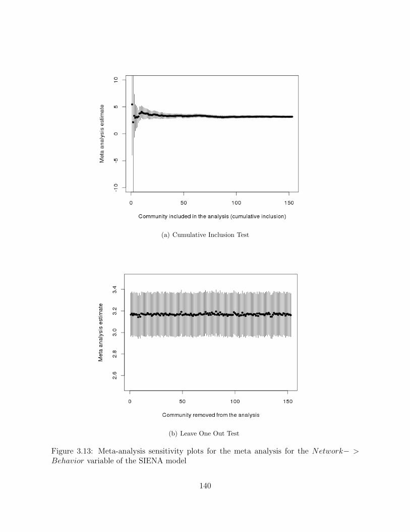
(a) Cumulative Inclusion Test

(b) Leave One Out Test

Figure 3.13: Meta-analysis sensitivity plots for the meta analysis for the Network− >Behavior variable of the SIENA model

140

Figure 3.14: Meta-analysis diagnostic plots for the Network− > Behavior variable of theSIENA model

141

Table 3.25: Results of the meta-analysis for each of the behavioral and network effectsincluded in the SIENA model

Time name coeff stderr pval I2 H2 τ2 Q-Test Q-Test N obsPart. (p-val)

[1;2

]−[3

;11] outdegree (density) -4.214 0.052 0.000 62.458 2.664 0.169 325.644 0.000 104

reciprocity 5.014 0.090 0.000 59.418 2.464 0.421 269.346 0.000 104transitive ties 2.539 0.045 0.000 56.025 2.274 0.113 263.453 0.000 104Behavior− > Network 0.011 0.069 0.875 34.931 1.537 0.134 164.549 0.000 104Network− > Behavior 3.347 0.107 0.000 0.000 1.000 0.000 43.340 1.000 104

[1;3

]−[4

;11]

outdegree (density) -4.393 0.043 0.000 59.972 2.498 0.167 448.472 0.000 150reciprocity 4.772 0.079 0.000 72.366 3.619 0.530 595.384 0.000 150transitive ties 2.377 0.035 0.000 52.279 2.095 0.095 351.168 0.000 150Behavior− > Network 0.056 0.051 0.269 26.986 1.370 0.084 213.184 0.000 150Network− > Behavior 3.156 0.094 0.000 0.000 1.000 0.000 58.394 1.000 150

[1;5

]−[6

;11] outdegree (density) -4.370 0.053 0.000 66.291 2.967 0.204 374.884 0.000 112

reciprocity 4.107 0.073 0.000 75.442 4.072 0.404 475.923 0.000 112transitive ties 1.939 0.036 0.000 47.098 1.890 0.070 230.529 0.000 112Behavior− > Network 0.037 0.054 0.498 29.333 1.415 0.077 167.707 0.000 112Network− > Behavior 2.857 0.232 0.000 27.452 1.378 2.014 121.619 0.231 112

[1;6

]−[7

;11] outdegree (density) -4.443 0.057 0.000 65.275 2.880 0.214 337.356 0.000 102

reciprocity 3.896 0.070 0.000 67.843 3.110 0.295 324.878 0.000 102transitive ties 1.723 0.042 0.000 53.516 2.151 0.096 228.744 0.000 102Behavior− > Network 0.069 0.054 0.199 26.291 1.357 0.065 144.909 0.003 102Network− > Behavior 3.112 0.130 0.000 0.000 1.000 0.000 24.392 1.000 102

[1;7

]−[8

;11] outdegree (density) -4.504 0.061 0.000 65.212 2.875 0.226 299.468 0.000 92

reciprocity 3.777 0.073 0.000 65.190 2.873 0.286 264.460 0.000 92transitive ties 1.495 0.042 0.000 48.672 1.948 0.079 186.580 0.000 92Behavior− > Network 0.054 0.060 0.374 26.053 1.352 0.061 147.948 0.000 92Network− > Behavior 3.173 0.129 0.000 0.000 1.000 0.000 16.742 1.000 92

[1;8

]−[9

;11] outdegree (density) -4.845 0.077 0.000 52.680 2.113 0.189 125.514 0.000 58

reciprocity 3.935 0.104 0.000 62.745 2.684 0.394 175.865 0.000 58transitive ties 1.275 0.053 0.000 35.695 1.555 0.055 90.531 0.003 58Behavior− > Network 0.204 0.089 0.026 32.069 1.472 0.110 94.797 0.001 58Network− > Behavior 3.191 0.134 0.000 0.000 1.000 0.000 5.989 1.000 58

[1;9

]−[1

0;11

]

outdegree (density) -5.118 0.133 0.000 62.162 2.643 0.339 103.864 0.000 30reciprocity 4.072 0.158 0.000 52.273 2.095 0.354 65.433 0.000 30transitive ties 1.082 0.084 0.000 51.543 2.064 0.096 64.265 0.000 30Behavior− > Network 0.138 0.093 0.148 0.001 1.000 0.000 29.795 0.424 30Network− > Behavior 2.664 0.183 0.000 0.000 1.000 0.000 2.410 1.000 30

[1;1

0]−

11

outdegree (density) -5.539 0.259 0.000 39.885 1.663 0.222 14.597 0.067 9reciprocity 4.071 0.329 0.000 31.055 1.450 0.241 13.649 0.091 9transitive ties 0.860 0.164 0.001 36.805 1.582 0.066 15.223 0.055 9Behavior− > Network 0.319 0.167 0.093 0.001 1.000 0.000 7.541 0.480 9Network− > Behavior 2.051 0.372 0.001 0.000 1.000 0.000 0.431 1.000 9

Note 1: variable Behavior− > Network is captured by the behaviorsimilarity SIENA effect;Note 2: variable Network− > Behavior is implemented through the behavioraveragesimiliratySIENA effect; Note 3: Meta analysis estimated through Maximum Likelihood assuming a randomeffects model with Knapp and Hartung standard error correction; Note 4: τ2 is the estimate of totalamount of heterogeneity, I2 is the % of total variability due to heterogeneity, H2 is totalvariability

samplingvariability .

142

Table 3.26: Results of the meta-analysis for each of the behavioral and network effectsincluded in the SIENA model

Time name coeff stderr pval I2 H2 τ2 Q-Test Q-Test N obsPart. (p-val)

[1;3

]−[4

;6]−

[7;1

1]

outdegree (density) -4.195 0.038 0.000 69.841 3.316 0.107 392.527 0.000 104reciprocity 4.029 0.059 0.000 82.368 5.672 0.290 708.874 0.000 104transitive ties 1.833 0.028 0.000 57.796 2.369 0.046 265.849 0.000 104Behavior− > Network 0.012 0.037 0.748 37.558 1.601 0.052 163.277 0.000 104Network− > Behavior 3.040 0.111 0.000 0.000 1.000 0.000 43.034 1.000 104

[1;4

]−[5

;8]−

[9;1

1]

outdegree (density) -4.320 0.051 0.000 71.312 3.486 0.129 272.047 0.000 73reciprocity 3.884 0.072 0.000 81.336 5.358 0.288 419.031 0.000 73transitive ties 1.677 0.039 0.000 64.556 2.821 0.067 211.380 0.000 73Behavior− > Network 0.067 0.042 0.113 25.463 1.342 0.031 97.622 0.024 73Network− > Behavior 3.009 0.133 0.000 0.000 1.000 0.000 25.781 1.000 73

Note 1: variable Behavior− > Network is captured by the behaviorsimilarity SIENA effect;Note 2: variable Network− > Behavior is implemented through the behavioraveragesimiliratySIENA effect; Note 3: Meta analysis estimated through Maximum Likelihood assuming a randomeffects model with Knapp and Hartung standard error correction; Note 4: τ2 is the estimate of totalamount of heterogeneity, I2 is the % of total variability due to heterogeneity, H2 is totalvariability

samplingvariability .

143

144

Chapter 4

The Impact of Likes on the Sales of

Movies in Video-on-Demand: a

Randomized Experiment

Abstract: We designed and implemented a randomized field experiment to determine the

role that likes play on the sales of movies in Video-on-Demand (VoD). We used the VoD

system of a large telecommunications provider during half a year in 2012. The VoD system

of this provider suggests movies to subscribers when they log in. Suggested movies are

displayed on the TV screen under several editorial menus. Under each menu movies are

shown from left to right in decreasing order of the number of likes received. During our

experiment, movies were primarily placed in their true slots and shown along with their

true number of likes. At random moments, some movies were swapped and thus displayed

out of order and with a fake number of likes. The movies that were swapped were selected

at random. We found that promoting a movie by one slot increased weekly sales by 4% on

average. We found that the amount of information publicly available about movies affected

this statistic. Better known movies were less sensitive to manipulations. We found that a

movie promoted (demoted) to a fake slot sold 15.9% less (27.7% more) than a true movie

placed at that slot, on average across all manipulations we introduced. We also found that

a movie promoted (demoted) to a fake slot received 33.1% fewer (30.1% more) likes than

145

a true movie at that slot. Therefore, manipulated movies tend to move back to their true

slot over time. Hence, we find that the self-fulfilling prophecies widely discussed in the

literature on the effect of ratings on sales are hard to sustain in a market in which goods

are costly and sufficiently well-known. During this adjustment process, providers are likely

to enjoy increased profits while subscribers might lose welfare. This process is likely to

converge quickly, which might lead the telecommunications provider to promote different

movies over time.

4.1 Introduction

Figure 4.1 shows that home video revenues have increased substantially since the 1970s

while theater revenues have remained constant over time. One can still argue that the

success of a movie dependents highly on box office sales because exhibition in theaters not

only allows for covering a significant part of the cost to produce a movie but also trig-

gers demand in subsequent channels. However, it is clear that digitization is changing the

structure of the industry. In particular, the share of Video-on-Demand (VoD) and Pay-

Per-View (PPV) in the electronic spending on movie rentals in the US increased roughly 4

times between 2000 and 2009. Brick and mortar’s share reduced roughly 50% during the

same period of time (Waterman, 2011).

VoD providers such as Amazon, Netflix or Hulu have catalogs with more than 100,000

titles (Rowinski, 2011), whereas traditional brick and mortar stores offer catalogs with no

more than 3,000 titles (Anderson, 2006). Economic theory predicts that product variety

increases consumer welfare (Hotelling, 1929; Dixit and Stiglitz, 1977; Salop, 1979). How-

ever, search costs also increase with the number of products that consumers need to scan.

146

Figure 4.1: Revenues of movie distributors in the US market as a percentage of GDP(excluding merchandising). Source: (Waterman, 2011)

Therefore, consumers may be unable to internalize the benefits of increased variety (Nelson,

1970; Sawhney and Eliashberg, 1996). In fact, a number of studies have reported a negative

relationship between product variety and sales. For example, (Iyengar and Lepper, 2000)

showed that increasing the variety of flavors of a specific jam product in a supermarket

reduced consumer willingness to buy. (Boatwright and Nunes, 2001) showed that reducing

the number of stock keeping units in a grocery store had a positive impact on sales. More

recently, (Kuksov and Villas-Boas, 2010) developed a theoretical model that shows that

excess variety increases consumer search costs and reduces total sales.

Product variety can increase consumer welfare if more efficient search mechanisms be-

come available. This is particularly true in the movie industry. Several surveys in the US

show that consumers welcome recommendations on which movies to watch (De Vriendt

et al., 2011), probably because movies are an example of an experience good (Nelson,

1970), (Eliashberg and Shugan, 1997): their quality can only be ascertain after consump-

147

tion. 45% of the people surveyed by Ovum in 9 countries around the world welcomed

suggestions from friends when searching for new movies to watch (Little, 2010). Tapping

into this opportunity, several companies are now implementing recommender systems to

provide suggestions to their clients. Again, Hulu, Netflix and Amazon are widely known

examples. These companies incorporate rating mechanisms in their recommender systems

whereby consumers are allowed to express whether they liked the content they purchased.

Determining the true impact of rating systems on sales is a challenging empirical ques-

tion. Observational studies are often subject to the reflection problem (Manski, 1993),

which hampers the identification of the impact of group behavior on individual decisions.

As such, many observational studies offer conflicting perspectives. For example, (Eliash-

berg and Shugan, 1997) concludes that ratings from movie critics are not good predictors

of sales, whereas (Reinstein and Snyder, 2005) concludes otherwise. Several authors used

experiments to try to obtain identification. For example, (Salganik et al., 2006) studied

the effect of popularity in a market of songs from obscure bands. (Tucker and Zhang, 2011)

studied the effect of popularity across wedding service vendors. These studies show that

popularity can be, to a certain extent, self-reinforcing. However, they do not explicitly

control for the quality of the experience obtained by consumers.

In this paper, we design a randomized experiment to determine the role that social

signals play on the sales of VoD products. We use the VoD system of a large telecom-

munications provider (at which subscribers need to pay to lease movies). Our experiment

148

run live for half a year during 2012. The popularity of a movie in the VoD system of

this provider is encoded by the order in which the movie is displayed on the TV screen,

hereinafter called the rank, which is a function of the number of likes issued by subscribers.

A movie with a higher number of likes is shown farther to the left on the TV screen. Dur-

ing our the experiment, movies were primarily placed in their true rank and shown along

with their true number of likes. At random moments, some movies were swapped and

thus displayed ”our of order” and with a fake number of likes. The movies swapped were

randomly selected. These random exogenous shocks allow for disentangling the perceived

quality from the true quality of a movie, thus allowing us to obtain unbiased estimates for

the effect of popularity on VoD sales.

We find that on average weekly sales increase by 4% when a movie is promoted one

rank. We also find that the weekly sales of a movie promoted (demoted) to a better (worse)

rank are 15.9% lower (27.7% higher) than those of a movie placed at that rank by the num-

ber of likes issued by subscribers, on average across all manipulations we introduced. We

show that this asymmetry is related to the amount of information publicly available about

the movies manipulated, as measured by number of IMDb votes. Better-known movies are

less sensitive to our manipulations. We also find that a movie promoted (demoted) to a

better (worse) rank receives 33.1% fewer (30.1% more) likes than a movie placed at that

rank by the number of likes issued by subscribers. Therefore, manipulated movies tend to

move back to their true rank over time. This means that self-fulfilling prophecies are hard

to sustain in a market in which goods are costly and sufficiently well known. Finally, we

149

provide evidence that during this process of adjustment, the provider may enjoy increased

profits while subscribers may lose welfare, as measured by the number of likes issued. This

process is likely to converge quickly, which might lead the provider to promote different

movies over time.

4.2 Related Literature

Most papers looking at the impact of quality signals in the movie industry are observational

and offer contradictory perspectives. (Litman, 1983) and (Wallace et al., 1993) analyzed

125 and 1687 movies, respectively, released in the US between 1972-78 and 1956-88, respec-

tively. Both report a positive correlation between box office sales and reviews by movie

critics. However, (Eliashberg and Shugan, 1997) found that ratings from movie critics

are not good predictors of sales during the opening week. They argue that despite being

correlated with cumulative movie sales, these ratings do not influence sales in a causal sense.

(Godes and Mayzlin, 2004) studied 44 TV shows released in the US between 1999 and

2000. They found that the dispersion in Word-of-Mouth (WoM) about these shows across

distinct groups in Usenet (a news aggregator) was positively correlated to their ratings.

However, they were unable to establish a link between WoM, measured by number of con-

versations about a show, and future rankings, which correlate to sales. (Liu, 2006) studied

data from message boards at Yahoo Movies! about 40 movies released between May and

September 2002 in the US. They found that the volume of WoM was positively correlated

150

with box office sales but they could not establish a statistically significant relationship

between the direction implied in the messages (positive/negative comments) and sales.

A number of previous studies fail to account for the potential correlation between un-

observed quality and ratings and therefore are unable to investigate the causal mechanisms

that might be at the root of the impact of reviews on sales. Other papers have attempted

to overcome this concern. For example, (Reinstein and Snyder, 2005) applied a difference

in difference model to a sample of more than 600 movies rated by two influential movie

critics to try to identify the marginal impact of reviews on sales. Using the fact that some

movie reviews were issued prior to the release of the movie while others were issued after

the opening week, they showed that ratings from movie critic were positively correlated

with sales and influenced box office sales during the opening week, which again contradicts

the findings in (Eliashberg and Shugan, 1997).

(Zhang and Dellarocas, 2006) developed a structural model to study the impact of

consumer and movie critic ratings on sales. They showed that good reviews drove movies

sales but that the volume and dispersion of the reviews did not. (Dellarocas et al., 2007)

developed a predictive model for movie sales that showed that the volume, valence and

dispersion of reviews were all positive and statistically significant predictors of box office

sales. Finally, (Duan et al., 2008) proposed a model with simultaneous equations to esti-

mate user movie ratings and movie box office sales simultaneously. They concluded that

WoM is a strong driver of box office sales, which contradicts the findings in (Zhang and

151

Dellarocas, 2006). Therefore, there is substantial conflict even across the studies that at-

tempt to control for unobserved quality.

A number of authors used experiments to better overcome the traditional hindrances

of observational studies. These studies analyze the impact of popularity on sales in the

context of other industries. In a seminal paper, (Salganik et al., 2006) created two virtual

markets for songs from unknown bands and recruited a group of subjects on a website for

teenager interests. Each subject was randomly assigned to one of these markets. Songs

were ordered randomly in one of the markets and ordered according to the number of

downloads in the other market. Subjects were asked to chose songs to listen, to rate them

and then to download them for free if they so wanted. Their study showed that the best

(worst) songs received more (less) downloads. The songs in between tended to receive ever

more (less) downloads when shown at a higher (lower) rank. In other words, popularity

was self-reinforcing for these songs.

In a follow-up study (Salganik and Watts, 2008) run a similar experiment using similar

songs and a similar pool of subjects. In a setup phase they ask participants to listen to the

songs and to rate them. Then they order songs according to these ratings so that better

songs would come last and thus seem worse. In this setting, they observed that over time

all songs (good or bad) tended to converge to their true download rank. Taken together,

these studies show that self-fulfilling prophecies in these markets are constrained by the

individuals’ private preferences.

152

A similar experiment was developed by (Tucker and Zhang, 2011). They used an online

hub for online wedding service vendors to explore the impact of popularity on the number

of clicks that each vendor obtained. They displayed vendors in three categories. In one cat-

egory vendors were sorted in decreasing order of the number of clicks received. In another

category vendors were sorted in increasing order of the number of clicks received. In both

cases, vendors were listed along with the number of clicks received. In the last category

vendors were sorted alphabetically and no information on clicks received was displayed.

They compared vendors across different categories, before and during their experiment, to

determine the impact of popularity, measured by the number of clicks received, on future

clicks. They conclude that popularity is self reinforcing and that vendors that operate in

narrower markets benefit the most from this dynamics.

Our paper is different from these studies in some important dimensions. First, the pa-

pers by (Salganik et al., 2006) and (Tucker and Zhang, 2011) measure impact of popularity

on sales. They do not measure the impact of user feedback –likes – on sales. One expects

likes to reflect better the subscribers’ taste and assessment of quality. This is especially

true for experience goods like music and movies, for which more downloads typically lead

to more popularity and vice-versa. In our setting, more likes may lead to more purchases.

However, the decision to provide likes in our case is tightly related to the quality of the

movies watched. In short, we believe that likes are a better and stronger measure of quality

than the popularity measures used in previous studies. In (Salganik et al., 2006) downloads

153

might proxy whether subjects like songs but in their settings they are only a noisy measure

of preferences across songs.

Another important difference in our setting is that the goods are not free. Subscribers,

in our setting, have to make explicit decisions that involve financial risks. The price to rent

movies in the VoD system of our Industrial Partner (IP varied between $1.30 and $5.20.

In (Salganik et al., 2006) and (Salganik and Watts, 2008) songs could be downloaded for

free. Subjects did not incur any financial risk in either listening or downloading a song.

(Tucker and Zhang, 2011) observe click through rates on websites but they know nothing

about actual purchase decisions. It is not clear how the results of these studies generalize

to goods that are not free. For example, in (Salganik and Watts, 2008) demoted songs

eventually recover to their true rank. However, this may be an artifact of the fact that

songs were provided for free. Since subjects could easily buy several songs, songs in lower

ranks may benefit more than demoted movies in our setting.

Another key distinction is that (Salganik et al., 2006) used mostly obscure songs. Thus,

downloads provided almost all the information about these songs to the subjects in the

study. In most real settings goods are not as unknown to consumers. Consumers can get

some information about the quality of products from many external sources. In such set-

tings, the informativeness of likes is unclear. We also note that in our setting subjects are

real customers of our IP. Our experiment was conducted live in the real field. While this im-

poses some challenges to carry it out, it also makes for a unique, general and robust setting.

154

Finally, our paper goes beyond estimating the effect of rank changes on sales. In par-

ticular, we are interested in estimating the social cost of changes in rank. Social cost in

our context is measured by the loss in sales, or by the loss in likes, when ranks are ma-

nipulated. For example, we seek to measure if a movie manipulated into a particular rank

sells as much as the correct movie at that rank. Most of the prior work has focused on

how rank changes affect sales but not on the social cost associated with these manipulations.

4.3 The Context of Our Experiment

4.3.1 The Company and its Dataset

Our experiment was performed using a real world VoD system from a major telecommu-

nications provider, hereinafter called Industrial Partner (IP). Our IP offers TV, Internet,

telephone and mobile phone service. IP is the market leader of Pay-TV services in the

country where it operates. It services approximately 1.5 million households, 69% of which

purchase triple play bundles that include TV, Internet and fixed telephony. According

to a market report published by Screen Digest, 65% of the households in this country

subscribed to Pay-TV services by the end of 2012. The same report shows that 46% of

households with Pay-TV obtained service over cable, 23% over IPTV and the remaining

28% over satellite. Our IP offers Pay-TV through both wired connections and satellite.

155

We had access to our IP’s VoD database between February 2009 and December 2012,

which includes information on all of its 3,408,995 subscribers, of which 1,479,895 are on

average active at any point in time. 623,516 of the active subscribers buy services that

include VoD. Overall, 681,036 subscribers watched VoD content at least once and 465,059

subscribers paid for VoD content at least once during this 41-month period. The remaining

subscribers with VoD capabilities never used the service. We also had access to all (paid

and free of charge) VoD transactions. During this period we observe 89,074,657 transac-

tions, of which 6,293,557 correspond to paid leases.

We have the anonymized identifier of the subscriber requesting each (and every) trans-

action as well as the anonymized identifier for the MAC address of the specific Set-Top

Box (STB) that did so. For each transaction we have a timestamp, the price and the

identifier of the movie leased. For each movie in our IP’s database we have title, director,

studio, play length, synopses, cast, genres, asset type (movie, music, documentary, etc).

We also have information on the daily layout of the TV screen that subscribers saw when

they logged into the VoD system between 11-2011 and 12-2012. This information includes

the tree of menus displayed as well as the order, hereinafter called rank, in which movies

were displayed under each menu on the screen from left to right. Menus are associated

with different editorial lines as described in the next section. Finally, we also have daily

information on all trailer views and on the number of likes issued to each (and every) movie.

156

4.3.2 VoD Service and Interface

Our IP provides service over wired and satellite infrastructure. However, satellite sub-

scribers cannot subscribe to VoD. Wired subscribers can obtain one of three types of

services: basic/legacy, standard or premium. All of them can watch TV and subscribe to

specific channels such as movies, sports, children’s and adults’ content, etc. As Figure 4.2

shows, only standard and premium subscribers can use VoD as well as some additional ser-

vices. For example, both of them can record content if their STB and network connection

so allow. Premium subscribers can also restart programs. They can also issue likes for

VoD movies and TV programs as well as connect their IP account to Facebook. They are

required to also subscribe Internet service. In this paper, we will focus only on standard

and premium subscribers. 84% of these subscribers were standard in January 2012. This

number reduced to 66% by the end of the year.

Figure 4.2: Summary of the main features available to subscribers of our IP.

The look and feel of the VoD screen for standard and premium subscribers is different

157

but the organization of content into menus is hierarchically similar. In fact, our IP does

not have the ability to suggest different movies to different subscribers, which has a major

impact on the way we designed our experiment, as described in the next section. Both

standard and premium subscribers can access the VoD system using a hot-key in their STB

remote control. When they press it, the entry screen of the VoD system is displayed. This

screen, called the Highlights Section, contains a set of menus filled with movies, chosen by

an editorial team, which are very easy to access. Movies are organized into menus such

as Promotions, Suggestions, Newest Releases, etc. Each menu has a header with a name

that clearly identifies the type of movies underneath it. Menus are horizontal lines on the

screen. Different menus are stacked vertically. Two menus fit on the screen at each time.

A cursor highlights a movie cover at a time. Users can scroll across menus. The natural

scrolling direction is down, though premium consumers can also scroll up.

Upon scrolling to a new menu, 8 movie covers are visible under that menu and the

cursor highlights the movie farthest to the left. Users can also scroll right and left at their

leisure within the same menu. Users can scroll right past the last movie cover on the screen

to unveil hidden movies under the same menu. There is no limit for the number of movies

under a menu though our IP displays no more than 15 movies per menu. The screen of a

standard subscriber is somewhat different. Menus show only 4 movies and only 11 other

movies can be accessed by scrolling right.

The title and number of likes of the movie highlighted by the cursor are shown on the

158

screen. Standard subscribers do not see the number of likes. Clicking on the cover of a

movie leads to a new screen with the year of release, play length, cast, synopsis and number

of likes (the latter only in the case of premium subscribers). A number of actions are then

available such as lease the movie, use a promotional coupon to lease the movie or watch

the movie trailer (if one is available). Premium subscribers can also signal whether they

like the movie.

Finally, subscribers can leave the Highlights Section of the VoD interface and search

for movies in the complete Catalog of titles. The catalog is hierarchically organized into

content categories such as movies, music, TV-shows, documentaries, etc. Within each of

these category screens are organized as described above with menus for genres. Alterna-

tively to browsing through the entire catalog, subscribers can use a keyword search to look

for the content of their interest. They can use words that identify titles, movie directors

and actors’ names.

We note that the likes feature, visible only for premium subscribers, replicates Face-

book’s well known like button1. The number of likes shown along with movie covers is

cumulative since the movie’s debut at our IP’s VoD. Subscribers do not know who liked a

particular movie nor who and how many people leased a particular movie.

1Premium subscribers can also notify IP that they dislike a movie but the number of dislikes is notshown.

159

4.4 Experimental Design

A new menu named ”The Most Popular During the Past Weeks” was introduced in the

highlights Section of IP’s VoD system on July 3rd 2012. This menu was available for both

standard and premium subscribers and included the 15 movies that obtained the highest

number of likes in the last few weeks. These movies were shown under this menu in de-

creasing order of this number of likes from left to right. The experiment run in 1-month

cycles for a period of 6 consecutive months. Each cycle was further split into mini-cycles

of 1 week each2. Weeks were named true or false. During a true week all movies under this

menu were shown in their true rank. The true number of likes they obtained in the recent

past was shown to premium consumers. During a false week a carefully devised random-

ization procedure was used to swap some movies under this menu to separate popularity

from unobserved perceived movie quality.

Formally, the experiment ran as follows. Let ti represent the time at which cycle i be-

gan, with i ∈ {1, 2, 3, 4, 5, 6}. Let x represent a week’s time. At time ti, we sorted all movies

in IP’s VoD system according to the number of likes they received between ti − 2x and ti.

From this list we erased all movies that IP decided to use in other menus under the high-

lights section3. We kept the 45 movies at the head of the resulting list, which we call list L.

2Each week started at a time of low VoD usage, namely Tuesdays at around 2pm.3IP decided to list some of these movies under other menus such as Promotions and Suggestions. Clean-

ing them from our list avoided displaying them under more than one menu in the highlights section, whichwould notoriously reduce their search cost. Furthermore, IP’s log system does not allow for identifying themenu under the highlights section from which a lease originates and thus this cleaning procedure allowsalso for ensuring that leases of movies under the new menu came only from the new menu.

160

After the setup phase described above, which took place at the beginning of each cycle,

a true week ensued to adjust the subscribers’ expectations to the true quality of the movies

show under the new menu. We determined the nature of each of the other 3 weeks within

every cycle using a coin toss4. This allowed us to prevent a static pattern of true/false

cycles that subscribers could perceive. Table 4.1 shows the order of true and false cycles

used in our experiment.

Table 4.1: Cycles and the nature of sub-cycles during our experimentCycle 1 t1: True t1 + x: True t1 + 2x: False t1 + 3x: FalseCycle 2 t2: True t2 + x: False t2 + 2x: True t2 + 3x: FalseCycle 3 t3: True t3 + x: False t3 + 2x: False t3 + 3x: TrueCycle 4 t4: True t4 + x: False t4 + 2x: False t4 + 3x: FalseCycle 5 t5: True t5 + x: False t5 + 2x: False t5 + 3x: FalseCycle 6 t6: True t6 + x: False t6 + 2x: True t6 + 3x: False

At the beginning of each true week we sorted all movies in L according to the number

of likes that they obtain between ti − 2x and ti + nx with n ∈ {1, 2, 3} indicating how

many weeks elapsed since the start of the current cycle. We displayed under the new menu

the first 15 movies in L from left to right on the TV screen. At the beginning of each

false week we partitioned L into 3 sub-lists. List L1 comprised the 15 movies at the head

of list L. List L2 included the movies between ranks 16 and 30 in list L. Finally, list L3

contained the movies positioned between ranks 31 and 45 in list L. Then, we performed

the following swaps:

• Within Swap: we selected yi and yj randomly from {1, ..., 15} such that yi 6= yj and

we swapped the number of likes associated with the ythi and ythj movies in list L1;

4The coin used was biased to try to ensure a balance between true and false across the whole experience.

161

• Between Swap: we selected zi randomly from {1, ..., 15} such that zi 6= yi and zi 6= yj

and we selected zj randomly from {1, ..., 15}. Then, we swapped the number of likes

of the zthi movie in list L1 with the number of likes of the zthj movie in either list L2

or list L3, as determined below.

The movies in list L1 were then displayed under the new menu from left to right on the

TV screen. The two types of random swaps introduced with this experiment were aimed at

capturing the particular characteristics of the look and feel of IP’s VoD interface. Within

Swaps allow for determining whether changes in ranks across the movies displayed under

the new menu have an impact of sales. Between Swaps allow for determining the impact

of bringing movies from the catalog into the new menu and of removing movies from the

new menu into the catalog. A Within swap changes the search cost of the swapped movies

only slightly but a Between Swap reduces substantially the search costs for a movie that

is promoted from the catalog to the new menu and increases substantially the search costs

for a movie that is demoted from the new menu into the catalog.

We performed two Within Swaps and one Between Swap at each false week during the

first three cycles of our experiment. The latter alternated between lists L2 and L3. We

performed three Within Swaps and two Between Swaps at each false week, one involving

L2 and one involving L3, during the last three cycles of our experiment. We increased the

frequency of swaps in the final three cycles of the experiment to increase the number of

treated observations5.

5Whether a week is true or false is still randomly determined and therefore unrelated to sales duringour experiment (results are available upon request).

162

4.5 Empirical Model

4.5.1 Movie Level Specification

The demand for a movie is given by:

yit = α + xitβ + witγ + ziδ +mi + uit, t = 1, . . . T (4.1)

yit represents the sales of movie i during week t, xit includes time varying observed movie

characteristics such as age, rank and the number of distinct menus where the movies shows

up, wit is the vector of our exogenous random treatments, zi includes time invariant ob-

served movie characteristics such as genre, cast and price, mi are time constant unobserved

movie fixed effects, such as the quality of the movie’s story line, and uit is the idiosyncratic

error term. This equation is the classical fixed effects specification, which we can estimate

if we eliminate mi. We use first differences with robust standard errors to do so given

the potential for serial correlation in uit (Wooldridge, 2010). Therefore, we estimate the

following model:

∆yit = ε+ ∆xitβ + ∆witγ + ∆uit, t = 2, . . . T (4.2)

Note that the time constant movie fixed effects in zi drop despite being observed. In

particular, the retail price drops from our regression. Price includes a fixed margin on the

top of the royalty fee and the latter did not change during our experiment. Furthermore,

prices do not respond to changes in demand in our setting. IP does not engage in dynamic

163

pricing and the network costs to stream VoD content are essentially negligible.

4.5.2 The Magnitude of Treatment

Consider movies A and B under the new menu in ranks a and b, respectively, at time

ti + nx, with n < 3. When these movies are swapped their new ranks in list L are, mo-

mentarily, b and a, respectively. At time ti + (n + 1)x, movies in this list are reordered

according to number of likes as described in section 4.4. As a result, assume that the movie

at rank a shifts to rank a′ and the movie at rank b shifts to rank b′. Subscribers see only

the cumulative effect of swaps and sorting. Thus, from their perspective, movie A moved

from rank a to rank b′ (a change of b′ − a ranks) and movie B moved from rank b to rank

a′ (a change of a′ − b ranks).

If the swap did not occur then subscribers would have seen that movie A moved from

rank a to rank a′ and movie B moved from rank b to rank b′. Therefore, the effect of

the random exogenous swap is given by (b′ − a) − (a′ − a) = b′ − a′ for movie A and by

(a′−b)−(b′−b) = a′−b′ for movie B. Note that this difference is zero for control movies. We

introduce this difference, which hereinafter we call rank manipulation, into ∆wit in equa-

tion 4.2. We code it so that it is positive when a movie is promoted and negative when a

movie is demoted. Also, a′ and b′ are the true ranks for movie A and B, respectively, which

hereinafter we call rank true. Therefore, we have rank = rank true−rank manipulation.

164

4.5.3 Identification and Exogeneity

Identification is obtained by design in our setting. In equation 4.2, ∆wit is not correlated

to ∆uit because movie swaps are randomly and exogenously determined. The two movies

involved in a swap are randomly selected. Therefore, not only movies are treated at random

but also the magnitude of treatment is random. In addition, the moments at which movies

are swapped are also randomly selected. Random assignment of treatment also ensures

that ∆wit is uncorrelated to ∆xit. In fact, Table 4.2 shows that the descriptive statistics

for the covariates in xit are similar for control and treated movies. Therefore, our estimates

for γ in Equation 4.2 are unbias

4.5.4 Rank Level Specification

Movies are reordered according to the number of likes at the beginning of each week. This

establishes a truthful relationship between rank and perceived quality for control movies

at the eyes of IP subscribers. Therefore, we can compare the sales obtained by control

and treated movies at each rank and determine whether promoted and demoted movies

sell differently than true movies placed at that rank. A true movie at a rank is a movie

that was placed at this rank as a result of the number of likes obtained from subscribers

and not as a result of one of our manipulations. If they do not then rank alone determines

movie sales. To test this hypothesis we use the following model:

yrt = α + xrtβ + wrtγ +mr + urt, t = 1, . . . T (4.3)

165

yrt represents the sales of the movie at rank r during week t, xrt includes observed

characteristics of the movie at rank r in week t such as age, price, IMDb rating and the

number of distinct menus where the movie shows up, mr is the intrinsic perceived quality

of rank r and urt is the idiosyncratic error term. wrt is a vector of exogenous random

treatments indicating whether the movie at rank r in week t was promoted, demoted

or neither. A promoted movie should have, on average, lower quality than the movie it

displaces and possibly sell less. Conversely, a demoted movie should have, on average,

higher quality than the movie it displaces and possible sell more. We estimate Equation

4.3 using a dummy variable for each rank.

4.6 Results and Discussion

4.6.1 Descriptive Statistics

The stock of VoD enabled subscribers at IP grew from 607 thousand in January 2012 to

633 thousand in December 2012. The share of VoD-enabled premium subscribers increased

from 16% to 34% during the same period. In the first half of 2012 premium users leased an

average of 1.1 thousand movies per day. This increased to 1.2 thousand during the second

half of the year. These statistics were 2.3 thousand and 1.7 thousand, respectively, for

standard users. Yet, the average number of leases per subscriber decreased from 3.2 to 1.1

from the first to the second half of the year for premium subscribers. These statistics were

1.8 and 1.5 for standard subscribers, respectively. During the first half of 2012, 75% of the

leases from premium users originated in the highlights section. This statistic increased to

166

79% in the second half of the year. These statistics were 64% and 68% for standard users,

respectively.

Figure 4.3 shows the 30-day moving average of daily sales in the highlights section

and in the catalog for premium and standard subscribers. Most sales came from standard

subscribers though this gap reduces significantly in the highlights section towards the end

of the year. Sales increased both in the highlights section and in the catalog around the

time the experiment started. The latter, however, declined significantly a few weeks into

the experiment. Panel (a) of Figure 4.4 shows the 30-day moving average of daily sales

for menus under the highlights section. This figure shows that the new menu was well

received by consumers and started selling well though not as much as the menus ”The

Most Seen” and ”New”. Sales in the new menu increased significantly during the first

10 weeks of the experiment as consumers became aware of it. Panel (b) provides more

details. After week 10 sales decreased in most menus. At week 10 IP introduced two new

menus into the highlights section, called ”The Most Seen of All Time” and ”IMDb’s Most

Popular”. These menus competed with the menu used for the experiment both in terms of

consumer attention and movies. In fact, when a movie under ”The most popular during the

past weeks” was also among ”The most seen of all times” or ”The most voted on IMDb” it

would be pulled into the latter two menus and deleted from the former to avoid duplication.

Figure 4.5 shows the weekly sales in the new menu over time. Unlike overall VoD con-

sumption, the majority of sales under this menu came from premium subscribers. Recall

167

(a) Leases from Standard Subscribers (b) Leases from Premium Subscribers

Figure 4.3: 30-Day Moving Average of Daily Leases in Highlights and Catalog in IP’s VoD.

(a) All Lines in Highlights (b) Zoom In the Experimental Line

Figure 4.4: 30-Day Moving Average of Daily Leases in Highlights per Menu in IP’s VoD.

that this menu was visible in the entry screen of the VoD system for premium subscribers

and reachable with 1 click up, whereas standard subscribers did not see this menu right

when they entered the highlights section and needed to click 10 times down to reach it. In

addition, standard subscribers do not see the number of likes, which might have rendered

this menu less meaningful to them.

Figure 4.6 shows the number of likes per rank in the beginning of each week. This

168

Figure 4.5: Sales in the New Menu During Our Experiment.

is a decreasing function by design. Yet, we observe a clear exponential decay. The most

liked movies seem to open a gap relative to the other ones. Figure 4.7 shows the number

of leases during the week per rank. This function, however, is far from monotone, which

might suggest that subscribers use more information besides rank and number of likes

to decide which movies to watch. Figure 4.8 shows the number of likes obtained during

the week as a function of rank. Panel (a) shows that the movies in the visible part of

the new menu tend to receive more likes than the movies in the hidden part of the menu.

Panel (b) shows that, on average, promoted (demoted) movies tend to receive fewer (more)

169

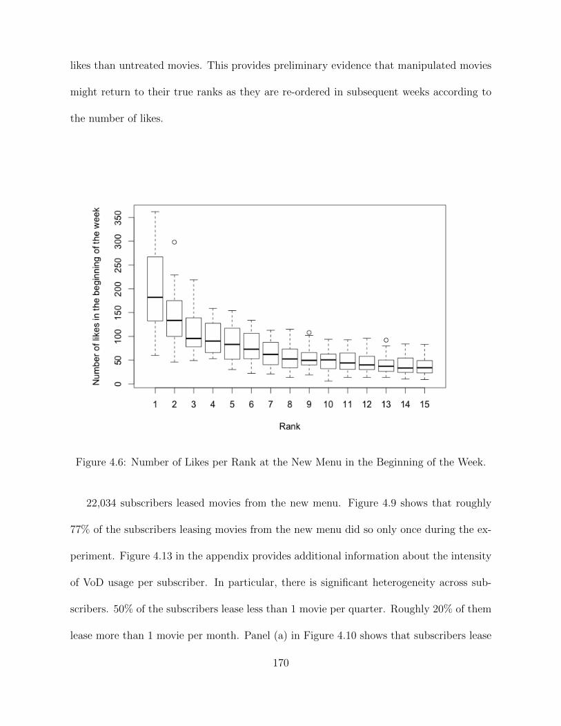
likes than untreated movies. This provides preliminary evidence that manipulated movies

might return to their true ranks as they are re-ordered in subsequent weeks according to

the number of likes.

Figure 4.6: Number of Likes per Rank at the New Menu in the Beginning of the Week.

22,034 subscribers leased movies from the new menu. Figure 4.9 shows that roughly

77% of the subscribers leasing movies from the new menu did so only once during the ex-

periment. Figure 4.13 in the appendix provides additional information about the intensity

of VoD usage per subscriber. In particular, there is significant heterogeneity across sub-

scribers. 50% of the subscribers lease less than 1 movie per quarter. Roughly 20% of them

lease more than 1 movie per month. Panel (a) in Figure 4.10 shows that subscribers lease

170

Figure 4.7: Leases per Week as Function of Rank at the New Menu.

(a) Likes per Week as a Function of Rank (b) Breakdown for Control vs. Treated Movies

Figure 4.8: Likes per Week as a Function of Rank for All, Control and Treated Movies atthe New Menu.

more movies after lunch and after dinner. Panel (b) in this Figure shows that subscribers

essentially lease movies during the weekend.

171

Figure 4.9: Statistics on VoD Consumption per Subscriber.

(a) Sales during the day (b) Sales over the week

Figure 4.10: VoD usage habits

172

Finally, Table 4.2 shows descriptive statistics for the covariates used in this paper

separately for all movies and for control and treated movies in the catalog and in the

highlights section. Essentially, control and treated movies are similar, as expected given

our random treatment assignment. T-tests to compare means between control and treated

movies show they are similar in all the covariates.

Table 4.2: Descriptive Statistics for Covariates used in this Paper.Catalog Highlights

Vars Stats All Control Treated Control Treatedn lease

mean 36.341 12.85 19.05 80.461 82.29sd 45.788 18.201 18.735 50.758 45.904

n lease premiummean 19.648 4.174 6.9 48.23 51.527sd 29.136 6.124 7.247 33.785 30.23

n lease standardmean 16.693 8.676 12.15 32.23 30.763sd 19.262 12.644 12.123 20.839 20.25

rankmean 13.311 16 16 8.531 7.151sd 4.487 0 0 4.197 4.369

rank truemean 13.348 16 8 8.531 9.28sd 4.438 0 4.472 4.197 5.247

rank manipulationmean 0.037 0 -8 0 2.129sd 2.5 0 4.472 0 6.811

n menusmean 1.984 1.708 1.65 2.609 2.258sd 1.058 0.932 0.813 1.193 0.674

pricemean 287.741 260.883 324 331.617 346.312sd 92.662 84.763 96.655 90.21 74.951

imdbratingmean 6.328 6.31 5.98 6.427 6.253sd 1.242 1.215 1.485 1.261 1.304

imdbvotesmean 82434.666 87387.516 73270.75 80008.728 58978.022sd 114271.836 117701.293 168947.22 111504.825 76944.554

movie agemean 250.257 291.779 266.294 166.844 187.112sd 380.553 415.368 429.838 277.441 314.458

Observations 1017 648 20 256 93

173

4.6.2 The Effect of Swaps and the Role of Rank

We estimate equation 4.4, which resembles equation 4.1, to learn the effect of rank on

leases. In this regression, treated within ∗ rank manipulation denotes the size of a rank

manipulation within the top 15 ranks. promoted to line and demoted from line denote

the size of rank manipulations that lead a movie to go from the catalog into the new menu or

to move from the new menu into the catalog, respectively. These 3 types of manipulations

constitute a partition of the space of possible manipulations and therefore their coefficients

must be interpreted relative to our control movies. treated indicates whether a movie has

been treated.

leasesit = λ+ β1log(movie ageit) + β2n menusit + β3treatedit +

β4rank trueit + β5treated within ∗ rank manipulationit +

β6promoted to lineit + β7demoted from lineit +

+week dummies+mi + εit (4.4)

Table 4.3 shows the results obtained with first-differences for all subscribers and sepa-

rately for standard and premium subscribers. The coefficient on treated within∗rank manipulation

shows that a promoted (demoted) movie receives more (fewer) leases. This result is statis-

tically significant for both standard and premium subscribers, although less for the former.

On average, a manipulation that increases rank by 1 leads to 2.313 (0.509) more leases

from premium (standard) subscribers. This corresponds to a 4.7% (1.6%) increase in the

174

number of leases. Promoting a movie to the new menu increases 7.2 (2.1) times the num-

ber of leases from premium (standard) subscribers, on average. This significant jump is

associated to the difference in search costs between the catalog and the highlights section.

Demoting movies from the new menu yields the opposite effect for premium subscribers.

The number of leases reduces by 37%. The effect of demotions from the new menu is not

statistically significant for standard subscribers. The new menu was much harder to reach

for standard subscribers and thus standard subscribers that use this menu might already

be more willing to search for good movies. Finally, the coefficient on treated is not statisti-

cally significant as expected given the random assignment of treatments in our experiment.

During our experiment, movies were primarily shown in their true rank. However,

sometimes, they were also exogenously and randomly swapped and thus shown in a fake

rank. This variability allows us to study whether a movie placed in a fake rank sells

differently from a true movie placed at that rank. To do so, we estimate equation 4.5,

which resembles closely equation 4.3:

leasesrt = λ+ β1log(movie agert) + β2n menusrt + β3pricert + β4imdbratingrt +

β5promoted ∗ treated withinrt + β6demoted ∗ treated withinrt +

β7promoted ∗ treated betweenrt + β7demoted ∗ treated betweenrt +

+week dummies+ rank dummies+ genre dummies+ year release dummies+ εrt(4.5)

175

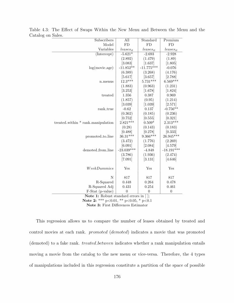
Table 4.3: The Effect of Swaps Within the New Menu and Between the Menu and theCatalog on Sales.

Subscribers All Standard PremiumModel FD FD FD

Variables leasesit leasesit leasesit(Intercept) -5.621* -2.693 -2.928

(2.892) (1.479) (1.89)[3.083] [1.637] [1.805]

log(movie age) -11.852** -11.775*** -0.076(6.389) (3.268) (4.176)[5.617] [3.657] [2.788]

n menus 12.3*** 5.731*** 6.569***(1.883) (0.963) (1.231)[3.253] [1.678] [1.824]

treated 1.356 0.387 0.969(1.857) (0.95) (1.214)[3.039] [1.039] [2.571]

rank true -0.62 0.137 -0.756**(0.362) (0.185) (0.236)[0.752] [0.555] [0.321]

treated within * rank manipulation 2.821*** 0.509* 2.313***(0.28) (0.143) (0.183)[0.488] [0.278] [0.333]

promoted to line 36.31*** 9.366*** 26.945***(3.472) (1.776) (2.269)[6.091] [2.084] [4.579]

demoted from line -23.039*** -4.848 -18.191***(3.786) (1.936) (2.474)[7.091] [3.131] [4.646]

WeekDummies Yes Yes Yes

N 817 817 817R-Squared 0.448 0.264 0.478

R-Squared Adj 0.431 0.254 0.461F-Stat (p-value) 0 0 0Note 1: Robust standard errors in [ ];

Note 2: *** p<0.01, ** p<0.05, * p<0.1Note 3: First Differences Estimator

This regression allows us to compare the number of leases obtained by treated and

control movies at each rank. promoted (demoted) indicates a movie that was promoted

(demoted) to a fake rank. treated between indicates whether a rank manipulation entails

moving a movie from the catalog to the new menu or vice-versa. Therefore, the 4 types

of manipulations included in this regression constitute a partition of the space of possible

176

manipulations and thus their coefficients must be interpreted relative to our control movies.

Table 4.4 shows the results obtained. The first three columns in this table show the

effect of rank manipulations on the number of leases whereas the last column shows the

effect of rank manipulations on the number of likes. A movie that is demoted to a fake

rank within the new menu sells 27.7% more than a true movie at that rank. Consumers

are still able to spot high quality movies even if they have been shifted to the right on the

TV screen under the new menu. This is true for both standard and premium subscribers

though less statistically significant for the former. These results suggest that subscribers

use more information besides rank to decide which movies to watch. We will provide more

details on this hypothesis later in this paper. Conversely, a movie that is promoted to a

fake rank within the new menu sells 15.9% less than a true movie at that rank. However,

this result is weaker than the effect of demotions within the new menu. Both its magnitude

and its statistical significance are lower. In fact, this effect is only statistically significant

for premium subscribers.

The last column in Table 4.4 shows the effect of promotions and demotions on the

number of likes obtained. A movie promoted (demoted) to a fake rank receives 33.1%

fewer (30.1% more) likes than a true movie at that rank. This result entails that over

time, manipulated movies are likely to come back to their true ranks. We will explore

this hypothesis in more detail later in this paper. In addition, note that the coefficients

for the effects of manipulations interacted with treated between are essentially statistically

177

Table 4.4: The Effect of Promotions and Demotions on Sales Relative to Movies at TrueRanks.

Leases LikesSubscribers All Standard Premium Premium

Variables leasesrt leasesrt leasesrt likesrt(Intercept) 63.134*** 0.986 62.148*** 45.615***

(21.573) (11.187) (13.157) (6.587)[18.904] [10.935] [10.906] [5.808]

promoted * treated within -12.184* -2.789 -9.396* -7.614***(4.773) (2.475) (2.911) (1.458)[7.308] [3.221] [5.108] [2.584]

demoted * treated within 22.348*** 7.756* 14.592*** 6.955***(4.749) (2.463) (2.896) (1.45)[7.034] [4.501] [4.21] [2.511]

promoted * treated between -4.331 1.09 -5.421 -7.853**(5.67) (2.94) (3.458) (1.731)[8.566] [3.391] [5.832] [3.156]

demoted * treated between 5.686 4.35* 1.336 1.241(5.718) (2.965) (3.487) (1.746)[4.448] [2.451] [2.524] [1.051]

log(movie age) -3.103*** -1.814*** -1.289** -0.305(0.727) (0.377) (0.443) (0.222)[1.178] [0.689] [0.633] [0.275]

n menus 4.000* 3.891*** 0.109 1.276**(1.115) (0.578) (0.68) (0.34)[2.106] [1.207] [1.063] [0.531]

price -0.005 -0.006 0.002 0.01*(0.016) (0.008) (0.01) (0.005)[0.026] [0.016] [0.013] [0.006]

imdbrating 3.541** 1.005 2.536** 1.112*(0.759) (0.394) (0.463) (0.232)[1.429] [0.717] [1.096] [0.576]

Week Dummies Yes Yes Yes YesRank Dummies Yes Yes Yes Yes

Genre Dummies Yes Yes Yes YesYear Release Dummies Yes Yes Yes Yes

N 1001 1001 1001 1001R-Squared 0.759 0.631 0.775 0.777

R-Squared Adj 0.697 0.58 0.713 0.714F-Stat (p-value) 0 0 0 0

Note 1: Robust standard errors in [ ]; Note 2: *** p<0.01, ** p<0.05, * p<0.1

insignificant, which means that search costs dominate the effect of manipulations. If any-

thing, standard subscribers lease demoted movies more than true movies, which provides

suggests that standard subscribers are more willing to search for movies to watch.

178

4.6.3 The Role of Outside Information

We test whether outside information about the movies shown at IP’s VoD system medi-

ates the effect of promoting and demoting movies. We use the number of IMDb votes as a

proxy for how well movies are known to consumers in general. The number of IMDb votes

indicates how may people evaluated a movie irrespective of the rating provided. Figure

4.11 shows that there is significant variation in the number of IMDb votes across movies in

our sample. This is not surprising given the well established super star effect in the movie

industry whereby popular movies concentrate a disproportionate amount of attention and

therefore are more widely known (Elberse and Oberholzer-Gee, 2006). In addition, both

IMDb votes and IMDb ratings are similar between control and treated movies. We hy-

pothesize that the movies in IP’s VoD system that have more outside information are less

sensitive to our exogenous random manipulations. This would be consistent in spirit with

the findings in (Tucker and Zhang, 2011) that show that products with broader appeal are

less likely to benefit from the popularity they obtain at the specific platforms where they

are sold6.

We classify each movie in our sample according to the number of IMDb votes received

until December of 2012. We define a dummy variable called top25 imdbvotes to indicate

whether a movie is in the top quartile of the distribution of IMDb votes in our sample.

6(Salganik and Watts, 2008) report a similar result but their measure of appeal is endogenous to thepopulation of subjects used in their experiment.

179

Figure 4.11: IMDb votes and ratings across movies in our sample.

We estimate equation 4.1 adding an interaction term between rank manipulation and

this dummy variable. In this regression, this interaction term captures the difference in

the effect of our rank manipulations for movies in the top quartile of the distribution

of IMDb votes relative to the effect on all the other movies in our sample that were

also manipulated. Table 4.5 presents the results obtained. The effect of the interaction

between rank manipulation and top25 imbdvotes is negative and statistically significant,

which confirms our hypothesis.

4.6.4 Converge to True Ranks

Figure 4.12 illustrates how manipulated movies converge to their true ranks over time.

The horizontal axes represent time relative to the moment of treatment. The vertical axes

180

Table 4.5: The role of IMDb Votes on the Effect of Rank manipulations on Leases.Subscribers All Standard Premium

Model FD FD FDVariables leasesit leasesit leasesit

(Intercept) -5.698* -2.723* -2.975*(2.883) (1.477) (1.885)[3.092] [1.647] [1.802]

log(movie age) -11.932** -11.807*** -0.125(6.369) (3.263) (4.165)[5.624] [3.665] [2.78]

n menus 12.346*** 5.749*** 6.597***(1.877) (0.962) (1.228)[3.268] [1.682] [1.833]

treated 1.193 0.323 0.87(1.852) (0.949) (1.211)[2.901] [1.037] [2.479]

rank true -0.674 0.115 -0.789**(0.361) (0.185) (0.236)[0.756] [0.559] [0.322]

treated within * rank manipulation 3.031*** 0.591* 2.44***(0.292) (0.149) (0.191)[0.51] [0.304] [0.345]

treated within * rank manipulation * top25imdbvotes -2.547** -1.001* -1.546**(1.037) (0.531) (0.678)[1.133] [0.552] [0.678]

promoted to line 36.439*** 9.416*** 27.023***(3.462) (1.773) (2.264)[6.031] [2.087] [4.532]

demoted from line -23.461*** -5.014* -18.447***(3.778) (1.935) (2.47)[6.736] [3.025] [4.439]

WeekDummies Yes Yes Yes

N 817 817 817R-Squared 0.452 0.267 0.482

R-Squared Adj 0.435 0.257 0.463F-Stat (p-value) 0 0 0

Note 1: Robust standard errors in [ ];Note 2: *** p<0.01, ** p<0.05, * p<0.1;

Note 3: First Differences Estimator

represent, for a particular time t in the horizontal axis, the average number of weekly leases

across all movies in our sample that were t weeks away from their treatment date. On the

top of each panel we indicate over how many movies each average is computed. Movies

tend to sell less over time before treatment mostly due to aging. Promoted (demoted)

181

movies sell significantly more (less) right after treatment. Within slightly more than 3

weeks promoted movies sell as much as they used to sell before treatment. For Demoted

movies the same is true, they need slightly more than 3 weeks to sell as much as they used

to sell before treatment.

Figure 4.12: Sales per Week for Promoted and Demoted Movies Before and After Treat-ment.

Manipulated movies may introduce changes in welfare, both for the profits of IP as well

as for consumers, though they converge relatively quickly to their true ranks. We compare

outcomes in false and true weeks to understand these changes.

Table 4.4 shows that sales during the week after a swap within the new menu increased

by 10.2. The average price of the movies in this menu during our experiment was $3.54 and

the average profit margin was 27% per movie. Therefore, IP enjoyed an additional profit

182

of $9.7 per within swap during the week after the swap. The additional profit associated

with premium subscribers is $4.99. Additionally, after a within swap premium subscribers

issued fewer 0.66 likes per week than before the swap. This is evidence that there are

changes in consumer surplus as a consequence of movie manipulations although we cannot

establish a monetary value for them with the data that we have available. Still our results

raise concerns about the effectiveness of recommender systems. While at the outset these

systems might be put in place to help consumers navigate large catalogs of options, in the

end the way firms manipulate them might be prejudicial for consumers. A recommender

system that uses likes from consumer to order the way alternatives are provided to them

seems to adjust quickly to extraneous disturbances and thus might help mitigate strategic

behavior.

4.7 Conclusions

In this paper, we design and implement a randomized experiment to determine the role

that likes play on the sales of movies over VoD. We use the VoD system of a large telecom-

munications provider during half a year in 2012. A new menu in the Highlights Section

of this VoD system was introduced showing the most liked movies in the past few weeks.

Movies with more likes were shown farthest to the left on the TV screen. During our the

experiment, movies were primarily placed in their true rank and shown along with their

true number of likes. At random moments, some movies were swapped and thus displayed

our of order and with a fake number of likes. The movies that were swapped were selected

183

at random. Randomization allows us to disentangle likes from unobserved perceived qual-

ity and thus estimate the effect of the former on sales.

We found that search costs play a major role on sales. A movie brought from the catalog

into the new menu sells about 7 times more, on average. We found that promoting a movie

by one rank increases weekly sales by 4% on average. We found that a movie promoted

(demoted) to a fake slot sells 15.9% less (27.7% more) than a true movie placed at that

slot, on average across all manipulations we introduced. We showed that this asymmetry

is related to the amount of information publicly available about the movies manipulated.

Better-known movies are less sensitive to manipulations.

We also found that a movie promoted (demoted) to a fake slot receives 33.1% fewer

(30.1% more) likes than a true movie at that slot. Therefore, manipulated movies tend

to move back to their true slot over time. During this adjustment process, the provider

enjoys increased profits while subscribers may lose welfare. This process is likely to con-

verge quickly, in a matter of 2 to 3 weeks time, which might lead the provider to promote

different movies over time to sustain its profit margin. However, it is not clear whether in

the long run subscribers will believe in the number of likes exhibited at this VoD system

if movies are manipulated often. Another way for the provider to attract attention to,

and possibly increase the sales of, specific movies without manipulating their rank is to

strategically show and hide movies between the Highlights Section and the catalog.

184

We have measured the impact of likes in a real VoD system of a large telecommunica-

tions provider. We believe that number of likes is a more truthful measure of the quality

experienced by subscribers than several popularity measures previously used in the liter-

ature. This is specially true in our setting, in which subscribers need to explicitly make

decisions that entail financial risks because movies are not free. Because movies are not

free in this setting, demoted movies could be unable to climb back to their true rank. We

showed they do at a slower pace than promoted movies fall back to their true rank. The

fact that movies are well known in our setting reduces the risk associated with choosing a

good but demoted movie. Certainly, trailers also allow subscribers to better perceive the

quality of a movie before they pay to watch it, which could benefit demoted movies as long

as subscribers are willing to search beyond the first ranked movies.

185

186

References

Chris Anderson. The Long Tail: Why the Future of Business is Selling Less of More.Hyperion, July 2006. ISBN 1401302378. 4.1

S. Berry, J. Levinsohn, and A. Pakes. Automobile prices in market equilibrium. Econo-metrica: Journal of the Econometric Society, page 841–890, 1995. 4.D

Steven T Berry. Estimating discrete-choice models of product differentiation. The RANDJournal of Economics, pages 242–262, 1994. 4.D

Peter Boatwright and Joseph C. Nunes. Reducing assortment: An attribute-basedapproach. Journal of Marketing, 65(3):50–63, July 2001. ISSN 0022-2429. URLhttp://www.jstor.org/stable/3203466. ArticleType: research-article / Full publi-cation date: Jul., 2001 / Copyright c© 2001 American Marketing Association. 4.1

Johan De Vriendt, Natalie Degrande, and Marc Verhoeyen. Video content recommendation:An overview and discussion on technologies and business models. Bell Labs TechnicalJournal, 16(2):235–250, September 2011. ISSN 1538-7305. doi: 10.1002/bltj.20513. URLhttp://onlinelibrary.wiley.com/doi/10.1002/bltj.20513/abstract. 4.1

Chrysanthos Dellarocas, Xiaoquan (Michael) Zhang, and Neveen F. Awad. Exploring thevalue of online product reviews in forecasting sales: The case of motion pictures. Journalof Interactive Marketing, 21(4):23–45, January 2007. ISSN 10949968. doi: 10.1002/dir.20087. URL http://linkinghub.elsevier.com/retrieve/pii/S1094996807700361.4.2

Dixit and Stiglitz. Monopolistic competition and optimum product diversity. The AmericanEconomic Review, Vol. 67(No. 3):297–308, 1977. 4.1

Wenjing Duan, Bin Gu, and Andrew B. Whinston. Do online reviews matter? —an empirical investigation of panel data. Decision Support Systems, 45(4):1007–1016,November 2008. ISSN 0167-9236. doi: 10.1016/j.dss.2008.04.001. URL http://www.

sciencedirect.com/science/article/pii/S0167923608000754. 4.2

Anita Elberse and Felix Oberholzer-Gee. Superstars and underdogs: An examination ofthe long tail phenomenon in video sales. Harvard Business School Working Paper Series,September 2006. 4.6.3

Jehoshua Eliashberg and Steven M. Shugan. Film critics: Influencers or predic-tors? Journal of Marketing, 61(2):68, April 1997. ISSN 00222429. doi:10.2307/1251831. URL http://www.jstor.org/discover/10.2307/1251831?uid=

3738880&uid=2129&uid=2&uid=70&uid=4&sid=21101210305387. 4.1, 4.2

David Godes and Dina Mayzlin. Using online conversations to study word-of-mouthcommunication. Marketing Science, 23(4):545–560, 2004. ISSN 0732-2399. URLhttp://www.jstor.org/stable/30036688. ArticleType: research-article / Full pub-lication date: Fall, 2004 / Copyright c© 2004 INFORMS. 4.2

Harold Hotelling. Stability in competition. The Economic Journal, 39, No 53:41–57, 1929.4.1

187

S S Iyengar and M R Lepper. When choice is demotivating: can one desire too much ofa good thing? Journal of personality and social psychology, 79(6):995–1006, Decem-ber 2000. ISSN 0022-3514. URL http://www.ncbi.nlm.nih.gov/pubmed/11138768.PMID: 11138768. 4.1

Dmitri Kuksov and J. Miguel Villas-Boas. When more alternatives lead to less choice.Marketing Science, 29(3):507–524, May 2010. ISSN 0732-2399, 1526-548X. doi: 10.1287/mksc.1090.0535. URL http://mktsci.journal.informs.org/content/29/3/507. 4.1

Barry R. Litman. Predicting success of theatrical movies: An empirical study. TheJournal of Popular Culture, 16(4):159–175, 1983. ISSN 1540-5931. doi: 10.1111/j.0022-3840.1983.1604 159.x. URL http://onlinelibrary.wiley.com/doi/10.1111/j.

0022-3840.1983.1604_159.x/abstract. 4.2

M. Little. Video discovery and recommendation: Consumer behaviour survey. Technicalreport, Ovum, January 2010. 4.1

Yong Liu. Word-of-mouth for movies: Its dynamics and impact on box office revenue. SSRNeLibrary, January 2006. URL http://papers.ssrn.com/sol3/papers.cfm?abstract_

id=1949819. 4.2

Charles F. Manski. Identification of endogenous social effects: The reflection problem. TheReview of Economic Studies, 60(3):531–542, 1993. 4.1

Phillip Nelson. Information and consumer behavior. Journal of Political Economy, 78(2):311–329, March 1970. ISSN 0022-3808. URL http://www.jstor.org/stable/1830691.ArticleType: research-article / Full publication date: Mar. - Apr., 1970 / Copyright c©1970 The University of Chicago Press. 4.1

David A. Reinstein and Christopher M. Snyder. The influence of expert reviews on con-sumer demand for experience goods: A case study of movie critics. The Journal ofIndustrial Economics, 53(1):27–51, 2005. ISSN 1467-6451. doi: 10.1111/j.0022-1821.2005.00244.x. URL http://onlinelibrary.wiley.com/doi/10.1111/j.0022-1821.

2005.00244.x/abstract. 4.1, 4.2

Dan Rowinski. Amazon’s video on demand now has 100,000 titles available, August2011. URL http://www.readwriteweb.com/archives/amazons_video_on_demand_

now_has_100000_titles_avai.php. 4.1

Matthew J. Salganik and Duncan J. Watts. Leading the herd astray: An experimen-tal study of self-fulfilling prophecies in an artificial cultural market. Social PsychologyQuarterly, 71(4):338–355, December 2008. ISSN 0190-2725, 1939-8999. doi: 10.1177/019027250807100404. URL http://spq.sagepub.com/content/71/4/338. 4.2, 6

Matthew J Salganik, Peter Sheridan Dodds, and Duncan J Watts. Experimental study ofinequality and unpredictability in an artificial cultural market. Science (New York,N.Y.), 311(5762):854–856, February 2006. ISSN 1095-9203. doi: 10.1126/science.1121066. PMID: 16469928. 4.1, 4.2

Steven C. Salop. Monopolistic competition with outside goods. The Bell Jour-nal of Economics, 10(1):141, 1979. ISSN 0361915X. doi: 10.2307/3003323.

188

URL http://www.jstor.org/discover/10.2307/3003323?uid=3738880&uid=2&uid=

4&sid=21101211562807. 4.1

Mohanbir S. Sawhney and Jehoshua Eliashberg. A parsimonious model for forecastinggross box-office revenues of motion pictures. Marketing Science, 15(2):113–131, January1996. ISSN 0732-2399. URL http://www.jstor.org/stable/184189. ArticleType:research-article / Full publication date: 1996 / Copyright c© 1996 INFORMS. 4.1

Catherine Tucker and Juanjuan Zhang. How does popularity information affect choices?a field experiment. Management Science, 57(5):828–842, May 2011. ISSN 0025-1909,1526-5501. doi: 10.1287/mnsc.1110.1312. URL http://mansci.journal.informs.org/

content/57/5/828. 4.1, 4.2, 4.6.3

W. Timothy Wallace, Alan Seigerman, and Morris B. Holbrook. The role of actors andactresses in the success of films: how much is a movie star worth? Journal of CulturalEconomics, 17(1):1–27, 1993. ISSN 0885-2545. doi: 10.1007/BF00820765. URL http:

//www.springerlink.com/content/u08531w4qh160161/abstract/. 4.2

David Waterman. Technology and the U.S. movie industry, May 2011.URL http://is.jrc.ec.europa.eu/pages/ISG/documents/DavidWaterman_

sevilla-movies-2011-final.pdf. (document), 4.1, 4.1

Jeffrey M Wooldridge. Econometric Analysis of Cross Section and Panel Data. The MITPress, second edition edition, October 2010. ISBN 0262232588. 4.5.1

Xiaoquan Zhang and Chrysanthos Dellarocas. The lord of the ratings: Is a movie’s fateis influenced by reviews? ICIS 2006 Proceedings, December 2006. URL http://aisel.

aisnet.org/icis2006/117. 4.2

189

190

4.A High and Low Intensity VoD Users

We study how High and Low intensity VoD users reacted to the manipulations that we

introduced during the experiment. We use leases from January 2012 until December 2012

to classify subscribers according to their overall usage intensity. Figure 4.13 details how

we classified usage intensity. We assume that high intensity users are those in the top 50%

deciles of usage distribution. These are consumers who leased more than three movies over

the year. Low intensity users are part of the bottom 50% deciles of the usage intensity

distribution.

We replicate the regressions shown in the main paper using leases by high and low

intensity consumers in our experimental line as dependent variables. Table 4.6 presents

the results of the analysis.

We find that both high and low intensity were sensitive to within and between swaps.

However, more frequent users of the VoD system were less sensitive to manipulation than

low intensity consumers. Overall movies promoted by 1 rank position within the exper-

imental line increased sales by 3.5% (2.3%) for low (high) intensity users. On average,

promoting movies from the catalog to the experimental lines increased sales by 291.3%

(188.1%) for low (high) intensity users.

191

Figure 4.13: Deciles of user VoD usage intensity

192

Table 4.6: Treatment effect on different consumer categoriesUser Type All Standard Premium

Usage Intensity High Low High Low High LowVariables leasesit leasesit leasesit leasesit leasesit leasesit

(Intercept) -0.286 -5.367* 0.118 -2.764* -0.404 -2.603(0.58) (2.559) (0.335) (1.363) (0.434) (1.624)[0.562] [2.834] [0.323] [1.544] [0.397] [1.611]

log(asset age) 1.381* -13.181** 0.086 -12.21*** 1.296*** -0.971(1.282) (5.653) (0.739) (3.011) (0.959) (3.588)[0.726] [5.207] [0.429] [3.469] [0.464] [2.54]

n menus 1.655*** 10.619*** 0.705** 5.03*** 0.95** 5.589***(0.378) (1.666) (0.218) (0.888) (0.283) (1.058)[0.592] [3.013] [0.31] [1.55] [0.375] [1.668]

treated -0.576 2.188 -0.52** 0.699 -0.056 1.489(0.372) (1.643) (0.215) (0.875) (0.279) (1.043)[0.432] [2.254] [0.233] [0.935] [0.406] [1.869]

rank true -0.112 -0.502 -0.029 0.192 -0.083 -0.694**(0.073) (0.32) (0.042) (0.171) (0.054) (0.203)[0.082] [0.742] [0.046] [0.543] [0.054] [0.299]

treatedwithin * rank manipulation 0.218*** 2.5*** 0.009 0.501** 0.209*** 1.998***(0.056) (0.248) (0.032) (0.132) (0.042) (0.157)[0.082] [0.412] [0.04] [0.251] [0.063] [0.262]

promoted to line 2.382** 33.507*** 0.804* 8.771*** 1.578* 24.736***(0.696) (3.072) (0.402) (1.636) (0.521) (1.95)[0.998] [5.26] [0.444] [1.943] [0.913] [3.808]

demoted from line -1.857* -21.313*** -0.756* -3.95 -1.1 -17.363***(0.759) (3.349) (0.438) (1.784) (0.568) (2.126)

Week Dummies Yes Yes Yes Yes Yes Yes

N 817 817 817 817 817 817R-Squared 0.133 0.465 0.087 0.276 0.117 0.505

R-Squared Adj 0.128 0.448 0.084 0.266 0.113 0.486F-Stat (p-value) 0 0 0 0 0 0

Note 1: Robust standard errors in [ ];Note 2: *** p<0.01, ** p<0.05, * p<0.1

Note 3: First Differences Estimator

193

194

4.B Impact of Rank on Trailer Views

We replicate the regressions shown in the main paper using trailer views as our dependent

variable. In this case, we want to learn whether manipulating the rank of a movie has an

effect on the number of trailers watched. Table 4.7 shows the results obtained, which are

qualitatively similar to the ones obtained before for the case of leases7. However, both the

statistical significance and the magnitude of the impact of manipulations are higher than

before. Watching trailers is free of charge (the only resource that consumers commit when

watching a trailer is time). It seems that the number of likes attracts consumers to watch

trailers and thus likes can be a productive tool to attract consumers to particular movies.

This, however, does not necessarily translate into more leases as subscribers do use trailers

to form a more certain opinion about the quality of the movies.

7Which could be expected since the correlation between leases and trailer views is around 0.71 (p −value < 0.01)

195

Table 4.7: Effect of rank on trailer views.Subscribers All Standard Premium

Model FD FD FDVariables trailerviewsit trailerviewsit trailerviewsit

(Intercept) -12.071 -8.692 -3.379(23.021) (8.895) (15.748)[13.891] [7.152] [9.061]

log(movie age) -37.535 -55.774** 18.239(50.85) (19.647) (34.785)[35.526] [24.004] [20.677]

n menus 96.048*** 52.873*** 43.176***(14.988) (5.791) (10.253)[20.33] [10.431] [11.656]

treated 31.349 5.628 25.721(14.778) (5.71) (10.109)[25.156] [7.693] [18.486]

rank true -6.514 1.189 -7.703***(2.88) (1.113) (1.97)[4.613] [2.511] [2.58]

treatedwithin * rank manipulation 32.313*** 5.979*** 26.334***(2.227) (0.861) (1.524)[5.275] [1.29] [4.123]

promoted to line 367.434*** 104.716*** 262.718***(27.635) (10.678) (18.904)[93.576] [30.849] [64.49]

demoted from line -264.445*** -71.819** -192.626***(30.13) (11.641) (20.611)[76.292] [27.873] [50.342]

WeekDummies Yes Yes Yes

N 817 817 817R-Squared 0.554 0.472 0.562

R-Squared Adj 0.534 0.454 0.542F-Stat (p-value) 0 0 0*** p<0.01, ** p<0.05, * p<0.1

Robust standard errors in []First Differences Estimator

196

4.C Eliminating Sequences of Treatments

A potential problem with our experiment is the fact that the same movies can be subject

to different treatments in consecutive weeks. In this case the effect of the first treatment

might contaminate the effect of the second treatment. To assess the impact that such po-

tential contamination might have on our experiment we perform the regressions presented

in the main paper but discard all observations of a movie within the same cycle beyond

(and including) the second treatment. Because treatment assignment is random, eliminat-

ing these observations is equivalent to random attrition in the sample. For each movie

that we trim we include a dummy variable indicating whether that movie was trimmed.

This dummy variable should not be statistically significant if our assumption of random

attrition holds. The trimming operation discards 42 observations (34 treated and 8 after

the first treatment).

Table 4.8 shows the results obtained, which reinforce our previous findings. Manipu-

lating the rank, promoting and demoting movies to and from the new menu affect sales as

before. As expected, trimmed is not statistically significant, as well as treated.

197

Table 4.8: Results eliminating sequences of treatments within the same cycle.Subscribers All Standard Premium

Model FD FD FDVariables leasesit leasesit leasesit

(Intercept) -5.68* -2.752* -2.928*(2.683) (1.418) (1.738)[3.027] [1.663] [1.729]

log(movie age) -12.366** -11.933*** -0.433(6.003) (3.172) (3.889)[5.909] [3.79] [2.993]

n menus 11.103*** 5.499*** 5.605***(1.819) (0.961) (1.179)[3.187] [1.677] [1.771]

treated 2.692 1.078 1.615(1.981) (1.047) (1.284)[3.29] [1.532] [2.482]

rank true -0.708 0.141 -0.849**(0.355) (0.188) (0.23)[0.843] [0.621] [0.352]

treatedwithin * rank manipulation 2.914*** 0.365 2.549***(0.323) (0.171) (0.21)[0.581] [0.271] [0.429]

promoted to line 39.786*** 10.188*** 29.598***(3.721) (1.966) (2.411)[6.676] [2.55] [4.855]

demoted from line -31.377*** -6.851 -24.526***(4.719) (2.494) (3.058)[8.177] [4.326] [4.998]

trimmed -0.405 0.184 -0.589(4.856) (2.566) (3.146)[4.934] [2.371] [3.712]

Week Dummies Yes Yes Yes

N 762 762 762R-Squared 0.456 0.265 0.49

R-Squared Adj 0.437 0.254 0.47F-Stat (p-value) 0 0 0

*** p<0.01, ** p<0.05, * p<0.1Robust standard errors in [ ]First Differences Estimator

198

4.D Berry, Levinsohn, Pakes model (BLP)

Through the paper we assume that the decision of purchasing a particular movie is in-

dependent of the choice of any other movie available in the VoD system. To relax this

assumption and assess its impact on the results that we report, we use a BLP model

(Berry et al., 1995).

In this model, the benefit index that consumer i enjoys by consuming alternative j is

defined by:

Vij = αj + βxij + λjzi + δjwij (4.6)

xij are alternative specific and may vary per individual i, but have a generic coefficient

β. wij are specific to each alternative and have alternative specific coefficients δj, zi are

individual specific alternatives and have alternative specific coefficients λj. The utility that

consumer i derives from good j is determined by:

Uij = Vij + εj (4.7)

Consumer i chooses the alternative that brings him the highest benefit. i chooses j

if and only if Uij > Uik∀j 6= k. To determine his choice, the consumer evaluates J − 1

conditions:

Uij − Uik > 0∀j 6= k (4.8)

199

For a particular j and k:

Uij − Uik = (αj − αk) + β(xij − xik)− (λj − λk)zi + (δjwij − δkwik) + (εj − εk) (4.9)

Then, the model is solved based on the general expression for the probability of choosing

j:

P (j|εj) = P (Uj > U1, ..., Uj > UJ) (4.10)

As the number of consumers increases towards infinity, Pj can be assumed to be the

true market share Sj of product j. Following (Berry, 1994) we apply logarithms to the

probability function:

Log(Sj) = Log(Pj) = Vj − Log(∑j

eVj) (4.11)

Then we standardize the utility of the outside good to zero such that Po = 1∑j e

Vjand

we get Log(So) = Log(Po) = −∑

j eVj . Replacing this term in the equation above we get

the simplified reduce form that we estimate using our data on weekly movie leases:

Log(Sj)− Log(So) = Vj (4.12)

In this formulation the elasticity of demand with respect to a covariate xj is given by:

200

β ∗ xj ∗ (1− Sj) (4.13)

The cross elasticity of product j demand with respect to any covariate of product k is

given by:

β ∗ xk ∗ Sk (4.14)

Table 4.9 provides the average market share of all the movies listed at each rank of the

experimental line over the six months of the experiment. It also provides the market share

of the outside option which includes leasing movies not listed in the experimental line or

opting for not leasing at all.

Table 4.9: Average Market Shares for Movies Positioned at Each Rankrank All Standard Premium

1 0.021 0.008 0.0502 0.019 0.010 0.0423 0.015 0.009 0.0324 0.017 0.010 0.0355 0.015 0.008 0.0336 0.012 0.007 0.0267 0.013 0.007 0.0268 0.012 0.007 0.0239 0.010 0.007 0.018

10 0.011 0.007 0.02211 0.012 0.007 0.02312 0.009 0.006 0.01813 0.011 0.006 0.02214 0.009 0.005 0.01715 0.011 0.006 0.02116 0.002 0.002 0.002

Outside Good 99.753 99.839 99.547

Market Size 624,980 440,597 184,383

The results of the BLP model regression are provided in table 4.10 and the study

201

of the elasticity of demand with respect to the rank position is detailed in tables 4.11

and 4.12. For the market share of each individual movie the cross price elasticities are

essentially zero which strengthens the legitimacy of the approach that we followed in the

paper. Additionally the results reported for the BLP model are the same as those reported

for the linear version presented in the paper.

Table 4.10: BLP model regression resultsConsumer Type All Standard Premium

Variables log(sj)− log(so) log(sj)− log(so) log(sj)− log(so)(Intercept) -0.179** -0.128 -0.168**

(0.09) (0.103) (0.105)[0.082] [0.091] [0.084]

log(asset age) -0.369** -0.597*** -0.182(0.202) (0.233) (0.245)[0.182] [0.195] [0.186]

n menus 0.088 0.089 0.027(0.064) (0.073) (0.074)[0.059] [0.063] [0.064]

rank -0.024*** -0.014** -0.03***(0.006) (0.007) (0.007)[0.005] [0.006] [0.006]

ishighlight 1.346*** 0.975*** 1.687***(0.103) (0.116) (0.118)[0.129] [0.148] [0.129]

Week Dummies Yes Yes Yes

N 750 726 663R-Squared 0.494 0.315 0.541

R-Squared Adj 0.476 0.304 0.519F-Stat (p-value) 0 0 0Note 1: Models estimated using first differences estimator; Note 2: Robuststandard errors in []; Note 3: Decline in the number of observation acrossmodels due to movies with zero leases over the period

202

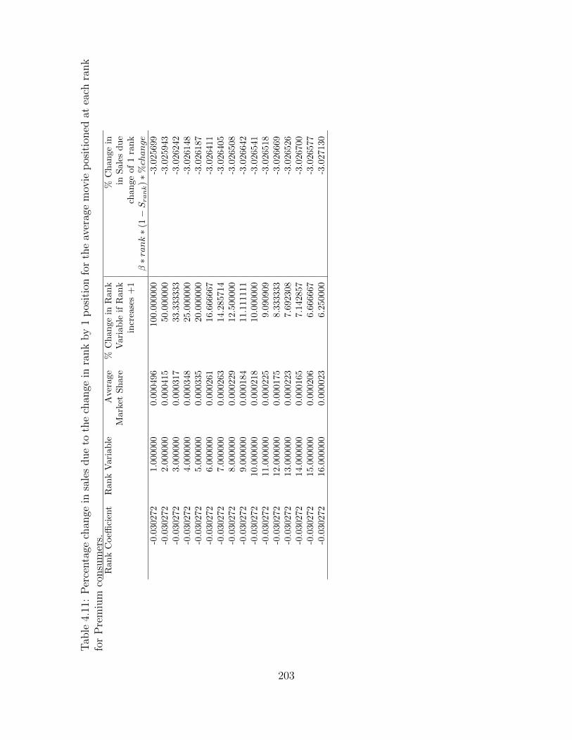
Tab

le4.

11:

Per

centa

gech

ange

insa

les

due

toth

ech

ange

inra

nk

by

1p

osit

ion

for

the

aver

age

mov

iep

osit

ioned

atea

chra

nk

for

Pre

miu

mco

nsu

mer

s.R

ank

Coeffi

cien

tR

ank

Vari

ab

leA

vera

ge

%C

han

ge

inR

an

k%

Ch

an

ge

inM

ark

etSh

are

Vari

ab

leif

Ran

kin

Sale

sd

ue

incr

ease

s+

1ch

an

ge

of

1ra

nk

β∗rank∗

(1−Srank)∗

%change

-0.0

3027

21.0

00000

0.0

00496

100.0

00000

-3.0

25699

-0.0

3027

22.0

00000

0.0

00415

50.0

00000

-3.0

25943

-0.0

3027

23.0

00000

0.0

00317

33.3

33333

-3.0

26242

-0.0

3027

24.0

00000

0.0

00348

25.0

00000

-3.0

26148

-0.0

3027

25.0

00000

0.0

00335

20.0

00000

-3.0

26187

-0.0

3027

26.0

00000

0.0

00261

16.6

66667

-3.0

26411

-0.0

3027

27.0

00000

0.0

00263

14.2

85714

-3.0

26405

-0.0

3027

28.0

00000

0.0

00229

12.5

00000

-3.0

26508

-0.0

3027

29.0

00000

0.0

00184

11.1

11111

-3.0

26642

-0.0

3027

210.0

00000

0.0

00218

10.0

00000

-3.0

26541

-0.0

3027

211.0

00000

0.0

00225

9.0

90909

-3.0

26518

-0.0

3027

212.0

00000

0.0

00175

8.3

33333

-3.0

26669

-0.0

3027

213.0

00000

0.0

00223

7.6

92308

-3.0

26526

-0.0

3027

214.0

00000

0.0

00165

7.1

42857

-3.0

26700

-0.0

3027

215.0

00000

0.0

00206

6.6

66667

-3.0

26577

-0.0

3027

216.0

00000

0.0

00023

6.2

50000

-3.0

27130

203

Tab

le4.

12:

Ow

nra

nk

elas

tici

tyof

dem

and

(β∗x

j∗(

1−Sj))

and

cros

sra

nk

elas

tici

ties

ofdem

and

(β∗x

k∗S

k)

for

Pre

miu

mco

nsu

mer

s.A

ssum

ing

the

mar

ket

shar

eof

the

aver

age

mov

ieat

that

rank

duri

ng

our

exp

erim

ent

12

34

56

78

910

11

12

13

14

15

16

1-0

.03026

0.00003

0.00003

0.00004

0.00005

0.00005

0.00006

0.00006

0.00005

0.00007

0.00008

0.00006

0.00009

0.00007

0.00009

0.00001

20.00002

-0.06052

0.00003

0.00004

0.00005

0.00005

0.00006

0.00006

0.00005

0.00007

0.00008

0.00006

0.00009

0.00007

0.00009

0.00001

30.00002

0.00003

-0.09079

0.00004

0.00005

0.00005

0.00006

0.00006

0.00005

0.00007

0.00008

0.00006

0.00009

0.00007

0.00009

0.00001

40.00002

0.00003

0.00003

-0.12105

0.00005

0.00005

0.00006

0.00006

0.00005

0.00007

0.00008

0.00006

0.00009

0.00007

0.00009

0.00001

50.00002

0.00003

0.00003

0.00004

-0.15131

0.00005

0.00006

0.00006

0.00005

0.00007

0.00008

0.00006

0.00009

0.00007

0.00009

0.00001

60.00002

0.00003

0.00003

0.00004

0.00005

-0.18158

0.00006

0.00006

0.00005

0.00007

0.00008

0.00006

0.00009

0.00007

0.00009

0.00001

70.00002

0.00003

0.00003

0.00004

0.00005

0.00005

-0.21185

0.00006

0.00005

0.00007

0.00008

0.00006

0.00009

0.00007

0.00009

0.00001

80.00002

0.00003

0.00003

0.00004

0.00005

0.00005

0.00006

-0.24212

0.00005

0.00007

0.00008

0.00006

0.00009

0.00007

0.00009

0.00001

90.00002

0.00003

0.00003

0.00004

0.00005

0.00005

0.00006

0.00006

-0.27240

0.00007

0.00008

0.00006

0.00009

0.00007

0.00009

0.00001

10

0.00002

0.00003

0.00003

0.00004

0.00005

0.00005

0.00006

0.00006

0.00005

-0.30265

0.00008

0.00006

0.00009

0.00007

0.00009

0.00001

11

0.00002

0.00003

0.00003

0.00004

0.00005

0.00005

0.00006

0.00006

0.00005

0.00007

-0.33292

0.00006

0.00009

0.00007

0.00009

0.00001

12

0.00002

0.00003

0.00003

0.00004

0.00005

0.00005

0.00006

0.00006

0.00005

0.00007

0.00008

-0.36320

0.00009

0.00007

0.00009

0.00001

13

0.00002

0.00003

0.00003

0.00004

0.00005

0.00005

0.00006

0.00006

0.00005

0.00007

0.00008

0.00006

-0.39345

0.00007

0.00009

0.00001

14

0.00002

0.00003

0.00003

0.00004

0.00005

0.00005

0.00006

0.00006

0.00005

0.00007

0.00008

0.00006

0.00009

-0.42374

0.00009

0.00001

15

0.00002

0.00003

0.00003

0.00004

0.00005

0.00005

0.00006

0.00006

0.00005

0.00007

0.00008

0.00006

0.00009

0.00007

-0.45399

0.00001

16

0.00002

0.00003

0.00003

0.00004

0.00005

0.00005

0.00006

0.00006

0.00005

0.00007

0.00008

0.00006

0.00009

0.00007

0.00009

-0.48434

204

Chapter 5

Conclusion

This thesis covers a theoretical model, an observational study and an experimental study

in the telecommunications and media industries.

In the second chapter of this manuscript we developed a game theoretic model that

predicts the number of infrastructure providers and virtual firms (companies leasing access

from infrastructure providers) that will enter green-field regions. In our model, firm entry

occurs in multiple markets characterized by the demand for a general telecommunication

service and the costs to deploy the appropriate infrastructure to meet demand. The latter

are largely determined by household density.

Using engineering data from publicly available sources and simulation software we de-

veloped, we parameterize the model to analyze several types of regions where NGNs can

be deployed - rural areas, urban areas and downtown areas. We explore how different

wholesale prices can determine the competitive nature and structure of telecommunica-

tions markets and by predicting how many firms are likely to enter each market, our model

205

provides fundamental information for regulators to decide the best type of policy a region

might require to ensure availability of telecommunications service.

We conclude that low wholesale prices can attract a disparate number of virtual providers

to enter the market. The excess competition will reduce the profitability of infrastructure

providers and their incentives to invest. High wholesale prices can deter the entry of virtual

providers and trigger investment. Yet such scenario does not necessarily maximize welfare

which in our simulations can be highest in situations where a single provider invests in

infrastructure opening the network to virtual providers at reasonable prices.

We also confirm the asymmetric business case for the development of NGNs which

motivated the emergence of GSR in the first place: highly populated areas are likely to

develop into competitive telecommunication markets while regions with low household

density will only see very limited investment in network infrastructures and little or no

competition.

Finally, we show that supply side interdependencies among markets, common to the

telecommunications’ industry, make the implementation of GSR non-trivial. We show

that changes in the wholesale price in one market can have undesirable consequences in

the competitive conditions of interrelated regions. Namely we provide an example where

our model predicts that wholesale price changes in a competitive market can have negative

consequences in an interrelated, but less competitive market where the wholesale price was

not changed.

In the third chapter we study the effect of peer influence in the diffusion of the iPhone

3G across a number of communities that were sampled from a large dataset provided by a

206

major European Mobile (EURMO) carrier in one country.

We use community dummies and instrumental variables to control for potential cor-

relation between unobserved subscriber heterogeneity and peer influence. We provided

evidence that the propensity of a subscriber to adopt increases with the percentage of

friends that had already adopted. We estimated that 14% of iPhone 3G adoptions in EU-

RMO were due to peer influence, after controlling for social clustering, gender, previous

adoption of mobile internet data plans, ownership of technologically advanced handsets

and some heterogeneity in the regions where subscribers move during the day and spend

most of their evenings. Our estimate for peer influence without IV is three times lower

that the above statistic, which hints at the fact unobserved effects might be negatively cor-

related with adoption. We provide additional empirical evidence that budget constraints

might be at work and might prevent several family members, or many employees in the

same company, from purchasing the iPhone 3G, which was a conspicuous and expensive

handset for the average consumer in the country studied.

We also provide results from several policy experiments that show that with an effect of

peer influence with this magnitude EURMO would hardly be able to significantly increase

sales by selectively targeting appropriate early adopters to benefit from viral marketing.

We show that a seeding strategy using local degree yields the largest number of additional

adopters among the strategies compared in this paper, but even such a policy could only

hardly break even for the cost/revenue ratio at which the iPhone 3G might have been

commercialized.

In the fourth chapter we design and implement a randomized experiment to determine

207

the role that likes play on the sales of movies over VoD. We use the VoD system of a large

telecommunications provider during half a year in 2012. A new menu in the Highlights

Section of this VoD system was introduced showing the most liked movies in the past few

weeks. Movies with more likes were shown farthest to the left on the TV screen. During

our the experiment, movies were primarily placed in their true rank and shown along with

their true number of likes. At random moments, some movies were swapped and thus

displayed our of order and with a fake number of likes. The movies that were swapped

were selected at random. Randomization allows us to disentangle likes from unobserved

perceived quality and thus estimate the effect of the former on sales.

We found that search costs play a major role on sales. A movie brought from the catalog

into the new menu sells about 7 times more, on average. We found that promoting a movie

by one rank increases weekly sales by 4% on average. We found that a movie promoted

(demoted) to a fake slot sells 15.9% less (27.7% more) than a true movie placed at that

slot, on average across all manipulations we introduced. We showed that this asymmetry

is related to the amount of information publicly available about the movies manipulated.

Better-known movies are less sensitive to manipulations.

We also found that a movie promoted (demoted) to a fake slot receives 33.1% fewer

(30.1% more) likes than a true movie at that slot. Therefore, manipulated movies tend

to move back to their true slot over time This adjustment process is likely to converge

quickly, in a matter of 2 to 3 weeks time, which might lead the provider to promote differ-

208

ent movies over time to obtain increased sales. However, it is not clear whether in the long

run subscribers will believe in the number of likes exhibited at this VoD system if movies

are manipulated often. Another way for the provider to attract attention to, and possibly

increase the sales of, specific movies without manipulating their rank is to strategically

show and hide movies between the Highlights Section and the catalog.

209

210