ESP-r: A Building and Plant Energy Simulation Environment, User ...
63
University of Strathclyde Energy Systems Research Unit 75 Montrose Street Glasgow G1 1XJ, UK Email [email protected] Phone +44 141 548 3986 Fax +44 141 552 8513 University of Strathclyde Energy Systems Research Unit The ESP-r System for Building Energy Simulation User Guide Version 10 Series October 2002 ESRU Manual U02/1
Transcript of ESP-r: A Building and Plant Energy Simulation Environment, User ...

University of StrathclydeEnergy Systems Research Unit75 Montrose StreetGlasgow G1 1XJ, UK
Email [email protected] +44 141 548 3986Fax +44 141 552 8513
University of Strathclyde
Energy Systems Research Unit
The ESP-r Systemfor
Building Energy Simulation
User Guide Version 10 Series
October 2002
ESRU Manual U02/1

Table of Contents
Development history and acknowledgementsAbout this User Guide
Section One: General description of ESP-r1.0 Introduction1.1 Purpose of ESP-r1.2 Structure of ESP-r1.3 Machine environment1.4 System documentation1.5 Further information
Section Two: A guide to effective system use2.0 Introduction2.1 Simulation strategy2.2 General details of program operation2.3 Data file management
Section Three: Exercises3.0 Introduction3.1 List of exercises
Section Four: Example applications4.0 Introduction4.1 Parametric studies4.2 Upgrading strategy4.3 The issue of cost4.4 Innovatory design4.5 Low energy housing4.6 Re-design4.7 Critical control4.8 Feasibility study4.9 Late design-stage use4.10 Comfort4.11 Speculative dev elopment4.12 Training Exemplars4.12.1 Single office4.12.2 Simple building4.12.3 Small house4.12.4 Large house4.12.5 Test cells4.12.6 Special focus4.12.7 Office block4.12.8 Plant
Section Five: Theoretical basis and validity5.0 Introduction5.1 Theoretical basis5.2 Validity5.3 Model value
Appendices
Summary of ESP-r’s Data ModelESP-r Implementation ProceduresGood Practice Guide for ESP-r DevelopersList of ESP-r ReferencesAdding Models to ESP-r
Development history and acknowledgements
The ESP-r system has evolved to its present form over more then two decades. From1974 to 1977 Joe Clarke dev eloped the initial prototype as part of his doctoral research.Then, over the period 1977 to 1980, with funding from the (then) UK Science and Engi-neering Research Council (SERC), ESP-r was refined in a number of respects: the systemwas reorganised and documented, validation trials commenced, multi-zone processingwas implemented and a graphics orientated user interface was established. From 1981through 1986 Professor Clarke was joined by Dr Don McLean and, with further fundingfrom SERC and from the CEC, ESP-r’s capabilities were extended by the addition ofdynamic plant simulation, the inclusion of building air flow modelling, a move to lowcost UnixTM workstation technology and the installation of expert system primitives.
In 1987, the Energy Simulation Research Unit (ESRU) was formed to address the prob-lems confronting the further evolution of building energy and environmental simulation.As part of its research portfolio, ESRU has continued to evolve ESP-r - most notablywithin the framework of the UK Department of Energy’s (now Trade and Industry) Pas-sive Solar Programme, the CEC’s PASSYS project (a 10 member country concertedaction in Passive Solar Architecture), a SERC funded project to establish an intelligentfront-end for the package and within a number of ongoing projects concerned with plantand control simulation. These activities ensured that ESP-r continued to evolve, in termsof further validation, technical extensions and user interface improvements.
Over the past two decades many individuals have made valuable contributions to ESP-rdevelopments. The most important of these have come from our research colleagues atthe University of Strathclyde who have contributed much in the way of computationalmethods and technical support. In particular we are indebted to Tom Maver, Harvey Sus-sock, Alan Bridges, Don Stearn and Iain Forrest (all presently or previously of ABA-CUS). One other colleague springs readily to mind: Damian Mac Randal, now a projectleader within the Informatics Department at the Rutherford Appleton Laboratory. He wasthe driving force behind our move to Unix workstations.
We also extend our thanks to several other individuals: to Fred Winklemann of theLawrence Berkeley Laboratory who helped to develop ESP-r’s time-step control mecha-nism; to Cor Pernot of the FAGO group in Eindhoven who installed ESP-r’s comfort rou-tines and continues to take an active interest in the system; to Jeremy Cockroft, whoworked on the original air flow solver upon which we have built over the years; to DrDechao Tang, Dr Essam Aasem, Dr Abdullatif Nakhi, Dr Cezar Negrao and Dr Tin-taiChow, all formerly PhD students at ESRU, who worked on ESP-r’s plant, moisture flowand CFD algorithms.
At the present time the researchers actively involved in ESP-r developments at ESRUinclude Joe Clarke, Jon Hand, Jan Hensen, Milan Janak, Cameron Johnstone, Nick Kelly,Iain Macdonald, Paul Strachan.

ESP-r User Guide Version 10 Series
About this User Guide
We assume that the user is familiar with some of the more elementary Unix/Linux com-mands and is able to use a Unix/Linux workstation. The main purpose of this User Guideis to introduce a new user of ESP-r to the system and to provide training guidance.
Note that ESP-r has extensive in-built tutorial and help facilities which can be consultedthroughout the system familiarisation process. Detailed information may also be found inESRU’s World-Wide-Web pages <http://www.esru.strath.ac.uk> and in the Appendices tothis User Guide which cover the system’s data requirements, operational details, workedexamples, adding new features to ESP-r, dev elopers good practice guide, implementationprocedure and software structure.
This User Guide only comprises the essential reading material for the first time user ofESP-r, org anised in the following sections:
1 Outline of the system structure and examples of the types of design questions ESP-rcan be used to answer.
2 General guidance on how to make effective use of the system.
3 A series of consecutive exercises allowing the first time user to become familiarwith - and appreciate - the comprehensive features of the system.
4 A number of short case study descriptions illustrating the use of ESP-r in practice.
5 Some information and references on the theoretical basis and validity of the system.

Section OneGeneral description of ESP-r
and itsassociated documentation
Contents
1.0 Introduction
1.1 Purpose of ESP-r
1.2 Structure of ESP-r
1.3 Machine environment
1.4 System documentation
1.5 Further information
ESP-r User Guide Version 10 Series 1-2
1.0 Introduction
This first section of the User Guide gives a general overview of ESP-r (EnvironmentalSystems Performance; r for "research"); a computing environment for building and/orplant energy simulation. The application potential of ESP-r is outlined by citing sometypical design questions which the model has been used to answer. Then, the programmodules which comprise the system are outlined, along with the essential hardware envi-ronment. Finally, some further information sources are indicated.
ESP-r is the outcome of model development projects funded over the years by the UKScience and Engineering Research Council (now EPSRC) and the European Commis-sion’s DGXII. Significant contributions have also been made by many individuals as out-lined in the Development history and acknowledgements section.
ESP-r is free software. It is released under the GNU General Public License.
1.1 Purpose of ESP-r
ESP-r is a transient energy simulation system which is capable of modelling the energyand fluid flows within combined building and plant systems when constrained to conformto control action. The package comprises a number of interrelating program modulesaddressing project management, simulation, results recovery and display, database man-agement and report writing.
One or more zones within a building are defined in terms of geometry, construction andusage profiles. These zones are then inter-locked to form a building, in whole or in part,and, optionally, the leakage distribution is defined to enable air flow simulation. Theplant network is then defined by connecting individual components. And, finally, themulti-zone building and multi-component plant are connected and subjected to simulationprocessing against user-defined control. The entire data preparation exercise is achievedinteractively, and with the aid of pre-existing databases which contain standard (or user-defined) constructions, event profiles and plant components. Additional modules exist topermit an increase in simulation rigour if the related data is available.
A central Project Manager allows importing/ exporting of building geometry from/ toCAD packages and other specialised simulation environments such as Radiance for light-ing simulation.
ESP-r is equally applicable to existing buildings and new designs, with or withoutadvanced technological features. The system offers sophisticated input/output facilitieswhich enable the user to answer such design questions as
• What, and when, are the peak building or plant loads and what are the rank-orderedcausal energy flows?
• What will be the effect of some design change, such as increasing wall insulation,altering the window shape and size, changing the glazing type or distribution, intro-ducing daylight control devices, re-zoning the building, re-configuring the plant orchanging the heating/ cooling control regime?
• What is the optimum plant start time or the most effective algorithm for weatheranticipation?

ESP-r User Guide Version 10 Series 1-3
• How will comfort levels vary throughout the building?
• What benefits can be expected from the different possible lighting control strate-gies?
• What are the relative merits of different heating and cooling systems and their asso-ciated controls?
• How will temperature stratification, in terms of zone sensor and terminal unit loca-tion, affect energy consumption and comfort control?
• What contribution does building infiltration and zone-coupled air flow make to thetotal boiler or chiller load and how can this be minimised?
• How do suggested design alterations affect air flow and fresh air distribution (i.e.indoor air quality) within the building?
• What is the effect of special glazings (such as thermotropic, holographic, low-e orelectrochromic glazing) on summer overheating?
• Which are the benefits from architectural building features such as atria, sunspaces,courtyards, etc?
• What is the contribution (in terms of energy saving and thermal comfort) of a rangeof passive solar (heating or cooling) features?
• What is the optimum arrangement of constructional elements to encourage goodload levelling and hence efficient plant operation?
• What are the energy consequences of non-compliance with prescriptive energy reg-ulations or, conversely, how should a design be modified to come within somedeemed-to-satisfy performance target?
• Which heat recovery system performs best under a range of typical operating con-ditions?
and so on. This allows the user to understand better the interrelation between design andperformance parameters, to then identify potential problem areas, and so implement andtest appropriate building, plant and/or control modifications. The design to result is moreenergy conscious with better comfort levels attained throughout.
1.2 Structure of ESP-r
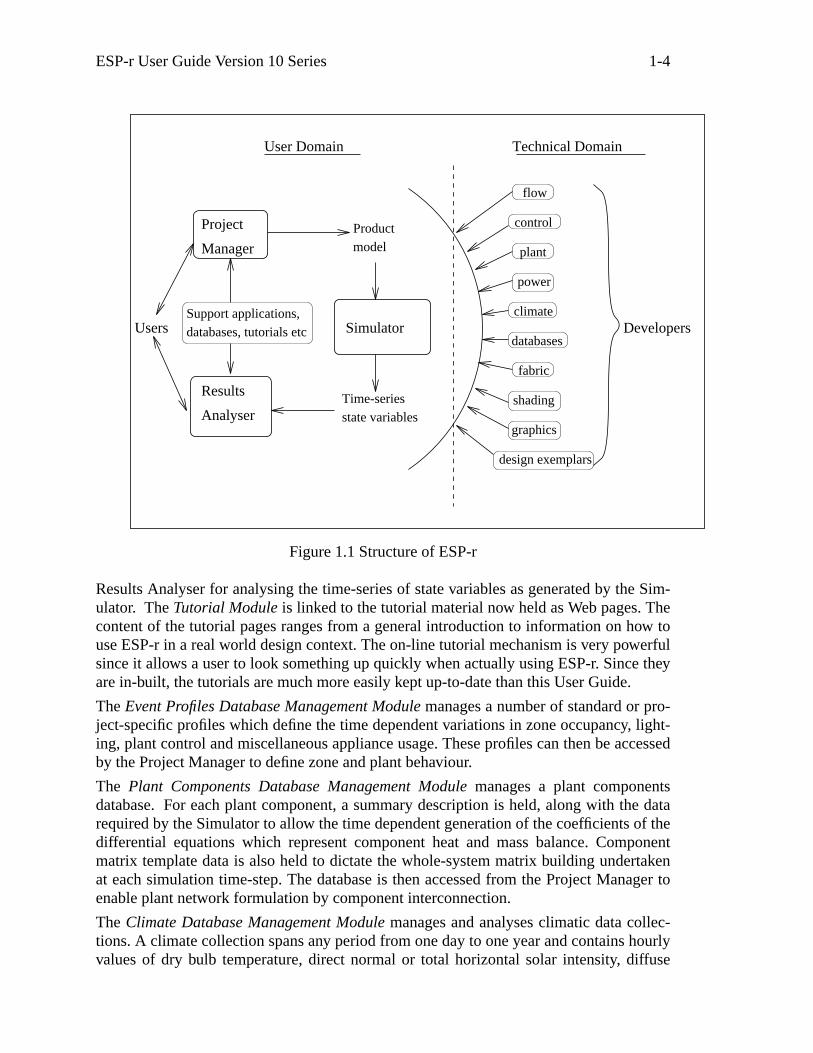
Figure 1.1 shows the relationship between the program and database modules which formthe simulation environment. In this User Guide only the Users-side of the environmentwill be addressed.
The Project Manager allows the interactive definition of some building and plant configu-ration which is to be subjected to some weather influence and simulated over time. Thecomplete description of the building and plant configuration is called the product model.All data items, as input, are subjected to strict range and legality checks before beingdirected to disk file for later recall. To ease the input burden, the user is given access tostandard databases so that constructions, event profiles and plant components can beaccessed by name or simple code number reference. Also, many input items have a corre-sponding default value so that typed responses can vary as a function of the design infor-mation to hand at any time during a design’s evolution. The Project Manager also con-trols user access to the other ESP-r programs such as the Simulator for simulation and the
ESP-r User Guide Version 10 Series 1-4
Manager
Project
Support applications,databases, tutorials etc
Results
Analyser
Simulator
Time-seriesstate variables
modelProduct
flow
control
power
plant
databases
climate
fabric
shading
graphics
design exemplars
Users Developers
User Domain Technical Domain
Figure 1.1 Structure of ESP-r
Results Analyser for analysing the time-series of state variables as generated by the Sim-ulator. The Tutorial Module is linked to the tutorial material now held as Web pages. Thecontent of the tutorial pages ranges from a general introduction to information on how touse ESP-r in a real world design context. The on-line tutorial mechanism is very powerfulsince it allows a user to look something up quickly when actually using ESP-r. Since theyare in-built, the tutorials are much more easily kept up-to-date than this User Guide.
The Event Profiles Database Management Module manages a number of standard or pro-ject-specific profiles which define the time dependent variations in zone occupancy, light-ing, plant control and miscellaneous appliance usage. These profiles can then be accessedby the Project Manager to define zone and plant behaviour.
The Plant Components Database Management Module manages a plant componentsdatabase. For each plant component, a summary description is held, along with the datarequired by the Simulator to allow the time dependent generation of the coefficients of thedifferential equations which represent component heat and mass balance. Componentmatrix template data is also held to dictate the whole-system matrix building undertakenat each simulation time-step. The database is then accessed from the Project Manager toenable plant network formulation by component interconnection.
The Climate Database Management Module manages and analyses climatic data collec-tions. A climate collection spans any period from one day to one year and contains hourlyvalues of dry bulb temperature, direct normal or total horizontal solar intensity, diffuse
ESP-r User Guide Version 10 Series 1-5
horizontal solar intensity, wind speed, wind direction and relative humidity. The climatemanagement module offers solar radiation prediction, curve fitting to daily maximum andminimum data, statistical analysis, graphical and tabular display and general data man-agement. The climate data is required by the Simulator to generate the time dependentboundary conditions for the building and plant configuration.
The Simulator is the building and plant simulation engine which predicts building andplant energy/ fluid flows by a rigorous numerical method. The building/ plant network isdivided into a large number of finite volumes. Then, at each time-step as a simulationproceeds, an energy and mass balance is applied for all volumes, giving rise to a differen-tial matrix for the entire system. This is then solved by custom matrix processing soft-ware in terms of any user-imposed control objectives.
The Results Analysis Module operates on the simulation results located in a database bythe Simulator. A variety of output options are available: perspective visualisations,results interrogation, statistical analysis, graphical display, tabulations, frequency binningand 3D plotting.
The Insolation and Shading Module is a support module which predicts the time-seriesshading of external zone surfaces (opaque and transparent) as caused by facade and siteobstructions and/or the time-series insolation of internal zone surfaces (opaque and trans-parent) as caused by solar penetration through windows. The predictions for any surfacecan, optionally, be archived in a shading/insolation database for access and use within asimulation.
The View Factors Module computes the black body view factors between each zone sur-face pairing for use by the Simulator to evaluate internal longwav e radiative exchanges. Italso evaluates zone comfort level variations.
Building/ plant fluid flow simulation can be performed by the Simulator in tandem withthe heat balance calculations. In this case full account will be taken of buoyancy drivenair movements between outside and inside and between internal zones. If pressure drivenair flow dominates, it is possible to use the Flows Simulation Module in stand-alone modeto predict infiltration and zone-coupled air flow. Buoyancy effects are still included butcorrespond to fixed zone temperatures assigned by the user.
The Construction Data Management Module manages (creates, modifies, edits and lists)primitive and composite constructions databases. The materials database contains thethermophysical properties of conductivity, density, specific heat, solar absorptivity andemissivity for a number of standard homogeneous elements. Diffusion resistance factorsare also held as required by ESP-r’s interstitial condensation computations. A second,project-related database can also be created to hold multilayered constructions formedfrom elements extracted from the materials’ database. Both databases can then beaccessed from the Project Manager as required.
A number of ESP-r modules create and/or manipulate random access, binary disk filessuch as the constructions databases, the event profiles database, and the simulation resultsdatabase. They also allow for the transformation of ESP-r’s binary files to ASCII formatand vice versa. This permits the transmission of binary databases to other computer sites(via tape for example) and, if a user is experienced, direct file editing.

ESP-r User Guide Version 10 Series 1-6
In normal use, the three main modules, the Project Manager, the Simulator and theResults Analyser, are used to investigate building and/or plant performance and, by itera-tion, to assess the consequences of any change to system design or control. The databasemodules help to reduce the input burden and the support modules exist to allow the sub-system they address to be treated with greater rigour, if this can be justified by the designobjectives and data to hand.
The theories underlying ESP-r and the validity of the Simulator are summarised in Sec-tion 5 and presented, in detail, in the following references:
• Clarke J A Energy Simulation in Building Design, 2nd Edition, Butterworth-Heine-mann, Oxford, 2001.
• Tang D Modelling of Heating and Air-Conditioning Systems, PhD Thesis, Univer-sity of Strathclyde, 1985.
• Hensen J L M On the Thermal Interaction of Building Structure and Heating andVentilating System, PhD Thesis, University of Eindhoven, 1991.
• Aasem E O Practical Simulation of Buildings and AIr-Conditioning Systems in theTr ansient Domain, PhD Thesis, University of Strathclyde, 1993.
• Negrao C O R Conflation of Computational Fluid Dynamics and Building ThermalSimulation, PhD Thesis, University of Strathclyde, 1995.
• Nakhi A E Adaptive Construction Modelling Within Whole Building Dynamic Sim-ulation, PhD Thesis, University of Strathclyde, 1995.
• Chow T T Air-Conditioning Plant Component Taxonomy by Primitive Parts, PhDThesis, University of Strathclyde, 1995.
• MacQueen J The Modelling and Simulation of Energy Management Control Sys-tems, PhD Thesis, University of Strathclyde, 1997.
• Kelly N J Towards a Design Environment for Building-Integrated Energy Systems:The Integration of Electrical Power Flow Modelling with Building Simulation, PhDThesis, University of Strathclyde, 1998.
• Hand J W Removing Barriers to the Use of Simulation in the Building Design Pro-fessions, PhD Thesis University of Strathclyde, 1998.
• Beausoleil-Morrison I The Adaptive Coupling of Heat and Air Flow ModellingWithin Dynamic Whole-Building Simulation PhD Thesis, University of Strathclyde,2000.
1.3 Machine environment
ESP-r requires the following hardware and software:
• A UNIXTM or LINUX workstation# offering X-Windows and with at least 128MBytes RAM. Implementations exist for SUN, Silicon Graphics and Linux (PCand Mac) platforms.
• A disk capacity to store the executables, manuals, tutorials, training examples (˜25MBytes), perhaps source code (˜20 MBytes) and simulation results (˜2 MBytes perzone-year at a one hour time step).

ESP-r User Guide Version 10 Series 1-7
• Fortran77 and C compilers.
• A laser writer for graphical hard copy.
1.4 System documentation
In terms of usage, this User Guide and the web-based tutorial facilities of ESP-r are themain sources of documentation. In addition, a number of papers concerning ESP-r devel-opment and application can be found in the literature. A full list of publications can befound on the ESRU web site.
As indicated in the Table of Contents, the User Guide has a number of appendices. Theseare available from our FTP server: they can be automatically downloaded by accessingESRU’s publication list on the WWW (http://www.esru.strath.ac.uk/) or by direct ftp (filetransfer protocol) transfer. In the latter case, ftp to ftp.strath.ac.uk and login as anony-mous with your email address as the password. The documents will be found in directoryEsru_public/documents.
Papers and technical reports cover issues such as:
• How to add new entities such as climate data, project-specific constructiondatabases and plant components.
• A list of training assignments enabling an instructor to assess whether the trainingmaterial is absorbed properly, and enabling the trainee to check whether the train-ing material is understood.
• Good practice guidelines for researchers interested in developing or expandingparts of ESP-r.
• A bibliography describing much of ESP-r’s technical detail and philosophy. Thislist includes books, journal articles, conference papers and internal ESRU reports.In some cases PostScript or pdf versions of these publications are available.
• A summary of the tasks to be undertaken when implementing ESP-r at a particularsite.
• A summary of ESP-r’s underlying data model.
• Some step-by-step worked examples of simulation projects.
1.5 Further information
ESP-r is released under the terms of the GNU General Public License. It can be used forcommercial or non-commercial work subject to the terms of this open source licenceagreement.
Although ESP-r can be used for free, it is often the case that a new ESP-r site will incur anominal expense. For example it may be appropriate to send someone to one of the ESP-r courses which we organise regularly at ESRU (the cost is approximately £500 per per-son). We strongly recommend this course of action for all new users to ensure that thelearning process is as short and painless as possible. Dates of forthcoming courses arelisted on the ESRU web site. In addtion, ESRU offer a range of options for supporting theuse of ESP-r in organisations. Contact ESRU for details.
ESP-r can be downloaded from the web site http://www.esru.strath.ac.uk by following theappropriate links to the software. Note that, because ESP-r is under active dev elopment at

ESP-r User Guide Version 10 Series 1-8
a growing number of sites, there are frequent updates and revisions.
ESP-r is a building and plant energy simulation environment which is under developmentat various research centres throughout Europe and elsewhere. These developmentsinvolve both enhancements and new dev elopments to the existing system as well as vali-dation activities and application related research.
The people working with ESP-r keep in contact via an electronic communication plat-form. The purpose of this is to keep each other informed about ongoing and planneddevelopments, system related publications, new results, emerged problems, upcomingreleases, etc. To join, simply email the string "subscribe esp-r <your email address" [email protected]. After your name has been registered, you can communicatewith other subscribers by sending messages to [email protected]. Please note that anye-mail messages received by the virtual user [email protected] will be forwardedunmoderated to all people currently subscribed.
Further technical, operational or commercial details on ESP-r may be obtained fromESRU at the address on the front of this User Guide. Alternatively, you may want tobrowse through our web pages, which can be accessed from http://www.esru.strath.ac.uk.

Section TwoA guide to effective system use
Contents
2.0 Introduction
2.1 Simulation strategy
2.2 General outline of program operation
2.3 Data file management

ESP-r User Guide Version 10 Series 2-2
2.0 Introduction
In use ESP-r can be divided into two distinct parts.
The first is concerned with establishing a valid data model (description of the buildingand/or plant configuration) for simulation. This will involve the use of the Project Man-ager. The support modules can then be used to increase the detail of the simulation to fol-low, if this is deemed necessary.
The second part is concerned with the simulation processing and subsequent results anal-ysis. This will involve the use of the Simulator and the Results Analyser. Note that allESP-r modules are invoked from the Project Manager.
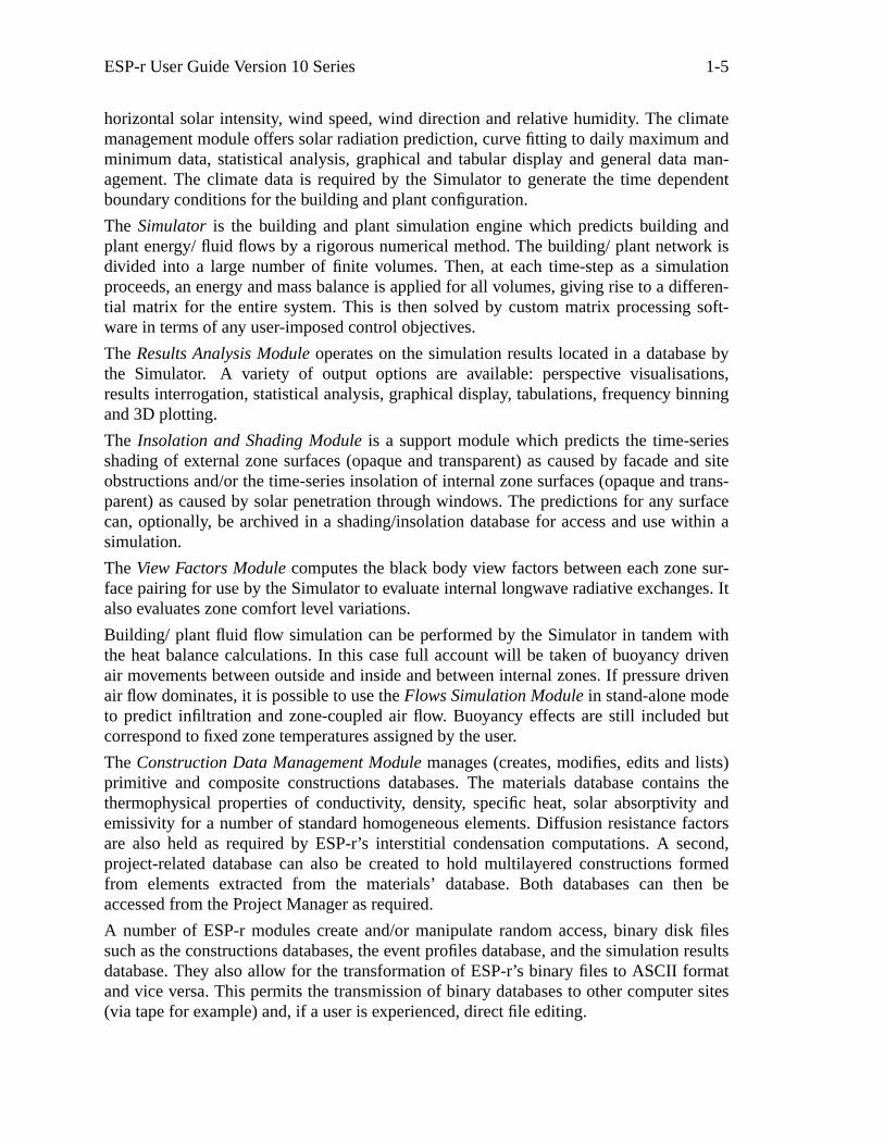
In using ESP-r it is not important to know all the relationships between the ESP-r pro-gram modules and the system’s data structures. However for a deeper appreciation theserelationships are shown in Figure 2.1.To work with ESP-r you need to be able to cope with a range of technical concepts relat-ing to material properties, control systems, and the like. Information on the data require-ments of ESP-r is held on-line and is accessible through the Project Manager (via its tuto-rial facility). Additional details are given in a separate document "Summary of ESP-r’sData Model".
For each zone in the building a geometry, construction and operations file must be estab-lished. Then, optionally and to increase simulation rigour, one or more of the followingzone files can be set up to replace the default schemes implied by the data of the essentialfiles: a shading/insolation file, a blind/shutter control file, a view factor file, an air flowfile, a casual gain (control) file and a convection coefficients file. The existence of theseoptional files is indicated by the entries of a zone utilities file created for the purpose.The system configuration file is now set up to define the zones and, perhaps, the plantcomponents which will participate in a simulation. Following this, the configuration con-trol file is established to define the control to be imposed on building zones and plantcomponents. All of these files are created and/or edited via the Project Manager. Thisprogram module can also be used to establish the data sets as required by the Fluid FlowSimulation Module and the Insolation and Shading Prediction Module; namely, a config-uration leakage distribution file, a pressure coefficients file and a site obstructions file.Note that some of the optional zone files can also be created directly from the supportmodules - for example the View Factor Prediction Module can create a zone view factorfile. This is a powerful feature of ESP-r.
There are other files active in the system. These include the primitives and compositeconstruction databases, the event profiles database, the plant components database, thewindows database and the climate database. In addition: the Simulator will produce twodatabases, for building- and plant-side, for transmission to the Results Analyser; the Sim-ulator can also produce a fluid flow results file for analysis and archival purposes; andmany of the modules can produce detailed computation trace files for fault finding andhighly focused appraisals. Figure 2.1 summarises these possibilities and indicates the filetypes involved.
The next section of the documentation set outlines a strategy for effective use of thesemodules. Interactive operation, by means of hierarchical menu drivers or function buttonprotocols, is also explained and advice is given on managing the file structures whichresult from the data preparation and simulation activities.

ESP-r User Guide Version 10 Series 2-3
prj: project management facility
bps: simulation ‘engine’
res: results recovery and analysis
mrt: inter-surface view factor & mrt calcs.
tdf: temporal definitions db management
cfg: problem topology checking utility
* interactive definition of building plant and flow networks* full data checking and editing options* central desktop for controlling problem definition facilities, support utilities, simulations and results recovery
* processing of combined building/ plant/mass flow domains* variable period and timestep control* imposition of complex control regimes* simultaneous energy & mass balance
* support for exploring performance via causal energy chaining at zones and surfaces* time-step tabulations of variables* summary of variables* graphical display* statistical analysis* comfort analysis
pro: event profiles db management
pdb: plant component db management
clm: climate db analysis & management
ish: external shading and internal insolation prediction
temporal definitions db
shading / insolation db
primitive constructions db
multilayer constructions db
event profiles db
plant components db
optical properties db
climatic time-series db
pdf: plant network definitions
mfs: stand-alone mass flow solver & results recovery
problem description
mass flow resultsresults database
3rd party graphing & analysis packages
information flow
application control
3rd partyCAD
export
applications
databases
Figure 2.1 Relationship between the ESP-r application modules and databases.
2.1 Simulation strategy
The following step-by-step procedure should be closely followed by a novice. On theother hand, an experienced user may prefer an alternative strategy which bypasses somesteps or changes their order.
1. Analyse the design problem in hand and decide on the performance features to beappraised by ESP-r. Perhaps zone comfort levels are to be determined, the conse-quences of alternative design options assessed, or an optimum control regime for-mulated. This is an important task since it will influence the time and expenseincurred thereafter.
ESP-r User Guide Version 10 Series 2-4
2. Now decide on the minimum number of building zones and plant componentswhich will yield the performance measures required. For example, a one zonebuilding model will allow an appraisal of summer overheating in the absence ofcooling and against any number of design hypotheses. The same model, combinedwith a six plant component air conditioning plant (a mixing box, humidifier, fan,cooler, heater and supply duct, say), will allow a study of plant energy consumptionagainst several control options. Av oid, in the first instance, any attempt to simulatelarge, complex building/plant systems. It is, of course, possible to undertake suchan exercise, but only at the expense of time (data preparation) and cost (simula-tion). Very often good design insight can be obtained from simulations directed atportions of the overall system. It is important not to be merely led by the systembut to giv e careful thought to the problem composition. Perhaps small multi-zonebuilding problems, with specified zone conditions maintained, can be used to studyseveral building design options. Then, at some later stage, a plant systems can beprogressively added. In ESP-r terminology, the final system for simulation, irre-spective of size or composition, is termed the system configuration.
3. A computer model of the system configuration must now be created via the ProjectManager. The underlying procedure is as follows. Firstly, each building zone in theconfiguration is described in terms of its geometry, construction and operation.This results in the creation of three mandatory disk files per zone. A system config-uration file is then built. This contains a reference to these zone files, informationdefining zone interaction, and a description of the plant network (if one exists) interms of individual components, their inter-connections and building associations.At the appropriate point, any of the constructions databases, the event profilesdatabase, the plant components database or the optics database can be accessed andan item contained therein extracted to define a zone property or plant component.
The designer is simply required to answer a series of questions concerning the sys-tem configuration. Control of this interactive dialogue, along with validity checkingand automatic disk file building, is the principal function of the Project Manager.
4. At this stage, additional model details can be added.
An air flow file containing time-series infiltration and zone-coupled air flow for useduring a simulation. If present, these air flows supersede the design air change pro-files specified in the corresponding zone operation file. Note that if a building leak-age description is active (see later) then calculated flows will supersede both designair change profiles and time-series air flow data.
A casual gains file containing time-series heat gains for use during a simulation.Again, if specified, the casual gains will supersede any casual gain profiles definedin the corresponding zone operation file.
A casual gains control file containing information on scheduling of casual gains inorder to simulate, for example, various switching strategies for artificial lightingbased on the availability of daylight.
A view factor file containing inter-surface view factors for use in a simulation toimprove longwav e radiation calculations.

ESP-r User Guide Version 10 Series 2-5
A shading/insolation file containing time-series data on external surface shadingand/or internal surface insolation.
A convection coefficients file allowing the specification of zone surface convectionvalues to supersede those values which are computed at simulation time on thebasis of natural convection considerations.
A transparent multi-layered constructions file allowing elected zone multi-layeredconstructions to be declared transparent.
A flow domain file specifying a 1-, 2- or 3-D grid and related parameters in supportof a CFD simulation.
Each of these optional zone files can be created by terminal input directed by theProject Manager.
The time taken to reach this stage can vary greatly. An experienced user willrequire about 20 minutes per zone if the required data is readily available. On theother hand a beginner can take substantially longer. The only rule is to omit com-plexity in cases where its inclusion cannot significantly influence the performanceaspect to be tested. For example, the omission of wall vapour barriers will have lit-tle effect on summer cooling loads but will completely alter winter interstitial con-densation profiles.
5. A plant network can now be defined, component-by-component, and connected tothe established building model. It is normal practice to bypass this step at an earlydesign stage. Instead ideal control statements are associated with each zone toallow a study of the effects of the various design parameters. At some later timethe plant is added to allow a study of the control issues. Of course, if the relation-ship between the building-side design issues and the plant characteristics arestrong, and the plant details are known, then a combined building/plant study canbe undertaken from the outset.
6. Simulations can now be commissioned from within the Project Manager against theassumption that the configuration is not subjected to control (a free-floating simula-tion). However, in most cases, some control will be required. From the ProjectManager the control regime can be specified in terms of sensors, actuators and con-trol laws. The control specification is stored in the configuration control file whichis then invoked from the Simulator. This configuration control file, together withthe system configuration file (which references the basic zone files and the activeplant components), and a climate file are the only files required by the Simulator tocompletely describe the problem for simulation processing.
7. If air flow within the building configuration is to be simulated by the Simulator intandem with the energy simulation (and perhaps a zone CFD simulation), it is nec-essary to define the distributed building leakage and to ensure that the requiredpressure coefficient sets are located in a related database. Both operations aredirected by the Project Manager, resulting in two further disk files: the fluid flownetwork and pressure coefficients files. The names of these files are given to theSimulator at the time of configuration file creation. The Simulator will now assessthe pressure and temperature driven air flows for the defined zones and disregardany air change profiles (located in the corresponding zone operations file) or active

ESP-r User Guide Version 10 Series 2-6
zone air flow file.
8. From within the Project Manager it is possible to check configuration geometry bycomputing area and volume quantities or by generating perspective displays. Atthis stage, it is possible to create a description of surrounding site obstructions todefine the objects which will cause target zone shading.
Throughout the entire data preparation process, the Project Manager offers editingand listing operations so that mistakes can be easily rectified and hard copy recordscan be kept.
9. The climate analysis module can now be used to analyse the climatic collectionsheld on disk in the format required by ESP-r. By this mechanism, one collection isselected, and typical sequences identified, to provide boundary conditions whichbest stress the performance attribute to be tested.
10. Simulations are now performed from within the Project Manager against one ormore system configuration and configuration control files. Changing either of thesefiles, or the climate file, allows different design options and control regimes to betested under different weather influences.
11. All results recovery and analysis is then undertaken with the help of the ResultsAnalyser (invocable from within the Project Manager), with the principal objectiveof understanding the cause and effect relationships implied by the energy flowpathmagnitudes and directions.
12. Appropriate design modification can now be implemented via the Project Managerby editing a mandatory or optional zone file, the system configuration file or theconfiguration control file. In this way constructions can be changed, operationalschemes modified, plant layout re-configured, shading devices added or removed,and so on.
2.2 General outline of program operation
A session with ESP-r might adhere to the following sequence.
• Log on to the computer offering ESP-r.
• Start ESP-r by issuing the command esp-r. This will start ESP-r in its defaultgraphics mode. You can specify an alternative mode from the following list:
esp-r -mode text (text only mode with no pauses)esp-r -mode graphic (default)
It is also possible to start up ESP-r directly with a configuration file. For exampleesp-r -file xxx.cfg will start ESP-r with the problem specified in the system configu-ration file xxx.cfg already loaded into the Project Manager.
The start-up window size can also be controlled: type esp-r -help for the requiredsyntax.
• Select commands as required from the menus displayed and thereby pick a paththrough the program.
• Answer the questions posed at each interaction.
• Eventually terminate the program by returning to the main menu and selecting theExit command.

ESP-r User Guide Version 10 Series 2-7
• Delete any unwanted files; for example, zone files no longer required or results files(usually large) which have been fully analysed.
• Log off after checking that any disk quotas have not been exceeded.
All program menus are hierarchical so that each menu pick will result in a particular pro-cessing option (with control returning to the same menu level), or will lead to a lowerlevel command menu. In graphics mode, menu picks are initiated by the left mouse but-ton. In text mode selection is by an identifier.
To questions requiring a yes/no response a user may type 1, Y, y, YES or yes and 0, N, n,NO or no. Also, after some output sequences, the program will pause to allow examina-tion of the displayed page. The pause state is indicated by a more button at the bottomscreen position. To continue click the left mouse button over the "more" button.
2.3 Data file management
In addition to the database structures essential to ESP-r’s operation (containing primitiveand composite constructions, event profiles, plant components and climatic collections),the following file types may be produced in a typical session.
• A mandatory geometry, construction and operation file for each zone.
• An optional air flow, casual gains, shading/insulation, view factor, surface convec-tion and transparent multi-layered construction file for some or all zones.
• A mandatory system configuration file and, perhaps, a configuration control file.
• Optionally, a fluid flow network description file (i.e. a leakage distribution file inthe case of a building air flow network), a pressure coefficients file and a fluid flowresults file (i.e. air flow results in the case of an air-only flows problem).
• One or more simulation results files.
File Type ExtensionSystem Configuration .cfgConnections .cnnSystem Control .ctlGeometry .geoConstruction .conOperations .oprShading/Insolation .shdView Factors .vwfAir Flows .airConvection Coefficients .hcfSite Obstructions .obsMass Flow Network .mfnTransparent Constructions .tmcCasual Gains Control .cgcCFD file .dfd
Table 2.1 Filename convention

ESP-r User Guide Version 10 Series 2-8
Effective file management can only follow from a file naming convention (largely auto-mated by the Project Manager) in which the name itself yields information about the pro-ject and file type. In ESP-r the file type is reflected in the filename extension as indicatedin Table 2.1.
Remember to avoid unnecessary complexity by keeping the systemconfiguration as simple as allowed by the design issue being studied.

Section ThreeExercises
Contents
3.0 Introduction3.1 List of exercises

ESP-r User Guide Version 10 Series 3-2
3.0 Introduction
There a number of simulation tools available for energy efficient building design,ranging from simplified tools to detailed simulation programs. Several of these aredescribed on Web pages that can be found via the Web address given later in this section.To learn the capability of such design tools, it is useful to study:
a) the types of analysis questions that they can address and the benefits of usingenergy and environmental simulation;
b) how to use the tools; and
c) the underlying theory upon which the numerical processing and analysis functionsof the tools are based.
The exercises and assignments described in this section are concerned with how touse one particular detailed simulation program, ESP-r, but those following the course areencouraged to also refer to related Web-based material.
In order to be able to use ESP-r and to appreciate the following sections, it isassumed that you have access to a Unix workstation (you will need a personal useraccount on the machine) and that you have a number of basic computer skills. A numberof exercises have been designed to progress ESP-r users from the category of novice tospecialist over a period of time which will depend on the individual’s aptitude andstamina. Once a level of proficiency has been attained, the exercises of section 4 can beattempted.
With the exercises are ten assignments which gradually increase in difficulty. It issuggested that the course participant follows the exercises and assignments in the ordergiven. The assignments serve a dual purpose. They enable the instructor to assesswhether or not the training material is being absorbed effectively. For the course partici-pant they form a series of "real world" consultancy sub-tasks enabling the participant tocheck whether the training material is understood, while at the same time placing ESP-rin a realistic context. Each assignment has an associated prerequisite exercise, such aslearning email in the case of assignment 1. The outcome of each assignment should besent by electronic mail to the supervisor.
The exercises and assignments can be accessed by a Web browser, and it is sug-gested that they are constantly displayed in one window as the course participant pro-gresses through the course.
The relevant Web address is:
http://www.esru.strath.ac.uk
The course participant should follow links from this high level page to ESP-r trainingcourses and from there to the structured exercises.

ESP-r User Guide Version 10 Series 3-3
3.1 List of Exercises
Foundation level exercises
1 Getting started on the workstation2 Configuring the workstation for ESP-r use3 Overview of ESP-r4 Exploring the in-built training exemplars5 Defining a problem to ESP-r - the basics6 Simulation - the basics7 Results analysis - the basics8 Problem definition - databases9 Problem definition - geometry10 Problem definition - constructions11 Problem description - operations12 Problem definition - inter-zone connections13 Climate data and its analysis14 Control capabilities15 Simulation - advanced facilities16 Results analysis - additional facilities17 Review of files and program modules18 Review of progress
Intermediate level exercises
19 Shading and insolation analysis20 Fluid flow analysis21 Plant and control modelling22 Lighting analysis23 Other ESP-r facilities24 Upcoming features
Expert level exercises
25 Making Models: CAD and Attribution26 Making Models: Fluid Flow, Plant and Control Networks27 Making Models: Enhanced Resolution28 Integrated Performance Appraisal29 Edit/ compile/ link test cycle

Section FourExample applications
of theESP-r system
Contents
4.0 Introduction4.1 Parametric studies4.2 Upgrading strategy4.3 The issue of cost4.4 Inovatory design4.5 Low energy housing4.6 Re-design4.7 Critical control4.8 Feasibility study4.9 Late design-stage use4.10 Comfort4.11 Speculative dev elopment4.12 Training exemplars4.12.1 Single office4.12.2 Simple building4.12.3 Small house4.12.4 Large house4.12.5 Test cells4.12.6 Special focus4.12.7 Office block4.12.8 Plant

ESP-r User Guide Version 10 Series 4-2
4.0 Introduction
Sections 4.1 through 4.11 presents a number of short case studies of typical and atypicaldesigns as analysed by ESP-r. They hav e been selected to indicate the possibilities forperformance assessment by simulation. The remaining sections describe a number ofsimulation exercises based on exemplars supplied with the system. These have a dualrole: to test the ESP-r program modules on first implementation and to provide trainingfor new users thereafter. The exercises progress from the simple to the more complex andhave been designed to test several aspects of ESP-r. Each of the training sessions dealswith a basic problem type with variations which explore simulation topics.
Throughout the exercises reference is made to standard ESP-r databases and test files. Asexplained elsewhere, such files are held in a strict directory structure. In the text that fol-lows the Unix syntax is used so that ˜esru/esp-r/climate means sub-directory climate ofsub-directory esp-r of the home directory (wherever defined) of esru. Similarly ˜esru/esp-r/training/office means sub-directory office of sub-directory training of sub_directory esp-r of the home directory of esru.
4.1 Parametric studies
Parametric analysis of building energy performance is, perhaps, the prerequisite of a morecomplete understanding of the issues relating to energy efficient building design. The pro-cess of simulation can be used to increase the corpus of knowledge upon which futuredesigns can be built. ESP-r has been used as the simulation tool in a number of paramet-ric studies.
In one, different window designs were analysed in terms of their performance in Britishand Scandinavian climates. Annual simulations were performed for a number of combi-nations of facade orientation, window size, window type and fabric capacity sampledfrom the many combinatorial possibilities. Typical occupancy patterns, internal gains andwindow curtain operation was assumed throughout. The different windows were thenanalysed in terms of the cost-benefit associated with the provision of varying comfortstandards.
In another study, the model was used to generate design guidelines in public buildings bysystematically varying the major design parameters such as insulation, capacity, windowsize, heating system regulation and degree of air permeability.
4.2 Upgrading strategy
Many Government agencies in the UK own housing stock which dates from the early1950’s. In recent times much of this stock has fallen due for upgrading. Obviously somemechanism must be employed to establish the most productive strategy. ESP-r has beenused as such a mechanism.
A sample of houses in any estate are analysed, firstly in their original form, and subse-quently with a range of alternative upgrading features formulated on the basis of the ini-tial simulation results. In one case, the prime heat loss path was identified by ESP-r asbeing through the suspended timber floor. This occurred in a building for which substan-tial wall insulation was planned. As a result the upgrading proposal was modified and theclient’s inv estment put to better use.
ESP-r User Guide Version 10 Series 4-3
4.3 The issue of cost
ESP-r was once used by a large regional council to investigate the possibilities in a pro-posed building conversion. The study involved an in-depth investigation into heatingdemand diversity as affected by alternative zoning strategies, plant control schedules andfabric treatments. Their resulting report included the technical details of the project butwent on to raise the following general points.
• The total cost incurred by them in the simulation exercise was calculated at half thecost incurred in a parallel exercise which involved only the calculation of zone heatloss by conventional ‘manual’ methods.
• The results from the ESP-r exercise allowed a more detailed analysis of both thebuilding and plant performance than would have been possible by other means. Inparticular, the ability to interactively impose design changes was considered to beextremely useful.
• The graphical presentation of results was considered invaluable as a means of con-veying information to the design team.
4.4 Inovatory design
ESP-r has also been used to test inovatory design solutions. In one application, the pro-gram was used to model a proposed solar wall construction which formed part of a multi-million pound laboratory complex.
The movement of large quantities of air had suggested a design solution in which this airwas passed over the entire south-facing building facade and contained within an outerglass skin. ESP-r was used to simulate this solar wall to predict the potential annual pick-up of solar energy and the corresponding reduction of the south facade heat loss due tothe insulating effect of the additional glass and air space combination.
Modelling of the system was complicated by the proposed inclusion of ducts within theair space which caused wall shading as well as convective heat pick-up. What wasrequired was a first principle computation method capable of modelling the complexitiesof the system.
4.5 Low energy housing
In conjunction with a private architectural practice ESP-r was used by the modelling teamto develop a specification for a low energy house. Primary objectives were to select abuilding mass and insulation scheme which, in conjunction with the selected windowconfiguration, would effectively minimise the heating demand. Using real climatic data,initial simulations resulted in decisions on orientation, shape, zoning, window size andwindow type. Later simulations - assuming real occupancy and plant operational patterns- aided decisions on fabric weight, position of thermal capacity, position of insulation,and effective solar screening to avoid overheating during peak solar times. Issues relatingto controlled ventilation and heat distribution between different zones were also exam-ined.
The final scheme was then rigorously analysed over whole year periods and, in this way,efficient energy performance was established.

ESP-r User Guide Version 10 Series 4-4
4.6 Re-design
ESP-r was used to investigate re-design issues in converting a large dockland complex tohouse departments of a polytechnic. The exercise involved an analysis of the relationshipbetween the existing massive construction and the potential overheating resulting fromsolar penetration and the introduction of high internal loads. The possible set of conver-sion solutions were constrained by the existence of a preservation order prohibiting sub-stantive changes to the building facade. The restriction on facade shading devicesfocused attention on the cost-benefit associated with various glazing types in terms oftheir ability to minimise solar penetration. ESP-r was used to find a suitable economicsolution.
4.7 Critical control
In another new design application ESP-r was used by a central government agency toanalyse critical environmental conditions in an astronomical laboratory where control ofthe thermal environment is crucial to the effective working of the telemetry equipment.
ESP-r was used to select a constructional scheme which would ensure that internal,untreated conditions would remain within ±0.1°C of the required condition. The pro-posed massive concrete construction had a large thermal time constant which had ren-dered simple predictive techniques unsuitable.
4.8 Feasibility study
A large practice was asked to carry out a feasibility study and produce a developmentscheme for the comprehensive redevelopment of a narrow but important urban site; theredevelopment had to include two office blocks, each of 100,000 ft2, to be let by theclient. The narrowness of the site suggested a narrow floor plan in each office block, onerising to six stories, the other to eight stories. The proposal that one of the blocks shouldbe air conditioned, the other not, suggested to the architect an investigation of a broadrange of construction types under ‘artificial’, ‘ambient’, and ‘assisted’, environmentalcontrol.
In the event, a two-stage ESP-r analysis was carried out in the context of the non-air con-ditioned building. In the first stage, office modules on the SW and NE orientations weresimulated, respectively, under summer and winter conditions; within a fixed externalenvelope with 35% glazing. ESP-r was used to explore the implications of achievingshading on the SW facade, increasing the thermal mass of internal partitioning, alteringthe rate of mechanical ventilation and double-glazing the NE facade. In the second stage,more explicit proposals were generated for the pattern of external glazing, the internalsub-division of space, etc; and a similar series of investigations, using ESP-r, carried out.
4.9 Late design-stage use
The design of a building to house a computer and ancillary activities for a nationalisedindustry was already well advanced when then the opportunity arose to use ESP-r. Theair conditioned building, of approximately 6000 m2, was to be built on four floors, each30m wide by 50m long; office accommodation would be housed on the perimeter withrooms of more occasional occupancy in the core.
ESP-r User Guide Version 10 Series 4-5
The stimulus for use of a dynamic energy model came from the late decision to alter thebuilding envelope from a lightweight metal cladding system to brickwork, with an associ-ated increase in glazing from 25% to 40%, differentially arranged in the four floors. Theeffect of these changes on the variable air volume (VAV) distribution ductwork and on thecentral air-handling plant needed, as a matter of urgency, to be determined.
The ESP-r analysis was applied to spatial modules sited on all four corners of the build-ing and halfway along each facade. For each module, on each floor, the peak load acrossthe VAV terminals was computed and the accumulative effect on the central plant esti-mated. In relation to the climate data used the peak load on all space modules was seento occur on a high air temperature July day and not, as had been previously assumed,within the month of September when solar angles are lower. The ability of ESP-r tomodel the dynamics of thermal behaviour, hour by hour, showed clearly that the peakload occurred in different space modules at different times throughout the critical day; asa consequence, although individual VAV terminal duties had to be increased, no signifi-cant increase in load would be experienced by the central plant.
4.10 Comfort
The first phase of an extension to a University Library comprised a reading room with afloor of bookstacks above. The construction proposed by the architect was dense rein-forced concrete with double skin patent glazing angled back from sill to ceiling.
Concern for the environmental conditions focused on the maximum occupancy period ofthe reading room (May with an estimated 350 readers) and on the mid-summer period(June to August, with an estimated 100 readers); the architect also wished an appraisal ofthe scheme under winter heating conditions.
Climatic data relevant to the study period were created in accordance with the diurnalrange known to prevail at the location of the site. The May analysis received a 24 hourheat input requirement under the proposed 10 air changes per hour ventilation regime; asa result of the analysis the proposed air change rate in the Spring was reduced to a leveljust sufficient to combat odours and meet ventilation requirements. With 10 air changesper hour in August, the maximum temperature was predicted to be 24°C. Given theslightly lower predicted resultant temperature and the possibility of the 100 readers dis-posing themselves away from the external wall this was considered to be acceptable. AJanuary analysis of heat flow through the double-glazed envelope revealed acceptablecomfort conditions.
4.11 Speculative dev elopment
In another exercise ESP-r was used, in the context of speculative office developments, to:
• Estimate the relative influence on energy conservation of different external wallconstructions and window treatments.
• Compare the generated ’best-buy’ solution with other existing schemes.
• Ascertain the impact of such an approach to capital expenditure (the developer’scontribution) and running costs (the tenant’s contribution).
The analysis indicated that:

ESP-r User Guide Version 10 Series 4-6
• Changes to the fabric alone can result in a +16% or a -24% alteration to the winterheating load relative to the standard.
• Double glazing had a similar effect to that of adding a suspended ceiling, namely a23% saving of winter energy.
• Substituting internal fabric blinds for external blinds in winter saves about 12%which is comparable to the thermal benefit of retaining full light output.
• There is no apparent advantage in reducing still further the construction U-value.
• Peak cooling demands do not show an exactly negative correlation with peak heat-ing load levels, suggesting that a balance in the fabric/services system betweenwinter and summer conditions may be achievable.
From the study, the architect was able to provide a base of relevant data and concludegenerally that, ‘if a developer seeks to offer a good level of environment, it may be advan-tageous to the tenant in terms of running costs to do so by means of design changes to thebuilding rather than by introducing air conditioning’.

ESP-r User Guide Version 10 Series 4-7
4.12 Training Exemplars
The ESP-r system offers a model archiving and browsing facility by which past problemscan be maintained and revisited. On delivery, this facility is used to provide a number ofexemplar problems which are useful for training support. The following sections relate tosome of these on-line exemplar models.
4.12.1 Single office
Figure 4.1.1 gives the geometry, construction and operation details for a single buildingzone containing office and computing equipment. The user would begin by creating adirectory for this problem and moving into it and running ESP-r which contains or allowsaccess to the facilities required to describe the problem, commission simulations andengage in analysis of the results.
The opening display provides a tutorial, database management facility, problem defini-tion, problem simulation and analysis and various support facilities. If the user is anovice it is recommended that some time be spent using the tutorial facility.
When testing ESP-r it is not necessary to create the problem description files since theyare supplied. In directory ˜esru/esp-r/training/simple, the files cfg/bld_simple.cfg,zones/reception.geo, zones/reception.con, zones/reception.opr and ctl/bld_simple.ctl cor-respond to the system configuration, zone geometry, zone construction, zone operationand configuration control files respectively. All that is required is to select problem defi-nition and supply the problem name bld_simple.cfg which will then be loaded. At thispoint the user may explore the details of the problem or commission a simulation. Notessupplied with the problem should be read by selecting problem registration:documenta-tion from within the problem definition, accepting the file bld_simple.log and then readingthe text displayed in the text feedback area.
Of course it is also possible to describe this problem from scratch yourself. Although theuser may approach this task of in a number of ways, the following sequence is suggested.
The first task is to select database management which allows various databases to beassociated with a project. In most cases the defaults provided for climate, pressure distri-bution, primitive constructions, event profiles, plant components and optical propertieswill not need to be changed. Indeed some may not be used, but a multi-layered construc-tions database will need to be defined for the current problem. This database defines thedetails of wall floor and ceiling constructions - i.e. order, thickness and references to ele-ments in the construction primitives database. To create a new multi-layered construc-tions database simply supply a new file name and a fresh database with a dummy con-struction will be created.
For each of the constructions shown in Figure 4.1.1 follow the editing procedures - begin-ning with the outside face and working in to the layer which faces the zone. You mayedit, add or delete an individual layer as necessary. In the case of the double glazing it isnecessary to match the properties of the optical database and the best way to do this is tospecify the optical properties first and then allow a matching set of layers to be created. Itis a good idea to update the database frequently. When you have finished the detailsshould be as in Figure 4.1.2. Note that you can also use any text editor to change this file(test.mlc).

ESP-r User Guide Version 10 Series 4-8
8mm Plaster50mm Air gap50mm Light concrete12mm Roofing felt����������������������������������������������������
����������������������������������������������������
����������������������������������������������������
50mm Screed
���������������������������������������
100mm Breeze block
100mm Earth100mm Hardcore50mm Concrete������
��������������������������������
100mm Brick outer leaf75mm Insulation50mm Air cavity
�������������������������� � � � � � � � � � � � �
������������������������������������������������������������������������������������������������������������
������������������������������
������������������ �����
�������������������������
������������������������������
������������������������������������
���������������������������������
������������������
������������������
������������������������������
OutsideExternal wall TEST 1 CONSTRUCTION
���������� � � � !�!�!�!"�"�"�"#�#�#�#
$�$�$�$�$%�%�%�%
Floor
Roof
2. Air change rate 0.3 ac/h infiltration only.
Rad/conv split 0.1/0 (special light fittings)
from meridian.6. Location - Latitude 51.7deg, Longitude -0.5 deg 800W from machines, 24 hours/day, 7days/week. Rad/conv split 0.2/0.8.5. Others - 450W from machines during office hours.
4. Lighting - 10W/m2 office hours only. Weekends no occupancy. Monday-Friday inclusive 09:00-17:00. per person). Radiative/convective split 0.2/0.8.3. Occupancy - 6 people (90W sensible, 50W latent
objects. No shading analysis required.1. A single zone isolated building with no adjacent
TEST 1 PROJECT DETAILS TEST 1 GEOMETRY
3. Double glazed windows (6mm panes, 12mm air gap)..
1. Air gap resistance: 0.17 (m2K)/W.2. All doors are 25mm thick wood (oak)
Construction notes:
4. Optical properties from standard database.
Inside
4.0m
2.0m
1.0m
1.0m
2.0m
1.0m
1.0m
2.0m
2.0m
1.0m6.0m1.0m
2.0m
1.0m
1.0m
4.0m N
PLAN
Window
Window
1. Floor-ceiling height 3.0m2. Windows: sill height 1.0m head height 2.25m3. Door height 2.5m4. Flat roof
Geometry notes:
Figure 4.1.1 Details of the test1 building
# composite construction db defined in multicon.mdb

ESP-r User Guide Version 10 Series 4-9
# based on primitive construction db constr.db223 # no of composites
# layers description optics4 extern_wall OPAQ OPAQUE
# db ref thick db name & air gap R6 0.1000 Lt brown brick
211 0.0750 Glasswool0 0.0500 air 0.170 0.170 0.1702 0.1000 Breeze block
# layers description optics3 insul_mtl_p OPAQ OPAQUE
# db ref thick db name & air gap R46 0.0040 Grey cotd aluminium
281 0.0800 Glass Fibre Quilt47 0.0040 Wt cotd aluminium
# layers description optics2 intern_wall OPAQ OPAQUE
# db ref thick db name & air gap R2 0.1500 Breeze block
103 0.0120 Perlite plasterboard# layers description optics
5 partition OPAQ OPAQUE# db ref thick db name & air gap R104 0.0130 Gypsum plaster0 0.0500 air 0.170 0.170 0.17028 0.1000 Block inner (3% mc)0 0.0500 air 0.170 0.170 0.170
104 0.0130 Gypsum plaster. . .
Figure 4.1.2 Multi-layer construction database for test1
Exit from the database facility and select problem definition and, after reading the mes-sage, supply the new problem name bld_simple.cfg, indicate that you wish to begin with anew geometry from scratch and supply a name for the zone (this name is for reportingand display purposes and is not the file name).
The zone is most easily described as an extruded shape and after you have supplied thefloor and ceiling height as well as the coordinates of the various corners and the connec-tions between this corners,you will be presented with a display similar to that in Figure 4.1.3. Use the geome-try-->surface attributes option from the problem definition menu to adapt the(zone)geometry of the problem.

ESP-r User Guide Version 10 Series 4-10
Figure 4.1.3 geometry of bld_simple.cfg.
Note that the surfaces have been given default names. Clarity of presentation is enhancedby replacing the default surface names with names which make sense in the context of agiven building. Use the surface attribute selection to accomplish this.
Glazing is representation as a multi-layered construction with additional optical proper-ties. The surface of the glazing can be any polygonal shape, although many users willdefine glazing as an offset from the lower left corner of an existing surface to the lowerleft corner of the glazing as well as its width and height.
From the geometry menu some other subjects like solar insolation distribution, obstruc-tion blocks and rotation & transforms can be selected. These options are not relevant tothe test case you are working on at this moment; later on, when you have seen someresults of this first test, some shading distributions will be added.
At this point the zone will contain information similar to that in Figure 4.1.4.
# geometry of reception defined in: ../zones/reception.geoGEN reception # type zone name
34 14 0.000 # vertices, surfaces, rotation angle# X co-ord, Y co-ord, Z co-ord
1.00000 1.00000 0.00000 # vert 19.00000 1.00000 0.00000 # vert 29.00000 4.50000 0.00000 # vert 39.00000 9.00000 0.00000 # vert 45.00000 9.00000 0.00000 # vert 55.00000 5.00000 0.00000 # vert 61.00000 5.00000 0.00000 # vert 71.00000 1.00000 3.00000 # vert 89.00000 1.00000 3.00000 # vert 99.00000 4.50000 3.00000 # vert 109.00000 9.00000 3.00000 # vert 115.00000 9.00000 3.00000 # vert 125.00000 5.00000 3.00000 # vert 131.00000 5.00000 3.00000 # vert 142.00000 1.00000 1.00000 # vert 15

ESP-r User Guide Version 10 Series 4-11
8.00000 1.00000 1.00000 # vert 168.00000 1.00000 2.25000 # vert 172.00000 1.00000 2.25000 # vert 189.00000 5.00000 0.00000 # vert 199.00000 6.00000 0.00000 # vert 209.00000 6.00000 2.50000 # vert 219.00000 5.00000 2.50000 # vert 225.00000 7.00000 0.00000 # vert 235.00000 6.00000 0.00000 # vert 245.00000 6.00000 2.50000 # vert 255.00000 7.00000 2.50000 # vert 261.00000 3.00000 0.00000 # vert 271.00000 2.00000 0.00000 # vert 281.00000 2.00000 2.50000 # vert 291.00000 3.00000 2.50000 # vert 309.00000 2.00000 1.00000 # vert 319.00000 4.00000 1.00000 # vert 329.00000 4.00000 2.25000 # vert 339.00000 2.00000 2.25000 # vert 34
# no of vertices followed by list of associated vert10, 1, 2, 9, 8, 1, 15, 18, 17, 16, 15,10, 2, 3, 10, 9, 2, 31, 34, 33, 32, 31,8, 3, 19, 22, 21, 20, 4, 11, 10,4, 4, 5, 12, 11,8, 5, 23, 26, 25, 24, 6, 13, 12,4, 6, 7, 14, 13,8, 7, 27, 30, 29, 28, 1, 8, 14,7, 8, 9, 10, 11, 12, 13, 14,13, 1, 28, 27, 7, 6, 24, 23, 5, 4, 20, 19, 3, 2,4, 15, 16, 17, 18,4, 19, 20, 21, 22,4, 23, 24, 25, 26,4, 27, 28, 29, 30,4, 31, 32, 33, 34,
# unused indices0 0 0 0 0 0 0 0 0 0 0 0 0 0
# surfaces indentation (m)0.000 0.000 0.000 0.000 0.000 0.000 0.000 0.000 0.000 0.000 0.000 0.000 0.000 0.000
3 0 0 0 # default insolation distribution# surface attributes follow:# id surface geom loc/ mlc db environment# no name type posn name other side1, south OPAQ VERT extern_wall EXTERIOR2, east OPAQ VERT extern_wall EXTERIOR3, pasg OPAQ VERT gyp_blk_ptn SIMILAR4, north OPAQ VERT extern_wall EXTERIOR5, part_a OPAQ VERT gyp_gyp_ptn office6, part_b OPAQ VERT gyp_gyp_ptn office7, west OPAQ VERT extern_wall EXTERIOR8, ceiling OPAQ CEIL ceiling roof_space9, floor OPAQ FLOR floor_1 CONSTANT10, glz_s TRAN VERT dbl_glz EXTERIOR11, door_p OPAQ VERT door SIMILAR12, door_a OPAQ VERT door office13, door_w OPAQ VERT door EXTERIOR14, east_glz TRAN VERT dbl_glz EXTERIOR
Figure 4.1.4 Zone geometry file.
The next descriptive task is to define the thermophysical properties of the zone. The rec-ommended procedure is to use the surface attribute facility and for each surface select theappropriate construction. In the case of the glazing in the south wall make sure that it ismarked as transparent. Having defined these attributes proceed to use the constructionbrowse/ edit facility to create a zone construction file. Since there is a transparent wall inthe zone a zone TMC file is required. ESP-r knows about the file structure dependenciesand will automatically generate such files. After reading in the geometry (including the

ESP-r User Guide Version 10 Series 4-12
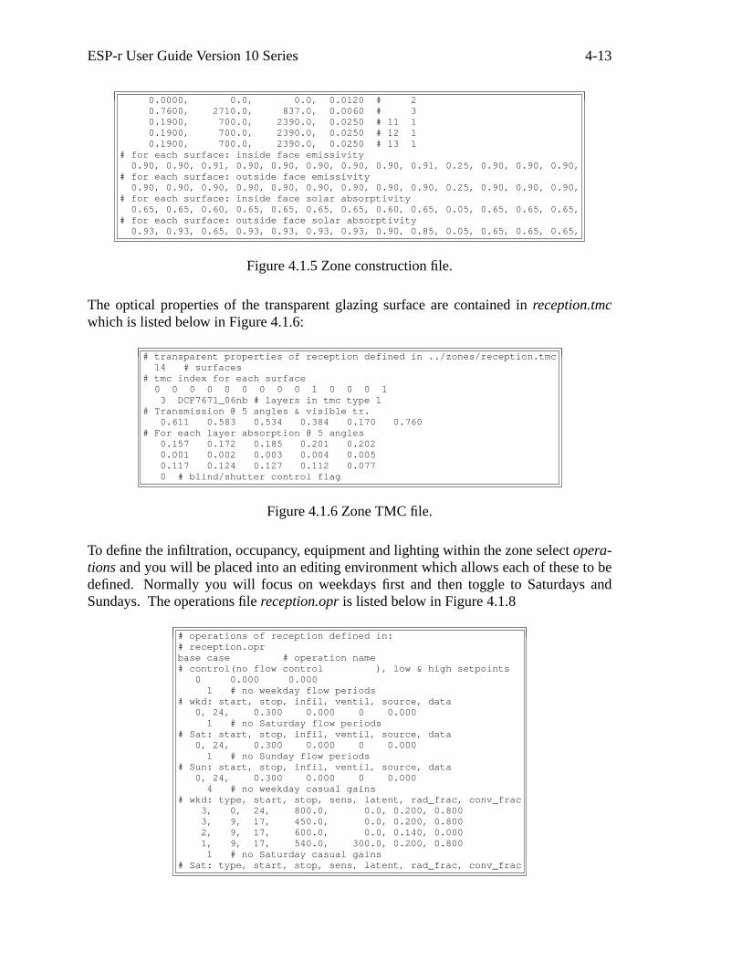
surface attributes) ESP-r will attempt to create the necessary files. During the creationprocess it will ask you to confirm that glz_s is transparent, otherwise the process is auto-matic. You may browse through any of the surfaces thermophysical properties and unlessa change is demanded the data can be merged into the problem. The thermophysicalproperties are contained in reception.con which is listed below in Figure 4.1.5.
# thermophysical properties of reception defined in reception.con# no of |air |surface(from geo)| multilayer construction# layers|gaps| no. name | database name
4, 1 # 1 south extern_wall4, 1 # 2 east extern_wall2, 0 # 3 passage intern_wall4, 1 # 4 north extern_wall4, 1 # 5 part_a extern_wall4, 1 # 6 part_b extern_wall4, 1 # 7 west extern_wall4, 1 # 8 ceiling roof_14, 0 # 9 floor floor_13, 1 # 10 glz_s d_glz1, 0 # 11 door_p door1, 0 # 12 door_a door1, 0 # 13 door_w door
3, 0.170, # air gap position & resistance for surface 13, 0.170, # air gap position & resistance for surface 23, 0.170, # air gap position & resistance for surface 43, 0.170, # air gap position & resistance for surface 53, 0.170,3, 0.170, # air gap position & resistance for surface 63, 0.170, # air gap position & resistance for surface 73, 0.170, # air gap position & resistance for surface 82, 0.170, # air gap position & resistance for surface 10
# conduc- | density | specific | thick- | surf|layer# tivity | | heat | ness(m)| |
0.9600, 2000.0, 650.0, 0.1000 # 1 10.0400, 250.0, 840.0, 0.0750 # 20.0000, 0.0, 0.0, 0.0500 # 30.4400, 1500.0, 650.0, 0.1000 # 40.9600, 2000.0, 650.0, 0.1000 # 2 10.0400, 250.0, 840.0, 0.0750 # 20.0000, 0.0, 0.0, 0.0500 # 30.4400, 1500.0, 650.0, 0.1000 # 40.4400, 1500.0, 650.0, 0.1500 # 3 10.1800, 800.0, 837.0, 0.0120 # 20.9600, 2000.0, 650.0, 0.1000 # 4 10.0400, 250.0, 840.0, 0.0750 # 20.0000, 0.0, 0.0, 0.0500 # 30.4400, 1500.0, 650.0, 0.1000 # 40.9600, 2000.0, 650.0, 0.1000 # 5 10.0400, 250.0, 840.0, 0.0750 # 20.0000, 0.0, 0.0, 0.0500 # 30.4400, 1500.0, 650.0, 0.1000 # 40.9600, 2000.0, 650.0, 0.1000 # 6 10.0400, 250.0, 840.0, 0.0750 # 20.0000, 0.0, 0.0, 0.0500 # 30.4400, 1500.0, 650.0, 0.1000 # 40.9600, 2000.0, 650.0, 0.1000 # 7 10.0400, 250.0, 840.0, 0.0750 # 20.0000, 0.0, 0.0, 0.0500 # 30.4400, 1500.0, 650.0, 0.1000 # 40.1900, 960.0, 837.0, 0.0120 # 8 10.3800, 1200.0, 653.0, 0.0500 # 20.0000, 0.0, 0.0, 0.0500 # 30.3800, 1120.0, 840.0, 0.0080 # 41.2800, 1460.0, 879.0, 0.1000 # 9 12.9000, 2650.0, 900.0, 0.1000 # 21.4000, 2100.0, 653.0, 0.0500 # 31.4000, 2100.0, 650.0, 0.0500 # 40.7600, 2710.0, 837.0, 0.0060 # 10 1
ESP-r User Guide Version 10 Series 4-13
0.0000, 0.0, 0.0, 0.0120 # 20.7600, 2710.0, 837.0, 0.0060 # 30.1900, 700.0, 2390.0, 0.0250 # 11 10.1900, 700.0, 2390.0, 0.0250 # 12 10.1900, 700.0, 2390.0, 0.0250 # 13 1
# for each surface: inside face emissivity0.90, 0.90, 0.91, 0.90, 0.90, 0.90, 0.90, 0.90, 0.91, 0.25, 0.90, 0.90, 0.90,
# for each surface: outside face emissivity0.90, 0.90, 0.90, 0.90, 0.90, 0.90, 0.90, 0.90, 0.90, 0.25, 0.90, 0.90, 0.90,
# for each surface: inside face solar absorptivity0.65, 0.65, 0.60, 0.65, 0.65, 0.65, 0.65, 0.60, 0.65, 0.05, 0.65, 0.65, 0.65,
# for each surface: outside face solar absorptivity0.93, 0.93, 0.65, 0.93, 0.93, 0.93, 0.93, 0.90, 0.85, 0.05, 0.65, 0.65, 0.65,
Figure 4.1.5 Zone construction file.
The optical properties of the transparent glazing surface are contained in reception.tmcwhich is listed below in Figure 4.1.6:
# transparent properties of reception defined in ../zones/reception.tmc14 # surfaces
# tmc index for each surface0 0 0 0 0 0 0 0 0 1 0 0 0 13 DCF7671_06nb # layers in tmc type 1
# Transmission @ 5 angles & visible tr.0.611 0.583 0.534 0.384 0.170 0.760
# For each layer absorption @ 5 angles0.157 0.172 0.185 0.201 0.2020.001 0.002 0.003 0.004 0.0050.117 0.124 0.127 0.112 0.0770 # blind/shutter control flag
Figure 4.1.6 Zone TMC file.
To define the infiltration, occupancy, equipment and lighting within the zone select opera-tions and you will be placed into an editing environment which allows each of these to bedefined. Normally you will focus on weekdays first and then toggle to Saturdays andSundays. The operations file reception.opr is listed below in Figure 4.1.8
# operations of reception defined in:# reception.oprbase case # operation name# control(no flow control ), low & high setpoints
0 0.000 0.0001 # no weekday flow periods
# wkd: start, stop, infil, ventil, source, data0, 24, 0.300 0.000 0 0.000
1 # no Saturday flow periods# Sat: start, stop, infil, ventil, source, data
0, 24, 0.300 0.000 0 0.0001 # no Sunday flow periods
# Sun: start, stop, infil, ventil, source, data0, 24, 0.300 0.000 0 0.000
4 # no weekday casual gains# wkd: type, start, stop, sens, latent, rad_frac, conv_frac
3, 0, 24, 800.0, 0.0, 0.200, 0.8003, 9, 17, 450.0, 0.0, 0.200, 0.8002, 9, 17, 600.0, 0.0, 0.140, 0.0001, 9, 17, 540.0, 300.0, 0.200, 0.8001 # no Saturday casual gains
# Sat: type, start, stop, sens, latent, rad_frac, conv_frac

ESP-r User Guide Version 10 Series 4-14
3, 0, 24, 800.0, 0.0, 0.200, 0.8001 # no Sunday casual gains
# Sun: type, start, stop, sens, latent, rad_frac, conv_frac3, 0, 24, 800.0, 0.0, 0.200, 0.800
Figure 4.1.8 Zone operation file.
There are several points within ESP-r where information related to the problem topologycan be supplied. Within the problem definition menu there is the connection and bound-ary selection which allows one or more of the connections to be manually edited, topol-ogy to be checked and generated via a vertex matching algorithm or topology to beimported from surface attribute boundary specifications. Within the geometry browse &edit facility you may specify boundary conditions as surface attributes or import the con-nection topology to the surface attributes.
By definition, the initial assumption for the topology of a problem is that all surfaces facethe outside. This can be confirmed by exiting to the problem definition menu and consult-ing the connection and boundary selection. As most of the walls face the outside a quickway to update the surface boundary attributes is to return to the geometry browse & editand select update topology from problem.
Tw o surfaces in the zone do not face the outside and this can be defined in two ways:
1) supply the boundary for the other side of the ’passage’ and the ’floor’ as surfaceattributes and then exit to the connection and boundary and import this informationor;
2) edit the connection in the connection and boundary display and then move to thegeometry browse & edit and import the information.
After updating the problem (system configuration) file simple_office should look like thelisting in Figure 4.1.9
* CONFIGURATION3.0# ESRU system configuration defined by file# bld_basic.cfg*date Mon Jun 26 16:50:29 2000 # latest file modification*root bld_basic*zonpth ../zones # path to zones*netpth ../networks # path to networks*ctlpth ../ctl # path to controls*radpth ../rad # path to radiance files*imgpth ../images # path to project images*indx 1 # Building only51.700 -0.500 # Latitude & Longitude (diff from meridian)
2 0.200 # Site exposure & ground reflectivity* DATABASES*prm /usr/esru/esp-r/databases/constr.db2*mlc /usr/esru/esp-r/databases/multicon.db2*opt /usr/esru/esp-r/databases/optics.db2*prs /usr/esru/esp-r/databases/pressc.db1*evn /usr/esru/esp-r/databases/profiles.db1*clm /usr/esru/esp-r/climate/clm67*pdb /usr/esru/esp-r/databases/plantc.db1*ctl ../ctl/bld_basic.ctl*year 1967 # assessment year*img GIF FZON ../images/basic_montg.gif*img GIF FZON ../images/foyer.gif*img GIF **** ../images/daylight.gif

ESP-r User Guide Version 10 Series 4-15
# prim energy conv (heat,cool,lights,fan,sml pwr,hot water)*pecnv 1.250 3.600 3.600 3.600 3.600 1.250*htemis 190.000 0.200 0.100 # heating emissions CO2,NOX,SOX*clemis 612.000 2.060 7.500 # cooling emissions CO2,NOX,SOX*ltemis 612.000 2.060 7.500 # lighting emissions CO2,NOX,SOX*fnemis 612.000 2.060 7.500 # fan/pump emissions CO2,NOX,SOX*spemis 612.000 2.060 7.500 # small power emissions CO2,NOX,SOX*hwemis 190.000 0.200 0.100 # dhw emissions CO2,NOX,SOX*ipv bld_basic.ipv# sim setup: no. sets startup zone_ts plant_ts save_lv*sps 4 3 1 10 2
9 1 15 1 def # period & name*sblr bld_basic_def.res*sipv*end_set
9 1 15 1 win # period & name*sblr bld_basic_win.res*sipv bld_basicwin_ipv.rep*end_set
6 3 12 3 trn # period & name*sblr bld_basic_trn.res*sipv bld_basictrn_ipv.rep*end_set
11 7 17 7 sum # period & name*sblr bld_basic_sum.res*sipv bld_basicsum_ipv.rep*end_set*end_sps* PROJ LOGbld_basic.log* Ground*mgp 1
4.60 2.80 3.30 5.10 6.10 9.60 11.40 13.60 14.30 12.70 7.50 5.50*end* BuildingBasic 3 zone model.
3 # no of zones*zon 1 # reference for reception*opr ../zones/reception.opr # schedules*geo ../zones/reception.geo # geometry*con ../zones/reception.con # construction*tmc ../zones/reception.tmc # transparent constr*zend*zon 2 # reference for office*opr ../zones/office.opr # schedules*geo ../zones/office.geo # geometry*con ../zones/office.con # construction*tmc ../zones/office.tmc # transparent constr*zend*zon 3 # reference for roof_space*opr ../zones/roof_space.opr # schedules*geo ../zones/roof_space.geo # geometry*con ../zones/roof_space.con # construction*zend*cnn bld_basic.cnn # connections
0 # no fluid flow network
Figure 4.1.9 Problem definition (system configuration) file.
Now a configuration control file must be created using the building controls & actuationfacility. This file contains the control statements to be obeyed by the Simulator at simula-tion time. This file can be confusing for some users of ESP-r. Previous releases providedonly minimal editing facilities, however ESP-r includes a extensive editing and reportingfacilities which should ease the process considerably.
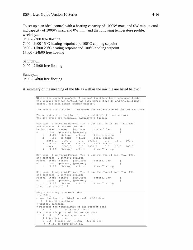
ESP-r User Guide Version 10 Series 4-16
To set up a an ideal control with a heating capacity of 1000W max. and 0W min., a cool-ing capacity of 1000W max. and 0W min. and the following temperature profile:weekday....0h00 - 7h00 free floating7h00 - 9h00 15°C heating setpoint and 100°C cooling setpoint9h00 - 17h00 20°C heating setpoint and 100°C cooling setpoint17h00 - 24h00 free floating
Saturday....0h00 - 24h00 free floating
Sunday....0h00 - 24h00 free floating
A summary of the meaning of the file as well as the raw file are listed below:
Within the current project 1 control functions have been specified.The overall project control has been named <test 1> and the buildingcontrol has been named <summer/winter>.
The sensor for function 1 measures the temperature of the current zone.
The actuator for function 1 is air point of the current zoneThe day types are Weekdays, Saturdays & Sundays
Day type 1 is valid Period: Tue 1 Jan To: Tue 31 Dec YEAR:1991and contains 4 control periods.Period| Start |sensed |actuated | control law |no | time |property |property | |
1 0.00 db temp > flux free floating2 7.00 db temp > flux ideal control
data... 1000.0 0.0 1000.0 0.0 15.0 100.03 9.00 db temp > flux ideal control
data... 1000.0 0.0 1000.0 0.0 20.0 100.04 18.00 db temp > flux free floating
Day type 2 is valid Period: Tue 1 Jan To: Tue 31 Dec YEAR:1991and contains 1 control periods.Period| Start |sensed |actuated | control law |no | time |property |property | |
1 0.00 db temp > flux free floating
Day type 3 is valid Period: Tue 1 Jan To: Tue 31 Dec YEAR:1991and contains 1 control periods.Period| Start |sensed |actuated | control law |no | time |property |property | |
1 0.00 db temp > flux free floatingzone 1 << control 1
simple building # overall descr* Buildingconvective heating, ideal control # bld descr
1 # No. of functions* Control function# measures the temperature of the current zone.
0 0 0 0 # sensor data# actuates air point of the current zone
0 0 0 # actuator data0 # No. day types1 365 # valid Sun 1 Jan - Sun 31 Dec4 # No. of periods in day

ESP-r User Guide Version 10 Series 4-17
0 2 0.000 # ctl type, law (free floating), start @0. # No. of data items
0 1 7.000 # ctl type, law (ideal control), start @6. # No. of data items
1000.000 0.000 0.000 0.000 20.000 100.0000 1 9.000 # ctl type, law (ideal control), start @6. # No. of data items
1000.000 0.000 0.000 0.000 20.000 100.0000 2 18.000 # ctl type, law (free floating), start @0. # No. of data items
1 365 # valid Sun 1 Jan - Sun 31 Dec1 # No. of periods in day
0 2 0.000 # ctl type, law (free floating), start @0. # No. of data items
1 365 # valid Sun 1 Jan - Sun 31 Dec1 # No. of periods in day
0 2 0.000 # ctl type, law (free floating), start @0. # No. of data items
# Function:Zone links1 1 0
Figure 4.1.10 System control information and file.
A simulation is now performed via the Simulator using the climate file ˜esru/esp-r/cli-mate/clm67. Two simulations should be performed, saving both in the same results librarycalled, for example, ex1.res. The first should span the period 9th January to 15 Januaryinclusive. The second should span the period 11 July to 17 July inclusive. Both simula-tions should have a one hour time-step.
Now Results Analysis Module is used to see the results obtained from the simulation.After entering the library name (ex1.res in this case) you can select graph, time-variableand inside air temperature to obtain a common temperature-profile of the inside air.According to these profiles (see figures), the following items can be discussed (youshould generate these profiles yourself):
1) In winter the maximum heating capacity of the actuated control is not satisfactoryto achieve the heating setpoint (20°C from 9h00 to 18h00) of the inside air. To per-form the next simulation, you can change this maximum heating capacity forinstance up to 3000 [W], you will notice that now -during weekdays- the setpointtemperature is reached during the afternoon (figure 4.1.11 and 4.1.13). The newcontrol file is listed below in figure 4.1.12.
2) In summer the cooling setpoint (100°C from 7h00 to 18h00) never actuates thecooling capacity because this setpoint-temperature never occurs. In the new controlfile (figure 4.1.11) this setpoint-temperature is adapted to 25°C actuating a coolingcapacity of 3000 W. If you generate a temperature-profile now you can see that theinside air temperature is decreased during weekday.
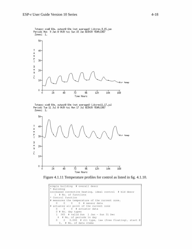
ESP-r User Guide Version 10 Series 4-18
Figure 4.1.11 Temperature profiles for control as listed in fig. 4.1.10.
simple building # overall descr* Buildingincreased convective heating, ideal control # bld descr
1 # No. of functions* Control function# measures the temperature of the current zone.
0 0 0 0 # sensor data# actuates air point of the current zone
0 0 0 # actuator data0 # No. day types1 365 # valid Sun 1 Jan - Sun 31 Dec4 # No. of periods in day
0 2 0.000 # ctl type, law (free floating), start @0. # No. of data items
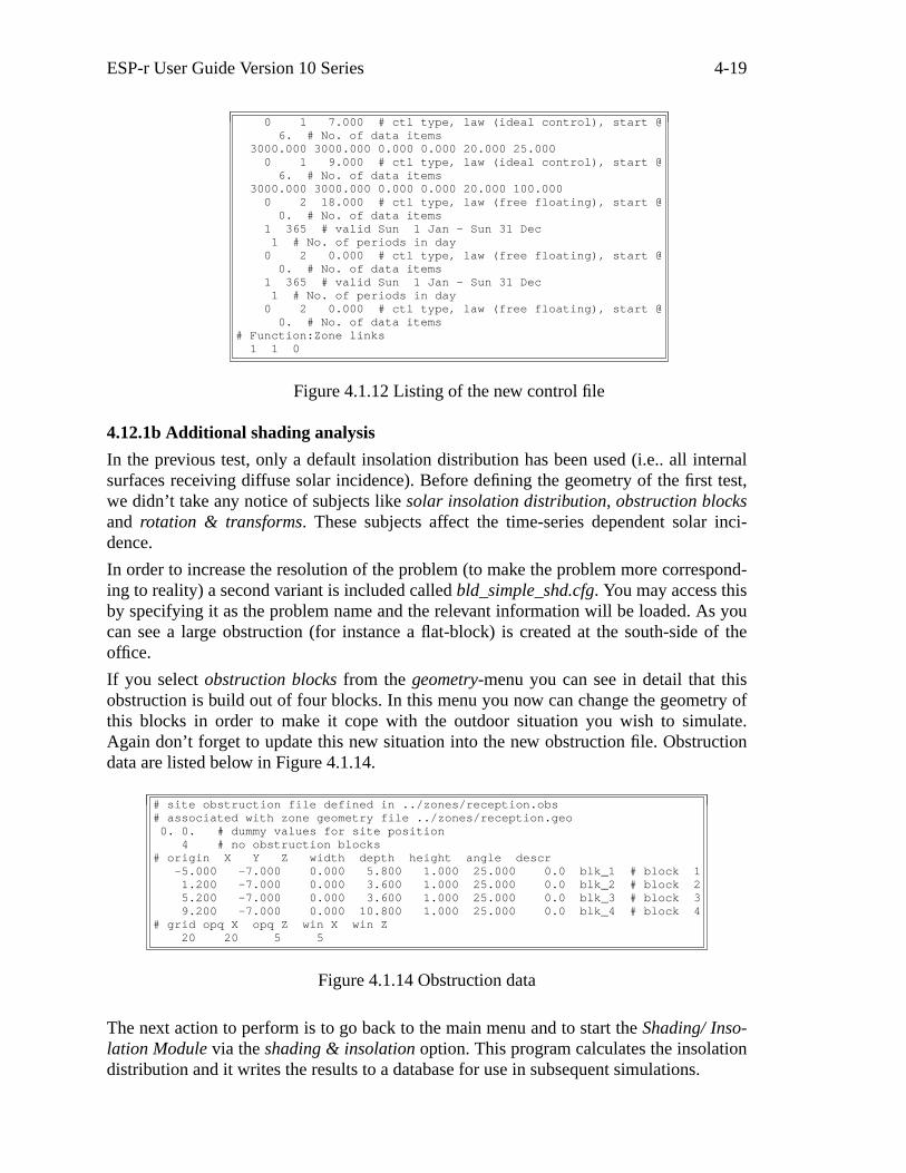
ESP-r User Guide Version 10 Series 4-19
0 1 7.000 # ctl type, law (ideal control), start @6. # No. of data items
3000.000 3000.000 0.000 0.000 20.000 25.0000 1 9.000 # ctl type, law (ideal control), start @6. # No. of data items
3000.000 3000.000 0.000 0.000 20.000 100.0000 2 18.000 # ctl type, law (free floating), start @0. # No. of data items
1 365 # valid Sun 1 Jan - Sun 31 Dec1 # No. of periods in day
0 2 0.000 # ctl type, law (free floating), start @0. # No. of data items
1 365 # valid Sun 1 Jan - Sun 31 Dec1 # No. of periods in day
0 2 0.000 # ctl type, law (free floating), start @0. # No. of data items
# Function:Zone links1 1 0
Figure 4.1.12 Listing of the new control file
4.12.1b Additional shading analysis
In the previous test, only a default insolation distribution has been used (i.e.. all internalsurfaces receiving diffuse solar incidence). Before defining the geometry of the first test,we didn’t take any notice of subjects like solar insolation distribution, obstruction blocksand rotation & transforms. These subjects affect the time-series dependent solar inci-dence.
In order to increase the resolution of the problem (to make the problem more correspond-ing to reality) a second variant is included called bld_simple_shd.cfg. You may access thisby specifying it as the problem name and the relevant information will be loaded. As youcan see a large obstruction (for instance a flat-block) is created at the south-side of theoffice.
If you select obstruction blocks from the geometry-menu you can see in detail that thisobstruction is build out of four blocks. In this menu you now can change the geometry ofthis blocks in order to make it cope with the outdoor situation you wish to simulate.Again don’t forget to update this new situation into the new obstruction file. Obstructiondata are listed below in Figure 4.1.14.
# site obstruction file defined in ../zones/reception.obs# associated with zone geometry file ../zones/reception.geo0. 0. # dummy values for site position
4 # no obstruction blocks# origin X Y Z width depth height angle descr
-5.000 -7.000 0.000 5.800 1.000 25.000 0.0 blk_1 # block 11.200 -7.000 0.000 3.600 1.000 25.000 0.0 blk_2 # block 25.200 -7.000 0.000 3.600 1.000 25.000 0.0 blk_3 # block 39.200 -7.000 0.000 10.800 1.000 25.000 0.0 blk_4 # block 4
# grid opq X opq Z win X win Z20 20 5 5
Figure 4.1.14 Obstruction data
The next action to perform is to go back to the main menu and to start the Shading/ Inso-lation Module via the shading & insolation option. This program calculates the insolationdistribution and it writes the results to a database for use in subsequent simulations.

ESP-r User Guide Version 10 Series 4-20
Figure 4.1.13 Temperature profiles for control as listed in fig. 4.1.12.
The results that you will obtain now show no difference in winter. In this period the solarradiation is not remarkable. However in summer (cooling capacity 1000 W, actuated at25°C) a slight difference occurs as you can see from Figure 4.1.15. Note that in these fig-ures the internal and external surface temperatures of the south wall are drawn instead ofthe inside air temperature.
If no shading/insolation database exists, the default insolation distribution of the zoneoperations file will be used. In this case ESP-r assumes no obstructions so that only thebuilding geometry is needed for calculation of the insolation distribution.
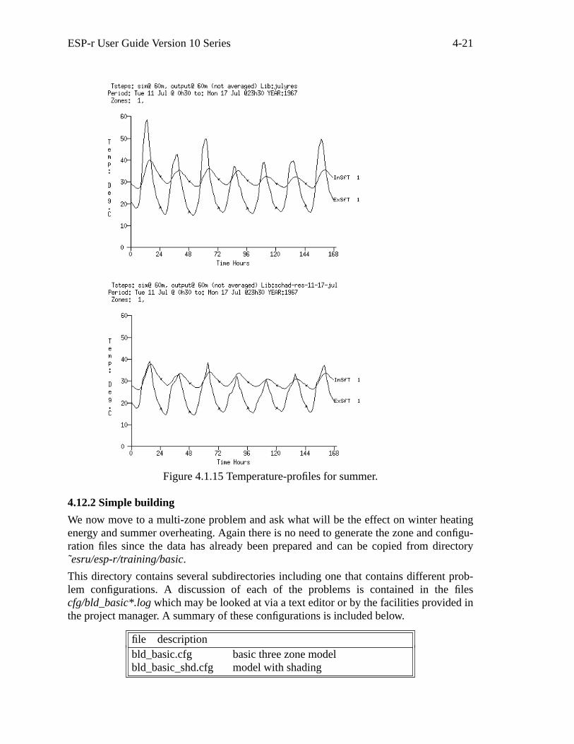
ESP-r User Guide Version 10 Series 4-21
Figure 4.1.15 Temperature-profiles for summer.
4.12.2 Simple building
We now move to a multi-zone problem and ask what will be the effect on winter heatingenergy and summer overheating. Again there is no need to generate the zone and configu-ration files since the data has already been prepared and can be copied from directory˜esru/esp-r/training/basic.
This directory contains several subdirectories including one that contains different prob-lem configurations. A discussion of each of the problems is contained in the filescfg/bld_basic*.log which may be looked at via a text editor or by the facilities provided inthe project manager. A summary of these configurations is included below.
file descriptionbld_basic.cfg basic three zone modelbld_basic_shd.cfg model with shading
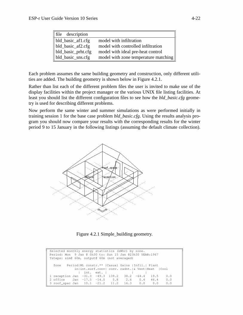
ESP-r User Guide Version 10 Series 4-22
file descriptionbld_basic_af1.cfg model with infiltrationbld_basic_af2.cfg model with controlled infiltrationbld_basic_prht.cfg model with ideal pre-heat controlbld_basic_sns.cfg model with zone temperature matching
Each problem assumes the same building geometry and construction, only different utili-ties are added. The building geometry is shown below in Figure 4.2.1.
Rather than list each of the different problem files the user is invited to make use of thedisplay facilities within the project manager or the various UNIX file listing facilities. Atleast you should list the different configuration files to see how the bld_basic.cfg geome-try is used for describing different problems.
Now perform the same winter and summer simulations as were performed initially intraining session 1 for the base case problem bld_basic.cfg. Using the results analysis pro-gram you should now compare your results with the corresponding results for the winterperiod 9 to 15 January in the following listings (assuming the default climate collection).
Figure 4.2.1 Simple_building geometry.
Selected monthly energy statistics (kWhr) by zone.Period: Mon 9 Jan @ 0h30 to: Sun 15 Jan @23h30 YEAR:1967Tsteps: sim@ 60m, output@ 60m (not averaged)
Zone Period|ML constr.** |Casual Gains |Infil.| Plantin|int.surf.conv| conv. radnt.|& Vent|Heat |Cool| int. ext. | | |
1 reception Jan -31.3 -49.3 139.2 38.2 -64.4 19.5 0.02 office Jan -17.5 -14.0 5.8 2.6 0.4 46.4 0.03 roof_spac Jan 10.1 -21.2 11.2 16.3 0.0 0.0 0.0

ESP-r User Guide Version 10 Series 4-23
All zones Jan -39. -85. 156. 57. -64. 66. 0.
** Opaque & transparent multilayer construction: viaconduction from surfaces facing zone (internal/external).
Note that connections to ground are considered internal.
Interrogation output for result-set 1Period: Mon 9 Jan @ 0h30 to: Sun 15 Jan @23h30 YEAR:1967Tsteps: sim@ 60m, output@ 60m (not averaged)
Zone radiant & convective plant used (kWhrs)Zone Heating Cooling
id name Energy No. of Energy No. of(kWhrs) Hr rqd (kWhrs) Hr rqd
1 reception 19.541 39.0 0.000 0.02 office 46.428 60.0 0.000 0.03 roof_space 0.000 0.0 0.000 0.0
All 65.969 0.000
Casual gains summary (kWhrs) for zone 1: receptionPeriod: Mon 9 Jan @ 0h30 to: Sun 15 Jan @23h30 YEAR:1967Tsteps: sim@ 60m, output@ 60m (not averaged)
Casual gain | Convect | Total | Radiant by connection type| portion | Radiant | external internal ground
UC type 1 @opq 17.280 4.271 1.133 3.139 0.000UC type 1 @trn 0.049 0.049 0.000 0.000UC type 2 @opq 0.000 3.322 0.881 2.441 0.000UC type 2 @trn 0.038 0.038 0.000 0.000UC type 3 @opq 121.920 30.137 7.992 22.145 0.000UC type 3 @trn 0.343 0.343 0.000 0.000Totals 139.200 38.160 10.435 27.725 0.000
@opq = associated with opaque MLC,@trn = associated with transparent MLC,UC = uncontrolled, C = controlled, all in kWhr.
Causal energy breakdown (kWhrs) at air point for zone 1: receptionPeriod: Mon 9 Jan @ 0h30 to: Sun 15 Jan @23h30 YEAR:1967Tsteps: sim@ 60m, output@ 60m (not averaged)
Gain LossInfiltration air load 0.000 -35.797Ventilation air load 0.179 -28.828Uncontr‘d casual type 1 17.280 0.000Uncontr‘d casual type 2 0.000 0.000Uncontr‘d casual type 3 121.920 0.000Opaque MLC convec: ext 0.000 -28.412Opaque MLC convec: int 2.765 -34.043Transp MLC convec: ext 0.021 -20.900Transp MLC convec: int 0.000 0.000Convec portion of plant 19.541 0.000Totals 162.215 -162.104
Causal energy breakdown (Whrs) for south ( 1) in reception ( 1)Surface is opaque MLC, area= 16.50m2 & connects to the outsidePeriod: Mon 9 Jan @ 0h30 to: Sun 15 Jan @23h30 YEAR:1967Tsteps: sim@ 60m, output@ 60m (not averaged)
Facing Zone 1 Facing Zone 0Gain Loss Gain Loss
Conductive flux 0.00 -16106.23 29184.56 -15845.35Convective flux 7822.55 -6.54 10173.91 -13390.11Longwave rad int 4049.18 -325.08 -- --LW rad ext >bldg -- -- 20.32 -1908.40LW rad ext >sky -- -- 0.00 -64480.62LW rad ext >grnd -- -- 11175.86 -1975.07Shortwave rad. 1408.22 0.00 47656.58 0.00Unctrl cas typ 1 385.34 0.00 -- --
cas typ 2 299.71 0.00 -- --cas typ 3 2718.81 0.00 -- --
Heat stored 1837.48 -2083.43 8037.96 -8649.63

ESP-r User Guide Version 10 Series 4-24
Plant 0.00 0.00 0.00 0.00Totals 18521.29 -18521.28 106249.20 -106249.19
Casual gains summary (kWhrs) for zone 2: officePeriod: Mon 9 Jan @ 0h30 to: Sun 15 Jan @23h30 YEAR:1967Tsteps: sim@ 60m, output@ 60m (not averaged)
Casual gain | Convect | Total | Radiant by connection type| portion | Radiant | external internal ground
UC type 1 @opq 5.760 1.440 0.397 0.744 0.299UC type 1 @trn 0.000 0.000 0.000 0.000UC type 2 @opq 0.000 1.120 0.309 0.578 0.233UC type 2 @trn 0.000 0.000 0.000 0.000UC type 3 @opq 0.000 0.000 0.000 0.000 0.000UC type 3 @trn 0.000 0.000 0.000 0.000Totals 5.760 2.560 0.706 1.322 0.532
@opq = associated with opaque MLC,@trn = associated with transparent MLC,UC = uncontrolled, C = controlled, all in kWhr.
Causal energy breakdown (kWhrs) at air point for zone 2: officePeriod: Mon 9 Jan @ 0h30 to: Sun 15 Jan @23h30 YEAR:1967Tsteps: sim@ 60m, output@ 60m (not averaged)
Gain LossInfiltration air load 0.000 -9.078Ventilation air load 9.531 -0.017Uncontr‘d casual type 1 5.760 0.000Uncontr‘d casual type 2 0.000 0.000Uncontr‘d casual type 3 0.000 0.000Opaque MLC convec: ext 1.244 -15.231Opaque MLC convec: int 4.804 -22.338Transp MLC convec: ext 0.000 0.000Transp MLC convec: int 0.000 0.000Convec portion of plant 46.428 0.000Totals 67.987 -67.952
Figure 4.2.2 Tabular statistics during winter simulation period.
From this tabular report you can see that during the simulation period, the office requiresmost heating energy (46 kWh) while the reception looses most energy (160 kWh). Theenergy statistics table and the causal energy breakdown table show that the reception zoneloses most energy due to conduction (total 80 kWh). However the reception zone alsosuffers a high casual gain from equipment (type 3) so the reception net heat loss is lessthan the office net heat loss.
If you look to the operation files you will see that a coupled air flow from the receptioninto the office is defined. In the listed energy statistics you can see that (due to this inter-zonal airflow) the heat loss from the reception to the office is more or less 10 kWh.
Next you should perform the same simulation for the summer (11-17 July) and generate atabular report. You will obtain results as listed below.
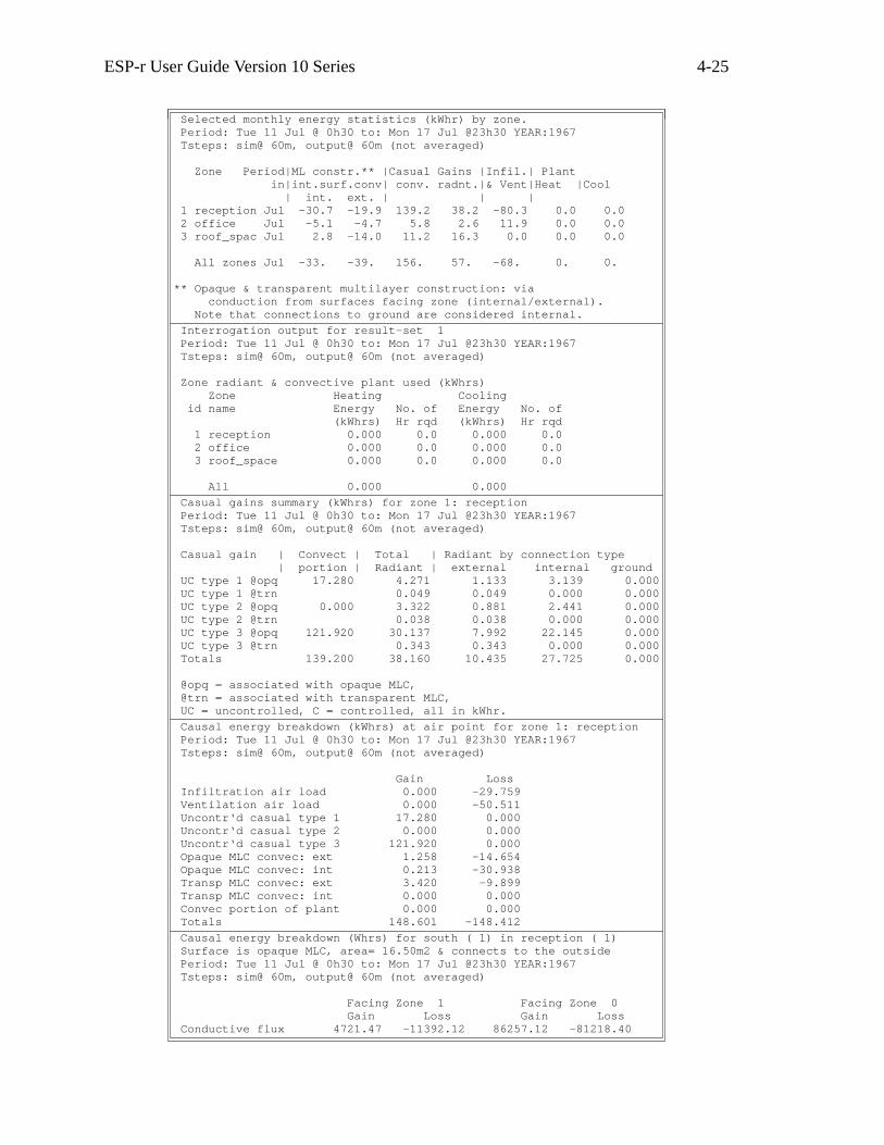
ESP-r User Guide Version 10 Series 4-25
Selected monthly energy statistics (kWhr) by zone.Period: Tue 11 Jul @ 0h30 to: Mon 17 Jul @23h30 YEAR:1967Tsteps: sim@ 60m, output@ 60m (not averaged)
Zone Period|ML constr.** |Casual Gains |Infil.| Plantin|int.surf.conv| conv. radnt.|& Vent|Heat |Cool| int. ext. | | |
1 reception Jul -30.7 -19.9 139.2 38.2 -80.3 0.0 0.02 office Jul -5.1 -4.7 5.8 2.6 11.9 0.0 0.03 roof_spac Jul 2.8 -14.0 11.2 16.3 0.0 0.0 0.0
All zones Jul -33. -39. 156. 57. -68. 0. 0.
** Opaque & transparent multilayer construction: viaconduction from surfaces facing zone (internal/external).
Note that connections to ground are considered internal.
Interrogation output for result-set 1Period: Tue 11 Jul @ 0h30 to: Mon 17 Jul @23h30 YEAR:1967Tsteps: sim@ 60m, output@ 60m (not averaged)
Zone radiant & convective plant used (kWhrs)Zone Heating Cooling
id name Energy No. of Energy No. of(kWhrs) Hr rqd (kWhrs) Hr rqd
1 reception 0.000 0.0 0.000 0.02 office 0.000 0.0 0.000 0.03 roof_space 0.000 0.0 0.000 0.0
All 0.000 0.000
Casual gains summary (kWhrs) for zone 1: receptionPeriod: Tue 11 Jul @ 0h30 to: Mon 17 Jul @23h30 YEAR:1967Tsteps: sim@ 60m, output@ 60m (not averaged)
Casual gain | Convect | Total | Radiant by connection type| portion | Radiant | external internal ground
UC type 1 @opq 17.280 4.271 1.133 3.139 0.000UC type 1 @trn 0.049 0.049 0.000 0.000UC type 2 @opq 0.000 3.322 0.881 2.441 0.000UC type 2 @trn 0.038 0.038 0.000 0.000UC type 3 @opq 121.920 30.137 7.992 22.145 0.000UC type 3 @trn 0.343 0.343 0.000 0.000Totals 139.200 38.160 10.435 27.725 0.000
@opq = associated with opaque MLC,@trn = associated with transparent MLC,UC = uncontrolled, C = controlled, all in kWhr.
Causal energy breakdown (kWhrs) at air point for zone 1: receptionPeriod: Tue 11 Jul @ 0h30 to: Mon 17 Jul @23h30 YEAR:1967Tsteps: sim@ 60m, output@ 60m (not averaged)
Gain LossInfiltration air load 0.000 -29.759Ventilation air load 0.000 -50.511Uncontr‘d casual type 1 17.280 0.000Uncontr‘d casual type 2 0.000 0.000Uncontr‘d casual type 3 121.920 0.000Opaque MLC convec: ext 1.258 -14.654Opaque MLC convec: int 0.213 -30.938Transp MLC convec: ext 3.420 -9.899Transp MLC convec: int 0.000 0.000Convec portion of plant 0.000 0.000Totals 148.601 -148.412
Causal energy breakdown (Whrs) for south ( 1) in reception ( 1)Surface is opaque MLC, area= 16.50m2 & connects to the outsidePeriod: Tue 11 Jul @ 0h30 to: Mon 17 Jul @23h30 YEAR:1967Tsteps: sim@ 60m, output@ 60m (not averaged)
Facing Zone 1 Facing Zone 0Gain Loss Gain Loss
Conductive flux 4721.47 -11392.12 86257.12 -81218.40
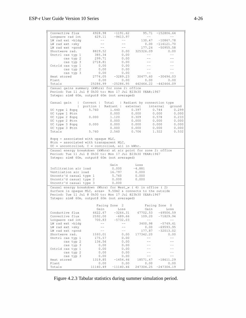
ESP-r User Guide Version 10 Series 4-26
Convective flux 4928.98 -1191.62 95.71 -152806.64Longwave rad int 629.11 -9413.97 -- --LW rad ext >bldg -- -- 130.47 -10867.78LW rad ext >sky -- -- 0.00 -116121.70LW rad ext >grnd -- -- 177.24 -50955.58Shortwave rad. 8829.52 0.00 325326.09 0.00Unctrl cas typ 1 385.34 0.00 -- --
cas typ 2 299.71 0.00 -- --cas typ 3 2718.81 0.00 -- --
Cntrld cas typ 1 0.00 0.00 -- --cas typ 2 0.00 0.00 -- --cas typ 3 0.00 0.00 -- --
Heat stored 2774.05 -3289.23 30477.60 -30494.03Plant 0.00 0.00 0.00 0.00Totals 25286.99 -25286.95 442464.22 -442464.09
Casual gains summary (kWhrs) for zone 2: officePeriod: Tue 11 Jul @ 0h30 to: Mon 17 Jul @23h30 YEAR:1967Tsteps: sim@ 60m, output@ 60m (not averaged)
Casual gain | Convect | Total | Radiant by connection type| portion | Radiant | external internal ground
UC type 1 @opq 5.760 1.440 0.397 0.744 0.299UC type 1 @trn 0.000 0.000 0.000 0.000UC type 2 @opq 0.000 1.120 0.309 0.578 0.233UC type 2 @trn 0.000 0.000 0.000 0.000UC type 3 @opq 0.000 0.000 0.000 0.000 0.000UC type 3 @trn 0.000 0.000 0.000 0.000Totals 5.760 2.560 0.706 1.322 0.532
@opq = associated with opaque MLC,@trn = associated with transparent MLC,UC = uncontrolled, C = controlled, all in kWhr.
Causal energy breakdown (kWhrs) at air point for zone 2: officePeriod: Tue 11 Jul @ 0h30 to: Mon 17 Jul @23h30 YEAR:1967Tsteps: sim@ 60m, output@ 60m (not averaged)
Gain LossInfiltration air load 0.000 -4.881Ventilation air load 16.797 0.000Uncontr‘d casual type 1 5.760 0.000Uncontr‘d casual type 2 0.000 0.000Uncontr‘d casual type 3 0.000
Causal energy breakdown (Whrs) for West_w ( 4) in office ( 2)Surface is opaque MLC, area= 9.50m2 & connects to the outsidePeriod: Tue 11 Jul @ 0h30 to: Mon 17 Jul @23h30 YEAR:1967Tsteps: sim@ 60m, output@ 60m (not averaged)
Facing Zone 2 Facing Zone 0Gain Loss Gain Loss
Conductive flux 4622.67 -3264.31 47702.53 -49506.59Convective flux 2592.00 -689.66 109.20 -71829.94Longwave rad int 700.83 -5732.03 -- --LW rad ext >bldg -- -- 3400.98 -5749.41LW rad ext >sky -- -- 0.00 -69593.95LW rad ext >grnd -- -- 177.87 -32013.02Shortwave rad. 1593.01 0.00 177342.20 0.00Unctrl cas typ 1 175.57 0.00 -- --
cas typ 2 136.56 0.00 -- --cas typ 3 0.00 0.00 -- --
Cntrld cas typ 1 0.00 0.00 -- --cas typ 2 0.00 0.00 -- --cas typ 3 0.00 0.00 -- --
Heat stored 1319.85 -1454.46 18571.47 -18611.29Plant 0.00 0.00 0.00 0.00Totals 11140.49 -11140.46 247304.25 -247304.19
Figure 4.2.3 Tabular statistics during summer simulation period.
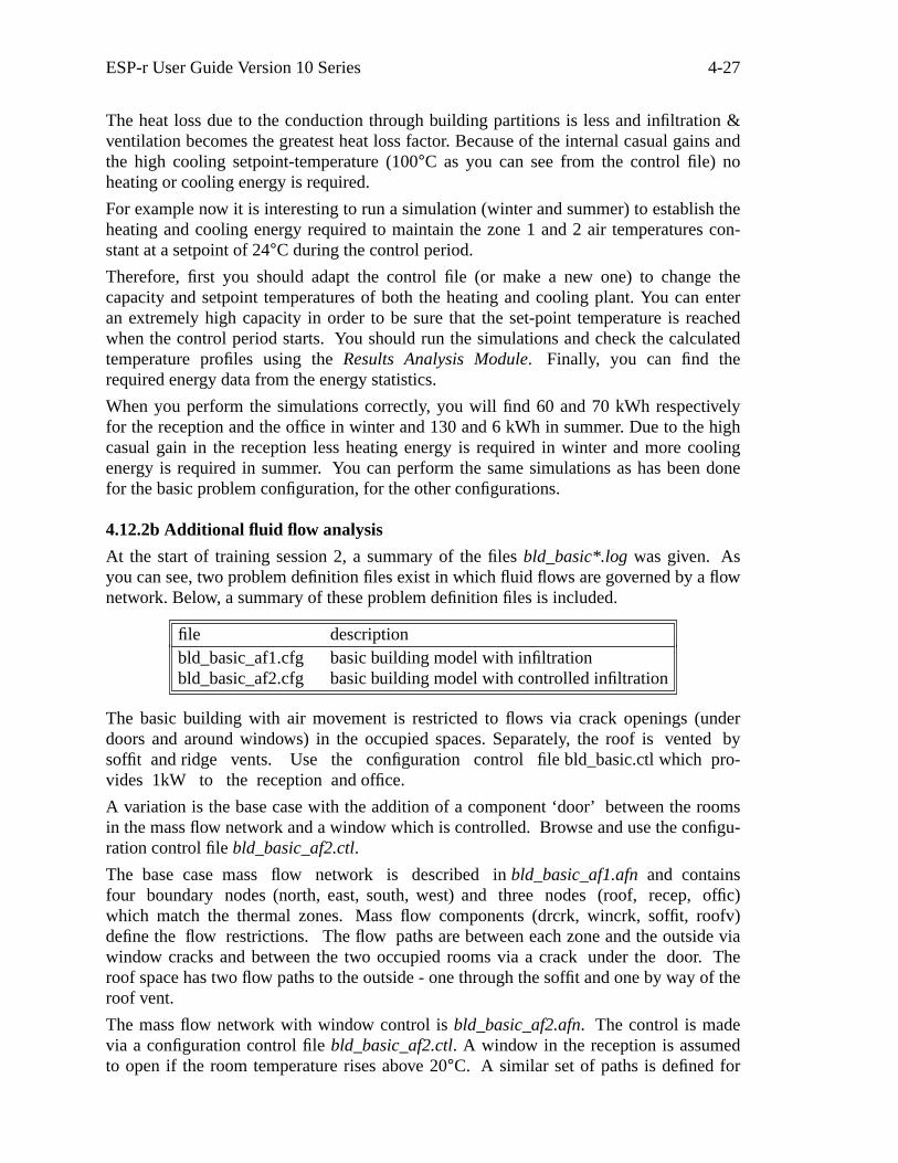
ESP-r User Guide Version 10 Series 4-27
The heat loss due to the conduction through building partitions is less and infiltration &ventilation becomes the greatest heat loss factor. Because of the internal casual gains andthe high cooling setpoint-temperature (100°C as you can see from the control file) noheating or cooling energy is required.
For example now it is interesting to run a simulation (winter and summer) to establish theheating and cooling energy required to maintain the zone 1 and 2 air temperatures con-stant at a setpoint of 24°C during the control period.
Therefore, first you should adapt the control file (or make a new one) to change thecapacity and setpoint temperatures of both the heating and cooling plant. You can enteran extremely high capacity in order to be sure that the set-point temperature is reachedwhen the control period starts. You should run the simulations and check the calculatedtemperature profiles using the Results Analysis Module. Finally, you can find therequired energy data from the energy statistics.
When you perform the simulations correctly, you will find 60 and 70 kWh respectivelyfor the reception and the office in winter and 130 and 6 kWh in summer. Due to the highcasual gain in the reception less heating energy is required in winter and more coolingenergy is required in summer. You can perform the same simulations as has been donefor the basic problem configuration, for the other configurations.
4.12.2b Additional fluid flow analysis
At the start of training session 2, a summary of the files bld_basic*.log was giv en. Asyou can see, two problem definition files exist in which fluid flows are governed by a flownetwork. Below, a summary of these problem definition files is included.
file descriptionbld_basic_af1.cfg basic building model with infiltrationbld_basic_af2.cfg basic building model with controlled infiltration
The basic building with air movement is restricted to flows via crack openings (underdoors and around windows) in the occupied spaces. Separately, the roof is vented bysoffit and ridge vents. Use the configuration control file bld_basic.ctl which pro-vides 1kW to the reception and office.
A variation is the base case with the addition of a component ‘door’ between the roomsin the mass flow network and a window which is controlled. Browse and use the configu-ration control file bld_basic_af2.ctl.
The base case mass flow network is described in bld_basic_af1.afn and containsfour boundary nodes (north, east, south, west) and three nodes (roof, recep, offic)which match the thermal zones. Mass flow components (drcrk, wincrk, soffit, roofv)define the flow restrictions. The flow paths are between each zone and the outside viawindow cracks and between the two occupied rooms via a crack under the door. Theroof space has two flow paths to the outside - one through the soffit and one by way of theroof vent.
The mass flow network with window control is bld_basic_af2.afn. The control is madevia a configuration control file bld_basic_af2.ctl. A window in the reception is assumedto open if the room temperature rises above 20°C. A similar set of paths is defined for

ESP-r User Guide Version 10 Series 4-28
the office.
During a summer simulation the flow is restricted to the cracks in the windows until theroom warms. Then the window opens, flow is allowed and then when the temperaturedrops below 20°C the window closes. In the results analysis you will probably detect asawtooth pattern as the window opens and closes. The decision to open or close the win-dow is only taken once per timestep and you should experiment with different simulationtimesteps to see how this ventilation control changes.
As it is important to check the leakage characteristic of a space, we will first discuss asimple simulation of the fan pressurisation method.
A simple fan pressurisation apparatus consists essentially of a large variable-speed fanwith an attached air flow measuring station. The rig is sealed into the doorway of thespace under test with internal and external connections taken to a differential micro-manometer. The flow rate is measured over a range of pressure differences between 10and 100 Pascals and the results presented as a curve of volume flow rate against pressuredifference. This curve (with leakage parameters k and n) can be fitted by an expression ofthe form;
Q = k(∆P)n
In order to simulate fan pressurisation, a mass flow network description as printed in Fig-ure 4.2.4 can be used. Only air leakages (door and window cracks) in the reception zone(space under test) are considered. These air leakages (or flow restrictions) are determinedby a thorough investigation of the room partitions. The fan pressurisation apparatus issimulated by a constant mass flow component in the east door. By altering the constantmass flow rate and reading the corresponding pressure differences from the results file,the leakage curve can be calculated (Figure 4.2.5).
7 5 3 1.000 (nodes, components, connections, wind reduction)Node Fld. Type Height Temperature Data_1 Data_2north 1 3 0.0000 0. 32.000 0.east 1 3 0.0000 0. 32.000 90.000south 1 3 0.0000 0. 32.000 180.00west 1 3 0.0000 0. 32.000 270.00roof 1 0 0.0000 20.000 0. 49.000recep 1 0 0.0000 20.000 0. 144.00offic 1 0 0.0000 20.000 0. 48.000Comp Type C+ L+ Descriptiondrcrk 120 3 0 Specific air flow crack m = rho.f(W,L,dP)
1.00000 1.00000E-02 1.00000wincrk 120 3 0 Specific air flow crack m = rho.f(W,L,dP)
1.00000 5.00000E-03 3.00000soffit 110 2 0 Specific air flow opening m = rho.f(A,dP)
1.00000 1.00000E-02roofv 110 2 0 Specific air flow opening m = rho.f(A,dP)
1.00000 2.00000E-02fan 35 3 0 Constant mass flow rate component m = rho.f(A,dP)
1.00000 0.05000 0.+Node dHght -Node dHght Comp Snod1 Snod2south 0.000 recep 0.000 wincrkwest 0.000 recep 0.000 drcrkeast 0.000 recep 0.000 fan# pressurisation reception
Figure 4.2.4 Fluid flow network describing pressurisation

ESP-r User Guide Version 10 Series 4-29
0.0 20.0 40.0 60.0 80.0 100.0 120.0 140.0Pressure Difference [Pa]
0.0
50.0
100.0
150.0
200.0
Air
Flo
w R
ate
Q [m
3/h]
n = 0.53k = 3.20 [dm3/s * Paˆ1/n]
Qv,10 = 14.0 [dm3/s](NEN 2686, Netherlands)
Figure 4.2.5 Leakage characteristic (simulated) for the reception zone. The graph isdrawn by use of copying the predicted flow data to the XVGR tool.
The leakage characteristic as printed above should be compared with data acquired byperforming a fan pressurisation (as already explained). In case differences occur betweenmeasured data and simulation results, flow restrictions should be altered. For now weassume simulation results to be correct (i.e. more or less in agreement with the measureddata). Reading National Standards on pressurisation testing you will find these leakageparameters to be very low and satisfying.
Now, when copying leakage data of various zones to an overall building mass flow net-work, you are able to perform accurate simulations concerning energy gains and lossesdue to infiltration and ventilation. Results for a winter’s simulation are printed below inFigure 4.2.6. Comparing these data to the ones printed in Figure 4.2.2 you will find thereception infiltration and ventilation energy loss to be less.
Selected monthly energy statistics (kWhr) by zone.Period: Sat 9 Jan @ 0h30 to: Fri 15 Jan @23h30 YEAR:1960Tsteps: sim@ 60m, output@ 60m (not averaged)
Zone Period|ML constr.** |Casual Gains |Infil.| Plantin|int.surf.conv| conv. radnt.|& Vent|Heat |Cool
int. ext. | | |1 reception Jan -52.9 -64.2 139.2 38.2 -10.1 9.0 0.02 office Jan -8.1 -11.6 5.8 2.6 -2.1 43.6 0.03 roof_spac Jan 14.9 -24.9 11.2 16.3 -1.1 0.0 0.0
All zones Jan -46. -101. 156. 57. -13. 53. 0.
** Opaque & transparent multilayer construction: viaconduction from surfaces facing zone (internal/external).
Note that connections to ground are considered internal.
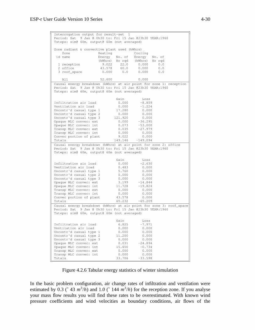
ESP-r User Guide Version 10 Series 4-30
Interrogation output for result-set 1Period: Sat 9 Jan @ 0h30 to: Fri 15 Jan @23h30 YEAR:1960Tsteps: sim@ 60m, output@ 60m (not averaged)
Zone radiant & convective plant used (kWhrs)Zone Heating Cooling
id name Energy No. of Energy No. of(kWhrs) Hr rqd (kWhrs) Hr rqd
1 reception 9.022 22.0 0.000 0.02 office 43.578 60.0 0.000 0.03 roof_space 0.000 0.0 0.000 0.0
All 52.600 0.000
Causal energy breakdown (kWhrs) at air point for zone 1: receptionPeriod: Sat 9 Jan @ 0h30 to: Fri 15 Jan @23h30 YEAR:1960Tsteps: sim@ 60m, output@ 60m (not averaged)
Gain LossInfiltration air load 0.000 -8.859Ventilation air load 0.000 -1.224Uncontr‘d casual type 1 17.280 0.000Uncontr‘d casual type 2 0.000 0.000Uncontr‘d casual type 3 121.920 0.000Opaque MLC convec: ext 0.000 -36.295Opaque MLC convec: int 0.073 -53.000Transp MLC convec: ext 0.035 -27.979Transp MLC convec: int 0.000 0.000Convec portion of plant 9.022 0.000Totals 149.146 -149.094
Causal energy breakdown (kWhrs) at air point for zone 2: officePeriod: Sat 9 Jan @ 0h30 to: Fri 15 Jan @23h30 YEAR:1960Tsteps: sim@ 60m, output@ 60m (not averaged)
Gain LossInfiltration air load 0.000 -2.630Ventilation air load 0.483 0.000Uncontr‘d casual type 1 5.760 0.000Uncontr‘d casual type 2 0.000 0.000Uncontr‘d casual type 3 0.000 0.000Opaque MLC convec: ext 3.199 -14.844Opaque MLC convec: int 11.728 -19.824Transp MLC convec: ext 0.000 0.000Transp MLC convec: int 0.000 0.000Convec portion of plant 43.578 0.000Totals 65.232 -65.209
Causal energy breakdown (kWhrs) at air point for zone 3: roof_spacePeriod: Sat 9 Jan @ 0h30 to: Fri 15 Jan @23h30 YEAR:1960Tsteps: sim@ 60m, output@ 60m (not averaged)
Gain LossInfiltration air load 6.825 -7.971Ventilation air load 0.000 0.000Uncontr‘d casual type 1 0.000 0.000Uncontr‘d casual type 2 11.200 0.000Uncontr‘d casual type 3 0.000 0.000Opaque MLC convec: ext 0.031 -24.894Opaque MLC convec: int 15.650 -0.734Transp MLC convec: ext 0.000 0.000Transp MLC convec: int 0.000 0.000Totals 33.706 -33.598
Figure 4.2.6 Tabular energy statistics of winter simulation
In the basic problem configuration, air change rates of infiltration and ventilation wereestimated by 0.3 (˜ 43 m3/h) and 1.0 (˜ 144 m3/h) for the reception zone. If you analyseyour mass flow results you will find these rates to be overestimated. With known windpressure coefficients and wind velocities as boundary conditions, air flows of the
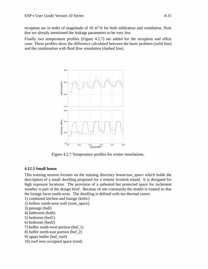
ESP-r User Guide Version 10 Series 4-31
reception are in order of magnitude of 10 m3/h for both infiltration and ventilation. Notethat we already mentioned the leakage parameters to be very low.
Finally two temperature profiles (Figure 4.2.7) are added for the reception and officezone. These profiles show the difference calculated between the basic problem (solid line)and the combination with fluid flow simulation (dashed line).
9.0 10.0 11.0 12.0 13.0 14.0daynumber
0.0
10.0
20.0
30.0
airt
emp.
off
ice
0.0
10.0
20.0
30.0
and
rece
ptio
n
Figure 4.2.7 Temperature profiles for winter simulations.
4.12.3 Small house
This training session focuses on the training directory house/sun_space which holds thedescription of a small dwelling proposed for a remote Scottish island. It is designed forhigh exposure locations. The provision of a unheated but protected space for inclementweather is part of the design brief. Because of site constraints the model is rotated so thatthe lounge faces south-west. The dwelling is defined with ten thermal zones:1) combined kitchen and lounge (kitliv)2) hollow south-west wall (west_space)3) passage (hall)4) bathroom (bath)5) bedroom (bed1)6) bedroom (bed2)7) buffer south-west portion (buf_1)8) buffer north-east portion (buf_2)9) upper buffer (buf_roof)10) roof over occupied space (roof)

ESP-r User Guide Version 10 Series 4-32
The dwelling has deep window rev eals and its orientation suggests that a detailed treat-ment of shading and solar penetration is called for. To this end obstruction blocks definethe deep window rev eals in the bedrooms and kitchen/lounge and correctly limit sunlightentering the dwelling.
The model uses seasonally adjusted mass flow networks to predict air movements. Thereare timed extract fans in the kitchen and bathroom as well as logic to open the windowsduring particular hours and if internal temperatures rise above a particular point. This isdefined in the configuration control file.
The subdivision of the buffer space into three thermal zones allows warm air to rise intothe upper space but for the front and back of the space to evolve different temperatures asa result of solar radiation patterns. This requires that ‘fictitious’ boundaries be usedbetween the zones and project based optical properties and multilayer constructiondatabases have been created.
Of interest is the treatment of the south-west wall of the lounge as a separate thermalzone rather than as a conventional multilayer construction. The reason for this is thelarge void (300mm) within this wall which, thus described, will have a more detailedtreatment of radiant exchanges.
There are two configuration files, house_win.cfg which is used for winter simulations andhouse_sum.cfg for summer simulations. Similarly there are two mass flow networkdescriptions (ss_sum.afn and ss_win.afn for summer and winter respectively). The con-trol file ss_win.ctl should be used with winter simulations and ss_sum.ctl with summersimulations.
To browse the fluid flow network associated with a given problem use the appropriatecommand of the project manager. The winter fluid flow network with the correspondingcontrol functions is listed below.
13 7 18 1.000 (nodes, components, connections, wind reduction)Node Fld. Type Height Temperature Data_1 Data_2liv 1 0 1.2000 20.000 0. 62.500hall 1 0 1.2000 20.000 0. 40.960bath 1 0 1.2000 20.000 0. 26.200bed1 1 0 1.2000 20.000 0. 48.980bed2 1 0 1.2000 20.000 0. 48.980buf_1 1 0 1.2000 20.000 0. 113.56buf_ro 1 0 4.3000 15.000 0. 211.45ext_we 1 3 1.2000 0. 5.0000 270.00ext_ea 1 3 1.2000 0. 5.0000 90.000roof_w 1 3 4.3000 0. 8.0000 270.00roof_e 1 3 4.3000 0. 8.0000 90.000north 1 3 2.0000 0. 1.0000 0.buf_2 1 0 1.2000 20.000 0. 60.000Comp Type C+ L+ Descriptiondoor 130 5 0 Specific air flow door m = rho.f(W,H,dP)
1.00000 0.300000 2.10000 1.50000 0.920000door25 130 5 0 Specific air flow door m = rho.f(W,H,dP)
1.00000 0.300000 2.10000 0.50000 0.920000horop 110 2 0 Specific air flow opening m = rho.f(A,dP)
1.00000 3.00000bathex 460 3 0 Fixed flow rates controller
1.00000 0. 2.20000E-02kitex 460 3 0 Fixed flow rates controller
1.00000 0. 1.40000E-02crck 120 3 0 Specific air flow crack m = rho.f(W,L,dP)
1.00000 1.00000E-02 1.00000

ESP-r User Guide Version 10 Series 4-33
crckl 120 3 0 Specific air flow crack m = rho.f(W,L,dP)1.00000 2.00000E-02 1.00000
+Node dHght -Node dHght Comp Snod1 Snod2ext_we 0.000 liv 0.000 crckext_we 0.000 buf_1 0.000 crckext_ea 0.000 bed2 0.000 crckext_ea 0.000 bed1 0.000 crckext_ea 0.000 buf_2 0.000 crckliv 0.000 buf_1 0.000 crcklliv 0.000 hall 0.000 door25hall 0.000 buf_1 0.000 crcklhall 0.000 bath 0.000 door25hall 0.000 bed1 0.000 door25hall 0.000 bed2 0.000 door25buf_1 0.000 buf_ro 0.000 horopbuf_2 1.000 buf_ro -1.000 horopbuf_1 0.000 buf_2 0.000 doorbuf_ro 0.000 roof_w 0.000 crcklbuf_ro 0.000 roof_e 0.000 crcklliv 0.000 north 0.000 kitexbath 0.000 north 0.000 bathex
* Mass Flowopening control # flow descr
2 # No. of controls* Control mass# measures mass flow node or connection.
-4 0 0 0 # sensor data# actuates mass flow component: 4 bathex
-4 4 1 # actuator data1 # No. day types1 365 # valid Sun 1 Jan - Sun 31 Dec5 # No. of periods in day1 0 0.000 # ctl type (dry bulb > flow), law (on / off), start @2. # No. of data items
30.000 1.0001 0 7.000 # ctl type (dry bulb > flow), law (on / off), start @2. # No. of data items
0.000 1.0001 0 9.000 # ctl type (dry bulb > flow), law (on / off), start @2. # No. of data items
30.000 1.0001 0 17.000 # ctl type (dry bulb > flow), law (on / off), start @2. # No. of data items
10.000 1.0001 0 19.000 # ctl type (dry bulb > flow), law (on / off), start @2. # No. of data items
30.000 1.000bath north bathex bath* Control mass# measures mass flow node or connection.
-4 0 0 0 # sensor data# actuates mass flow component: 5 bathpm
-4 5 1 # actuator data1 # No. day types1 365 # valid Sun 1 Jan - Sun 31 Dec5 # No. of periods in day1 0 0.000 # ctl type (dry bulb > flow), law (on / off), start @2. # No. of data items
30.000 1.0001 0 7.000 # ctl type (dry bulb > flow), law (on / off), start @2. # No. of data items
0.000 1.0001 0 8.000 # ctl type (dry bulb > flow), law (on / off), start @2. # No. of data items
30.000 1.0001 0 17.000 # ctl type (dry bulb > flow), law (on / off), start @2. # No. of data items
0.000 1.0001 0 18.000 # ctl type (dry bulb > flow), law (on / off), start @2. # No. of data items
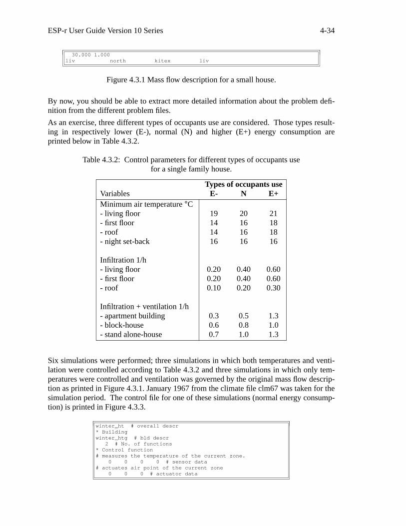
ESP-r User Guide Version 10 Series 4-34
30.000 1.000liv north kitex liv
Figure 4.3.1 Mass flow description for a small house.
By now, you should be able to extract more detailed information about the problem defi-nition from the different problem files.
As an exercise, three different types of occupants use are considered. Those types result-ing in respectively lower (E-), normal (N) and higher (E+) energy consumption areprinted below in Table 4.3.2.
Table 4.3.2: Control parameters for different types of occupants usefor a single family house.
Types of occupants useVariables E- N E+Minimum air temperature °C- living floor 19 20 21- first floor 14 16 18- roof 14 16 18- night set-back 16 16 16
Infiltration 1/h- living floor 0.20 0.40 0.60- first floor 0.20 0.40 0.60- roof 0.10 0.20 0.30
Infiltration + ventilation 1/h- apartment building 0.3 0.5 1.3- block-house 0.6 0.8 1.0- stand alone-house 0.7 1.0 1.3
Six simulations were performed; three simulations in which both temperatures and venti-lation were controlled according to Table 4.3.2 and three simulations in which only tem-peratures were controlled and ventilation was governed by the original mass flow descrip-tion as printed in Figure 4.3.1. January 1967 from the climate file clm67 was taken for thesimulation period. The control file for one of these simulations (normal energy consump-tion) is printed in Figure 4.3.3.
winter_ht # overall descr* Buildingwinter_htg # bld descr
2 # No. of functions* Control function# measures the temperature of the current zone.
0 0 0 0 # sensor data# actuates air point of the current zone
0 0 0 # actuator data
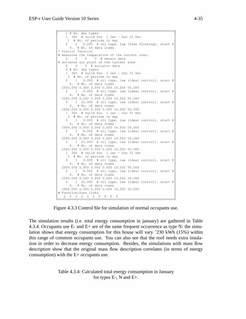
ESP-r User Guide Version 10 Series 4-35
1 # No. day types1 365 # valid Sun 1 Jan - Sun 31 Dec1 # No. of periods in day
0 2 0.000 # ctl type, law (free floating), start @0. # No. of data items
* Control function# measures the temperature of the current zone.
0 0 0 0 # sensor data# actuates air point of the current zone
0 0 0 # actuator data0 # No. day types1 365 # valid Sun 1 Jan - Sun 31 Dec3 # No. of periods in day
0 1 0.000 # ctl type, law (ideal control), start @6. # No. of data items
2000.000 0.000 0.000 0.000 16.000 50.0000 1 6.000 # ctl type, law (ideal control), start @6. # No. of data items
2000.000 0.000 0.000 0.000 19.000 50.0000 1 22.000 # ctl type, law (ideal control), start @
6. # No. of data items2000.000 0.000 0.000 0.000 16.000 50.0001 365 # valid Sun 1 Jan - Sun 31 Dec3 # No. of periods in day
0 1 0.000 # ctl type, law (ideal control), start @6. # No. of data items
2000.000 0.000 0.000 0.000 16.000 50.0000 1 8.000 # ctl type, law (ideal control), start @6. # No. of data items
2000.000 0.000 0.000 0.000 19.000 50.0000 1 23.000 # ctl type, law (ideal control), start @
6. # No. of data items2000.000 0.000 0.000 0.000 16.000 50.0001 365 # valid Sun 1 Jan - Sun 31 Dec3 # No. of periods in day
0 1 0.000 # ctl type, law (ideal control), start @6. # No. of data items
2000.000 0.000 0.000 0.000 16.000 50.0000 1 8.000 # ctl type, law (ideal control), start @6. # No. of data items
2000.000 0.000 0.000 0.000 19.000 50.0000 1 22.000 # ctl type, law (ideal control), start @
6. # No. of data items2000.000 0.000 0.000 0.000 16.000 50.000
# Function:Zone links2 0 2 2 2 2 0 0 0 0
Figure 4.3.3 Control file for simulation of normal occupants use.
The simulation results (i.e. total energy consumption in january) are gathered in Table4.3.4. Occupants use E- and E+ are of the same frequent occurrence as type N: the simu-lation shows that energy consumption for this house will vary ˜230 kWh (15%) withinthis range of common occupants use. You can also see that the roof needs extra insula-tion in order to decrease energy consumption. Besides, the simulations with mass flowdescription show that the original mass flow description correlates (in terms of energyconsumption) with the E+ occupants use.
Table 4.3.4: Calculated total energy consumption in Januaryfor types E-, N and E+.

ESP-r User Guide Version 10 Series 4-36
ENERGY CONSUMPTION [kWhr]Zone E- E-(mfs) N N(mfs) E+ E+(mfs)
- kitchen 54 127 97 138 151 153- hall 126 141 152 146 178 147- bath 8 2 13 1 24 7- bed1 25 47 52 64 84 83- bed2 28 51 52 65 83 82- roof 1136 1117 1252 1225 1320 1293
Total consumption 1377 1484 1618 1638 1839 1764
Succeeding simulations can be performed to determine the variation in summer’s coolingenergy.
4.12.4 Large house
Increasing the complexity of the models we now turn to the training directory house/svphwhich is an example of a moderate size dwelling based on a direct gain house in MiltonKe ynes. It has become a de facto modelling standard within the UK.
The directory structure, as for other exemplars described above, is an example of usingseveral subdirectories to hold different portions of the problem definition. The benefit ofthis is that each directory has only a limited number of files.
training/house/svph‘-----configuration (cfg)‘-----control (ctl)‘-----networks‘-----zones
4.12.5 Test cells
To be completed.
4.12.6 Special focus
There are a number of specialised facilities within ESP-r which are provided for expertusers and those who require additional detail in their simulation work. Several examplesare given in the exemplars. One example relates to the thermophysical property replace-ment facility.
It is based on the simple_building problem. The situation modelled in constr/tp_sub isthat the conductivity of the glass wool in some of the external walls is increased when theinternal air temperature rises above a certain temperature (20°C). This is obviously not areal situation, but a similar situation could occur if the conductivity of a particular con-structional material was sensitive to temperature.
An additional entry (glasswool_mod, #282) has been made in the primitives database(tp_subs.pdb). This is similar to glasswool (#211) but with increased conductivity. A new

ESP-r User Guide Version 10 Series 4-37
entry has also been made in the multi-constructional database (tp_subc.mlc) which is forext_wall_mod. This is the same as for the entry for extern_wall except that it uses themodified properties of glasswool.
The control file demonstrates the activation of the replacement constructions. For thespace named reception, constructions ’south’, ’east’ and ’north’, and for the office space,constructions ’North_w’ and ’West_w’, use the replacement construction whenever theroom temperature exceeds 20°C. In the control file, control function 1 (assigned to thereception) has a ’nested’ control function 3 which gives details of the thermophysicalproperty control. Similarly, control function 2 (for the office) has a ’nested’ control func-tion 4.
4.12.7 Office block
This session switches the focus to full scale commercial buildings with a two lev el officeblock located in the north-east of Scotland. The 17-zone model makes use of mass flowsimulation and opening of windows to control summer overheating. Images of the prob-lem (in gif format) are included in the images directory.
To access the problem definitions go into the configuration directory. Within the configu-ration directory is a file office.log which should be viewed via UNIX or project managerfacilities.
As this is a large problem it is recommended that simulations be kept to a few days. Insummer simulations you will note that the zone temperatures are to some extent a func-tion of wind velocity and direction.
4.12.8 Plant
To be completed.

Section FiveTheoretical basis and validity
of theESP-r system
Contents
5.0 Introduction5.1 Theoretical basis5.2 Validity5.3 Model value

ESP-r Manual: Version 10 Series 5-2
5.0 Introduction
A comprehensive description of ESP-r’s mathematical model, and the verification testsapplied to it, would occupy much space, and so is not undertaken here. Instead, ESP-r’stheory is stated conceptually and the various publications covering theory and validity arereferenced.
5.1 Theoretical basis
ESP-r uses an advanced numerical method to integrate the various equation types (alge-braic, ordinary differential and partial differential) which can be used to represent heatand mass balances within buildings. The system is non-building type specific and canhandle any plant system as long as the necessary component models are installed in theplant components’ database. Components, if missing, can be added by a user so that theybecome available for selection to participate in any multi-component plant configuration.But since component models must conform to state-space formulations, new componentderivation and insertion is often a non-trivial task - the price of plant modelling in thetransient domain.
In addition to the usual energy analysis features (comfort assessment, condensationchecks, and the like), ESP-r can handle the spectral analysis of glazing systems whichinclude thin films, time varying shading caused by site obstructions, solar ray tracing,pressure and buoyancy induced air movement and complex, distributed control systems.
A conceptual explanation of ESP-r’s calculation technique would go something like:
The system offers a way to rigorously analyse the energy performance of a buildingand its environmental control systems. For each observable energy flow-path in thereal world, ESP-r has a corresponding mathematical structure. Within a simula-tion, a special numerical technique ensures that all flow-paths evolve simultane-ously to fully preserve the important spatial and temporal relationships. Statedbriefly, ESP-r will accept some building/plant description in terms of 3-D geome-try, construction, usage and control. This continuous system is then made discreteby division into many small, but finite, volumes of space - perhaps as many as10,000 for a medium sized building. These finite volumes will represent the vari-ous regions of the building and plant within and between which energy and masscan flow. Throughout any subsequent simulation, ESP-r will track the energy andmass balance for all finite volumes as they evolve under the influence of the systemboundary conditions (climate & control) and the constraints imposed by the inter-volume links. This technique ensures that all regions of the building are correctlyconnected across space and time and so any excitation at some point in space ortime will have the correct causal effect.
The following publication details the theory and structure of ESP-r:
Clarke J A, Energy Simulation in Building Design, 2nd Edition, Butterworth-Heinemann, Oxford, 2001.
ESP-r’s mathematical approach is derived and the numerical method used to achieve therepetitive and simultaneous integration of each flow-path over time is explained.
As described in Section One, ESRU maintains a list of bibliographic references, describ-ing much of ESP-r’s technical detail and philosophy. This list is available from ESRU on

ESP-r Manual: Version 10 Series 5-3
request.
5.2 Validity
Many model users do not yet appreciate the complexities of large scale energy model val-idation. Indeed it is probably true that absolute declarations of validity will never be pos-sible. This is because the data used to describe the problem is itself subject to great uncer-tainty, and because the combinatorial links between input assumptions, logic representa-tions, mathematical techniques and output interpretations is very large. It is now widelyrecognised that confidence levels can only be improved by dev eloping verificationmethodologies and by repeatedly undertaking studies which aim to verify discrete aspectsof a model under different operating conditions. In this respect ESP-r has a good trackrecord. It was/is a participant model in the International Energy Agency’s Annex 1, 4 and10 projects concerned with inter-model and empirical model verification in both buildingand systems simulation modes. ESP-r has also been tested by several organisations exter-nal to ESRU and found to agree well with known analytical solutions and monitored datasets. On the basis of these findings the program has been declared the European Refer-ence Model for Passive Solar Architectural Design and has been examined extensively ina SERC (now EPSRC) funded research project to develop a model verification methodol-ogy. ESP-r has also been well tested within the EC’s PASSYS project. Several validationreports have been generated at ESRU and elsewhere. iA summary can be obtained by filetransfer from: <ftp://ftp.strath.ac.uk/Esru_public/documents/validation.pdf>.
5.3 Model value
ESP-r is a state-of-the-art model which allows the rapid performance assessment of pro-posed building designs incorporating traditional and/or advanced energy features. For thefirst time, a user is able to conduct a high integrity, first principle appraisal whilst mod-elling all aspects of the energy subsystem simultaneously and in the transient domain.Indeed many design problems (for example fabric design, comfort or condensationassessment, control system appraisal, etc.) can only be meaningfully assessed when con-sidered in this manner, as one portion of some complex set of interactions. That is, apiecemeal approach, in which a particular region is considered in isolation, is totallyinappropriate and often misleading. At an early design stage a model such as ESP-r isparticularly powerful since it can be used to quantify the performance impact of the site,the building geometry and construction; all factors which have considerable impact onoperational performance and costs. Then, at the more detailed design stage, the modelallows the designer to focus on issues of control and comfort.