Equilibrium Tuition, Applications, Admissions and ...

Equilibrium Tuition, Applications, Admissions and

Enrollment in the College Market�

Chao Fuy

October, 2011

Abstract

I develop and estimate a structural equilibrium model of the college market. Stu-

dents, having heterogeneous abilities and preferences, make college application deci-

sions, subject to uncertainty and application costs. Colleges, observing only noisy

measures of student ability, choose tuition and admissions policies to compete for more

able students. Tuition, applications, admissions and enrollment are joint outcomes

from a subgame perfect Nash equilibrium. I estimate the structural parameters of

the model using data from the National Longitudinal Survey of Youth 1997, via a

three-step procedure to deal with potential multiple equilibria. In counterfactual ex-

periments, I use the model �rst to examine the extent to which college enrollment can

be increased by expanding the supply of colleges, and then to assess the importance of

various measures of student ability.

Keywords: College market, tuition, applications, admissions, enrollment, discrete choice,

market equilibrium, multiple equilibria, estimation

�I am immensely grateful to Antonio Merlo, Philipp Kircher, and especially to my main advisor KennethWolpin for invaluable guidance and support. I thank Kenneth Burdett, Steven Durlauf, Aureo De Paula,Hanming Fang, John Kennan, George Mailath, Guido Menzio, Andrew Postlewaite, Frank Schorfheide, ChrisTaber, Petra Todd and Xi Weng for insightful comments and discussions. Comments from participants ofthe NBER 2010 Summer Labor Studies, UPENN Search and Matching Workshop were also helpful. Allerrors are mine.

yDepartment of Economics, University of Wisconsin, Madison, WI 53706, USA. Email: [email protected].

1

1 Introduction

Both the level of college enrollment and the composition of college student bodies continue

to be issues of widespread scholarly interest as well as the source of much public policy

debate. In this paper, I develop and structurally estimate an equilibrium model of the college

market. It provides insights into the determination of the population of college enrollees and

permits quantitative evaluation of the e¤ects of counterfactual changes in the features of the

college market. The model interprets the allocation of students in the college market as an

equilibrium outcome of a decentralized matching problem involving the entire population of

colleges and potential applicants.1 As a result, counterfactuals that directly involve only a

subset of the college or student population can produce equilibrium e¤ects for all market

participants. My paper thus provides a mechanism for assessing the market equilibrium

consequences of changes in government policies on higher education.

While the idea of modeling college matching as a market equilibrium problem is not new,

this paper makes advances relative to the current literature by simultaneously modeling

three aspects of the college market that are plausibly regarded as empirically important

and incorporating them into the empirical analysis. The three aspects are: 1) Application

is costly to the student. Besides application fees, a student has to spend time and e¤ort

gathering and processing information and preparing application materials. Moreover, she

also incurs nontrivial psychic costs such as the anxiety felt while waiting for admissions

results. 2) Students di¤er in their abilities and preferences for colleges.2 3) While trying to

attract and select more able students, colleges can only observe noisy measures of student

ability, such as student test scores and essays. As a result, both sides of the market face

uncertainties: for the student, admissions are uncertain, which, together with the cost of

application, leads to a non-trivial portfolio problem for her: how many and which, if any,

colleges to apply to? For the college, the yield of each admission and the quality of a potential

enrollee are both uncertain. The inference of these has to account for students�strategies.

Colleges�policies are also interdependent because students�application portfolios and their

enrollment depend on the policies of all colleges.

I model three stages of the market. First, colleges simultaneously announce their tuition.

Second, students make application decisions and colleges simultaneously choose their ad-

missions policies. Third, students make their enrollment decisions. My model incorporates

tuition, applications, admissions and enrollment as joint outcomes from a subgame perfect

Nash equilibrium (SPNE). SPNE in this model need not be unique. Multiplicity may arise

1In this paper, colleges refer to four-year colleges; students (potential applicants) refer to high schoolgraduates.

2Throughout the paper, student ability refers to her readiness for college.

1

from two sources: 1) multiple common self-ful�lling expectations held by the student about

admissions policies, and 2) the strategic interplay among colleges.3

To estimate the model with potentially multiple equilibria, I extend the estimation strat-

egy of Moro (2003) and estimate the model in three steps.4 The �rst two steps recover

all the structural parameters involved in the application-admission subgame without having

to impose any equilibrium selection rule. In particular, each application-admission equilib-

rium can be uniquely summarized in the set of probabilities of admission to each college

for di¤erent types of students. The �rst step, using simulated maximum likelihood, treats

these probabilities as parameters and estimates them along with fundamental student-side

parameters in the student decision model, thereby identifying the equilibrium that generated

the data. The second step, based on a simulated minimum distance estimation procedure,

recovers the college-side parameters by imposing each college�s optimal admissions policy.

Step three recovers the remaining parameters by matching colleges�optimal tuition with the

data tuition.

To implement the empirical analysis, I use data from the National Longitudinal Sur-

vey of Youth 1997 (NLSY97), which provides detailed information on student applications,

admissions, �nancial aid and enrollment. Tuition information comes from the Integrated

Postsecondary Education Data System.

Some of my major �ndings are as follows: �rst, students not only attach di¤erent values

to the same college, but also rank various colleges and the non-college option di¤erently.

That is, there is not a single best college for all, nor is attending college better than the non-

college option for all. As a result, my �rst counterfactual experiment �nds that increasing

the supply of colleges has very limited e¤ect on college attendance. In particular, when the

lower-ranked public colleges are expanded, at most 2:1% more students can be drawn into

colleges, although the enlarged colleges adopt an open admissions policy and lower their

tuition to almost zero. Therefore, neither tuition cost nor the number of available slots is

a major obstacle to college access. A large group of students, mainly low-ability students,

prefer the outside option over any of the college options.

Second, there are signi�cant amounts of noise in various types of ability measures and

di¤erent types of measures complement one another. In particular, relative to measures such

3Models with multiple equilibria do not have a unique reduced form and this indeterminacy poses practicalestimation problems. In direct maximum likelihood estimation of such models, one should maximize thelikelihood not only with respect to the structural parameters but also with respect to the types of equilibriathat may have generated the data. The latter is a very complicated task and can make the estimationinfeasible.

4Moro (2003) estimates a statistical discrimination model in which only one side of the market is strategic.I show how the extended strategy can be used to estimate a model in which both sides of the market arestrategic, and hence, the second source of multiple equilibria arises.

2

as student essays, test scores (SAT ) are more e¤ective in distinguishing the lowest-ability

students from the rest, but are less e¤ective in singling out high-ability students.5 My second

counterfactual experiment assesses the importance of the non-test-score measures of student

ability by eliminating them in the admissions process. Without such additional information,

colleges draw on higher tuition to help screen students. Enrollee ability drops in all colleges,

especially in the top college groups. Despite the increased tuition, the gain from being

mixed with others outweighs the loss for the lowest-ability students. However, all the other

students su¤er and the average student welfare decreases by $1; 325. The highest-ability

students su¤er the most with a loss of about $5; 000:

The third counterfactual experiment examines the equilibrium impacts of dropping SAT

in the admissions process, as urged by some critics. Among other reasons, these critics blame

SAT for inhibiting the access to college education for students from low-income families,

who typically have low test scores. As a result of dropping SAT , the fraction of low-income

students does increase in top colleges. In particular, the mean family income among enrollees

drop by over $10; 000 in top private colleges. However, this is accompanied by increased

tuition and decreased enrollee ability in these colleges.

Although this paper is the �rst to estimate a market equilibrium model that incorpo-

rates tuition setting, applications, admissions and enrollment, it builds on various studies

on similar topics. For example, Manski and Wise (1983) use nonstructural approaches to

study various stages of the college admissions problem separately in a partial equilibrium

framework. Most relevant to this paper, they �nd that applicants do not necessarily prefer

the highest quality school.6 Arcidiacono (2005) develops and estimates a structural model

to address the e¤ects of college admissions and �nancial aid rules on future earnings. In a

dynamic framework, he models student�s application, enrollment and choice of college major

and links education decisions to future earnings.

While an extensive empirical literature focuses on student decisions, little research has

examined the college market in an equilibrium framework. One exception is Epple, Romano

and Sieg (2006). In their paper, students di¤er in family income and ability (perfectly mea-

sured by SAT ) and make a single enrollment decision.7 Taking, as given, its endowment

and gross tuition level, each college chooses its �nancial aid and admissions policies to max-

imize the quality of education provided to its students. Their model provides an equilibrium

5In this paper, SAT is used as a generic term for tests such as SAT and ACT:6Some examples of papers that focus on the role of race in college admissions include Bowen and Bok

(1998), Kane (1998) and Light and Strayer (2002).7In their paper, the application decision is not modeled. It is implicitly assumed that either application

is not necessary for admission, or all students apply to all colleges. Accordingly, their empirical analysis isbased on a sample of �rst-year college students.

3

characterization of colleges�pricing strategies, where colleges with higher endowments enjoy

greater market power and provide higher-quality education. With complete information, no

uncertainty and no unobserved heterogeneity, their model predicts that students with the

same SAT and family income would have the same admission, �nancial aid and enrollment

outcomes. The authors assume measurement errors in SAT and family income, which are

found to be large in order to accommodate data variations.8

This paper departs from Epple, Romano and Sieg (2006) in several respects: 1) The

college market is subject to information friction and uncertainty: colleges can only observe

noisy measures of student ability, and they do not observe student preferences. As a result,

colleges are faced with complex inference problems in making their admissions decisions.

Meanwhile, application becomes a non-trivial problem for the student, as is manifested by

the popularity of various application guide programs. Both colleges and students will adjust

their behavior according to how much information is available on the market. Consequently,

evaluating the severity of the information friction is important for predicting the equilibrium

e¤ects of various counterfactual education policies. 2) Student application decisions di¤er

substantially. For example, over 50% of high school graduates do not apply to any college.

However, the college market includes not only those who do apply, but all potential college

applicants. Alternative education policies will a¤ect not only where applicants are enrolled,

but also who will apply at the �rst place. Therefore, to evaluate the e¤ects of these policies,

it is necessary to understand the application decisions (including non application) made

by all students and how these decisions interact with colleges�decisions. 3) Students have

di¤erent abilities and preferences for colleges, which are unobservable to econometricians.

Arguably, such heterogeneity may be the key force underlying data variations unexplained

by observables. Hence it is important to incorporate them in the model. As the �rst two

structural papers that study college market equilibrium, Epple, Romano and Sieg (2006)

and this paper complement one another: the former provides a more comprehensive view

on colleges�pricing strategy, while the latter endogenizes student application as part of the

equilibrium in a frictional market.

Theoretically, I build on the work by Chade, Lewis and Smith (2011), who model the

decentralized matching of students and two colleges. Students, with heterogeneous abilities,

make application decisions subject to application costs and noisy evaluations. Colleges com-

pete for better students by setting admissions standards for student signals.9 As part of its

contribution, my paper quanti�es the signi�cance of the two key elements of Chade, Lewis

8The authors note that "the model may not capture some important aspects of admission and pricing."(page 911)

9Nagypál (2004) analyzes a model in which colleges know student types, but students themselves canonly learn their type through normally distributed signals.

4

and Smith (2011): information friction and application costs. Moreover, I extend Chade,

Lewis and Smith (2011) to account for some elements that are important, as acknowledged

by the authors, to understand the real-world problem. On the student side, �rst, students

are heterogeneous in their preferences for colleges as well as in their abilities, both of which

are unknown to the colleges. Second, I allow for two noisy measures of student ability. One

measure, as the signal in Chade, Lewis and Smith (2011), is subjective and its assessment is

known only to the college. A typical example of this type of measure is the student essay.

The other measure is the objective test score, which is known both to the student and to the

colleges she applies to, and may be used strategically by the student in her applications.10

Third, in addition to the admission uncertainty caused by noisy evaluations, students are

subject to post-application shocks. These shocks incorporate new information for the stu-

dent before she makes her enrollment decision. For example, the amount of �nancial aid

she can obtain is not known with certainty upon application. Moreover, during the months

between application and enrollment, a student may learn more about the colleges and she

may also experience unexpected family and/or job prospects.11 Empirically, these shocks are

necessary to explain "seemingly sub-optimal" behaviors such as an applicant choosing not

to attend any college after being admitted. On the college side, I model multiple colleges,

which compete against each other via tuition as well as admissions policies.12

The rest of the paper is organized as follows: Section 2 lays out the model. Section 3

explains the estimation strategy, followed by a brief discussion of identi�cation. Section 4

describes the data. Section 5 presents empirical results, including parameter estimates and

model �t. Section 6 describes the counterfactual experiments. The last section concludes

the paper. The appendix contains some details and additional tables.

2 Model

2.1 Primitives

This subsection lays out the environment of the college market that features costly applica-

tion and incomplete information.

10For example, a low-ability student with a high SAT score may apply to top colleges to which she wouldnot otherwise apply; a high-ability student with a low SAT score may apply less aggressively than she wouldotherwise.11For enrollment in the fall semester starting from September, the typical application deadline is in January.12As a price of these extensions, it is infeasible to obtain an analytical or graphical characterization of the

equilibrium as in Chade, Lewis and Smith (2011).

5

2.1.1 Players

There are J colleges, indexed by j = 1; 2; :::J . In the following, J will also denote the set

of colleges. A college�s payo¤ depends on the total expected ability of its enrollees and its

tuition revenue. To maximize its payo¤, each college has the latitude to choose its tuition and

admissions policies, subject to its �xed capacity constraint �j, where �j > 0 andXj2J

�j < 1,

the total measure of students.

There is a continuum of students, making college application and enrollment decisions.

Students di¤er in their family backgrounds (B), SAT , abilities and preferences for colleges.13

The various components of student characteristics are drawn from some joint distribution,

unknown to the econometrician, who observes neither students�abilities nor their preferences.

2.1.2 Application Cost

Application is costly to the student. The cost of application, denoted as C(�); is a non-parametric function of the number of applications sent. C(n + 1) � C(n) > 0; for any

n 2 f1; :::; J � 1g.

2.1.3 Financial Aid

A student may obtain �nancial aid that helps to fund her attendance in any college, and she

may also obtain college-speci�c �nancial aid. The amounts of various �nancial aid depend

on the student�s family background and SAT , via �nancial aid functions fj(B; SAT ), for

j = 0; 1:::J , with 0 denoting the general aid and j denoting college j-speci�c aid.14 In

reality, although guidelines are available for students to calculate the expected �nancial aid

she might obtain, the exact amount remains uncertain to her. To capture this uncertainty,

I allow the �nal realizations to be subject to post-application shocks � 2 RJ+1. � is i.i.d.N(0;�), where � is a diagonal matrix with �2�j denoting the variance of shock �j. The

realized �nancial aid for student i is given by

fji = maxffj(Bi; SATi) + �ji; 0g for j = 0; 1; ::J:13SAT can be low(1), medium(2) or high(3).14Ideally, a more complete model would endogenize tuition, applications, admissions, enrollment and �nan-

cial aid. Unfortunately, this involves great complications that will make the empirical analysis intractable.As a compromise, Epple, Romano and Sieg (2006) abstract from application decisions and hence the e¤ectsof college policies on the pool of applicants, so that they can better focus on college�s �nancial aid strategies.I carry out my analysis in a way that complements their work: I endogenize application decisions and allowcolleges to choose gross tuition while leaving �nancial aid exogenous, which indirectly a¤ects colleges�policiesvia its e¤ects on students�application and enrollment decisions. The development of a modeling frameworkthat combines the strengths of these two papers is a great challenge.

6

2.1.4 Student Preference

Student characteristics such as their abilities and preferences are unobservable to the econo-

metrician. They are modeled as follows: students are of di¤erent types (T ), where T is

correlated with (SAT;B) and distributed according to P (T jSAT;B). A student type T

consists of both ability and non-ability related characteristics, with T � (A;Z) : The �rst

component, A; represents a student�s ability, which can be low (1); medium (2) or high (3).

Meanwhile, some students may prefer big (public) universities that o¤er greater diversity

and a wider range of student activities; while some may prefer small (private) colleges where

they can get more personal attention from professors. Such heterogeneity is captured by

Z 2 f1; 2g.Students�preferences for colleges may di¤er systematically across types. In addition, each

student may still have her own idiosyncratic tastes for colleges that are not representative

of her type. For example, a student may prefer a particular type of colleges because her

parents used to attend such colleges. To capture both the systematic and the idiosyncratic

preference heterogeneities, students�preferences for colleges are modeled as a J-dimensional

random vector drawn from N(uT ;�), where uT is the mean preference for colleges among

type-T students and � is a diagonal matrix with �2�j denoting the variance of students�

idiosyncratic tastes for college j: In this way, a student�s preferences for di¤erent colleges are

allowed to be correlated in a nonparametric fashion via her type-speci�c preference uT :

Given tuition pro�le t � ftjgJj=1, the ex-post value of attending college j for student i isgiven by

uji(t) = (�tj + f0i + fji) + (ujTi + �ji) ; (1)

where tj is tuition for attending college j. The �rst parenthesis of (1) summarizes student

i�s net monetary cost to attend college j. Her expected payo¤, net of e¤ort cost, is captured

by: ujTi, type Ti-speci�c preference, and �ji, her idiosyncratic taste for college j. That is,

�i~N(0;�):

An outside option is always available to the student and its net expected value is nor-

malized to zero. During the months between application and enrollment, a student may

experience some unforeseen events that increase or decrease the value of her outside option.

For example, she may receive a good job o¤er that dominates the option of attending col-

lege. Such uncertainties are captured by a post-application random shock �, which is i.i.d.

N(0; �2�), and the ex-post value of the outside option is u0i = � i.

7

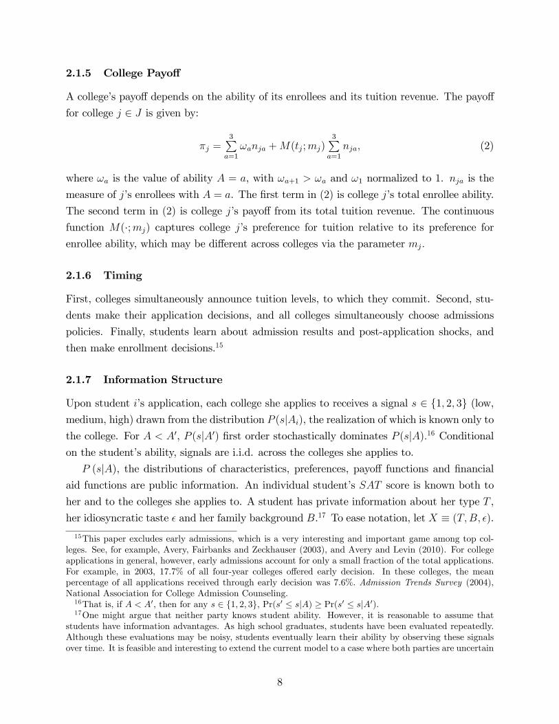
2.1.5 College Payo¤

A college�s payo¤ depends on the ability of its enrollees and its tuition revenue. The payo¤

for college j 2 J is given by:

�j =3Pa=1

!anja +M(tj;mj)3Pa=1

nja; (2)

where !a is the value of ability A = a, with !a+1 > !a and !1 normalized to 1. nja is the

measure of j�s enrollees with A = a. The �rst term in (2) is college j�s total enrollee ability.

The second term in (2) is college j�s payo¤ from its total tuition revenue. The continuous

function M(�;mj) captures college j�s preference for tuition relative to its preference for

enrollee ability, which may be di¤erent across colleges via the parameter mj:

2.1.6 Timing

First, colleges simultaneously announce tuition levels, to which they commit. Second, stu-

dents make their application decisions, and all colleges simultaneously choose admissions

policies. Finally, students learn about admission results and post-application shocks, and

then make enrollment decisions.15

2.1.7 Information Structure

Upon student i�s application, each college she applies to receives a signal s 2 f1; 2; 3g (low,medium, high) drawn from the distribution P (sjAi), the realization of which is known only tothe college. For A < A0, P (sjA0) �rst order stochastically dominates P (sjA):16 Conditionalon the student�s ability, signals are i.i.d. across the colleges she applies to.

P (sjA), the distributions of characteristics, preferences, payo¤ functions and �nancialaid functions are public information. An individual student�s SAT score is known both to

her and to the colleges she applies to. A student has private information about her type T ,

her idiosyncratic taste � and her family background B.17 To ease notation, let X � (T;B; �).15This paper excludes early admissions, which is a very interesting and important game among top col-

leges. See, for example, Avery, Fairbanks and Zeckhauser (2003), and Avery and Levin (2010). For collegeapplications in general, however, early admissions account for only a small fraction of the total applications.For example, in 2003, 17:7% of all four-year colleges o¤ered early decision. In these colleges, the meanpercentage of all applications received through early decision was 7:6%: Admission Trends Survey (2004),National Association for College Admission Counseling.16That is, if A < A0; then for any s 2 f1; 2; 3g; Pr(s0 � sjA) � Pr(s0 � sjA0):17One might argue that neither party knows student ability. However, it is reasonable to assume that

students have information advantages. As high school graduates, students have been evaluated repeatedly.Although these evaluations may be noisy, students eventually learn their ability by observing these signalsover time. It is feasible and interesting to extend the current model to a case where both parties are uncertain

8

After application, the student observes her post-application shocks. The following table

summarizes, in addition to the public information, what information is available to the

student and college j when they make decisions.

Information Set

Student College j

Application-Admission SAT;X = (T;B; �) SAT; sj

Enrollment SAT;X; �; � �

For any individual applicant, college j observes only her SAT and the signal she sends

to j, which are the basis on which the college makes admissions decisions. For the student,

the admission probability is a function of her SAT and ability (instead of signal), because

she cannot observe her signal but her ability governs her signal distribution.

2.2 Applications, Admissions and Enrollment

In this subsection, I solve the student�s problems backwards and the college�s admissions

problem, taking as given the tuition levels announced in the �rst stage of the game.

2.2.1 Enrollment Decision

Knowing her post-application shocks and admission results, student i chooses the best among

her outside option and admissions on hand, i.e., maxfu0i;fuji(t)gj2Oig, where Oi denotes theset of colleges that have admitted student i. Let

v(Oi; Xi; SATi; �i; � ijt) � maxfu0i;fuji(t)gj2Oig (3)

be the optimal ex-post value for student i, given admission set Oi; and denote the associated

optimal enrollment strategy as d(Oi; Xi; SATi; �i; � ijt).

2.2.2 Application Decision

Given her admissions probability pj(Ai; SATijt) to each college j, which depends on herability and SAT , the value of application portfolio Y � J for student i is

V (Y;Xi; SATijt) �XO�Y

Pr(OjAi;SATi; t)E [v(O;Xi; SATi; �i; � ijt)]� C(jY j); (4)

about student ability. In this paper, I focus on the special case, which captures the main idea of informationasymmetry of the type that I consider.

9

where the expectation is over shocks (�i; � i), and jY j is the size of portfolio Y .

Pr(OjAi;SATi; t) =Yj2O

pj(Ai; SATijt)Y

k2Y nO

(1� pk(Ai; SATijt))

is the probability that the set of colleges O � Y admit student i. The student�s application

problem is

maxY�J

fV (Y;Xi; SATijt)g: (5)

Let the optimal application strategy be Y (Xi; SATijt):

2.2.3 Admissions Policy

Given tuition, a college chooses its admissions policy to maximize its expected payo¤, subject

to its capacity constraint. Its optimal admissions policy must be a best response to other

colleges�admissions policies while accounting for students�strategic behavior. In particular,

observing only signals and SAT scores of its applicants, the college has to infer: �rst, the

probability that a certain applicant will accept its admission, and second, the expected ability

of this applicant conditional on her acceptance of the admission, both of which depend on

the strategies of all other players.18 For example, whether or not a student will accept college

j�s admission depends on whether she also applies to other colleges (which is unknown to

college j); and if so, whether or not she will be accepted by each of those colleges. In addition,

college j needs to integrate out the post-application shocks that may occur to the student.

In this paragraph, I describe how an optimal admissions policy is implemented. The rest

of Section 2.2.3 formalizes the problem, which can be skipped by readers not interested in the

details. To implement its admissions policy, college j will �rst rank its applicants with di¤er-

ent (s; SAT ) by their expected ability conditional on their acceptance of j�s admissions. All

applicants with the same (s; SAT ) are identical to the college and hence are treated equally.

Everyone in an (s; SAT ) group will be admitted if 1) this (s; SAT ) group is ranked highest

among the groups whose admissions are still to be decided, 2) their marginal contribution to

the college is positive, and 3) the expected enrollment of this group is no larger than college

j�s remaining capacity, where j�s remaining capacity equals �j minus the sum of expected

enrollment of groups ranked above. A random fraction of an (s; SAT ) group is admitted if

1) and 2) hold but 3) fails, where the fraction equals the remaining capacity divided by the

expected enrollment of this group. As a result, a typical set of admissions policies for the

18Conditioning on acceptance is necessary to make a correct inference about the student�s ability becauseof the potential "winner�s curse": the student might accept college j�s admission because she is of low abilityand is rejected by other colleges.

10

ranked (s; SAT ) groups, fej(s; SAT jt)g ; would be f1; :::; 1; "; 0; :::; 0g, with " 2 (0; 1) if thecapacity constraint is binding, and f1; :::; 1g if the capacity constraint is not binding or justbinding.

The following formally derives a college�s optimal admissions policy, readers not interested

in the details can skip to Section 2.2.4. Given tuition pro�le t, students�strategies Y (�); d(�)and other colleges�admissions policies e�j, college j solves the following problem:

maxej(�jt)

fXs;SAT

ej(s; SAT jt)�j(s; SAT jt; e�j; Y; d) j(s; SAT j�)�j(s; SAT j�) (6)

+M(tj;mj)Xs;SAT

ej(s; SAT jt)�j(s; SAT j�)�j(s; SAT j�)g

s:t:Xs;SAT

ej(s; SAT jt)�j(s; SAT j�)�j(s; SAT j�) � �j

ej(s; SAT jt) 2 [0; 1];

where ej(s; SAT jt) is college j�s admissions policy for its applicants with (s; SAT ),�j(s; SAT jt; e�j; Y; d) is the probability that such an applicant will accept college j�s ad-mission, j(s; SAT jt; e�j; Y; d) is the expected ability of such an applicant conditional onher accepting j�s admission, and �j(s; SAT jt; e�j; Y; d) is the measure of j�s applicants with(s; SAT ).19 Therefore, the �rst line of (6) is college j�s expected total enrollee ability; and

the second line is its expected total tuition revenue. The �rst order condition for problem

(6) is

j(s; SAT j�) +M(tj;mj)� �j + �0 � �1 = 0;

where �j is the multiplier associated with capacity constraint, i.e., the shadow price of a

slot in college j. �0 and �1 are adjusted multipliers associated with the constraint that

ej(s; SAT jt) 2 [0; 1]:20

If it admits an applicant with (s; SAT ) and the applicant accepts the admission, college

j must surrender a slot from its limited capacity, thus inducing the marginal cost �j. The

marginal bene�t is the expected ability of such an applicant conditional on her accepting

j�s admission plus her tuition contribution. Balancing between the marginal bene�t and the

marginal cost, the solution to college j�s admissions problem is characterized by:

ej(s; SAT jt)

8><>:= 1 if j(s; SAT j�) +M(tj;mj)� �j > 0

= 0 if j(s; SAT j�) +M(tj;mj)� �j < 0

2 [0; 1] if j(s; SAT j�) +M(tj;mj)� �j = 0

; (7)

19Appendix A1 provides details on how to calculate �j(�) and j(�).20�0; �1 are the multipliers associated with �j(s; SAT j�)�j(s; SAT j�)ej(s; SAT jt) 2 [0; 1]:

11

Xs;SAT

ej(s; SAT jt)�j(s; SAT j�)�j(s; SAT j�) � �j; (8)

and

�j

(� 0 if (8) is binding= 0 if (8) is not binding

:

2.2.4 Link Among Various Players

The probability of admission to each college for di¤erent (A; SAT ) groups of students,

fpj(A; SAT jt)g, summarizes the link among various players. Knowledge of p makes theinformation about admissions policies fej(s; SAT jt)g redundant. Students�application de-cisions are based on p. Likewise, based on p�j; college j can make inferences about its

applicants and therefore choose its admissions policy. The relationship between p and e is

given by:21

pj(A; SAT jt) =Xs

P (sjA)ej(s; SAT jt): (9)

2.2.5 Application-Admission Equilibrium

De�nition 1 Given tuition pro�le t, an application-admission equilibrium, denoted as AE(t),is (d(�jt); Y (�jt); e(�jt)), such that(a) d(O;X; SAT; �; �jt) is an optimal enrollment decision for every (O;X; SAT; �; �);(b) Given e(�jt), Y (X;SAT jt) is an optimal college application portfolio for every (X;SAT ),i.e., solves problem (5) ;

(c) For every j, given (d(�jt); Y (�jt); e�j(�jt)), ej(�jt) is an optimal admissions policy for col-lege j, i.e., solves problem (6) :

2.3 Tuition Policy

Before the application season begins, colleges simultaneously announce their tuition lev-

els, understanding that their announcements are binding and will a¤ect the application-

admission subgame. Although from the econometrician�s point of view the subsequent game

could admit multiple equilibria, I assume that the players agree on the equilibrium selection

rule.22 Let E (�jjAE(t)) be college j�s expected payo¤ under AE(t): Given t�j and the

21The role of p as the link among players and the mapping (9) are of great importance in the estimationstrategy to be speci�ed later.22The way in which the equilibrium selection rule is reached is beyond the scope of this paper.

12

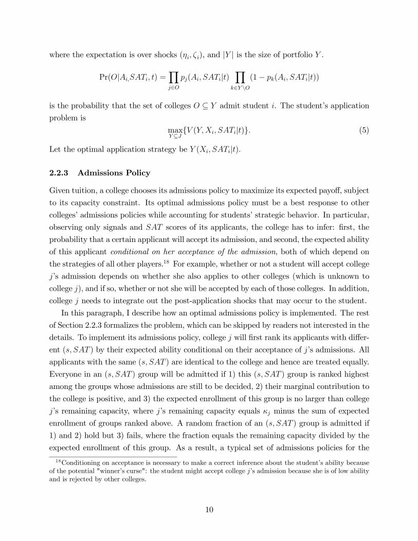
equilibrium pro�les AE(�) in the following subgame, college j�s problem is

maxt0j�0

fE��jjAE(t0j; t�j)

�g: (10)

Independent of its preference on tuition, each college considers the strategic role of its

tuition in the subsequent AE(t0j; t�j). On the one hand, low tuition makes the college more

attractive to students and more competitive in the market. On the other hand, high tuition

serves as a screening tool and leads to a better pool of applicants if high-ability students are

less sensitive to tuition than low-ability students.23 Together with the monetary incentives

of tuition revenue, such trade-o¤s determine the college�s optimal tuition level.

2.4 Subgame Perfect Nash Equilibrium

De�nition 2 A subgame perfect Nash equilibrium for the college market is

(t�; d(�j�); Y (�j�); e(�j�)) such that:(a) For every t, (d(�jt); Y (�jt); e(�jt)) constitutes an AE(t), according to De�nition 1;(b) For every j, given t��j, t

�j is optimal for college j, i.e., solves problem (10) :

In the appendix, I show the existence of equilibrium for a simpli�ed version of the model

with two colleges. Numerically, I have found equilibrium in the full model throughout my

empirical analyses.

3 Estimation Strategy and Identi�cation

3.1 Estimating the Application-Admission Subgame

First, I �x the tuition pro�le at its equilibrium (data) level and estimate the parameters that

govern the application-admission subgame. To save notation, I suppress the dependence of

endogenous objects on tuition.

The estimation is complicated by potential multiple equilibria in the subgame and the fact

that econometricians do not observe the equilibrium selection rule.24 One way to deal with

this complication is to impose some equilibrium selection rule assumed to have been used

by the players and to consider only the selected equilibrium. However, for models like the

23This is a possible scenario. However, in the estimation, I do not impose any restriction on the relationshipbetween student ability and their sensitivity to prices.24The problem of possible multiple equilibria is a di¢ cult, yet frequent problem in structual equilibrium

models. For example, the model by Epple, Romano and Sieg (2006) also admits multiple equilibria, and theauthors assume unique equilibrium in their estimation and other empirical analyses.

13

one in this paper, there is not a single compelling selection rule (from the econometrician�s

point of view).25 I use a two-step strategy to estimate the application-admission subgame

without having to impose any equilibrium selection rule.

Each application-admission equilibrium is uniquely summarized in the admissions prob-

abilities fpj(A; SAT )g, which provide su¢ cient information for players to make their uniqueoptimal decisions. In the student decision model, fpj(A; SAT )g are taken as given just likeall the other parameters are. Step One treats fpj(A; SAT )g as parameters and estimatesthem along with structural student-side parameters, thereby identifying the equilibrium that

generated the data.26 Step two imposes colleges�optimal admissions policies, which yield a

new set of admissions probabilities. Under the true college-side parameters, these probabil-

ities should match the equilibrium admissions probabilities estimated in the �rst step.

3.1.1 Step One: Estimate Fundamental Student-Side Parameters and Equilib-rium Admissions Probabilities

I implement the �rst step via simulated maximum likelihood estimation (SMLE): together

with estimates of the fundamental student-side parameters�b�0�, the estimated equilibrium

admissions probabilities bp should maximize the probability of the observed outcomes ofapplications, admissions, �nancial aid and enrollment, conditional on observable student

characteristics, i.e., f(Yi;Oi; fi; dijSATi; Bi)gi. �0 is composed of 1) preference parameters�0u = [fuj(T )g;

��j]0, 2) application cost parameters �0C = [C(1); :::; C(J)]0, 3) �nancial

aid parameters �0f , 4) the standard deviation of the shock to the outside option �0� = ��

and 5) the parameters involved in the distribution of types �0T .

Suppose student i is of type T . Her contribution to the likelihood, denoted by

LiT (�0u;�0C ;�0f ;�0� ; p), is composed of the following parts:

LYiT (�0u;�0C ;�0f ;�0� ; p)� the contribution of applications Yi;LOiT (p)� the contribution of admissions OijYi;LfiT (�0f )� the contribution of �nancial aid fijOi, andLdiT (�0u;�0f ;�0�)� the contribution of enrollment dij(Oi; fi):25See, for example, Mailath, Okuno-Fujiwara and Postlewaite (1993), who question the logical foundations

and performances of many popular equilibrium selection rules.26Given admissions probabilities, students�application strategies are independent, which yields a unique

equilibrium in the student-side problem. This may not hold if students directly value the quality of theirpeers. With peer e¤ects, multiple equilibria may coexist in both the student-side and the college-side problem,inducing substantial complications into the model. The existence of peer e¤ects has been controversial inthe higher-education literature. (See, for example, Sacerdote (2001), Zimmerman (2003), Arcidiacono andNicholson (2005) and Dale and Krueger (1998)). In this paper, I focus on the interactions between collegesand students and the competition among colleges, leaving the inclusion of interactions among students forfuture research.

14

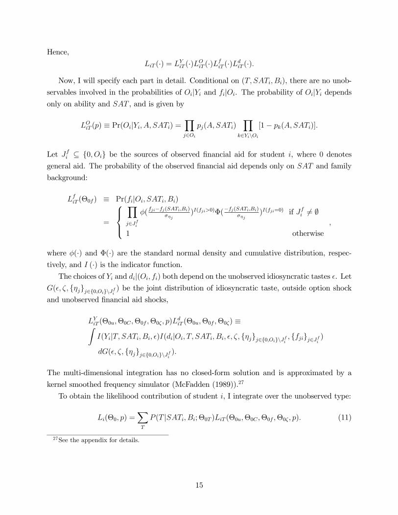
Hence,

LiT (�) = LYiT (�)LOiT (�)LfiT (�)LdiT (�):

Now, I will specify each part in detail. Conditional on (T; SATi; Bi), there are no unob-

servables involved in the probabilities of OijYi and fijOi. The probability of OijYi dependsonly on ability and SAT , and is given by

LOiT (p) � Pr(OijYi; A; SATi) =Yj2Oi

pj(A; SATi)Y

k2YinOi

[1� pk(A; SATi)]:

Let Jfi � f0; Oig be the sources of observed �nancial aid for student i, where 0 denotesgeneral aid. The probability of the observed �nancial aid depends only on SAT and family

background:

LfiT (�0f ) � Pr(fijOi; SATi; Bi)

=

8><>:Yj2Jfi

�(fji�fj(SATi;Bi)

��j)I(fji>0)�(

�fj(SATi;Bi)��j

)I(fji=0) if Jfi 6= ;

1 otherwise;

where �(�) and �(�) are the standard normal density and cumulative distribution, respec-tively, and I (�) is the indicator function.The choices of Yi and dij(Oi; fi) both depend on the unobserved idiosyncratic tastes �. Let

G(�; �; f�jgj2f0;OignJfi ) be the joint distribution of idiosyncratic taste, outside option shockand unobserved �nancial aid shocks,

LYiT (�0u;�0C ;�0f ;�0� ; p)LdiT (�0u;�0f ;�0�) �Z

I(YijT; SATi; Bi; �)I(dijOi; T; SATi; Bi; �; �; f�jgj2f0;OignJfi ; ffjigj2Jfi )

dG(�; �; f�jgj2f0;OignJfi ):

The multi-dimensional integration has no closed-form solution and is approximated by a

kernel smoothed frequency simulator (McFadden (1989)).27

To obtain the likelihood contribution of student i, I integrate over the unobserved type:

Li(�0; p) =XT

P (T jSATi; Bi; �0T )LiT (�0u;�0C ;�0f ;�0� ; p): (11)

27See the appendix for details.

15

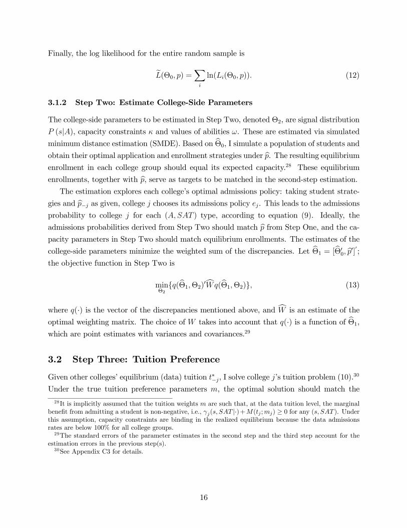
Finally, the log likelihood for the entire random sample is

eL(�0; p) =Xi

ln(Li(�0; p)): (12)

3.1.2 Step Two: Estimate College-Side Parameters

The college-side parameters to be estimated in Step Two, denoted �2, are signal distribution

P (sjA), capacity constraints � and values of abilities !. These are estimated via simulatedminimum distance estimation (SMDE). Based on b�0, I simulate a population of students andobtain their optimal application and enrollment strategies under bp. The resulting equilibriumenrollment in each college group should equal its expected capacity.28 These equilibrium

enrollments, together with bp, serve as targets to be matched in the second-step estimation.The estimation explores each college�s optimal admissions policy: taking student strate-

gies and bp�j as given, college j chooses its admissions policy ej. This leads to the admissionsprobability to college j for each (A; SAT ) type, according to equation (9). Ideally, the

admissions probabilities derived from Step Two should match bp from Step One, and the ca-

pacity parameters in Step Two should match equilibrium enrollments. The estimates of the

college-side parameters minimize the weighted sum of the discrepancies. Let b�1 = [b�00; bp0]0;the objective function in Step Two is

min�2fq(b�1;�2)0cWq(b�1;�2)g; (13)

where q(�) is the vector of the discrepancies mentioned above, and cW is an estimate of the

optimal weighting matrix. The choice of W takes into account that q(�) is a function of b�1,which are point estimates with variances and covariances.29

3.2 Step Three: Tuition Preference

Given other colleges�equilibrium (data) tuition t��j, I solve college j�s tuition problem (10).30

Under the true tuition preference parameters m, the optimal solution should match the

28It is implicitly assumed that the tuition weights m are such that, at the data tuition level, the marginalbene�t from admitting a student is non-negative, i.e., j(s; SAT j�)+M(tj ;mj) � 0 for any (s; SAT ). Underthis assumption, capacity constraints are binding in the realized equilibrium because the data admissionsrates are below 100% for all college groups.29The standard errors of the parameter estimates in the second step and the third step account for the

estimation errors in the previous step(s).30See Appendix C3 for details.

16

tuition data.31 The objective in Step Three is

minmf(t� � t(b�;m))0(t� � t(b�;m))g;

where t� is the data tuition pro�le, t(�) consists of each college�s optimal tuition, and b� �[b�0; b�2] is the vector of fundamental parameter estimates from the previous two steps. I

obtain the variance-covariance of bm using the Delta method, which exploits the variance-

covariance structure of b�:3.3 Identi�cation

Given the policies on tuition, admissions and �nancial aid, students with the same observable

characteristics may make di¤erent application decisions due to their unobserved types and

idiosyncratic tastes. With the latter assumed to be normal, the student-side model can be

viewed as a �nite mixture of multinomial probits. In the appendix, I prove formally the

identi�cation of a mixed probit model with two types, which shares the same logic for the

identi�cation in the more general case of mixed multinomial probits with multiple types.32

In this subsection, I provide a more intuitive discussion about the identi�cation of student

types. Discussions about the identi�cation of some speci�c key parameters will be provided

along with the estimation results. Interested readers can also �nd more formal and detailed

discussions in the appendix.

As is true in most structural models, functional form assumptions and exclusion restric-

tions facilitate the identi�cation. However, the most important source of identi�cation is the

dynamics of the model, which help to identify student types through realizations of admis-

sions and �nancial aid as well as through student application and enrollment decisions. For

example, someone with a strong preference to attend college but low ability will diversify her

risks by sending out more applications, but may be rejected by most of the college groups

she applies to. Besides the sizes of application portfolios, the contents of these portfolios also

inform us about types. In the model, a student�s preferences for di¤erent colleges are corre-

lated via her type-speci�c preference parameters. Consider students with the same SAT and

31Given that there is only a single college market, there are only four tuition observations on which to basethe estimation of the colleges�objective functions. Therefore, pursing a conventional estimation approachis not sensible. Instead, I treat the four nonlinear best response functions as exact, which implies that theeconometrician observes all factors involved in a college�s tuition decision, and saturate the model. Thisapproach also enables me to recover the tuition preference parameters without solving the full equilibriumof the model. As is shown below, the �t to the tuition data is quite good, although there is no statisticalcriterion that can be applied.32The proof builds on Meijer and Ypma (2008), who show the identi�cation for a mixture of two continuous

univariate distributions that are normal.

17

family background, hence the same expected net tuition and ability. Without heterogeneity

along the Z dimension of student type, i.e., the dimension that captures students�preferences

for public relative to private colleges, these students di¤er only in their i.i.d. idiosyncratic

tastes. As a result, there should not be any systematic di¤erence between their application

portfolios. However, in the data when these students send out multiple applications, they

are more likely to concentrate either on public colleges or on private colleges, rather than

applying to a mixture of both. The patterns of such concentration, therefore, inform us

about the distribution of Z and its e¤ects on students�preferences.

4 Data

4.1 NLSY Data and Sample Selection

In NLSY97, a college choice series was administered in years 2003-2005 to respondents from

the 1983 and 1984 birth cohorts who had completed either the 12th grade or a GED at

the time of interview. Respondents provided information about each college to which they

applied, including name and location; any general �nancial aid they may have received;

whether each college to which they applied had accepted them for admission, along with

�nancial aid o¤ered. Information was asked about each application cycle.33 In every survey

year, the respondents also reported on the college(s), if any, they attended during the previous

year. Other available information relevant to this paper includes SAT=ACT score and

�nancial-aid-relevant family information (family income, family assets, race and number of

siblings in college at the time of application).

The sample I use is from the 2303 students within the representative random sample who

were eligible for the college choice survey in at least one of the years 2003-2005. To focus

on �rst-time college application behavior, I de�ne applicants as students whose �rst-time

college application occurred no later than 12 months after they became eligible. Under this

de�nition, 1756 students are either applicants or non-applicants.34 I exclude applications

for early admission. I also drop observations where some critical information, such as the

identity of the college applied to, is missing. The �nal sample size is 1646.

33An application cycle includes applications submitted for the same start date, such as fall 2004.34I exclude students who were already in college before their �rst reported applications. If a student is

observed in more than one cycle, I use only her/his �rst-time application/non-application information.

18

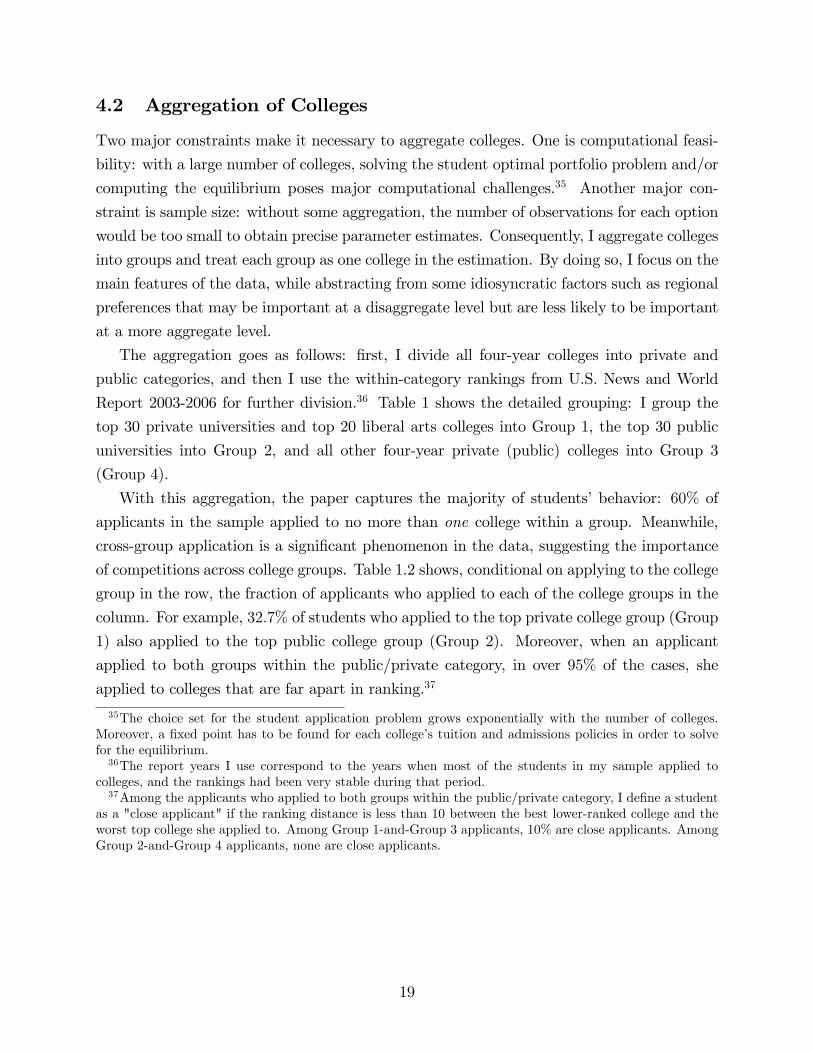
4.2 Aggregation of Colleges

Two major constraints make it necessary to aggregate colleges. One is computational feasi-

bility: with a large number of colleges, solving the student optimal portfolio problem and/or

computing the equilibrium poses major computational challenges.35 Another major con-

straint is sample size: without some aggregation, the number of observations for each option

would be too small to obtain precise parameter estimates. Consequently, I aggregate colleges

into groups and treat each group as one college in the estimation. By doing so, I focus on the

main features of the data, while abstracting from some idiosyncratic factors such as regional

preferences that may be important at a disaggregate level but are less likely to be important

at a more aggregate level.

The aggregation goes as follows: �rst, I divide all four-year colleges into private and

public categories, and then I use the within-category rankings from U.S. News and World

Report 2003-2006 for further division.36 Table 1 shows the detailed grouping: I group the

top 30 private universities and top 20 liberal arts colleges into Group 1, the top 30 public

universities into Group 2, and all other four-year private (public) colleges into Group 3

(Group 4).

With this aggregation, the paper captures the majority of students�behavior: 60% of

applicants in the sample applied to no more than one college within a group. Meanwhile,

cross-group application is a signi�cant phenomenon in the data, suggesting the importance

of competitions across college groups. Table 1.2 shows, conditional on applying to the college

group in the row, the fraction of applicants who applied to each of the college groups in the

column. For example, 32:7% of students who applied to the top private college group (Group

1) also applied to the top public college group (Group 2). Moreover, when an applicant

applied to both groups within the public/private category, in over 95% of the cases, she

applied to colleges that are far apart in ranking.37

35The choice set for the student application problem grows exponentially with the number of colleges.Moreover, a �xed point has to be found for each college�s tuition and admissions policies in order to solvefor the equilibrium.36The report years I use correspond to the years when most of the students in my sample applied to

colleges, and the rankings had been very stable during that period.37Among the applicants who applied to both groups within the public/private category, I de�ne a student

as a "close applicant" if the ranking distance is less than 10 between the best lower-ranked college and theworst top college she applied to. Among Group 1-and-Group 3 applicants, 10% are close applicants. AmongGroup 2-and-Group 4 applicants, none are close applicants.

19

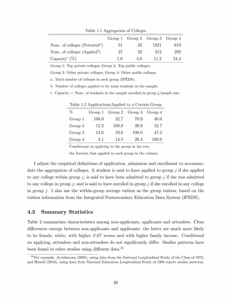
Table 1.1 Aggregation of Colleges

Group 1 Group 2 Group 3 Group 4

Num. of colleges (Potentiala) 51 32 1921 619

Num. of colleges (Appliedb) 37 32 312 292

Capacityc (%) 1:0 4:6 11:2 24:4

Group 1: Top private colleges; Group 2: Top public colleges;

Group 3: Other private colleges; Group 4: Other public colleges.

a. Total number of colleges in each group (IPEDS).

b. Number of colleges applied to by some students in the sample.

c. Capacity = Num. of students in the sample enrolled in group j/sample size.

Table 1.2 ApplicationsjApplied to a Certain Group

% Group 1 Group 2 Group 3 Group 4

Group 1 100:0 32:7 70:9 40:0

Group 2 12:2 100:0 39:9 52:7

Group 3 13:0 19:6 100:0 47:2

Group 4 4:1 14:5 26:4 100:0

Conditional on applying to the group in the row,

the fraction that applied to each group in the column.

I adjust the empirical de�nitions of application, admission and enrollment to accommo-

date the aggregation of colleges. A student is said to have applied to group j if she applied

to any college within group j; is said to have been admitted to group j if she was admitted

to any college in group j; and is said to have enrolled in group j if she enrolled in any college

in group j. I also use the within-group average tuition as the group tuition, based on the

tuition information from the Integrated Postsecondary Education Data System (IPEDS).

4.3 Summary Statistics

Table 2 summarizes characteristics among non-applicants, applicants and attendees. Clear

di¤erences emerge between non-applicants and applicants: the latter are much more likely

to be female, white, with higher SAT scores and with higher family income. Conditional

on applying, attendees and non-attendees do not signi�cantly di¤er. Similar patterns have

been found in other studies using di¤erent data.38

38For example, Arcidiacono (2005), using data from the National Longitudinal Study of the Class of 1972,and Howell (2010), using data from National Education Longitudinal Study of 1988 report similar patterns.

20

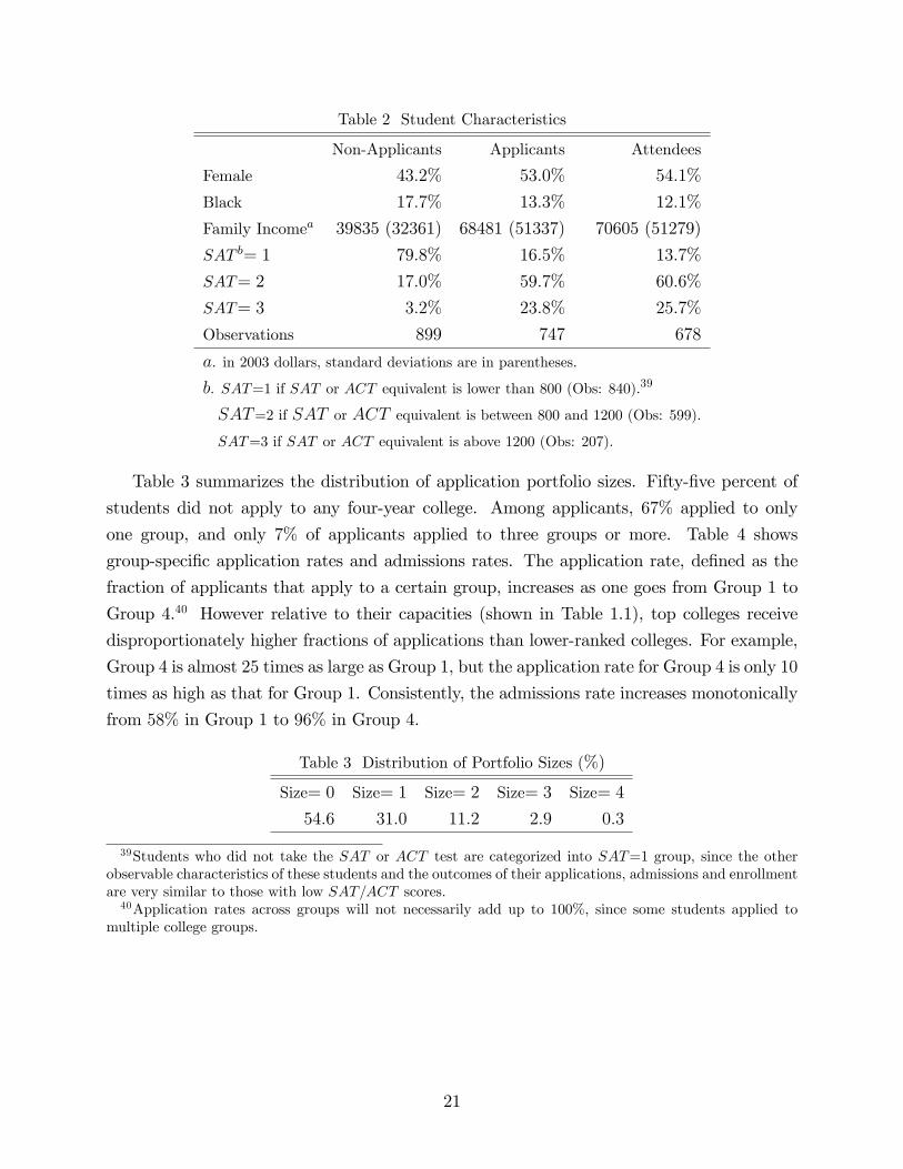
Table 2 Student Characteristics

Non-Applicants Applicants Attendees

Female 43:2% 53:0% 54:1%

Black 17:7% 13:3% 12:1%

Family Incomea 39835 (32361) 68481 (51337) 70605 (51279)

SAT b= 1 79:8% 16:5% 13:7%

SAT= 2 17:0% 59:7% 60:6%

SAT= 3 3:2% 23:8% 25:7%

Observations 899 747 678

a. in 2003 dollars, standard deviations are in parentheses.

b. SAT=1 if SAT or ACT equivalent is lower than 800 (Obs: 840).39

SAT=2 if SAT or ACT equivalent is between 800 and 1200 (Obs: 599).

SAT=3 if SAT or ACT equivalent is above 1200 (Obs: 207).

Table 3 summarizes the distribution of application portfolio sizes. Fifty-�ve percent of

students did not apply to any four-year college. Among applicants, 67% applied to only

one group, and only 7% of applicants applied to three groups or more. Table 4 shows

group-speci�c application rates and admissions rates. The application rate, de�ned as the

fraction of applicants that apply to a certain group, increases as one goes from Group 1 to

Group 4.40 However relative to their capacities (shown in Table 1.1), top colleges receive

disproportionately higher fractions of applications than lower-ranked colleges. For example,

Group 4 is almost 25 times as large as Group 1, but the application rate for Group 4 is only 10

times as high as that for Group 1. Consistently, the admissions rate increases monotonically

from 58% in Group 1 to 96% in Group 4.

Table 3 Distribution of Portfolio Sizes (%)

Size= 0 Size= 1 Size= 2 Size= 3 Size= 4

54:6 31:0 11:2 2:9 0:3

39Students who did not take the SAT or ACT test are categorized into SAT=1 group, since the otherobservable characteristics of these students and the outcomes of their applications, admissions and enrollmentare very similar to those with low SAT=ACT scores.40Application rates across groups will not necessarily add up to 100%; since some students applied to

multiple college groups.

21

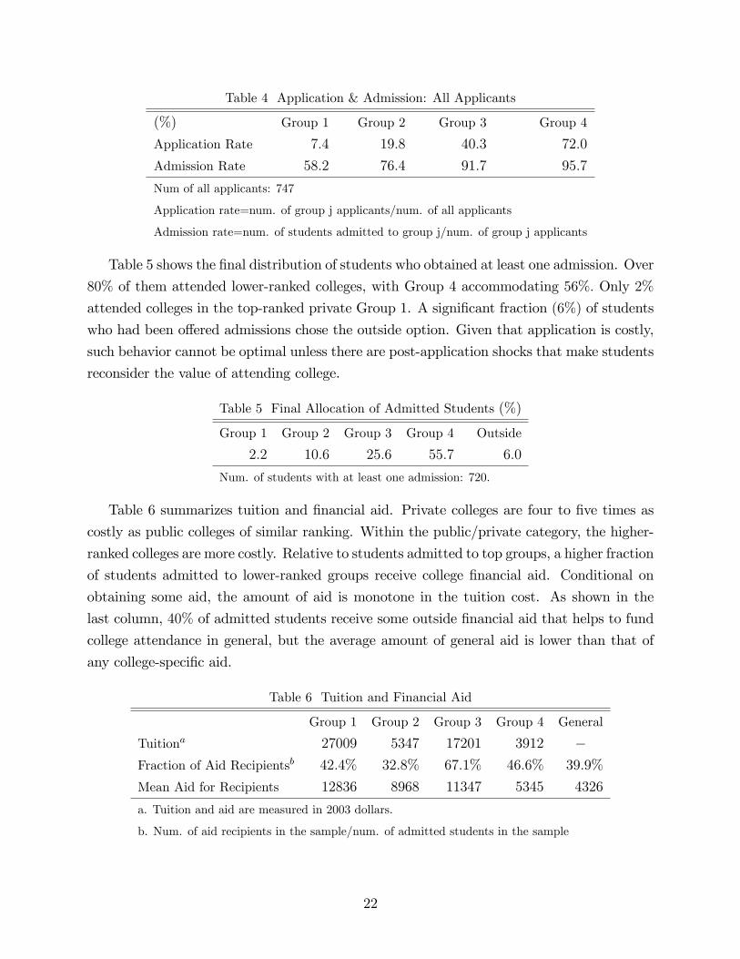
Table 4 Application & Admission: All Applicants

(%) Group 1 Group 2 Group 3 Group 4

Application Rate 7:4 19:8 40:3 72:0

Admission Rate 58:2 76:4 91:7 95:7

Num of all applicants: 747

Application rate=num. of group j applicants/num. of all applicants

Admission rate=num. of students admitted to group j/num. of group j applicants

Table 5 shows the �nal distribution of students who obtained at least one admission. Over

80% of them attended lower-ranked colleges, with Group 4 accommodating 56%: Only 2%

attended colleges in the top-ranked private Group 1. A signi�cant fraction (6%) of students

who had been o¤ered admissions chose the outside option. Given that application is costly,

such behavior cannot be optimal unless there are post-application shocks that make students

reconsider the value of attending college.

Table 5 Final Allocation of Admitted Students (%)

Group 1 Group 2 Group 3 Group 4 Outside

2:2 10:6 25:6 55:7 6:0

Num. of students with at least one admission: 720.

Table 6 summarizes tuition and �nancial aid. Private colleges are four to �ve times as

costly as public colleges of similar ranking. Within the public/private category, the higher-

ranked colleges are more costly. Relative to students admitted to top groups, a higher fraction

of students admitted to lower-ranked groups receive college �nancial aid. Conditional on

obtaining some aid, the amount of aid is monotone in the tuition cost. As shown in the

last column, 40% of admitted students receive some outside �nancial aid that helps to fund

college attendance in general, but the average amount of general aid is lower than that of

any college-speci�c aid.

Table 6 Tuition and Financial Aid

Group 1 Group 2 Group 3 Group 4 General

Tuitiona 27009 5347 17201 3912 �Fraction of Aid Recipientsb 42:4% 32:8% 67:1% 46:6% 39:9%

Mean Aid for Recipients 12836 8968 11347 5345 4326

a. Tuition and aid are measured in 2003 dollars.

b. Num. of aid recipients in the sample/num. of admitted students in the sample

22

5 Empirical Results

This section presents �rst the estimates of some key structural parameters and then the

model �t. More detailed results are in Appendix F2.

5.1 Parameter Estimates

5.1.1 Student Preference

Table 7 Preference Parameter Estimates

($1; 000) Group 1 Group 2 Group 3 Group 4

uj(A = 1; Z = 1) �233:9 (79:8) �287:0 (18:9) �217:0 (8:1) �120:0 (4:5)uj(A = 2; Z = 1) �222:4 (43:6) �97:7 (9:3) �20:9 (3:2) 81:5 (1:1)

uj(A = 3; Z = 1) �57:5 (3:5) 59:7 (6:4) �52:0 (6:1) 11:0 (4:6)

uj(A = 1; Z = 2) �73:9 �309:8 �61:3 �244:7uj(A = 2; Z = 2) �62:4 �120:4 134:8 �43:3uj(A = 3; Z = 2) 124:2 �6:9 37:0 �104:9 j(A 2 f1; 2g) 160:0 (40:9) �22:8 (10:1) 155:7 (4:2) �124:8 (6:8) j(A = 3) 181:7 (26:7) �66:6 (7:5) 89:0 (9:6) �115:9 (21:1)��j 115:0 (1:2) 91:6 (3:8) 77:9 (1:9) 43:6 (1:5)

uj(A;Z = 2) =uj(A;Z = 1)+ j(A), with the restriction that j(1) = j(2):

The restriction cannot be rejected at 10% signi�cance level.

There is signi�cant heterogeneity in students�preferences for colleges, both across types

and within each type. Rows 1 to 3 of Table 7 show the mean values (in $1; 000) attached

to colleges by type Z = 1 students with A = 1 to A = 3, respectively. Rows 4 to 6 show

those values for type Z = 2 students. j(A)�s shown in the next two rows are the additional

values attached to each college group by Z = 2 type relative to Z = 1 type, conditional on

ability. That is, uj(A;Z = 2) = uj(A;Z = 1)+ j(A).

For an average student of the lowest ability (A = 1); attending college is a much worse

option than her outside option. This explains why the majority of (low family income, low

SAT ) students, who are most likely to be of low ability, do not apply to any college in the

data. Due to their low family income, these students would obtain very generous �nancial

aid if they were admitted to any college. Moreover, from an individual student�s point of

view, there is a nontrivial probability that such a student would be admitted, at least, to

the lower-ranked colleges. Given the apparent "unclaimed" bene�ts for these students, their

decisions not to apply inform us that their valuations of colleges must be low.41

41Another potential, but probably minor reason for non-application among these students is borrowingconstraint. For example, Cameron and Heckman (1998) and Keane and Wolpin (2001), �nd that borrowing

23

For students of the two higher ability levels, their valuations of colleges are not universally

monotone in ability: on average, A = 3 students value top colleges more and lower-ranked

colleges less than A = 2 students do. Since these preference parameters re�ect the expected

bene�ts, net of e¤ort costs, of attending colleges, such non-monotone patterns are not com-

pletely surprising. For example, it is reasonable to believe that the e¤ort costs required in

top colleges are higher than those required in lower-ranked colleges, and that these costs

decrease with student ability. Considering the e¤ort costs and the probabilities of success in

di¤erent colleges, a mediocre student might be better o¤ attending a lower-ranked college.

Holding ability constant, Z = 2 type value private colleges more and public colleges less

than Z = 1 type. Private colleges and public colleges have di¤erent features that may �t

some students better than others. For example, private colleges are usually smaller than

public colleges, which may be an advantage for some students but a disadvantage for others.

By introducing types, the model explains the systematic di¤erences in the behaviors

among students with similar observable characteristics. The residual non-systematic di¤er-

ences in student choices are accounted for by their idiosyncratic preferences, where there are

signi�cant dispersions (��j).42 In sum, not only do students attach di¤erent values to the

same college, but they also rank colleges di¤erently. For example, attending an elite college

is not optimal for all students.43 Instead, each option (including the outside option) o¤ered

in the college market best caters to some groups of students.

5.1.2 Application Costs

As shown in Table 8, the cost for the �rst application is about $6; 400, but as the number

of applications increases, the marginal cost rapidly decreases, suggesting the existence of

some economies of scale. Put into context, the application cost is about 6% of the value

of attending college net of tuition for the median applicant, and 5% for the median college

attendee.

Table 8 Application Costs

($1; 000) n = 1 n = 2 n = 3 n = 4

C(n) 6:4 (0:3) 7:9 (0:2) 8:3 (0:2) 8:5 (0:2)

C(n)� C(n� 1) 6:4 1:5 0:4 0:2

constraints have a negligible impact on college attendance, based on which I assume no borrowing constraint.42For example, although Group 1 colleges are worth only $124; 188 for an average student of (A = 3; Z = 2)

type, this value becomes $271; 618 at the 90th percentile. Table F2.1 in the appendix illustrates the im-portance of within-type taste dispersion by showing the mean evaluations of colleges among all students,applicants and attendees, from a simulated example.43This is consistent with �ndings from some other studies, for example, Dale and Krueger (2002).

24

In interpreting these costs, on the one hand, one must remember that they incorporate

all factors that make application costly, i.e., all student-side barriers to applying for colleges

other than their ability and preferences. On the other hand, student ability and preferences

are far more important in explaining the application patterns found in the data. As an

example, in the student decision model, if one �xes all the other parameters, including the

marginal application costs C(n) � C(n � 1) for n > 1, and reduces the cost for the �rst

application to $1; 500; the fraction of non-applicants remains at 51%, as compared to 55%

in the data and in the baseline model. For many students, application costs are irrelevant to

their decisions. For example, average low-ability students, who derive negative utilities from

colleges, will not apply even if application is costless. However, idiosyncratic student tastes

place some students at the margin of applying and not applying, as is true in the data,

where observationally equivalent students may have very di¤erent application behaviors.

The estimates of application costs adjust such that the "right" fraction of marginal students

decide to apply.

5.1.3 Ability Measures

Based on the ability distribution parameter estimates, each row of Table 9.1 shows the

distribution of SAT scores given ability. Ability-1 students are most likely to score low in

SAT , and rarely score high in SAT: Based on SAT; it is relatively easier to distinguish

low-ability students from the others. However, SAT is less useful in distinguishing medium-

ability and high-ability types. For example, most students of both types obtain medium

SAT scores.

Table 9.1 SAT and Ability: Simulation

P (SAT= 1jA) P (SAT= 2jA) P (SAT= 3jA)A = 1 0:79 0:18 0:03

A = 2 0:16 0:63 0:21

A = 3 0:04 0:55 0:41

Table 9.2 reports parameter estimates for the distribution of signals conditional on ability.

Signals, such as student essays, can e¤ectively distinguish the highest ability students from

the others: the former are much more likely to send the highest signal, and almost never

send out the lowest signal. Ability-2 students are most likely to send a medium signal, and

they distinguish themselves from Ability-1 students primarily by their reduced probability of

sending out the lowest signal. However, their chance of obtaining the highest signal is almost

the same as Ability-1 students. As a result, it is hard to distinguish the two lower-ability

types based on their signals.

25

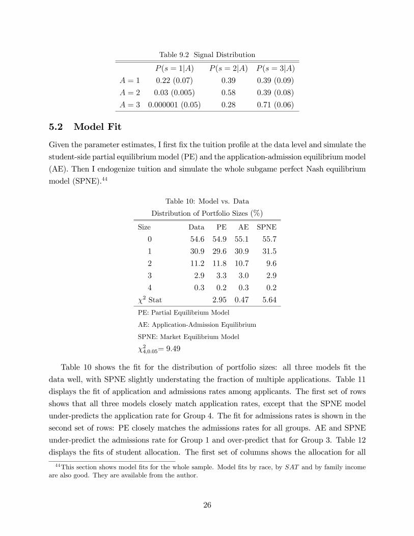
Table 9.2 Signal Distribution

P (s = 1jA) P (s = 2jA) P (s = 3jA)A = 1 0:22 (0:07) 0:39 0:39 (0:09)

A = 2 0:03 (0:005) 0:58 0:39 (0:08)

A = 3 0:000001 (0:05) 0:28 0:71 (0:06)

5.2 Model Fit

Given the parameter estimates, I �rst �x the tuition pro�le at the data level and simulate the

student-side partial equilibriummodel (PE) and the application-admission equilibriummodel

(AE). Then I endogenize tuition and simulate the whole subgame perfect Nash equilibrium

model (SPNE).44

Table 10: Model vs. Data

Distribution of Portfolio Sizes (%)

Size Data PE AE SPNE

0 54:6 54:9 55:1 55:7

1 30:9 29:6 30:9 31:5

2 11:2 11:8 10:7 9:6

3 2:9 3:3 3:0 2:9

4 0:3 0:2 0:3 0:2

�2 Stat 2:95 0:47 5:64

PE: Partial Equilibrium Model

AE: Application-Admission Equilibrium

SPNE: Market Equilibrium Model

�24;0:05= 9:49

Table 10 shows the �t for the distribution of portfolio sizes: all three models �t the

data well, with SPNE slightly understating the fraction of multiple applications. Table 11

displays the �t of application and admissions rates among applicants. The �rst set of rows

shows that all three models closely match application rates, except that the SPNE model

under-predicts the application rate for Group 4. The �t for admissions rates is shown in the

second set of rows: PE closely matches the admissions rates for all groups. AE and SPNE

under-predict the admissions rate for Group 1 and over-predict that for Group 3. Table 12

displays the �ts of student allocation. The �rst set of columns shows the allocation for all

44This section shows model �ts for the whole sample. Model �ts by race, by SAT and by family incomeare also good. They are available from the author.

26

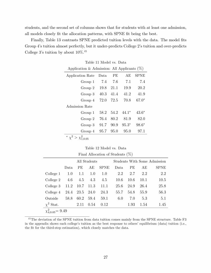
students, and the second set of columns shows that for students with at least one admission,

all models closely �t the allocation patterns, with SPNE �t being the best.

Finally, Table 13 contrasts SPNE predicted tuition levels with the data. The model �ts

Group 4�s tuition almost perfectly, but it under-predicts College 2�s tuition and over-predicts

College 3�s tuition by about 10%.45

Table 11 Model vs. Data

Application & Admission: All Applicants (%)

Application Rate Data PE AE SPNE

Group 1 7:4 7:6 7:1 7:4

Group 2 19:8 21:1 19:9 20:2

Group 3 40:3 41:4 41:2 41:9

Group 4 72:0 72:5 70:8 67:0�

Admission Rate

Group 1 58:2 54:2 44:1� 43:6�

Group 2 76:4 80:2 81:9 82:0

Group 3 91:7 90:9 95:3� 98:6�

Group 4 95:7 95:0 95:0 97:1� �2 > �21;0:05

Table 12 Model vs. Data

Final Allocation of Students (%)

All Students Students With Some Admission

Data PE AE SPNE Data PE AE SPNE

College 1 1:0 1:1 1:0 1:0 2:2 2:7 2:2 2:2

College 2 4:6 4:5 4:3 4:5 10:6 10:6 10:1 10:5

College 3 11:2 10:7 11:3 11:1 25:6 24:9 26:4 25:8

College 4 24:4 23:5 24:0 24:3 55:7 54:8 55:9 56:3

Outside 58:8 60:2 59:4 59:1 6:0 7:0 5:3 5:1

�2 Stat. 2:11 0:54 0:12 1:93 1:54 1:45

�24;0:05= 9:49

45The deviation of the SPNE tuition from data tuition comes mainly from the SPNE structure. Table F3in the appendix shows each college�s tuition as the best response to others�equilibrium (data) tuition (i.e.,the �t for the third-step estimation), which closely matches the data.

27

Table 13: Model vs. Data

Tuition


Data 27009 5347 17201 3912

SPNE 26162 4555 19173 3925

6 Counterfactual Experiments

With the estimated model, which �ts the data reasonably well, I conduct three counterfac-

tual experiments. Comparisons are made between the baseline SPNE and the new SPNE,

simulated using the same set of random draws.46

6.1 Creating More Opportunities

In the �rst counterfactual experiment, I examine to what extent the government can further

expand college access by increasing the supply of colleges. I increase the capacity of the

lower-ranked public colleges (Group 4) by growing magnitudes while keeping the capacities

of other groups �xed.47 The response of college enrollment to the increase in supply is shown

in Figure 1. At the beginning, there is a one-to-one response of college enrollment to the

increase in supply. Then, enrollment reaches a satiation point where there is neither excess

demand nor excess supply of college slots in Group 4 and the equilibrium outcomes remain

the same thereafter. The following tables report the case when Group 4�s supply is at the

satiation point.

Table 14.1 shows changes in tuition. To attract enough students, Group 4 cuts its tuition

from $3; 925 to an almost negligible level of $136. Its private counterpart, Group 3, also

lowers its tuition by about 9%.48 However, the two top groups increase their tuition. To

better understand the di¤erence in colleges�tuition adjustments, we need to jointly consider

their reactions in tuition and admission policies.

46In simulating the baseline model and the counterfactual experiments, I tried a wide range of initialguesses in my search for equilibrium. For each model, I �nd only one equilibrium.47Similar results hold in analogous experiments with Group 3�s capacity. I increase the supply of lower-

ranked colleges because they accommodate most college attendees and are most relevant to the overall accessto college education.48Colleges do not have to �ll their capacities, and they can charge high tuition and leave some slots vacant.

However, under the current situation and the estimated parameter values, it is not optimal for them to doso.

28

0.5

11.

52

2.5

33.

54

4.5

5In

crea

se in

enr

ollm

ent %

0 .5 1 1.5 2 2.5 3 3.5 4 4.5 5Increase in available slots %

Expand Capacity of LowerRanked Colleges

Figure 1: Enrollment & Expansion of Lower-Ranked Groups

Table 14.1 Increasing Supply

Tuition


Base SPNE 26162 4555 19173 3925

New SPNE 27549 6473 17394 136


Admission Rates


Base SPNE 43:6 82:0 98:6 97:1

New SPNE 47:7 99:0 99:1 100:0

Table 14.2 indicates that admissions rates increase in all colleges and reach (almost) 100%

except for Group 1. The major driving forces for the increased admissions rates are likely

to di¤er across college groups. For lower-ranked groups, higher admissions rates and lower

tuition re�ect their e¤orts to enroll enough students. Top groups increase their admissions

rates mainly because they are faced with a better self-selected applicant pool: the increased

tuition in top groups pushes, and the tuition and admissions policies in lower-ranked colleges

pull lower-ability applicants toward lower-ranked groups.

29


Attendance

% Base SPNE New SPNE All Open&Free

All 40:9 43:0 51:1

A = 1 1:9 3:2 14:9

A = 2 94:7 97:7 99:4

A = 3 86:4 90:3 98:6

Table 14.3 shows the allocation e¤ect. The �rst row displays the attendance rate over

all students: regardless of the 100% admissions rate and the dramatically lowered tuition in

Group 4, only 2:1% more students are drawn into colleges. Since the supply of colleges in

Group 4 exceeds demand if its capacity is further increased, this 2:1% increase represents

the upper limit to which the government can increase college attendance by increasing the

supply of Group 4 colleges. To further understand these equilibrium results, I conduct a

partial equilibrium experiment where all colleges are open and free. This is an extreme

situation with unlimited supply of colleges. The attendance rate is reported in the last

column of Table 14.3: only 51%, or 10% more students, would attend colleges under this

condition. Therefore, neither college capacity nor tuition is a major barrier to college access.

The vast majority of students who do not attend colleges under the base SPNE prefer the

outside option over any college option. Among them, most are of low ability. In fact, as

indicated in the last three rows of Table 14.3, only 2% of the lowest-ability students attend

college in the base SPNE, and fewer than 15% of them would attend college even if colleges

were free and open. In contrast, the majority of students of higher ability attend college

in the base SPNE, and almost all of them would attend college if colleges become free and

open. The major limit on college access, therefore, is ability and associated preferences.49

6.2 Ignoring Signals

In some countries, such as China, college admissions are based almost entirely on scores in

a nation-wide test.50 Although such a system may save resources invested in the admissions

process, such as the human resource employed in reading thousands of student essays, it

ignores a valuable source of information about student ability. In the second counterfactual

experiment, I assess the consequences of ignoring signals in the admissions process.

Table 15.1 shows the changes in tuition under the new SPNE. All colleges increase their

tuition, with the top public colleges making the most dramatic increase of 64%: As re�ected49This �nding is in line with earlier research. See, for example, Cameron and Heckman (1998) and Keane

and Wolpin (2001).50Exceptions apply to, for example, students with special talents.

30

by the estimated student preference parameters, higher-ability students have higher prefer-

ences for colleges and hence greater willingness to pay. Knowing this, colleges draw on higher

tuition to screen students when the information on ability provided by signals becomes un-

available. In response to the higher tuition and hence lower net returns from attending

colleges, fewer students apply and applicants apply to fewer colleges, as shown in Table 15.2.

Table 15.1 Ignore Signals

Tuition


Base SPNE 26162 4555 19173 3925

New SPNE 27476 7470 20211 4885


Distribution of Portfolio Sizes


Base SPNE 55:7 31:5 9:6 2:9 0:2

New SPNE 56:0 33:2 8:6 2:2 0:1

Table 15.3 shows the changes in admission rates. With SAT as the single criterion for

admissions, all applicants with the highest SAT are admitted to all colleges. In some colleges,

higher admission rates for higher SAT applicants come at the expense of reduced admissions

for those with lower SAT scores. For example, in the top private colleges, less than 8% of

medium SAT applicants are admitted as compared to 28% in the baseline case. However, the

overall admission rates increase in all colleges as a result of reduced applications. Although

higher tuition levels help to screen students, all colleges experience a drop in their enrollee

ability (Table 15.4). As one might expect, the e¤ect is more obvious in the top groups than

in the lower-ranked groups.


Admission Rates

% All SAT= 1 SAT= 2 SAT= 3

Base New Base New Base New Base New

Group 1 43:6 55:6 N=A� N=A 28:2 7:6 66:7 100:0

Group 2 82:0 91:5 N=A N=A 72:8 86:8 99:4 100:0

Group 3 98:6 100:0 91:7 100:0 100:0 100:0 100:0 100:0

Group 4 97:1 98:2 96:2 88:3 97:7 100:0 97:8 100:0

* Not applicable since application is zero.

31


Fraction of High-Ability Students


Base SPNE 89:9 84:1 11:7 7:2

New SPNE 87:2 82:5 11:5 7:1

Finally, changes in student welfare are reported in Table 15.5. Overall, student welfare

decreases by $1; 325: Although the increase in tuition a¤ects all students negatively, the

changes in admissions policies have di¤erent e¤ects on students with di¤erent abilities. The

highest-ability students lose the most, with a loss of $5; 000: They are the ones who have the

most to gain from signals, through which they can most e¤ectively distinguish themselves

from others. The medium-ability students bene�t from being mixed with the highest-ability

ones, but su¤er from being mixed with the lowest-ability ones. The only winners are the

lowest-ability students: their gain from being mixed with others outweighs the loss from

increased tuition.


Mean Student Welfare

$ Base SPNE New SPNE Change

All 41402 40077 �1325A = 1 677 752 75

A = 2 98630 95907 �2723A = 3 84673 79692 �4981

6.3 Dropping SAT

Although SAT remains one of the most important criteria for admissions to most colleges,

there have been concerns that SAT has been overemphasized. For example, critics have

been blaming SAT as inhibiting the access to higher education for students from low-income

families, who typically have low SAT scores. In response, starting from 1969, a number

of liberal arts colleges have either joined, or have been important in�uences on, the SAT

Optional Movement, which urges dropping SAT in the admissions process.51 In a 2001 speech

to the American Council on Education, Richard Atkinson, the president of the University

of California, also urged dropping the SAT as a college admissions requirement.52 The

51Bowdoin College and Bates College were among the �rst to institute SAT -optional programs in 1969 and1984, respectively. In 2006, 27 of the top 100 liberal arts colleges did not require SAT or ACT: For a completelist of colleges that do not require SAT or ACT in admission, see http://fairtest.org/university/optional.52In response to threats by the University of California to drop the SAT as an admission requirement, the

College Entrance Examination Board announced the restructuring of the SAT , to take e¤ect in March 2005.

32

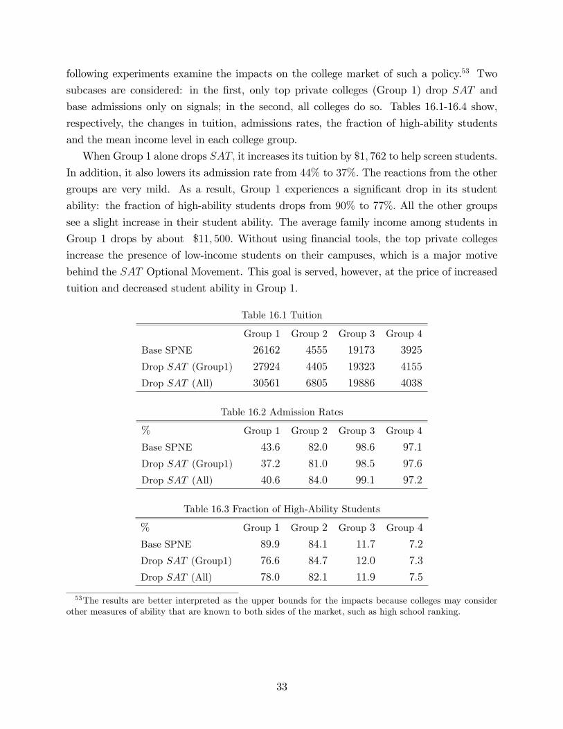
following experiments examine the impacts on the college market of such a policy.53 Two

subcases are considered: in the �rst, only top private colleges (Group 1) drop SAT and

base admissions only on signals; in the second, all colleges do so. Tables 16.1-16.4 show,

respectively, the changes in tuition, admissions rates, the fraction of high-ability students

and the mean income level in each college group.

When Group 1 alone drops SAT; it increases its tuition by $1; 762 to help screen students.

In addition, it also lowers its admission rate from 44% to 37%: The reactions from the other

groups are very mild. As a result, Group 1 experiences a signi�cant drop in its student

ability: the fraction of high-ability students drops from 90% to 77%: All the other groups

see a slight increase in their student ability. The average family income among students in

Group 1 drops by about $11; 500: Without using �nancial tools, the top private colleges

increase the presence of low-income students on their campuses, which is a major motive

behind the SAT Optional Movement. This goal is served, however, at the price of increased

tuition and decreased student ability in Group 1.

Table 16.1 Tuition


Base SPNE 26162 4555 19173 3925

Drop SAT (Group1) 27924 4405 19323 4155

Drop SAT (All) 30561 6805 19886 4038

Table 16.2 Admission Rates


Base SPNE 43:6 82:0 98:6 97:1

Drop SAT (Group1) 37:2 81:0 98:5 97:6

Drop SAT (All) 40:6 84:0 99:1 97:2

Table 16.3 Fraction of High-Ability Students


Base SPNE 89:9 84:1 11:7 7:2

Drop SAT (Group1) 76:6 84:7 12:0 7:3

Drop SAT (All) 78:0 82:1 11:9 7:5

53The results are better interpreted as the upper bounds for the impacts because colleges may considerother measures of ability that are known to both sides of the market, such as high school ranking.

33

Table 16.4 Mean Income

$ Group 1 Group 2 Group 3 Group 4

Base SPNE 93802 90610 65916 64657

Drop SAT (Group 1) 82343 90988 65934 64831

Drop SAT (All) 83205 87560 66206 64587

When all college groups drop SAT; they all increase their tuition to enhance self-selection

among students. The reaction is especially strong in the two top groups: Group 2 increases

its tuition by almost 50%; and Group 1 increases its tuition by more than it does in the �rst

subcase.54 The student bodies in all colleges become more diverse: lower-ranked colleges

obtain more high-ability students, while the top colleges, especially Group 1, obtain more low-

ability and low-family-income students. In the baseline equilibrium, low-SAT students are

discouraged from applying to top colleges because they know their SAT before application

and they know with low SAT; they have (near) zero probability of being admitted. Dropping

SAT , therefore, opens the door to top colleges for high-ability students who happen to

obtain low SAT scores, as desired by the current SAT -optional colleges. However, dropping

SAT also opens the door for low-ability students. These students have a fair chance (39%)

of sending a high signal and a signi�cant number of them have strong preference for top

colleges, especially for the top private group.

7 Conclusion

In this paper, I have developed and structurally estimated an equilibriummodel of the college

market. It provides a �rst step toward a better understanding of the college market by jointly

considering tuition setting, applications, admissions and enrollment. In the model, students

are heterogeneous in their abilities and preferences. They face uncertainty and application

costs when making their application decisions. Colleges, observing only noisy measures

of student ability, compete for more able students via tuition and admissions policies. I

have estimated the structural model via a three-step estimation procedure to cope with the

complications caused by potential multiple equilibria. The empirical results suggest that the

model closely replicates most of the patterns in the data.

My empirical analyses suggest that, �rst, there is substantial heterogeneity in students�

preferences for colleges. As a result, increasing the supply of colleges has very limited e¤ect

on college attendance: neither tuition cost nor college capacity is a major obstacle to college

54This implies that, in Subcase 1, the seeming "lack of reactions" from the other college groups restrictsGroup 1 from taking more dramatic actions.

34

access; a large fraction of students, mainly low-ability students, prefer the outside option

over any college option. Second, there are signi�cant amounts of noise in various types of

ability measures and di¤erent types of measures complement one another. Dropping SAT;

as urged by some critics, indeed increases the fraction of low-income students in top colleges,

but it is accompanied by lower enrollee ability and higher tuition in these colleges.

The methods developed in this paper and the main empirical �ndings are promising for

future research. Building on Epple, Romano and Sieg (2006) and this paper, a model that

endogenizes applications, admissions and �nancial aid would provide a more comprehensive

view of the college market. Given the fast development of computational capacities, this

extension may become feasible in the near future.

Building on Arcidiacono (2005) and this paper, a model that studies the strategic inter-

actions between colleges and students and links them to students�labor market outcomes

would also be an important extension. Such an extension would enrich the current paper

by making explicit the factors underlying student preferences. This will become feasible as

information on students�labor market outcomes becomes available from future surveys of

the NLSY97.

Finally, studying the long-run equilibrium would lead to a better understanding of the

trend of college tuition and attendance. In a long run equilibrium model, one can be more

explicit about why colleges value student ability. For example, higher-ability students are

more likely to do better in the job market, which enhances the college�s prestige and at-

tractiveness to future applicants. Moreover, one can also endogenize college capacities. One

approach to implement this extension is to introduce a cost function for college education,

assuming free entry to the market. Equilibrium of the model would then depend on the form

of the cost function. Estimation of such a model would require additional data on college

expenses and non-tuition revenues, as well as application and admissions data over multiple

years.

References

Arcidiacono, Peter. 2005. "A¢ rmative Action in Higher Education: How Do Admission and

Financial Aid Rules A¤ect Future Earnings?" Econometrica, 73(5): 1477-1524.

Arcidiacono, Peter and Sean Nicholson. 2005. "Peer e¤ects in medical school." Journal of

Public Economics, 89(2-3): 327-350

Avery, Christopher, Andrew Fairbanks and Richard Zeckhauser. 2003. The Early Admissions

Game: Joining the Elite. Cambridge, MA: Harvard University Press.

35

Avery, Christopher, Jonathan Levin. 2010. "Early Admissions at Selective Colleges." Amer-

ican Economic Review, 100(6): 1-34.

Bowen, William and Derek Bok. 1998. The Shape of the River: Long-Term Consequences of

Considering Race in College and University Admissions. Princeton, NJ: Princeton University

Press.

Chade, Hector, Gregory Lewis and Lones Smith. 2011. "Student Portfolios and the College

Admissions Problem." Social Science Research Network Working Paper 135834.

Cameron, Stephen and James Heckman. 1998. �Life Cycle Schooling and Dynamic Selec-

tion Bias: Models and Evidence for Five Cohorts of American Males.�Journal of Political

Economy, 106(2): 262-333.

Dale, Stacy and Alan Krueger. 2002. "Estimating The Payo¤To Attending A More Selective

College: An Application Of Selection On Observables And Unobservables." The Quarterly

Journal of Economics, 117(4): 1491-1527.

Epple, Dennis, Richard Romano and Holger Sieg. 2006. "Admission, Tuition, And Financial

Aid Policies in The Market For Higher Education." Econometrica, 74(4): 885-928.

Howell, Jessica. 2010. "Assessing the Impact of Eliminating A¢ rmative Action in Higher

Education." Journal of Labor Economics, 28(1): 113-166.

Light, Audrey andWayne Strayer. 2002. �From Bakke to Hopwood: Does Race A¤ect College

Attendance and Completion?�The Review of Economics and Statistics, 85: 34-44.

McFadden, Daniel. 1989. �A Method of Simulated Moments for Estimation of Discrete Re-

sponse Models without Numerical Integration.�Econometrica, 57(5): 995-1026.

Kane, Thomas. 1998. �Racial and Ethnic Preferences in College Admissions.�in The Black-

White Test Score Gap, ed. Christopher Jencks and Meredith Phillips, 971-996. Washington

D.C.: Brookings Institution Press.

Mailath, George, Masahiro Okuno-Fujiwara and Andrew Postlewaite. 1993. "On Belief Based

Re�nements in Signaling Games." Journal of Economic Theory, 60: 241-276.

Manski, Charles and DavidWise. 1983. College Choice in America. Cambridge, MA: Harvard

University Press

Meijer, Erik and Jelmer Ypma. 2008. "A Simple Identi�cation Proof for a Mixture of Two

Univariate Normal Distributions." Journal of Classi�cation, 25: 113-123.

36

Moro, Andrea. 2003. �The E¤ect of Statistical Discrimination on Black-White Wage Dif-

ferentials: Estimating a Model with Multiple Equilibria.� International Economic Review,

44(2): 467-500.

Nagypál, Eva. 2004. "Optimal Application Behavior with Incomplete Information." mimeo,

Northwestern University.

Keane, Michael and Kenneth Wolpin. 2001. "The E¤ect of Parental Transfers and Borrowing

Constraints on Educational Attainment." International Economic Review, 42(4): 1051-1103.

Sacerdote, Bruce. 2001. �Peer E¤ects with Random Assignment: Results from Dartmouth

Roommates.�Quarterly Journal of Economics, 116: 681�704.

Zimmerman, David. 2003. �Peer E¤ects in Higher Education: Evidence from a Natural

Experiment.�The Review of Economics and Statistics, 85: 9�23.

APPENDIX:

A. Model Details:A1. College Admission Problem: �j(s; SAT jt; e�j; Y; d) and j(s; SAT jt; e�j; Y; d)All objects de�ned in A1 depend on ft; e�j; Y; dg. To save notation, the dependence is

suppressed. Let Pr(acceptjX;SAT; �; �; j) be the probability that a student with character-istics (X;SAT; �; �) who applies to Group j accepts j�s admission. Let F (X; �; �js; SAT; j)be the distribution of (X; �; �) conditional on (s; SAT ) and application to j. The probability

that an applicant with (s; SAT ) accepts j�s admission is:

�j(s; SAT j�) =ZPr(acceptjX;SAT; �; �; j)dF (X; �; �js; SAT; j).

Let Pr(O�jjA; SAT ) �Yl2Onj

pl(A; SAT )Y

k2Y nO

(1� pk(A; SAT )) be the probability of admis-

sion set O for a student with (A; SAT ), with college j admitting her for sure,

Pr(acceptjX;SAT; �; �; j) =X

O�j�Y (X;SAT )nfjg

Pr(O�jjA; SAT )I(j = d(X;SAT; �; �; O)):

That is, the student will accept j�s admission if j is the best post-application choice for her.

The distribution F (X; �; �js; SAT; j) is given by

dF (X; �; �js; SAT; j) = P (sjA)I(j 2 Y (X;SAT ))dH(X; �; �jSAT )RP (sjA)I(j 2 Y (X;SAT ))dH(X; �; �jSAT ) ;

37

where H(X; �; �jSAT ) is exogenous and equal to the product of type distribution, the dis-tribution of ex-post shocks and the distribution of family backgrounds conditional on SAT .

Finally, the expected ability of applicant (s; SAT ) conditional on acceptance is

j(s; SAT j�) =RA� Pr(acceptjX;SAT; �; �; j)dF (X; �; �js; SAT; j)

�j(s; SAT j�):

A2. Proof of existence in a simpli�ed model.

Assume there are two colleges j 2 f1; 2g and a continuum of students divided into two

ability levels. The utility of the outside option is normalized to 0. The utility of attending

college 1 is u1(A) for all with ability A, and that of attending college 2 is u2(A) + �, where

� is i.i.d. idiosyncratic taste. There are two SAT levels and two signal levels. There is

no ex-post shock. Some notations to be used: for an (A; SAT ) group, let the fraction of

students that do not apply to any college be �0A;SAT , the fraction of those applying to college

j only be �jA;SAT and the fraction applying to both be �12A;SAT . For each (A; SAT ) group,

�A;SAT 2 �, a 3-simplex. For all four (A; SAT ) groups, � 2 � � �4. On the college side,

each college chooses admissions policy ej 2 [0; 1]4, where 4 is the number of (s; SAT ) groupsfaced by the college.

Proposition 1 For any given tuition pro�le t, an application-admission equilibrium exists.

Proof. Step 1: The application-admission model can be decomposed into the followingsub-mappings:

Taking the distribution of applicants, and the admissions policy of the other college as given,

college j�s problem (6) can be viewed as the sub-mapping

Mj : �� [0; 1]4 � [0; 1]4;

for j = 1; 2. Taking college admissions policies as given, the distribution of students is

obtained via the sub-mapping

M3 : [0; 1]4 � [0; 1]4 ! �:

An equilibrium is a �xed point of the mapping:

M : �� [0; 1]4 � [0; 1]4 � �� [0; 1]4 � [0; 1]4

s:t: � 2 M3(e1;e2)

ej 2 Mj(�; ek) j; k 2 f1; 2g; j 6= k:

38

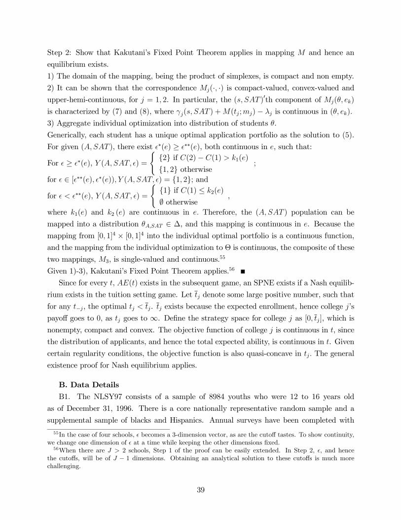
Step 2: Show that Kakutani�s Fixed Point Theorem applies in mapping M and hence an

equilibrium exists.

1) The domain of the mapping, being the product of simplexes, is compact and non empty.

2) It can be shown that the correspondence Mj(�; �) is compact-valued, convex-valued andupper-hemi-continuous, for j = 1; 2. In particular, the (s; SAT )0th component of Mj(�; ek)

is characterized by (7) and (8), where j(s; SAT ) +M(tj;mj)� �j is continuous in (�; ek):

3) Aggregate individual optimization into distribution of students �.

Generically, each student has a unique optimal application portfolio as the solution to (5).

For given (A; SAT ), there exist ��(e) � ��(e), both continuous in e, such that:

For � � ��(e), Y (A; SAT; �) =

(f2g if C(2)� C(1) > k1(e)

f1; 2g otherwise;

for � 2 [��(e); ��(e)); Y (A; SAT; �) = f1; 2g; and

for � < ��(e), Y (A; SAT; �) =

(f1g if C(1) � k2(e)

; otherwise,

where k1(e) and k2 (e) are continuous in e: Therefore, the (A; SAT ) population can be

mapped into a distribution �A;SAT 2 �, and this mapping is continuous in e. Because themapping from [0; 1]4 � [0; 1]4 into the individual optimal portfolio is a continuous function,and the mapping from the individual optimization to � is continuous, the composite of these

two mappings, M3, is single-valued and continuous.55

Given 1)-3), Kakutani�s Fixed Point Theorem applies.56

Since for every t, AE(t) exists in the subsequent game, an SPNE exists if a Nash equilib-

rium exists in the tuition setting game. Let tj denote some large positive number, such that

for any t�j, the optimal tj < tj. tj exists because the expected enrollment, hence college j�s

payo¤ goes to 0; as tj goes to 1. De�ne the strategy space for college j as [0; tj], which isnonempty, compact and convex. The objective function of college j is continuous in t, since

the distribution of applicants, and hence the total expected ability, is continuous in t. Given

certain regularity conditions, the objective function is also quasi-concave in tj: The general

existence proof for Nash equilibrium applies.

B. Data DetailsB1. The NLSY97 consists of a sample of 8984 youths who were 12 to 16 years old

as of December 31, 1996. There is a core nationally representative random sample and a

supplemental sample of blacks and Hispanics. Annual surveys have been completed with

55In the case of four schools, � becomes a 3-dimension vector, as are the cuto¤ tastes. To show continuity,we change one dimension of � at a time while keeping the other dimensions �xed.56When there are J > 2 schools, Step 1 of the proof can be easily extended. In Step 2, �, and hence

the cuto¤s, will be of J � 1 dimensions. Obtaining an analytical solution to these cuto¤s is much morechallenging.

39

most of these respondents since 1997.

B2. Empirical De�nition of Early Admission:

1) Applications were sent earlier than Nov. 30th, for attendance in the next fall semester

and

2) The intended college has early admissions/ early decision/ rolling admissions/ priority

admissions policy,57 and

3) Either a: one application was sent early and led to an admission or

b: some application(s) was (were) sent early but rejected, and other application(s) was

(were) sent later.

B3. Since 1983, U.S. News andWorld Report has been publishing annual rankings of U.S.

colleges and is the most widely quoted of its kind in the U.S.58 Each year, seven indicators

are used to evaluate the academic quality of colleges for the previous academic year.59

C. Details on EstimationC1. Details on SMLE:

(1) Approximate the following integration via a kernel smoothed frequency simulator 60ZI(YijT; SATi; Bi; �)I(dijOi; T; SATi; Bi; �; �; �)dG(�; �; �): (14)

For each student (SATi; Bi), I draw shocks f(�ir; � ir; �ir)gRr=1 from their joint distributionG(�): These shocks are the same across T for the same student i, but are i.i.d. across

students. All shocks are �xed throughout the estimation. Let ujir be the ex-post value of

college j for studentir with (T; SATi; Bi; �ir; � ir; �ir), let vir = maxf0; fujirgj2Oig, let Vir(Y )be the ex-ante value of portfolio Y for this student, and V �

ir = maxY�JfVir(Y )g. (14) is then57The data source for college early admission programs is 1) Christopher et al. (2003), and 2) web

information posted by individual colleges.58The exception is 1984, when the report was interrupted.59These indicators include: assessment by administrators at peer institutions, retention of students, faculty

resources, student selectivity, �nancial resources, alumni giving, and (for national universities and liberalarts colleges) "graduation rate performance", the di¤erence between the proportion of students expected tograduate and the proportion who actually do. The indicators include input measures that re�ect a school�sstudent body, its faculty, and its �nancial resources, along with outcome measures that signal how well theinstitution does its job of educating students.60I describe the situation where I do not observe any information about the student�s �nancial aid. For

students with some �nancial aid information, the observed �nancial aid replaces the random draw of thecorresponding �nancial aid shock.

40

approximated by:

1

R

RXr=1

exp[(Vir(Yi)� V �ir)=� 1]P

Y�J exp[(Vir(Y )� V �ir)=� 1]

exp[(udiir � vir)=� 2]Pj2Oi exp[(ujir � vir)=� 2]

;

where � 1; � 2 are smoothing parameters. When � ! 0, the approximation converges to the

frequency simulator.

(2) Solving the optimal application problem for student (T; SATi; Bi; �ir) :

Vi(Y ) =XO�Y

Pri(O)E(�;�)maxfu0ir;fujirgj2Og � C(jY j):

The Emax function has no closed-form expression and is approximated via simulation. For

each (T; SATi; Bi; �ir), draw M sets of shocks f(�m; �m)gMm=1. For each of the M sets of

(T; SATi; Bi; �ir; �m; �m), calculate maxfu0irm;fujirmgj2Og, where ujirm denotes ujir evalu-

ated at the shock (�m; �m): The Emax is the average of these M maximum values.

C2. Details on the Second-Step SMDE:

(1) Targets to be matched: for each of the Groups 2; 3 and 4, there are 9 admissions

probabilities to be matched fpj (A; SAT )g(A;SAT )2f1;2;3g�f1;2;3g. For Group 1, there are 6admissions probabilities to be matched. Since no one in SAT = 1 group applied to Group

1, fp1 (A; SAT = 1)gA2f1;2;3g are �xed at 0. The other four targets are the equilibrium

enrollments simulated from the �rst step. In all, there are 37 targets to be matched using

college-side parameters: fP (sjA)g; f�jgj, ten of which are free.(2) Optimal Weighting Matrix:

Let �� be the true parameter values. The �rst-step estimates b�1, being MLE, are as-ymptotically distributed as N(0;1). It can be shown that the optimal weighting matrix

for the second-step objective function (13) is W = Q11Q01, where Q1 is the derivative of

q(�) with respect to b�1, evaluated at �b�1;��2�. The estimation of W involves the following

steps:

1) Estimate the variance-covariance matrix b1 : in the case of MLE, this is minus theouter product of the score functions evaluated at b�1. The score functions are obtained vianumerically taking partial derivatives of the likelihood function with respect to each of the

�rst step parameters evaluated at b�1:2) Obtain preliminary estimates e�2 � argmin�2fq(b�1;�2)0fWq(b�1;�2)g, wherefW is any

positive-de�nite matrix. The resulting e�2 is a consistent estimator of ��2:3) Estimate Q1 by numerically taking derivative of q(�) with respect to b�1, evalu-

ated at�b�1; e�2�. In particular, let �m denote a vector with zeros everywhere but the

41

m�th entry, which equals a small number "m. At each�b�1 +�m; e�2�, I simulate the

student decision model and calculate the targets for the second-step estimation. Then

holding student applications �xed, I solve for college optimal admissions and calculate

the distance vector q�b�1 +�m; e�2�. The m�th component of Q1 is approximated by

[q�b�1 +�m; e�2�� q

�b�1; e�2�]="m:C3. Details on the Third-Step: Solving College j�s Tuition Problem

Given b�, t��j and some m, I examine college j�s expected payo¤ at each trial tuition levelt0j and obtain the optimal tuition associated with this m. This procedure requires computing

the series of application-admission equilibria AE��; t��j

�, which can only be achieved through

simulation. To do so, I use an algorithm motivated by the rule of "continuity of equilibria,"

which requires, intuitively, that AE(t0j; t��j) be close to AE(tj; t

��j) when t

0j is close to tj.

Speci�cally, I start from the equilibrium at the data tuition level�t�j ; t

��j�, which is numeri-

cally unique for nontrivial initial beliefs (p >> 0). AE(t�) is found to be unique numerically

in my search for equilibrium starting from 500 di¤erent combinations of nontrivial initial

beliefs. Then, I gradually deviate from t�j , for�t"j ; t

��j�, I start the search for new equilib-

rium, i.e., the �xed point of admissions policies e�:j�t"j ; t

��j��, using, as the initial guess, the

equilibrium e�:j�t0j; t

��j��associated with the most adjacent

�t0j; t

��j�. The resulting series of

AE�:; t��j

�is used to solve college j�s tuition problem.

D. Detailed Functional Forms:D1. Type Distribution:

P (T jSAT;B) = Pr(A = ajSAT;B)P (ZjA) = Pr(A = ajSAT; y)P (ZjA), where y isfamily income, Pr(A = ajSAT; y) is an ordered logistic distribution and P (ZjA) is non-parametric. For a = 1; 2; 3

Pr(A = ajSAT; y) = 1

1 + e�cuta+�1yi+�2I(SATi=2)+�3I(SATi=3)

� 1

1 + e�cuta�1+�1yi+�2I(SATi=2)+�3I(SATi=3)

where cut0 = �1 and cut3 = +1:

D2. College Payo¤ from Tuition Revenue:

M(tj;mj) = mj1tj +mj2t2j

A non-linear preference over tuition is assumed because most colleges are non-pro�t, and

a non-linear preference allows for possibly satiated preference over tuition. For example,

42

state governments (alumni) may have objections to very high tuition levels, and adjust their

funding (donations) to colleges accordingly. A concave preference for tuition can be derived

if high tuition crowds out non-tuition revenues.61 ;62

D3. Financial Aid Functions:

f0(SATi; Bi) = �00 + �01I(racei = black) + �02I(SATi = 2) + �03I(SATi = 3)

+�04yi + �05asseti

f0i = maxff0(SATi; Bi) + �0i; 0g;

where �0i~i:i:d:N(0; �2f0): for j = 1; 2::4

fj(SATi; Bi) =

�10 +�11I(racei = black) + �12I(SATi = 2) + �13I(SATi = 3) + �14yi + �15asseti

+�16I(nsib > 0) + �17I(SATi = 2)I(j 2 public) + �18I(SATi = 3)I(j 2 public)+�19I(j = 2) + �110I(j = 3) + �111I(j = 4)

fji = maxffj(SATi; Bi) + �ji; 0g

where nsib denotes the number of siblings in college at the time of i�s application and

�ji~i:i:d:N(0; �2f1):

E. Identi�cationE1. Type distribution and type-speci�c utilities

In the following, I will prove the identi�cation of a mixed probit model with two types.

The identi�cation of the more general case of mixed multinomial probits with multiple types

would require more complicated algebraic analyses but would nevertheless follow the same

logic.

E1.1 Identi�cation of a mixed probit model with two types

Assume there are two unobserved types of individuals A 2 f1; 2g, and Pr(A = 1) = �.

Let the continuous variable z 2 Z � R be an observed individual characteristics and f (�) bea di¤erentiable function of z. Let y 2 f0; 1g be the observed discrete choice, which relates61In particular, if non-tuition revenue for college j adjusts to tuition level according to �0j��1jtj��2jt2j ;

where �0j is the maximum level of college j�s non-tuition revenue; let the tradeo¤ between ability and total(tuition and non-tuition) revenue be m0j ; then the tuition weight parameters in the model can be derivedas m1j = m0j(1��1j) and m2j = �m0j�2j :62I also tried some other functional forms. For example, a linear preference over tuition is rejected because

it predicts much higher tuition levels than are observed in the data.

43

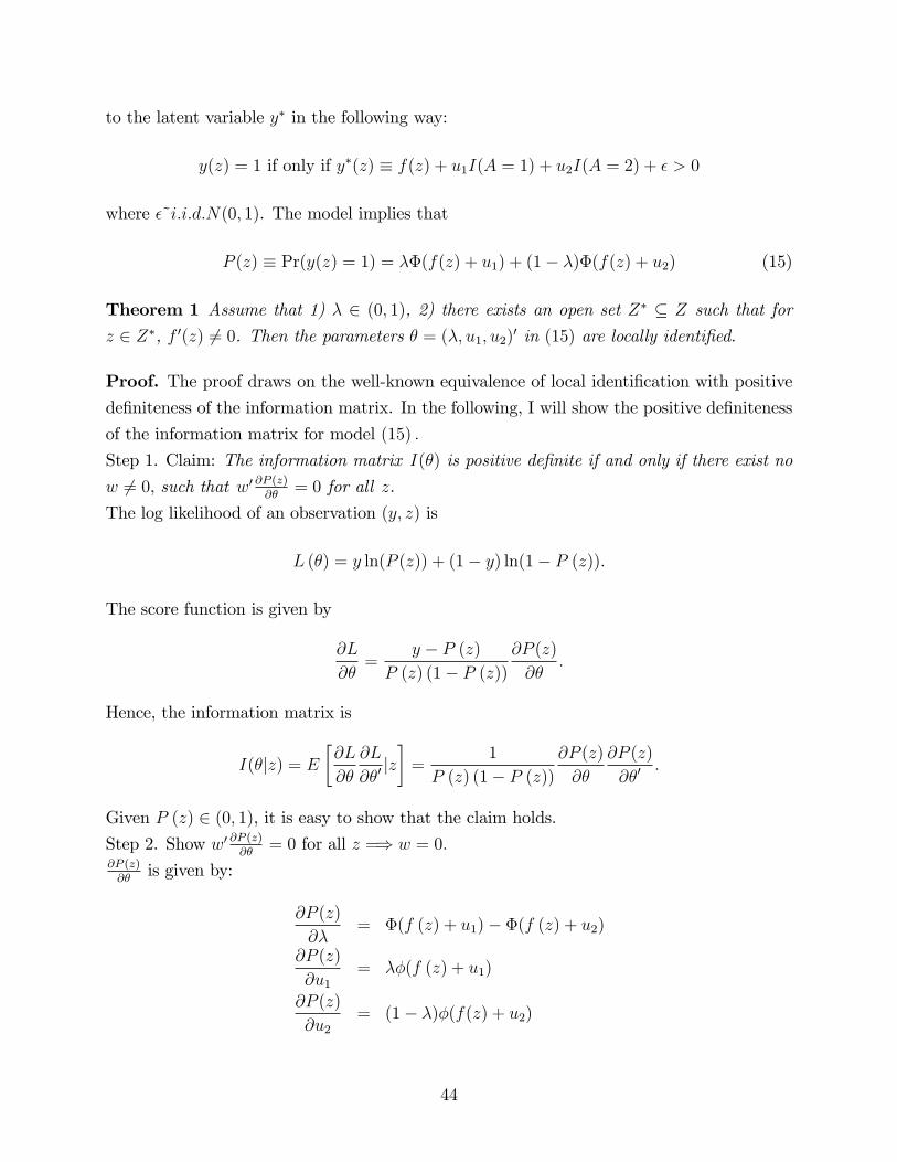
to the latent variable y� in the following way:

y(z) = 1 if only if y�(z) � f(z) + u1I(A = 1) + u2I(A = 2) + � > 0

where �~i:i:d:N(0; 1). The model implies that

P (z) � Pr(y(z) = 1) = ��(f(z) + u1) + (1� �)�(f(z) + u2) (15)

Theorem 1 Assume that 1) � 2 (0; 1), 2) there exists an open set Z� � Z such that for

z 2 Z�, f 0(z) 6= 0. Then the parameters � = (�; u1; u2)0 in (15) are locally identi�ed.

Proof. The proof draws on the well-known equivalence of local identi�cation with positivede�niteness of the information matrix. In the following, I will show the positive de�niteness

of the information matrix for model (15) :

Step 1. Claim: The information matrix I(�) is positive de�nite if and only if there exist no

w 6= 0, such that w0 @P (z)@�

= 0 for all z.

The log likelihood of an observation (y; z) is

L (�) = y ln(P (z)) + (1� y) ln(1� P (z)):

The score function is given by

@L

@�=

y � P (z)

P (z) (1� P (z))

@P (z)

@�:

Hence, the information matrix is

I(�jz) = E

�@L

@�

@L

@�0jz�=

1

P (z) (1� P (z))

@P (z)

@�

@P (z)

@�0:

Given P (z) 2 (0; 1), it is easy to show that the claim holds.

Step 2. Show w0 @P (z)@�

= 0 for all z =) w = 0:@P (z)@�

is given by:

@P (z)

@�= �(f (z) + u1)� �(f (z) + u2)

@P (z)

@u1= ��(f (z) + u1)

@P (z)

@u2= (1� �)�(f(z) + u2)

44

Suppose for some w; w0 @P (z)@�

= 0 for all z :

w1[�(f (z) + u1)� �(f (z) + u2)] + w2��(f (z) + u1) + w3(1� �)�(f(z) + u2) = 0

Take derivative with respect to z evaluated at some z 2 Z�

w1[�(f (z) + u1)� �(f (z) + u2)]f0(z) + w2��

0(f (z) + u1)f0 (z) (16)

+w3(1� �)�0(f(z) + u2)f0 (z) = 0:

De�ne (z) = �(f(z)+u1)�(f(z)+u2)

, divide (16) by �(f (z) + u2) :

w1[ (z)� 1]� w2�(f (z) + u1) (z)� w3(1� �)(f(z) + u2) = 0

(z) [w1 � w2�(f (z) + u1)]� [w1 + w3(1� �)(f(z) + u2)] = 0 (17)

Since (z) is a nontrivial exponential function of z, (17) hold for all z 2 Z� only if both

terms in brackets are zero for each z 2 Z�, i.e.

w1 � w2�(f (z) + u1) = 0 (18)

w1 + w3(1� �)(f(z) + u2) = 0:

Take derivative of (18) again with respect to z, evaluated at z 2 Z� :

w2�f0 (z) = 0

w3(1� �)f 0(z) = 0:

Since � 2 (0; 1) and f 0(z) 6= 0 for some z; w = 0.

E1.2 Relating the proof to the model

In the previous proof, type distribution is assumed to be a single parameter �: In practice,

I assume a logistic distribution of types based on observables. In particular, I assume that

only SAT and family income (a 5-year average) enter the type distribution, i.e., SAT and

family (permanent) income summarize all information that correlates with ability. The

expected �nancial aid net of tuition serves the role of the f (�) function in the previousproof. It depends on SAT and all family-background variables. For example, conditional

on family permanent income, family assets (which serves the role of the z variable in the

previous proof) vary with factors, such as housing prices and stock prices, that are not

45

correlated with ability.63

E2. Other student-side parameters

Given the identi�cation results from the mixture of probits, I now discuss the major

sources for the identi�cation of other student-side parameters. However, readers should be

reminded that all parameters are jointly identi�ed.

E2.1 The probabilities of admissions fpj (A; SAT )gIn the data, we observe the admission rates for students given their SAT and family

income (y), which is generated via the following equation:

Pr (Admssion to jjSAT; y) =XA

Pr(AjSAT; y)pj(A; SAT ):

In the model, students with the same SAT but di¤erent family income (y) will have di¤erent

admission rates only because they di¤er in their abilities. That is, family income a¤ects one�s

admission rates only via its e¤ect on ability. Given the identi�cation of Pr(AjSAT; y); thecorrelation between family income and admissions helps to identify pj(A;SAT ):

E2.2 �� and ��The standard deviation of the i.i.d. idiosyncratic tastes �� is identi�ed from the vari-

ation in expected �nancial aid across students within a college, given that student utility

is measured in monetary units and that the coe¢ cient on net tuition is normalized to one.

The fraction of admitted students who choose not to attend any college serves as the major

identi�cation source for �� , the standard deviation of the outside option shock.

E2.3 Application costs C(�)C(�) is identi�ed mainly from the distribution of the sizes of student application portfolios.

As an illustration, consider the case where a student with ability A and idiosyncratic taste

� is deciding whether or not to apply. She will apply if

p(A; SAT )(uA + f(SAT;B) + �)� C(1) > 0;

or

� >C(1)

p(A; SAT )� uA � f(SAT;B);

where f(SAT;B) is the expected �nancial aid net of tuition. The right-hand side, as a whole,

is identi�ed as the type-speci�c utility from applying in the mixture of probits. Given ability,63This exclusion restriction is su¢ cient but not necessary for identi�cation. For example, I could allow

family assets to enter type distribution as a categorical variable, and to enter the �nancial aid function as acontinuous variable. The within-category variation in assets would be enough for identi�cation.

46

students with di¤erent SAT (hence di¤erent family income) will have di¤erent probabilities

of admission. That is, given ability, C(1)p(A;SAT )

moves with SAT; while uA keeps constant. As

a result, C(1) and uA can be separately identi�ed by the correlation between application

and SAT among students, whose (SAT; family income) combinations predict them to be of

the same ability.64 The latter relation is identi�ed as the type distribution in the mixture of

probits.

E3. Ability values ! :

! is not point identi�ed, even after normalizing !1. The reasoning is as follows: each

college j faces discrete (s; SAT ) groups of applicants and its admissions policy depends

on the rankings of these groups in terms of their conditional expected abilities. These

relative rankings remain unchanged for a range of !�s, as do colleges� decisions and the

model implications. Knowing that ! is not point identi�ed, I set up a grid of !�s and

implement the second step estimation given each of these !�s. The best �t occurs with

!�s around [1; 2; 3]0; therefore, I �x b! = [1; 2; 3]0. At other values of ! around [1; 2; 3]0, theestimates for the other parameters in steps two and three will change accordingly. However,

the counterfactual experiment results are robust.65

F. Additional TablesF1. Data:

Table F1.1 Fraction of Applicants by (SAT; Income)

% Low Income Middle Income High Income

SAT = 1 10:3 16:4 20:0

SAT = 2 63:7 74:5 78:8

SAT = 3 68:4 81:6 94:4

Low Income : if family income is below 25th percentile (group mean $10,017)

Middle Income : if family income is in 25-75th percentile (group mean $45,611)

High Income : if family income is above 75th percentile (group mean $110,068)

Table F1.2 Portfolio Size by (SAT; Income)

Low Income Middle Income High Income

SAT = 1 0:11 0:20 0:23

SAT = 2 0:86 0:97 1:22

SAT = 3 1:05 1:16 1:54

64See Appendix F1 for application patterns by (SAT; income).65Appendix F4 shows the counterfactual experiment results with alternative !�s around [1; 2; 3]0:

47

Table F1.3 Admission Rates by SAT


SAT= 1 N=A� 33:3 82:6 87:8

SAT= 2 45:0 72:6 95:5 96:0

SAT= 3 65:7 89:1 93:8 100:0

Num of applicants: SAT1 (123), SAT2 (446), SAT3 (178)

* Not applicable since application is zero.

Group 1: Top private; Group 2: Top public;

Group 3: Other private; Group 4: Other public.

F2. Parameter Estimates

Table F2.1 College Value: A Simulated Example

($1; 000) All Applicants Attendeeseu1(A = 1; Z = 1) �234:1 (115:1) 85:9 (30:8) 99:9 (34:7)eu1(A = 2; Z = 1) �222:8 (115:5) 117:1 (43:7) 157:1 (44:9)eu1(A = 3; Z = 1) �57:7 (115:6) 134:4 (58:6) 159:0 (58:6)eu1(A = 1; Z = 2) �74:1 (115:1) 108:9 (50:6) 126:1 (50:8)eu1(A = 2; Z = 2) �62:8 (115:5) 133:9 (57:0) 158:9 (58:8)eu1(A = 3; Z = 2) 124:0 (115:6) 187:1 (82:3) 211:3 (79:1)

Each row represents the mean and the standard deviation of Group 1�s value

for all students, Group 1�s applicants and its attendees within a given type.

Table F2.2 Ordered Logit Ability Distribution

cut1 cut2 Family Income=1000 SAT= 2 SAT= 3

2:48 5:41 0:01 2:81 3:69

(0:15) (0:22) (0:002) (0:16) (0:23)

cut1; cut2 are the cuto¤ parameters for the ordered logit.

Table F2.3 Z Type Distribution By Ability

A = 1 A = 2 A = 3

Pr (Z = 1jA) 0:84 (0:07) 0:74 (0:02) 0:63 (0:08)

Pr (Z = 2jA) 0:16 0:26 0:37

Z = 1: the type that values public colleges over private colleges.

78% of all students are of type Z = 1; .

lower-ability students are more likely to be of type z = 1:

48

Table F2.4 Ability Distribution: Simulation

% A = 1 A = 2 A = 3

All 57:2 33:9 8:9

Z = 1 60:9 31:9 7:2

Z = 2 43:5 41:3 15:2

Simulation based on the estimates in Tables F2.3 and F2.4.

Ability distribution among all students and by Z type.

Table F2.5 Financial Aid and Ex-post Shock to Outside Option

General aid College-Speci�c Aid

Coe¢ cient Std. Error Coe¢ cient Std. Error

Constant �4907:8 (817:1) �13664:3 (1756:3)

Black 1490:7 (915:2) 3277:2 (1033:2)

Family Income/1000 �25:3 (10:7) �46:1 (9:2)

Family Assets/1000 �4:1 (2:7) �4:5 (2:4)

SAT= 2 3993:1 (854:5) 8141:6 (1837:6)

SAT= 3 6081:6 (1079:3) 15227:5 (1843:6)

Sibling in Collegea 4336:6 (897:9)

(SAT= 2)� public �4068:0 (2487:1)

(SAT= 3)� public �7821:9 (2563:7)

Group 2 3993:8 (2870:7)

Group 3 9511:5 (1811:9)

Group 4 6855:0 (2278:0)

�� (aid shock) 8034:1 (169:3) 9758:8 (285:9)

�� (outside shock) 10433:4 (2916:1)

a: Whether the student has some siblings in college at the time of application.

Table F2.6 Capacities (%)

�1 �2 �3 �4

0:96 (0:15) 4:59 (0:13) 10:82 (0:09) 24:56 (0:21)

49

Table F2.7 Tuition Weights

j 2 f1; 3g private j 2 f2; 4g publicmj1 mj2 mj1 mj2

0:067 (0:002) �0:001 (0:0004) 0:007 (0:003) �0:0006 (0:0001)Tuition is measured in thousands of dollars.

College�s tuition preference: M(tj;mj) = mj1tj+mj2t2j :

m is restricted to be the same within the public/private category.

F3. Model Fit

Table F3 Tuition Fit in Step-3

Top Priv. Top Pub. Low Priv. Low Pub.

Data 27009 5347 17201 3912

Best Response 27579 4954 18010 3921

F4. Robustness Check: Counterfactual Experiments With Alternative !66

F4.1 Creating Opportunity

Table F4.1.1 Increasing Supply

Tuition


Base SPNE 26940 4773 19907 4392

New SPNE 27534 6890 18176 98


Admission Rates


Base SPNE 44:1 82:7 99:0 98:2

New SPNE 47:3 95:3 99:8 100:0


Attendance Rate

Base SPNE New SPNE

40:9 43:0

66This subsection shows the results for ! = [1; 1:4; 2]0. For other !�s around [1; 2; 3], the results are similarlyrobust.

50

F4.2 Ignoring Signals

Table F4.2.1 Ignore Signals

Tuition


Base SPNE 26162 4555 19173 3925

New SPNE 27415 7478 20223 5386


Distribution of Portfolio Sizes


Base SPNE 55:7 31:5 9:6 2:9 0:2

New SPNE 56:0 33:1 8:5 2:3 0:1


Admission Rates

% All SAT= 1 SAT= 2 SAT= 3

Base New Base New Base New Base New

Group 1 43:6 57:7 N=A N=A 28:2 7:5 66:7 100:0

Group 2 82:0 88:4 N=A N=A 72:8 81:9 99:4 100:0

Group 3 98:6 99:9 91:7 99:3 100:0 100:0 100:0 100:0

Group 4 97:1 99:0 96:2 93:6 97:7 100:0 97:8 100:0


Ability Distribution Within Each Destination

% Group 1 Group 2 Group 3 Group 4 Outside

Base SPNE

A = 1 3:7 0:2 7:4 0:9 94:9

A = 2 6:5 15:7 80:9 91:9 3:0

A = 3 89:9 84:1 11:7 7:2 2:1

New SPNE

A = 1 4:2 0:2 8:1 0:9 94:8

A = 2 8:9 17:4 80:2 92:0 2:8

A = 3 86:9 82:4 11:6 7:1 2:4

51


Mean Student Welfare

$ Base SPNE New SPNE Change

All 41402 39712 �1690A = 1 677 747 30

A = 2 98630 95132 �3498A = 3 84673 78594 �6079

F4.3 Dropping SAT

Table F4.3.1 Tuition


Base SPNE 26162 4555 19173 3925

Drop SAT (Group1) 27654 4976 20082 4877

Drop SAT (All) 28889 6989 20109 4358

Table F4.3.2 Admission Rates


Base SPNE 43:6 82:0 98:6 97:1

Drop SAT (Group1) 36:7 81:0 99:5 98:3

Drop SAT (All) 38:1 83:0 100:0 97:9

Table F4.3.3 Fraction of High-Ability Students


Base SPNE 89:9 84:1 11:7 7:2

Drop SAT (Group1) 76:6 84:5 11:9 7:3

Drop SAT (All) 77:0 82:0 11:8 7:5

Table F4.3.4 Mean Income

$ Group 1 Group 2 Group 3 Group 4

Data 89663 95422 72547 64247

Base SPNE 93802 90610 65916 64657

Drop SAT (Group 1) 82463 91002 65974 64524

Drop SAT (All) 82730 87638 66176 64471

52

Equilibrium Tuition, Applications, Admissions and ...

Documents

Transcript of Equilibrium Tuition, Applications, Admissions and ...