environmentally friendly corrosion inhibitors for amine based co2 ...

ENVIRONMENTALLY-FRIENDLY CORROSION INHIBITORS FOR THE

AMINE-BASED CO2 ABSORPTION PROCESS

A Thesis

Submitted to the Faculty of Graduate Studies and Research

In Partial Fulfillment of the Requirements for the

Degree of Master of Applied Science in

Process Systems Engineering

University of Regina

By

Sureshkumar Srinivasan

Regina, Saskatchewan

November, 2012

Copyright © 2012: Sureshkumar Srinivasan

UNIVERSITY OF REGINA

FACULTY OF GRADUATE STUDIES AND RESEARCH

SUPERVISORY AND EXAMINING COMMITTEE

Sureshkumar Srinivasan, candidate for the degree of Master of Applied Science in Process Systems Engineering, has presented a thesis titled, Environmentally-Friendly Corrosion Inhibitors for the Amine-Based CO2 Absorption Process, in an oral examination held on November 13, 2012. The following committee members have found the thesis acceptable in form and content, and that the candidate demonstrated satisfactory knowledge of the subject material. External Examiner: Dr. Farshid Torabi, Petroleum Systems Engineering

Supervisor: Dr. Amornvadee Veawab, Process Systems Engineering

Committee Member: Dr. Amr Henni, Process Systems ENgineering

Committee Member: Dr. Adisorn Aroonwilas, Industrial Systems Engineering

Chair of Defense: Dr. Doug Durst, Faculty of Social Work *Not present at defense

i

ABSTRACT

Corrosion in an amine-based carbon dioxide (CO2) absorption process is one of

the most serious operational problems affecting both plant safety and economics.

Corrosion inhibitors are widely applied for corrosion control, mainly due to their

adaptability. However, the most effective corrosion inhibitors are generally toxic or

heavy metal based, which makes their handling and disposal difficult and expensive.

Owing to increasing environmental regulations, the search for an environmentally-

friendly corrosion inhibitor is more relevant now than ever before. In this work, a pool of

environmentally-friendly corrosion inhibitors for the CO2 absorption process was

identified based on the principles of hard and soft acids and bases (HSAB), toxicity

properties, and quantum chemical analysis. Eight compounds were experimentally tested

using electrochemical techniques. The experiments were carried out to evaluate inhibition

performance on carbon steel in 5.0 kmol/m3 monoethanolamine (MEA) solution at 80

oC

and 0.55 mol/mol CO2 loading. The effects of corrosion inhibitor concentration and

process contaminants (i.e., formate and chloride) on inhibition performance were also

studied.

The results show that the tested corrosion inhibitors reduced the corrosion rate

from 4.27 mmpy (uninhibited) to 0.35 to 2.50 mmpy (i.e., corrosion inhibition

efficiencies were in the range of 20 to 92%). The highest corrosion inhibition efficiency

was obtained for sodium thiosulfate, which was 92% in the absence of chloride and

formate. 2-aminobenzene sulfonic acid, 3-aminobenzene sulfonic acid, 4-aminobenzene

sulfonic acid, sulfapyridine, and sulfolane showed corrosion inhibition efficiencies in the

ii

range of 85 to 90%. Sulfanilamide and thiosalicylic acid were removed from the

screening tests due to their performance and incompatibility with the solution,

respectively. The inhibition efficiency of sodium thiosulfate and sulfolane was not

affected by the presence of chloride and formate. However, the inhibition efficiency of 3-

aminobenzene sulfonic acid and sulfapyridine deteriorated in the presence of chloride.

Those of 2-aminobenzene sulfonic acid, 3-aminobenzene sulfonic acid, and 4-

aminobenzene sulfonic acid were reduced in the presence of formate.

Based on the electrochemical results, only four compounds, namely 4-

aminobenzene sulfonic acid, sulfapyridine, sulfolane, and sodium thiosulfate were further

tested using weight loss techniques for 28 days. Despite their promise in electrochemical

tests, sodium thiosulfate and 4-aminobenzene sulfonic acid did not perform well in

longer-duration tests. Sulfapyridine and sulfolane, on the other hand, were found to be

effective.

iii

ACKNOWLEDGEMENTS

First, I would like to express my earnest gratefulness to my mentor,

Dr. Amornvadee Veawab, for providing me with constant guidance, support, direction,

freedom, and encouragement both professionally and personally throughout my research

career to help me successfully complete my research work. I would also like to thank

Dr. Adisorn Aroonwilas for his help in setting up my experiments and invaluable

suggestions for my research. I would also like to extend my thanks to the Faculty of

Graduate Studies and Research at the University of Regina and Natural Sciences and

Engineering Research Council (NSERC) for their financial support.

I take this opportunity to express my heartfelt gratitude to my parents, Srinivasan

and Adilakshmi, my brother Sathish, and my fiancé Soundarya for their unconditional

love and understanding through the dips and peaks of my life. I would also like to express

my gratefulness to my dear friend (Late) Hariprakash and his parents Ramamoorthy and

Uma Rani for their love and support.

I would like to extend special thanks to my dearest friends Pathi, Ameer, Prakash,

Avinash, Neelu, Ranga, Rengu, Ganesh, Balaji, Ezhiyl, Sridhar, Mani, and my colleagues

for their support and motivation.

iv

TABLE OF CONTENTS

ABSTRACT i

ACKNOWLEDGEMENT iii

TABLE OF CONTENTS iv

LIST OF TABLES viii

LIST OF FIGURES ix

NOMENCLATURE xvii

1. INTRODUCTION 1

1.1 Carbon capture from industrial waste gas 1

1.2 Corrosion and its impacts 4

1.3 Corrosion inhibitors 11

1.4 Research Motivation 17

1.5 Research Objectives and Scope 21

2. FUNDAMENTALS OF CORROSION AND CORROSION 24

INHIBITION

2.1 Thermodynamic aspects of corrosion 24

2.1.1 Origin of Electrode potential 24

2.1.2 Electrode Processes 25

2.1.3 Concept of Mixed Potential 27

2.1.4 Free Energy - Electrode potential Relationship 28

v

2.2 Kinetics of Corrosion 28

2.2.1 Faraday’s law 30

2.2.2 Polarization 31

2.2.2.1 Activation polarization 34

2.2.2.2 Concentration polarization 35

2.2.2.3 Combined polarization 37

2.3 Passivity 38

2.4 Corrosion characterization techniques 39

2.4.1 Tafel extrapolation 39

2.4.2 Potentiodynamic cyclic polarization 41

2.4.3 Electrochemical impedance spectroscopy 41

2.5 Corrosion control techniques – Corrosion inhibitors 47

2.5.1 Anodic Inhibitors 48

2.5.2 Cathodic Inhibitors 48

2.5.3 Film forming inhibitors 50

2.6 Selection of corrosion inhibitors 50

2.7 Quantum chemical analysis of corrosion inhibitors 52

3. SELECTION AND TESTING OF CORROSION INHIBITORS 55

3.1 Selection of tested corrosion inhibitors 55

3.1.1 Selection of compounds 55

3.1.2 Toxicity evaluation 58

3.1.3 Quantum chemical analysis 62

vi

3.2 Corrosion testing 66

3.2.1 Electrochemical experiments 66

3.2.1.1 Experimental setup 66

3.2.1.2 Specimen preparation 68

3.2.1.3 Solution preparation 68

3.2.1.4 Experimental procedure 70

3.2.1.5 Validation of experimental setup 73

3.2.1.6 Data analysis 75

3.2.2 Weight loss experiments 76

3.2.2.1 Experimental setup 76

3.2.2.2 Specimen preparation 78

3.2.2.3 Solution preparation 78

3.2.2.4 Experimental procedure 78

3.2.2.5 Weight loss analysis 80

3.2.2.6 Surface analysis 82

4. RESULTS AND DISCUSSION 83

4.1 Electrochemical tests 83

4.1.1 Corrosion behaviour of uninhibited MEA systems 83

4.1.2 Corrosion behaviour of inhibited MEA systems 92

4.1.2.1 2-aminobenzenesulfonic acid 92


vii


4.1.2.4 Sulfapyridine 107

4.1.2.5 Sulfanilamide 111

4.1.2.6 Sulfolane 113

4.1.2.7 Thiosalicylic acid 116

4.1.2.8 Sodium thiosulfate 120

4.1.3 Comparison of corrosion inhibition performance of 126

different inhibitors

4.2 Weight loss tests 130

4.2.1 Corrosion behaviour of uninhibited MEA systems 130

4.2.2 Corrosion behaviour of inhibited MEA systems 134

5. CONCLUSIONS AND FUTURE WORK 143

5.1 Conclusions 143

5.2 Recommendations for future work 144

REFERENCES 146

viii

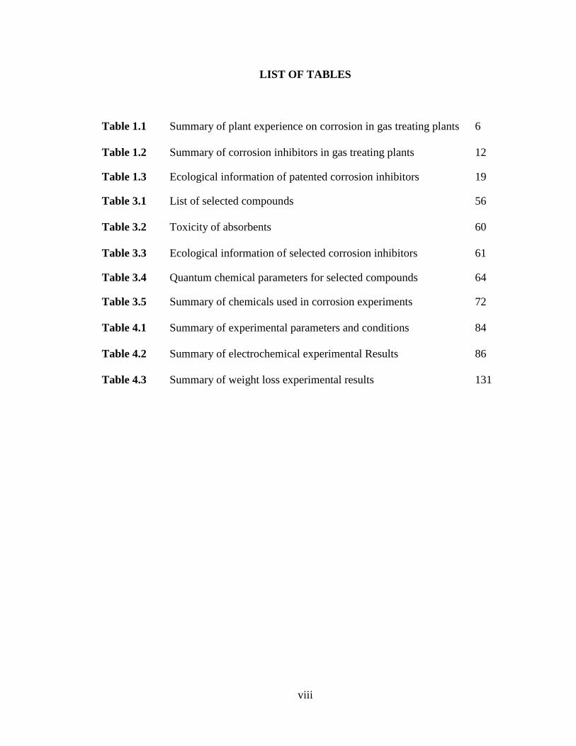
LIST OF TABLES

Table 1.1 Summary of plant experience on corrosion in gas treating plants 6

Table 1.2 Summary of corrosion inhibitors in gas treating plants 12

Table 1.3 Ecological information of patented corrosion inhibitors 19

Table 3.1 List of selected compounds 56

Table 3.2 Toxicity of absorbents 60

Table 3.3 Ecological information of selected corrosion inhibitors 61

Table 3.4 Quantum chemical parameters for selected compounds 64

Table 3.5 Summary of chemicals used in corrosion experiments 72

Table 4.1 Summary of experimental parameters and conditions 84

Table 4.2 Summary of electrochemical experimental Results 86

Table 4.3 Summary of weight loss experimental results 131

ix

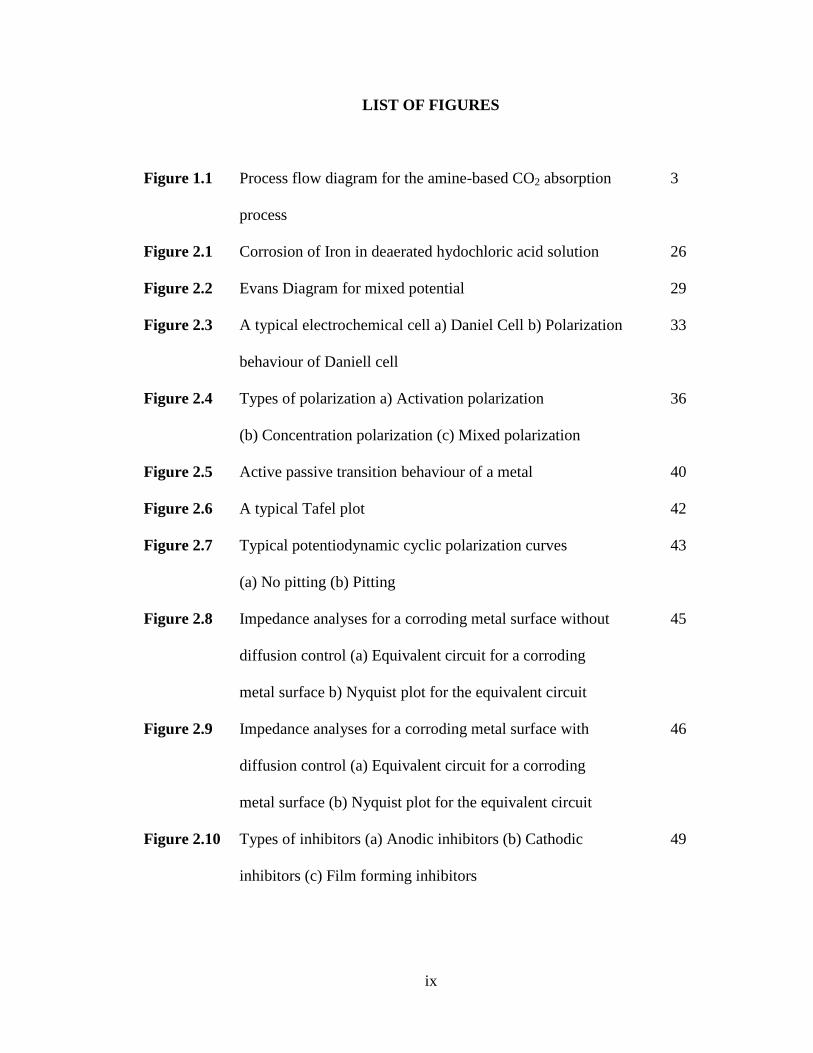
LIST OF FIGURES

Figure 1.1 Process flow diagram for the amine-based CO2 absorption 3

process

Figure 2.1 Corrosion of Iron in deaerated hydochloric acid solution 26

Figure 2.2 Evans Diagram for mixed potential 29

Figure 2.3 A typical electrochemical cell a) Daniel Cell b) Polarization 33

behaviour of Daniell cell

Figure 2.4 Types of polarization a) Activation polarization 36

(b) Concentration polarization (c) Mixed polarization

Figure 2.5 Active passive transition behaviour of a metal 40

Figure 2.6 A typical Tafel plot 42

Figure 2.7 Typical potentiodynamic cyclic polarization curves 43

(a) No pitting (b) Pitting

Figure 2.8 Impedance analyses for a corroding metal surface without 45

diffusion control (a) Equivalent circuit for a corroding

metal surface b) Nyquist plot for the equivalent circuit

Figure 2.9 Impedance analyses for a corroding metal surface with 46

diffusion control (a) Equivalent circuit for a corroding

metal surface (b) Nyquist plot for the equivalent circuit

Figure 2.10 Types of inhibitors (a) Anodic inhibitors (b) Cathodic 49

inhibitors (c) Film forming inhibitors

x

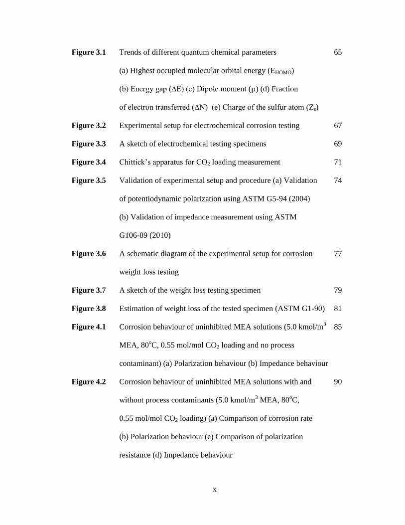
Figure 3.1 Trends of different quantum chemical parameters 65

(a) Highest occupied molecular orbital energy (EHOMO)

(b) Energy gap (∆E) (c) Dipole moment (µ) (d) Fraction

of electron transferred (∆N) (e) Charge of the sulfur atom (Zs)

Figure 3.2 Experimental setup for electrochemical corrosion testing 67

Figure 3.3 A sketch of electrochemical testing specimens 69

Figure 3.4 Chittick’s apparatus for CO2 loading measurement 71

Figure 3.5 Validation of experimental setup and procedure (a) Validation 74

of potentiodynamic polarization using ASTM G5-94 (2004)

(b) Validation of impedance measurement using ASTM

G106-89 (2010)

Figure 3.6 A schematic diagram of the experimental setup for corrosion 77

weight loss testing

Figure 3.7 A sketch of the weight loss testing specimen 79

Figure 3.8 Estimation of weight loss of the tested specimen (ASTM G1-90) 81

Figure 4.1 Corrosion behaviour of uninhibited MEA solutions (5.0 kmol/m3 85

MEA, 80oC, 0.55 mol/mol CO2 loading and no process

contaminant) (a) Polarization behaviour (b) Impedance behaviour

Figure 4.2 Corrosion behaviour of uninhibited MEA solutions with and 90

without process contaminants (5.0 kmol/m3 MEA, 80

oC,

0.55 mol/mol CO2 loading) (a) Comparison of corrosion rate

(b) Polarization behaviour (c) Comparison of polarization

resistance (d) Impedance behaviour

xi

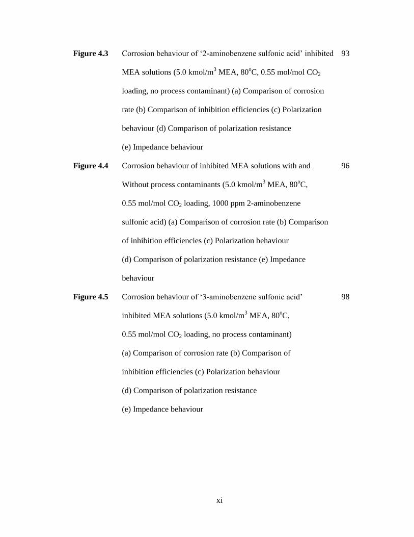
Figure 4.3 Corrosion behaviour of ‘2-aminobenzene sulfonic acid’ inhibited 93

MEA solutions (5.0 kmol/m3 MEA, 80

oC, 0.55 mol/mol CO2

loading, no process contaminant) (a) Comparison of corrosion

rate (b) Comparison of inhibition efficiencies (c) Polarization

behaviour (d) Comparison of polarization resistance

(e) Impedance behaviour

Figure 4.4 Corrosion behaviour of inhibited MEA solutions with and 96

Without process contaminants (5.0 kmol/m3 MEA, 80

oC,

0.55 mol/mol CO2 loading, 1000 ppm 2-aminobenzene

sulfonic acid) (a) Comparison of corrosion rate (b) Comparison

of inhibition efficiencies (c) Polarization behaviour

(d) Comparison of polarization resistance (e) Impedance

behaviour

Figure 4.5 Corrosion behaviour of ‘3-aminobenzene sulfonic acid’ 98

inhibited MEA solutions (5.0 kmol/m3 MEA, 80

oC,

0.55 mol/mol CO2 loading, no process contaminant)

(a) Comparison of corrosion rate (b) Comparison of

inhibition efficiencies (c) Polarization behaviour

(d) Comparison of polarization resistance


xii



oC,


sulfonic acid) (a) Comparison of corrosion rate

(b) Comparison of inhibition efficiencies (c) Polarization



Figure 4.7 Pitting tendency of 3-aminobenzene sulfonic acid in presence of 101

chloride (a) Cyclic polarization curve indicating tendency for

pitting (b) SEM images showing pitted areas (5.0 kmol/m3

MEA, 80oC, 0.55 mol/mol CO2 loading, 1000 ppm

3-aminobenzene sulfonic acid and 10000 ppm chloride)

Figure 4.8 Corrosion behaviour of ‘4-aminobenzene sulfonic acid’ inhibited 103

MEA solutions (5.0 kmol/m3 MEA, 80








oC,


sulfonic acid) (a) Comparison of corrosion rate (b) Comparison

of inhibition efficiencies (c) Polarization behaviour

xiii



Figure 4.10 Corrosion behaviour of ‘sulfapyridine’ inhibited MEA solutions 108

(5.0 kmol/m3 MEA, 80

oC, 0.55 mol/mol CO2 loading, no process

contaminant) (a) Comparison of corrosion rate (b) Comparison of

inhibition efficiencies (c) Polarization behaviour (d) Comparison of

polarization resistance (e) Impedance behaviour



oC,

0.55 mol/mol CO2 loading, 2000 ppm sulfapyridine)

(a) Comparison of corrosion rate (b) Comparison of




Figure 4.12 Corrosion behaviour of ‘sulfanilamide’ inhibited MEA solutions 112




inhibition efficiencies (c) Polarization behaviour (d) Comparison

of polarization resistance (e) Impedance behaviour

Figure 4.13 Corrosion behaviour of ‘sulfolane’ inhibited MEA solutions 114





xiv

(d) Comparison of polarization resistance (e) Impedance

behaviour



oC,

0.55 mol/mol CO2 loading, 2000 ppm sulfolane) (a) Comparison

of corrosion rate (b) Comparison of inhibition efficiencies

(c) Polarization behaviour (d) Comparison of polarization

resistance (e) Impedance behaviour

Figure 4.15 Corrosion behaviour of ‘thiosalicylic acid’ inhibited MEA 119

Solutions (5.0 kmol/m3 MEA, 80






Figure 4.16 Corrosion behaviour of ‘sodium thiosulfate’ inhibited MEA 121

solutions (5.0 kmol/m3 MEA, 80

oC, 0.55 mol/mol CO2 loading,

no process contaminant) (a) Comparison of corrosion rate (b)

Comparison of inhibition efficiencies (c) Comparison of

polarization resistance (d) Impedance behaviour

Figure 4.17 (a) Polarization behaviour of ‘sodium thiosulfate’ inhibited MEA 122


oC, 0.55 mol/mol CO2 loading,

no process contaminant) (b) Working electrode after stable open

circuit potential in presence of sodium thiosulfate (5.0 kmol/m3

xv

MEA, 80oC, 0.55 mol/mol CO2 loading and 1000 ppm sodium

thiosulfate)



oC,

0.55 mol/mol CO2 loading, 1000 ppm sodium thiosulfate)

(a) Comparison of corrosion rate (b) Comparison of inhibition

efficiencies (c) Polarization behaviour (d) Comparison of

polarization resistance (e) Impedance behaviour



oC,

0.55 mol/mol CO2 loading) (a) Comparison of corrosion

rate (b) Comparison of polarization resistance (c) Comparison

of inhibition efficiencies

Figure 4.20 Comparison of corrosion rates of inhibited MEA solutions 132


oC and 0.55 mol/mol CO2 loading,

no process contaminant)

Figure 4.21 Surface analysis of tested specimen after 28 days – (a) SEM 133

images (500X Magnification) (b) EDS spectra (c) XRD spectra



uninhibited)

Figure 4.22 Surface analysis of fresh CS1018 specimen (a) SEM image 135

(Magnification – 500 X) (b) EDS analysis with Wt% of the

element

xvi

Figure 4.23 Comparison of corrosion rates of inhibited MEA solutions 136


oC and 0.55 mol/mol CO2 loading, no

process contaminant)



(5 kmol/m3 MEA, 80


1000 ppm 4-aminobenzene sulfonic acid)



(5kmol/m3 MEA, 80

oC and 0.55 mol/mol CO2 loading, 2000

ppm sulfapyridine)



(5 kmol/m3 MEA, 80


2000 ppm sulfolane)



(5 kmol/m3 MEA, 80

oC and 0.55 mol/mol CO2 loading, 1000 ppm

sodium thiosulfate)

xvii

NOMENCLATURE

a Atomic weight (g/mol)

ap Activity of products

ar Activity of reactants

A Electron affinity (eV)

AC Alternating current

AMP 2-Amino-2-methyl-1-propanol

ASTM American Society for Testing and Materials

C Capacitance (farad)

CAA Clean Air Act

CCS Carbon capture and storage

Cdl Double layer capacitance (μF/cm2)

CE Counter electrode

CEPA Canadian Environmental Protection Act

CR Corrosion rate (mmpy)

CS Carbon steel

CWA Clean Water Act

oC Degree Centigrade

Di Diffusion coefficient

D Density (g/cm3)

DC Direct current

DEA Diethanolamine

xviii

DGA Diglycolamine

DIPA Diisopropanolamine

E Electrode potential (V)

Eo Standard electrode potential (V)

Eb Breakdown potential or pitting potential (V)

Ecorr Corrosion potential (V)

EDS Energy-dispersive X-ray spectroscopy

EHOMO Highest occupied molecular orbital energy (eV)

ELUMO Lowest unoccupied molecular orbital energy (eV)

EIS Electrochemical Impedance Spectroscopy

EPA Environmental Protection Agency

Epp Primary passivation potential (V)

Erev Equilibrium potential (or Reversible potential) (V)

Erp Repassivation potential (V)

∆E Energy gap (eV)

f Frequency (Hz)

F Faraday’s constant (96,500 coulombs per mole)

GHG Greenhouse gas

ΔG Free energy change

HSAB Hard and soft acids and bases

ΔH Enthalpy change

ia Anodic current density (A/cm2)

ic Cathodic current density (A/cm2)

xix

icorr Corrosion current density (A/cm2)

icrit Critical current density (A/cm2)

iL Limiting current density (A/cm2)

io Equilibrium exchange current density (A/cm2)

ipass Passivation current density (A/cm2)

I Ionization potential (eV)

ICDD International Centre for Diffraction Data

IPCC Intergovernmental Panel for Climatic Change

LC50 Lethal concentration (dose large enough to kill 50% of sample animals

under test)

mmpy Millimetre per year

MDEA Methyldiethanolamine

MEA Monoethanolamine

MS Mild carbon steel

n Number of electrons per atom of the species involved in the reaction

n

Hardness (eV)

ΔN Fraction of electrons transferred

OCP Open circuit potential

pow Partition in octanol / water

PAR Princeton Applied Research

PLONOR Poses little or no risk

PM6 Parameterized model number 6

R Gas constant (JK-1

mol-1

)

xx

RE Reference electrode

RP Polarization resistance (ohm cm2)

RS Solution resistance (ohm cm2)

SCC Stress corrosion cracking

SEM Scanning electron microscopy

SS Stainless steel

ΔS Change in entropy

T Absolute temperature (oC)

TEA Triethanolamine

W Warburg impedance (ohm cm2)

WE Working electrode

Wt% Weight percent

XRD X-ray Powder Diffraction

Z Impedance (ohm cm2)

Z' Real impedance (ohm cm2)

Z" Imaginary impedance (ohm cm2)

Zs Charge on the sulfur atom

xxi

Greek Letters:

βa Anodic Tafel slope (mV/decade of current density)

βc Cathodic Tafel slope (mV/decade of current density)

Ƞa Activation polarization (V)

Ƞc Concentration polarization (V)

Ƞdiss Dissolution overpotential (V)

Ƞredn Reduction overpotential (V)

ȠT Total polarization (V)

θ Phase angle (degree)

µ Dipole moment (debye)

χ Electronegativity (eV)

ω Angular frequency

1

1. INTRODUCTION

1.1 Carbon capture from industrial waste gas

The Intergovernmental Panel for Climatic Change (IPCC) has reported that

between 1995 and 2006, eleven out of twelve years were the warmest in the instrumental

record of global surface temperature [IPCC1, 2007]. Melting of glaciers and continual

increases in sea level are the direct effects of global warming. This is mainly attributed to

the increase in the atmospheric concentrations of greenhouse gases (GHGs) in recent

times, which is evident from the fact that GHG emissions now are 70% higher than their

value in the 1970s [IPCC1, 2007]. Particularly, carbon dioxide (CO2) is the most

significant greenhouse gas as its emissions have increased by 80% in the same time

frame, and CO2 represented 77% of the total anthropogenic GHG emissions in 2004

[IPCC1, 2007]. Coal-fired power plants, natural gas processing plants, and manufacturing

industries such as cement, ammonia, and steel plants are some of the major sources of

CO2 emissions [IPCC2, 2005]. Among the above, coal-fired power plants assume specific

importance as they typically contribute to approximately 30% of the total CO2 emissions

[Aaron and Tsouris, 2005].

Carbon capture and storage (CCS) is a technology used to remove CO2 from

industrial flue gas especially from power plants where it can effect a gross reduction of

CO2 emissions by approximately 85 - 95% [IPCC2, 2005]. The CO2 removal can be

accomplished by a number of processes such as membrane separation, adsorption onto

solids, and absorption into liquids. However, the latter is most commonly used for gas

treating applications [Astarita et al., 1983]. The industrial separation of CO2 for natural

2

gas processing and ammonia manufacture by absorption into liquid is a mature

technology and has been successfully used for many decades. However, adaptation of this

technology for flue gas treatment began only in the 1980s [Kittel et al., 2009]. For

example, IMC Global Inc (previously North American chemicals), in Trona, USA,

features a CO2 capture unit that is used to sequester CO2 from flue gas from a coal-fired

power generation plant that started operation in 1978 and is still functioning. Similarly,

Indo-Gulf Corporation, a fertilizer industry in India, features CO2 capture from flue gas

of the ammonia reformer unit that has been operational since 1988 capturing 150 tonnes

CO2/day. Bellingham Cogeneration facility, Massachusetts, USA, produces food grade

CO2 by treating 300 tonnes/day of CO2 from flue gas emitted from an electricity

generation plant since 1991. Sumitomo Chemicals, Japan, treats flue gas generated from

onsite boilers and coal/oil boilers since 1994 with a capacity of 150 tonnes CO2/day. As

illustrated by the above examples of successful and continuous adaptation of this

technology for the past three decades, it is clearly discernible that the flue gas treatment

using absorption into liquid is viewed as a promising technology.

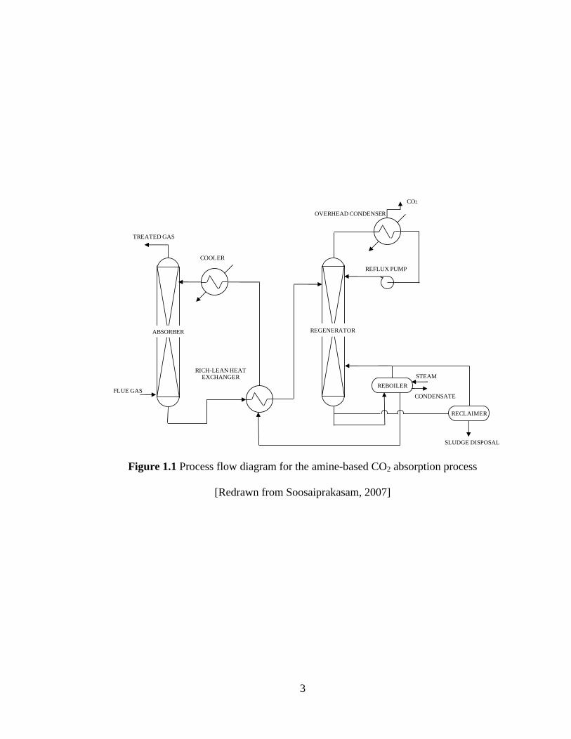
In a typical CO2 absorption process as illustrated in Figure 1.1, a flue gas stream

containing CO2 enters the absorber from the bottom and interacts counter-currently with

down flowing chemical solvent entering from top. CO2 reacts with the solvent and is

absorbed, rendering the gas stream with permissible levels of CO2, and the treated gas

leaves the absorber top. The CO2 loaded rich solvent leaving the bottom of the absorber

passes through the rich-lean heat exchanger where it is preheated and then enters the

regenerator from the top where, on application of heat in the form of steam, the solvent is

stripped of CO2, and the lean solvent is recycled back into the absorber after being cooled

3

Figure 1.1 Process flow diagram for the amine-based CO2 absorption process

[Redrawn from Soosaiprakasam, 2007]

ABSORBER

TREATED GAS

COOLER

RICH-LEAN HEAT EXCHANGER

FLUE GAS

STEAM

CONDENSATE

OVERHEAD CONDENSER

CO2

REFLUX PUMP

REGENERATOR

REBOILER

RECLAIMER

SLUDGE DISPOSAL

4

down to the required operating temperature. A portion of lean solvent is withdrawn at the

reclaimer where it is heated and the vapour mixture containing amine and CO2 are

reintroduced into the regenerator. From the bottom of the reclaimer, a sludge containing

insoluble salts and other chemicals are obtained which is removed for waste handling.

The vapor mixture containing CO2 and water vapor leaves the regenerator and enters the

overhead condenser where most of the water vapor is condensed and recycled back to the

regenerator and the concentrated CO2 leaves the overhead condenser [Aroonwilas, 1996].

A wide range of absorption solvents have been used for CO2 absorption

processes, among which, aqueous alkanolomine-based solvents are the most widely used

absorbents. Alkanolamines can be classified into three categories, namely, primary,

secondary, and tertiary amines. Monoethanolamine (MEA) and diglycolamine (DGA)

belong to the primary type whereas diethanolamine (DEA) and diisopropanolamine

(DIPA) are the secondary type. Methyldiethanolamine (MDEA) and triethanolamine

(TEA) are examples of tertiary amines. In general, primary amines have high reaction

rates with CO2, followed by secondary amines and tertiary amines, respectively [Veawab,

2000]. Since, for flue gas applications, CO2 partial pressures are low and the gas flow rate

is extremely high compared to natural gas processing, the absorption rate has to be

correspondingly faster. With this consideration, MEA shows promise and could well be

the first available solvent absorbent for this application [Kittel et al., 2009; Kittel et al.,

2010].

5

1.2 Corrosion and its impacts

A typical CO2 absorption process can have a number of factors that can cause

operational difficulties, but corrosion is the chief influencing factor from an economic

perspective [Kohl and Nielson, 1997]. Corrosion can greatly influence both economics

and safety associated with the CO2 absorption process. The economic losses are caused

by unplanned downtime, production losses, and reduced equipment life or safety issues

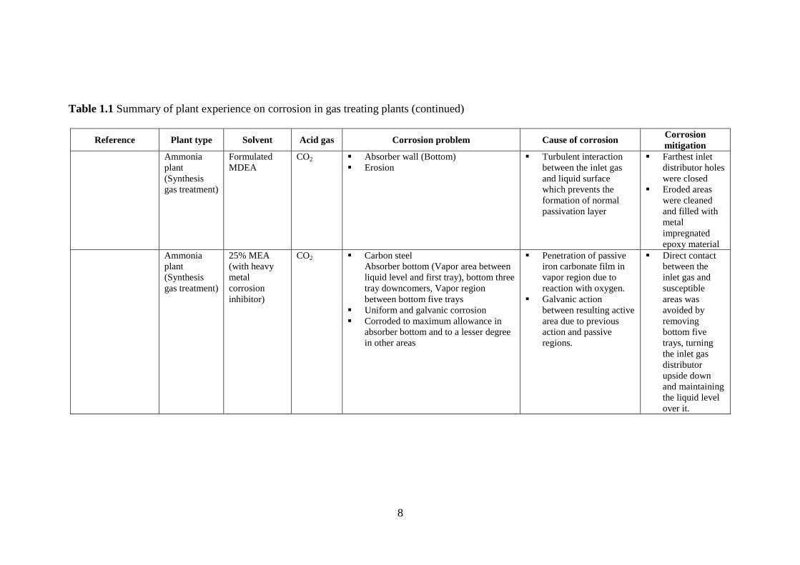
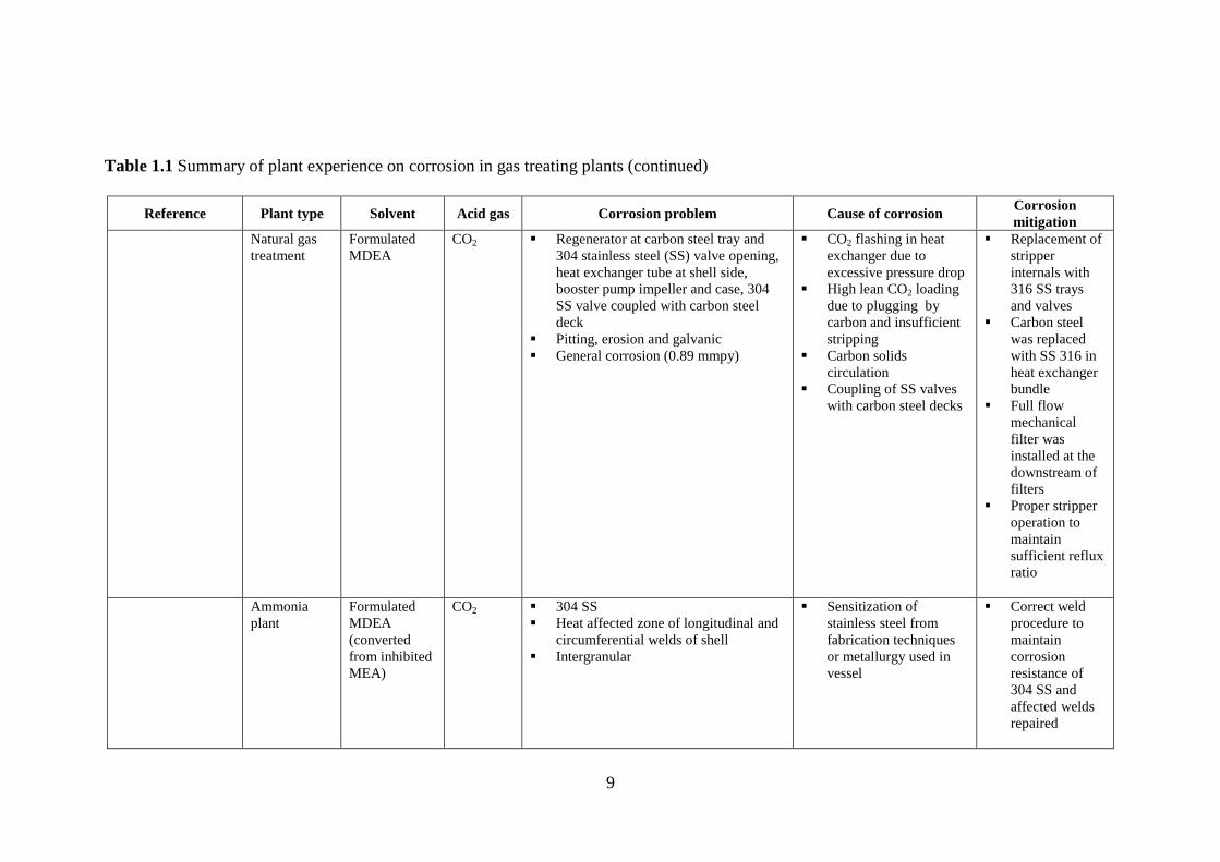
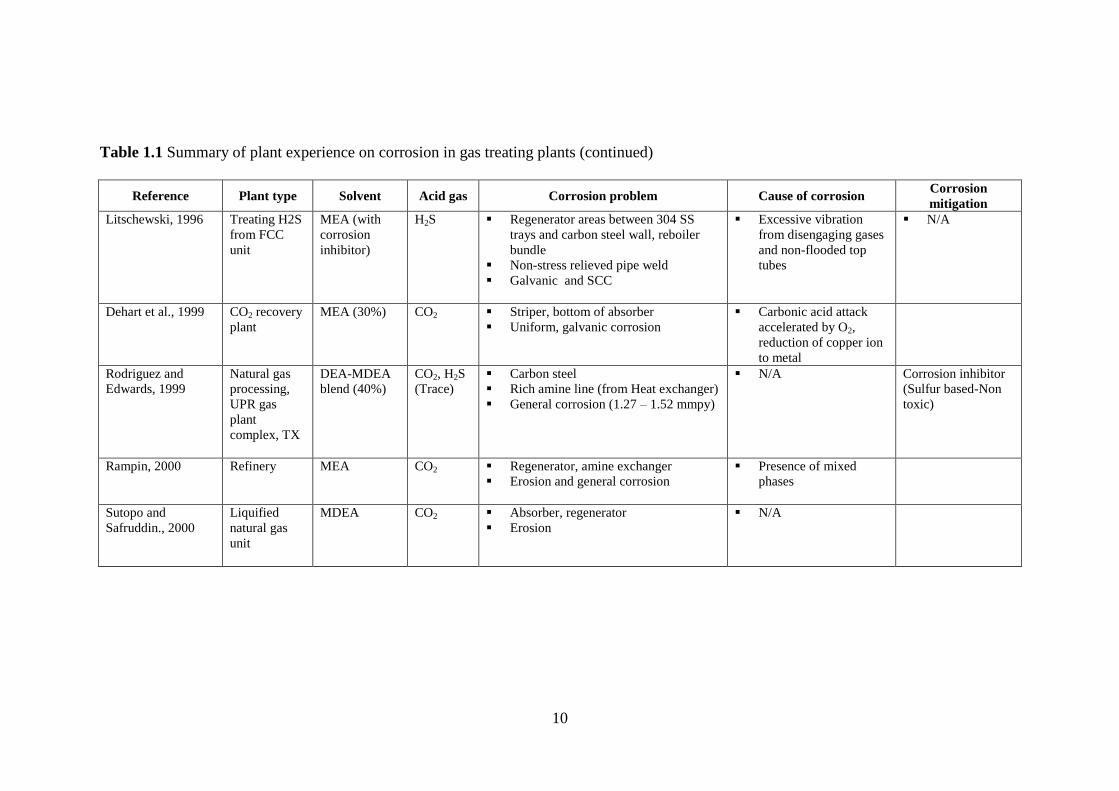
such as injury or death of plant personnel [Dupart et al., 1993]. A summary of plant

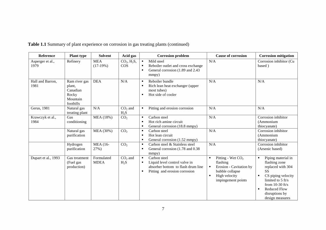
experiences on corrosion in the CO2 absorption process is given in Table 1.1.

From Table 1.1, it can be observed that the absorber bottom, regenerator, heat

exchanger, and associated piping and valves are areas susceptible to severe corrosion.

Both general (uniform) and localized corrosion were observed in CO2 absorption plants.

Localized corrosion such as erosion corrosion due to the presence of foreign particles in

the circulating solution and pitting corrosion are reported to occur in addition to galvanic

corrosion, stress corrosion cracking (SCC), and intergranular corrosion. Acid gas flashing

on walls, high lean loading, high solution velocities, the presence of particulate

contaminants, coupling of dissimilar alloys, and improper metal stress treatment are some

of the reported causes of corrosion. Corrosion mitigation measures include use of

corrosion inhibitors, design measures to reduce acid gas flashing, and replacement of

carbon steel with corrosion resistant alloys in the heat exchanger and regenerator areas

(trays and valves) in some cases.

6

Table 1.1 Summary of plant experience on corrosion in gas treating plants

Reference Plant type Solvent Acid gas Corrosion problem Cause of corrosion Corrosion

mitigation

Dingman et al.,

1966

Sour gas

treating plant

MEA CO2 and

H2S

Rich-lean heat exchanger, solution

letdown valve, piping downstream

letdown valve, upper portion of

regenerator

Erosion corrosion

Flashing of acid gas

from hot surface

High solution velocity

Change in direction of

fluid flow

Contamination with

solids such as iron

oxide, iron sulfide, mill

scale and sand

N/A

Smith and

Younger., 1972

Twenty-four

Sour gas

treating plants

in western

Canada

DEA CO2 and

H2s

Erosion corrosion

- Rich lean heat exchanger

- Regenerator

- Reboiler-vapor line and letdown

- Rich solution piping

Stress corrosion cracking

- Stainless steel heat exchanger

Contamination of

foreign particles in

circulating solution

High solution velocity

(5.5 ft/s)

Insufficient liquid level

over tight tube spacing

in reboiler and heat

exchanger

Chloride ion evolved

from gasket material

used between plates

N/A

Heisler and Weiss,

1975

Natural gas

treating plant,

Aderklaa,

Austria

MEA CO2 and

H2S

Tray type regenerator including wall

internal, downcomer, circumferential

joint, weld seam and joint, and tray

Uniform, pitting, erosion

Cavity in vapor flash N/A

Schmeal et al., 1978 Sour gas

treating plant

Sulfinol

(DIPA +

sulfolane)

CO2 and

H2S

Absorber below 5th

tray

Pitting

Acid gas flashing N/A

7

Table 1.1 Summary of plant experience on corrosion in gas treating plants (continued)

Reference Plant type Solvent Acid gas Corrosion problem Cause of corrosion Corrosion mitigation

Asperger et al.,

1979

Refinery MEA

(17-19%)

CO2, H2S,

COS

Mild steel

Reboiler outlet and cross exchange

General corrosion (1.89 and 2.43

mmpy)

N/A Corrosion inhibitor (Cu

based )

Hall and Barron,

1981

Ram river gas

plant,

Canadian

Rocky

Mountain

foothills

DEA N/A Reboiler bundle

Rich lean heat exchanger (upper

most tubes)

Hot side of cooler

N/A N/A

Gerus, 1981 Natural gas

treating plant

N/A CO2 and

H2S

Pitting and erosion corrosion N/A N/A

Krawczyk et al.,

1984

Gas

conditioning

MEA (18%) CO2 Carbon steel

Hot rich amine circuit

General corrosion (18.8 mmpy)

N/A Corrosion inhibitor

(Ammonium

thiocyanate)

Natural gas

purification

MEA (30%) CO2 Carbon steel

Hot lean circuit



(Ammonium

thiocyanate)

Hydrogen

purification

MEA (16-

27%)

CO2 Carbon steel & Stainless steel

General corrosion (1.78 and 0.38

mmpy)


(Arsenic based)

Dupart et al., 1993 Gas treatment

(Fuel gas

production)

Formulated

MDEA

CO2 and

H2S

Carbon steel

Liquid level control valve in

absorber bottom to flash drum line

Pitting and erosion corrosion

Pitting - Wet CO2

flashing

Erosion - Cavitation by

bubble collapse

High velocity

impingement points

Piping material in

flashing zone

replaced with 304

SS

CS piping velocity

limited to 5 ft/s

from 10-30 ft/s

Reduced Flow

disruptions by

design measures

8



mitigation

Ammonia

plant

(Synthesis

gas treatment)

Formulated

MDEA

CO2 Absorber wall (Bottom)

Erosion

Turbulent interaction

between the inlet gas

and liquid surface

which prevents the

formation of normal

passivation layer

Farthest inlet

distributor holes

were closed

Eroded areas

were cleaned

and filled with

metal

impregnated

epoxy material

Ammonia

plant

(Synthesis

gas treatment)

25% MEA

(with heavy

metal

corrosion

inhibitor)

CO2 Carbon steel

Absorber bottom (Vapor area between

liquid level and first tray), bottom three

tray downcomers, Vapor region

between bottom five trays

Uniform and galvanic corrosion

Corroded to maximum allowance in

absorber bottom and to a lesser degree

in other areas

Penetration of passive

iron carbonate film in

vapor region due to

reaction with oxygen.

Galvanic action

between resulting active

area due to previous

action and passive

regions.

Direct contact

between the

inlet gas and

susceptible

areas was

avoided by

removing

bottom five

trays, turning

the inlet gas

distributor

upside down

and maintaining

the liquid level

over it.

9



mitigation

Natural gas

treatment

Formulated

MDEA

CO2 Regenerator at carbon steel tray and

304 stainless steel (SS) valve opening,

heat exchanger tube at shell side,

booster pump impeller and case, 304

SS valve coupled with carbon steel

deck

Pitting, erosion and galvanic


CO2 flashing in heat

exchanger due to

excessive pressure drop

High lean CO2 loading

due to plugging by

carbon and insufficient

stripping

Carbon solids

circulation

Coupling of SS valves

with carbon steel decks

Replacement of

stripper

internals with

316 SS trays

and valves

Carbon steel

was replaced

with SS 316 in

heat exchanger

bundle

Full flow

mechanical

filter was

installed at the

downstream of

filters

Proper stripper

operation to

maintain

sufficient reflux

ratio

Ammonia

plant

Formulated

MDEA

(converted

from inhibited

MEA)

CO2 304 SS

Heat affected zone of longitudinal and

circumferential welds of shell

Intergranular

Sensitization of

stainless steel from

fabrication techniques

or metallurgy used in

vessel

Correct weld

procedure to

maintain

corrosion

resistance of

304 SS and

affected welds

repaired

10



mitigation

Litschewski, 1996 Treating H2S

from FCC

unit

MEA (with

corrosion

inhibitor)

H2S Regenerator areas between 304 SS

trays and carbon steel wall, reboiler

bundle

Non-stress relieved pipe weld

Galvanic and SCC

Excessive vibration

from disengaging gases

and non-flooded top

tubes

N/A

Dehart et al., 1999 CO2 recovery

plant

MEA (30%) CO2 Striper, bottom of absorber

Uniform, galvanic corrosion

Carbonic acid attack

accelerated by O2,

reduction of copper ion

to metal

Rodriguez and

Edwards, 1999

Natural gas

processing,

UPR gas

plant

complex, TX

DEA-MDEA

blend (40%)

CO2, H2S

(Trace)

Carbon steel

Rich amine line (from Heat exchanger)

General corrosion (1.27 – 1.52 mmpy)


(Sulfur based-Non

toxic)

Rampin, 2000 Refinery MEA CO2 Regenerator, amine exchanger

Erosion and general corrosion

Presence of mixed

phases

Sutopo and

Safruddin., 2000

Liquified

natural gas

unit

MDEA CO2 Absorber, regenerator

Erosion

N/A

11

1.3 Corrosion inhibitors

There are many alternative approaches to mitigating corrosion in CO2

absorption plants, such as proper equipment and process design, use of corrosion

resistant materials, side stream removal of particulate matters from amine solution,

and use of corrosion inhibitors. Among these, the use of corrosion inhibitors is

considered the most economical, mainly because it requires no major process

modification [Kohl and Nielson, 1997; Dupart et al., 1993; Veawab, 2000]. From the

plant experiences detailed in Table 1.1, it can be seen that despite the usage of

corrosion inhibitors, corrosion can still occur due to certain design problems such as

coupling of dissimilar metals and acid gas flashing in selected areas [Dupart et al.,

1993]. Hence, corrosion inhibitors in combination with one or all of the above

approaches have to be deployed for effective corrosion reduction. This thesis work

focused mainly on corrosion inhibitors.

A corrosion inhibitor is defined as a chemical substance that, when added in

small concentrations to the fluid phase of a corroding environment, are capable of

retarding corrosion by interacting either with the metal surface or the environment

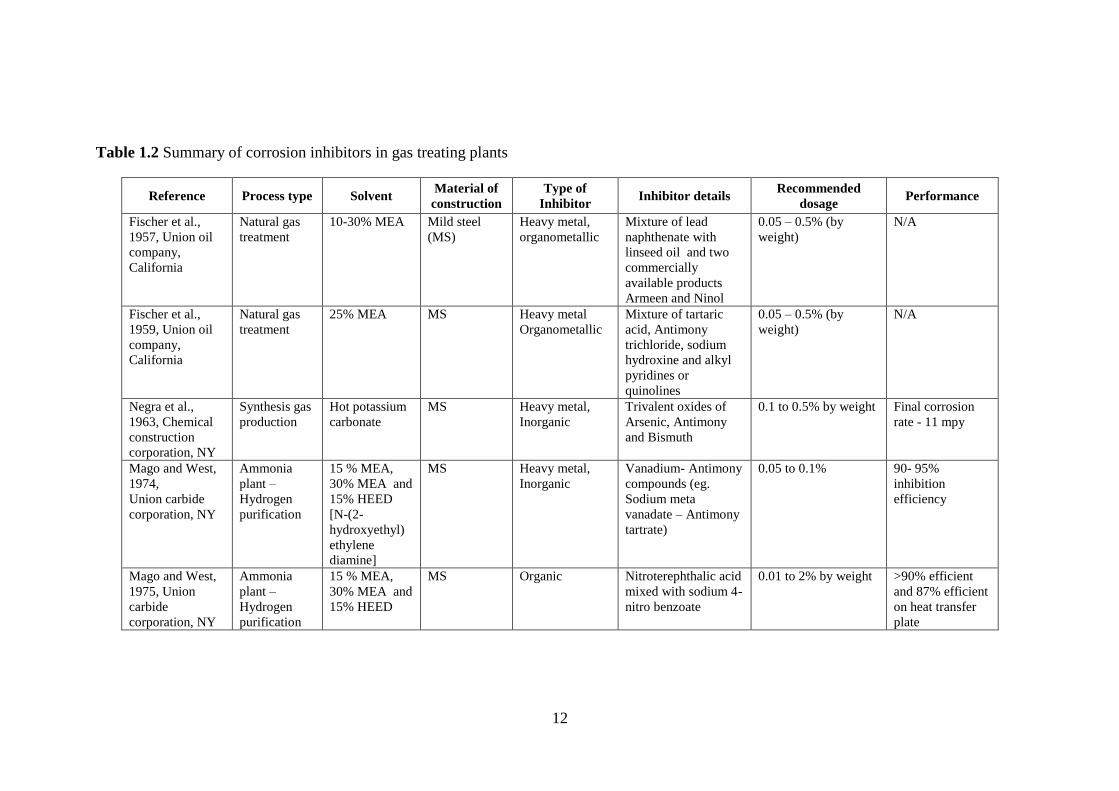
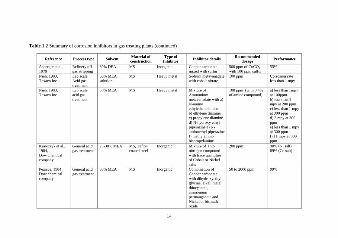
[Sastri, 2001]. A wide array of corrosion inhibitors were tested and patented for gas

treating applications over the past fifty years (Table 1.2), but the most effective ones

are based on heavy metals such as arsenic and vanadium [Dupart et al., 1993]. For a

period of around two decades, beginning in 1957, several heavy metal inhibitors such

as lead-based, antimony and bismuth-based, arsenic, vanadium, and tin-based

compounds were tested and patented. Despite being very effective inhibitors, their

usage was restricted because they are toxic inorganic compounds, which makes their

disposal difficult and costly [Kohl and Nielson, 1997]. As a result, a shift in trend

towards development of environmentally-friendly corrosion inhibitors was inevitable.

12

Table 1.2 Summary of corrosion inhibitors in gas treating plants

Reference Process type Solvent Material of

construction

Type of

Inhibitor Inhibitor details

Recommended

dosage Performance

Fischer et al.,

1957, Union oil

company,

California

Natural gas

treatment

10-30% MEA Mild steel

(MS)

Heavy metal,

organometallic

Mixture of lead

naphthenate with

linseed oil and two

commercially

available products

Armeen and Ninol

0.05 – 0.5% (by

weight)

N/A

Fischer et al.,

1959, Union oil

company,

California

Natural gas

treatment

25% MEA MS Heavy metal

Organometallic

Mixture of tartaric

acid, Antimony

trichloride, sodium

hydroxine and alkyl

pyridines or

quinolines

0.05 – 0.5% (by

weight)

N/A

Negra et al.,

1963, Chemical

construction

corporation, NY

Synthesis gas

production

Hot potassium

carbonate

MS Heavy metal,

Inorganic

Trivalent oxides of

Arsenic, Antimony

and Bismuth

0.1 to 0.5% by weight Final corrosion

rate - 11 mpy

Mago and West,

1974,

Union carbide

corporation, NY

Ammonia

plant –

Hydrogen

purification

15 % MEA,

30% MEA and

15% HEED

[N-(2-

hydroxyethyl)

ethylene

diamine]

MS Heavy metal,

Inorganic

Vanadium- Antimony

compounds (eg.

Sodium meta

vanadate – Antimony

tartrate)

0.05 to 0.1% 90- 95%

inhibition

efficiency

Mago and West,

1975, Union

carbide

corporation, NY

Ammonia

plant –

Hydrogen

purification

15 % MEA,

30% MEA and

15% HEED

MS Organic Nitroterephthalic acid

mixed with sodium 4-

nitro benzoate

0.01 to 2% by weight >90% efficient

and 87% efficient

on heat transfer

plate

13

Table 1.2 Summary of corrosion inhibitors in gas treating plants (continued)


construction

Type of


Recommended

dosage Performance

Mago, 1976,

Union carbide

corporation, NY

Lab scale

acid gas

treatment

Hot potassium

carbonate (with

5%

bicarbonate)

MS (Cold

rolled)

Heavy metal,

Inorganic

a)Vanadium

compounds

b) Antimony

compounds

c) Combination of

above

0.01 to 2% a) -400%

(aggravated

corrosion)

b) -70%

(aggravated

corrosion)

c) 84-90%

Mago and West,

1976,

Union carbide

corporation, NY

Ammonia

plant –

Hydrogen

purification

30% MEA,

30% 1:1

MEA:HEED

MS Heavy metal,

Inorganic

Stannous tartarate 0.01 to 2% 80-95%

Davidson et al.,

1978, Dow

chemical

company

Natural or

synthesis gas

treatment

(pilot plant)

30% MEA MS Inorganic, Reaction product of

copper and sulfur

yielding compounds

with

Monoethanolamine

20 – 20000 ppm

(0.002 – 2%)

N/A

Asperger and

Clouse, 1978,

Dow chemical

company

Natural or

synthesis gas

treatment

30% MEA MS Organic Tetradecyl

polyalkylpyridinium

bromide with

polyethylene

polyamine

100 ppm 91%

Clouse and

Asperger, 1978,

Dow chemical

company

Lab scale

Acid gas

treatment

30% MEA MS Organic +

Inorganic

Tetradecyl

polyalkylpyridinium

bromide with thio

urea and cobalt

acetate

50 ppm (with10-50

ppm cobalt acetate)

96%

Clouse and

Asperger, 1978,

Dow chemical

company

Lab scale

Acid gas

treatment

30% MEA MS Organic Tetradecyl

polyalkylpyridinium

with a) Thio urea

b) Thiocyanate or c)

Thionicotinamide

50 ppm a) 77%

b) 91%

c) 92%

14



construction

Type of


Recommended

dosage Performance

Asperger et al.,

1979

Refinery off-

gas stripping

30% DEA MS Inorganic Copper carbonate

mixed with sulfur

500 ppm of CuCO3

with 100 ppm sulfur

55%

Nieh, 1983,

Texaco Inc

Lab scale

Acid gas

treatment

50% MEA

solution

MS Heavy metal Sodium metavanadate

with cobalt nitrate

100 ppm Corrosion rate

less than 1 mpy

Nieh, 1983,

Texaco Inc

Lab scale

acid gas

treatment

50% MEA MS Heavy metal Mixture of

Ammonium

metavanadate with a)

N-amino

ethylethanolamine

b) ethylene diamine

c) propylene diamine

d) N-hydroxy ethyl

piperazine e) N-

aminoethyl piperazine

f) methylamino

bispropylamine

100 ppm (with 0.4%

of amine compound)

a) less than 1mpy

at 100ppm

b) less than 1

mpy at 200 ppm

c) less than 1 mpy

at 300 ppm

d) 3 mpy at 300

ppm

e) less than 1 mpy

at 300 ppm

f) 11 mpy at 300

ppm

Krawczyk et al.,

1984,

Dow chemical

company

General acid

gas treatment

25-30% MEA MS, Teflon

coated steel

Inorganic Mixture of Thio

nitrogen compound

with trace quantities

of Cobalt or Nickel

salts

200 ppm 90% (Ni salt)

89% (Co salt)

Pearsce, 1984

Dow chemical

company

General acid

gas treatment

80% MEA MS Inorganic Combination of

Copper carbonate

with dihydroxyethyl

glycine, alkali metal

thiocyanate,

ammonium

permanganate and

Nickel or bismuth

oxide

50 to 2000 ppm 99%

15



construction

Type of


Recommended

dosage Performance

Dupart et al.,

1984,

Dow chemical

Company

Natural &

synthesis gas

treatment

30% MEA

solution

MS, Stainless

steel (SS)

type 304, type

316 and

Monel

Inorganic Combination of

Ammonium

thiocyanate, Bismuth

citrate and Nickel

sulfate

Greater than 50 ppm

of thiocyanate (with

Bismuth citrate 1-100

ppm)

93.6% efficiency

Jones and Alkire,

1985,

Standard oil

company

Natural &

synthesis gas

treatment

20 – 60% DEA MS Organic-

Inorganic

Dodecylbenzyl

chloride with

alkylpyridine still

bottoms and Nickel

acetate

2000 ppm (with 35

ppm Ni compound)

Maximum

efficiency of

93.1%

Henson et al.,

1986,

Dow chemical

company

Refinery gas

conditioning

30% MEA Carbon steel

(CS)

Organic-

Inorganic

Mixture of

Aminoethyl

piperazine-

Formaldehyde-

thiourea polymer and

Nickel sulfate

5000 ppm As close as 100%

reported

Trevino, 1987,

Hylsa, S.A

Gas

processing

25 – 30%

MEA

CS Inorganic Mixture of cupric

oxide and Zinc sulfate

with bronze pieces (to

maintain Copper and

Zinc concentration)

Copper - 1-500ppm

Zinc – 100-500 ppm

80% efficiency at

regenerator top

and 90% at

absorber bottom

Sekine et al.,

1992, Dept. of

Industrial

chemistry,

University of

Tokyo

General acid

gas treatment

23% hot

potassium

carbonate

MS and SS Organic Combination of

following a)2-

Aminothiophenol

(ATP) b) 1-

Hydroxyethylidene

bisphosphonic acid

(HEDP) and c)

Diethanolamine

(DEA)

a) 10 ppm

b) 100ppm

c) 3%

Maximum

efficiency of 92%

for SS41 and

95% for SS104

16


Reference Process

type Solvent

Material of

construction

Type of


Recommended

dosage Performance

Minevski and

Labmbousy, 1998,

BetzDearborn Inc

General

acid gas

treatment

18% MEA (140

ppm sulfuric acid,

150 ppm oxalic

acid, 240 ppm

formic acid and 30

ppm sodium

chloride)

MS Organic 1,6 Hexanedithiol

with cyclohexanethiol

or decanethiol or

dodecane thiol is used

25 – 100 ppm (with

less than 1% by

weight of thiol)

Maximum

efficiency of

around 90% when

only CO2 is

present and 75%

when H2S is also

present.

Minevski, 2000,

BetzDearborn Inc

General

acid gas

treatment

18% MEA (140

ppm sulfuric acid,

150 ppm oxalic

acid, 240 ppm

formic acid and 30

ppm sodium

chloride)

MS Organic Combination of

Thiomorpholine with

Phthalic acid

500 – 2000 ppm Maximum

effiency of about

92%

Veawab et al., 2001,


Industrial

gas

treatment

3M MEA CS Organic a)Amine-based

b) Sulfoxide based

c) Carboxylic acid

based

a) 1000 ppm

b) 1000 ppm

c) 5000 ppm

a) around 75%

b) over 75%

c)98%

Veldman and Trahan,

2001, Coastal

Chemical Co

Natural

gas plant

and

Refinery

Hydrogen

treatment

50% MDEA

solution

MS and SS Heavy metal Sodium molybdate in

presence of

hydroquinone,

ethylketoxime and

diethylhydroxyl

amine

3.5% by weight Over 99%

Chang et al., 2008,

GE Betz Inc

General

acid gas

treatment

25% MEA and

30% DEA

CS Organic Polythia ether

compounds

10-20 ppm 96% for DEA and

99% for MEA

Soosaiprakasam and

Veawab, 2009,


General

acid gas

treatment

MEA (5M, 7M

and 9M)

CS Inorganic Copper carbonate 250 ppm Above 80%

17

New corrosion inhibitors were initially relatively less toxic either because of

the choice of the chemical compounds or by combination of heavy metals with less

toxic compounds. Davidson et al., 1978, registered a patent for the claim of copper

and sulfur-based chemical compounds as corrosion inhibitors that were less toxic than

heavy metal corrosion inhibitors. Copper carbonate in combination or alone has been

suggested a potential corrosion inhibitor since 1979 [Asperger et al., 1979; Pearsce,

1984; Trevino, 1987; Soosaiprakasam and Veawab, 2009]. Many organic compounds

such as pyridinium-based, piperazine-based, thiophenol- and thiol-based, and amine

and carboxylic acid-based compounds were also reported with comparable inhibition

efficiencies of around 90%. Inorganic inhibitors were generally used in the

concentration range of 20 – 2000 ppm whereas organic inhibitors were in the range of

100 – 20000 ppm. During the initial development period, only inhibition efficiency

was of primary concern. However, increased environmental awareness has led to the

choice of corrosion inhibitors that are not only effective but also eco-friendly.

1.4 Research motivation

Disposal of toxic chemicals has resulted in significant damage to human and

environmental health and, based on those experiences, environmental awareness has

seen tremendous growth in the last few decades. As a result, a number of initiatives

were taken across the world. For instance, in the United States, for a period of over

100 years, since the late 1800s, only 20 environmental laws were passed. However, in

the few decades that followed, over 120 environmental regulatory laws were set in

place. Consequently, the cost of compliance with those environmental regulations

through waste treatment, control, and disposal were high and has been estimated to be

in the range of 100-150 billion USD per year for the affected industries [Anastas and

18

Williamson, 1998; Doble and Kruthiventi, 2007]. In Canada, usage of toxic

substances is regulated by the Canadian Environmental Protection Act (CEPA). For

example, inorganic arsenic and cadmium compounds are classified as carcinogenic

and considered toxic and were listed as CEPA 1999 Schedule-I compounds, and as a

result, their usage was banned. In the USA, the Environmental Protection Agency

(EPA) regulates the usage of chemicals through the Clean Water Act (CWA) and

Clean Air Act (CAA). In Europe, an environmental regulatory mechanism OSPAR

was established by fifteen Northeast Atlantic nations by unifying their policies in the

1972 Oslo convention against waste dumping to protect the marine environment. This

was later broadened to cover land-based pollutant sources and offshore industries in

the Paris Convention of 1974 [OSPAR, 2011]. As per the guidelines set by OSPAR

for environmentally-friendly chemicals, for a chemical to be listed in PLONOR

(poses little or no risk), two out of three of the following requirements has to be

satisfied with its biodegradability being superior to 20% in 28 days: a)

Biodegradability (>60% in 28 days), b) Toxicity [Lethal concentration (LC50) or

Effective concentration (EC50)] > 1mg/L for inorganic species and (LC50 or EC50 >

10mg/L for organic species) where LC50 or EC50 is the dose large enough to kill 50%

of sample animals under test; and c) Bioaccumulation ( logpow < 3 where pow is the

partition in octanol/water)

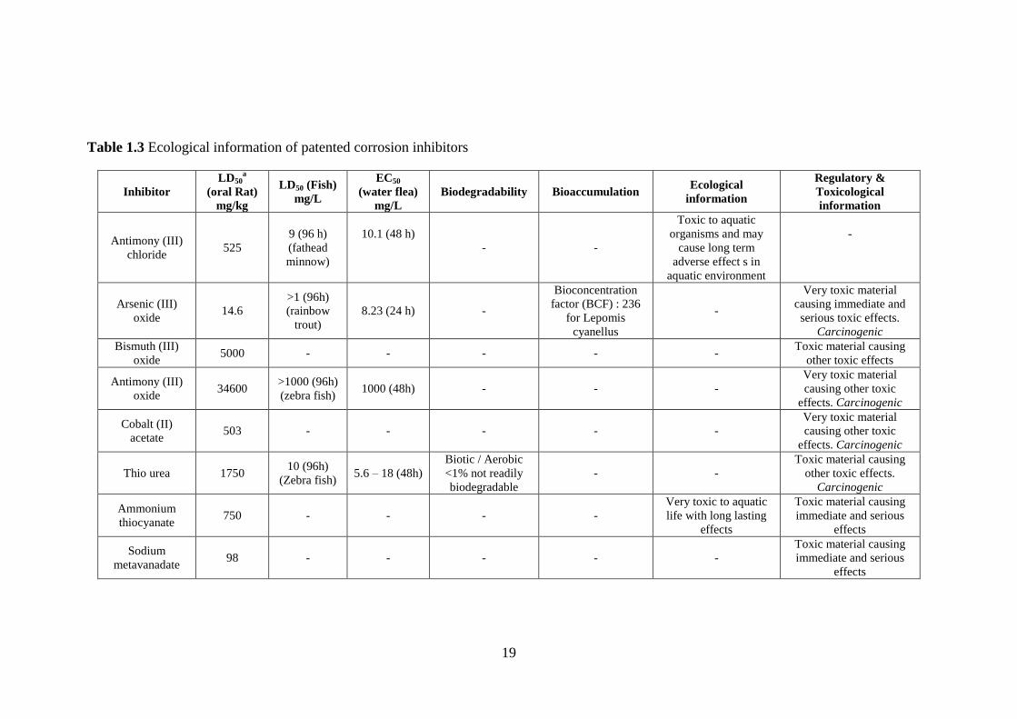
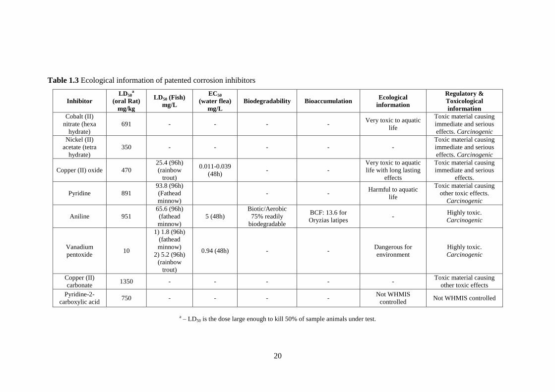
Based on the above OSPAR guidelines, it can be observed from Table 1.3 that

most corrosion inhibitors that are used, tested, and patented are non-environmentally

friendly. For instance, Antimony (III) oxide, arsenic oxide, cobalt acetate, thiourea,

aniline, pyridine, and vanadium compounds are toxic and carcinogenic. Hence, there

is a need to develop an environmentally-friendly corrosion inhibitor that can replace

the present highly toxic ones and also provide comparable inhibition efficiencies.

19

Table 1.3 Ecological information of patented corrosion inhibitors

Inhibitor

LD50a

(oral Rat)

mg/kg

LD50 (Fish)

mg/L

EC50

(water flea)

mg/L

Biodegradability Bioaccumulation Ecological

information

Regulatory &

Toxicological

information

Antimony (III)

chloride 525

9 (96 h)

(fathead

minnow)

10.1 (48 h)

- -

Toxic to aquatic

organisms and may

cause long term

adverse effect s in

aquatic environment

-

Arsenic (III)

oxide 14.6

>1 (96h)

(rainbow

trout)

8.23 (24 h) -

Bioconcentration

factor (BCF) : 236

for Lepomis

cyanellus

-

Very toxic material

causing immediate and

serious toxic effects.

Carcinogenic

Bismuth (III)

oxide 5000 - - - - -

Toxic material causing

other toxic effects

Antimony (III)

oxide 34600

>1000 (96h)

(zebra fish) 1000 (48h) - - -

Very toxic material

causing other toxic

effects. Carcinogenic

Cobalt (II)

acetate 503 - - - - -

Very toxic material

causing other toxic


Thio urea 1750 10 (96h)

(Zebra fish) 5.6 – 18 (48h)

Biotic / Aerobic

<1% not readily

biodegradable

- -


other toxic effects.

Carcinogenic

Ammonium

thiocyanate 750 - - - -

Very toxic to aquatic

life with long lasting

effects


immediate and serious

effects

Sodium

metavanadate 98 - - - - -



effects

20

Table 1.3 Ecological information of patented corrosion inhibitors

Inhibitor

LD50a

(oral Rat)

mg/kg

LD50 (Fish)

mg/L

EC50

(water flea)

mg/L

Biodegradability Bioaccumulation Ecological

information

Regulatory &

Toxicological

information

Cobalt (II)

nitrate (hexa

hydrate)

691 - - - - Very toxic to aquatic

life




Nickel (II)

acetate (tetra

hydrate)

350 - - - - -




Copper (II) oxide 470

25.4 (96h)

(rainbow

trout)

0.011-0.039

(48h) - -

Very toxic to aquatic

life with long lasting

effects



effects.

Pyridine 891

93.8 (96h)

(Fathead

minnow)

- - Harmful to aquatic

life


other toxic effects.

Carcinogenic

Aniline 951

65.6 (96h)

(fathead

minnow)

5 (48h)

Biotic/Aerobic

75% readily

biodegradable

BCF: 13.6 for

Oryzias latipes -

Highly toxic.

Carcinogenic

Vanadium

pentoxide 10

1) 1.8 (96h)

(fathead

minnow)

2) 5.2 (96h)

(rainbow

trout)

0.94 (48h) - - Dangerous for

environment

Highly toxic.

Carcinogenic

Copper (II)

carbonate 1350 - - - - -


other toxic effects

Pyridine-2-

carboxylic acid 750 - - - -

Not WHMIS

controlled Not WHMIS controlled

a – LD50 is the dose large enough to kill 50% of sample animals under test.

Many previous works have attempted to search for a suitable green corrosion

inhibitor for absorption-based gas treating plants. In general, it was observed that organic

inhibitors are much more environmentally friendly than inorganic inhibitors [Veawab et

al, 2001]. Asperger and Clouse [1978] have patented two different organic corrosion

inhibitors based on polyalkyl pyridinium. Minevsky and Lambousy [1998] have reported

a corrosion inhibitor based on organic thiol and dithiols. Minevsky [2001] has also

reported a thiomorpholine-based corrosion inhibitor. Similarly, Veawab et al. [2001]

have reported eight organic inhibitors based on carboxylic acid, sulfoxide, and amines

that are all reportedly less toxic than the conventional vanadium-based inhibitors and

comparably efficient. All these suggest that searching for a potential corrosion inhibitor

that is environmentally friendly as well as efficient compared to conventional corrosion

inhibitors has been a continuous process, but no compound yet has emerged as a

satisfactory candidate for replacement of conventional corrosion inhibitors.

1.5 Research objectives and scope

The most effective corrosion inhibitors patented are not eco-friendly, as can be

seen in Table 1.3. This leads to an objective to search for an environmentally-friendly

corrosion inhibitor with comparable inhibition performance that can replace conventional

highly toxic corrosion inhibitors. To achieve this objective, this work was implemented

through 4 tasks:

i. Selection of chemical compounds for testing as corrosion inhibitors

On understanding of chemistry, it is possible to select a chemical

compound that can best interact with the metal (surface) to be protected. On that

22

basis, in this work, thirteen organic compounds were selected and studied. That

also includes the structural isomers of some of the selected compounds that have

the same functional groups and reaction centers as those of the parent compound.

ii. Analysis of the inhibitor for eco-friendliness

Since the primary focus of this work is to search for an environmentally-

friendly corrosion inhibitor, ecological analysis assumes primary importance.

Selected compounds were evaluated based on their toxicity values in terms of

LD50 (Lethal dosage to kill 50% of sample animals under test) and other available

ecological data.

iii. Theoretical analysis of the inhibitor for performance

Quantum chemical studies are extensively used in corrosion inhibitor

development mainly because it can provide a predictive capability of corrosion

inhibition performance of different compounds. In this work, an attempt was

made to evaluate compounds on that basis.

iv. Experimental testing, Evaluation, and Recommendation

Final shortlisted compounds were subjected to experimental analysis to

evaluate the corrosion inhibition performance of these compounds and understand

the mechanisms of interaction. Corrosion inhibitors were evaluated based on their

effect on corrosion rate of carbon steel, which is a common material of

construction in amine-based CO2 capture plants. Inhibitors were

electrochemically tested at different concentrations ranging from as low as 250

ppm to 10,000 ppm. Also, the effect of the presence of possible process

contaminants on corrosion inhibition performance was studied. Their performance

23

was evaluated based on various experimentally-obtained parameters such as

corrosion rate, polarization resistance, corrosion current, and inhibition

efficiencies. Weight loss testing was carried out to corroborate the results

obtained from the electrochemical tests.

Based on the above results, those compounds that manifested good potential for corrosion

inhibition were recommended for further study.

24

2. FUNDAMENTALS OF CORROSION AND CORROSION INHIBITION

Knowledge of fundamentals of corrosion is imperative to understanding the

mechanism of corrosion based on which a congruent selection of corrosion preventive

method can be made. It is also useful in the prognosis of corrosion behaviour of different

metals under variegated conditions. In order to reasonably understand the process of

corrosion, it is necessary to understand the thermodynamics and associated kinetics of the

corroding system under investigation.

2.1 Thermodynamic aspects of corrosion

Thermodynamic principles can be used to ascertain the driving force and

spontaneous direction for any reaction. In general, driving force is characterized as the

balance between the effect of change in energy (enthalpy, ∆H) and the effect of change in

thermodynamic probability (entropy, ∆S). Free energy change (∆G) is used to quantify

the above and at constant temperature can be expressed as

∆G = ∆H - T∆S (2.1)

where T is the absolute temperature. Only those reactions that lower the energy of the

system can be spontaneous, which implies that the free energy change will be negative

for a spontaneous reaction [ASM Handbook (13), 1987].

2.1.1 Origin of electrode potential

Corrosion of metals, especially in aqueous environments, is electrochemical in

nature involving at least two electrochemical reactions occurring concurrently on the

25

metal surface. The corroding metal surface is the electrode and the aqueous medium,

which acts as an ionic conductor, is the electrolyte. Thus, when an electrode is brought in

contact with the electrolyte, a discontinuity is introduced, and due to the anisotropic

forces, the properties of the solution at the interface become different from those of the

bulk solution. Due to the reactions occurring at the metal surface, the

electrode/electrolyte interface is electrified and results in a double layer formation (i.e.,

separation of charges between metal (electrons) and solution (ions)). Various phenomena,

such as interaction of ions with water molecules, adsorption of ions on electrodes, and

diffusion influence, the double layer properties. The characteristic feature of the double

layer is that it gives rise to a potential difference between the metal side and solution side

of the interface leading to the definition of electrode potential [Bockris and Reddy, 2000].

2.1.2 Electrode processes

Electrochemical reactions are considered a special case of chemical reaction that

involves two simultaneous half-cell reactions, oxidation and reduction, with

corresponding half-cell electrode potentials. Oxidation occurs at the anode and is

characterized by the removal of electrons from an atom, whereas reduction occurs at the

cathode and is characterized by the addition of electrons to an atom. As an example,

corrosion of iron in deaerated hydrochloric acid is depicted as a simplest case scenario in

Figure 2.1 where dissolution of iron generates two electrons through oxidation, which are

then consumed by the reduction of hydrogen ions forming molecular hydrogen. The

corresponding partial or half cell reactions of oxidation and reduction are as follows:

26

Figure 2.1 Corrosion of iron in deaerated hydrochloric acid solution (Redrawn

from Soosaiprakasam, 2007)

Fe2+

Fe2+

Fe2+

Fe2+

H2

H+

H+

H+

H+

H+

H+

H+

e-

Anode Fe → Fe2+ + 2 e-

Cathode 2H+ + 2e- → H2

Iron Solution

27

Oxidation (Anodic): Fe Fe2+

+ 2e (2.2)

Reduction (Cathodic): 2H+ + 2e H2 (2.3)

As can be seen from Equations (2.2 and 2.3), oxidation and reduction have to occur at the

same rate, or, otherwise, there will be a net accumulation or deficiency of charge in the

electrode, which is not possible. Each reaction has a characteristic half-cell potential, and

the difference is termed as the electrode potential, which can be expressed as follows:

Eo = EA + EC (2.4)

where Eo is the standard electrode potential corresponding to unit activity of reactants and

products at 298 K, EA and EC are half-cell anodic and cathodic potentials, respectively,

measured with reference to the standard hydrogen electrode (SHE), which is arbitrarily

assigned a value of zero volts. Any change in standard potential in response to the

changes in conditions such as concentration and temperature can be determined using the

Nernst equation:

r

p

oa

a

nF

RTEE ln (2.5)

where n is the number of electrons per atom of the species involved in the reaction, F is

the charge per mole of electrons (96480 C/mol), R is the gas constant, T is the

temperature, and ap and ar are the activity of the products and reactants, respectively.

[ASM Handbook (13), 1987; Veawab, 2000]

2.1.3 Concept of mixed potential

Though the potential for cathodic and anodic reactions are characteristic and

different, when occurring simultaneously on the same metal surface, they tend to drift

away from their corresponding equilibrium values and establish a combined potential

28

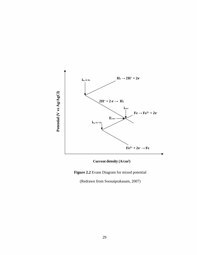
called the mixed or corrosion potential (Ecorr). The concept of mixed potential for iron

dissolution in deaerated hydrochloric acid is shown in Figure 2.2. The reduction process

need not be as simple as in the considered case but can be more complicated, involving

more than one reaction in addition to hydrogen evolution, such as oxygen reduction in the

case of aerated solutions [Fontana, 1986].

2.1.4 Free energy - electrode potential relationship

The change in free energy associated with an electrochemical reaction can be

expressed in terms of potential by the following expression:

∆G = − nFE (2.6)

where n is the number of electrons per atom of the species involved in the reaction, F is

the charge of 1 mol of electrons (96480 C/mol), and E is the electrode reduction

potential. As a convention, positive potential is associated with the spontaneous reaction

and, hence, the negative sign is used in Equation (2.6).

2.2 Kinetics of corrosion

Thermodynamics can provide a framework of possibility for different corrosion

reactions to occur. However, only based on kinetics, it is possible to elucidate those

reactions that will primarily occur and the rate at which they occur among the reactions

that are thermodynamically possible. For example, aluminum displays a predicative

thermodynamic tendency to react but is limited by its slow kinetics, which renders it

more resistant than other metals that are innately less reactive in certain environments.

29

Figure 2.2 Evans Diagram for mixed potential

(Redrawn from Soosaiprakasam, 2007)

H2 → 2H+ + 2e-

2H+ + 2 e- → H2

io, H+/H2

icorr

Ecorr

Fe → Fe2+ + 2e-

Fe2+ + 2e- → Fe

io, Fe2+/Fe

Current density (A/cm2)

Pote

nti

al (V

vs

Ag/A

gC

l)

30

2.2.1 Faraday’s law

A metal undergoing corrosion can be viewed as analogous to a short circuited

energy-producing electrochemical cell wherein the energy is produced by consumption of

reactants to form corrosion products. To be consistent with the principle of conservation

of mass, the amount of corrosion products formed has to be equal to the amount of the

reactants consumed. Also, for an electrochemical reaction, the electrons liberated by

anodic reaction have to be consumed by the cathodic reaction at the same rate, which

makes it possible to express corrosion in terms of electrochemical current. Hence, it can

be stated that the current flowing from an anodic reaction will be equal and opposite to

the current flowing into the cathodic reaction. This current can be used as an indicator of

rate of corrosion and can be correlated to the amount of material corroded by Faraday’s

law.

nF

Itam (2.7)

where m is the weight of the metal corroded (g), I is the current passed (A), t is time (s), a

is the atomic weight of the metal (g/mol), n is the number of electrons transferred, and F

is the charge per mole of electron. If multiple cathodic and anodic reactions can take

place, the corrosion current represents the sum of component partial currents. Also,

though, the anodic and cathodic currents have to be equal in magnitude, the

corresponding anodic and cathodic areas need not be equal. Hence, the respective current

density, which is clearly a function of the surface area of the corroding metal, can be

different. So when the anodic area of the corroding metal is almost equal to the cathodic

area, the corrosion is uniform. However, when the anodic area of the corroding metal is

31

relatively much smaller than the cathodic area, the nature of the corrosion will be

localized [ASM Handbook (13a), 1987].

Dividing Equation (2.7) by the surface area of the corroding metal (Ae) and

rearranging the yields, the following correlation is found between corrosion rate and

current density:

Corrosion rate (CR) = nF

ai

tA

m corr

e

(2.8)

where icorr

eA

Irepresents the corrosion current density.

2.2.2 Polarization

Even though corrosion is seldom an equilibrium process, it is essential to

understand the equilibrium state properties in order to analyze its non-equilibrium

behaviour. For any reaction at equilibrium, the rate of forward reaction is equal to the rate

of reverse reaction, and as a consequence, there is no net reaction but only an exchange

reaction rate. Exchange reaction rate can be readily expressed using exchange current

density (io), which can be defined as the current density at equilibrium corresponding to

the equal forward and reverse reactions at the electrode. For example, consider the

reversible hydrogen evolution reaction:

2H+ + 2e H2 (2.9)

For this reaction, the correlation between exchange reaction rate and current

density can be deduced from Faraday’s law:

nF

airr o

redoxid (2.10)

32

where io is the exchange current density and roxid and rred are the oxidation and reduction

rates at equilibrium, respectively.

A characteristic feature of io is its dependency on the nature of the surface

antithetical to the thermodynamic parameter, the potential. Thus, when a net current is

involved in an electrode process, the equilibrium is disturbed and causes a potential

change that is dependent on the direction and magnitude of the current. This potential

change, as a result of a net current, is called polarization and can be measured in volts.

The concept of polarization can be better understood by illustration using an

electrochemical cell (Daniell cell) as depicted in Figure 2.3a.

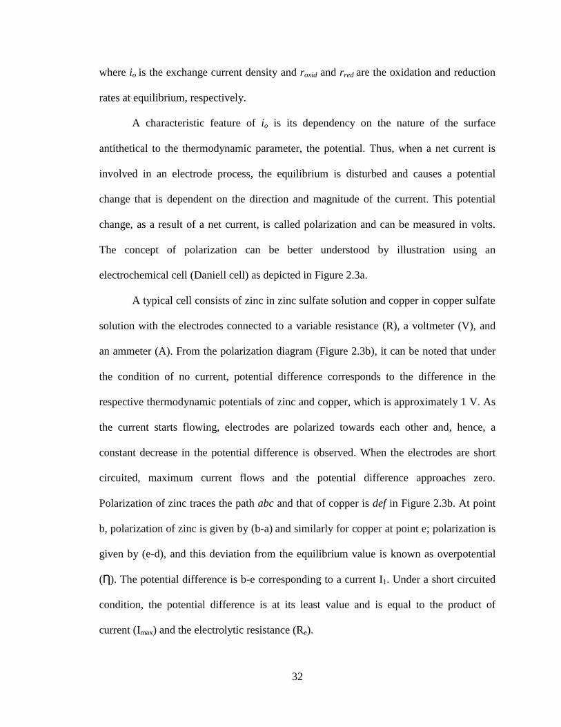
A typical cell consists of zinc in zinc sulfate solution and copper in copper sulfate

solution with the electrodes connected to a variable resistance (R), a voltmeter (V), and

an ammeter (A). From the polarization diagram (Figure 2.3b), it can be noted that under

the condition of no current, potential difference corresponds to the difference in the

respective thermodynamic potentials of zinc and copper, which is approximately 1 V. As

the current starts flowing, electrodes are polarized towards each other and, hence, a

constant decrease in the potential difference is observed. When the electrodes are short

circuited, maximum current flows and the potential difference approaches zero.

Polarization of zinc traces the path abc and that of copper is def in Figure 2.3b. At point

b, polarization of zinc is given by (b-a) and similarly for copper at point e; polarization is

given by (e-d), and this deviation from the equilibrium value is known as overpotential

(Ƞ). The potential difference is b-e corresponding to a current I1. Under a short circuited

condition, the potential difference is at its least value and is equal to the product of

current (Imax) and the electrolytic resistance (Re).

33

(a)

(b)

Figure 2.3 A typical electrochemical cell (Redrawn from Revie and Uhlig, 2008)

(a) Daniell Cell (b) Polarization behaviour of Daniell cell

V

A

Cu Zn

R

CuSO4 ZnSO4

log current

Po

ten

tia

l

φcorr

φCu

φZn

Imax Re

d

e

f

c

b

I1

a

Imax

34

Imax is indicative of the equivalent deposition rate of copper and, more importantly, the

equivalent corrosion rate for Zinc. As illustrated above, the corrosion process is

analogous to a short circuited electrolytic cell where the current Imax is given as the

corrosion current, Icorr, and the measured potential is given as the corrosion potential,

Ecorr, which represents the mixed potential of polarized anodes and cathodes. For

corrosion studies, alternatively, an external source can be used to polarize the metal

surface either in the anodic or cathodic direction, and the response of the system can be

evaluated. Cathodic polarization is characterized by the supply of electrons to the metal

rendering the metal negative in potential with respect to its equilibrium potential.

Conversely, for anodic polarization, electrons are withdrawn from the metal resulting in

an electron deficiency and, thereby, shifting the surface potential towards more positive

values [Revie and Uhlig, 2008]. Polarization can be sorted into three types based upon its

causes, and these are, namely, activation, concentration, and combined polarization.

2.2.2.1 Activation polarization

When one of the reactions occurring at the interface controls the net rate of an

electrochemical process, then the reaction is said to be under activation polarization. For

example, the hydrogen evolution reaction occurring on the metal surface in Equation

(2.3), in a simplest case scenario, can involve a number of steps such as adsorption of H+

ions onto the surface followed by electron transfer resulting in reduction of H+ to H, and,

finally, the hydrogen atoms coalescing to form a bubble of hydrogen gas. If one of the

above steps is the slowest and, hence, the rate determining step, then the system is

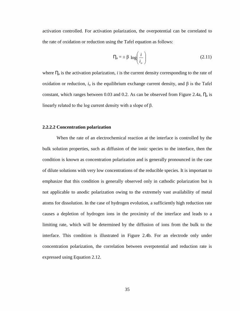
35

activation controlled. For activation polarization, the overpotential can be correlated to

the rate of oxidation or reduction using the Tafel equation as follows:

Ƞa = ± β

oi

ilog (2.11)

where Ƞa is the activation polarization, i is the current density corresponding to the rate of

oxidation or reduction, io is the equilibrium exchange current density, and β is the Tafel

constant, which ranges between 0.03 and 0.2. As can be observed from Figure 2.4a, Ƞa is

linearly related to the log current density with a slope of β.

2.2.2.2 Concentration polarization

When the rate of an electrochemical reaction at the interface is controlled by the

bulk solution properties, such as diffusion of the ionic species to the interface, then the

condition is known as concentration polarization and is generally pronounced in the case

of dilute solutions with very low concentrations of the reducible species. It is important to

emphasize that this condition is generally observed only in cathodic polarization but is

not applicable to anodic polarization owing to the extremely vast availability of metal

atoms for dissolution. In the case of hydrogen evolution, a sufficiently high reduction rate

causes a depletion of hydrogen ions in the proximity of the interface and leads to a

limiting rate, which will be determined by the diffusion of ions from the bulk to the

interface. This condition is illustrated in Figure 2.4b. For an electrode only under

concentration polarization, the correlation between overpotential and reduction rate is

expressed using Equation 2.12.

36

(a)

(b)

(c)

Figure 2.4 Types of polarization (a) Activation polarization (b) Concentration

polarization (c) Combined polarization

-0.3

-0.2

-0.1

0

0.1

0.2

0.001 0.01 0.1 1 10 100

-0.3

-0.2

-0.1

0

0.1

0.2

0.001 0.01 0.1 1 10 100

io,H2/H+

log i

Po

lari

zati

on

,Ƞ (

V)

Anodic slope = βa

Cathodic slope = βc

Acti

ve

No

ble

H2 → 2H+ + 2e-

2H+ + 2 e- → H2

0

iL

log i

(+)

(-)

Ƞco

nc

0

io

log i

(+)

(-)

Po

ten

tial

Ƞconc

ȠactȠT = Ƞa + Ƞc

37

Ƞc =

Li

i

nF

RT1log3.2 (2.12)

where Ƞc is the concentration polarization, i is the current density corresponding to the

rate of reduction, and Li is the limiting diffusion current density, which can be expressed

as a function of concentration of the reacting ions (CB) as follows:

x

nFCDi Bi

L (2.13)

where Di is the diffusion coefficient of the reacting ions and x is the thickness of the

diffusion layer. Environmental variables such as solution velocity, concentration, and

temperature are directly related to the limiting diffusion current density and, hence, the

net reaction rate [Fontana, 1986].

2.2.2.3 Combined polarization

Usually the combination of activation and concentration polarization is likely to

occur at an electrode where, at low reaction rates, the system is under activation

polarization and at higher rates, concentration polarization takes control. Hence, the total

polarization of the system can be expressed as follows:

ȠT = Ƞa + Ƞc (2.14)

Figure 2.4c represents the combined polarization curve. For anodic dissolution, Ƞc

can be eliminated for the reasons mentioned earlier, and, hence, the correlation between

the overpotential and current can be expressed as follows:

Ƞdiss = β

oi

ilog (2.15)

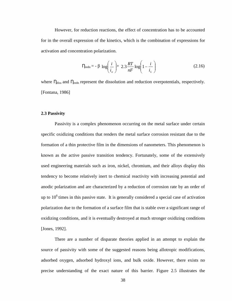
38

However, for reduction reactions, the effect of concentration has to be accounted

for in the overall expression of the kinetics, which is the combination of expressions for

activation and concentration polarization.

Ƞredn = - β

oi

ilog +

Li

i

nF

RT1log3.2 (2.16)

where Ƞdiss and Ƞredn represent the dissolution and reduction overpotentials, respectively.

[Fontana, 1986]

2.3 Passivity

Passivity is a complex phenomenon occurring on the metal surface under certain

specific oxidizing conditions that renders the metal surface corrosion resistant due to the

formation of a thin protective film in the dimensions of nanometers. This phenomenon is

known as the active passive transition tendency. Fortunately, some of the extensively

used engineering materials such as iron, nickel, chromium, and their alloys display this

tendency to become relatively inert to chemical reactivity with increasing potential and

anodic polarization and are characterized by a reduction of corrosion rate by an order of

up to 106

times in this passive state. It is generally considered a special case of activation

polarization due to the formation of a surface film that is stable over a significant range of

oxidizing conditions, and it is eventually destroyed at much stronger oxidizing conditions

[Jones, 1992].

There are a number of disparate theories applied in an attempt to explain the

source of passivity with some of the suggested reasons being allotropic modifications,

adsorbed oxygen, adsorbed hydroxyl ions, and bulk oxide. However, there exists no

precise understanding of the exact nature of this barrier. Figure 2.5 illustrates the

39

corrosion current density of an active passive metal as a function of potential. At low

values, corrosion rate increases with the potential until primary passivation potential (Epp)

is reached, beyond which the passive film is stabilized and the corrosion current density

is reduced to a lower value of ipass and remains almost constant. At much higher potential

(Eb), the passive film yields a transpassive state, and the current density increases again

with the potential. Environmental parameters such as solution velocity and oxidizer

concentration can either increase or not affect the corrosion rate, depending on the nature

of the metal and environment, and are generally complex in nature. An increase in

temperature, however, has been reported to increase the corrosion rate [Fontana, 1986].

2.4 Corrosion characterization techniques

2.4.1 Tafel extrapolation

Corrosion rate determination using Tafel extrapolation was initially carried out to

corroborate the validity of the mixed potential theory using the cathodic and anodic

polarization data [Fontana, 1986]. It was shown earlier, in Equation (2.11), that the

overpotential is linearly related to the logarithmic value of corrosion current density.

However, when a current is applied externally, such as, for example, cathodic current in

the case of cathodic polarization studies, at low values of current, the polarization curve

is non-linear due to the presence of a finite anodic current. However, at higher values of

current, the curve becomes linear as the corresponding anodic current is negligible, and

the opposite is observed during the measurement of anodic polarization. In actual

experiments, the polarization curve becomes linear at approximately 50 mV more active

or noble than the corrosion potential.

40

Figure 2.5 Active-passive transition behaviour of a metal (Redrawn from Jones, 1992)

Current density (A/cm2)

Active

Passive

Transpassive

icritipass

Eb

Epp

Ecorr

Po

ten

tial

(V

)

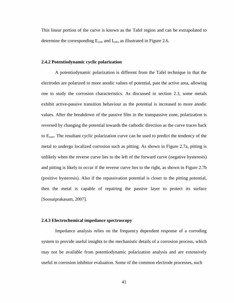
41

This linear portion of the curve is known as the Tafel region and can be extrapolated to

determine the corresponding Ecorr and Icorr, as illustrated in Figure 2.6.

2.4.2 Potentiodynamic cyclic polarization

A potentiodynamic polarization is different from the Tafel technique in that the

electrodes are polarized to more anodic values of potential, past the active area, allowing

one to study the corrosion characteristics. As discussed in section 2.3, some metals

exhibit active-passive transition behaviour as the potential is increased to more anodic

values. After the breakdown of the passive film in the transpassive zone, polarization is

reversed by changing the potential towards the cathodic direction as the curve traces back

to Ecorr. The resultant cyclic polarization curve can be used to predict the tendency of the

metal to undergo localized corrosion such as pitting. As shown in Figure 2.7a, pitting is

unlikely when the reverse curve lies to the left of the forward curve (negative hysteresis)

and pitting is likely to occur if the reverse curve lies to the right, as shown in Figure 2.7b

(positive hysteresis). Also if the repassivation potential is closer to the pitting potential,

then the metal is capable of repairing the passive layer to protect its surface

[Soosaiprakasam, 2007].

2.4.3 Electrochemical impedance spectroscopy

Impedance analysis relies on the frequency dependent response of a corroding

system to provide useful insights to the mechanistic details of a corrosion process, which

may not be available from potentiodynamic polarization analysis and are extensively

useful in corrosion inhibitor evaluation. Some of the common electrode processes, such

42

Figure 2.6 A typical Tafel plot (Redrawn from Srinivasan, 2006)

Ecorr

Icorr

Log current density

Pote

nti

al Anodic

Cathodic

43

(a)

(b)

Figure 2.7 A typical potentiodynamic cyclic polarization curve

(a) No pitting (b) Pitting

log i (A/cm2)

Active

Passive

Transpassive

icritipass

Eb

Epp

Ecorr

Epass

Erp

Negative

Po

ten

tial

(V

)

log i (A/cm2)

Active

Passive

Transpassive

icritipass

Eb

Epp

Ecorr

Epass

Erp

Positive

Po

ten

tial

(V

vs

Ag

/Ag

Cl)

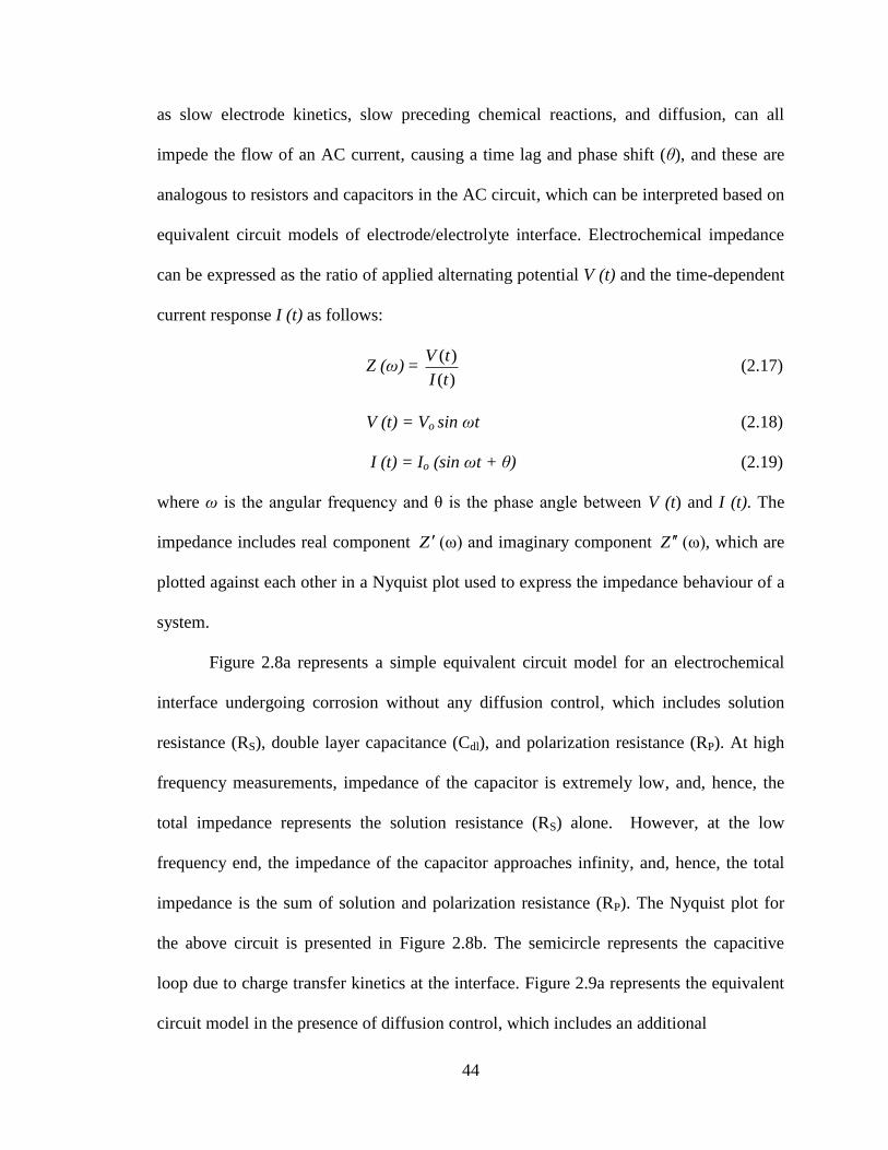
44

as slow electrode kinetics, slow preceding chemical reactions, and diffusion, can all

impede the flow of an AC current, causing a time lag and phase shift (θ), and these are

analogous to resistors and capacitors in the AC circuit, which can be interpreted based on

equivalent circuit models of electrode/electrolyte interface. Electrochemical impedance

can be expressed as the ratio of applied alternating potential V (t) and the time-dependent

current response I (t) as follows:

Z (ω) = )(

)(

tI

tV (2.17)

V (t) = Vo sin ωt (2.18)

I (t) = Io (sin ωt + θ) (2.19)

where ω is the angular frequency and θ is the phase angle between V (t) and I (t). The

impedance includes real component Z (ω) and imaginary component Z (ω), which are

plotted against each other in a Nyquist plot used to express the impedance behaviour of a

system.

Figure 2.8a represents a simple equivalent circuit model for an electrochemical

interface undergoing corrosion without any diffusion control, which includes solution

resistance (RS), double layer capacitance (Cdl), and polarization resistance (RP). At high

frequency measurements, impedance of the capacitor is extremely low, and, hence, the

total impedance represents the solution resistance (RS) alone. However, at the low

frequency end, the impedance of the capacitor approaches infinity, and, hence, the total

impedance is the sum of solution and polarization resistance (RP). The Nyquist plot for

the above circuit is presented in Figure 2.8b. The semicircle represents the capacitive

loop due to charge transfer kinetics at the interface. Figure 2.9a represents the equivalent

circuit model in the presence of diffusion control, which includes an additional

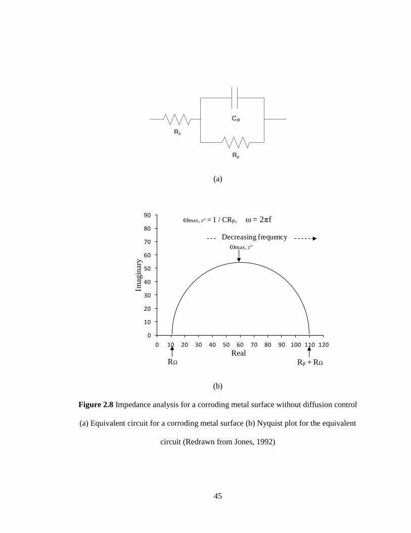
45

(a)

(b)

Figure 2.8 Impedance analysis for a corroding metal surface without diffusion control

(a) Equivalent circuit for a corroding metal surface (b) Nyquist plot for the equivalent

circuit (Redrawn from Jones, 1992)

Rp

Cdl

Rs

0

10

20

30

40

50

60

70

80

90

0 10 20 30 40 50 60 70 80 90 100 110 120

0

10

20

30

40

50

60

70

80

90

0 10 20 30 40 50 60 70 80 90 100 110 120

RΩ Rp + RΩ

Real

Imag

inar

y

Decreasing frequency

ωmax, Z'''

ωmax, Z''' = 1 / CRp, ω = 2πf

46

(a)

(b)

Figure 2.9 Impedance analysis for a corroding metal surface with diffusion control

(a) Equivalent circuit for a corroding metal surface (b) Nyquist plot for the equivalent

circuit (Redrawn from Jones, 1992)

Rp

Cdl

Rs

W

Rp

Rs

Cdl

Real

Imag

inar

y

0

10

20

30

40

50

60

70

80

90

0 10 20 30 40 50 60 70 80 90 100 110 120

0

10

20

30

40

50

60

70

80

90

0 10 20 30 40 50 60 70 80 90 100 110 120

Decreasing frequency

47

component of resistance in series with the polarization resistance, called Warburg

impedance. The low frequency end of the Nyquist plot is characterized by linearity

(diffusion tail) as shown in Figure 2.9b. This condition is frequently observed when a

surface film is formed over the metal surface, which limits the diffusion of corrosive

species across the interface.

Despite the advantages of the EIS techniques, it has some drawbacks such as the

complexity and ambiguity in the data interpretation at low frequency measurements

where it tends to approach the DC measurements. Nevertheless, impedance analysis can

provide some unique mechanistic information that cannot be obtained using DC

techniques.

2.5 Corrosion control techniques – Corrosion inhibitors

Corrosion inhibitors are chemicals that are capable of reacting either with the

metallic surface or the environment and reduce corrosion. Usage of corrosion inhibitors

has been one of the commonly employed methods to mitigate corrosion, and, hence, a

myriad of compounds have been reported to act as corrosion inhibitors by different

mechanisms. Corrosion inhibitors usually function by either increasing anodic or

cathodic polarization behaviour, by restricting the movement of ions to the metal surface,

or by increasing the electrical resistance of the surface to be protected. They can be

classified based on their mechanism, chemistry, or application. The most common

approach to classifying inhibitors is by their mechanism, and, as such, they can be

categorized as anodic, cathodic, and film forming inhibitors.

48

2.5.1 Anodic inhibitors

Anodic inhibitors or passivators are the most effective and commonly used type,

and they function by shifting the corrosion potential to more anodic values, as shown in

Figure 2.10a. This forces the metal to its passive region. They can either contain

oxidizing ions such as chromate or nitrite that can effectively passivate steel even without

the presence of oxygen, or they can contain non-oxidizing ions such as phosphate or

molybdate that can also passivate steel but only in the presence of oxygen. The

concentration of the inhibitor is a critical factor since a deficiency can cause localized

pitting corrosion. Hence, it is important to monitor the concentration of the inhibitor on a

regular basis.

2.5.2 Cathodic inhibitors

Cathodic inhibitors typically interfere with the cathodic reactions of corrosion by

either directly slowing down the reaction or by formation of surface deposits that limit

the diffusion. They are generally characterized by shifting the corrosion potential to more

cathodic values, as depicted in Figure 2.10b, and are considered safer than anodic

inhibitors as they do not pose risks of pitting corrosion. They can function by three

different mechanisms, namely, cathodic poisoning, precipitation, and oxygen scavenging.

Inhibitors based on arsenic and antimony function by making the recombination and

discharge of hydrogen difficult, thereby reducing the rate of cathodic reaction and, hence,

the net corrosion rate. Inhibitors based on zinc and calcium function by precipitating in

the form of oxides on the metal surface. Finally, oxygen scavengers such as sulfite and

bisulfite ions function by specifically reacting with oxygen.

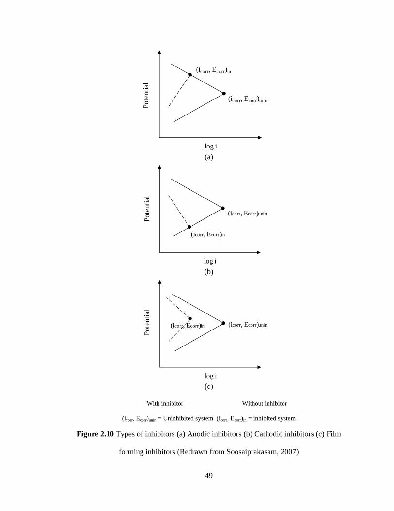
49

(a)

(b)

(c)

With inhibitor Without inhibitor

(icorr, Ecorr)unin = Uninhibited system (icorr, Ecorr)in = inhibited system

Figure 2.10 Types of inhibitors (a) Anodic inhibitors (b) Cathodic inhibitors (c) Film

forming inhibitors (Redrawn from Soosaiprakasam, 2007)

log iP

ote

nti

al

(icorr, Ecorr)unin

(icorr, Ecorr)in

log i

Pote

nti

al

(icorr, Ecorr)unin

(icorr, Ecorr)in

log i

Po

ten

tial

(icorr, Ecorr)unin(icorr, Ecorr)in

50

2.5.3 Film forming inhibitors

This category of inhibitors is primarily constituted by organic compounds that are

capable of forming a hydrophobic film on the corroding metal surface that can act as a

physical barrier. When present in adequate levels of concentration, they tend to interact

with the entire metal surface and both anodic and cathodic effects might be observed as

shown in Figure 2.10c. Film formation is clearly based on adsorption, and, consequently,

the environmental parameters such as temperature and pressure can be critical. Chemical

composition, molecular structure, and the strength of the adsorption bond formed with the

metal surface are some of the factors that can influence the effectiveness of an organic

inhibitor. They can either be cationic in nature, such as amines, or anionic as in the case

of sulfolane, and depending on the residual charge of the metal, they will be adsorbed

[NACE1, 2012]. Generally, when organic inhibitors are introduced in a corroding system,

they alter the properties of the double layer by adsorbing at the metal-solution interface,

and the reaction can be summarized as follows:

M (nH2O) ads + I(s) MIads + nH2O (2.20)

Corrosion inhibitor molecules present in the solution displace the water molecules

adsorbed on the metal surface and are preferentially adsorbed.

2.6 Selection of corrosion inhibitors

In the process of development of a corrosion inhibitor, selection of appropriate

chemical compounds is the most crucial step. The selection of inhibitors has mostly been

empirical and based on the macroscopic understanding of physico-chemical properties

only. However, many recent works emphasize the importance of understanding the

51

compounds at a molecular level to comprehend their inhibition properties [Öğretir et al

(1999); Sastri and Perumareddi (1997)]. This assumes specific importance because

corrosion inhibition is generally considered to involve electron transfer between the

inhibitor and the metal in either direction. Consequently, factors such as availability of π

electrons due to the presence of unsaturated bonds, as in aromatic compounds and the

presence of reactive functional groups with the ability to donate electrons, which are

considered to facilitate electron transfer from the inhibitor to the metal. Properties of the

donor atom of the functional group, such as electron density and polarizability, can also

influence the inhibition characteristics of the inhibitor. Hence, it is an enhanced

understanding of the properties of the chemical compounds at a molecular level is

essential, in addition to general empirical knowledge, to render the selection process

more scientific.

The hard and soft acids and bases (HSAB) principle is a tool that can be

extensively useful in the process of design and selection of a corrosion inhibitor [Sastri,

2001]. As per the HSAB principle, every chemical compound can be classified into a

hard, soft, or borderline category of acid or base depending upon the compund’s

molecular parameters such as electronegativity, polarizability, size, and hardness

(calculated from ionization potential and electron affinity). For instance, when the

polarizability of a compound is low, it signifies hard characteristics, and higher values

signify soft characteristics, whereas the converse is true for electronegativity. Also

according to HSAB theory, homogenous interactions among the species are greatly

favoured, which implies that hard acids tend to form complexes with hard bases, whereas

soft acids tend to form complexes with soft bases and borderline bases can interact with

52

both soft and hard bases. Thus, it is important to classify the metal to be protected based

on the HSAB principle so that the potential corrosion inhibitors can be chosen

accordingly.

2.7 Quantum chemical analysis of corrosion inhibitors

Quantum chemical methods for corrosion inhibition studies, though they cannot

be used to directly predict corrosion in an absolute sense, can still be used to obtain

useful qualitative to semi-quantitative information to understand the corrosion inhibition

process. Generally, corrosion inhibition studies from a quantum chemical perspective

cannot be rigorously achieved due to the numerous parameters associated with the

process and the enormously complex interaction between them [Öğretir et al., 1999].

Some of the commonly reported quantum chemical indices that are correlated with

inhibition efficiencies are Highest occupied molecular orbital energy (EHOMO), Energy

gap (∆E) between highest occupied molecular orbital energy and lowest unoccupied

molecular orbital energy (EHOMO - ELUMO), Dipole moment (µ), and Charge on the donor

atom (Z) [Chakrabarti (1984); Sastri (2001); Khalil (2003); Öğretir et al (1999)]. EHOMO

is associated with the electron donating ability of a molecule, and, hence, higher values

indicate better inhibition efficiency. Similarly, ELUMO represents the ability of a molecule

to accept electrons, and, consequently, lower values of ∆E can cause higher inhibition

efficiency. For µ, lower values will favour accumulation of inhibitor in the surface layer,

leading to better inhibition, and in case of Z, the higher the value, the better the corrosion

inhibition [Khaled and Hackerman, 2003]. In some works, the fraction of electrons (∆N)

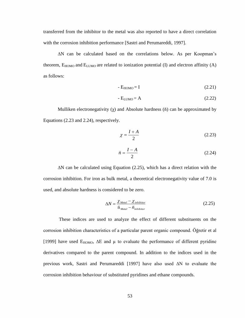
53

transferred from the inhibitor to the metal was also reported to have a direct correlation

with the corrosion inhibition performance [Sastri and Perumareddi, 1997].

∆N can be calculated based on the correlations below. As per Koopman’s

theorem, EHOMO and ELUMO are related to ionization potential (I) and electron affinity (A)

as follows:

- EHOMO = I (2.21)

- ELUMO = A (2.22)

Mulliken electronegativity (χ) and Absolute hardness (ň) can be approximated by

Equations (2.23 and 2.24), respectively.

2

AI (2.23)

2

AIn

(2.24)

∆N can be calculated using Equation (2.25), which has a direct relation with the

corrosion inhibition. For iron as bulk metal, a theoretical electronegativity value of 7.0 is

used, and absolute hardness is considered to be zero.

inhibitorMetal

inhibitorMetal

nN

n

(2.25)

These indices are used to analyze the effect of different substituents on the

corrosion inhibition characteristics of a particular parent organic compound. Öğretir et al

[1999] have used EHOMO, ∆E and µ to evaluate the performance of different pyridine

derivatives compared to the parent compound. In addition to the indices used in the

previous work, Sastri and Perumareddi [1997] have also used ∆N to evaluate the

corrosion inhibition behaviour of substituted pyridines and ethane compounds.

54

In another work by the same authors EHOMO, ∆E and charge on the nitrogen atom

(Zn) were correlated with the corrosion inhibition performance [Sastri and Perumareddi,

1994].

55

3. SELECTION AND TESTING OF CORROSION INHIBITORS

3.1 Selection of tested corrosion inhibitors

3.1.1 Selection of compounds

The principle of hard and soft acids and bases (HSAB) was used for theoretical

selection of corrosion inhibitors to be tested. For the case of amine-based CO2 absorption

processes, the most commonly used material of construction is carbon steel and the

general corrosion products was reported to be iron carbonate (FeCO3) [Kohl and Nielson,

1997, Hamah-Ali et al, 2011]. In FeCO3, iron is in a divalent (Fe2+

) state, which is

classified as a borderline acid [Sastri, 2001]. Therefore, the preferred choice of inhibitor

must possess borderline basic characteristics in order to best protect carbon steel

predominantly in a divalent oxidation state.

Also based on the general empirical understanding of organic compounds used as

corrosion inhibitors, sulfur-containing compounds were reported to be more effective due

to their better electron donating ability than nitrogen or oxygen [Sastri (2001);

Hackerman and Makrides (1954); Khaled and Hackerman (2003)]. Theoretical and

empirical considerations, as illustrated above, were used in the selection of inhibitors.

A total of thirteen compounds were chosen in which ten compounds were selected

based on the HSAB principle, including aniline- and pyridine-based compounds, and the

other three compounds were based on general empirical considerations. The list of

compounds chosen is presented in Table 3.1. Broadly, the selected inhibitors can be

sorted into three categories, namely, aniline-based, pyridine-based, and other compounds.

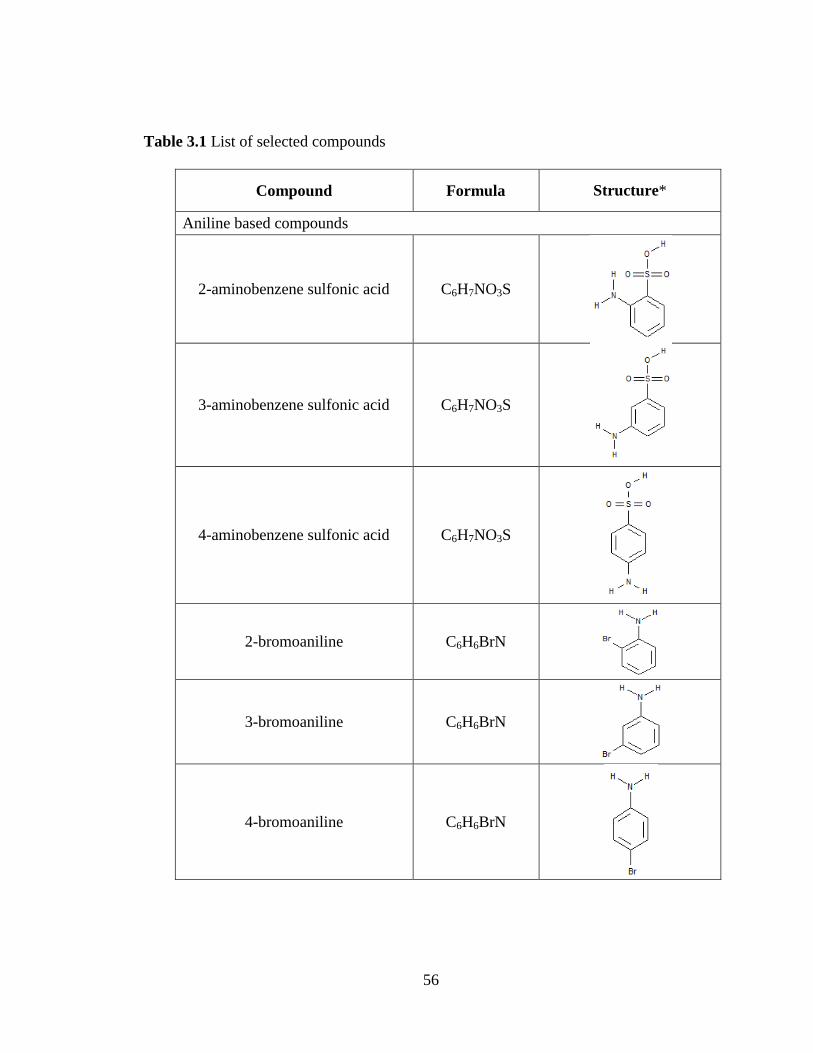
56

Table 3.1 List of selected compounds

Compound Formula Structure*

Aniline based compounds

2-aminobenzene sulfonic acid C6H7NO3S



2-bromoaniline C6H6BrN



57

Table 3.1 List of selected compounds (continued)

Compound Formula Structure*

Sulfapyridine C11H11N3O2S

Sulfanilamide C6H8N2O2S

Pyridine based compounds

2-bromopyridine C5H4BrN

3-bromopyridine C5H4BrN

Other compounds

Sulfolane C4H8O2S

Thiosalicylic acid C7H6O2S

Sodium thiosulfate Na2S2O3

* Molecular structures redrawn from PubChem database [PubChem1]

58

Eight substituted compounds of aniline were chosen due to their borderline

characteristics that enable them to interact with the metal surface effectively. Ortho,

para, and meta substituted aminobenzene sulfonic acids contain a sulfur (S) and an

oxygen (O) donor atom in addition to a nitrogen (N) atom that can act as a reaction center

for adsorption. Similarly, ortho, para, and meta substituted bromoanilines were chosen

since the natural borderline characteristics of the aniline will be enhanced by a borderline

substituent Br-. Sulfanilamide is also a substituted compound of aniline with one S and

two N and O reaction centers. Sulfpyridine is a derivative of sulfanilamide with a

pyridine ring attached to the nitrogen atom.

Substituted pyridine compounds also display borderline characteristics besides

being reported as corrosion inhibitors and, hence, are ideal choices for corrosion

inhibitors, especially the bromine (Br-) substituted compounds such as 2-bromopyridine

and 3-bromopyridine where Br- can enhance the borderline characteristics.

Sulfolane, a heterocyclic compound with a sulfonyl reaction center and

thiosalicylic acid with one S and two O reaction centers were the other compounds

chosen. Sodium thiosulfate, a process contaminant in the amine-based CO2 absorption

process, when tested for its effect in the preliminary experiments, caused a drastic

reduction in corrosion rate. Hence, sodium thiosulfate was also tested along with other

organic inhibitors.

3.1.2 Toxicity evaluation

The preliminary selection was followed by a screening process that used the

values of toxicity of the compounds as the screening criteria. The specific criteria is that

59

the corrosion inhibitors must not be more toxic than the absorbents used in the CO2

capture process (i.e., their lethal dosage (LD50) values must be equal or greater than those

of the absorbents). Although DEA is the most toxic absorbent among those listed in

Table 3.2, the toxicity of MEA was set as the basis for screening inhibitors. This is

because MEA is the most prevalent benchmark solvent for absorbents used in carbon

capture applications. Thus, the cut-point toxicity is LD50 ORAL Rat < 1720 mg/kg.

Ecological information on the selected organic compounds is compiled in Table

3.3. It was not possible to obtain all the details of ecological information for all the

chemical compounds considered; however, based on the available details, it was possible

to eliminate certain compounds that are explicitly not safe and do not meet the screening

criteria. Generally, bromine compounds are considered suspected carcinogens, and

among the Br- substituted compounds selected, only the toxicity values of 4-bromoaniline

and 2-bromopyridine were available and neither met the screening criteria. It can also be

observed that in the material safety data sheets (MSDS) for these compounds, the

ecological properties of the parent compound and some of its derivatives for which the

data is available were considered representative of a whole group of compounds. In line

with that, the toxicity values of those compounds for which the data is available were

taken as a guideline for assessing compounds that are structural isomers of the same

compound.

Also, hazard rating for each compound was taken as a guideline to define the

toxicity of the material. Due to their toxicity and suspected carcinogenic nature, the five

Br- substituted compounds were eliminated from further analysis.

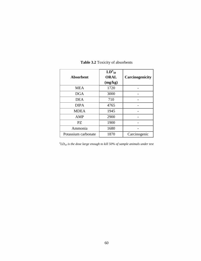
60

Table 3.2 Toxicity of absorbents

Absorbent

LDa

50

ORAL

(mg/kg)

Carcinogenicity

MEA 1720 -

DGA 3000 -

DEA 710 -

DIPA 4765 -

MDEA 1945 -

AMP 2900 -

PZ 1900 -

Ammonia 1680 -

Potassium carbonate 1870 Carcinogenic

aLD50 is the dose large enough to kill 50% of sample animals under test

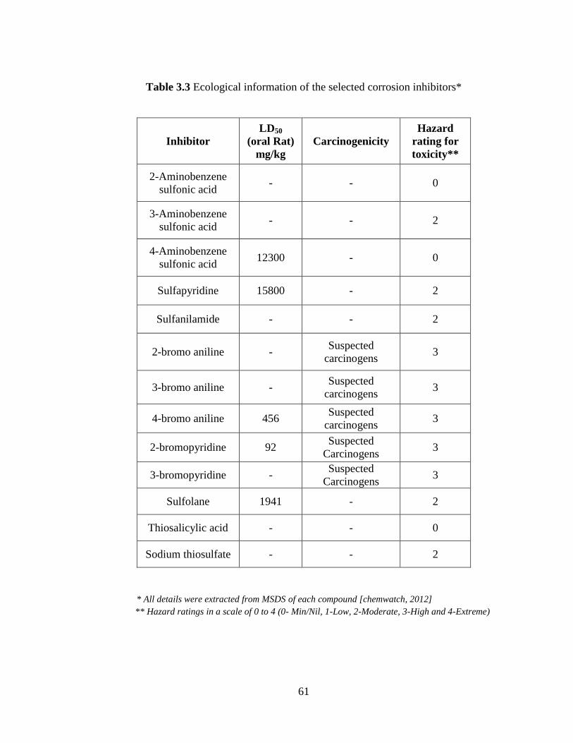
61

Table 3.3 Ecological information of the selected corrosion inhibitors*

Inhibitor

LD50

(oral Rat)

mg/kg

Carcinogenicity

Hazard

rating for

toxicity**

2-Aminobenzene

sulfonic acid - - 0

3-Aminobenzene

sulfonic acid - - 2

4-Aminobenzene

sulfonic acid 12300 - 0

Sulfapyridine 15800 - 2

Sulfanilamide - - 2

2-bromo aniline - Suspected

carcinogens 3

3-bromo aniline - Suspected

carcinogens 3

4-bromo aniline 456 Suspected

carcinogens 3

2-bromopyridine 92 Suspected

Carcinogens 3

3-bromopyridine - Suspected

Carcinogens 3

Sulfolane 1941 - 2

Thiosalicylic acid - - 0

Sodium thiosulfate - - 2

* All details were extracted from MSDS of each compound [chemwatch, 2012]

** Hazard ratings in a scale of 0 to 4 (0- Min/Nil, 1-Low, 2-Moderate, 3-High and 4-Extreme)

62

Only eight compounds were selected for further analysis, namely 2-aminobenzene

sulfonic acid, 3-aminobenzene sulfonic acid, 4-aminobenzene sulfonic acid,

sulfapyridine, sulfanilamide, sulfolane, thiosalicylic acid, and sodium thiosulfate.

3.1.3 Quantum chemical analysis

Quantum chemical analysis was carried out to determine the quantum chemical

parameters such as highest occupied molecular orbital energy (EHOMO), energy gap (∆E)

between highest occupied molecular orbital energy and lowest unoccupied molecular

orbital energy (EHOMO - ELUMO), dipole moment (µ), fraction of electron transferred (∆N),

and charge of the donor atom (Z). EHOMO, ∆N and Z have a direct relation with inhibition

efficiencies whereas ∆E and µ have an inverse relation [Chakrabarti (1984); Sastri

(2001); Khalil (2003); Khaled and Hackerman (2003); Sastri and Perumareddi (1997)].

Generally, these indices are used to analyze the effect of different substituents on

the corrosion inhibition characteristics of a particular parent organic compound.

However, for this study, of the eight compounds selected, only seven compounds were

organic. Among them, only five compounds were derivatives of one parent compound,

aniline, and, hence, could be evaluated comparatively. The quantum chemical parameters

for the other two compounds that were distinctly different from the rest were also

determined. The only commonality among all the selected organic compounds is the

presence of a sulfur atom that can act as the adsorption center. Hence, the charge of the

sulfur atom (Zs) and ∆N were used to compare all the compounds studied.

Semi-empirical quantum chemistry calculations package MOPAC2007 was used

to perform PM-6 (Parameterization) calculations from which the quantum chemical

63

parameters for selected corrosion inhibitors were obtained by specifying the molecular

geometry of each compound [PubChem1, 2011]. Values of EHOMO, ∆E, and µ can be

directly obtained from the software, whereas the values of ∆N and Zs were obtained by

further analysis and are presented in Table 3.4. Trends of different parameters are

presented in Figure 3.1.

In Figures 3.1a, 3.1b, and 3.1c, five aniline derivatives are compared, where

sulfapyridine has the highest EHOMO value and, hence, better than the other compounds.

However, in terms of ∆E and µ, 3-aminobenzene sulfonic acid and 2-aminobenzene

sulfonic acid were better than other compounds, respectively. In the case of ∆N and Zs

(Figures 3.1d and 3.1e), sulfapyridine was better than all the other compounds. From the

comparisons based on different parameters, 2-aminobenzene sulfonic acid, 3-

aminobenzene sulfonic acid, and sulfapyridine are potential corrosion inhibitors.

64

Table 3.4 Quantum chemical parameters for selected compounds

Compound EHOMO

(eV)

ΔE

(eV)

µ

(debye) ∆N Zs

2-aminobenzene sulfonic acid -9.17 8.61 4.64 0.25 2.54



Sulfanilamide -9.18 8.89 6.50 0.25 2.52

Sulfapyridine -9.01 8.78 7.96 0.27 2.56

thiosalicylic acid -9.27 7.82 2.73 0.21 -0.18

Sulfolane -10.82 2.44 5.88 0.18 2.44

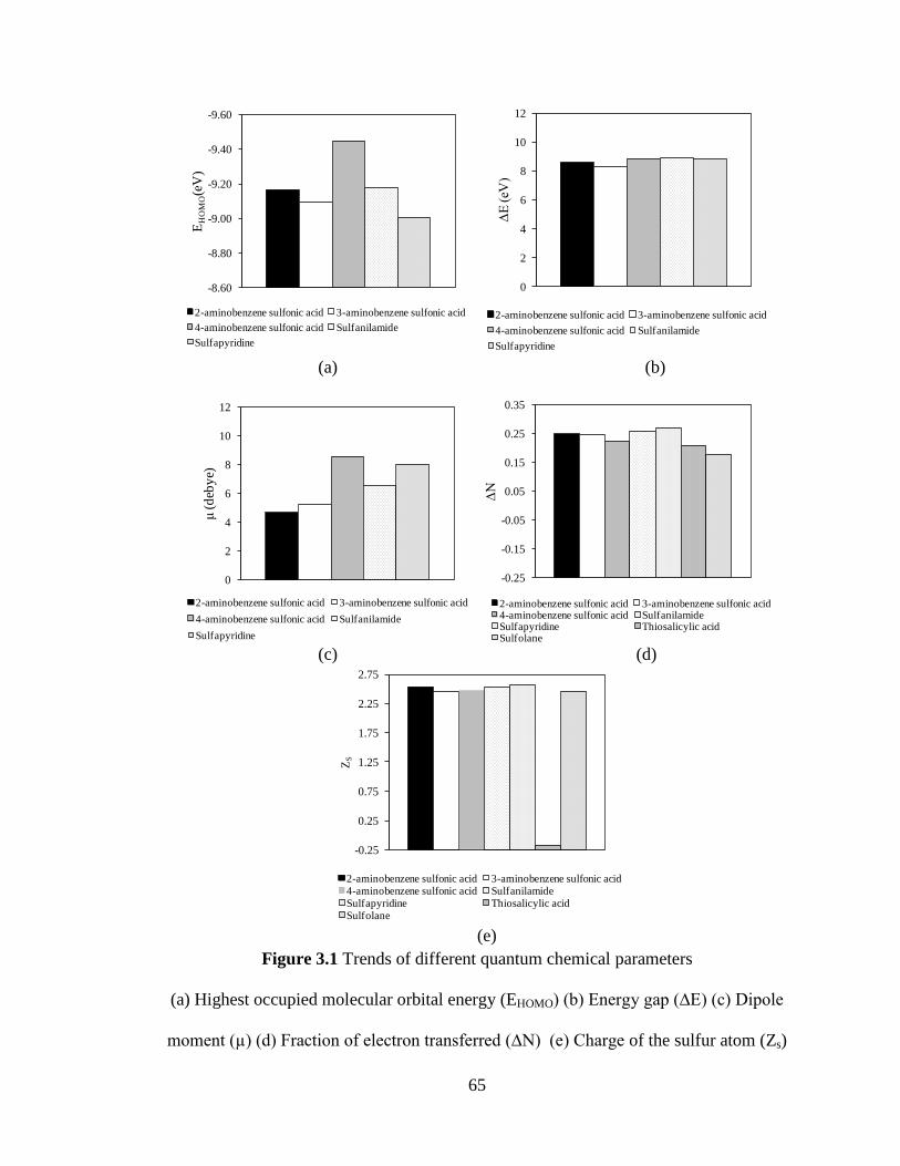
65

(a) (b)

(c) (d)

(e)

Figure 3.1 Trends of different quantum chemical parameters

(a) Highest occupied molecular orbital energy (EHOMO) (b) Energy gap (∆E) (c) Dipole

moment (µ) (d) Fraction of electron transferred (∆N) (e) Charge of the sulfur atom (Zs)

-9.60

-9.40

-9.20

-9.00

-8.80

-8.60

EH

OM

O(e

V)

2-aminobenzene sulfonic acid 3-aminobenzene sulfonic acid

4-aminobenzene sulfonic acid Sulfanilamide

Sulfapyridine

0

2

4

6

8

10

12

∆E

(eV

)



Sulfapyridine

0

2

4

6

8

10

12

μ(d

eby

e)



Sulfapyridine

-0.25

-0.15

-0.05

0.05

0.15

0.25

0.35

∆N

2-aminobenzene sulfonic acid 3-aminobenzene sulfonic acid4-aminobenzene sulfonic acid SulfanilamideSulfapyridine Thiosalicylic acidSulfolane

-0.25

0.25

0.75

1.25

1.75

2.25

2.75

ZS

2-aminobenzene sulfonic acid 3-aminobenzene sulfonic acid4-aminobenzene sulfonic acid SulfanilamideSulfapyridine Thiosalicylic acidSulfolane

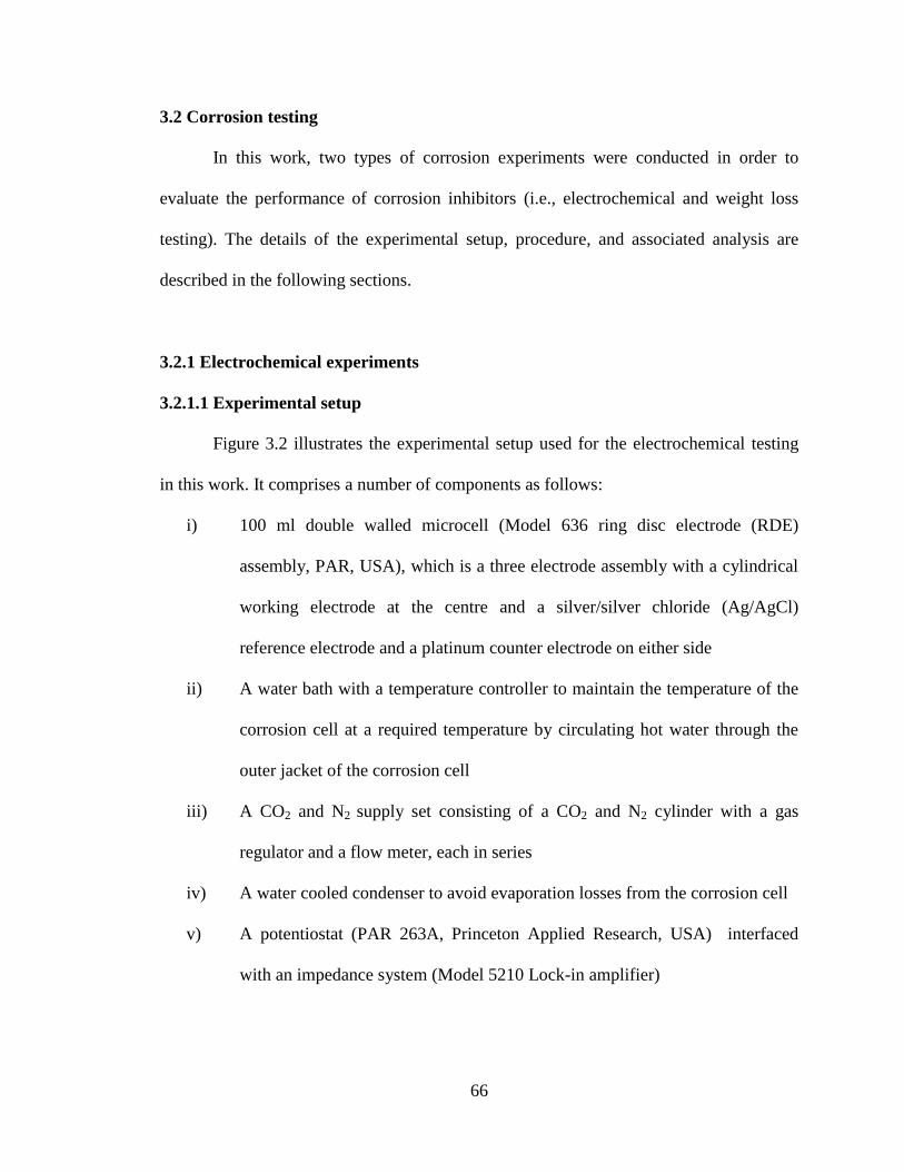
66

3.2 Corrosion testing

In this work, two types of corrosion experiments were conducted in order to

evaluate the performance of corrosion inhibitors (i.e., electrochemical and weight loss

testing). The details of the experimental setup, procedure, and associated analysis are

described in the following sections.

3.2.1 Electrochemical experiments

3.2.1.1 Experimental setup

Figure 3.2 illustrates the experimental setup used for the electrochemical testing

in this work. It comprises a number of components as follows:

i) 100 ml double walled microcell (Model 636 ring disc electrode (RDE)

assembly, PAR, USA), which is a three electrode assembly with a cylindrical

working electrode at the centre and a silver/silver chloride (Ag/AgCl)

reference electrode and a platinum counter electrode on either side

ii) A water bath with a temperature controller to maintain the temperature of the

corrosion cell at a required temperature by circulating hot water through the

outer jacket of the corrosion cell

iii) A CO2 and N2 supply set consisting of a CO2 and N2 cylinder with a gas

regulator and a flow meter, each in series

iv) A water cooled condenser to avoid evaporation losses from the corrosion cell

v) A potentiostat (PAR 263A, Princeton Applied Research, USA) interfaced

with an impedance system (Model 5210 Lock-in amplifier)

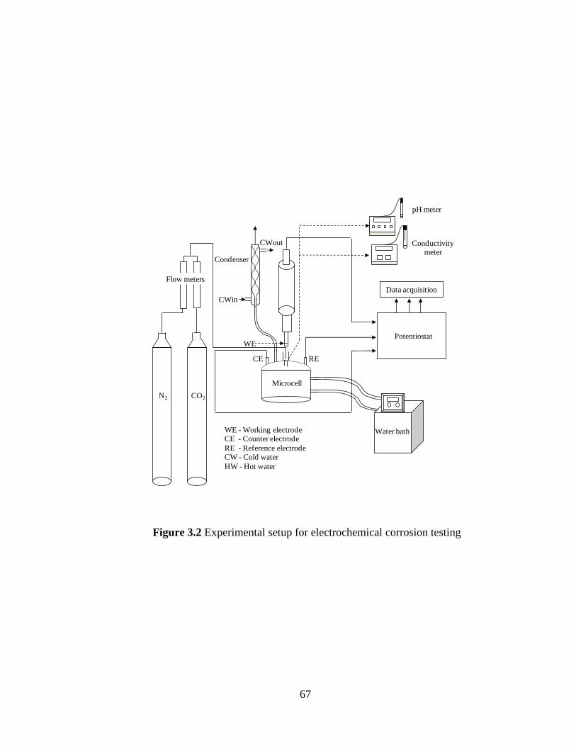
67

Figure 3.2 Experimental setup for electrochemical corrosion testing

Potentiostat

Data acquisition

N2 CO2

Flow meters

Condenser

CWin

WE - Working electrode CE - Counter electrode

RE - Reference electrode CW - Cold water

HW - Hot water

CE RE

CWout

WE

Conductivity meter

pH meter

Microcell

Water bath

68

vi) Powercorr (Version 2.53) software to record and analyze the results by

interfacing with a PC

vii) A pH meter (Oakton pH510 series)

viii) A conductivity meter (YSI 3200 conductivity instrument)

3.2.1.2 Specimen preparation

Carbon steel (CS 1018 with the composition of 0.175% carbon, 0.75%

manganese, and balance iron) was chosen as the working electrode (specimen) due to its

common use as construction material in amine-based CO2 capture plants [Dupart et al.,

1993]. The specimens were cylindrical with dimensions of 0.8 cm in height, 1.2 cm

outside diameter, and 0.6 cm central hole, as shown in Figure 3.3. The surface of each

specimen was prepared by wet grinding with 600 grit silicon carbide papers using

deionized water, being degreased with high purity methanol, rinsed with deionized water,

and then dried as per ASTM G1-90 (1999) before being introduced into the solution for

testing.

3.2.1.3 Solution preparation

Monoethanolamine (MEA) was chosen in this work as the absorption solvent

since it has been used as the benchmark in both demonstration and commercial CO2

capture plants. Its concentration was fixed at 5.0 kmol/m3 or 30% by weight to represent

the common strength of the service MEA solution in practice [Kohl and Nielson, 1997].

The aqueous solution of MEA was prepared from 99% reagent grade MEA and deionized

water.

69

Figure 3.3 A sketch of electrochemical testing specimens

0.6 cm

1.2 cm

0.8 cm

70

The solution was saturated with CO2 with a CO2 loading of 0.55±0.05 mol CO2 /

mol MEA. To these final solutions, a measured weight of tested corrosion inhibitor was

added. Inhibitor concentrations (250-10000 ppm) were chosen to be within the range of

the literature values (Table 1.2). The same procedure was repeated for different corrosion

inhibitors tested. In some tests, process contaminants, namely sodium chloride (NaCl)

and formic acid (CH2O2), with concentrations of 10,000 ppm were added to the test

solution for the study of process contaminant effects on the inhibitor performance. To

determine the MEA solution concentration, a measured volume of the solution sample

was titrated with hydrochloric acid (HCl) using methyl orange indicator. For every drop

of HCl added, a corresponding volume of CO2 was liberated. Its volume was measured

using a Chittick’s apparatus, which was attached to the titration setup (Figure 3.4). Based

on the volume of CO2 liberated, the CO2 loading of the solution was determined. A

summary of the chemicals used for the experiments are presented in Table 3.5.

3.2.1.4 Experimental procedure

The experiment began with charging the prepared MEA solution into the

corrosion cell. The corrosion cell was then fitted with a condenser to prevent evaporation

loss of the test solution, purged with gaseous CO2 to maintain the CO2 saturated loading

of the solution, and connected to a heater circulator to maintain the temperature of

solution at 80oC. After the solution temperature reached 80

oC, solution samples were

taken for analysis of MEA concentration and CO2 loading. The conductivity and pH of

the tested solution were directly measured from the corrosion cell. The corrosion cell was

assembled with a working electrode (specimen), a counter electrode, and a reference

71

Figure 3.4 Chittick’s apparatus for CO2 loading measurement

1 1

1 11

11

Burette (50 ml)

Sample

Conical Flask

Levelling bulb

Graduated gas measuring tube

Stopper

Glass T-tube

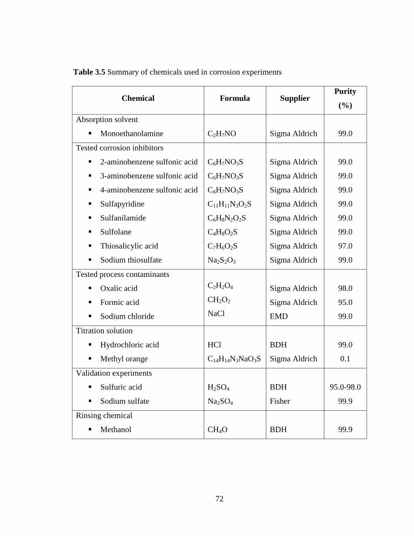
72

Table 3.5 Summary of chemicals used in corrosion experiments

Chemical Formula Supplier Purity

(%)

Absorption solvent

Monoethanolamine

C2H7NO

Sigma Aldrich

99.0

Tested corrosion inhibitors

2-aminobenzene sulfonic acid



Sulfapyridine

Sulfanilamide

Sulfolane

Thiosalicylic acid

Sodium thiosulfate

C6H7NO3S

C6H7NO3S

C6H7NO3S

C11H11N3O2S

C6H8N2O2S

C4H8O2S

C7H6O2S

Na2S2O3

Sigma Aldrich

Sigma Aldrich

Sigma Aldrich

Sigma Aldrich

Sigma Aldrich

Sigma Aldrich

Sigma Aldrich

Sigma Aldrich

99.0

99.0

99.0

99.0

99.0

99.0

97.0

99.0

Tested process contaminants

Oxalic acid

Formic acid

Sodium chloride

C2H2O4

CH2O2

NaCl

Sigma Aldrich

Sigma Aldrich

EMD

98.0

95.0

99.0

Titration solution

Hydrochloric acid

Methyl orange

HCl

C14H14N3NaO3S

BDH

Sigma Aldrich

99.0

0.1

Validation experiments

Sulfuric acid

Sodium sulfate

H2SO4

Na2SO4

BDH

Fisher

95.0-98.0

99.9

Rinsing chemical

Methanol

CH4O

BDH

99.9

73

electrode and then connected to the potentiostat. The open circuit potentials (OCP) were

recorded as a function of time until reaching a steady state value (±1 mV for 300

seconds). After the steady state OCP value was obtained, impedance analysis was carried

out. The AC amplitude of 10 mV was applied over a frequency range of 10 kHz to 10

mHz. The corresponding impedance values, resolved into imaginary and real

components, were measured as a function of frequency. Since the excitation potential was

a very small magnitude, there was a minimum system perturbation OCP and the system

returned to its steady state OCP in 5 to 10 minutes.

After the impedance measurement, cyclic potentiodynamic polarization scans

were carried out at a scan rate of 10 mV/min. On the completion of each experiment,

solution samples were taken again for measuring MEA concentration and CO2 loading of

solutions. The values of conductivity and pH of the solution were measured and recorded.

3.2.1.5 Validation of experimental setup

The experimental setup and procedure for potentiodynamic polarization was

validated using ASTM G5-94 (Reapproved 2004) preceding actual testing for corrosion

inhibitors. The working electrode used for this purpose was stainless steel type 430

(SS430), which was prepared by wet polishing of specimen with 600 grit silicon carbide

papers. The procedure involved anodic polarization of the SS430 specimen in 1.0 N

sulfuric acid (H2SO4) solution at 30oC. The corrosion cell was purged with nitrogen (N2)

at a flow rate of 150 cm3/min for 30 minutes prior to the polarization experiment.

Resulting polarization curves were compared with the ASTM reference band. As

illustrated in Figure 3.5a, the polarization curve produced from this work lies within the

74

(a)

(b)

Figure 3.5 Validation of experimental setup and procedure

(a) Validation of potentiodynamic polarization using ASTM G5-94 (2004) (b) Validation

of impedance measurement using ASTM G106-89 (2010)

-0.800

-0.400

0.000

0.400

0.800

1.200

1.600

0.1 1 10 100 1000 10000 100000

Po

ten

tial

(V

) v

s A

g/A

gC

l

Current density (µA/cm2)

ASTM- maximum

This work

ASTM- minimum

0

15

30

45

60

75

0 40 80 120 160 200

-Z"

(ohm

cm

2)

Z' (ohm cm2 )

ASTM maximum

This work

ASTM minimum

75

ASTM standard curves, thereby validating our experimental setup and polarization

measuring procedure.

Similarly, the experimental setup and procedure for impedance measurements

were validated using ASTM G106-89 (Reapproved 2010) where SS430 specimen was

used as the working electrode and prepared similar to ASTM G5-94. The corrosion cell

was purged with N2 at a flow of 150 cm3/min for 60 minutes prior to the experiment and

was continued throughout the experiment. The procedure involved the impedance

analysis of SS430 specimen in 0.495 M sodium sulfate (Na2SO4) solution containing

0.005 M H2SO4 at 30oC. The resulting Nyquist plot was compared with the ASTM

reference band. Figure 3.5b shows that the plot produced from this work conforms to the

ASTM band, thereby validating the experimental setup and impedance measuring

procedure.

3.2.1.6 Data analysis

The Tafel extrapolation technique, taking into account only ±250 mV from the

corrosion potential (Ecorr) of the potentiodynamic polarization curves, was used to

estimate the corrosion current density (icorr) from which corrosion rate (CR) could be

determined using Equation (3.1).

D

1027.3 3

n

aiCR corr

(3.1)

where CR is the corrosion rate in millimeters per year (mmpy), icorr is the corrosion

current density in µA/cm2, a is the atomic weight, n is the number of electrons, and D is

the density of specimen in g/cm3. Inhibition efficiency (IE) can be calculated from the

76

corrosion rates obtained for uninhibited inhibited conditions using the following

expression:

duninhibite

inhibitedduninhibite

CR

CRCRIE 100(%)

(3.2)

3.2.2 Weight loss experiments

3.2.2.1 Experimental setup

The experimental setup used for weight loss corrosion testing is illustrated in

Figure 3.6, and it included the following components:

i) A two liter double walled cylindrical glass corrosion cell attached to a metal

lid equipped with provisions for a thermometer, a gas dispenser, a condenser,

and central glass specimen hooks.

ii) A thermometer for monitoring the solution temperature

iii) A water-cooled condenser for minimizing solution vaporization loss

iv) A water bath with a temperature controller for maintaining the solution

temperature at a required temperature by circulating hot water through the

outer jacket of the corrosion cell

v) A CO2 supply set consisting of a CO2 cylinder with a gas regulator and flow

meter in series

vi) Glass specimen hooks with provisions for mounting four metal specimens at

one time.

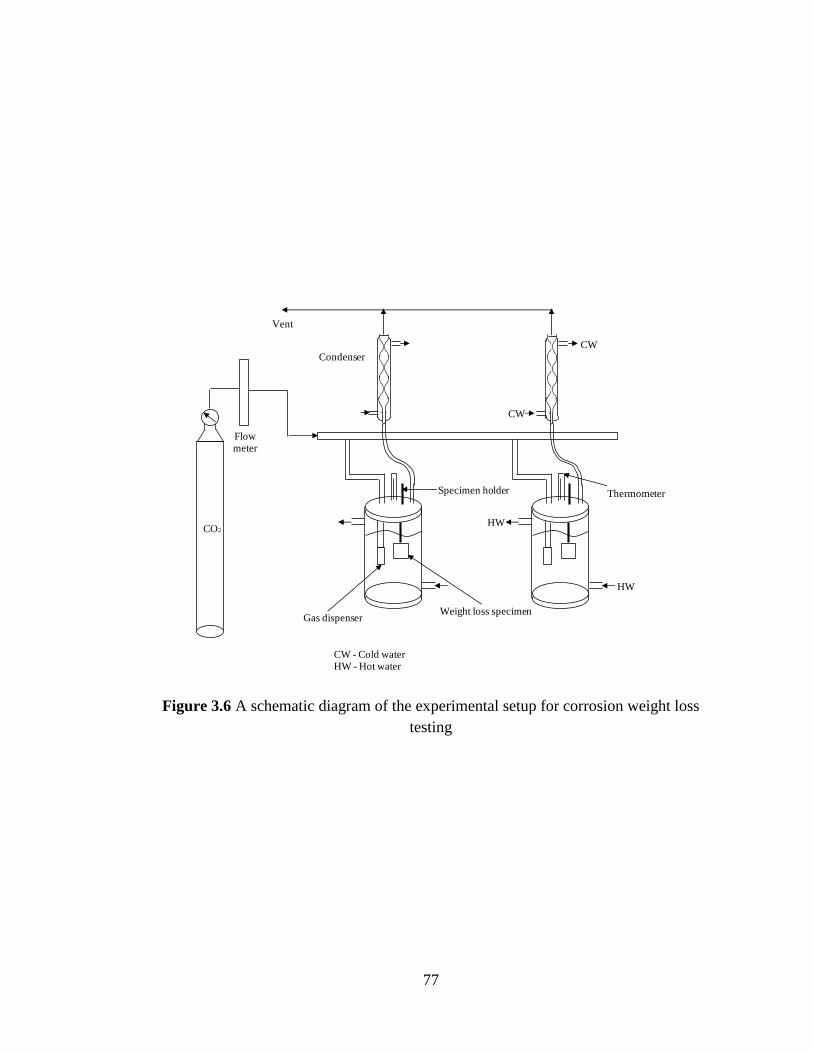
77

Figure 3.6 A schematic diagram of the experimental setup for corrosion weight loss

testing

Flowmeter

CO2

Vent

Condenser

Weight loss specimenGas dispenser

ThermometerSpecimen holder

HW

HW

CW

CW

CW - Cold water HW - Hot water

78

3.2.2.2 Specimen preparation

Carbon steel 1018 (CS1018) specimens were used for the reasons discussed in

section 3.2.1.2. The specimens were rectangular coupons with dimensions of 2.5 cm in

height, 2.5 cm in width, and 0.3 cm thickness, as shown in Figure 3.7. They were surface

finished with 600 grit silicon papers, rinsed with high purity methanol followed by

deionized water, and finally dried before being introduced into the test solution.

3.2.2.3 Solution preparation

The solution preparation for weight loss testing follows the same procedure as

detailed in section 3.2.1.3 except for the volume of test solution, which was two liters in

this case. The solution was preloaded with CO2 until the saturation point and corrosion

inhibitor with a specific concentration was added as required.

3.2.2.4 Experimental procedure

The test solution was transferred to the corrosion cell. The prepared specimens

were weighed using a microbalance with an accuracy of ±0.10 mg, and then mounted

onto the glass specimen hooks fitted to the center of the metal lid. The specimens were

immersed in the test solution, and the metal lid was fastened to the corrosion cell. The

gaseous CO2 was purged continuously throughout the experiment to maintain the CO2

saturation in the test solution. Hot water was circulated in the outer jacket of the

corrosion cell to elevate the temperature of the solution to the required condition. The

solution concentration, CO2 loading, and solution temperature were regularly monitored

throughout the experiments. Owing to its relatively long testing time, the test solution

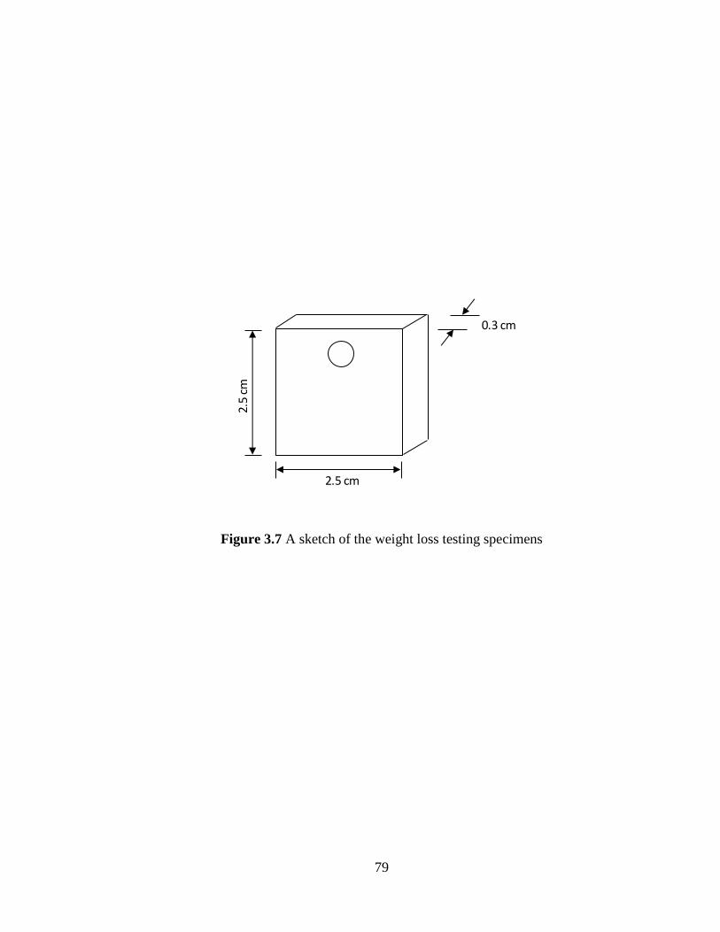
79

Figure 3.7 A sketch of the weight loss testing specimens

0.3 cm

2.5 cm

2.5

cm

80

required replenishment by addition of the calculated amounts of water at regular intervals

to account for the water loss by evaporation. The specimens were removed from the

corrosion cell at specific intervals of time. From the weight loss of these specimens,

corrosion rate was obtained.

3.2.2.5 Weight loss analysis

The corrosion products were removed from the tested specimens as per ASTM

standard G1-90 (1999). The tested specimens were cleaned mechanically by

simultaneous washing in running tap water and brushing with a non-metallic bristle to

remove the loose corrosion product and the weight loss compared to the initial weight of

the specimen was recorded. Then, the specimens were chemically cleaned by immersion

in a solution of concentrated hydrochloric acid (HCl) inhibited with 20 g antimony

trioxide (Sb2O3) and 50 g stannous chloride (SnCl2) for one minute. The mechanical and

chemical cleaning cycles were repeated, and the weight loss after each cycle was

determined. Determined weight loss was plotted against the number of cycles as shown

in Figure 3.8. The curve AB corresponds to the weight loss due to the removal of

corrosion product from the metal surface. As the corrosion product is removed, the bare

metal is exposed during the chemical cleaning and the measured weight loss in the

specimen became constant as shown in the curve BC. The point of intersection between

AB and BC corresponds to the weight loss due to corrosion from which the corrosion rate

can be calculated using Equation (3.3).

D

TA

WKCR

(3.3)

81

Figure 3.8 Estimation of weight loss of the tested specimen (ASTM G1-90)

0.36

0.37

0.37

0.38

0.38

0.39

0.39

0.40

0 2 4 6

Wei

gh

t lo

ss

Number of cleaning cycles

B

C

A

82

where CR is the corrosion rate in mmpy, K is the constant with a value of 8.76 x 104, W is

the weight loss in g, A is the area of the metal specimen in cm2, T is the time of exposure

in hours, and D is the density of the specimen in g/cm3.

3.2.2.6 Surface analysis

The weight loss specimen exposed to the longest duration of testing was subjected

to the surface analytical techniques including X-ray Diffraction analysis (XRD), Energy-

dispersive X-ray Spectroscopy (EDS), and Scanning Electron Microscopy (SEM) to

understand and characterize the corrosion products for different conditions tested. The

XRD analysis was carried out to characterize any crystalline phases in the corrosion

products. A Bruker Discover diffractometer (nickel - filtered Cu K - 0.154056 nm as a

radiation source) was used for analysis, and reference data from the International Centre

for Diffraction Data (ICDD) was used for identifying the phases. For the SEM analysis, a

JSM – 5600 (JEOL, USA) microscope was used for obtaining the images at different

magnifications. The EDS analysis was carried out using an EDAX Genesis 7000 model,

which was used for elemental analysis of the specimen surface. Following by surface

analysis, the specimens were subjected to a cleaning procedure as detailed in Section

3.2.2.5 to determine the weight loss and, in turn, the corrosion rate.

83

4. RESULTS AND DISCUSSION

The inhibition performance of the selected corrosion inhibitors was evaluated

using two corrosion testing techniques, namely electrochemical and weight loss testing.

The electrochemical testing provides an insight into the behaviour of corrosion and

corrosion inhibition while the weight loss testing provides information of corrosion

magnitudes in longer periods of exposure time than the electrochemical testing. Details of

results from both tests are given below.

4.1 Electrochemical tests

Corrosion characteristics of uninhibited and inhibited systems were studied by

evaluating the corrosion behaviour of carbon steel (CS1018) at different experimental

conditions as shown in Table 4.1. Electrochemical tests employed two techniques,

namely DC - cyclic potentiodynamic polarization and AC - impedance analysis.

4.1.1 Corrosion behaviour of uninhibited MEA systems

a) Absence of process contaminants

From the cyclic potentiodynamic polarization curve (Figure 4.1a), it can be

observed that the carbon steel exhibits active-passive behaviour in the uninhibited MEA

system (5.0 kmol/m3 MEA at 80

oC and 0.55 mol/mol CO2). Under these experimental

conditions, the metal undergoes active corrosion at a rate of 4.27 mmpy (Table 4.2).

Negative hysteresis (reverse curve lies left of the forward curve) suggests no pitting

corrosion tendency (Figure 4.1a).

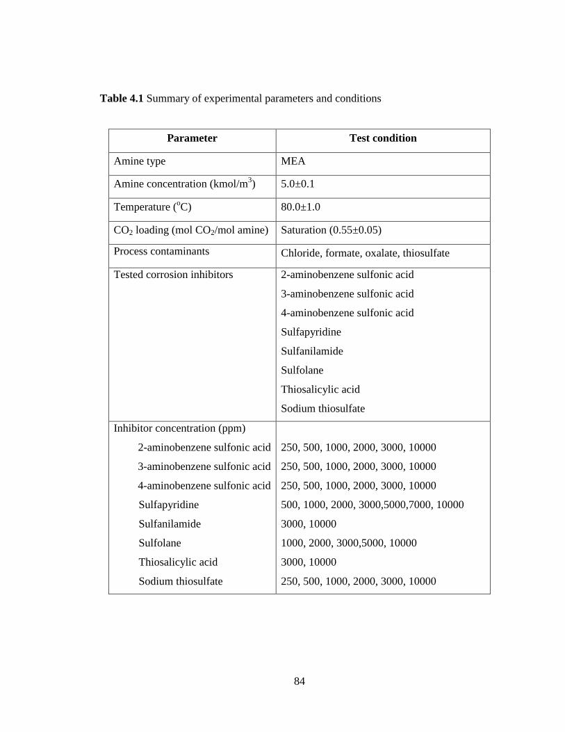
84

Table 4.1 Summary of experimental parameters and conditions

Parameter Test condition

Amine type MEA

Amine concentration (kmol/m3) 5.0±0.1

Temperature (oC) 80.0±1.0

CO2 loading (mol CO2/mol amine) Saturation (0.55±0.05)

Process contaminants Chloride, formate, oxalate, thiosulfate

Tested corrosion inhibitors 2-aminobenzene sulfonic acid



Sulfapyridine

Sulfanilamide

Sulfolane

Thiosalicylic acid

Sodium thiosulfate

Inhibitor concentration (ppm)




Sulfapyridine

Sulfanilamide

Sulfolane

Thiosalicylic acid

Sodium thiosulfate

250, 500, 1000, 2000, 3000, 10000

250, 500, 1000, 2000, 3000, 10000

250, 500, 1000, 2000, 3000, 10000

500, 1000, 2000, 3000,5000,7000, 10000

3000, 10000

1000, 2000, 3000,5000, 10000

3000, 10000

250, 500, 1000, 2000, 3000, 10000

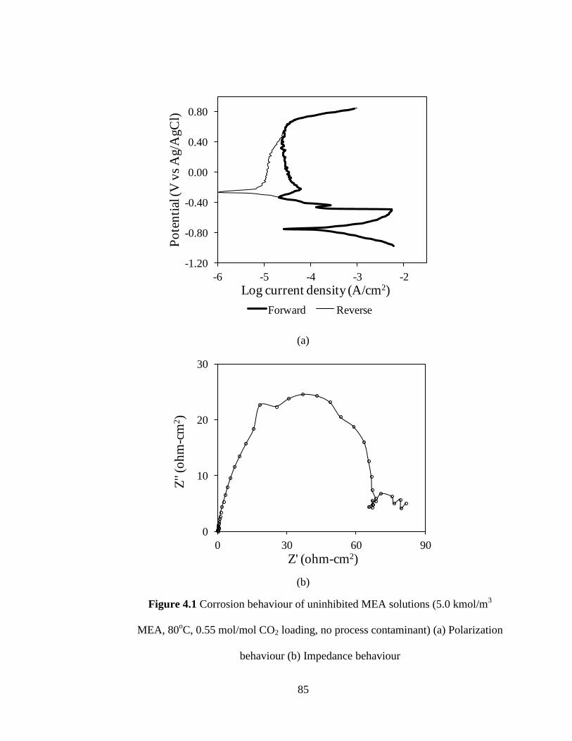
85

(a)

(b)

Figure 4.1 Corrosion behaviour of uninhibited MEA solutions (5.0 kmol/m3

MEA, 80oC, 0.55 mol/mol CO2 loading, no process contaminant) (a) Polarization

behaviour (b) Impedance behaviour

-1.20

-0.80

-0.40

0.00

0.40

0.80

-6 -5 -4 -3 -2

Po

ten

tial

(V

vs

Ag/A

gC

l)

Log current density (A/cm2)

Forward Reverse

0

10

20

30

0 30 60 90

Z''

(oh

m-c

m2)

Z' (ohm-cm2)

86

Table 4.2 Summary of electrochemical experimental results

Experimental Condition pH σ

(mS/cm)

Ecorr

(mV vs

Ag/AgCl)

icorr

(μA/cm2)

βc

(mV/

decade)

βa

(mV/

decade)

Rp

(ohm-cm2)

CR

(mmpy)

IE

(%)

Pitting

tendency

No corrosion inhibitor :

5.0 kmol/m3 MEA, 80oC,

α=0.55

- 8.15±0.03 42.55±1.75 -751.92±0.70 364.24±1.19 88.84±11.20 146.08±27.1 72.04±0.40 4.27±0.01 - No

10000 ppm

thiosulfate 8.78±0.05 39.44±1.20 -703.05±0.61 20.33±0.73 98.82±3.10 135.71±6.40 995.19±25.01 0.26±0.01 - No

10000 ppm

oxalate 8.24±0.02 43.24±2.60 -773.31±5.44 66.89±0.60 133.10±0.10 77.60±2.60 172.50±8.60 0.78±0.01 - No

10000 ppm

formate 7.98±0.03 50.67±1.60 -756.42±1.23 45.03±1.39 83.64±8.62 159.30±11.26 73.10±11.12 5.29±0.02 - No

10000 ppm

chloride 8.36±0.04 45.20±2.20 -750.34±0.74 344.37±2.15 71.60±3.40 120.90±6.30 86.84±2.40 4.04±0.03 - No

2-aminobenzene sulfonic

acid :


α=0.55, No process

contaminant

250 ppm 8.22±0.01 42.08±1.80 -787.91±0.71 47.02±0.83 123.73±2.20 63.58±1.30 390.21±6.90 0.55±0.01 87 No

500 ppm 8.30±0.04 41.40±1.40 -773.40±3.14 48.68±1.26 128.42±1.60 66.36±4.56 359.44±10.36 0.57±0.01 87 No

1000 ppm 8.37±0.02 40.06±2.10 -786.44±3.90 46.36±1.21 127.40±0.52 71.20±3.24 417.84±4.10 0.54±0.01 87 No

2000 ppm 8.48±0.02 38.87±1.20 -786.71±0.74 39.40±2.40 119.40±1.04 65.86±2.64 401.16±21.54 0.46±0.00 89 No

3000 ppm 8.60±0.01 37.95±0.80 -778.93±4.30 47.02±1.74 129.14±3.00 63.54±2.42 349.76±12.73 0.55±0.00 87 No

10000 ppm 8.80±0.06 36.60±2.40 -753.92±5.84 138.08±1.27 121.42±2.60 73.10±8.26 133.54±11.40 1.62±0.01 62 No


acid (1000 ppm) :


α=0.55

10000 ppm

formate 8.20±0.02 47.78±3.40 -742.36±8.24 52.65±0.50 90.74±8.46 127.73±2.12 84.70±3.26 5.70±0.01 -34 No

10000 ppm

chloride 8.47±0.02 46.95±2.90 -762.84±2.80 486.76±1.42 175.50±1.88 86.93±4.78 380.57±5.60 0.62±0.00 86 No


acid:


α=0.55, No process

contaminant

250 ppm 8.21±0.02 41.98±2.20 -740.56±7.20 41.39±1.16 116.50±1.70 55.23±2.03 391.74±8.90 0.49±0.01 89 No

500 ppm 8.27±0.01 41.63±1.60 -766.08±5.84 40.73±0.41 122.82±8.24 67.94±5.02 427.51±12.40 0.48±0.01 89 No

1000 ppm 8.35±0.03 40.72±3.10 -764.12±13.80 40.73±3.18 110.30±6.81 62.36±2.73 368.94±21.02 0.48±0.04 89±1 No

2000 ppm 8.47±0.02 40.10±1.80 -768.61±2.42 41.72±3.77 120.10±16.22 69.42±8.50 387.02±24.01 0.49±0.04 89±1 No

3000 ppm 8.63±0.01 39.31±1.50 -760.60±3.84 42.05±2.05 122.64±0.14 66.06±1.18 407.20±3.51 0.49±0.02 89±1 No

10000 ppm 8.71±0.01 37.91±2.30 -732.42±5.82 324.83±1.41 120.86±2.83 172.40±7.80 88.24±2.83 3.81±0.02 11±1 No


acid (1000 ppm) :


α=0.55

10000 ppm

formate 7.92±0.04 49.28±1.70 -747.81±6.23 453.64±1.85 199.40±3.12 141.12±0.80 105.42±13.30 5.31±0.02 -24±1 No

10000 ppm

chloride 8.45±0.03 44.02±2.10 -772.11±4.78 140.73±1.06 162.90±4.20 104.78±5.23 87.90±9.78 1.65±0.01 61 Yes

87

Table 4.2 Summary of electrochemical experimental results (continued)


(mS/cm)

Ecorr

(mV vs

Ag/AgCl)

icorr

(μA/cm2)

βc

(mV/

decade)

βa

(mV/

decade)

Rp

(ohm-cm2)

CR

(mmpy)

IE

(%)

Pitting

tendency


acid :


α=0.55, No process

contaminant

250 ppm 8.21±0.02 42.30±2.30 -766.61±0.30 47.68±2.95 132.74±3.90 71.60±3.34 400.94±7.40 0.56±0.04 87±1 No

500 ppm 8.26±0.01 41.69±2.60 -769.45±2.54 45.36±0.26 130.56±4.12 70.84±8.91 459.90±24.04 0.54±0.02 88 No

1000 ppm 8.35±0.02 41.44±1.80 -786.20±6.80 38.41±1.46 126.45±2.04 60.10±6.10 440.90±9.31 0.45±0.02 90 No

2000 ppm 8.42±0.01 40.86±2.10 -791.56±9.72 35.10±5.62 115.21±6.70 69.22±13.31 419.18±0.94 0.41±0.07 90±2 No

3000 ppm 8.54±0.01 39.90±1.60 -779.47±5.04 32.68±2.60 99.20±13.45 53.10±5.94 355.16±3.80 0.38±0.03 91±1 No

10000 ppm 8.70±0.03 37.82±3.20 -736.67±2.48 321.19±2.68 85.60±9.05 108.70±12.32 99.14±4.20 3.77±0.03 12±1 No


acid (1000 ppm) :


α=0.55

10000 ppm

formate 8.24±0.02 50.02±4.10 -748.30±3.42 463.58±2.09 122.22±8.65 149.91±8.30 86.63±6.70 5.45±0.02 -28 No

10000 ppm

chloride 8.45±0.03 46.04±1.20 -776.51±1.50 39.74±0.83 121.8±10.0 62.44±3.10 385.24±8.90 0.46±0.03 89 No

Sulfapyridine :


α=0.55, No process

contaminant

500 ppm 8.25±0.03 42.45±1.80 -748.72±2.12 364.24±0.79 99.50±2.62 142.94±1.23 86.30±5.92 4.26±0.01 0 No

1000 ppm 8.29±0.01 42.38±1.40 -746.44±8.64 261.26±2.75 151.16±1.83 106.41±3.24 104.54±12.10 3.07±0.03 28±1 No

2000 ppm 8.42±0.01 41.02±3.10 -783.82±6.89 37.42±2.19 126.92±4.90 69.30±5.78 468.68±9.72 0.44±0.03 90±1 No

3000 ppm 8.58±0.02 39.39±2.60 -796.17±5.43 35.43±1.69 118.60±5.92 63.30±11.12 396.78±6.14 0.42±0.02 90±1 No

5000 ppm 8.63±0.03 38.27±1.70 -783.27±4.82 326.49±1.08 122.53±9.18 65.74±13.23 444.70±4.28 0.38±0.01 91 No

7000 ppm 8.71±0.04 37.65±3.30 -784.67±3.69 34.77±3.16 122.65±4.70 59.91±6.41 407.66±3.20 0.41±0.03 90±1 No

10000 ppm 8.76±0.04 36.41±4.10 -786.21±9.12 28.21±4.01 121.50±9.92 64.26±8.14 527.91±1.20 0.33±0.05 92±1 No

Sulfapyridine (2000 ppm) :


α=0.55

10000 ppm

formate 8.25±0.01 47.32±2.60 -778.44±7.43 44.37±2.68 135.36±4.12 58.66±10.12 358.50±9.45 0.52±0.03 88±1 No

10000 ppm

chloride 8.45±0.03 48.59±1.10 -741.95±12.12 37.09±2.53 107.40±3.87 165.56±7.96 90.92±4.20 4.34±0.03 -2±1 No

Sulfanilamide:


α=0.55, No process

contaminant

3000 ppm 8.16±0.01 42.12±1.80 -767.61±8.20 212.91±1.52 148.64±8.70 97.34±6.40 103.60±6.80 2.50±0.02 42±1 No

10000 ppm 8.25±0.03 41.69±2.40 -744.82±4.60 291.06±2.07 76.42±10.40 131.32±8.12 84.30±4.80 3.41±0.02 20±1 No

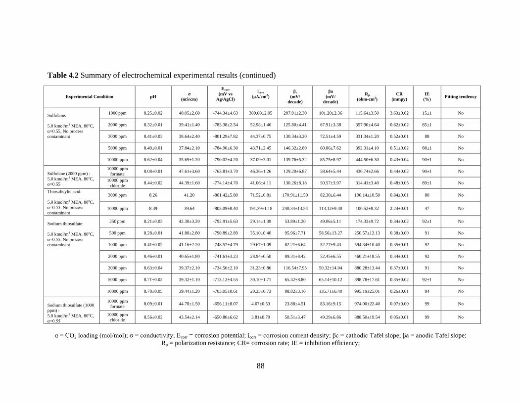
88

Table 4.2 Summary of electrochemical experimental results (continued)

α = CO2 loading (mol/mol); σ = conductivity; Ecorr = corrosion potential; icorr = corrosion current density; βc = cathodic Tafel slope; βa = anodic Tafel slope;

Rp = polarization resistance; CR= corrosion rate; IE = inhibition efficiency;


(mS/cm)

Ecorr

(mV vs

Ag/AgCl)

icorr

(μA/cm2)

βc

(mV/

decade)

βa

(mV/

decade)

Rp

(ohm-cm2)

CR

(mmpy)

IE

(%) Pitting tendency

Sulfolane:


α=0.55, No process

contaminant

1000 ppm 8.25±0.02 40.05±2.60 -744.34±4.63 309.60±2.05 207.91±2.30 101.20±2.36 115.64±3.50 3.63±0.02 15±1 No

2000 ppm 8.32±0.01 39.41±1.40 -783.38±2.54 52.98±1.46 125.80±4.41 67.91±3.38 357.90±4.64 0.62±0.02 85±1 No

3000 ppm 8.41±0.03 38.64±2.40 -801.29±7.82 44.37±0.75 130.34±3.20 72.51±4.59 331.34±1.20 0.52±0.01 88 No

5000 ppm 8.49±0.01 37.84±2.10 -784.90±6.30 43.71±2.45 146.32±2.80 60.86±7.62 392.31±4.10 0.51±0.02 88±1 No

10000 ppm 8.62±0.04 35.69±1.20 -790.02±4.20 37.09±3.01 139.76±5.32 85.75±8.97 444.50±6.30 0.43±0.04 90±1 No

Sulfolane (2000 ppm) :


α=0.55

10000 ppm

formate 8.08±0.01 47.61±3.60 -763.81±3.70 46.36±1.26 129.20±6.87 58.64±5.44 430.74±2.66 0.44±0.02 90±1 No

10000 ppm

chloride 8.44±0.02 44.39±1.60 -774.14±4.70 41.06±4.11 130.26±8.18 50.57±3.97 314.41±3.40 0.48±0.05 89±1 No

Thiosalicylic acid:


α=0.55, No process

contaminant

3000 ppm 8.26 41.20 -801.42±5.80 71.52±0.81 170.91±11.50 82.30±6.44 190.14±10.50 0.84±0.01 80 No

10000 ppm 8.39 39.64 -803.09±8.40 191.39±1.18 240.34±13.54 113.12±9.40 100.52±8.32 2.24±0.01 47 No

Sodium thiosulfate:


α=0.55, No process

contaminant

250 ppm 8.21±0.03 42.30±3.20 -792.91±5.63 29.14±1.39 53.80±1.20 49.06±5.11 174.33±9.72 0.34±0.02 92±1 No

500 ppm 8.28±0.01 41.80±2.80 -790.89±2.89 35.10±0.40 95.96±7.71 58.56±13.27 250.57±12.13 0.38±0.00 91 No

1000 ppm 8.41±0.02 41.16±2.20 -748.57±4.79 29.67±1.09 82.21±6.64 52.27±9.43 594.34±10.40 0.35±0.01 92 No

2000 ppm 8.46±0.01 40.65±1.80 -741.61±3.23 28.94±0.50 89.31±8.42 52.45±6.55 460.21±18.55 0.34±0.01 92 No

3000 ppm 8.63±0.04 39.37±2.10 -734.50±2.10 31.23±0.86 116.54±7.95 50.32±14.04 880.28±13.44 0.37±0.01 91 No

5000 ppm 8.71±0.02 39.32±1.10 -713.12±4.55 30.10±1.71 65.42±8.80 65.14±10.12 898.78±17.61 0.35±0.02 92±1 No

10000 ppm 8.78±0.05 39.44±1.20 -703.05±0.61 20.33±0.73 98.82±3.10 135.71±6.40 995.19±25.01 0.26±0.01 94 No

Sodium thiosulfate (1000

ppm) :


α=0.55

10000 ppm

formate 8.09±0.01 44.78±1.50 -656.11±8.07 4.67±0.53 23.88±4.51 83.16±9.15 974.00±22.40 0.07±0.00 99 No

10000 ppm

chloride 8.56±0.02 43.54±2.14 -650.80±6.62 3.81±0.79 50.51±3.47 49.29±6.86 888.50±19.54 0.05±0.01 99 No

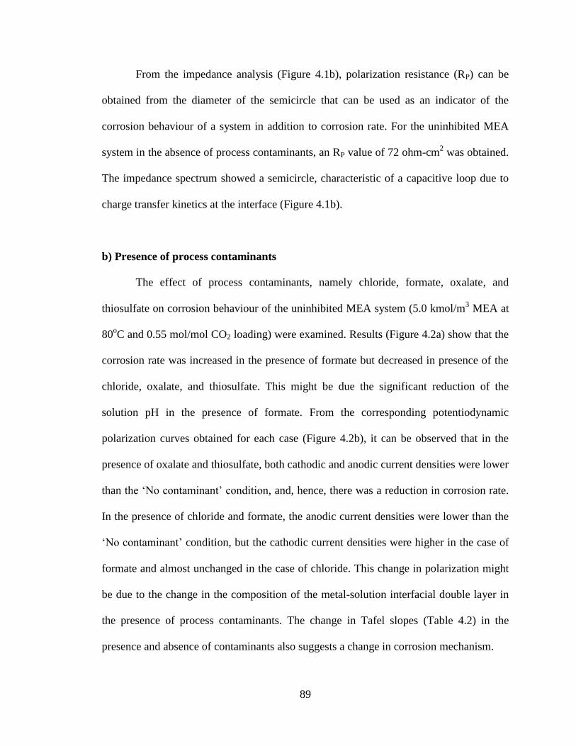
89

From the impedance analysis (Figure 4.1b), polarization resistance (RP) can be

obtained from the diameter of the semicircle that can be used as an indicator of the

corrosion behaviour of a system in addition to corrosion rate. For the uninhibited MEA

system in the absence of process contaminants, an RP value of 72 ohm-cm2 was obtained.

The impedance spectrum showed a semicircle, characteristic of a capacitive loop due to

charge transfer kinetics at the interface (Figure 4.1b).

b) Presence of process contaminants

The effect of process contaminants, namely chloride, formate, oxalate, and

thiosulfate on corrosion behaviour of the uninhibited MEA system (5.0 kmol/m3 MEA at

80oC and 0.55 mol/mol CO2 loading) were examined. Results (Figure 4.2a) show that the

corrosion rate was increased in the presence of formate but decreased in presence of the

chloride, oxalate, and thiosulfate. This might be due the significant reduction of the

solution pH in the presence of formate. From the corresponding potentiodynamic

polarization curves obtained for each case (Figure 4.2b), it can be observed that in the

presence of oxalate and thiosulfate, both cathodic and anodic current densities were lower

than the ‘No contaminant’ condition, and, hence, there was a reduction in corrosion rate.

In the presence of chloride and formate, the anodic current densities were lower than the

‘No contaminant’ condition, but the cathodic current densities were higher in the case of

formate and almost unchanged in the case of chloride. This change in polarization might

be due to the change in the composition of the metal-solution interfacial double layer in

the presence of process contaminants. The change in Tafel slopes (Table 4.2) in the

presence and absence of contaminants also suggests a change in corrosion mechanism.

90

(a) (b)

(c) (d)

Figure 4.2 Corrosion behaviour of uninhibited MEA solutions with and without process

contaminants (5.0 kmol/m3 MEA, 80

oC, 0.55 mol/mol CO2 loading) (a) Comparison of

corrosion rate (b) Polarization behaviour (c) Comparison of polarization resistance

(d) Impedance behaviour

0.00

1.00

2.00

3.00

4.00

5.00

6.00

No

proc

ess

cont

amin

ant

chlo

ride

form

ate

oxal

ate

thio

sulf

ate

Co

rosi

on r

ate

(m

mp

y)

-1.10

-1.00

-0.90

-0.80

-0.70

-0.60

-0.50

-0.40

-6 -5 -4 -3 -2 -1

Po

ten

tial

(V

vs

Ag/A

gC

l)

Log current density (A/cm2)No process contaminant chlorideformate oxalatethiosulfate

0

200

400

600

800

1000

1200

No

proc

ess

cont

amin

ant

chlo

ride

form

ate

oxal

ate

thio

sulf

ate

RP

(oh

m c

m2)

0

200

400

600

800

0 200 400 600

Z''

(oh

m-c

m2)

Z' (ohm-cm2)No process contaminant chlorideformate oxalatethiosulfate

91

Pitting tendency was not induced by the presence of process contaminants.

Polarization resistance (RP) values obtained from impedance analysis in the

absence and presence of different process contaminants can also be used to explain the

change in corrosion behaviour of the system. From Figure 4.2c, it can be observed that

the RP values in the presence of chloride and formate were comparable to the ‘No

contaminant’ result. In the case of oxalate and thiosulfate, RP values were higher,

representing a reduced corrosivity of the system (Figure 4.2c). The impedance behaviour

of thiosulfate was different from the other process contaminants. An impedance spectrum

corresponding to the ‘No contaminant’ condition and the presence of chloride, formate,

and oxalate showed a semicircle, characteristic of a capacitive loop due to charge transfer

kinetics at the interface (Figure 4.2d). In the case of thiosulfate, in addition to the

semicircle, the low frequency end (right end of X axis) of the spectrum was characterized

by linearity (diffusion tail). This might be due to the thin black film formed over the

metal surface by the adsorption of thiosulfate molecules (S2O32-

) limiting the diffusion of

corrosive species across the interface.

Based on the above results, formate, which increased the corrosion rate of the

uninhibited MEA system, was chosen to be tested for the effect on corrosion inhibition

performance of selected inhibitors. Though chloride does not increase the corrosion rate,

it can potentially cause localized pitting corrosion, and, hence, it is important to study the

effect of chloride on the performance of inhibitors. Consequently, in order to evaluate the

performance of the inhibitors, only the effect of formate and chloride were studied.

Oxalate was not tested due to its reduction of corrosion rate in uninhibited MEA systems,

and thiosulfate was tested for its inhibition performance.

92

4.1.2 Corrosion behaviour of inhibited MEA systems

The selected corrosion inhibitors (Table 4.1) were tested at different

concentrations. Changes in the corrosion behaviour of carbon steel in different inhibited

MEA systems (5.0 kmol/m3 MEA at 80

oC and 0.55 mol/mol CO2 loading) compared to

the uninhibited MEA systems were studied. The effect of process contaminants (chloride

and formate) on the performance of different corrosion inhibitors was also studied.

4.1.2.1 2-aminobenzene sulfonic acid


Corrosion inhibition performance of 2-aminobenzene sulfonic acid was tested as a

function of corrosion inhibitor concentration. From Figure 4.3a, it can be observed that

the corrosion rate of carbon steel in the 2-aminobenzene sulfonic acid inhibited MEA

system was significantly reduced (0.46 – 0.57 mmpy) compared to the uninhibited

corrosion rate of 4.27 mmpy, when the inhibitor concentration was in the range of 250 to

3000 ppm. However at 10,000 ppm, corrosion rate increased to 1.62 mmpy. Corrosion

inhibition efficiency was in the range of 87–89 % for the inhibitor concentration of 250 –

3000 ppm, which dropped to 62 % at 10,000 ppm (Figure 4.3b).

From the potentiodynamic polarization curves for the inhibited MEA systems

(Figure 4.3c), it can be observed that even though the metal undergoes active corrosion,

the cathodic current densities were lower than the uninhibited condition while the anodic

current densities were almost unchanged. This suggests that the corrosion inhibition was

cathodic in nature and was due to the preferential adsorption of inhibitor molecules onto

the cathodic sites of the metal surface.

93

(a) (b)

(c) (d)

(e)

Figure 4.3 Corrosion behaviour of ‘2-aminobenzene sulfonic acid’ inhibited MEA


oC, 0.55 mol/mol CO2 loading, no process contaminant)

(a) Comparison of corrosion rate (b) Comparison of inhibition efficiencies (c) Polarization

behaviour (d) Comparison of polarization resistance (e) Impedance behaviour

0.00

1.50

3.00

4.50

0 250 500 1000 2000 3000 10000

Co

rosi

on r

ate

(m

mp

y)



0%

25%

50%

75%

100%

250 500 1000 2000 3000 10000

Inh

ibit

ion

eff

icie

ncy

(%

)


-1.10

-0.90

-0.70

-0.50

-6 -5 -4 -3 -2

Po

ten

tial

(V

vs

Ag/A

gC

l)

Log current density (A/cm2)Uninhibited 250 ppm 500 ppm1000 ppm 2000 ppm 3000 ppm10000 ppm

0

100

200

300

400

500

0 250 500 1000 2000 3000 10000

RP

(oh

m-c

m2)



0

30

60

90

120

150

180

0 100 200 300 400 500

Z''

(oh

m-c

m2)

Z' (ohm-cm2)Uninhibited 250 ppm 500 ppm1000 ppm 2000 ppm 3000 ppm10000 ppm

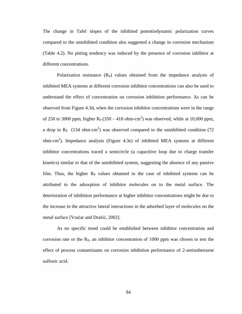
94

The change in Tafel slopes of the inhibited potentiodynamic polarization curves

compared to the uninhibited condition also suggested a change in corrosion mechanism

(Table 4.2). No pitting tendency was induced by the presence of corrosion inhibitor at

different concentrations.

Polarization resistance (RP) values obtained from the impedance analysis of

inhibited MEA systems at different corrosion inhibitor concentrations can also be used to

understand the effect of concentration on corrosion inhibition performance. As can be

observed from Figure 4.3d, when the corrosion inhibitor concentrations were in the range

of 250 to 3000 ppm, higher RP (350 – 418 ohm-cm2) was observed, while at 10,000 ppm,

a drop in RP (134 ohm-cm2) was observed compared to the uninhibited condition (72

ohm-cm2). Impedance analysis (Figure 4.3e) of inhibited MEA systems at different

inhibitor concentrations traced a semicircle (a capacitive loop due to charge transfer

kinetics) similar to that of the uninhibited system, suggesting the absence of any passive

film. Thus, the higher RP values obtained in the case of inhibited systems can be

attributed to the adsorption of inhibitor molecules on to the metal surface. The

deterioration of inhibition performance at higher inhibitor concentrations might be due to

the increase in the attractive lateral interactions in the adsorbed layer of molecules on the

metal surface [Vračar and Dražić, 2002].

As no specific trend could be established between inhibitor concentration and

corrosion rate or the RP, an inhibitor concentration of 1000 ppm was chosen to test the

effect of process contaminants on corrosion inhibition performance of 2-aminobenzene

sulfonic acid.

95


Inhibition performance of 2-aminobenzene sulfonic acid (1000 ppm) was almost

unaffected by the presence of chloride but was detrimentally affected by the presence of

formate. It can be observed that the corrosion rate in the presence of chloride (4.04

mmpy) was virtually unchanged compared to the ‘No contaminant’ results (Figure 4.4a).

However, in the presence of formate (5.29 mmpy), the corrosion rate was higher than the

uninhibited corrosion rates both with and without formate. It is more apparent from

Figure 4.4b, where the presence of formate was characterized by an aggravation (-33 %)

of corrosion. From the potentiodynamic polarization behaviour (Figure 4.4c), it can be

observed that in the case of chloride, both cathodic and anodic current densities were

slightly lower than the ‘No contaminant’ condition, but in case of formate, though the

anodic current densities were comparable, the cathodic current densities were much

higher than the ‘No contaminant’ condition. This suggests that the adsorption of inhibitor

molecules on the metal surface was disrupted and possibly displaced by the formate ions

from the contaminant. No pitting tendency was induced by the presence of the process

contaminants.

RP values obtained from the impedance analysis of the 2-aminobenzene sulfonic

acid (1000 ppm) inhibited MEA systems were also used to understand the effect of

process contaminants on the corrosion behaviour of the system. From Figure 4.4d, it can

be observed that in the presence of chloride, the RP was slightly lower, but in the

presence of formate, the RP was almost as low as the uninhibited system. From the

impedance analysis, it can be observed that a semicircular loop characteristic of charge

transfer kinetics was obtained, suggesting the absence of any passive film (Figure 4.4e).

96

(a) (b)

(c) (d)

(e)

Figure 4.4 Corrosion behaviour of inhibited MEA solutions with and without process


oC, 0.55 mol/mol CO2 loading, 1000 ppm 2-

aminobenzene sulfonic acid) (a) Comparison of corrosion rate (b) Comparison of

inhibition efficiencies (c) Polarization behaviour (d) Comparison of polarization


0.00

2.00

4.00

6.00

No process contaminant

chloride formate

Co

rosi

on r

ate

(m

mp

y)

Uninhibited Inhibited

-50%

-25%

0%

25%

50%

75%

100%


chloride formate

Inh

ibit

ion

eff

icie

ncy

(%

)


-1.10

-0.90

-0.70

-0.50

-7 -6 -5 -4 -3 -2

Po

ten

tial

(V

vs

Ag/A

gC

l)


No process contaminant chloride formate

0

150

300

450


chloride formate

RP

(oh

m-c

m2)


0

30

60

90

120

150

180

0 100 200 300 400

Z''

(oh

m-c

m2)

Z' (ohm-cm2)


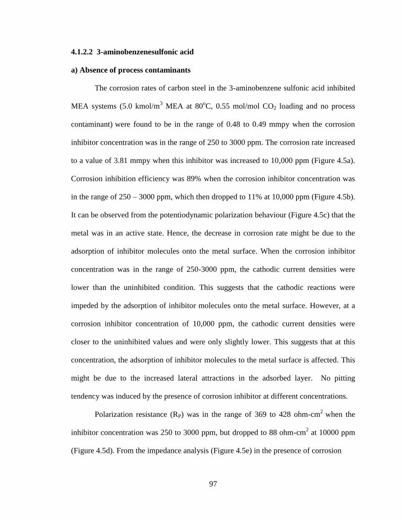
97

4.1.2.2 3-aminobenzenesulfonic acid


The corrosion rates of carbon steel in the 3-aminobenzene sulfonic acid inhibited

MEA systems (5.0 kmol/m3 MEA at 80

oC, 0.55 mol/mol CO2 loading and no process

contaminant) were found to be in the range of 0.48 to 0.49 mmpy when the corrosion

inhibitor concentration was in the range of 250 to 3000 ppm. The corrosion rate increased

to a value of 3.81 mmpy when this inhibitor was increased to 10,000 ppm (Figure 4.5a).

Corrosion inhibition efficiency was 89% when the corrosion inhibitor concentration was

in the range of 250 – 3000 ppm, which then dropped to 11% at 10,000 ppm (Figure 4.5b).

It can be observed from the potentiodynamic polarization behaviour (Figure 4.5c) that the

metal was in an active state. Hence, the decrease in corrosion rate might be due to the

adsorption of inhibitor molecules onto the metal surface. When the corrosion inhibitor

concentration was in the range of 250-3000 ppm, the cathodic current densities were

lower than the uninhibited condition. This suggests that the cathodic reactions were

impeded by the adsorption of inhibitor molecules onto the metal surface. However, at a

corrosion inhibitor concentration of 10,000 ppm, the cathodic current densities were

closer to the uninhibited values and were only slightly lower. This suggests that at this

concentration, the adsorption of inhibitor molecules to the metal surface is affected. This

might be due to the increased lateral attractions in the adsorbed layer. No pitting

tendency was induced by the presence of corrosion inhibitor at different concentrations.

Polarization resistance (RP) was in the range of 369 to 428 ohm-cm2

when the

inhibitor concentration was 250 to 3000 ppm, but dropped to 88 ohm-cm2 at 10000 ppm

(Figure 4.5d). From the impedance analysis (Figure 4.5e) in the presence of corrosion

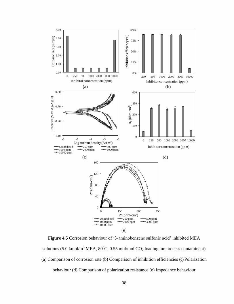
98

(a) (b)

(c) (d)

(e)






0.00

1.00

2.00

3.00

4.00

5.00

0 250 500 1000 2000 3000 10000

Co

rosi

on r

ate

(m

mp

y)


0%

25%

50%

75%

100%

250 500 1000 2000 3000 10000

Inh

ibit

ion

eff

icie

ncy

(%

)



-1.10

-0.90

-0.70

-0.50

-6 -5 -4 -3 -2

Po

ten

tial

(V

vs

Ag/A

gC

l)


0

150

300

450

600

0 250 500 1000 2000 3000 10000

RP

(oh

m-c

m2)


0

40

80

120

160

0 150 300 450

Z''

(oh

m-c

m2)


99

inhibitor, semicircular loops with larger diameters than the uninhibited condition could be

observed. Absence of a diffusion tail suggests that no passive film was formed. Thus, the

increase in RP might be due to the adsorption of inhibitor molecules onto the metal

surface. As no trend could be observed between the corrosion inhibitor concentration and

corrosion rate or RP, 1000 ppm was chosen to test the effects of process contaminants.


The presence of process contaminants (chloride or formate) had a deteriorating

effect on corrosion inhibition performance of 3-aminobenzene sulfonic acid (1000 ppm).

The corrosion rate in the presence of chloride increased to 1.65 mmpy from 0.48 mmpy

in the absence of any contaminant. In the case of formate, the corrosion rate was 5.31

mmpy, which was higher than the uninhibited corrosion rate both in the presence and

absence of formate (Figure 4.6a). The corrosion inhibition efficiency of 3-aminobenzene

sulfonic acid in the presence of chloride dropped to 62% compared to the ‘No

contaminant’ condition (89%). In the presence of formate, an efficiency of -24% was

observed, suggesting that the inhibitor actually aggravated the corrosion (Figure 4.6b).

From the potentiodynamic polarization analysis (Figure 4.6c), it can be observed that the

metal underwent active corrosion, and the cathodic current densities were characterized

by higher values in the presence of contaminant than the ‘No contaminant’ condition.

This might be due to the disruption of adsorption of corrosion inhibitor molecules onto

the metal surface in the presence of process contaminants, and this effect is more

pronounced in the presence of formate than chloride. From the cyclic polarization

analysis (Figure 4.7a), positive hysteresis (reverse curve lies to the right of the forward

100

(a) (b)

(c) (d)

(e)







0.00

2.00

4.00

6.00


chloride formate

Co

rosi

on r

ate

(m

mp

y)


-50%

-25%

0%

25%

50%

75%

100%


chloride formate

Inh

ibit

ion

eff

icie

ncy

(%

)


-1.10

-0.90

-0.70

-0.50

-7 -6 -5 -4 -3 -2

Po

ten

tial

(V

vs

Ag/A

gC

l)



0

200

400


chloride formate

RP

(oh

m-c

m2)


0

30

60

90

120

150

180

0 100 200 300 400

Z''

(oh

m-c

m2)

Z' (ohm-cm2)

No process contaminant formate chloride

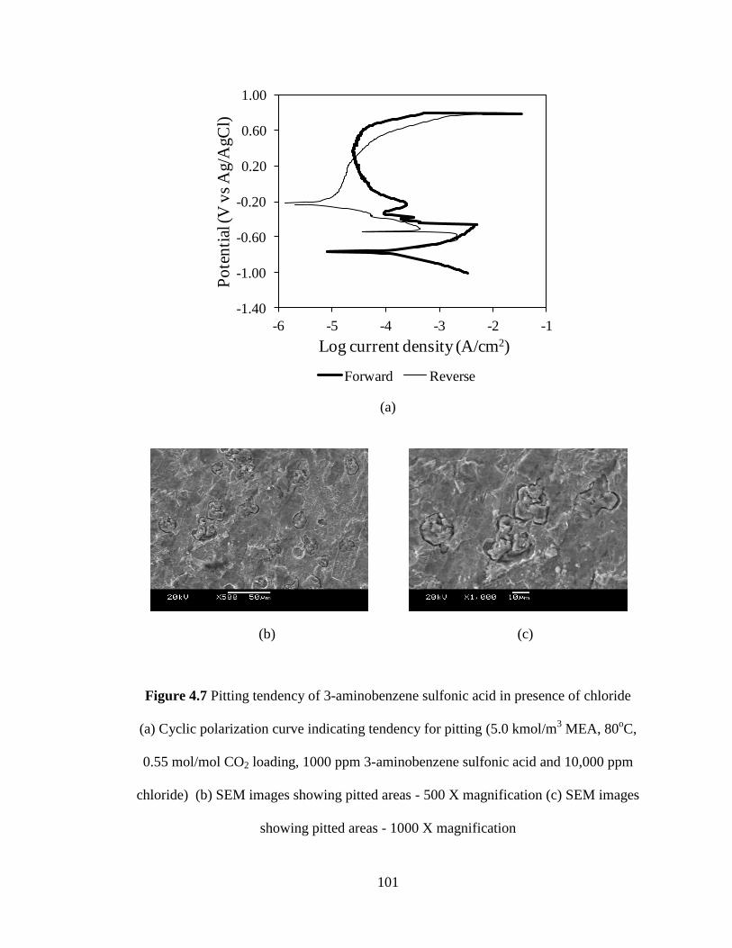
101

(a)

(b) (c)

Figure 4.7 Pitting tendency of 3-aminobenzene sulfonic acid in presence of chloride

(a) Cyclic polarization curve indicating tendency for pitting (5.0 kmol/m3 MEA, 80

oC,

0.55 mol/mol CO2 loading, 1000 ppm 3-aminobenzene sulfonic acid and 10,000 ppm

chloride) (b) SEM images showing pitted areas - 500 X magnification (c) SEM images

showing pitted areas - 1000 X magnification

-1.40

-1.00

-0.60

-0.20

0.20

0.60

1.00

-6 -5 -4 -3 -2 -1

Po

ten

tial

(V

vs

Ag/A

gC

l)


Forward Reverse

102

curve) was observed in the presence of chloride, suggesting the possibility of pitting

corrosion. SEM analysis of the working electrode after the experiment confirmed the

occurrence of pitting corrosion (Figure 4.7b and Figure 4.7c).

Polarization resistances (RP) obtained from the impedance analysis corroborated

the observation from the potentiodynamic polarization analyses. The deterioration of

corrosion inhibition performance in the presence of process contaminants was

characterized by a drop in RP to the value of 88 ohm-cm2 in the presence of chloride and

105 ohm-cm2 in the case of formate from 369 ohm-cm

2 for the ‘No contaminant’

condition (Figure 4.6d). From the impedance analysis (Figure 4.6e), the semicircular loop

obtained was characteristic of a dissolution process taking place at the metal/solution

interface. The lower RP values in the presence of process contaminants might be

attributed to the interference in the adsorption of corrosion inhibitor onto the metal

surface by the chloride or formate ions.

4.1.2.3 4-aminobenzenesulfonic acid


Corrosion rates of carbon steel in 4-aminobenzene sulfonic acid inhibited MEA

systems (5.0 kmol/m3 MEA at 80

oC, 0.55 mol/mol CO2 loading and no process

contaminant) were in the range of 0.38 to 0.56 mmpy when the corrosion inhibitor

concentrations were 250 to 3000 ppm but increased to 3.77 mmpy at 10,000 ppm (Figure

4.8a). Corrosion inhibition efficiencies were in the range of 87 to 91% when the inhibitor

concentration was 250 to 3000 ppm, which dropped to 12% at 10,000 ppm (Figure 4.8b).

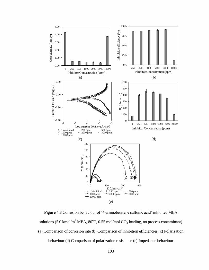
103

(a) (b)

(c) (d)

(e)






0.00

1.00

2.00

3.00

4.00

5.00

0 250 500 1000 2000 3000 10000

Co

rosi

on r

ate

(m

mp

y)

Inhibitor Concentration (ppm)


0%

25%

50%

75%

100%

250 500 1000 2000 3000 10000

Inh

ibit

ion

eff

icie

ncy

(%

)



-1.10

-0.90

-0.70

-0.50

-6 -5 -4 -3 -2

Po

ten

tial

(V

vs

Ag/A

gC

l)


0

100

200

300

400

500

600

0 250 500 1000 2000 3000 10000

Rp(o

hm

-cm

2)



0

30

60

90

120

150

180

0 150 300 450

Z''

(oh

m-c

m2)


104

From the potentiodynamic polarization curves (Figure 4.8c), it can be observed that even

though the metal undergoes active corrosion, lower corrosion rates were obtained in the

presence of corrosion inhibitor. This can be attributed to the adsorption of inhibitor

molecules onto the metal surface. At the corrosion inhibitor concentrations of 250 - 3000

ppm, the cathodic current densities were lower than the uninhibited cathodic current

densities suggesting that the cathodic reactions were highly impeded by the adsorption of

corrosion inhibitor. No pitting tendency was induced by the presence of corrosion

inhibitor at any concentration.

Polarization resistances (RP) obtained from the impedance analysis at different

concentrations of corrosion inhibitor corroborated the inferences from the

potentiodynamic polarization analysis. At the inhibitor concentration of 250 - 3000 ppm,

RP values obtained were in the range of 355 - 460 ohm-cm2, which dropped to 99 ohm-

cm2 at 10,000 ppm (Figure 4.8d). The deterioration of performance at higher inhibitor

concentrations might be due to the increase in the attractive lateral interactions in the

adsorbed layer of molecules on the metal surface [Vračar and Dražić, 2002]. Impedance

analysis yielded a semicircle characteristic of charge transfer kinetics at the metal-

solution interface, suggesting that no passive layer might be present (Figure 4.8e).

Hence, the increase in RP value might be due to the adsorption of inhibitor molecules

onto the metal surface. As no specific trend between corrosion inhibitor concentration

and corrosion rate or RP could be observed, a corrosion inhibitor concentration of 1000

ppm was chosen to test the effect of process contaminants on inhibition performance of

4-aminobenzene sulfonic acid.

105


Corrosion inhibition performance of 4-aminobenzene sulfonic acid (1000 ppm)

was almost unaffected by the presence of chloride but deteriorated in the presence of

formate. While the corrosion rate in the presence of chloride was 0.46 mmpy, the

corrosion rate in the presence of formate was 5.45 mmpy compared to the corrosion rate

in the absence of any contaminant, which was 0.45 mmpy (Figure 4.9a). Corrosion

inhibition efficiency in the presence of chloride was 89% and in the presence of formate

was -28%, implying that the corrosion rate of the system was increased by the inhibitor in

the presence of formate (Figure 4.9b). From the potentiodynamic polarization behaviour

(Figure 4.9c), it can be observed that the metal underwent active corrosion, and in the

presence of chloride, the anodic and cathodic current densities were virtually the same as

those of the ‘No contaminant’ condition, but in the presence of formate, the cathodic

current densities were much higher in comparison. An increase in corrosion rate in the

presence of formate might be caused by the interference of formate ions in the adsorption

of inhibitor molecules onto the metal surface. No pitting tendency was present in either

case.

While the polarization resistance (RP) in the presence of chloride was slightly

lower (385 ohm-cm2) than the no contaminant condition (441 ohm-cm

2), RP in the

presence of formate was drastically lower (87 ohm-cm2) (Figure 4.9d). From the

impedance analysis (Figure 4.9e), it can be observed that a semicircular loop

characteristic of charge transfer kinetics was obtained. The lower values of RP in the

presence of formate might be due to the interference of formate ions in the adsorption of

inhibitor molecules onto the metal surface.

106

(a) (b)

(c) (d)

(e)







0.00

2.00

4.00

6.00


chloride formate

Co

rosi

on r

ate

(m

mp

y)


-50%

-25%

0%

25%

50%

75%

100%


chloride formate

Inh

ibit

ion

eff

icie

ncy

(%

)


-1.10

-0.90

-0.70

-0.50

-7 -6 -5 -4 -3 -2

Po

ten

tial

(V

vs

Ag/A

gC

l)



0

100

200

300

400

500


chloride formate

RP

(oh

m-c

m2)


0

30

60

90

120

150

180

0 150 300 450

Z''

(oh

m-c

m2)

Z' (ohm-cm2)


107

4.1.2.4 Sulfapyridine


Corrosion rates of carbon steel in sulfapyridine inhibited MEA systems (5.0

kmol/m3 MEA at 80

oC, 0.55 mol/mol CO2 loading and no process contaminant) were in

the range of 0.33-0.44 mmpy when the inhibitor concentrations were in the range of

2000-10,000 ppm. While the corrosion rate was slightly lower at an inhibitor

concentration of 1000 ppm (3.07 mmpy), at 500 ppm (4.26 mmpy), the corrosion rate

was almost as high as the uninhibited corrosion rate (4.27 mmpy) (Figure 4.10a).

Corrosion inhibition efficiencies were in the range of 90–91% when the inhibitor

concentrations were in the range of 2000-10,000 ppm (Figure 4.10b). At inhibitor

concentrations of 500 and 1000 ppm, the corrosion inhibition efficiencies were 0 and

28%, respectively, suggesting that the corrosion inhibitor was not effective below a

concentration of 2000 ppm. However, no relationship was observed between corrosion

inhibitor concentration and corrosion rate above 2000 ppm (Figure 4.10a). From the

potentiodynamic polarization behaviour (Figure 4.10c), it can be observed that the anodic

current densities were almost comparable for different corrosion inhibitor concentrations,

but the cathodic current densities were lower in the range of 2000-10,000 ppm and

proximate to the uninhibited result at 500 and 1000 ppm. From the potentiodynamic

polarization behaviour (Figure 4.10c), it can be observed that the metal was in an active

state, and, hence, the lower corrosion rate might be due to the adsorption of inhibitor onto

the metal surface. No pitting tendency was induced due to the presence of corrosion

inhibitor at any concentration.

108

(a) (b)

(c) (d)

(e)

Figure 4.10 Corrosion behaviour of ‘sulfapyridine’ inhibited MEA solutions (5.0 kmol/m3

MEA, 80oC, 0.55 mol/mol CO2 loading, no process contaminant) (a) Comparison of

corrosion rate (b) Comparison of inhibition efficiencies (c) Polarization behaviour

(d) Comparison of polarization resistance (e) Impedance behaviour

0.00

1.00

2.00

3.00

4.00

5.00

Co

rosi

on r

ate

(m

mp

y)


sulfapyridine

0%

25%

50%

75%

100%

500 1000 2000 3000 5000 7000 10000

Inh

ibit

ion

eff

icie

ncy

(%

)


sulfapyridine

-1.10

-0.90

-0.70

-0.50

-6 -5 -4 -3 -2

Po

ten

tial

(V

vs

Ag/A

gC

l)

Log current density (A/cm2)Uninhibited 500 ppm 1000 ppm2000 ppm 3000 ppm 5000 ppm7000 ppm 10000 ppm

0

100

200

300

400

500

600

RP

(oh

m-c

m2)


sulfapyridine

0

40

80

120

160

200

0 200 400 600

Z''

(oh

m-c

m2)

Z' (ohm-cm2)Uninhibited 500 ppm 1000 ppm2000 ppm 3000 ppm 5000 ppm7000 ppm 10000 ppm

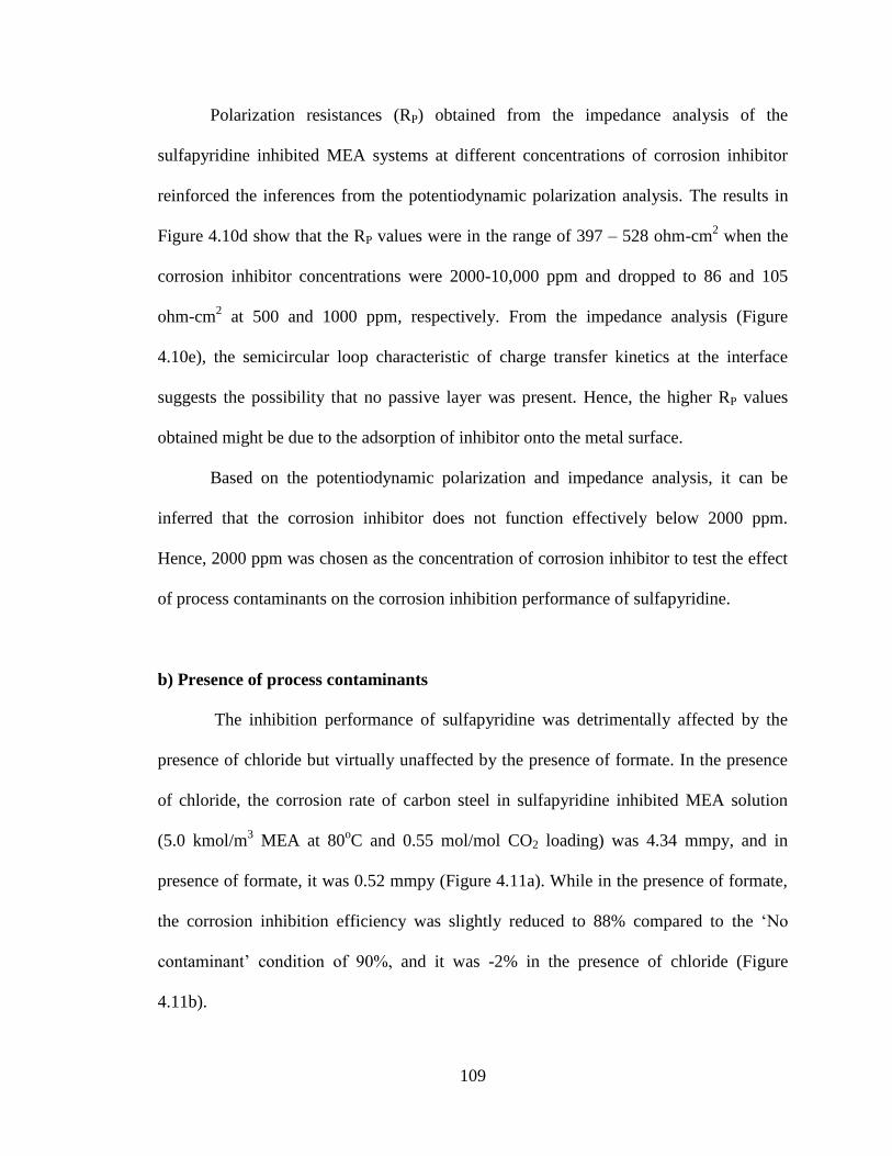
109

Polarization resistances (RP) obtained from the impedance analysis of the

sulfapyridine inhibited MEA systems at different concentrations of corrosion inhibitor

reinforced the inferences from the potentiodynamic polarization analysis. The results in

Figure 4.10d show that the RP values were in the range of 397 – 528 ohm-cm2 when the

corrosion inhibitor concentrations were 2000-10,000 ppm and dropped to 86 and 105

ohm-cm2 at 500 and 1000 ppm, respectively. From the impedance analysis (Figure

4.10e), the semicircular loop characteristic of charge transfer kinetics at the interface

suggests the possibility that no passive layer was present. Hence, the higher RP values

obtained might be due to the adsorption of inhibitor onto the metal surface.

Based on the potentiodynamic polarization and impedance analysis, it can be

inferred that the corrosion inhibitor does not function effectively below 2000 ppm.

Hence, 2000 ppm was chosen as the concentration of corrosion inhibitor to test the effect

of process contaminants on the corrosion inhibition performance of sulfapyridine.


The inhibition performance of sulfapyridine was detrimentally affected by the

presence of chloride but virtually unaffected by the presence of formate. In the presence

of chloride, the corrosion rate of carbon steel in sulfapyridine inhibited MEA solution

(5.0 kmol/m3 MEA at 80

oC and 0.55 mol/mol CO2 loading) was 4.34 mmpy, and in

presence of formate, it was 0.52 mmpy (Figure 4.11a). While in the presence of formate,

the corrosion inhibition efficiency was slightly reduced to 88% compared to the ‘No

contaminant’ condition of 90%, and it was -2% in the presence of chloride (Figure

4.11b).

110

(a) (b)

(c) (d)

(e)



oC, 0.55 mol/mol CO2 loading, 2000 ppm

sulfapyridine) (a) Comparison of corrosion rate (b) Comparison of inhibition efficiencies

(c) Polarization behaviour (d) Comparison of polarization resistance (e) Impedance

behaviour

0.00

2.00

4.00

6.00


chloride formate

Co

rosi

on r

ate

(m

mp

y)


-25%

0%

25%

50%

75%

100%


chloride formate

Inh

ibit

ion

eff

icie

ncy

(%

)


-1.10

-0.90

-0.70

-0.50

-7 -6 -5 -4 -3 -2

Po

ten

tial

(V

vs

Ag/A

gC

l)


No process contaminant formate chloride

0

150

300

450

600


chloride formate

RP

(oh

m-c

m2)


0

40

80

120

160

200

0 100 200 300 400 500

Z' (

oh

m-c

m2)

Z' (ohm-cm2)No process contaminant formate chloride

111

From the potentiodynamic polarization analysis (Figure 4.11c), it can be observed that in

the presence of chloride, both the cathodic and anodic current densities were higher than

the ‘No contaminant’ condition but were almost comparable in the case of formate. This

suggests that the adsorption of inhibitor onto the metal surface was drastically affected by

the presence of chloride. No pitting tendency was induced by the presence of process

contaminants.

From Figure 4.11d, it can be observed that in the presence of formate, RP was

lower than the ‘No contaminant’ condition, but in the presence of chloride, RP was almost

as low as in the uninhibited condition. From the impedance analysis in the presence of

chloride and formate (Figure 4.11e), a semicircular loop was obtained, which is

characteristic of a capacitive loop due to charge transfer kinetics at the interface. Thus,

the reduction in the RP value in the presence of process contaminants suggests that the

adsorption of sulfapyridine molecules onto the metal surface was disrupted, and the effect

was more pronounced in the presence of chloride.

4.1.2.5 Sulfanilamide (Absence of process contaminants)

The corrosion rates of carbon steel in sulfanilamide inhibited MEA systems (5.0

kmol/m3 MEA at 80

oC, 0.55 mol/mol CO2 loading and no process contaminant) were

2.50 mmpy and 3.41 mmpy (Figure 4.12a) when the corrosion inhibitor concentrations

were 3000 and 10,000 ppm, respectively, with corresponding corrosion inhibition

efficiencies of 42% and 20% (Figure 4.12b). From the potentiodynamic polarization

analyses (Figure 4.12c), it can be observed that the metal underwent active corrosion.

112

(a) (b)

(c) (d)

(e)

Figure 4.12 Corrosion behaviour of ‘sulfanilamide’ inhibited MEA solutions (5.0

kmol/m3 MEA, 80

oC, 0.55 mol/mol CO2 loading, no process contaminant) (a)

Comparison of corrosion rate (b) Comparison of inhibition efficiencies (c) Polarization


0.00

1.00

2.00

3.00

4.00

5.00

0 3000 10000

Co

rosi

on r

ate

(m

mp

y)


Sulfanilamide

0%

25%

50%

75%

100%

3000 10000

Inh

ibit

ion

eff

icie

ncy

(%

)


Sulfanilamide

-1.10

-0.90

-0.70

-0.50

-6 -5 -4 -3 -2

Po

ten

tial

(V

vs

Ag/A

gC

l


uninhibited 3000 ppm 10000 ppm

0

60

120

0 3000 10000

Rp(o

hm

-cm

2)


Sulfanilamide

0

20

40

0 60 120

Z''

(oh

m-c

m2)

Z' (ohm-cm2)


113

Compared to the uninhibited condition, the cathodic current densities were lower in the

case of 3000 ppm and almost similar in the case of 10,000 ppm (Figure 4.12c). No pitting

tendency was induced by the presence of inhibitor at any concentration.

The polarization resistances (RP) obtained from the impedance analysis were 104

and 84 ohm-cm2 at corrosion inhibitor concentrations of 3000 and 10,000 ppm,

respectively, compared to the uninhibited RP value of 72 ohm-cm2 (Figure 4.12d).

Impedance analysis in the presence of inhibitor at 3000 and 10,000 ppm (Figure 4.12e)

traced a semicircle (a capacitive loop due to charge transfer kinetics) similar to that of the

uninhibited system, suggesting that no passive film might be present. Thus, the small

increase in the RP value in the presence of inhibitor might be due to the adsorption of

inhibitor molecules onto the metal surface, but as the corrosion inhibition efficiencies at

the measured concentrations were relatively poor in comparison with other inhibitors,

sulfanilamide was not tested further for the effect of its concentration and the effect of

process contaminants.

4.1.2.6 Sulfolane


Corrosion rates of carbon steel in sulfolane inhibited MEA system (5 kmol/m3

MEA at 80oC, 0.55 mol/mol CO2 loading and no process contaminant) were in the range

of 0.43 – 0.62 mmpy when the inhibitor concentrations were in the range of 2000-10,000

ppm (Figure 4.13a). At an inhibitor concentration of 1000 ppm, the corrosion rate was

3.63 mmpy, which is only slightly lower than the uninhibited corrosion rate of 4.27

mmpy. Corrosion inhibition efficiency was in the range of 85 – 90 % when the corrosion

114

(a) (b)

(c) (d)

(e)

Figure 4.13 Corrosion behaviour of ‘sulfolane’ inhibited MEA solutions (5.0 kmol/m3

MEA, 80oC, 0.55 mol/mol CO2 loading, no process contaminant) (a) Comparison of

corrosion rate (b) Comparison of inhibition efficiencies (c) Polarization behaviour (d)

Comparison of polarization resistance (e) Impedance behaviour

0.00

1.00

2.00

3.00

4.00

5.00

0 1000 2000 3000 5000 10000

Co

rosi

on r

ate

(m

mp

y)


sulfolane

0%

25%

50%

75%

100%

1000 2000 3000 5000 10000

Inh

ibit

ion

eff

icie

ncy

(%

)


sulfolane

-1.10

-0.90

-0.70

-0.50

-6 -5 -4 -3 -2

Po

ten

tial

(V

vs

Ag/A

gC

l)


Uninhibited 1000 ppm 2000 ppm

3000 ppm 5000 ppm 10000 ppm

0

100

200

300

400

500

0 1000 2000 3000 5000 10000

RP

(oh

m-c

m2)


sulfolane

0

30

60

90

120

150

180

0 150 300 450

Z''

(oh

m-c

m2)

Z' (ohm-cm2)

Uninhibited 1000 ppm 2000 ppm3000 ppm 5000 ppm 10000 ppm

115

inhibitor concentrations were in the range of 2000-10,000 ppm, which dropped to 15% at

1000 ppm (Figure 4.13b). This suggested that the minimum concentration required for

effective corrosion inhibition was 2000 ppm. However, no specific trend was observed

between corrosion rate and concentration of corrosion inhibitor above 2000 ppm. From

the potentiodynamic polarization behaviour (Figure 4.13c), it can be observed that when

the corrosion inhibitor concentration was 1000 ppm, the cathodic and anodic current

densities were close to the uninhibited condition, but at higher concentrations (2000 -

10000 ppm), the cathodic current densities were lower. This suggests that the presence of

corrosion inhibitor impeded the cathodic reaction when the inhibitor concentration was

2000 – 10,000 ppm. As the metal was in an active state, the decrease in corrosion rate

might be due to the adsorption of sulfolane molecules onto the metal surface. No pitting

tendency was induced by the presence of sulfolane at any concentration.

Polarization resistances (RP) obtained from the impedance analysis reinforced the

observation from the potentiodynamic polarization analysis. When the concentration of

corrosion inhibitors was in the range of 2000 – 10,000 ppm, higher RP values (331– 445

ohm-cm2) were obtained, but at 1000 ppm, it dropped to 116 ohm-cm

2. An approximate

linear trend between concentration of corrosion inhibitor and RP value was observed

(Figure 4.13d). From the impedance analysis (Figure 4.13e), the semicircular loop

characteristic of charge transfer kinetics at the metal/solution interface suggests that no

passive layer might be present. Hence, the increase in RP might be due to the adsorption

of inhibitor molecules onto the metal surface. An inhibitor concentration of 2000 ppm,

below which the corrosion inhibition was not effective, was chosen for testing the effect

of process contaminants on the inhibition performance of sulfolane.

116


The inhibition performance of sulfolane was not affected by the presence of

chloride or formate. The corrosion rate was 0.48 mmpy in the presence of chloride and

0.44 mmpy in the presence of formate, which was better than the corrosion rate for the

‘No contaminant’ condition, which was 0.62 mmpy (Figure 4.14a). Consequently, the

inhibition efficiencies were marginally better in the presence of chloride and formate

compared to the ‘No contaminant’ condition (Figure 4.14b). From the potentiodynamic

polarization analysis (Figure 4.14c), it was observed that anodic and cathodic current

densities in the presence of process contaminants were slightly lower than the anodic and

cathodic current densities in the absence of the process contaminants. No pitting tendency

was induced by the presence of process contaminants.

From Figure 4.14d, it can be observed that the polarization resistance (RP)

obtained from the impedance analysis was slightly lower in the presence of chloride (314

ohm-cm2) and was higher in the presence of formate (431 ohm-cm

2) compared to the ‘No

process contaminant’ condition (358 ohm-cm2). The semicircular loop obtained from the

impedance analysis (4.14e) represents a capacitive loop due to the charge transfer

kinetics at the interface. Thus, the adsorption of inhibitor molecules onto the metal

surface might be slightly affected by the presence of chloride but was enhanced by the

presence of formate.

4.1.2.7 Thiosalicylic acid (Absence of process contaminants)

Corrosion rates of carbon steel in ‘thiosalicylic acid’ inhibited MEA systems (5.0

kmol/m3 MEA at 80


117

(a) (b)

(a) (d)

(e)



oC, 0.55 mol/mol CO2 loading, 2000 ppm sulfolane)



0.00

2.00

4.00

6.00


chloride formate

Co

rosi

on r

ate

(m

mp

y)


0%

25%

50%

75%

100%


chloride formate

Inh

ibit

ion

eff

icie

ncy

(%

)


-1.10

-0.90

-0.70

-0.50

-6 -5 -4 -3 -2

Po

ten

tial

(V

vs

Ag/A

gC

l)



0

150

300

450


chloride formate

RP

(oh

m-c

m2)


0

30

60

90

120

150

180

0 100 200 300 400 500

Z''

(oh

m-c

m2)

Z' (ohm-cm2)


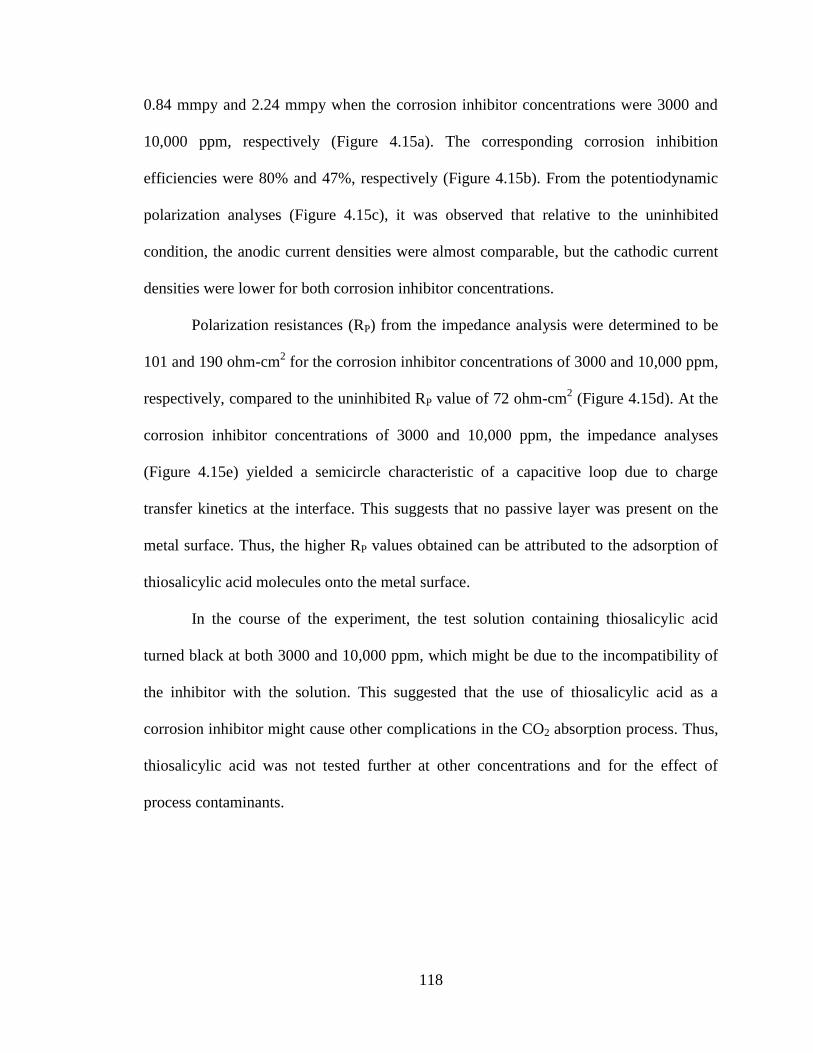
118

0.84 mmpy and 2.24 mmpy when the corrosion inhibitor concentrations were 3000 and

10,000 ppm, respectively (Figure 4.15a). The corresponding corrosion inhibition

efficiencies were 80% and 47%, respectively (Figure 4.15b). From the potentiodynamic

polarization analyses (Figure 4.15c), it was observed that relative to the uninhibited

condition, the anodic current densities were almost comparable, but the cathodic current

densities were lower for both corrosion inhibitor concentrations.

Polarization resistances (RP) from the impedance analysis were determined to be

101 and 190 ohm-cm2 for the corrosion inhibitor concentrations of 3000 and 10,000 ppm,

respectively, compared to the uninhibited RP value of 72 ohm-cm2 (Figure 4.15d). At the

corrosion inhibitor concentrations of 3000 and 10,000 ppm, the impedance analyses

(Figure 4.15e) yielded a semicircle characteristic of a capacitive loop due to charge

transfer kinetics at the interface. This suggests that no passive layer was present on the

metal surface. Thus, the higher RP values obtained can be attributed to the adsorption of

thiosalicylic acid molecules onto the metal surface.

In the course of the experiment, the test solution containing thiosalicylic acid

turned black at both 3000 and 10,000 ppm, which might be due to the incompatibility of

the inhibitor with the solution. This suggested that the use of thiosalicylic acid as a

corrosion inhibitor might cause other complications in the CO2 absorption process. Thus,

thiosalicylic acid was not tested further at other concentrations and for the effect of

process contaminants.

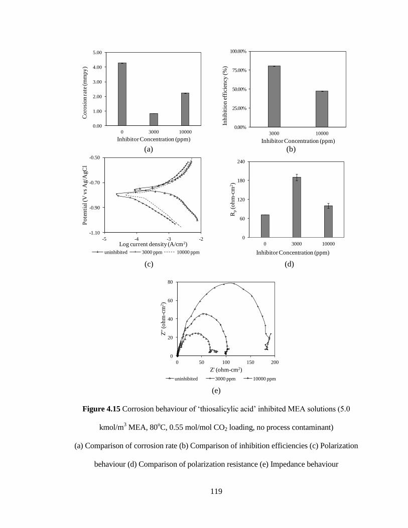
119

(a) (b)

(c) (d)

(e)

Figure 4.15 Corrosion behaviour of ‘thiosalicylic acid’ inhibited MEA solutions (5.0

kmol/m3 MEA, 80




0.00

1.00

2.00

3.00

4.00

5.00

0 3000 10000

Co

rosi

on r

ate

(m

mp

y)


Thiosalicylic acid

0.00%

25.00%

50.00%

75.00%

100.00%

3000 10000

Inh

ibit

ion

eff

icie

ncy

(%

)


-1.10

-0.90

-0.70

-0.50

-5 -4 -3 -2

Po

ten

tial

(V

vs

Ag/A

gC

l



0

60

120

180

240

0 3000 10000

Rp(o

hm

-cm

2)


Thiosalicylic acid

0

20

40

60

80

0 50 100 150 200

Z''

(oh

m-c

m2)

Z' (ohm-cm2)


120

4.1.2.8 Sodium thiosulfate


Corrosion rates of carbon steel in the sodium thiosulfate inhibited MEA systems

(5.0 kmol/m3 MEA at 80


in the range of 0.26 - 0.38 mmpy when the corrosion inhibitor concentrations were 250 –

10,000 ppm (Figure 4.16a) with corresponding corrosion inhibition efficiencies of 91-

94% (Figure 4.16b). From the potentiodynamic polarization analysis (Figure 4.17a), two

different behaviours, depending on the concentration of corrosion inhibitor, were

observed. When the corrosion inhibitor concentration was 250 or 500 ppm, the metal was

in an active state. The anodic current densities were higher and the cathodic current

densities were lower than the uninhibited condition. However, at higher corrosion

inhibitor concentrations (1000 – 10,000 ppm), the metal showed passivation tendency

(Figure 4.17a), but the passive layer was weak and unstable. From the anodic polarization

curves, it can be observed that as the initial passive layer broke down, an increase in

anodic current densities was observed. This was followed by a repassivation and lower

current densities, and this cycle repeated until a stable passive layer was formed.

Formation of a thin black film over the metal surface (Figure 4.17b) was observed, which

might be due to the adsorption of thiosulfate (S2O32-

) ions. The corrosion inhibition was

anodic in nature. Though no trend between corrosion rate and corrosion inhibitor

concentration was found, the passive behaviour was observed only at 1000 ppm and

above. No pitting tendency was induced by the presence of inhibitor at any concentration.

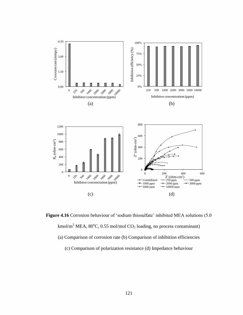
121

(a) (b)

(c) (d)

Figure 4.16 Corrosion behaviour of ‘sodium thiosulfate’ inhibited MEA solutions (5.0

kmol/m3 MEA, 80


(a) Comparison of corrosion rate (b) Comparison of inhibition efficiencies

(c) Comparison of polarization resistance (d) Impedance behaviour

0.00

1.50

3.00

4.50

Co

rosi

on r

ate

(m

mp

y)


thiosulfate

0%

25%

50%

75%

100%

250 500 1000 2000 3000 5000 10000

Inh

ibit

ion

eff

icie

ncy

(%

)


thiosulfate

0

200

400

600

800

1000

1200

RP

(oh

m-c

m2)

Inhibitor concentration (ppm)thiosulfate

0

200

400

600

800

0 200 400 600

Z''

(oh

m-c

m2)

Z' (ohm-cm2)Uninhibited 250 ppm 500 ppm1000 ppm 2000 ppm 3000 ppm5000 ppm 10000 ppm

122

(a)

(b)

Figure 4.17 (a) Polarization behaviour of ‘sodium thiosulfate’ inhibited MEA solutions



(b) Working electrode after stable open circuit potential in presence of sodium thiosulfate


oC, 0.55 mol/mol CO2 loading and 1000 ppm sodium thiosulfate)

(Original in colour)

-1.20

-0.90

-0.60

-0.30

0.00

0.30

0.60

0.90

-7 -6 -5 -4 -3 -2

Po

ten

tial

(V

vs

Ag/A

gC

l)


0 ppm 250 ppm 500 ppm

1000 ppm 2000 ppm 3000ppm

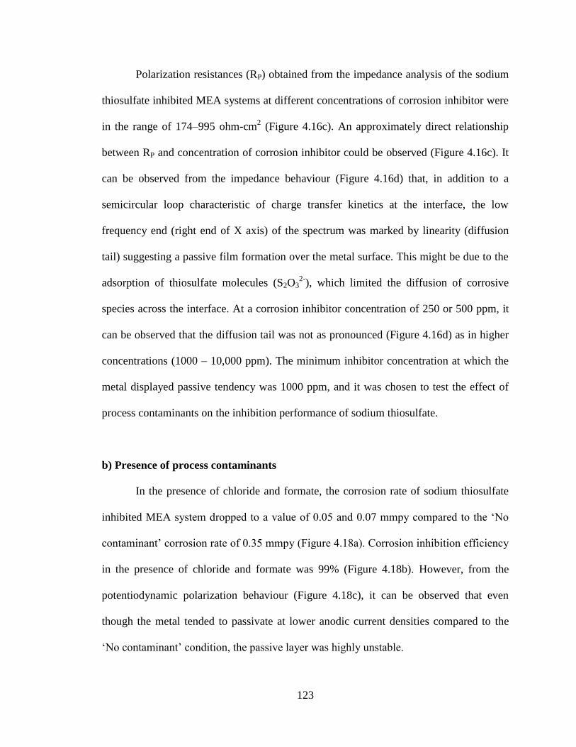
123

Polarization resistances (RP) obtained from the impedance analysis of the sodium

thiosulfate inhibited MEA systems at different concentrations of corrosion inhibitor were

in the range of 174–995 ohm-cm2 (Figure 4.16c). An approximately direct relationship

between RP and concentration of corrosion inhibitor could be observed (Figure 4.16c). It

can be observed from the impedance behaviour (Figure 4.16d) that, in addition to a

semicircular loop characteristic of charge transfer kinetics at the interface, the low

frequency end (right end of X axis) of the spectrum was marked by linearity (diffusion

tail) suggesting a passive film formation over the metal surface. This might be due to the

adsorption of thiosulfate molecules (S2O32-

), which limited the diffusion of corrosive

species across the interface. At a corrosion inhibitor concentration of 250 or 500 ppm, it

can be observed that the diffusion tail was not as pronounced (Figure 4.16d) as in higher

concentrations (1000 – 10,000 ppm). The minimum inhibitor concentration at which the

metal displayed passive tendency was 1000 ppm, and it was chosen to test the effect of

process contaminants on the inhibition performance of sodium thiosulfate.


In the presence of chloride and formate, the corrosion rate of sodium thiosulfate

inhibited MEA system dropped to a value of 0.05 and 0.07 mmpy compared to the ‘No

contaminant’ corrosion rate of 0.35 mmpy (Figure 4.18a). Corrosion inhibition efficiency

in the presence of chloride and formate was 99% (Figure 4.18b). However, from the

potentiodynamic polarization behaviour (Figure 4.18c), it can be observed that even

though the metal tended to passivate at lower anodic current densities compared to the

‘No contaminant’ condition, the passive layer was highly unstable.

124

(a) (b)

(c) (d)

(e)



oC, 0.55 mol/mol CO2 loading, 1000 ppm sodium

thiosulfate) (a) Comparison of corrosion rate (b) Comparison of inhibition efficiencies (c)

Polarization behaviour (d) Comparison of polarization resistance (e) Impedance behaviour

0.00

2.00

4.00

6.00


chloride formate

Co

rosi

on r

ate

(m

mp

y)


0%

25%

50%

75%

100%


chloride formate

Inh

ibit

ion

eff

icie

ncy

(%

)


-1.20

-0.90

-0.60

-0.30

0.00

0.30

0.60

0.90

-7 -6 -5 -4 -3 -2

Po

ten

tial

(V

vs

Ag/A

gC

l)



0

200

400

600

800

1000


chloride formate

RP

(oh

m-c

m2)


0

100

200

300

400

0 100 200 300 400 500

Z''

(oh

m-c

m2)

Z' (ohm-cm2)

No contaminant formate chloride

125

As the initial passive layer broke down, an increase in anodic current densities was

observed, which was followed by repassivation. This cycle repeated without the

formation of a stable passive layer throughout the anodic polarization, suggesting that the

passive layer might not be protective in the presence of process contaminant. No pitting

tendency was induced by the presence of process contaminants.

Polarization resistances (RP) obtained from the impedance analysis in the

presence of chloride and formate were 889 and 974 ohm-cm2, respectively, which was

higher than the ‘No contaminant’ condition (594 ohm-cm2) (Figure 4.18d). This was in

agreement with the lower corrosion rates obtained from potentiodynamic polarization

analysis. Impedance behaviour (Figure 4.18e) in the presence and absence of the process

contaminants was similar in terms of trends characterized by the presence of a diffusion

tail suggesting that the metal was in a passive state. The unstable nature of the passive

layer in the presence of process contaminants could not be predicted, mainly because the

impedance analysis is carried out at the equilibrium potential of the metal unlike

potentiodynamic polarization.

126

4.1.3 Comparison of corrosion inhibition performance of different inhibitors

Corrosion inhibition performance of different corrosion inhibitors was compared

based on the corrosion rates obtained for each case (Figure 4.19a). Corrosion rates at the

inhibitor concentration at which the effect of process contaminants was tested in each

case were chosen as the basis for comparison. In the case of sulfanilamide and

thiosalicylic acid, for which the effects of process contaminants were not tested, the

corrosion inhibitor concentration corresponding to the lowest corrosion rate was chosen.

In the absence of process contaminants, corrosion rates for different corrosion

inhibitors were in the range of 0.35 to 2.50 mmpy compared to the uninhibited corrosion

rate of 4.27 mmpy. The lowest corrosion rate was observed for sodium thiosulfate and the

highest corrosion rate was obtained for sulfanilamide. In the absence of process

contaminants, the corrosion rate decreased in the following order: sulfanilamide >

thiosalicylic acid > sulfolane > 2-aminobenzene sulfonic acid > 3-aminobenzene sulfonic

acid > 4-aminobenzene sulfonic acid > sulfapyridine > sodium thiosulfate.

In presence of chloride, the corrosion rate of 3-amino benzene sulfonic acid

increased to 1.65 mmpy from 0.48 mmpy, whereas in case of sulfapyridine, the corrosion

rate increased to 4.34 mmpy from 0.44 mmpy. For 4-aminobenzene sulfonic acid,

sulfolane and sodium thiosulfate, the corrosion rate was lower than the ‘No contaminant’

condition, and in the case of 2-aminobenzene sulfonic acid, the corrosion rate was

slightly higher. In the presence of chloride, the corrosion rate decreased in the following

order: sulfapyridine > 3-aminobenzene sulfonic acid > 2-aminobenzene sulfonic acid >

sulfolane > 4-aminobenzene sulfonic acid > sodium thiosulfate.

127

(a) (b)

(c)



oC, 0.55 mol/mol CO2 loading) (a) Comparison of

corrosion rate (b) Comparison of polarization resistance (c) Comparison of inhibition

efficiencies

0.00

1.00

2.00

3.00

4.00

5.00

6.00

2-a

min

ob

enze

ne

sulf

on

ic a

cid

3-a

min

ob

enze

ne

sulf

on

ic a

cid

4-a

min

ob

enze

ne

sulf

on

ic a

cid

sulf

ap

yri

din

e

sulf

an

ilam

ide

sulf

ola

ne

thio

sali

cyli

c aci

d

thio

sulf

ate

Co

rosi

on r

ate

(m

mp

y)


0

200

400

600

800

1000

2-a

min

ob

enze

ne

sulf

on

ic a

cid

3-a

min

ob

enze

ne

sulf

on

ic a

cid

4-a

min

ob

enze

ne

sulf

on

ic a

cid

sulf

ap

yri

din

e

sulf

an

ilam

ide

sulf

ola

ne

thio

sali

cyli

c aci

d

thio

sulf

ate

RP

(oh

m-c

m2)


-40%

-20%

0%

20%

40%

60%

80%

100%

Inh

ibit

ion

eff

icie

ncy

(%

)


128

In the presence of formate, 2-aminobenzene sulfonic acid, 3-aminobenzene

sulfonic acid, and 4-aminobenzene sulfonic acid had increased corrosion rates higher than

the uninhibited condition. For sulfapyridine, the corrosion rate was slightly higher than

the ‘No contaminant’ condition, whereas in the case of sulfolane and sodium thiosulfate,

lower corrosion rates were observed. In the presence of formate, the corrosion rate

decreased in the following order: 2-aminobenzene sulfonic acid > 3-aminobenzene

sulfonic acid > 4-aminobenzene sulfonic acid > sulfapyridine > sulfolane > sodium

thiosulfate.

Similarly, polarization resistances (RP) obtained from impedance analysis for

different corrosion inhibitors can also be used to compare the corrosion inhibition

performance (Figure 4.19b). The results were in agreement with the inferences of the

corrosion rate comparison. In the absence of process contaminants, RP decreases in the

following order: sodium thiosulfate > sulfapyridine > 4-aminobenzene sulfonic acid > 2-

aminobenzene sulfonic acid > 3-aminobenzene sulfonic acid > sulfolane > thiosalicylic

acid > sulfanilamide. In presence of chloride, RP decreased in the following order:

sodium thiosulfate > 4-aminobenzene sulfonic acid > 2-aminobenzene sulfonic acid >

sulfolane > sulfapyridine > 3-aminobenzene sulfonic acid. In the presence of formate,

the RP decreased in the following order: sodium thiosulfate > sulfolane > sulfapyridine >

3-aminobenzene sulfonic acid > 4-aminobenzene sulfonic acid > 2-aminobenzene

sulfonic acid. From Figure 4.19c, it can be observed that in the absence of process

contaminants, the corrosion inhibition efficiencies were in the range of 42 to 92%. The

lowest corrosion inhibition efficiency was obtained for sulfanilamide, whereas the

highest efficiency was observed in the case of sodium thiosulfate.

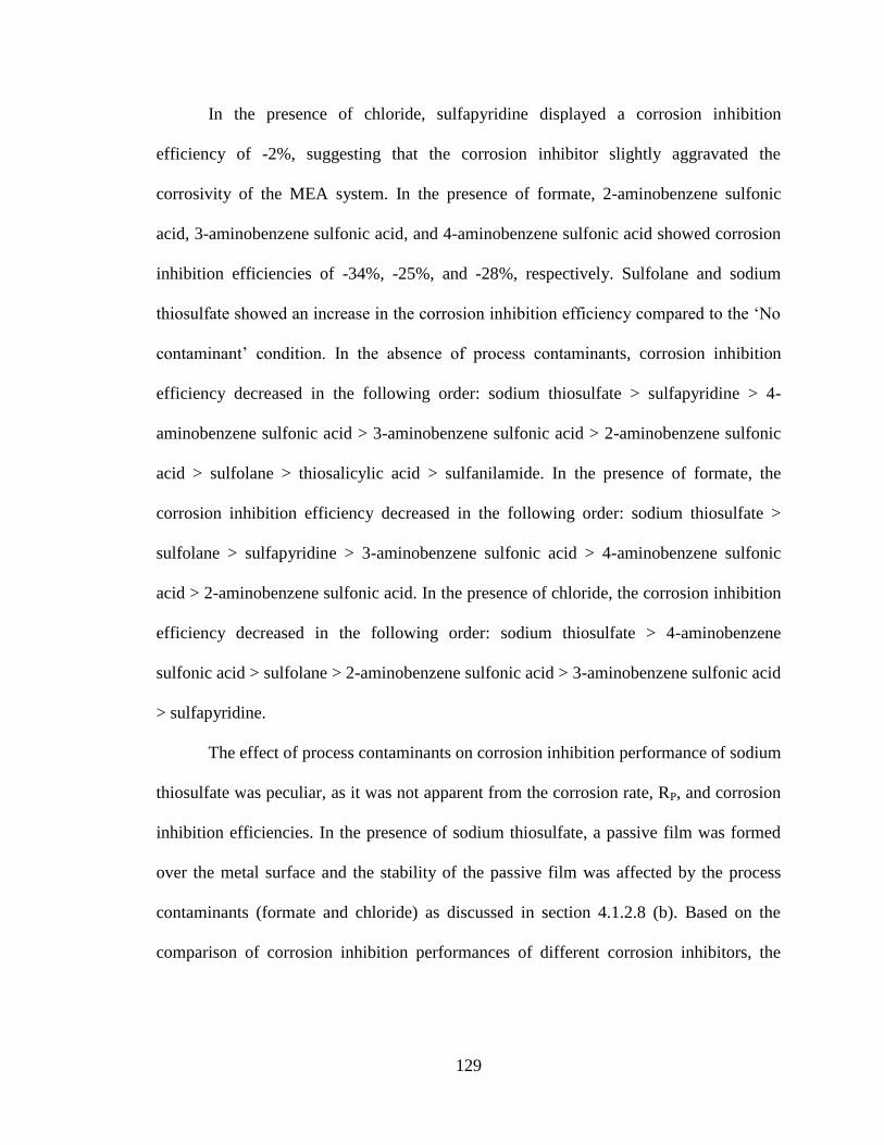
129

In the presence of chloride, sulfapyridine displayed a corrosion inhibition

efficiency of -2%, suggesting that the corrosion inhibitor slightly aggravated the

corrosivity of the MEA system. In the presence of formate, 2-aminobenzene sulfonic

acid, 3-aminobenzene sulfonic acid, and 4-aminobenzene sulfonic acid showed corrosion

inhibition efficiencies of -34%, -25%, and -28%, respectively. Sulfolane and sodium

thiosulfate showed an increase in the corrosion inhibition efficiency compared to the ‘No

contaminant’ condition. In the absence of process contaminants, corrosion inhibition

efficiency decreased in the following order: sodium thiosulfate > sulfapyridine > 4-

aminobenzene sulfonic acid > 3-aminobenzene sulfonic acid > 2-aminobenzene sulfonic

acid > sulfolane > thiosalicylic acid > sulfanilamide. In the presence of formate, the

corrosion inhibition efficiency decreased in the following order: sodium thiosulfate >

sulfolane > sulfapyridine > 3-aminobenzene sulfonic acid > 4-aminobenzene sulfonic

acid > 2-aminobenzene sulfonic acid. In the presence of chloride, the corrosion inhibition

efficiency decreased in the following order: sodium thiosulfate > 4-aminobenzene

sulfonic acid > sulfolane > 2-aminobenzene sulfonic acid > 3-aminobenzene sulfonic acid

> sulfapyridine.

The effect of process contaminants on corrosion inhibition performance of sodium

thiosulfate was peculiar, as it was not apparent from the corrosion rate, RP, and corrosion

inhibition efficiencies. In the presence of sodium thiosulfate, a passive film was formed

over the metal surface and the stability of the passive film was affected by the process

contaminants (formate and chloride) as discussed in section 4.1.2.8 (b). Based on the

comparison of corrosion inhibition performances of different corrosion inhibitors, the

130

following compounds were considered for the weight loss testing: 4-aminobenzene

sulfonic acid, sulfapyridine, sulfolane, and sodium thiosulfate.

4.2 Weight loss tests

From the weight loss values of the carbon steel specimens withdrawn at regular

time intervals from the weight loss tests, the corrosion rates were determined. In order to

analyze the nature of the corrosion product formed in each case, the specimens tested for

the longest duration (28 days) were subjected to surface analytical testing such as

Scanning Electron Microscopy (SEM), Energy Dispersive X-Ray Spectroscopy (EDS),

and X-Ray Diffraction (XRD).

4.2.1 Corrosion behaviour of uninhibited MEA systems

The corrosion rate of carbon steel in uninhibited MEA solution (5.0 kmol/m3

MEA, 80oC, 0.55 mol/mol CO2 loading and No process contaminant) after 28 days was

0.50 mmpy (Table 4.3). From Figure 4.20, for the uninhibited condition, it can be

observed that a steep increase in corrosion rate after 7 days was followed by a gradual

increase until it reached a steady value after 21 days (0.50 mmpy). The final corrosion

rate of 0.50 mmpy was lower than the electrochemical corrosion rate of carbon steel in an

uninhibited MEA system, which was 4.27 mmpy. This might be due to the formation of a

stable corrosion product as a result of longer exposure time, which might act as a barrier

between the metal and the solution. From the SEM images (Figure 4.21a), a uniform

corrosion product formed over the metal surface can be clearly seen. From the EDS

analysis (4.21b), a significant increase in the amounts of oxygen and carbon in the tested

131

Table 4.3 Summary of weight loss experimental results

Experimental

condition

Corrosion rate (mmpy) I.E (after

28 days)

(%)

pH σ

(mS/cm) 7 days 14 days 21 days 28 days

Uninhibited 0.39 0.46 0.50 0.50 - 8.34 38.97

4-aminobenzene

sulfonic acid - 0.69 0.68 0.77 -54.81 8.38 39.09

Sulfapyridine 0.24 0.18 0.19 0.23 54.72 8.33 42.30

Sulfolane 0.34 0.30 0.28 0.28 44.26 8.32 41.27

Thiosulfate 0.44 0.43 0.48 0.45 10.62 8.31 42.66

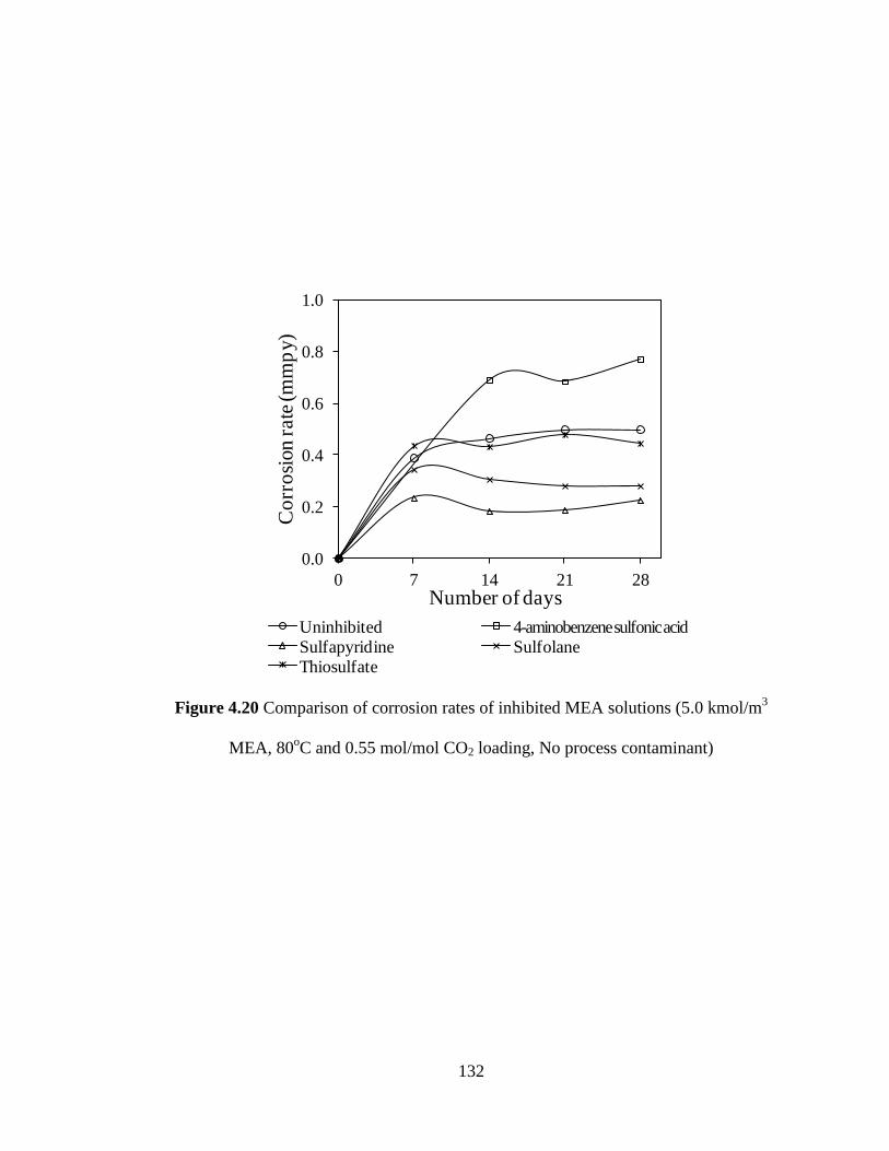
132

Figure 4.20 Comparison of corrosion rates of inhibited MEA solutions (5.0 kmol/m

3

MEA, 80oC and 0.55 mol/mol CO2 loading, No process contaminant)

0.0

0.2

0.4

0.6

0.8

1.0

0 7 14 21 28

Co

rro

sion

rate

(m

mp

y)

Number of days

Uninhibited 4-aminobenzene sulfonic acid

Sulfapyridine SulfolaneThiosulfate

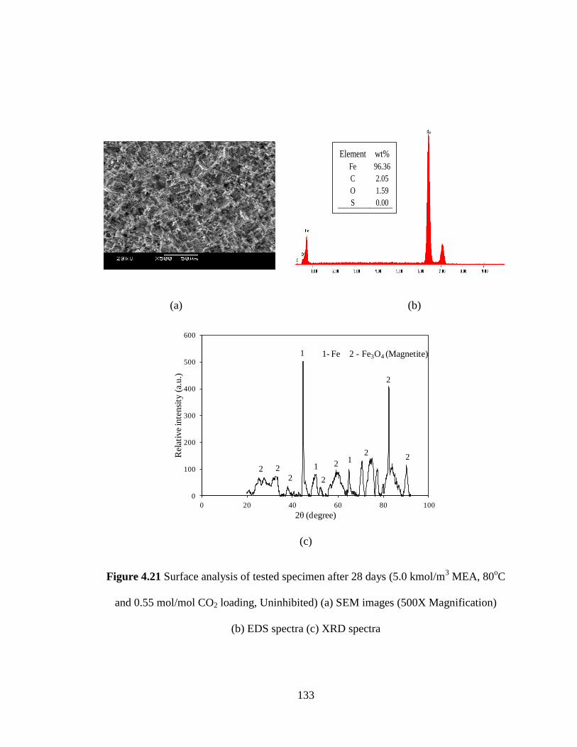
133

(a) (b)

(c)

Figure 4.21 Surface analysis of tested specimen after 28 days (5.0 kmol/m3 MEA, 80

oC

and 0.55 mol/mol CO2 loading, Uninhibited) (a) SEM images (500X Magnification)

(b) EDS spectra (c) XRD spectra

Element wt%

Fe 96.36

C 2.05

O 1.59

S 0.00

0

100

200

300

400

500

600

0 20 40 60 80 100

Rel

ativ

e in

tensi

ty (

a.u.)

2θ (degree)

2 22

1

11

2

2

2

2

2

1- Fe 2 - Fe3O4 (Magnetite)

134

specimens compared to the fresh specimen could be observed (Figure 4.22). This might

be due to the formation of corrosion products based on carbon and oxygen. In the XRD

analysis (Figure 4.22c), the peaks obtained were broader, suggesting that the corrosion

product might be poorly crystalline. Hence, different peaks lying in proximity could

possibly have merged together to form a single broad peak, making it difficult to analyze.

Comparing the results with the reference data (ICDD) for different compounds, the

corrosion product was characterized mainly to be in the form of Fe3O4 (magnetite). In

addition to Fe3O4, peaks corresponding to iron (Fe) could also be seen, which suggests

that the surface layer is less protective. Additionally, the increase in the percent weight

of carbon suggests that the surface might also contain amorphous iron carbonate

(FeCO3).

4.2.2 Corrosion behaviour of inhibited MEA systems

For 4-aminobenzene sulfonic acid, it can be observed (Table 4.3) that the

corrosion rate after 28 days of weight loss testing was 0.77 mmpy corresponding to an

aggravation of corrosion by about 55% (Figure 4.20). From electrochemical testing, it

was observed that the corrosion inhibitor actually increased the corrosion rate in the

presence of formate (Figure 4.9). Solution degradation products such as formate could be

formed in long-term tests and might interfere with the adsorption of the inhibitor onto the

metal surface and expose the metal. From SEM images (Figure 4.24a), it can be observed

that the uniform corrosion products over the metal surface were similar in appearance and

distribution to the uninhibited result (Figure 4.21a). From EDS analysis (Figure 4.24b),

larger quantities of oxygen and carbon than in the uninhibited condition were observed,

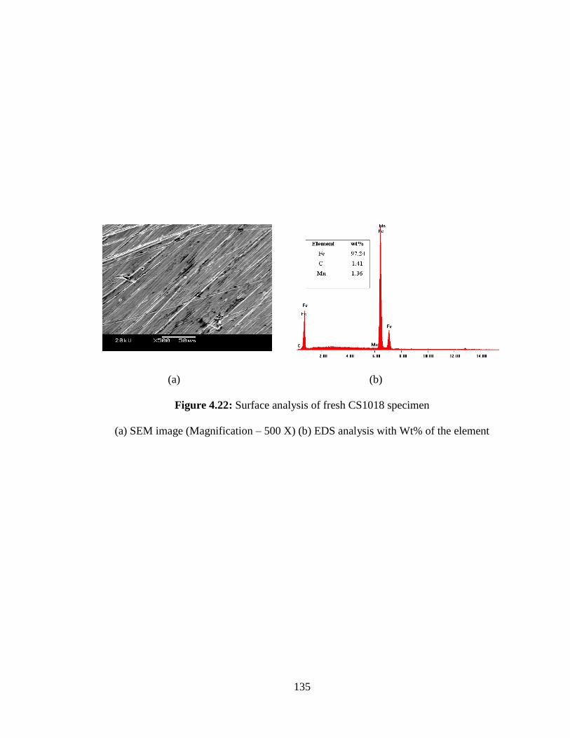
135

(a) (b)

Figure 4.22: Surface analysis of fresh CS1018 specimen

(a) SEM image (Magnification – 500 X) (b) EDS analysis with Wt% of the element

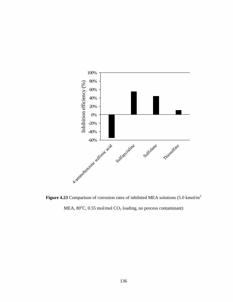
136

Figure 4.23 Comparison of corrosion rates of inhibited MEA solutions (5.0 kmol/m3

MEA, 80oC, 0.55 mol/mol CO2 loading, no process contaminant)

-60%

-40%

-20%

0%

20%

40%

60%

80%

100%

Inh

ibit

ion

eff

icie

ncy

(%

)

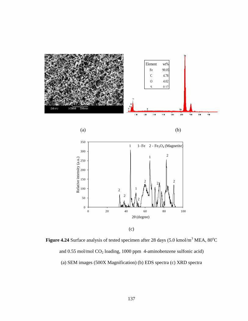
137

(a) (b)

(c)


oC

and 0.55 mol/mol CO2 loading, 1000 ppm 4-aminobenzene sulfonic acid)

(a) SEM images (500X Magnification) (b) EDS spectra (c) XRD spectra

Element wt%

Fe 90.05

C 4.78

O 4.02

S 0.17

Element wt%

Fe 90.05

C 4.78

O 4.02

S 0.17

0

50

100

150

200

250

300

350

0 20 40 60 80 100

Rel

ativ

e in

ten

sity

(a.

u.)

2θ (degree)

2

2

1

1

2

2

1

22

2


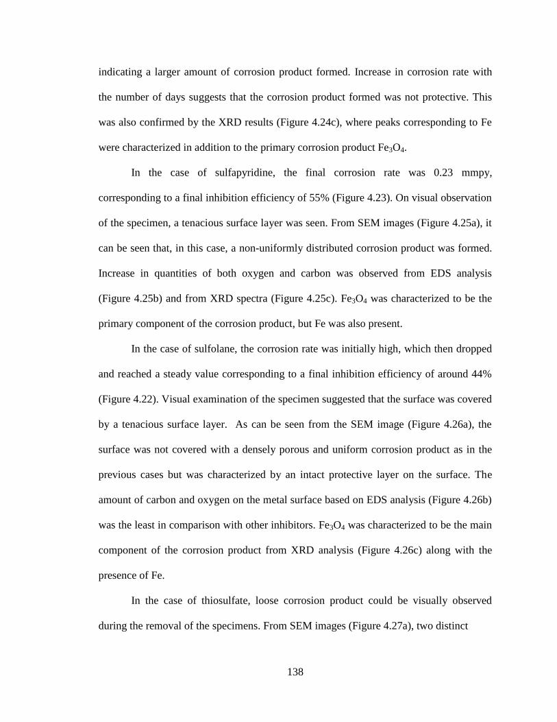
138

indicating a larger amount of corrosion product formed. Increase in corrosion rate with

the number of days suggests that the corrosion product formed was not protective. This

was also confirmed by the XRD results (Figure 4.24c), where peaks corresponding to Fe

were characterized in addition to the primary corrosion product Fe3O4.

In the case of sulfapyridine, the final corrosion rate was 0.23 mmpy,

corresponding to a final inhibition efficiency of 55% (Figure 4.23). On visual observation

of the specimen, a tenacious surface layer was seen. From SEM images (Figure 4.25a), it

can be seen that, in this case, a non-uniformly distributed corrosion product was formed.

Increase in quantities of both oxygen and carbon was observed from EDS analysis

(Figure 4.25b) and from XRD spectra (Figure 4.25c). Fe3O4 was characterized to be the

primary component of the corrosion product, but Fe was also present.

In the case of sulfolane, the corrosion rate was initially high, which then dropped

and reached a steady value corresponding to a final inhibition efficiency of around 44%

(Figure 4.22). Visual examination of the specimen suggested that the surface was covered

by a tenacious surface layer. As can be seen from the SEM image (Figure 4.26a), the

surface was not covered with a densely porous and uniform corrosion product as in the

previous cases but was characterized by an intact protective layer on the surface. The

amount of carbon and oxygen on the metal surface based on EDS analysis (Figure 4.26b)

was the least in comparison with other inhibitors. Fe3O4 was characterized to be the main

component of the corrosion product from XRD analysis (Figure 4.26c) along with the

presence of Fe.

In the case of thiosulfate, loose corrosion product could be visually observed

during the removal of the specimens. From SEM images (Figure 4.27a), two distinct

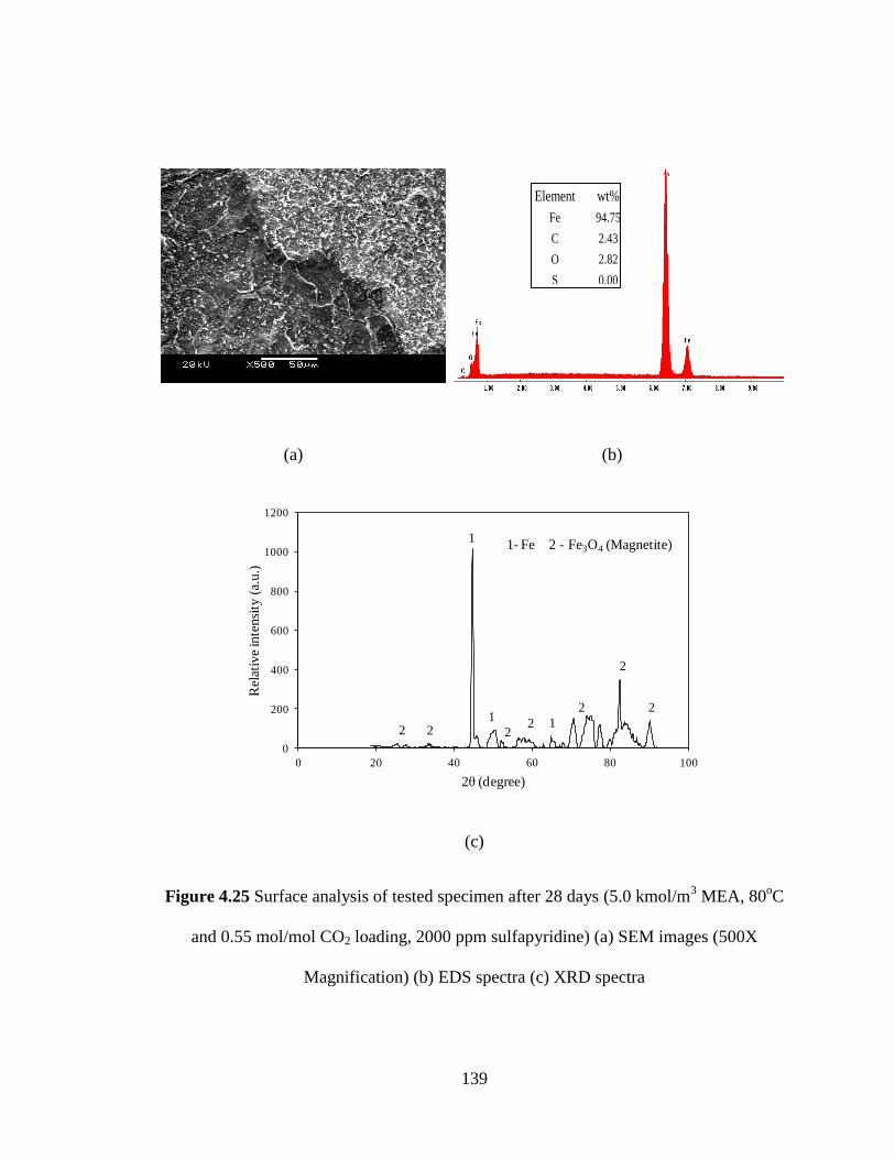
139

(a) (b)

(c)


oC

and 0.55 mol/mol CO2 loading, 2000 ppm sulfapyridine) (a) SEM images (500X

Magnification) (b) EDS spectra (c) XRD spectra

Element wt%

Fe 94.75

C 2.43

O 2.82

S 0.00

Element wt%

Fe 94.75

C 2.43

O 2.82

S 0.00

0

200

400

600

800

1000

1200

0 20 40 60 80 100

Rel

ativ

e in

ten

sity

(a.

u.)

2θ (degree)

2 2

1

1

2

2

12

2

2


140

(a) (b)

(c)


oC

and 0.55 mol/mol CO2 loading, 2000 ppm sulfolane) (a) SEM images (500X


Element wt%

Fe 96.98

C 1.68

O 1.26

S 0.10

Element wt%

Fe 96.98

C 1.68

O 1.26

S 0.10

0

50

100

150

200

250

300

350

400

0 20 40 60 80 100

Rel

ativ

e in

ten

sity

(a.

u.)

2θ (degree)

2

2

1

1

1

2

2

2

2


2

141

(a) (b)

(c)


oC

and 0.55 mol/mol CO2 loading, 1000 ppm sodium thiosulfate) (a) SEM images (500X


Element wt%

Fe 64.68

C 1.83

O 4.72

S 28.77

Element wt%

Fe 64.68

C 1.83

O 4.72

S 28.77

-20

30

80

130

180

230

280

330

380

430

0 20 40 60 80 100

Rel

ativ

e in

tensi

ty (

a.u.)

2θ (degree)

22

2

1

1

1

22

2

2

2


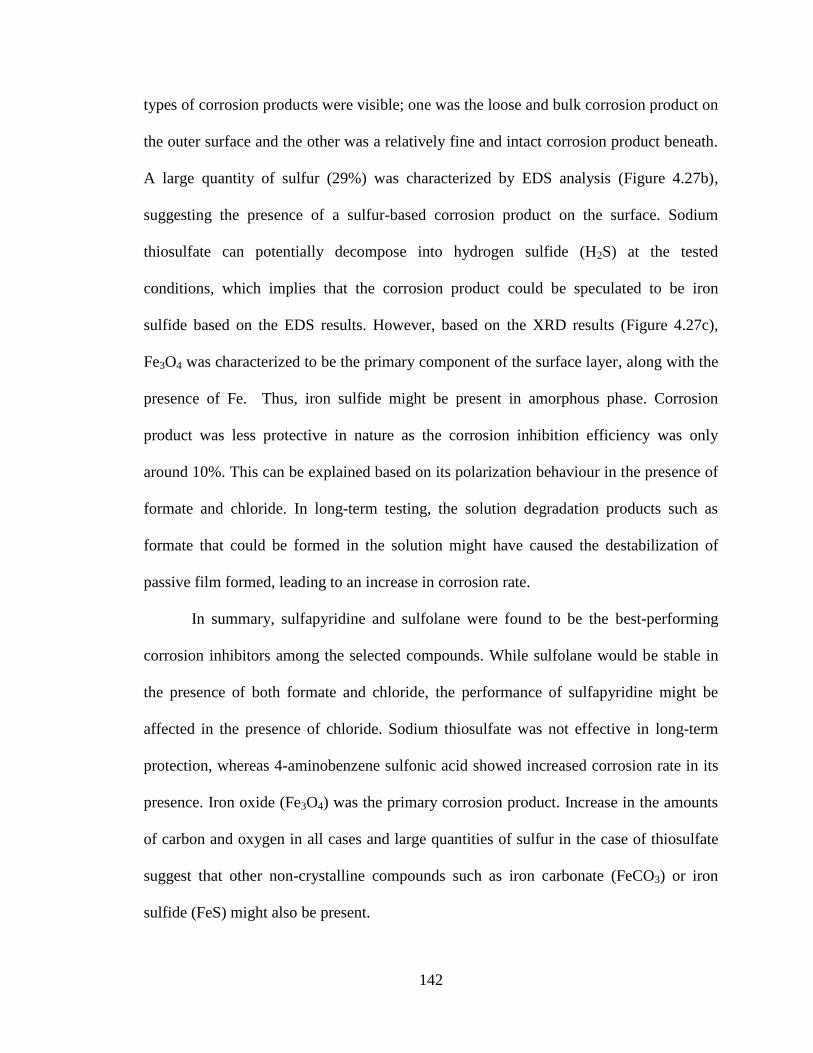
142

types of corrosion products were visible; one was the loose and bulk corrosion product on

the outer surface and the other was a relatively fine and intact corrosion product beneath.

A large quantity of sulfur (29%) was characterized by EDS analysis (Figure 4.27b),

suggesting the presence of a sulfur-based corrosion product on the surface. Sodium

thiosulfate can potentially decompose into hydrogen sulfide (H2S) at the tested

conditions, which implies that the corrosion product could be speculated to be iron

sulfide based on the EDS results. However, based on the XRD results (Figure 4.27c),

Fe3O4 was characterized to be the primary component of the surface layer, along with the

presence of Fe. Thus, iron sulfide might be present in amorphous phase. Corrosion

product was less protective in nature as the corrosion inhibition efficiency was only

around 10%. This can be explained based on its polarization behaviour in the presence of

formate and chloride. In long-term testing, the solution degradation products such as

formate that could be formed in the solution might have caused the destabilization of

passive film formed, leading to an increase in corrosion rate.

In summary, sulfapyridine and sulfolane were found to be the best-performing

corrosion inhibitors among the selected compounds. While sulfolane would be stable in

the presence of both formate and chloride, the performance of sulfapyridine might be

affected in the presence of chloride. Sodium thiosulfate was not effective in long-term

protection, whereas 4-aminobenzene sulfonic acid showed increased corrosion rate in its

presence. Iron oxide (Fe3O4) was the primary corrosion product. Increase in the amounts

of carbon and oxygen in all cases and large quantities of sulfur in the case of thiosulfate

suggest that other non-crystalline compounds such as iron carbonate (FeCO3) or iron

sulfide (FeS) might also be present.

143

5. CONCLUSIONS AND FUTURE WORK

5.1 Conclusions

Eight environmentally-friendly corrosion inhibitors were successfully chosen

based on the principle of hard and soft acids and bases (HSAB), toxicity, and quantum

chemistry for the evaluation of their corrosion inhibition performance. The important

findings of the performance evaluation are as follows:

2-aminobenzene sulfonic acid is effective, with an inhibition efficiency of 87–89% at

a concentration range of 250-3000 ppm. However, its performance can deteriorate in

the presence of formate. Corrosion inhibition is due to the adsorption of inhibitor onto

the metal surface.

3-aminobenzene sulfonic acid performs well, with an inhibition efficiency of 88-89%

at a concentration range of 250-3000 ppm. The inhibition efficiency can deteriorate in

the presence of chloride and formate. Corrosion inhibition is due to adsorption of

inhibitor on metal surface.

4-aminobenzene sulfonic acid is effective, with an inhibition efficiency of 87-91% at

a concentration range of 250-3000 ppm. Its performance can be reduced in the

presence of formate and becomes ineffective in long-term exposure. Corrosion

inhibition is due to adsorption of inhibitor onto the metal surface.

Sulfapyridine performs well, with an inhibition efficiency of 90-92% when its

concentration is at 2000 ppm or greater, but its performance can be deteriorated by

chloride. The inhibitor performance of sulfapyridine can be maintained in long-term

exposure.

144

Sulfanilamide is not an effective corrosion inhibitor, as its inhibition efficiency is 20-

42%.

Sulfolane is an effective corrosion inhibitor when its concentration is at least 2000

ppm. Its inhibition performance is unaffected by the presence of chloride and formate,

and it can be maintained during long-term exposure. Corrosion inhibition is due to the

adsorption of inhibitor on the metal surface.

Thiosalicylic acid is not an effective corrosion inhibitor, as its efficiency is 47-80%.

The presence of thiosalicylic acid causes color change of the MEA solution.

Sodium thiosulfate is an effective corrosion inhibitor in short-term exposure with an

inhibition efficiency of 91-94% at a concentration range of 250-10,000 ppm, but it

becomes ineffective in long-term. This is due to the instability of the passive film

formed. Its performance can be deteriorated by the presence of chloride and formate.

Sulfolane and sulfapyridine show promise as potential corrosion inhibitors due to

their inhibition performance in both short-term and long-term exposure and are

recommended for further evaluation.

5.1 Recommendations for future work

The corrosion inhibitors identified from this work can be further tested for their

effectiveness in the MEA-based CO2 absorption process under a wider range of operating

conditions. Further tests can include parametric effects on corrosion inhibition

performance by the presence of dissolved oxygen, solution velocity, solution temperature

(up to 120oC), and the presence of other process contaminants (sulfite, bicine, and

acetate). Flow loop tests can be conducted to simulate the effect of real flow conditions in

145

the plant on corrosion inhibition. The inhibitors that show promise in the above

mentioned tests can be evaluated for their effectiveness in other amine-based CO2

absorption processes, such as diethanolamine (DEA), 2-amino-2-methyl-1-propanol

(AMP), and piperazine (PZ).

146

REFERENCES

Aaron, D., Tsouris, C., (2005), Separation of CO2 from flue gas: a review, Separation

Science and Technology, 40, 321-348.

Anastas. P. T., Williamson. T. C., (1998), Green Chemistry: Frontiers in benign

chemical syntheses and processes, Oxford University Press, NY, USA.

Aroonwilas, A., (1996), High efficiency structured packing for CO2 absorption using 2-

Amino-2-methyl-2-propanol (AMP), M.A.Sc. Thesis, University of Regina,

Regina, Saskatchewan, Canada.

Asperger, R.G., Clouse, R.C., (1978), Quarternary salt-polyamine inhibitor for sour gas

conditioning solutions, US Patent 4100099.

Asperger, R.G., Krawczyk, L.S., Oakes, B.D., (1979), Method and composition for

inhibiting the corrosion of ferrous metals, US Patent 4143119.

Astarita. G., Savage. D. W., Bisio. A., (1983), Gas treating with chemical solvents,

John Wiley Publications, NY, USA.

ASM Handbook: Volume 13A – Corrosion: Fundamentals, Testing and Protection,

(2003), ASM International, OH, USA.

ASTM Standard G1-03, (2003), Standard practice for preparing, cleaning and

evaluating corrosion test specimens. In Annual Book of ASTM Standards;

American Society of Testing and Materials: West Conshohocken, PA.

ASTM Standard G106 – 89 (Reapproved 2010), Standard practice for verification of

algorithm and equipment for electrochemical impedance measurements, In

Annual Book of ASTM Standards; American Society of Testing and Materials:

West Conshohocken, PA.

147

ASTM Standard G5-94 (Reapproved 2004), Standard reference test method for making

potentiostatic and potentiodynamic anodic polarization measurements, In

Annual Book of ASTM Standards; American Society of Testing and Materials:

West Conshohocken, PA.

Bockris, J.O’M., Reddy, A.K.N., (2000), Modern Electrochemistry:Volume 2,

Springer, NY, USA.

Chakrabarti, A., (1984), Quantum chemical study of the corrosion inhibition of mild

steel in 6 percent (wt/wt) HCl by means of cyanoguanidine derivatives, Br.

Corros. J., 19, 124–126.

Chang, Z., Minevski, L., (2008), Polythiaether compounds and their use as corrosion

inhibitors, US Patent 7335794 B2

Clouse, R.C., Asperger, R.G., (1978), Cobalt-containing inhibitor for sour gas


Clouse, R.C., Asperger, R.G., (1978), Inhibitors for gas conditioning solutions, US

Patent 4102804.

Davidson, J.R., Friedli, H.R., (1978), Method and composition for inhibiting the

corrosion of metals, US Patent 4071470

DeHart, T. R., Hansen, D.A., Mariz, C. L., McCullough, J. G., (1999), Solving

corrosion problems at the Nea Bellingham Massachusetts carbon dioxide

recovery plant, Corrosion 99; NACE International, Paper No. 264.

Dingman, J. C., Allen, D. L., Moore, T. F., (1966), Minimize corrosion in MEA units,

Hydrocarbon Processing, 285-290.

148

Doble, M., Kruthiventi. A.K., (2007), Green Chemistry and Engineering, Academic

press, MA, USA.

Dupart, M.S., Bacon, T.R., Edwards, D.J., (1993), Understanding corrosion in

alkanolamine gas treating plants, Part 1 & 2, Hydrocarbon Processing, 93, 75-

80.

Dupart, M.S., Oakes, B.D., Cringle, D.C., (1984) Method and composition for reducing

corrosion in the removal of acidic gases from gaseous mixtures, US Patent

4446119.

Fischer, P.W., (1957), Corrosion prevention in gas recovery systems, US Patent

2776870.

Fischer, P.W., (1959), Method of gas purification utilizing an amin solution and an

anti-corrosion agent, US Patent 2869978.

Fontana, M. G., (1986), Corrosion Engineering, (3rd ed.), New York: McGraw-Hill.

Gerus, B.R.D., (1981), Detection and mitigation of weight loss corrosion in sour gas

gathering systems. In H2S corrosion in Oil & Gas Production – A Compilation

of classic papers, National Association of Corrosion Engineers: Houston, TX,

USA, 888-903.

Hackerman, N., Makrides, A.C., (1954), Action of polar organic inhibitors in acid

dissolution of metals, Ing. Eng. Chem., 46 (3), 523-527.

Hall, W. D., Barron, J. G., (1981), Solving gas treating problems – A different

approach, Proceedings of Gas Conditioning conference, 31st Annual, University

of Oklahoma, C1-C13.

149

Hamah-Ali, B., Ali, B. S., Yusoff, R., Aroua, M. K., (2011), Corrosion of carbon steel

in aqueous carbonated solution of MEA/ [bmim] [DCA], Int. J. Electrochem.

Sci., 6, 181-198.

Heisler, L., Weiss, I.H., (1975), Operating Experience at Aderklaa with Alkanolamine

Gas Treating Plants for Sour Natural Gas Sweetening, Proceedings of Gas

Conditioning conference, 25th

Annual, University of Oklahoma, H1-H22.

Hensen, E.R., Tipton, T.M., Courtwright, J.G., (1986), Corrosoin inhibitors for

Alkanolamines, US Patent 4595723.

IPCC1 (2007), IPCC Fourth Assessment Report (AR4), Climate Change 2007:

Synthesis Report, Retrieved from www.ipcc.ch on February 2012.

IPCC2 (2005), IPCC special report on CO2 capture and storage, Retrieved from

www.ipcc-wg3.de on February 2012.

Jones, D. A., (1992), Principles and Prevention of Corrosion, New York: Macmillan

Publishing Company.

Jones, L.W., Alkire, J.D., (1985), Corrosion inhibitors for amine gas sweetening

systems, US Patent 4541946.

Khaled, K.F., Hackerman, N., (2003), Investigation of the inhibitive effect of ortho-

substituted anilines on corrosion of iron in 1 M HCl solutions, Electrochimica

Acta, 48 (19), 2715-2723

Khalil, N., (2003), Quantum chemical approach of corrosion inhibition, Electrochim.

Acta., 48 (18), 2635–2640.

150

Kittel, J., Fleury, E., Vuillemin, B., Gonzalez, S., Ropital, F., Oltra, R., (2010),

Corrosion in alkanolamine used for acid gas removal: From natural gas

processing to CO2 capture, Materials and Corrosion, 63 (3), 223-230.

Kittel, J., Idem, R., Gelowitz, D., Tontiwachwuthikul, P., Parrain, G., Bonneau, A.,

(2009), Corrosion in MEA units for CO2 capture: pilot plant studies, Energy

Procedia, 1, 791-797.

Kohl, A. L., Nielsen, R. B., (1997), Gas Purification, (5thed.). Houston, Texas: Gulf

Publishing Co.

Krawczyk, L. S., Martin, C. W., Pearce, R. L., (1984), Inhibitors for Acid gas


Litschewski, M.J., (1996), More experiences with corrosion and fouling in a refinery

amine system, Corrosion 96; NACE International annual conference and

exposition, Paper No. 391.

Mago, B.F., West, C.W., (1974), Antimony-Vanadium corrosion inhibitors for

alkanolamine gas treating system, US Patent 3808140.

Mago, B.F., West, C.W., (1975), Nitrosubstituted Aromatic acid corrosion inhibitors

for alkanolamine gas treating system, US Patent 3896044.

Mago, B.F., (1976), Corrosion inhibition of aqueous potassium carbonate gas treating

systems, US Patent 3951844.

Mago, B.F., West, C.W., (1976), Corrosion Inhibitors for alkanolamines gas treating

system, US Patent 3959170.

Minevski, L.V., (2000), Corrosion inhibitor for alkanolamine units, US Patent

6036888.

151

Minevski, L.V., Lambousy, A.L., (1998) Corrosion inhibitor for alkanolamine units,

US Patent 5843299.

NACE1, (2012), Retrieved from www.nace.org on April 2012.

Negra, J.S., McCloskey, J.W., (1963) Corrosion inhibiting, US Patent 3087778

Nieh, E.C.Y., (1983), Vanadium-Cobalt corrosion inhibitor system for sour gas


Nieh, E.C.Y., (1983), Vanadium-amine corrosion inhibitor system for sour gas


OSPAR, (2011), Retrieved from www.ospar.org on March 2011.

Öğretir, C., Mihçi, B., Bereket, G., (1999), Quantum chemical studies of some pyridine

derivatives as corrosion inhibitors, Journal of Molecular Structure (Theochem),

488 (1-3), 223-231.

Pearce, R.L., (1984), Process for removal of carbon dioxide from industrial gases, US

Patent 4440731.

PubChem1, (2011), Retrieved from http://pubchem.ncbi.nlm.nih.gov/ on Jan 2011

Rampin, P., (2000), Amine units: results of a survey on structural reliability,

Proceedings of International Conference on Corrosion in refinery,

petrochemical and power generation plants, May 18-19, Venezia.

Revie, R.W., Uhlig, H.H., (2008), Corrosion and Corrosion control, 3rd

edition, John

Wiley & Sons, Inc. Hoboken, New Jersey.

Rodriguez, E.F., Edwards, M.A., (1999), The use of organic inhibitor to control

corrosion in alkanolamine units processing gas containing CO2, Corrosion 99;

NACE International, Paper No. 260.

152

Sastri, V. S., (2001), Corrosion Inhibitors: Principles and Applications, West Sussex,

England: John Wiley & Sons Ltd.

Sastri, V.S., Perumareddi, J.R., (1994), Selection of corrosion Inhibitors for use in sour

media, Corrosion, 50 (6), 433-437.

Sastri, V.S., Perumareddi, J.R., (1997), Molecular orbital theoretical studies of some

organic corrosion inhibitors, 53 (8), 617-622.

Schmeal, W. R., MacNab, A. J., Rhodes, P. R., (1978), Corrosion in amine/sour gas

treating contactors, Chemical Engineering Progress, 74(3), 37-42.

Sekine, I., Shimode, T., Yuasa. M., Takaoka. K., (1992), Corrosion inhibition of

structural steels in the carbon dioxide absorption process by organic inhibitor

composed of 2-aminothiophenol, (1-hydroxyethylidene)bis(phosphonic acid),

and diethanolamine, Ind. Eng. Chem. Res., 31(1), 434-439.

Smith, R. F., Younger, A. H., (1972), Operating experiences of Canadian

diethanolamine plants, Proceedings of Gas Conditioning conference, 22nd

Annual, University of Oklahoma, E1-E17.

Soosaiprakasam, I. R., (2007), Corrosion inhibition performance of copper carbonate in

CO2 absorption process using aqueous solution of monoethanolamine, M.A. Sc.

Thesis, University of Regina, Regina, Saskatchewan, Canada.

Soosaiprakasam, I. R., Veawab, A., (2009), Corrosion inhibition performance of copper

carbonate in MEA-CO2 capture unit, Energy Procedia, 1 (1), 225-229.

Srinivasan, P., (2006), Synergistic effect of multi heat-stable salts on corrosion of

carbon steel in amine treating plants, M.A. Sc. Thesis, University of Regina,

Regina, Saskatchewan, Canada.

153

Sutopo., Safruddin. R., (2000), Twenty years of experience in controlling corrosion in

amine unit, Badak LNG plant, Corrosion 2000; NACE International, Paper No.

497.

Treviňo, J.A.V., (1987), Corrosion inhibitor for CO2 absorption process using

Alkanolamines, US Patent 4714597.

Veawab, A., (2000), Corrosion and corrosion control in CO2 absorption process using

aqueous amine solutions, Ph.D. Thesis, University of Regina, Regina,

Saskatchewan, Canada.

Veawab, A., Tontiwachwuthikul, P., Chakma, A., (2001), Investigation of Low-Toxic

corrosion inhibitors for CO2 separation process using aqueous MEA solvent.

Ind. Eng. Chem. Res., 40(22), 4771-4777.

Veldman, R.R., Trahan, D.O., (2001), Gas treating solution corrosion inhibitor, US

Patent 6299836 B1

Vračar, Lj. M., and Dražić, D.M., (2002), Adsorption and corrosion inhibitive

properties of some organic molecules on iron electrode in sulfuric acid.

Corrosion Science, 44 (8), 1669-1680.

environmentally friendly corrosion inhibitors for amine based co2 ...

Documents

Transcript of environmentally friendly corrosion inhibitors for amine based co2 ...