1

Environmental Factors Affecting Hong Kong Banking: A

Post-Asian Financial Crisis Efficiency Analysis.

Maximilian J. B. Hall†, Karligash A. Kenjegalieva‡ and Richard Simper†∗ Department of Economics, Loughborough University,

Ashby Road, Loughborough, United Kingdom, LE11 3TU.

ABSTRACT

Within the banking efficiency analysis literature there is a dearth of studies which have

considered how banks have ‘survived’ the Asian financial crisis of the late 1990s.

Considering the profound changes that have occurred in the region’s financial systems since

then, such an analysis is both timely and warranted. This paper examines the evolution of

Hong Kong’s banking industry’s efficiency and its macroeconomic determinants through the

prism of two alternative approaches to banking production based on the intermediation and

services-producing goals of bank management over the post-crisis period. Within this

research strategy we employ Tone’s (2001) Slacks-Based Model (SBM) combining it with

recent bootstrapping techniques, namely the non-parametric truncated regression analysis

suggested by Simar and Wilson (2007) and Simar and Zelenyuk’s (2007) group-wise

heterogeneous sub-sampling approach. We find that there was a significant negative effect

on Hong Kong bank efficiency in 2001, which we ascribe to the fallout from the terrorist

attacks in America in 9/11 and to the completion of deposit rate deregulation that year.

However, post 2001 most banks have reported a steady increase in efficiency leading to a

better ‘intermediation’ and ‘production’ of activities than in the base year of 2000, with the

SARS epidemic having surprisingly little effect in 2003. It was also interesting to find that

the smaller banks were more efficient than the larger banks, but the latter were also able to

enjoy economies of scale. This size factor was linked to the exportability of financial

† The financial support of the Hong Kong Institute for Monetary Research, where the co-authors were Research Fellows, is gratefully acknowledged. ‡ The authors would also like to thank L. Simar , A. Afonso, V. Zelenyuk, T. Weyman-Jones and G. Ravishankar, for helpful suggestions. ∗ Corresponding author. Tel +44 (0)1509 222701; fax: +44 (0)1509 223910. E-mail address: r.simper@lboro.ac.uk

2

services. Other environmental factors found to be significantly impacting on bank efficiency

were private consumption and housing rent.

JEL Classification: C23; C52: G21

Keywords: Finance and Banking; Productivity; Efficiency.

1. Introduction

The Asian Financial Crisis (AFC), which erupted in Thailand during the Summer of

1997 and went on to cause such economic and financial devastation in the region in ensuing

years, has been well documented (see, for example, Goldstein (1998) Hunter, Kaufman and

Krueger (1999), and Jao (2001)). Hong Kong was one of just a few countries in the region to

escape relatively unscathed, successfully avoiding a banking crisis although, of course, some

damage was inflicted on the banks. The damage wrought by the AFC on the banks’ balance

sheets was limited, however, by sound regulation introduced in the aftermath of the 1983-86

crisis and strong capitalisation. Supervisory reform in the wake of the AFC was thus largely

unnecessary in Hong Kong, although the process of financial liberalisation continued.

Previous studies that have investigated those countries that were involved in the AFC

have primarily considered how banking systems operated throughout the turbulent period.

For example, Shen (2005) employed a smooth transition parametric model to analyse the

changes to banks’ balance sheets (traditional loans to off balance sheet items) during the

AFC of Taiwanese banks during 1996-2001. It was found that during this period the

traditional banks experienced decreasing returns to scale in loan markets, and banks which

followed the universal-style banking system experienced increasing returns to scale in the off

balance sheet markets. In Malaysia, Krishnasamy et al (2003), showed that the banking

system consolidated from 86 banks in 1997 to 45 in 2002 as the AFC hit profits. They found,

utilising non-parametric Malmquist indices, that the top ten banks in Malaysia faced a

reduction in technical efficiency of 4.2% and scale efficiency by 5.1% over the period 2000-

2001, post AFC. Finally, Drake et al. (2006) showed that x-efficiency scores utilising the

non-parametric Slacks-Based Measure decreased by over half for some asset-sized groups of

3

Hong Kong banks after the 1997 AFC (for example, for banks with assets between

US$1000m and US$4999m, mean x-efficiencies decreased from 62% (1997) to 39% (1998)).

However, unlike the previous studies, Drake et al. (2006) differed in their analysis by

arguing that when considering bank systems that experience a downturn in efficiency due to

market conditions, external factors affecting the banking system should be taken into account

empirically. This is especially important when a banking system that is to be modelled has

numerous different sectors of the banking industry included for comparison. That is, certain

environmental/macroeconomic factors could cause x-efficiencies to fall by more for a certain

bank group than for a bank group not dependent upon that former bank group’s primary

market; for example, banks involved in the mortgage market and commercial investment

markets. Given these difficulties, when modelling banking systems not only should inter-

group bank differences be taken into account but also any changes in

environmental/macroeconomic factors that could distort efficiency results, thus possibly

biasing financial policy within the country considered.

With respect to the latter problem in modelling bank systems, it has long been

recognised that external environmental factors can have a significant impact on relative

efficiency scores. That is, Fried et al. (1999) argue that production efficiencies can be

decomposed into three factors: management efficiencies or X-efficiencies; environmental

factors; and ‘the impact of good or bad luck’. The first is endogenous, whereas the latter two

factors are exogenous to the bank management; the idea is therefore to disentangle the latter

two effects in an analysis of Hong Kong banks. Hence, in this paper, using Monte Carlo

methods, we remove the bias associated with the ‘good/bad luck’ as a random error using a

new technique proposed by Simar and Zelenyuk (2007). This also allows us to further

determine confidence intervals for the banks using a group-wise heterogeneous sub-sampling

approach. Having taken into account the ‘random error’ problem, as discussed in Fried et al

(1999), the paper then considers the effects of macroeconomic and environmental factors on

the efficiency scores, rather than directly incorporating them into the DEA program (as done,

for example, by Drake et al. (2006) and Lozano-Vivas et al. (2002)).

The paper is organised as follows. In the next Section we discuss the changing nature

of Hong Kong banking since the AFC. Following a brief review of the AFC and its impact

on Hong Kong’s financial system, the impact of the post-AFC liberalisation programme on

4

Hong Kong’s banking industry is assessed. In Section 3 we present our non-parametric

methodology and boot-strapping approach to examine Hong Kong Banking, and also the data

utilised in both the ‘intermediation’ and ‘production’ approach modelling methodologies.

Section 4 presents our results and we conclude in Section 5.

2. Hong Kong, The Asian Financial Crisis and More Recent Developments

Although there was some prior evidence – the over-valuation of real exchange rates,

widening balance of payments deficits, a rapid build-up of external debt and a dramatic

expansion in bank lending – of incipient problems in certain countries, the sudden

appearance of the AFC, its rapid subsequent spread throughout South East Asia and its

persistence came as a nasty surprise to most commentators. Indeed, only a few years earlier

the region’s economic performance had been hailed as a “miracle” by none other than the

World Bank (World Bank, 1993), given the relatively low inflation rates, budget surpluses,

low unemployment, strong economic growth and declining official foreign debt (as a share of

GDP) figures posted by most countries in the region.

The AFC erupted in Thailand during the Summer of 1997. The trigger was the

floating of the Thai baht on 2 July of that year following a failed attempt by the authorities to

hold the previous peg against the US dollar in the face of a sustained speculative attack

against the currency which began in May of that year. Flushed with success and their ill-

gotten gains, the speculators immediately looked for other targets in the region, forcing the

Philippines’ central bank to abandon its currency peg on 11 July 1997. Similar action

followed almost immediately in Malaysia, which stopped supporting its currency on 14 July

1997, with the Indonesians falling into line on 14 August 1997 with the free float of the

rupiah. Taiwan (on 17 October 1997) and South Korea (on 6 December 1997) also

subsequently abandoned the defence of their currency pegs and switched to a free float.

Whilst the initial phase of the AFC thus manifested itself in currency crises, these

were typically followed by banking/financial crises as a result of the impact of the extreme

movements in interest and exchange rates on debtors and asset markets. Wide-scale

corporate failure, currency trading losses, and plunging asset values soon led to a dramatic

5

deterioration in banks’ earnings rendering many insolvent. Depositor panic then ensured the

spread of contagion further afield. And finally, the real effects of the financial crisis were

crystallised in the form of rising unemployment, falling standards of living and a return to

poverty for many. In some countries, this economic malaise duly led to political crises often

followed by social disruption. The three worst-affected countries – Indonesia, Thailand and

South Korea – which each experienced a mixture of currency, banking and debt crises, were

required under the terms of IMF assistance to undertake financial sector restructuring,

including the closure of financial institutions.

Like Japan, Hong Kong acted as a creditor in the IMF-sponsored aid packages

generated for those worst affected by the AFC and, as with the Peoples’ Republic of China

(PRC), it held its exchange rate throughout the 1997-99 period. The latter policy, however,

came at a severe cost to the financial sector and the real economy (Jao, 2001, Part II). The

successful defence of the exchange rate peg of HK$ 7.8 to US$ 1, first introduced in the

aftermath of the 1982-83 currency crisis engendered by the “crisis of confidence” resulting

from stalemate in the Sino-British negotiations over the future of Hong Kong, resulted in

dramatic increases in nominal interest rates during the two-year period from mid-October

1997, precipitating heavy stock and property price falls. Whilst the damage to stock prices

was ameliorated by concerted governmental action, in the form of substantial direct

purchases and the imposition of restrictions on short-selling, the combination of damaging

effects on the real economy could not be avoided. Accordingly, real GDP growth slipped

into negative territory in the first quarter of 1998, with a contraction of 5.1 per cent being

recorded for the whole of 1998 (compared with a pre-AFC, 1990s average of +5.1 per cent).

Unemployment, in turn, rose (from a pre-AFC 1990s average of 2.2 per cent) to over 5.0 per

cent in 1998, standing at 6.1 per cent by the end of 1999. And, as a further sign of economic

depression, positive inflation rates of around 7.0 per cent in the early 1990s gave way to

deflation in November 1998 (it was to last for five years) of – 0.7 per cent (as measured by

the Composite Consumer Price Index). By the end of 1999 deflation had accelerated to – 4.0

per cent. Success in beating the speculators had thus come at the cost of a severe recession

which lasted for five quarters, ending end-March 1999. By way of contrast, the economy

grew by 6.9 per cent in 2006, government finances were back in the black and

unemployment was down to 4.8 per cent.

6

Whilst the indirect damage done to the real economy by the AFC was thus similar to

that experienced in other South East Asian countries, a banking crisis was, however, avoided.

Indeed, no bank failed during the AFC and only one local bank actually slipped into the red.

This was in stark contrast to the experience of 1983-86 when a major banking crisis did occur

because of a collapse in asset prices (largely due to the uncertainty surrounding Hong Kong’s

transition from a British Crown Colony to a Special Administration Region (SAR) of the

PRC, mismanagement (e.g. over-exposure to the property sector) and fraud). This is not to

deny, however, that the banks were damaged by the AFC; they were. For example, most

experienced steady deterioration in asset quality from the fourth quarter of 1997, a situation

which didn’t stabilise until the fourth quarter of 1999. [The ratio of “problem” to total loans

for all authorised institutions quadrupled from 1.1. per cent to 4.1 per cent during 1998 and,

for locally-incorporated banks, rose from 1.8 per cent to 5.1 per cent during the same period.]

Moreover, most also experienced a sharp drop in profitability, with both average pre-tax and

post-tax operating profits for locally-incorporated banks falling by around 34 per cent during

1998. Whilst sound regulation introduced in the aftermath of the 1983-86 crisis and strong

capitalisation thus served to limit the damage wrought by the AFC on bank balance sheets,

the subsequent credit contraction served only to fuel the recession.

Given the remarkable degree of resilience to the AFC shown by Hong Kong’s

banking sector, it is not surprising that clarion calls for supervisory reform were notable for

their absence. This would suggest that the reforms implemented in 1986 embracing, inter

alia (see Hall, 1985, for further details), a tightening up of licensing procedures (e.g.

involving tougher vetting of all prospective owners, directors and managers), the imposition

of stricter limits on loan exposures to group companies and directors, and the introduction of

a 5 per cent minimum capital adequacy ratio (which could be raised to 8 per cent for banks

and 10 per cent for deposit-taking companies) – replaced in 1990 with a Basel I compliant

risk-based minimum ratio of 8 per cent – had done their job in restoring stability to the sector.

Financial liberalisation, however, continued apace – see Table 1. Following the

earlier “structural” reforms, which culminated in the creation of a three-tier banking system

in 1990 (whereby “licensed banks” are distinguished from “restricted license banks” and

“deposit-taking companies” – see Jao, 2003, for further details) interest rate controls have

been gradually lifted and restrictions on foreign banks relaxed. The former involved the

7

removal of the interest rate cap on retail deposits of more than one month on 1 October 1994,

followed by the removal of interest rate caps on retail deposits of more than seven days and

exactly seven days on 3 January 1995 and 1 November 1995 respectively. The cap on time

deposits of less than seven days duly disappeared on 3 July 2000, followed by the complete

deregulation of savings and current account deposit rates on 3 July 2001. As for the

restrictions imposed on foreign banks, the “one-building” restriction was relaxed to a “three-

building” restriction on 17 September 1999 and then, in November 2001, this latter

restriction was abolished. Market entry criteria for foreign banks were also relaxed in May

2002. Such, then, was the nature of the more liberal regulatory environment within which

Hong Kong’s banks operated post-1999, the timeframe of this paper’s analysis. And, as

noted in Table 1, the banks have been able to engage in renminbi- dominated retail banking

operations since January 2004.

INSERT TABLE 1

As far as the likely impact of these regulatory developments on bank fortunes is

concerned, the main focus of attention should probably be on the interest rate liberalisation

programme and relaxed market entry criteria. Assuming that, in the past, the profitability of

banks operating in Hong Kong was boosted, via monopsonistic rents, by the application of

such controls – especially the caps imposed on deposit rates and the restrictions imposed on

new bank entry and branching – it is to be expected that reforms adopted in these areas will

have served to dampen the banks’ profits. Indeed, the Hong Kong Monetary Authority noted

as early as 2002( HKMA, 2002) that the increased competition had resulted in a reduction in

bank lending spreads, particularly in the mortgage loan market, and downward pressure on

net interest margins, particularly for small banks. Some banks, however, and especially the

larger ones, managed to offset such adverse effects on profitability by boosting non-interest

(i.e. fee and commission-based) income and reducing operating costs by, for example,

encouraging customers with low and volatile balances to use less-costly delivery channels,

such as the Internet. Account charges are now also the norm. As far as the smaller banks are

concerned, the introduction of deposit insurance in 2006 should have acted to increase the

relative attraction of small licensed banks by reducing the competitive advantage enjoyed by

8

“Too-Big-Too-Fail” banks; whilst many also view deposit deregulation as an opportunity

allowing them to compete more effectively for deposits with large listed banks. Finally, the

opening-up of some renminbi-denominated business to Hong Kong’s licensed banks in

January 2004 has served to provide these banks with some additional revenue, despite the

PRC’s stringent capital controls. Moreover, the Chinese government’s subsequent decision

to relax exchange controls by allowing Mainland banks to issue renminbi-denominated credit

cards which can be used at ATMs in Hong Kong should further boost fee income for the

latter region’s banks.

3. Modelling Theory and Data

3.1. Estimation of efficiency

Data Envelopment Analysis (DEA) originated from Farrell’s (1957) seminal work and

was later elaborated on by Charnes et al. (1978), Banker et al. (1984) and Fare et al. (1985).

The objective of DEA is to construct a relative efficiency frontier through the envelopment of

the Decision Making Units (DMUs) where the ‘best practice’ DMUs form the frontier. In

this study, we utilize a DEA model which takes into account input and output slacks, the so-

called Slacks-Based Model (SBM), which was introduced by Tone (2001) and ensures that,

in non-parametric modelling, the slacks are taken into account in the efficiency scores. Or,

as Fried et al. (1999) argued, in the ‘standard’ DEA models based on the Banker et al. (1984)

specification “the solution to the DEA problem yields the Farrell radial measure of technical

efficiency plus additional non-radial input savings (slacks) and output expansions (surpluses).

In typical DEA studies, slacks and surpluses are neglected at worst and relegated to the

background at best” (page 250). Indeed, in the analysis of non-public sector Decision

Making Units (DMUs), for which DEA was originally proposed by Farrell, the idea of slacks

was not a problem unlike it is when DEA is employed to measure cost efficiencies in a

‘competitive market’ setting. That is, in a ‘competitive market’ setting output and input

slacks are essentially associated with the violation of ‘neo classical’ assumptions. For

9

example, in an input-oriented approach, the input slacks would be associated with the

assumption of strong or free disposability of inputs which permits zero marginal productivity

of inputs and hence extensions of the relevant isoquants to form horizontal or vertical facets.

In such cases, units which are deemed to be radial or Farrell efficient (in the sense that no

further proportional reductions in inputs is possible without sacrificing output), may

nevertheless be able to implement further additional reductions in some inputs. Such

additional potential input reductions are typically referred to as non-radial input slacks, in

contrast to the radial slacks associated with DEA or Farrell inefficiency i.e., radial deviations

from the efficient frontier.

In addition, most DEA models do not deal directly with or allow negative data in the

program variable set. For example, if input variable(s) are found to be negative, then a large

arbitrary number is usually added to make that variable(s) positive so that the standard

output-oriented Banker et al. (1984) program can then be utilised. The same problem occurs

with negative output variable(s), and in this case the input-oriented Banker et al. (1984)

model has to be used. Both of these situations occur due to the restricted translation

invariance of the Banker et al. (1984) model (see Pastor (1996)). However, a problem arises

if both input and output variables include negative values, because in this case the Banker et

al. (1984) - based programs cannot be utilised; see Silva-Portela et al. (2004).1 Further, as

argued above, there are also limitations in the Banker et al. (1984) program due to slacks,

which also need to be taken into account in the efficiency estimation of profit-orientated

firms. Hence, we believe that it is important that both these potential problems are overcome.

In this paper, this is done by utilising a Modified Slacks-Based Measure (MSBM) model

suggested by Sharp et al. (2006), who combined the ideas of Tone (2001) and Silva Portela et

al. (2004). An exposition of the MSBM approach follows.

In modelling we assume there are n DMUs operating in the banking industry which

convert inputs X (m × n) into outputs Y (s × n) using common technology T which can be

characterised by the technology set T̂ estimated using DEA:

1 Indeed, it is not uncommon for many types of industry to experience negative inputs and outputs in the normal process of production modelling. For example, many banks have entered the lucrative off-balance-sheet market (an output) but in some years trading losses have exceeded gains and hence given rise to a negative output. Unlike other DEA models this could not be modelled as a ‘bad’ output as it may only involve a small section of the sample banks. In relation to negative inputs, in banking this is common, and in this study we examine the use of Loan Loss Provisions as an input instead of a ‘bad’ output.

10

( ){ }0,1,,,ˆ ≥=≥≤∈= ∑ λλλλ XxYyyxT oo (1)

where xo and yo represent observed inputs and outputs of a particular DMU and λ is the

intensity variable. T̂ is a consistent estimator of the unobserved true technology set under

variable returns to scale. This means that, given our aim of analyzing the impact of

environmental factors on the SBM efficiency scores, the assumptions outlined in Simar and

Wilson (2007) hold, hence allowing for the provision of consistent estimators of the

parameters in a fully specified, semi-parametric Data Generating Process (DGP).

Given these conditions, the individual input-oriented efficiency for each DMU is

computed relative to the estimated frontier by solving the following MSBM linear

programming problem:

min ∑=

−−−=m

kkok Ps

mxTyx

1/11))(,(ρ̂

subject to −+= sXxo λ , (2)

+−= sYyo λ ,

∑ = 1λ ,

and ,0,0,0 ≥≥≥ +− ssλ

where −s is output shortfall, +s is input excess, and an optimal solution of program (2) is

given by )ˆ,ˆ,ˆ,ˆ( +− ssλτ . −koP is a range of possible improvements for inputs of unit o and is

given by )(min kiikoko xxP −=− .

However, the efficiencies calculated utilizing program (2) are biased downwards in

relation to the true slacks-based technical efficiencies, ))(,( xPyxiρ . To overcome this

problem as well as to examine the groups of banks by type and time period, we utilize the

11

group-wise heterogeneous sub-sampling approach suggested by Simar and Zelenyuk (2007)2.

First, we compute the efficiency score ))(,(ˆ xPyxiρ for each bank in the sample using

program (2). Then, we aggregate the estimates of individual efficiencies into the L-subgroup

estimated aggregates by type of bank and also by time period. In our analysis, for

aggregation we use the price independent aggregation method suggested by Färe and

Zelenyuk (2003) shown below:

∑ =⋅=

ln

iilill S

1,,ˆˆ ρρ , where ∑

∑=

=⋅

=D

d lln

iil

d

ildil

Syx

DS

1

1,

,, 1 , i = 1, …, nl;

and

∑ =⋅=

L

lll S

1ˆˆ ρρ , where ∑

∑ ∑∑

=

= =

==D

d L

l

ln

iil

d

ln

iil

dl

y

xD

S1

1 1,

1,1 , i = 1, …, nl , l = 1, … , L;

(3)

where, lρ̂ is the aggregate efficiency of sub-group l, ilS , is a price independent weight of

firm i which belongs to sub-group l, ρ̂ is the aggregate efficiency of the industry, and Sl is a

price independent weight of sub-group l.

Next, in Step 3, we obtain the bootstrap sequence ( ){ }lib

ibbls siyx ,....,1:, ***

, ==Ξ by

sub-sampling and replacing data independently for each sub-group l of the original sample

( ){ }liiln niyx ,....,1:,* ==Ξ for each bootstrap iteration b=1,…,B, where k

ll ns )(≡ , and

where k<1, l=1, …, L. The Monte-Carlo evidence presented in Simar and Zelenyuk (2007)

indicates that values of k in the range 0.5 and 0.7 will offer the most precise results in the

simulated examples. Hence, in our analysis, we use k=0.65 for each sub-group.

Step 4 involves computing the bootstrap estimates of slacks-based efficiency ilb

,*ρ̂ for

ll nsi <= ,....,1 l=1, …, L for all using (2) but with respect to the bootstrapped sample *,bnΞ

obtained in Step 3, i.e.,

2 Matlab codes for the group-wise heterogeneous sub-sampling procedure for the traditional DEA models coded by Simar and Zelenyuk (2007) were obtained from the Journal of Applied Econometrics web-site.

12

min: ∑=

−−=m

kkokb

ilb xs

mxTyx

1

*,* /11))(,(ρ̂

subject to −+= **

bbo sXx λ ,

+−= **

bbo sYy λ ,

∑ = 1λ ,

.0,0,0 ** ≥≥≥+−

bb ssλ

Finally, in Step 5, the bootstrapped estimates of the aggregated efficiency are

computed using the following equations:

∑ =⋅=

ln

iil

bil

bl

b S1

,*,** ˆˆ ρρ , where ∑∑=

=⋅

=D

d lb

ls

iil

db

ildbil

bSy

xD

S1 *

1,*

,

,*,,* 1 , i = 1, …, sl < nl;

and

∑ =⋅=

L

ll

bl

bb S1

*** ˆˆ ρρ , where ∑∑ ∑∑

=

= =

==D

d L

l

ls

iil

db

ln

iil

dblb

y

xD

S1

1 1,*

,

1,*

,* 1 , i = 1, …, sl < nl, l = 1, …, L.

(4)

Repeating the Steps 3 – 5 B times provides us with B bootstrap-estimates of estimated

aggregate efficiencies for each sub-group by type of bank and time period. These estimates

allow us to obtain confidence intervals, bias-corrected estimates and standard errors for the

aggregate efficiencies.

3.2. Analysis of the determinants of banking efficiency

13

In the second stage, the inverse of the efficiency measures ( ii ρδ ˆ/1ˆ = ) estimated using

program (2) are regressed on environmental factors3. That is, zi is the vector of environmental

variables of the i-th DMU and β is a vector of parameters to be estimated associated with

each environmental variable, as shown in equation (5)

1ˆ ≥+= iii z εβδ (5)

However, the dependent variable iδ̂ in (5) is an estimate of the unobserved true efficiency δi,

i.e., ( )( ) 1ˆ,ˆˆ −== Tyx iiii ρδδ . Thus, all iδ̂ ’s are serially correlated in a complicated, unknown

way; moreover, iε is also correlated with iz . To overcome this problem we utilize the single

bootstrap procedure (Algorithm 1) proposed by Simar and Wilson (2007) where, in the

bootstrap analysis, the true efficiency scores are regressed on the environmental factors, as in

the following equation:

1),( ≥+= iii z εβψδ (6)

In equation (6), iδ is the inverse of the efficiency measure iρ of the i-th DMU ( iρ̂ ),

calculated using program (2), and is considered as an estimate for ( iρ ); ψ is a smooth

continuous function; β is a vector of parameters; and εi is a truncated random variable

),0( 2iN σ , truncated at ),(1 βψ iz− .

In the bootstrap procedure, the efficiency measures iδ̂ are used in the truncated

regressions to obtain the bootstrap of the coefficients of the environmental variables affecting

the performance of the banks and the variance of the regression. Thus, the bootstrap provides

a set of bootstrapped parameters of the influencing factors which allows us to estimate their

3 In the second stage, we use the inverse of the efficiency scores as this will give us efficiency measures which are bounded only at 1 and it is the only boundary to take into account in the truncated regression and, therefore, in the subsequent bootstrapping procedure, unlike the original input-oriented measures where, in the truncated regression, we need to consider 2 boundaries (at 0 and 1), which considerably complicates the likelihood function.

14

probabilities and confidence intervals. The following steps are performed in the second

bootstrap procedure of Algorithm 1:

1. Estimate the truncated regression of iδ̂ on zi in (6) for m=n observations using the method

of maximum likelihood estimation to obtain estimates for β̂ and εσ̂ .

2. Compute a set of L bootstrap estimates (we set L to equal 1000 replications) for β and σε, LbbA 1

** })ˆ,ˆ{( == εσβ , in the following way: for each i =1,…, m, draw εi from the normal

distribution )ˆ,0( 2εσN with the left truncation of the distribution at )ˆ1( βiz− and estimate

iii z εβδ += ˆ* ; then estimate the truncated regression of *iδ on zi using maximum likelihood

methods to obtain the parameter estimates )ˆ,ˆ( **εσβ . . Once the set of L bootstrap parameter

estimates for β and σε have been obtained, the percentile bootstrap confidence intervals can

then be constructed. In addition, it becomes possible to test hypotheses, for example, to

determine whether the p-value for a particular estimate where 0ˆ <β is the relative

frequency of the non-negative *β̂ bootstrap estimates.

This statistical procedure allows us to test the impact of environmental variables on

banking inefficiency. Hence, in our regression stage of the modelling, we begin with a large

set of macroeconomic factors which has the potential to influence the performance of banks,

including individual components of GDP, such as private consumption expenditure,

government expenditure, gross fixed capital formation, and net export of goods and services.

In addition, we consider the inclusion of variables such as unemployment, expenditure on

housing, the current account balance and the discount rate. Finally, to capture the effect of

the scale efficiency of banks, in the regression specification we include a proxy for the size

of the banks. In other words, we test the interaction of macroeconomic factors with size. We

utilise Matlab software in all estimations, except in step 1 of Algorithm 1 where Stata 9 is

utilised to obtain initial estimates of β̂ and σ̂ by use of a general-to-specific methodology

ensuring a consistent step-down procedure to obtain the model specification with the best fit.

3.3. Data Description.

15

In this study we present comparative results from the two main methodologies

utilised in the literature to model bank efficiency, the Intermediation and the Production

approaches. In modelling the Intermediation approach we specify 4 outputs and 4 inputs (see

Sealey and Lindley (1977)). The first output is ‘total loans’ (total customer loans + total

other lending), the second output is ‘other earning assets’, the third output is ‘net commission,

fee and trading income’, and the final output is ‘other income’. The third and fourth outputs

are included in the analysis to reflect the fact that banks around the world have been

diversifying, at the margin, away from traditional financial intermediation (margin) business

and into “off-balance-sheet” and fee income business. Hence, it would be inappropriate to

focus exclusively on earning assets as this would fail to capture all the business operations of

modern banks. The inclusion of ‘other income’ is therefore intended to proxy the non-

traditional business activities of Hong Kong banks.

The inputs estimated in the Intermediation approach are: ‘total deposits’ (total

deposits + total money market funding + total other funding); ‘total operating expenses’

(personnel expenses + other administrative expenses + other operating expenses); ‘total fixed

assets’; and ‘total provisions’ (loan loss provisions + other provisions). Ideally, the labour

input would be proxied either by number of employees or by personnel expenses. However,

details on employment numbers are not available for all banks in the sample, while operating

expenses data is not available on a disaggregated basis. Hence a ‘total operating expense’

variable was utilised. The summary statistics are given in Table 2.4

INSERT TABLE 2

With respect to the last-mentioned input variable (i.e. provisions), it has long been

argued in the literature that the incorporation of risk/loan quality is vitally important in

studies of banking efficiency. Akhigbe and McNulty (2003), for example, utilising a profit

function approach, include equity capital “to control, in a very rough fashion, for the

potential increased cost of funds due to financial risk” (page. 312). Altunbas et al. (2000)

and Drake and Hall (2003) also find that the failure to adequately account for risk can have a

4 The input and output data were obtained from the Bank-scope resource package by Bureau Van Dijik (BVD). The panel data sample consists of 319 operations over the period 2000-2006. The number of banks in the sample each year is: 2000, 56; 2001, 52; 2002, 49; 2003, 46; 2004, 45; 2005, 40; and 2006, 31.

16

significant impact on relative efficiency scores. In contrast to Akhigbe and McNulty (2003),

however, Laevan and Majnoni (2003) argue that risk should be incorporated into efficiency

studies via the inclusion of loan loss provisions. That is, “following the general consensus

among risk agent analysts and practitioners, economic capital should be tailored to cope with

unexpected losses, and loan loss reserves should instead buffer the expected component of

the loss distribution. Consistent with this interpretation, loan loss provisions required to

build up loan loss reserves should be considered and treated as a cost; a cost that will be

faced with certainty over time but that is uncertain as to when it will materialise” (page 181).

Hence, we also incorporate provisions as an input/cost in the DEA relative efficiency

analysis of Hong Kong banks.

Finally, in the case of the Production approach, we have five outputs and three inputs.

The outputs are: ‘total customer loans’ (customer loans + other lending); ‘net commission,

fee and trading income’; ‘total deposits’; ‘other earning assets’; and ‘other operating income’.

Ideally, a more appropriate measure of deposits to be used in the Production approach would

be the number of deposit accounts. However, the required data for this specification was not

available across the bank sample. The three inputs are: ‘total other non-interest expenses’

(personnel expenses + other administrative expenses); ‘other operating expenses’; and ‘total

provisions’ (loan loss provisions and other provisions). In the next Section we present our

results.

4. Results 4.1. First stage: SBM efficiency estimates

Tables 3 and 4 provide a summary of the aggregate input–oriented, modified, slacks-based,

bias-corrected efficiency scores obtained under the Intermediation and Production

approaches to describing the banking production process. Although both approaches report

similar trends in efficiency evolution, see Figures 1 and 2, the Intermediation approach

generally produces higher results than the Production methodology. This is in line with the

findings of Drake et al. (2008) who, in their case study of the Japanese banking industry,

17

found Intermediation scores of 0.714 and 0.334 and Production scores of 0.334 and 0.286 in

2002 and 2001 respectively.

INSERT FIGURES 1 AND 2

Interestingly, in 2000, Hong Kong banks (taken as a group) exhibit high levels of

Intermediation and Production efficiency (88% and 67% respectively). However, in 2001,

according to both approaches, the banks experienced a sharp decline in their efficiency levels

(to 56% and 45% respectively). This may be attributed to two possible causes: firstly, the

removal of interest rate controls in 2001 (see Table 1 and the discussion in Section 2), and

secondly, the possible impact of the fallout from the 9/11 terrorist attacks in the US on the

banking industry of Hong Kong. Although the overall efficiency level remained moderately

low in 2002 (at 62% and 52% respectively) commercial banks did, however, begin to show

an improvement in their efficiencies. This improvement was particularly marked under the

Intermediation approach indicating a potentially enhanced ability among Hong Kong

Commercial Banks to efficiently shuttle funds from their deposit bases into credit channels.

Thus, while the banks improved on their ability to build a strong deposit base, as is evident

from the improvement in the efficiency scores under the Production approach, their ability to

then convert this deposit base into revenue-generating credit assets was stronger, as is

evidenced by the greater improvement in efficiency scores under the Intermediation approach.

After 2002, most banks recorded a steady improvement in efficiency, despite the SARS

epidemic of 2003 (this is consistent with the industry’s profits performance for 2003 reported

in HKMA (2004)), although the investment bank grouping’s efficiency dipped quite

markedly in 2006.

Further, it is illuminating to note that, with respect to Hong Kong banks, Kwan (2002)

found that the mean level of X-inefficiency for all banks over the sample was around 0.32,

and that inefficiency levels generally declined over the sample period (from 0.41 in 1992:Q1

to 0.29 in 1999:Q4). Kwan (2002) attributes the latter to the impact of technological

innovation. However, in Drake et al. (2006), who utilised the SBM approach, the Hong

Kong (overall) banking sectors’ mean efficiency scores declined from 1995 (0.604) to 1999

(0.458), increased in 2000 (0.543) and then subsequently declined in 2001 (0.488). The latter

18

pattern matches that established in our present study for the overlapping years (i.e.

2000/2001).5

INSERT TABLES 3 AND 4

Another, interesting finding is that commercial banks were also found to be more

efficient than other types of banking firms under both approaches over the considered time

period. Bank Holdings and Holding Companies (BHHC) are somewhat less efficient than

commercial banks. Regarding the performance of Investment Banks, the results suggest that

this group of banking firms is the most inefficient with aggregate efficiency varying between

a low of 36% in 2002 and a high of 68% in 2000 under the Intermediation approach, and

24% in 2002 and 62% in 2000, respectively, under the Production approach.

Table 5 reports the results of the tests for equality of efficiency distributions

estimated under the alternative approaches using an adapted version of Li (1996), the tests

being modified to a DEA context in accordance with Simar and Zelenyuk (2006). As can be

seen, the efficiency scores estimated by the Production and Intermediation approaches are

from different populations for all three groups of banks and the overall banking industry

studied. This suggests that the SBM efficiency scores, and the efficiency scores obtained

utilising the traditional DEA technique (Tortosa-Ausina, 2002) are alike in that they are

sensitive to the choice of outputs adopted.

INSERT TABLE 5

INSERT FIGURE 3

The visualisation of the estimated density for all groups of banks using univariate

kernels further supports this finding (Figure 3). The distribution of Production SBM

efficiency scores (the dashed line) in all four diagrams is less steep than that of the

Intermediation SBM efficiency scores (the solid line) in all but one case thereby indicating

that more banks are concentrated around the mode of the Production approach. The pursuit

5 Note that, although in Drake et al. (2006) the results were based on Tone’s (2001) original SBM specification and not on the Sharp et al. (2006) program used in this study, a general picture concerning trends can still be interpreted.

19

of service-oriented objectives rather than financial intermediation activities may be the

driving force behind this finding. However, the mode of the Intermediation efficiency scores'

distribution is more to the left than of the Production efficiencies, implying that banks are

more efficient in their role as financial intermediaries.

INSERT FIGURE 4

The bivariate kernel analysis presented in Figure 4 further suggests that, although the

absolute value of the efficiency level is sensitive to the choice of the input and output

specification adopted, in general, Hong Kong banks tend not to change their efficiency

positions realtive to that of the industry’s average. This is due to the fact that the probability

mass of the normalized efficiency scores relative to the mean efficiency is somewhat

concentrated along the positive diagonal line.

4.2. Analysis of the determinants of bank efficiency

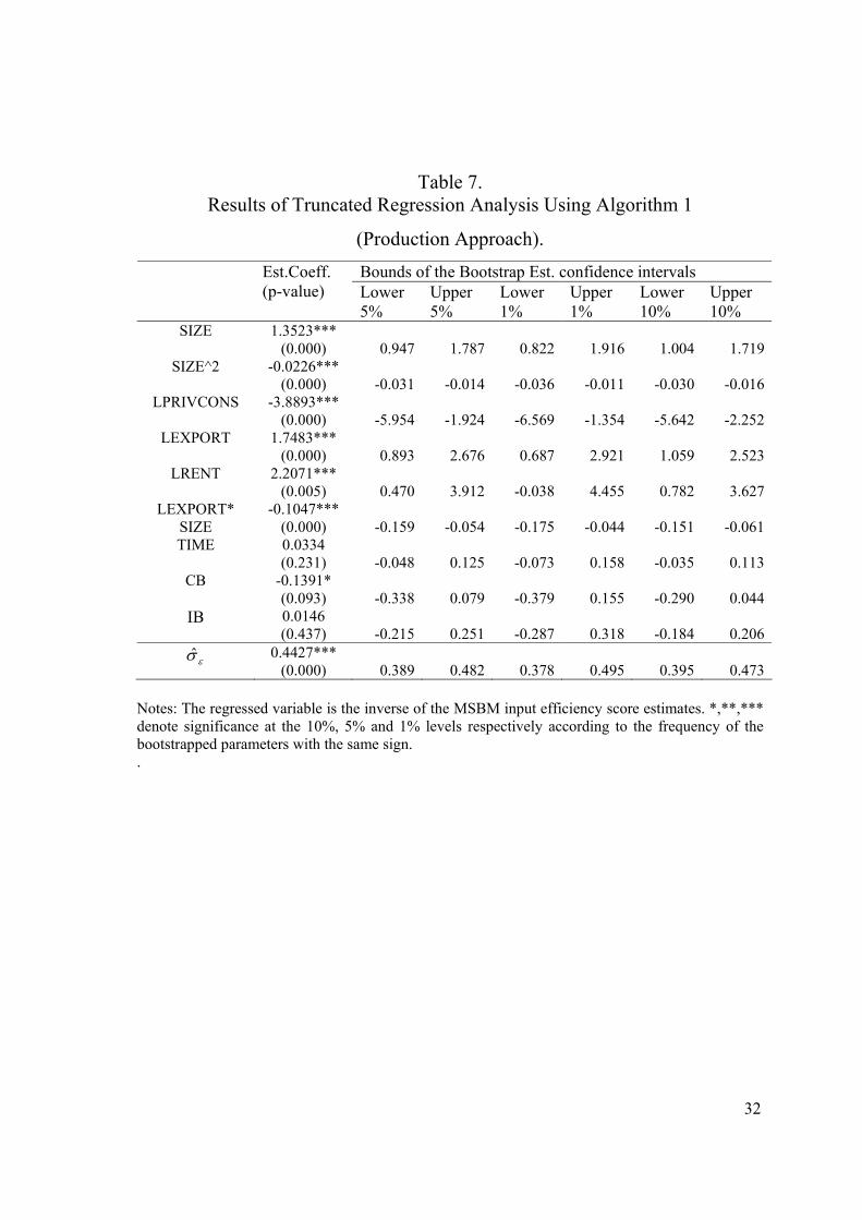
Tables 6 and 7 present results of the truncated regression analysis for the

Intermediation and Production approaches respectively. The following macroeconomic

variables were used in the specification of the truncated regression and gave the model with

the best fit: LPRIVCONS - log of private consumption; LEXPORT - log of net exports (sum of

the net export of services and the net export of goods); and LRENT - log of the rent for

private flats on Hong Kong Island (as a proxy for housing expenditure). To capture the

effects of time and bank specific characteristics, we further included a time trend (TIME)

variable along with group dummies. Additionally, to capture the effects of scale we included

the SIZE variable (log of total deposits) and the square of SIZE (SIZE^2). Finally, we

included the interaction variable of the LEXPORT and SIZE (LEXPORT_SIZE) to capture the

effect of the exportability of financial services of Hong Kong banks depending on the size of

banking firm. According to the Information Services Department of the Hong Kong Special

Administrative Region Government, in 2006, the share of exports of the financial services

industry was 12% of the total value of the export of services. Therefore, it is particularly

20

appealing to examine the influence of this variable on the efficiency of Hong Kong banking

firms.

INSERT TABLES 6 AND 7

It is interesting to note that, although the significance of the variables is different for

the inverse of the SBM efficiency scores under both Production and Intermediation

approaches, the signs of the explanatory variables are the same. In both models, the

indicators of size are found to be significant at the 1% level of significance with a positive

coefficient for SIZE and a negative one for SIZE^2. This implies that in the Hong Kong

banking industry, smaller banks are more efficient than their larger counterparts. However,

larger banks are more likely to enjoy gains from scale economies. This is thus empirical

evidence for the U-shaped scale economies implied by the theoretical literature. Moreover,

similar signs of coefficients were found by Simar and Wilson (2007) in their empirical

investigation of US commercial banks.

With respect to the macroeconomic determinants of banking (in)efficiency, the results

suggest that the level of private consumption has a negative impact on banking inefficiency

as expected. This implies that an increase in private consumption stimulates banking. Both

LRENT and LEXPORT are found to be positively correlated with inefficiency and significant

at the 1% level in the Production approach model and at the 10% level under the

Intermediation framework. Interestingly, the coefficient for the interaction variable

LEXPORT_SIZE is negative and significant in the Intermediation approach at the 10% level

and with respect to the Production methodology, at the 1% level. This suggests that larger

banks show a greater exportability of financial services. It can also be interpreted as larger

banks having more opportunities to engage in exporting activities, thereby enhancing their

efficiency.

Intriguingly, the results also show that the coefficient for the commercial banks’

dummy is negative and significant in both models, whereas the coefficient of IB is negative

and significant only in the Intermediation model.6 This implies that commercial banks are

6 The dummy for bank holdings and holding companies was dropped from the model due to collinearity problems.

21

successful under both intermediation and service-producing objectives, whereas investment

banks are only successful under the former..

5. Conclusions

The analysis presented in this paper shows that, under both the Intermediation and

Production approaches, Hong Kong banks suffered a substantial decline in efficiency in the

year 2001. This was probably due to deposit rate deregulation and the adverse consequences

of the 9/11 terrorist attacks in the US. Utilising a relatively-new technique (Sharp et al.

(2006)) to purge the Slacks-Based Methodology scores of any random error, we also find that

the efficiency of banks was most affected in 2001. Adoption of the latter model is necessary

because exogenous events can lead to ‘bad luck’ and hence interfere with the managerial

operations of banks. Indeed, in the analysis of subsequent years, it was found that the same

exogenous events which happened economy-wide could have a negative or positive effect on

the efficiency results dependent on the bank sector considered. For example, under the

Intermediation approach, commercial banks experienced negative bias and investment banks

positive bias during 2004-2006 (see Table 3). Finally, with respect to the bias-corrected

efficiency scores, commercial banks were consistently closer to the best practice frontier than

the other sectors of the industry (see Figures 1 and 2), starting at 0.937 (2000) and ending at

0.972 (2006) under the Intermediation approach.

Having obtained the bias-corrected efficiency scores, we proceeded to analyse the

effects of macroeconomic factors on bank efficiency. Utilising a ‘general-to-specific’ step-

down procedure we found that all but the time trend (the other variables being private

consumption, net exports and rent (all in logarithmic form)), had a significant effect on bank

efficiency scores over the sample period, under both the Intermediation and Production

approaches. It was interesting to find that the smaller banks were more efficient than the

larger banks, but the latter were also able to enjoy economies of scale. This size factor was

linked to the exportability of financial services, whereby the larger banks enjoyed a positive

effect on bank efficiency given their ability to export services.

22

Finally, it is worth re-iterating that we found that the commercial banks enjoyed

relative efficiency improvements over the sample period due to their ability to combine both

intermediary and service-producing business activities. A possible policy conclusion from

these results is that the financial system within Hong Kong could be further deregulated for

non-commercial banks, hence allowing a possible increase in stability of the financial

markets if a future Asian Financial Crisis, or any other ‘bad luck’ scenario in the World

economy, happened. Thus, deregulation could allow for further diversification for, as we

have seen, the banks which are able to diversify their assets most, appear to be the most

insulated against external shocks with respect to their efficiency.

23

References Akhigbe, A. and McNulty, J.E. (2003), “The Profit Efficiency of Small US Commercial

Banks,” Journal of Banking and Finance, 27, 307-325.

Altunbas, Y., Liu, M-H., Molyneux, P. and Seth, R. (2000), “Efficiency and Risk in Japanese

Banking,” Journal of Banking and Finance, 24, 1605-1628.

Banker, R.D., Charnes, A. and Cooper, W.W. (1984), “Some Models for the Estimation of

Technical and Scale Inefficiencies in Data Envelopment Analysis,” Management

Science, 30, 1078–1092.

Charnes, A., Cooper, W. and Rhodes, E. (1978), “Measuring the Efficiency of Decision-

Making Units,” European Journal of Operational Research, 2, 429 – 444.

Drake, L. and Hall, M. J. B. (2003), “Efficiency in Japanese Banking: An Empirical

Analysis,” Journal of Banking and Finance, 27, 891-917.

Drake, L., Hall, M.J.B. and Simper, R. (2006), “The Impact of Macroeconomic and

Regulatory Factors on Bank Efficiency: A Non-Parametric Analysis of Hong Kong’s

Banking System,” Journal of Banking and Finance, 30, 1443-1446.

Drake, L., Hall, M.J.B. and Simper, R. (2008), “Bank Modeling Methodologies: A

Comparative Non-Parametric Analysis of Efficiency in the Japanese Banking Sector,”

Journal of International Financial Markets, Institutions and Money, 18, forthcoming.

Färe, R. and Zelenyuk, V. (2003), “On Aggregate Farrell Efficiencies,” European Journal of

Operations Research, 146:3, 615-621.

Fare, R., Grosskopf, S. and Lovell, C.A.K. (1985), The Measurement of Efficiency of

Production. Kluwer- Nijhoff Publishing, Boston.

Farrell, M.J. (1957), “The Measurement of Productive Efficiency,” Journal of the Royal

Statistical Society, Ser. A, 120, 253-281.

Fried, H.O., Schmidt, S.S. and Yaisawarng, S. (1999), “Incorporating the Operating

Environment into a Nonparametric Measure of Technical Efficiency,” Journal of

Productivity Analysis, 12, 249-267.

Goldstein, M. (1998), The Asian Financial Crisis: Causes, Cures and Systemic Implications,

Institute for International Economics, Washington D.C., June.

24

Hall, M.J.B. (1985), “The Reform of Banking Supervision in Hong Kong,” Hong Kong

Economic Papers, No.16, pp.74-96, Hong Kong, August.

HKMA (2002), Annual Report, 2002, Hong Kong.

HKMA (2004), ‘Developments in the Banking Sector’, Quarterly Bulletin, March, 81-89.

Hunter, W.C., Kaufman, G.G. and Krueger, T.H. (eds.) (1999), The Asian Financial Crisis:

Origins, Implications and Solutions, Kluwer Academic Publishers

Jao, Y.C. (2001), The Asian Financial Crisis and the Ordeal of Hong Kong, Quorum Books,

Greenwood Publishing.

Jao, Y.C. (2003), ‘Financial Reform in Hong Kong,’ Chapter 6 in Hall, M.J.B. (ed.), The

International Handbook on Financial Reform, Edward Elgar Publishing, Cheltenham.

Krishnasamy, G., Ridzwa, A. H. and Perumal, V. (2003), “Malaysian Post Merger Banks’

Productivity: Application of Malmquist Productivity Index,” Managerial Finance, 30,

63-74.

Kwan, S. (2002), “The X-Efficiency of Commercial Banks in Hong Kong,” Hong Kong

Institute for Monetary Research, Working Paper No. 12/2002.

Laeven, L. and Majnoni, G. (2003), “Loan Loss Provisioning and Economic Slowdowns:

Too Much, Too Late?” Journal of Financial Intermediation, 12, 178-197.

Li, Q. (1996), “Nonparametric Testing of Closeness between Two Unknown Distributions”,

Econometric Reviews, 15, 261-274.

Lozano-Vivas, A., Pastor, J.A. and Pastor, J.M. (2002), “An Efficiency Comparison of

European Banking Systems Operating under Different Environmental Conditions,”

Journal of Productivity Analysis, 18, 59-77.

Pastor, J. T. (1996), “Translation Invariance in Data Envelopment Analysis: A

Generalization,” Annals of Operations Research, 66, 93–102.

Sealey, C. and Lindley, J.T. (1977), “Inputs, Outputs and a Theory of Production and Cost at

Depository Financial Institutions,” Journal of Finance, 32, 1251-1266.

Sharp, J.A., Meng, W. and Liu, W. (2006), “A Modified Slacks-Based Measure Model for

Data Envelopment Analysis with ‘Natural’ Negative Outputs and Inputs,” Journal of

the Operational Research Society, 1-6.

25

Sheather, S. J. and Jones, M.C. (1991), “A Reliable Data-Based Bandwidth Selection Method

for Kernel Density Estimation,” Journal of the Royal Statistical Society, Ser. B, 53(3),

683–690.

Shen, C-H. (2005), “Cost Efficiency and Banking Performance in a Partial Universal

Banking System: Application of the Panel Smooth Threshold Model,” Applied

Economics, 37, 993-1009.

Silva Portela, M.C.A, Thanassoulis, E. and Simpson, G. (2004), “Negative Data in DEA: A

Directional Distance Approach Applied to Bank Branches,” Journal of the

Operational Research Society, 55, 1111-1121.

Silverman, B. W. (1986), Density Estimation for Statistics and Data Analysis. Chapman and

Hall, London, UK.

Simar, L. and Wilson P.W. (2007), “Estimation and Inference in Two-Stage Semi-Parametric

Models of Production Processes,” Journal of Econometrics, 136, 31–64.

Simar, L. and Zelenyuk, V. (2006), “On Testing Equality of Two Distribution Functions of

Efficiency Scores Estimated from DEA,” Econometric Reviews, 25, 497-522.

Simar, L. and Zelenyuk, V.(2007), “Statistical Inference for Aggregates of Farrell-Type

Efficiencies,” Journal of Applied Econometrics, forthcoming.

Tone, K. (2001), “A Slack – Based Measure of Efficiency in Data Envelopment Analysis,”

European Journal of Operational Research, 130, 498 – 509.

Tortosa-Ausina, E. (2002), “Bank Cost Efficiency and Output Specification,” Journal of

Productivity Analysis, 18, 199-222.

Wand, M. P. and Jones, M.C. (1994), “Multivariate Plug-in Bandwidth Selection,”

Computational Statistics 9, 97–116.

World Bank. (1993), The East Asian Economic Miracle, Oxford University Press, New York.

26

Table 1

Liberalisation and Reform of the Hong Kong Banking Industry Post

1999: A Chronology of Major Events

Event Date

Interest rate cap on time deposits of less than 7 days was lifted, along with the prohibition on the provision of benefits to depositors (other than for Hong Kong dollar savings and current accounts)

3 July 2000

Deposit rate deregulation (of savings and current accounts) completed 3 July 2001

The "three-building" restriction imposed on foreign banks was removed

November 2001

Relaxation of market entry criteria for foreign banks May 2002

Government announced that, with effect from 1 January 2004, banks licensed in the territory will be allowed to accept deposits, arrange remittances, make foreign exchange transactions and issue credit and debt cards in renminbi. [Renminbi-denominated corporate banking operations remain off limits, however, for the time being.] This announcement followed the People’s Bank of China’s decision to provide clearing arrangements for Hong Kong’s licensed banks for personal renminbi business transacted in Hong Kong

November 2003

Deposit insurance introduced. 2006

Source: Jao, 2003.

27

Table 2. Hong Kong Banks: Summary Statistics

mean min max st. dev Total Operating Expenses 1541876 1800 45167256 4659830 Fixed Assets 2769599 100 49216374 7331098 Total Deposits and Funding 122029945 1761 3249308598 358086443Total Loans 61695841 338 1229425206 162984058Other Earning Assets 67505775 0 1993631331 205726006Loan loss provisions 318161 -3104460 8593000 1092042 Net com Income + Other operating Income 1174795 -1865023 38054181 4019743

All figures in HK$ millions and deflated using the Hong Kong GDP deflator.

28

Table 3. Group-Wise Heterogeneous Sub-Sampling Bootstrap Aggregate Efficiencies

Under the Intermediation Approach 2000 2001 2002 2003 2004 2005 2006BHHC – Bank Holdings and Holding Companies Original SBM score 0.827 0.659 0.714 0.747 0.874 0.743 0.905

Bias-corr SBM eff. 0.821 0.585 0.517 0.641 0.866 0.661 0.868Stn.dev. 0.092 0.115 0.094 0.069 0.103 0.049 0.109

CI 5% Up 0.669 0.360 0.428 0.521 0.748 0.560 0.811

Bootstrap estimates

CI 5% Lo 0.976 0.793 0.767 0.773 1.115 0.749 1.204

CB – Commercial Banks Original SBM score 0.893 0.712 0.756 0.873 0.922 0.931 0.935

Bias-corr SBM eff. 0.937 0.560 0.699 0.862 0.926 0.967 0.972Bootstrap

estimates Stn.dev. 0.068 0.065 0.116 0.073 0.087 0.061 0.074 CI 5% Up 0.822 0.455 0.538 0.768 0.880 0.884 0.889 CI 5% Lo 1.096 0.705 0.944 1.041 1.219 1.107 1.131IB – Investment Banks Original SBM score 0.745 0.681 0.623 0.662 0.792 0.687 0.669

Bias-corr SBM eff. 0.684 0.499 0.362 0.515 0.668 0.551 0.458Bootstrap

estimates Stn.dev. 0.075 0.042 0.055 0.047 0.036 0.048 0.062 CI 5% Up 0.573 0.426 0.285 0.426 0.612 0.469 0.346 CI 5% Lo 0.863 0.588 0.484 0.613 0.749 0.660 0.588All Banks Original SBM score 0.860 0.699 0.733 0.827 0.898 0.891 0.911Bootstrap estimates

Bias-corr SBM eff. 0.881 0.560 0.618 0.788 0.938 0.905 0.919

Stn.dev. 0.059 0.066 0.088 0.058 0.071 0.050 0.068 CI 5% Up 0.776 0.453 0.499 0.704 0.833 0.829 0.843 CI 5% Lo 1.003 0.707 0.828 0.917 1.105 1.019 1.091

Notes: We use 1000 group-wise heterogeneous bootstrap replications, Gaussian density, and the Silverman (1986) reflection method; and the bandwidth is obtained using the Sheather and Jones (1991) solve-the-equation plug-in-approach. CI 5% Up and CI 5% Lo indicate 5% Confidence Intervals at the Upper and Lower levels respectively.

29

Table 4. Group-Wise Heterogeneous Sub-Sampling Bootstrap Aggregate Efficiencies

Under the Production Approach 2000 2001 2002 2003 2004 2005 2006BHHC – Bank Holdings and Holding Companies Original SBM score 0.867 0.584 0.605 0.654 0.827 0.637 0.868

Bias-corr SBM eff. 0.962 0.545 0.359 0.600 0.836 0.530 0.756Stn.dev. 0.113 0.067 0.125 0.066 0.107 0.073 0.056

CI 5% Up 0.764 0.390 0.210 0.453 0.686 0.375 0.735

Bootstrap estimates

CI 5% Lo 1.160 0.658 0.673 0.692 1.065 0.620 0.893

CB – Commercial Banks Original SBM score 0.691 0.617 0.652 0.739 0.879 0.887 0.902

Bias-corr SBM eff. 0.632 0.424 0.656 0.612 0.985 0.916 0.938Bootstrap

estimates Stn.dev. 0.081 0.079 0.122 0.082 0.091 0.073 0.072 CI 5% Up 0.466 0.282 0.410 0.507 0.820 0.809 0.827 CI 5% Lo 0.795 0.569 0.863 0.810 1.172 1.080 1.098IB – Investment Banks Original SBM score 0.671 0.603 0.493 0.556 0.573 0.586 0.591

Bias-corr SBM eff. 0.615 0.432 0.238 0.365 0.254 0.377 0.369Bootstrap

estimates Stn.dev. 0.074 0.051 0.054 0.053 0.048 0.057 0.090 CI 5% Up 0.488 0.327 0.118 0.258 0.168 0.285 0.193 CI 5% Lo 0.780 0.531 0.341 0.474 0.356 0.494 0.526All Banks Original SBM score 0.708 0.609 0.619 0.697 0.820 0.825 0.866Bootstrap estimates

Bias-corr SBM eff. 0.666 0.452 0.521 0.586 0.837 0.815 0.851

Stn.dev. 0.069 0.066 0.100 0.068 0.072 0.060 0.062 CI 5% Up 0.536 0.322 0.353 0.472 0.707 0.717 0.755 CI 5% Lo 0.793 0.570 0.715 0.718 0.983 0.944 0.990

Notes: We use 1000 group-wise heterogeneous bootstrap replications, Gaussian density, and the Silverman (1986) reflection method; and the bandwidth is obtained using the Sheather and Jones (1991) solve-the-equation plug-in-approach. CI 5% Up and CI 5% Lo indicate 5% Confidence Intervals at the Upper and Lower levels respectively.

30

Table 5. Simar-Zelenyuk-Adapted Li Test for Equality of Efficiency Distributions

Null Hypothesis Test Statistics Bootstrap p-value

f(EffProd) = f(EffInterm) 15.681 0.000**

f(EffProdBHHC) = f(EffIntermBHHC) 1.6015 0.0396*

f(EffProdCB) = f(EffIntermCB) 5.4755 0.000**

f(EffProdIBSH) = f(EffIntermIBSH) 10.660 0.000**

Notes: (Interm) Intermediation Approach, (Prod) Production Approach. The number of bootstrap iterations is 5000. For these tests, we use the Gaussian density, and h is the minimum of the two bandwidths for EFFM1 and EFFM2, which are calculated according to Silverman (1986). Statistical significance: * statistically significant at 5% level; ** statistically significant at 1% level.

31

Table 6. Results of Truncated Regression Analysis Using Algorithm 1

(Intermediation Approach). Bounds of the Bootstrap Est. confidence intervals Est.Coeff.

(p-value) Lower 5%

Upper 5%

Lower 1%

Upper 1%

Lower 10%

Upper 10%

SIZE 1.6990*** (0.000) 0.812 2.717 0.656 3.210 0.922 2.482

SIZE^2 -0.0403*** (0.000) -0.064 -0.022 -0.077 -0.018 -0.059 -0.024

LPRIVCONS -4.4699** (0.012) -8.900 -0.396 -10.267 0.669 -8.036 -0.966

LEXPORT 1.3270* (0.073) -0.300 3.102 -1.093 3.681 -0.128 2.822

LRENT 3.0003* (0.059) -0.544 6.610 -1.780 8.141 -0.127 5.995

LEXPORT* SIZE

-0.0923* (0.052) -0.205 0.017 -0.268 0.058 -0.182 0.001

TIME 0.0697 (0.220) -0.115 0.255 -0.166 0.309 -0.082 0.220

CB -0.4404** (0.014) -0.781 -0.058 -0.896 0.107 -0.724 -0.128

IB -0.4528** (0.021) -0.855 -0.009 -0.935 0.151 -0.800 -0.083

εσ̂ 0.6234*** (0.000) 0.509 0.722 0.489 0.766 0.520 0.697

Notes: The regressed variable is the inverse of the MSBM input efficiency score estimates. *,**,*** denote significance at the 10%, 5% and 1% levels respectively according to the frequency of the bootstrapped parameters with the same sign.

32

Table 7. Results of Truncated Regression Analysis Using Algorithm 1

(Production Approach). Bounds of the Bootstrap Est. confidence intervals Est.Coeff.

(p-value) Lower 5%

Upper 5%

Lower 1%

Upper 1%

Lower 10%

Upper 10%

SIZE 1.3523*** (0.000) 0.947 1.787 0.822 1.916 1.004 1.719

SIZE^2 -0.0226*** (0.000) -0.031 -0.014 -0.036 -0.011 -0.030 -0.016

LPRIVCONS -3.8893*** (0.000) -5.954 -1.924 -6.569 -1.354 -5.642 -2.252

LEXPORT 1.7483*** (0.000) 0.893 2.676 0.687 2.921 1.059 2.523

LRENT 2.2071*** (0.005) 0.470 3.912 -0.038 4.455 0.782 3.627

LEXPORT* SIZE

-0.1047*** (0.000) -0.159 -0.054 -0.175 -0.044 -0.151 -0.061

TIME 0.0334 (0.231) -0.048 0.125 -0.073 0.158 -0.035 0.113

CB -0.1391* (0.093) -0.338 0.079 -0.379 0.155 -0.290 0.044

IB 0.0146 (0.437) -0.215 0.251 -0.287 0.318 -0.184 0.206

εσ̂ 0.4427*** (0.000) 0.389 0.482 0.378 0.495 0.395 0.473

Notes: The regressed variable is the inverse of the MSBM input efficiency score estimates. *,**,*** denote significance at the 10%, 5% and 1% levels respectively according to the frequency of the bootstrapped parameters with the same sign. .

33

Figure 1 Dynamics of Aggregate Efficiency of Banking Groups (Intermediation Approach)

0

0.1

0.2

0.3

0.4

0.5

0.6

0.7

0.8

0.9

1

2000 2001 2002 2003 2004 2005 2006

BHHCCB IBAll

Figure 2 Dynamics of Aggregate Efficiency of Banking Groups (Production Approach)

0

0.1

0.2

0.3

0.4

0.5

0.6

0.7

0.8

0.9

1

2000 2001 2002 2003 2004 2005 2006

BHHCCB IBAll

34

Figure 3. Distribution of SBM Efficiency Scores by Type of Banking Firm Under the Two Alternative

Approaches.

0 0.5 1 1.5 2 2.5 3 3.5 4 4.5 50

0.2

0.4

0.6

0.8

1

1.2

1.4Kernel Est. Densities of Indiv. Efficiency Scores (All banks)

IntermediationProduction

0 0.5 1 1.5 2 2.5 3 3.5 4 4.5 50

0.1

0.2

0.3

0.4

0.5

0.6

0.7

0.8

0.9

1Kernel Est. Densities of Indiv. Efficiency Scores (IBSH)

IntermediationProduction

0 0.5 1 1.5 2 2.5 3 3.5 4 4.5 50

0.2

0.4

0.6

0.8

1

1.2

1.4

1.6Kernel Est. Densities of Indiv. Efficiency Scores (CB)

IntermediationProduction

0 0.5 1 1.5 2 2.5 3 3.5 4 4.5 50

0.2

0.4

0.6

0.8

1

1.2

1.4Kernel Est. Densities of Indiv. Efficiency Scores (BHHC)

IntermediationProduction

Note. Vertical axis refers to (estimated) probability density function of the distribution of efficiency scores and horizontal axis refers to efficiency scores (reflected). The univariate Gaussian kernel is used, and the bandwidth is obtained using the Sheather and Jones (1991) solve-the-equation plug-in approach.

35

Figure 4. Normalised slacks-based efficiency iρ̂ ’s: transition across alternative output definitions.

Contour Plot of Norm.Indiv.Eff.Scores 2000-06

Intermediation

Pro

duct

ion

0.4 0.6 0.8 1 1.2 1.4 1.6 1.8 20.4

0.6

0.8

1

1.2

1.4

1.6

1.8

2

Note. The bivariate Gaussian kernel is used, and the bandwidths are calculated according to the solve-the-equation plug-in approach for the bivariate Gaussian kernel, based on Wand and Jones (1994).