1

Ensemble-based observation impact estimates

using the NCEP GFS

Yoichiro Ota1

National Centers for Environmental Prediction/Environmental Modeling

Center NCEP/NWS/NOAA, College Park, Maryland

John C. Derber

National Centers for Environmental Prediction/Environmental Modeling

Center NCEP/NWS/NOAA, College Park, Maryland

Eugenia Kalnay

University of Maryland, College Park, Maryland

Takemasa Miyoshi

University of Maryland, College Park, Maryland

RIKEN Advanced Institute for Computational Science, Kobe, Japan

1 Corresponding author address: Yoichiro Ota, National Centers for Environmental

Prediction/Environmental Modeling Center, 5830 University Research Court, College Park, MD 20740.

E-mail: yoichiro.ota@noaa.gov

2

Abstract

The impacts of the assimilated observations on the 24 hour forecasts are estimated with

the ensemble-based method proposed by Kalnay et al. using the ensemble Kalman filter

(EnKF). This method estimates the relative impact of observations in data assimilation

similarly to the adjoint-based method proposed by Langland and Baker but without using

the adjoint model. It is implemented with the National Centers for Environmental

Prediction (NCEP) Global Forecasting System (GFS) EnKF which has been used as a

part of operational global data assimilation system at NCEP since May 2012. The result

quantifies the overall positive impacts of the assimilated observations and the relative

importance of the satellite radiance observations compared to other types of observations

especially for the moisture variables. The method is also used to identify the cause of

local forecast failure cases in the 24 hr forecasts. Data denial experiments of the

observations identified as producing a negative impact observation sets reduce the

forecast errors as estimated, validating the impact estimate.

3

1. Introduction

Estimating the observation impacts within the numerical weather prediction (NWP)

system is an important step to improve the performance of the operational NWP. There

have been substantial efforts to estimate the impact of the assimilated observations by

carrying out data-denial experiments or the Observing System Experiments (OSE, e.g.

Bouttier and Kelly 2001, Zapotocny et al. 2007, 2008). OSEs provide the nonlinear

impacts on the accuracy of the forecasts with and without a certain set of observations.

However, carrying out OSEs with various observation datasets is computationally very

expensive. As an alternative, Langland and Baker (2004) proposed an approach to

estimate the observation impacts on the forecasts without performing OSEs using the

adjoint sensitivity analysis. This forecast sensitivity to observations approach can be

performed with relatively low computational cost and provides the impact of each

assimilated observations in a linear sense. It has been applied to several operational data

assimilation systems and has been proven to be effective in estimating the observation

impacts on the short-range forecasts and the performance of the data assimilation system

(Zhu and Gelaro 2008, Cardinali 2009). However, it requires the adjoint operators of the

forecast model and the data assimilation system. Liu and Kalnay (2008) and Li et al.

(2010) proposed a similar method using the ensemble Kalman filter (EnKF) without the

adjoint model. The ensemble-based approach is convenient for estimating the observation

impacts in the ensemble-based data assimilation system since it uses the ensemble

perturbations instead of the adjoint operators. Kunii et al. (2012) successfully applied the

ensemble-based approach to estimate the impact of real observations with the Weather

Research and Forecasting model using the Local Ensemble Transform Kalman Filter

4

(LETKF, Hunt et al. 2007) and estimated the impact of various observations on the

Typhoon forecast. Kalnay et al. (2012) proposed an improved formulation of the Liu and

Kalnay (2008) algorithm. It is simpler, more accurate (or makes fewer approximations),

and can be applied on other EnKF and not just the LETKF.

In this study, observation impact estimates within the EnKF have been

investigated. The formulation of Kalnay et al. (2012) was applied to the near operational

global data assimilation settings using real observations. In this study it was applied to

the NCEP Global Forecasting System EnKF (GFS/EnKF, Whitaker et al. 2008) with the

observations assimilated in the NCEP operational global data assimilation system. The

result provides the relative impacts of each observation type in the operational NWP

context. We show that it can also be used as an effective tool to investigate the origin of

local forecast failure cases that sometimes degrade the operational forecasts substantially.

Section 2 introduces the formulation of the ensemble-based approach used in this study.

Following section 3 with the experimental settings, section 4 presents the overall results

and section 5 focuses on the evaluation of the origin of local forecast failures. Finally,

section 6 provides a summary and discussion.

2. Ensemble-based formulation

We will estimate the forecast error reduction due to the assimilation of each observation.

The forecasts from the analysis ( f

tx ) and from the first guess ( xt

g ) are verified against the

analysis or any other values close to the truth ( x t

truth ) at forecast time t. We define the

forecast errors as,

truth

t

g

t

g

t

truth

t

f

t

f

t xxexxe −≡−≡ , . (1)

5

The overbars represent the ensemble mean and can be disregarded for the deterministic

analysis and forecast. Following Langland and Baker (2004), forecast error reduction is

defined as

( ) ( )g

t

f

t

g

t

f

t

g

t

g

t

f

t

f

t

gf

t CCCe eeeeeeeeTTT +−=−≡∆ −

2

1

2

1

2

1, (2)

where C is the norm operator, defining the measure of the forecast error. The forecast

error difference can be described as

( ) o

gag

t

f

t

g

t

f

t yMKxxMxxee δ=−≈−=− 00 , (3)

where x0

a and x0

g are the analysis and the first guess at time 0. M and K represent

tangent linear forecast model and Kalman gain matrix. Here, ( )g

oo H 0xyy −≡δ , where

oy and H are the observation vector and nonlinear observation operator, is known as the

vector of innovations. The forecast time t is assumed to be short, so that we can apply the

tangent linear model. From (2) and (3), the forecast error reduction from the assimilation

of observations is expressed as

[ ] ( ) ( )g

t

f

to

g

t

f

to

gf

t CCe eeMKyeeyMK TTTT+=+≈∆ − δδ

2

1

2

1. (4)

This equation is used for the observation impact estimates based on the adjoint

sensitivity. On the other hand, Kalman gain in the EnKF is

1

001

1 −

−= RHXXK TTaa

K, (5)

where K, X0

a , and R are the ensemble size, the matrix of analysis perturbations and the

observation error covariance, respectively. (4) can also be described as

6

( )

( )[ ] ( )

( )( ) ( )g

t

f

t

f

t

a

o

g

t

f

to

aagf

t

CK

CK

e

eeXHXRy

eeyRHXMX

TT

TT

+−

≈

+−

≈∆

−

−−

0

1

1

00

12

1

12

1

δ

δ

. (6)

This equation is used for this study to estimate observation impacts. It is simpler and

computationally more efficient than the original formulation of Liu and Kalnay (2008)

and Li et al. (2010) and also can be easily applied to deterministic EnKFs other than the

LETKF (Kalnay et al. 2012).

As the EnKF requires covariance localization when the number of degrees of

freedom is much larger than the number of the ensemble members, the ensemble-based

observation impact estimates also require localization in practical applications. Following

Kalnay et al. (2012), we achieve this by computing the impact of l th observation on

forecast at j th grid point as

( )( )

( ) ( )( ) ( )[ ]lj

g

t

f

tjjj

f

t

a

jlolj

gf

t CK

e eeXHXRy T +−

=∆ −−0

1

,12

1ρδ , (7)

where ρ j is the localization function at grid point j for the l th observation. The

localization function in (7) may be different from the one used in the EnKF analysis

especially when the impact of the observations on the forecast moves during the forecast

away from the initial location.

3. Experimental settings

Equation (7) is applied to the NCEP GFS/EnKF analysis and forecast ensembles. The

horizontal resolution of the GFS in this experiment is T254 (about 55 km) and it has 64

sigma-p hybrid vertical layers up to 0.3 hPa. The serial Ensemble Square Root Filter

(EnSRF, Whitaker and Hamill 2002) is applied for the EnKF analysis. EnKF employs 80

7

members and assimilates observations every 6 hours. The use of the ensembles allows

one to measure the forecast error with both dry and moist total energy norm (Ehrendorfer

et al. 1999) in the global domain and the verifications are made against its own analysis.

( ) dSdqTC

Lwp

P

TRT

T

Cvu

STE

S rp

qs

r

rd

r

p σ∫ ∫

′+′+′+′+′=1

0

22

2

2

2221

2

1. (8)

Here ′u , ′v , ′T , ′ps and ′q are the forecast errors of zonal wind, meridional wind,

temperature, surface pressure and specific humidity, respectively. Cp, Rd and L are the

specific heat at constant pressure, gas constant of dry air and latent heat of condensation

per unit mass, respectively. Tr and Pr are reference temperature and pressure, respectively

(we used 280 K and 105 Pa). wq is 1 for moist total energy and 0 for dry total energy.

Evaluation forecast time is chosen to be 24 hours.

The fifth order polynomial of Gaspari and Cohn (1999) is used as the covariance

localization function with a cutoff length (where localization function becomes 0) at 2.0

scale heights for the vertical and 2000 km for the horizontal (corresponding to about 0.8

scale heights and 800 km with e-folding scales).

The localization scale for observation impact estimate is chosen to be the same as

the EnKF analysis update. Since observation impacts evolve through the forecast, the

localization function also needs to evolve. We tested both a fixed localization function as

in the EnKF analysis and a mobile localization function with the center position moving

with 0.75 times the average of analysis and forecast horizontal wind at each vertical level.

Multiplicative inflation (Anderson, 2001) proportional to the spread reduction by analysis

update is applied so that the amount of spread reduction becomes 15 % of the original

8

reduction. Also additive inflation using 0.32 times of randomly selected 24 and 48 hour

forecast lagged differences is applied. These are the same settings as the EnKF analysis

part of the NCEP operational global system. The assimilation cycles are performed from

00 UTC, January 1, 2012 to 18 UTC, February 8, 2012. The first week is discarded as

operational assimilation system is still in spin-up mode and the last 1 month (from

January 8 to February 7, 4 cycles per day, 124 cases) is used for the observation impact

estimates. Forecast errors are verified against their own analysis. All observation types

used in the NCEP operational global analysis (operational since May 2012, about 3.3

million observations in each analysis) except for satellite-based precipitation rate

retrievals from TRMM/TMI are assimilated. Table 1 shows the observation types

assimilated in this experiment. The same satellite radiance bias correction coefficients as

the hybrid EnKF / 3DVAR experiment (the operational global data assimilation system

since May 2012) are applied.

4. Results

a. The effect of a moving localization

First, the effect of localization on the observation impact estimates is examined. Figure 1

shows the time series of the total forecast error reduction. The actual forecast error

reduction is verified against its own analysis. If the impact estimate was perfect, it would

be identical with the actual error reduction. The error reduction is generally larger at 00

and 12 UTC than at 06 and 18 UTC because more conventional observations are

available at 00 and 12 UTC. Observation impact estimates with the moving localization

capture better the diurnal cycles than that with the fixed localization. Correlations of total

9

impact estimates to the true forecast error reduction are 0.318 with the fixed localization

and 0.730 with the moving localization. The average impact estimation is larger for the

moving localization. As suggested by Kalnay et al. (2012), special attention is required

on the localization on the ensemble-based observation impact estimates. Although our

approach is very simple and may not be optimal, the moving localization applied in this

experiment works well in our real data assimilation problem. In the following sections,

only the results with the moving localization are shown.

b. Estimated impacts of each observation type

Figure 2a shows the average 24 hour forecast error reduction estimates with the moist

total energy contributed from each observation type during the experiment. Negative

values correspond to the reduction of the forecast error due to the assimilation of the

observations. All observation types except Ozone retrievals are estimated to reduce the

forecast error on average in this period. In the EnKF, ozone observations are assimilated

with a univariate covariance, i.e., only the ozone analysis is changed, with no impact on

other variables at the analysis time, thus limiting the impact of the ozone observations on

the forecast. For the overall impacts, AMSUA shows the largest contribution to the

forecast error reduction. IASI and Aircraft are the second and the third, followed by

radiosondes and AIRS.

The observation impact per observation is obtained by dividing the total impact

by the observation count (Figure 2b). TCVital observations of tropical cyclones have

extremely large impact per observation but the sample number is small (79 observations

during the entire period and only in the Southern Hemisphere). Dropsonde observations

also have very large impacts on average. Most of the dropsondes were deployed over the

10

Northeastern Pacific during the Winter Storm Reconnaissance program (Toth et al. 2002)

led by National Oceanic and Atmospheric Administration (NOAA). This program aims to

reduce the short-range forecast error of the strong extratropical cyclones using the

observation targeting strategy (Bishop et al. 2001, Majumdar et al. 2002). The result

suggests that this program is effective in reducing the forecast error. Other than these,

conventional upper-air observations such as PIBAL and Radiosonde have large impacts

per observation. Satellite scatterometer winds (ASCAT_Wind and WINDSAT_Wind)

and marine surface observations also have relatively large impacts. Total contributions of

those observations to the forecast error reduction are not so large, but those observations

are more effective per observation.

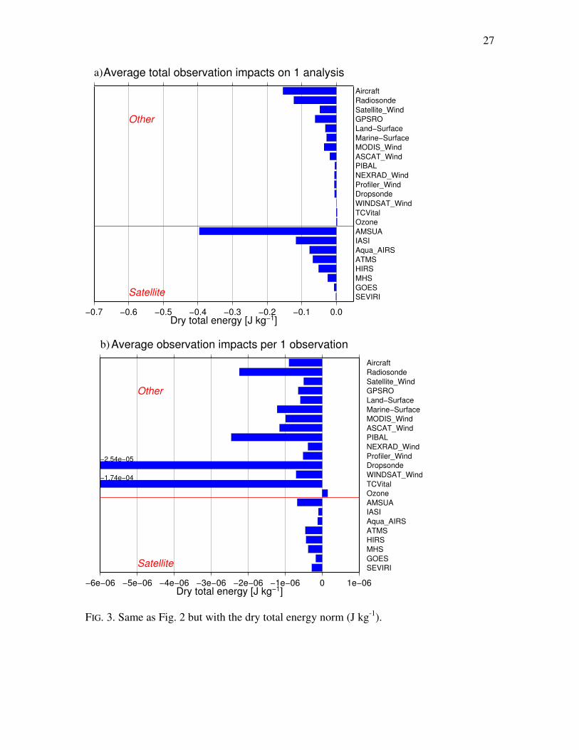
Figure 3 is a similar plot as figure 2 but measured using the dry total energy.

Comparing with figure 2, the impacts of the most satellite radiance observations are

substantially reduced, especially for the MHS. PIBALs’ impact per observation is also

reduced. Those observations are estimated to have impacts mostly on the forecast of

moisture variable. This is consistent with the facts that MHS is sensitive to the

atmospheric moisture, and most pilot balloons are used in the India, Southeast Asia and

Australia (summer in this period) where the atmospheric moisture is high. On the other

hand, some observations such as GPSRO and MODIS wind have similar impacts with the

moist and dry total energy indicating that they did not impact the moisture forecast. Most

of the assimilated GPSRO observations measure the atmosphere above the upper

troposphere, so that their impacts are large in the upper layer where the atmosphere is

dry. MODIS wind covers the Arctic and Antarctic regions where the atmospheric

moisture is scarce especially during the winter. The fractional impact of the satellite

11

radiances is 65% for the moist total energy and 59% for the dry total energy. This

suggests that the impact of satellite radiance observations is important especially in the

forecast metric related to moisture.

c. Estimated impacts of each observation element

Figure 4 represents the AIRS satellite radiance impact estimates classified by each

channel. Most of the channels have positive impact on the forecast. Some channels are

estimated to have relatively large impacts and others show small impacts and even show

small negative impacts for several channels. This information may help guide the better

use of the satellite radiances. Figure 4 also shows the estimates using the dry total energy

norm. Note that the impact estimates are substantially different from the one with moist

total energy. The impacts are dependent on the selection of the error metric. Therefore,

one should be careful to choose an appropriate error norm to estimate the observation

impacts. Compared to the result with the moist total energy, the large peaks around

channel 215 to 1627 have been reduced. This suggests that these channels are sensitive to

moisture forecast.

Figure 5 shows the impact of a) RAOB and b) aircraft per observation classified

by the observation level. For the radiosonde observations, observations on the lower and

middle troposphere have the largest impact on the forecast. On the other hand, aircraft

observations on the lower troposphere have smaller impacts compared to the radiosonde

observations. Figure 6 compares the average number of the assimilated radiosonde and

aircraft observations per analysis time. Horizontal distributions of the radiosonde

observations are almost the same as at 600 – 800 hPa and at 125 – 250 hPa. For the

aircraft observations, the distributions are completely different. Observations at 125 –

12

250 hPa are spread widely along the major flight tracks over data-sparse regions.

However, aircraft observations in the lower troposphere are only distributed around the

airports and are much denser than the radiosonde observations. This geographical

distribution of the aircraft observations in the lower troposphere and near airports that

often have other conventional observations seems to limit their impacts on NWP.

Observation impact estimates also provide the geographical distribution of the

impact and relative importance of the observations. Figure 7 shows the average impacts

of radiosonde per profile from fixed land stations in this experimental period. Overall,

observations from most of the stations have positive impacts. Relatively large impacts are

seen in the Tropics and also in Canada, Australia and South America.

Figure 8 shows the comparison of the radiosonde observations from two

neighboring stations (Narssassuaq and Egedesminde in Greenland). Compared to the

observations from Egedesminde, observations from Narssassuaq have large negative

impact especially for temperature and wind observations on troposphere. Figure 8b and

8c show the statistics of observation minus the first guess of temperature and wind speed.

Both statistics show the larger standard deviation for Narssassuaq. It does not

automatically determine that the observations from this station have poor quality, but

these observations do seem to have a detrimental impact on the short-range GFS forecast.

5. Estimation and attribution of short-range regional forecast

failures

The operational NWP forecasts sometimes fail despite their relatively high average

performance over the short-range forecasts. For the operational NWP centers, it is critical

13

to minimize the occurrence of such bad forecasts, and if possible take corrective

measures. Observation impact estimates may help finding a possible cause of large short-

range forecast errors in some of the cases.

In order to explore this potential use, local 24 and 30 hour forecast errors with the

moist total energy norm were computed over regions of 30o by 30

o areas covering the

whole globe with 10o increments for both latitude and longitude. For this purpose, cases

of local forecast failure were identified as failures if the following conditions were

satisfied: 1) The 24 hour forecast error was larger than twice its time average, and 2) The

24 hour forecast error was larger than 1.2 times of the error of 30 hour forecast from the

previous analysis. Table 2 shows the list of the identified cases. If the neighboring areas

on the same initial time also meet the criteria, they are considered to be the same case and

only the area with the highest error times error increase is shown in the table (the number

of identified areas is also shown). With these criteria, we identified 7 cases of local short-

range forecast failures in this period.

Observation impacts are estimated targeting these local forecast failures. The top

1 or 2 observation types estimated to have large negative impacts are removed from the

observation datasets. These “denied” observations are selected locally based on their

impact distribution so that the denial does not create a large difference on other areas.

Then, the analysis and the 24 hour forecast are reprocessed with the new observation sets.

Table 2 also shows the denied observations and change of the 24 hour forecast error in

the data denial experiment. The local forecast errors are in fact reduced in all 7 cases by

the observation denial.

14

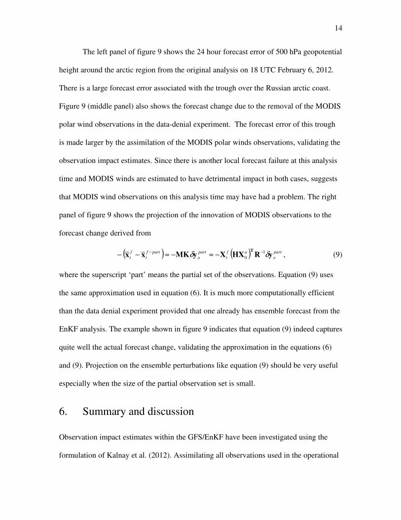
The left panel of figure 9 shows the 24 hour forecast error of 500 hPa geopotential

height around the arctic region from the original analysis on 18 UTC February 6, 2012.

There is a large forecast error associated with the trough over the Russian arctic coast.

Figure 9 (middle panel) also shows the forecast change due to the removal of the MODIS

polar wind observations in the data-denial experiment. The forecast error of this trough

is made larger by the assimilation of the MODIS polar winds observations, validating the

observation impact estimates. Since there is another local forecast failure at this analysis

time and MODIS winds are estimated to have detrimental impact in both cases, suggests

that MODIS wind observations on this analysis time may have had a problem. The right

panel of figure 9 shows the projection of the innovation of MODIS observations to the

forecast change derived from

( ) ( ) part

o

af

t

part

o

partf

t

f

t yRHXXyMKxxT

δδ 1

0

−− −≈−≈−− , (9)

where the superscript ‘part’ means the partial set of the observations. Equation (9) uses

the same approximation used in equation (6). It is much more computationally efficient

than the data denial experiment provided that one already has ensemble forecast from the

EnKF analysis. The example shown in figure 9 indicates that equation (9) indeed captures

quite well the actual forecast change, validating the approximation in the equations (6)

and (9). Projection on the ensemble perturbations like equation (9) should be very useful

especially when the size of the partial observation set is small.

6. Summary and discussion

Observation impact estimates within the GFS/EnKF have been investigated using the

formulation of Kalnay et al. (2012). Assimilating all observations used in the operational

15

global analysis (except for TRMM/TMI precipitation retrievals), the observation impacts

are estimated for each observation type. Satellite radiance observations are estimated to

be most important in reducing the short-range forecast error especially for moisture.

However, other observations such as aircraft observations, radiosonde, marine surface

observations and scatterometer winds are also very important. The last two observation

types have large impacts especially when the impacts per observation are measured.

Classified with the observation types and conditions, some examples of the

advantages and disadvantages of each observing system are shown. Aircraft observations

in the lower troposphere have smaller impacts per observation than the radiosondes

probably because of their geographical distribution. Estimated impacts of AIRS channels

show large positive impacts on the moisture and dynamical variables for many channels,

and small negative impacts for a few moisture channels, possibly indicating that the

radiances are not optimally assimilated. This information may guide the improvement of

the use of observations in the data assimilation and possibly the design of the observation

network. Continuous monitoring like Naval Research Laboratory (NRL) and National

Aeronautics and Space Administration / Global Modeling and Assimilation Office

(NASA/GMAO) do with the adjoint-based impact estimates may be beneficial in the

operational NWP system to detect the assimilated observations with poor quality.

We developed simple criteria to detect cases of “short range regional forecast

failures”, indicating that the 24 hr forecast be significantly worse than average, and worse

than the 30 hour forecast started 6 hr earlier. An analysis of cases of local short-range

forecast failure indicates that these observation impact estimates can be used as a tool to

identify those observations that may have caused the large forecast errors. The projection

16

of the observational innovation on the forecast change agrees well with the corresponding

data denial experiment, validating the approximation made on the formulation of the

observation impact estimates. We note that identifying short-range (12 or 24 hr) forecast

failures would make possible a more proactive QC approach where poor observations are

withdrawn and the analysis recomputed in time to improve longer forecasts. Such early

identification of flawed observations may guide studies to improve the algorithms with

which they are generated.

Although the application of this method is limited to ensemble based data

assimilation systems, there are many possible applications as several of the operational

NWP systems are transitioning to hybrid ensemble and variational data assimilation

system. One possible application is to use this method as an QC scheme as described

above. Ensemble perturbations from the hybrid analysis and forecasts may also be used

as inputs of the observation impact estimates. Further investigation in this promising area

is warranted.

Acknowledgments.

The authors thank Daryl Kleist (NCEP/EMC) for valuable discussion and his continuous encouragement of this work, and Dr. Mitch Goldberg for his support of this research. The EnKF data assimilation system used in this study was first developed by Jeff Whitaker (NOAA/ESRL). We appreciate Ricardo Todling (NASA/GMAO) for discussions and suggestions that helped us to understand better this method. This work was partially supported by a NESDIS/JPSS JPSS Proving Ground (PG) and Risk Reduction (RR) CICS Grant.

17

References

Ancell, A. and Hakim, G. J. 2007. Comparing adjoint- and ensemble-sensitivity analysis

with applications to observation targeting. Mon. Wea. Rev., 135, 4117-4134.

Anderson, J. L. 2001. An ensemble adjustment Kalman filter for data assimilation. Mon.

Wea. Rev., 129, 2884-2903.

Bishop, C. H., Etherton, B. J. and Majumdar, S. J. 2001. Adaptive sampling with the

ensemble transform Kalman filter. Part I: Theoretical aspects. Mon. Wea. Rev., 129, 420-

436.

Bouttier, F. and Kelly, G. 2001. Observing-system experiments in the ECMWF 4D-Var

data assimilation system. Quart. J. Roy. Meteor. Soc., 127, 1469-1488.

Cardinali, C. 2009. Monitoring the observation impact on the short-range forecast. Quart.

J. Roy. Meteor. Soc., 135, 239-250.

Ehrendorfer, M., Errico, R. M. and Raeder, K. D. 1999. Singular-vector perturbation

growth in a primitive equation model with moist physics. J. Atmos. Sci., 56, 1627-1648.

Gaspari, G. and Cohn, S. E. 1999. Construction of correlation functions in two and three

dimensions. Quart. J. Roy. Meteor. Soc., 125, 723-757.

18

Hunt, B. R., Kostelich, E. J. and Szunyogh, I. 2007. Efficient Data Assimilation for

Spatiotemporal Chaos: a Local Ensemble Transform Kalman Filter. Physica D, 230, 112-

126.

Kalnay, E., Ota, Y., Miyoshi, T. and Liu, J. 2012. A simpler formulation of forecast

sensitivity to observations: application to ensemble Kalman filters. Tellus, 64A, 18462,

http://dx.doi.org/10.3402/tellusa.v64i0.18462.

Kunii, M., Miyoshi, T. and Kalnay, E. 2012. Estimating impact of real observations in

regional numerical weather prediction using an ensemble Kalman filter. Mon. Wea. Rev.,

140, 1975-1987.

Langland, R. H. and Baker, N. L. 2004. Estimation of observation impact using the NRL

atmospheric variational data assimilation adjoint system. Tellus, 56A, 189-201.

Li, H., Liu, J. and Kalnay, E. 2010. Correction of 'Estimating observation impact without

adjoint model in an ensemble Kalman filter'. Quart. J. Roy. Meteor. Soc., 136, 1652-

1654.

Liu, J. and Kalnay, E. 2008. Estimating observation impact without adjoint model in an

ensemble Kalman filter. Quart. J. Roy. Meteor. Soc., 134, 1327-1335.

19

Majumdar, S. J., Bishop, C. H., Etherton, B. J. and Toth, Z. 2002. Adaptive sampling

with the ensemble transform Kalman filter. Part II: Field program implementation. Mon.

Wea. Rev., 130, 1356-1369.

Toth, Z., Szunyogh, I., Bishop, C., Majumdar, S., Morss, R., Moskaitis, J., Reynolds, D.,

Weinbrenner, D., Michaud, D., Surgi, N., Ralph, M., Parrish, J., Talbot, J., Pavone, J. and

Lord, S. 2002. Adaptive observations at NCEP: Past, present, and future. In Proceedings

of the symposium on observations, data assimilation, and probabilistic prediction, 13-17

January 2002, Orlando, Florida. American Meteorological Society, Boston, USA.

Whitaker, J. S. and Hamill, T. M. 2002. Ensemble data assimilation without perturbed

observations. Mon. Wea. Rev., 130, 1913-1924.

Whitaker, J. S., Hamill, T. M., Wei, X., Song, Y. and Toth, Z. 2008. Ensemble data

assimilation with the NCEP global forecast system. Mon. Wea. Rev., 136, 463-482.

Zapotocny, T. H., Jung, J. A., Marshall, J. F. L. and Treadon, R. E. 2007. A two-season

impact study of satellite and in situ data in the NCEP Global Data Assimilation System.

Wea. Forecasting, 22, 887-909.

Zapotocny, T. H., Jung, J. A., Marshall, J. F. L. and Treadon, R. E. 2008. A two-season

impact study of four satellite data types and rawinsonde data in the NCEP Global Data

Assimilation System. Wea. Forecasting, 23, 80-100.

20

Zhu, Y. and Gelaro, R. 2008. Observation sensitivity calculations using the adjoint of the

Gridpoint Statistical Interpolation (GSI) analysis system. Mon. Wea. Rev., 136, 335-351.

21

List of Figures

FIG. 1. Time series of the total forecast error reduction of each estimate (unit: J kg-1

).

Black, red, and blue lines show the actual forecast error reduction verified against the

own analysis, estimated error reduction from the EnKF-based method with fixed

localization (Fixed), and with moving localization (Advected). Numbers on upper left

corner show the correlation of each estimate to the actual forecast error reduction.

FIG. 2. Estimated average 24 hour forecast error reduction contributed from each

observation types (moist total energy, J kg-1

). a) represents the total error reduction and b)

represents error reduction per 1 observation.

FIG. 3. Same as Fig. 2 but with the dry total energy norm (J kg-1

).

FIG. 4. Estimated AIRS satellite radiance observation impacts classified by each channels

with the dry total energy (red, J kg-1

), and the moist total energy (blue, J kg-1

). Estimated

forecast error reduction by 1 observation is shown. Vertical bars represent the 95 %

confidence interval of the average values.

FIG. 5. Estimated average observation impacts of a) radiosonde and b) aircraft classified

by observed level (moist total energy, J kg-1

). Estimated forecast error reduction by 1

observation is shown.

22

FIG. 6. Average number of assimilated radiosonde observations a) from 250 to 125 hPa,

b) from 800 to 600 hPa and aircraft observations c) from 250 to 125 hPa and d) from 800

to 600 hPa in each 5o by 5

o area on 1 analysis.

FIG. 7. Average impact (moist total energy, J kg-1

) of 1 radiosonde profile from the fixed

land stations. Only the stations that have more than 20 profiles in the period are shown.

Numbers 4220 (Egedesminde) and 4270 (Narssassuaq) indicate the location of the

stations shown in Fig. 8 and 9.

FIG. 8. Comparison of the radiosonde observations from Narssassuaq (red line, 4270) and

Egedesminde (blue line, 4220) showing a) average impacts (J kg-1

) of each observation

element (solid: temperature, dashed: winds, dotted: humidity) on each pressure level by 1

profile and observation departure statistics (dashed: bias, solid: standard deviation) of b)

temperature (K) and c) wind speed (m s-1

).

FIG. 9. 24 hour forecast error of 500 hPa geopotential height (unit: m, 18 UTC February

6, 2012 initial) from original analysis (left) and forecast change due to the removal of the

observations (MODIS polar wind in 60N~90N, 30E~90E) in the data denial experiment

(middle: actual change and right: projection on the ensemble perturbations). Black

contours show the analysis. Magenta cones show the target area of the observation impact

estimate.

23

TABLE 1. Observation types assimilated in the experiment. The third column shows the

average number of observations assimilated on 1 analysis (in thousands). u, v, T, q and Ps

represents u and v wind components, temperature, specific humidity and surface pressure,

respectively.

Type of data Description Number

(thousands)

Aircraft u, v, and T observations from the aircrafts 173

Radiosonde Radiosonde observations (u, v, T, q and Ps) 55

Satellite_Wind Atmospheric Motion Vectors (u and v) from

geostationary satellites 96

GPSRO GPS radio occultation 95

Land-Surface Ps observations from land surface stations 54

Marine-Surface Surface u, v, T, q and Ps observations from the buoys

and ships 23

MODIS_Wind Atmospheric Motion Vectors (u and v) from MODIS 36

ASCAT_Wind u and v observations from ASCAT scatterometer over

ocean 17

PIBAL u and v observations from pilot balloons 1.9

NEXRAD_Wind u and v observations from the NEXRAD (radar) 14

Profiler_Wind u and v observations from the wind profilers 12

Dropsonde Flight-level reconnaissance and dropsonde (u, v, T and

q) 0.2

WINDSAT_Wind u and v observations from ASCAT scatterometer over

ocean (super observation) 0.8

TCVital Pseudo surface pressure observations at tropical

cyclone storm center 0.0006

Ozone Ozone retrievals from satellite radiances 14

AMSUA Satellite microwave sounder radiances (from 5

satellites) 586

IASI Satellite infrared hyper spectral sounder radiances 1143

Aqua_AIRS Satellite infrared hyper spectral sounder radiances 630

ATMS Satellite microwave sounder radiances (from Suomi-

NPP) 150

HIRS Satellite infrared radiances (from 2 satellites) 119

MHS Satellite microwave sounder radiances (from 3

satellites) 67

GOES GOES infrared sounder radiances (GOES13 and 15) 40

SEVIRI SEVIRI clear sky radiances 6.1

24

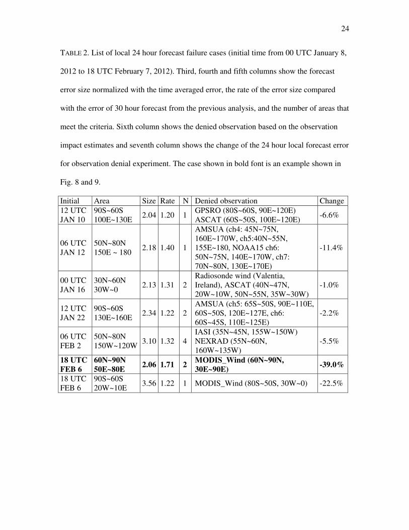
TABLE 2. List of local 24 hour forecast failure cases (initial time from 00 UTC January 8,

2012 to 18 UTC February 7, 2012). Third, fourth and fifth columns show the forecast

error size normalized with the time averaged error, the rate of the error size compared

with the error of 30 hour forecast from the previous analysis, and the number of areas that

meet the criteria. Sixth column shows the denied observation based on the observation

impact estimates and seventh column shows the change of the 24 hour local forecast error

for observation denial experiment. The case shown in bold font is an example shown in

Fig. 8 and 9.

Initial Area Size Rate N Denied observation Change

12 UTC

JAN 10

90S~60S

100E~130E 2.04 1.20 1

GPSRO (80S~60S, 90E~120E)

ASCAT (60S~50S, 100E~120E) -6.6%

06 UTC

JAN 12

50N~80N

150E ~ 180 2.18 1.40 1

AMSUA (ch4: 45N~75N,

160E~170W, ch5:40N~55N,

155E~180, NOAA15 ch6:

50N~75N, 140E~170W, ch7:

70N~80N, 130E~170E)

-11.4%

00 UTC

JAN 16

30N~60N

30W~0 2.13 1.31 2

Radiosonde wind (Valentia,

Ireland), ASCAT (40N~47N,

20W~10W, 50N~55N, 35W~30W)

-1.0%

12 UTC

JAN 22

90S~60S

130E~160E 2.34 1.22 2

AMSUA (ch5: 65S~50S, 90E~110E,

60S~50S, 120E~127E, ch6:

60S~45S, 110E~125E)

-2.2%

06 UTC

FEB 2

50N~80N

150W~120W 3.10 1.32 4

IASI (35N~45N, 155W~150W)

NEXRAD (55N~60N,

160W~135W)

-5.5%

18 UTC

FEB 6

60N~90N

50E~80E 2.06 1.71 2

MODIS_Wind (60N~90N,

30E~90E) -39.0%

18 UTC

FEB 6

90S~60S

20W~10E 3.56 1.22 1 MODIS_Wind (80S~50S, 30W~0) -22.5%

25

-3

-2.5

-2

-1.5

-1

-0.5

0

1/8 1/9 1/10 1/11 1/12 1/13 1/14 1/15

Err

or

red

uct

ion

in m

ois

t to

tal e

ne

rgy

[J

kg

-1]

Date (analysis time, UTC)

Total forecast error reduction

True Reduction

Estimate(Fixed)

Estimate(Advected)

Correlation(Fixed): 0.318

Correlation(Advected): 0.730

FIG. 1. Time series of the total forecast error reduction of each estimate (unit: J kg-1

).

Black, red, and blue lines show the actual forecast error reduction verified against the

own analysis, estimated error reduction from the EnKF-based method with fixed

localization (Fixed), and with moving localization (Advected). Numbers on upper left

corner show the correlation of each estimate to the actual forecast error reduction.

26

−0.7 −0.6 −0.5 −0.4 −0.3 −0.2 −0.1 0.0

Aircraft

Radiosonde

Satellite_Wind

GPSRO

Land−Surface

Marine−Surface

MODIS_Wind

ASCAT_Wind

PIBAL

NEXRAD_Wind

Profiler_Wind

Dropsonde

WINDSAT_Wind

TCVital

Ozone

AMSUA

IASI

Aqua_AIRS

ATMS

HIRS

MHS

GOES

SEVIRI

Moist total energy [J kg−1]

Average total observation impacts on 1 analysisa)

Satellite

Other

−6e−06 −5e−06 −4e−06 −3e−06 −2e−06 −1e−06 0 1e−06

Aircraft

Radiosonde

Satellite_Wind

GPSRO

Land−Surface

Marine−Surface

MODIS_Wind

ASCAT_Wind

PIBAL

NEXRAD_Wind

Profiler_Wind

Dropsonde−2.81e−05

WINDSAT_Wind

TCVital−2.24e−04

Ozone

AMSUA

IASI

Aqua_AIRS

ATMS

HIRS

MHS

GOES

SEVIRI

Moist total energy [J kg−1]

Average observation impacts per 1 observationb)

Satellite

Other

FIG. 2. Estimated average 24 hour forecast error reduction contributed from each

observation types (moist total energy, J kg-1

). a) represents the total error reduction and b)

represents error reduction per 1 observation.

27

−0.7 −0.6 −0.5 −0.4 −0.3 −0.2 −0.1 0.0

Aircraft

Radiosonde

Satellite_Wind

GPSRO

Land−Surface

Marine−Surface

MODIS_Wind

ASCAT_Wind

PIBAL

NEXRAD_Wind

Profiler_Wind

Dropsonde

WINDSAT_Wind

TCVital

Ozone

AMSUA

IASI

Aqua_AIRS

ATMS

HIRS

MHS

GOES

SEVIRI

Dry total energy [J kg−1]

Average total observation impacts on 1 analysisa)

Satellite

Other

−6e−06 −5e−06 −4e−06 −3e−06 −2e−06 −1e−06 0 1e−06

Aircraft

Radiosonde

Satellite_Wind

GPSRO

Land−Surface

Marine−Surface

MODIS_Wind

ASCAT_Wind

PIBAL

NEXRAD_Wind

Profiler_Wind

Dropsonde−2.54e−05

WINDSAT_Wind

TCVital−1.74e−04

Ozone

AMSUA

IASI

Aqua_AIRS

ATMS

HIRS

MHS

GOES

SEVIRI

Dry total energy [J kg−1]

Average observation impacts per 1 observationb)

Satellite

Other

FIG. 3. Same as Fig. 2 but with the dry total energy norm (J kg-1

).

28

FIG. 4. Estimated AIRS satellite radiance observation impacts classified by each channels

with the dry total energy (red, J kg-1

), and the moist total energy (blue, J kg-1

). Estimated

forecast error reduction by 1 observation is shown. Vertical bars represent the 95 %

confidence interval of the average values.

29

−7e−06

−6e−06

−5e−06

−4e−06

−3e−06

−2e−06

−1e−06

0

2000−950950−800 800−600 600−400 400−250 250−125 125−40 40−0

Observed level [hPa]M

ois

t to

tal energ

y [J k

g−

1]

Average impact per 1 obs (Radiosonde)a)

−7e−06

−6e−06

−5e−06

−4e−06

−3e−06

−2e−06

−1e−06

0

2000−950 950−800 800−600 600−400 400−250 250−125

Observed level [hPa]

Mois

t to

tal energ

y [J k

g−

1]

Average impact per 1 obs (Aircraft)b)

FIG. 5. Estimated average observation impacts of a) radiosonde and b) aircraft classified

by observed level (moist total energy, J kg-1

). Estimated forecast error reduction by 1

observation is shown.

30

FIG. 6. Average number of assimilated radiosonde observations a) from 250 to 125 hPa,

b) from 800 to 600 hPa and aircraft observations c) from 250 to 125 hPa and d) from 800

to 600 hPa in each 5o by 5

o area on 1 analysis.

31

FIG. 7. Average impact (moist total energy, J kg-1

) of 1 radiosonde profile from the fixed

land stations. Only the stations that have more than 20 profiles in the period are shown.

Numbers 4220 (Egedesminde) and 4270 (Narssassuaq) indicate the location of the

stations shown in Fig. 8 and 9.

32

33

FIG. 8. Comparison of the radiosonde observations from Narssassuaq (red line, 4270) and

Egedesminde (blue line, 4220) showing a) average impacts (J kg-1

) of each observation

element (solid: temperature, dashed: winds, dotted: humidity) on each pressure level by 1

profile and observation departure statistics (dashed: bias, solid: standard deviation) of b)

temperature (K) and c) wind speed (m s-1

).

34

FIG. 9. 24 hour forecast error of 500 hPa geopotential height (unit: m, 18 UTC February

6, 2012 initial) from original analysis (left) and forecast change due to the removal of the

observations (MODIS polar wind in 60N~90N, 30E~90E) in the data denial experiment

(middle: actual change and right: projection on the ensemble perturbations). Black

contours show the analysis. Magenta cones show the target area of the observation impact

estimate.