Diagnosing NCEP GFS

Forecast Errors

Fanglin Yang

Environmental Modeling Center

National Centers for Environmental Prediction

Camp Springs, Maryland, USA

THORPEX PDP/WGNE Workshop on "Diagnosis of Model Errors"

ETH, Zurich, 7-9 July 2010

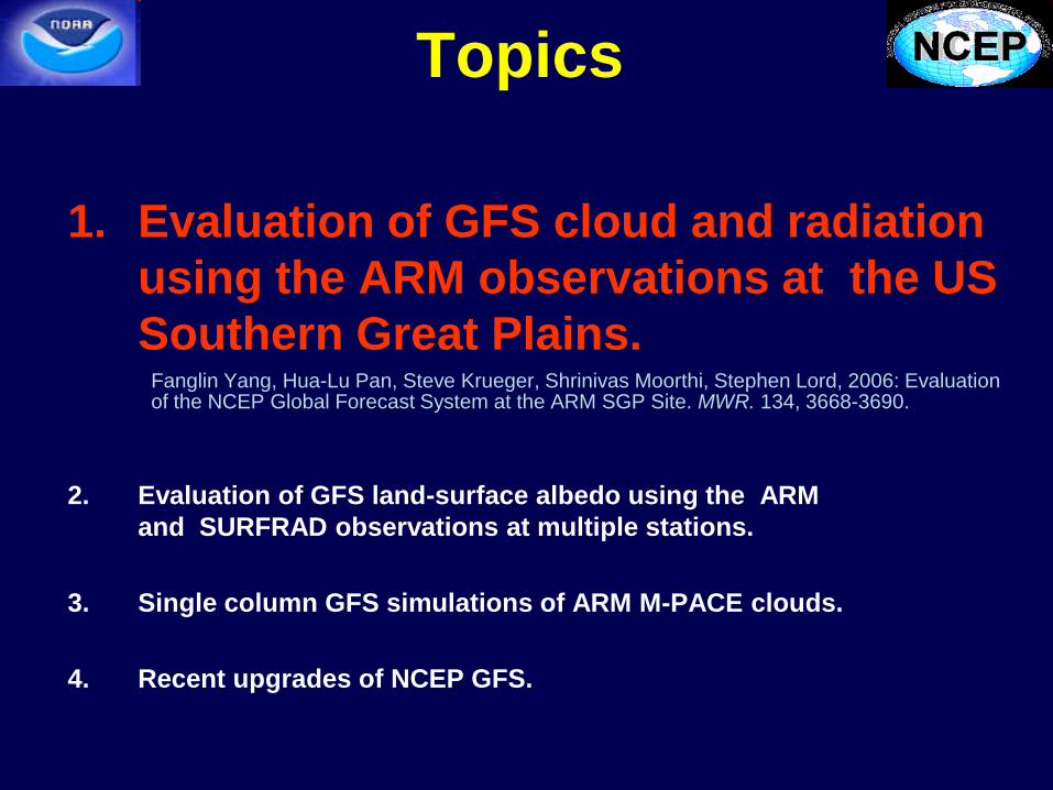
Topics

1. Evaluation of GFS cloud and radiation using ARM observations at the US Southern Great Plains.

2. Evaluation of GFS land-surface albedo using the ARM and SURFRAD observations at multiple stations.

3. Single column GFS simulation of ARM M-PACE clouds.

4. Recent upgrades of NCEP GFS.

Topics

1. Evaluation of GFS cloud and radiation

using the ARM observations at the US

Southern Great Plains. Fanglin Yang, Hua-Lu Pan, Steve Krueger, Shrinivas Moorthi, Stephen Lord, 2006: Evaluation of the NCEP Global Forecast System at the ARM SGP Site. MWR. 134, 3668-3690.

2. Evaluation of GFS land-surface albedo using the ARM

and SURFRAD observations at multiple stations.

3. Single column GFS simulations of ARM M-PACE clouds.

4. Recent upgrades of NCEP GFS.

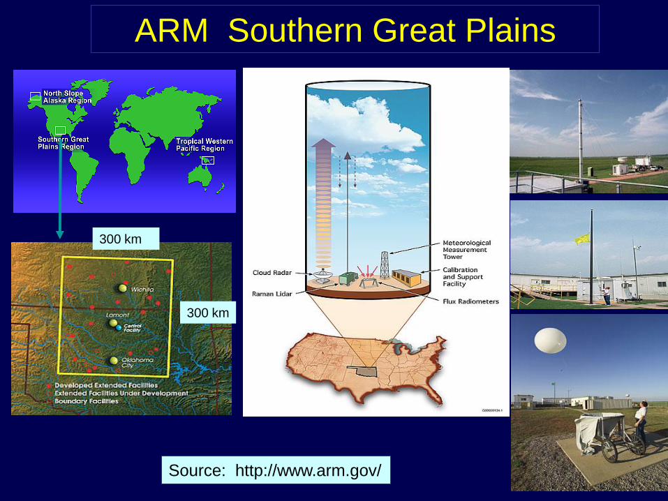
ARM Southern Great Plains

300 km

300 km

Source: http://www.arm.gov/

GFS Forecasts and ARM Observations

NCEP Global Forecast System

GFS Single-column output from 2002 through 2004 for the ARM stations, archived at a 3-hour interval up to 48 hours of forecasts.

ARM data

Stream

Variables Interval &

Sites

sgp30smosE*.

b1

Surface Meteorological Observations

wind speed and direction at 10 m;

Ts and RH at 2 m;

Ps at 1 m; Precipitation; Snow depth

30 minutes;

16 EF

sgp30ebbrE*.b

1

Energy Balance Bowen Ratio

sensible, latent and ground heat fluxes (~ 10 W/m2

accuracy); Soil moisture.

30 minutes;

14 EF

sgpsirsE*.b1 Solar Infrared Radiation Station

irradiances of surface solar (0.3-3 um, ~10 W/m2 )

and longwave radiation(4-50 um; ~2 W/m2 )

1 minute;

22 EF and

C1

sgpbeflux1lon

gC1.c1

VAP: Best-Estimate Radiative Flux

broadband irradiances of surface solar and

longwave radiation

1 minute;

C1/E13

sgpmwrprofC1

.c1

VAP: MWR, RASS and SMOS Retrievals

water vapor and temperature profiles (250 m

resolution); columnar precipitable and could liquid

water; cloud base height.

1 hour;

C1

sgparsclbnd1c

lothC1.c1

Active Remotely-Sensed Clouds Locations

Base and top cloud boundary info. from MMCR,

ceilometer, lidar data

10 seconds

C1

All ARM data were processed to match 3-hourly GFS output

A Scale-Dependence Test

GFS Resolution:

• T254: ~ 55km

Q: How many stations of ARM observations to use?

• Single station at CF/E13 (data rich)?

• Mean over an area comparable to the model grid, like the red rectangular?

• Or mean over the entire SGP site?

ARM SGP Sites, 300km x 300kmCF – Central Facility

EF – Extended Facility

BF – Boundary Facility

OB1

OB2

OB3

model biases (FCST-OB1) >> [OB2 - OB1] << [OB3 - OB1]

The difference between OB2 and OB1 is much smaller than fcst errors; It is

reasonable to use the SGP CF point observations to represent the conditions

over the GFS model grid (see more details in Yang et al. 2006).

SW

LW

Surface Energy Fluxes, 2003-2004 Mean Diurnal Cycle

3 PM

• Overestimate surface downward SW and LH (cloud bias)

• Underestimate daytime SH and overestimate nighttime SH (surface roughness bias)

• Underestimate surface downward LW, shifted diurnal cycle (a scaling issue)

3 PM

Down SW

UP SW

Down LW

SH

T2m

LH

GFSARM

Surface Energy Fluxes (3 PM Local Time) at SGP CF

SD

SW

SU

SW

SD

LW

SU

LWLH SH GH NET

ARM 581 - 120 343 - 437 - 167 - 174 - 28 - 2

GFS 625 - 119 329 - 424 - 243 - 130 - 34 4

GFS-ARM 44 1 - 14 13 - 76 44 - 6 6

• Underestimate surface albedo

• Overestimate surface

downward SW and LH

• Underestimate daytime SH

and overestimate nighttime SH

The model attained

surface radiative balance

by error cancelation

among SW, LH and SH.

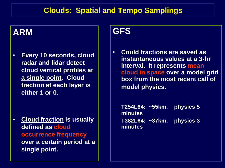
Clouds: Spatial and Tempo Samplings

ARM

• Every 10 seconds, cloud

radar and lidar detect

cloud vertical profiles at

a single point. Cloud

fraction at each layer is

either 1 or 0.

• Cloud fraction is usually

defined as cloud

occurrence frequency

over a certain period at a

single point.

GFS

• Could fractions are saved as instantaneous values at a 3-hr interval. It represents mean cloud in space over a model grid box from the most recent call of

model physics.

T254L64: ~55km, physics 5 minutes

T382L64: ~37km, physics 3 minutes

Cloud Fraction and Total Cloud Amount

ARM ARSCL: cloud occurrence frequency computed using

10-s data in the last 5 minutes of each 3-hour period (top), all

data in each 3-hour period (middle). Under-sampled in space.

GFS: 12-36-hr forecasts of cloud fraction from model last call

of physics (5-minute time step) in each 3 hour period. Under-

sampled in time.

Random overlap, 10-day running mean total

cloud amount.

Sampling Uncertainty

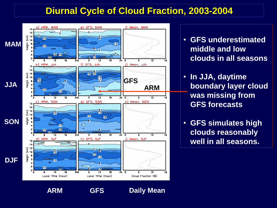
• GFS underestimated

middle and low

clouds in all seasons

• In JJA, daytime

boundary layer cloud

was missing from

GFS forecasts

• GFS simulates high

clouds reasonably

well in all seasons.

GFSARM

Diurnal Cycle of Cloud Fraction, 2003-2004

MAM

JJA

SON

DJF

ARM GFS Daily Mean

• For both ARM and

GFS, precipitating

clouds dominate in the

middle and lower

troposphere.

• GFS failed to simulate

boundary-layer non-

precipitating clouds.

• GFS underestimated

precipitating clouds in

the lower troposphere

GFSARM

Diurnal Cycle of Cloud Fraction: precipitating v.s. non-precipitating

JJA W/O

Precip

JJA W/

Precip

DJF W/O

Precip

DJF W

Precip

ARM GFS Daily Mean

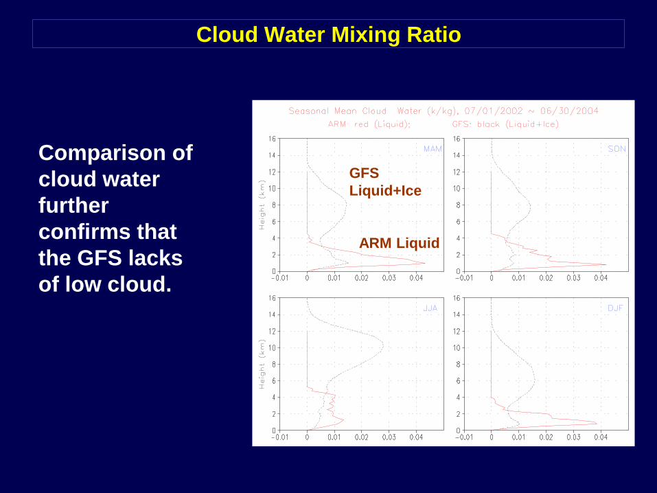
Cloud Water Mixing Ratio

GFS

Liquid+Ice

ARM Liquid

Comparison of

cloud water

further

confirms that

the GFS lacks

of low cloud.

Summary I

• Sampling of ARM observations differs from NWP

models in space and time. Cautions must be

exercised for proper comparison and validation.

• GFS cloud fraction at the ARM SGP CF site was

generally underestimated at all layers except for

high cirrus clouds. Underestimate of clouds led to

overestimate of surface downward shortwave fluxes.

• Diurnal cycle of GFS low clouds was incorrect. GFS

failed to simulate non-precipitating low clouds. A new

shallow-convection scheme based on SAS developed by Han and Pan (2010) will be

implemented in the GFS in August 2010 to the replace the current Tiedtke diffusion

scheme in operational GFS.

Topics

1. Evaluation of GFS cloud and radiation using the ARM observations at

the US Southern Great Plains Fanglin Yang, Hua-Lu Pan, Steve Krueger, Shrinivas Moorthi, Stephen Lord, 2006: Evaluation of the NCEP Global Forecast System at the ARM SGP Site. MWR. 134, 3668-3690.

2. Evaluation of GFS land-surface albedo

using the ARM and SURFRAD

observations at multiple stations.Fanglin Yang, Kenneth Mitchell, Yu-Tai Hou, Yongjiu Dai, Xubin Zeng, Zhou Wang, and Xin-Zhong

Liang, 2008: Dependence of land surface albedo on solar zenith angle: observations and model

parameterizations. Journal of Applied Meteorology and Climatology. No.11, Vol 47, 2963-2982.

3. Single column GFS simulations of ARM M-PACE clouds.

4. Recent upgrades of NCEP GFS

ARM

GFS

GFS underestimated surface albedo at the ARM SGP CF site

Objectives

1. Use field observations to assess the accuracy of land surface-albedo parameterization in NCEP GFS.

2. Develop new parameterizations to better describe thedependence of snow-free land surface albedo on solarzenith angle for NWP and climate models.

US DOE

ARM SitesUS NOAA

SURFRAD Sites

Field Observations

Variables: surface downward SW total flux, surface downward SW

direct-beam flux, upward SW total flux, solar zenith angle

(SZA), cloud cover.

Time: 1997-2004 (for most stations), three-minute mean samples,

snow-free days.

XSGP

Manus &

Nauru

dirSW

dirSW

clouds

diffSW

diffSW

particles

ARM and

SURFRAD

Measured:

totalSW

dirSW

dirSW

dirdirdir SWSW diffdiffdiff SWSW

Still need:

totalSW

dirtotaldiff SWSWSW

Question?

How to partitioning

the upward total into

upward direct and

upward diffuse?

NCEP GFS uses different surface albedos for direct and diffuse SW fluxes

diffSW

Methodology

1. Compute monthly mean albedo for diffuse fluxes using a subgroupof samples that satisfy two conditions: overcast and more than 99%downward fluxes are diffuse. The resultant diffuse-beam albedosare assumed to be applicable for all samples in subsequent analyses.

2. Apply the diffuse albedo to ALL samples to divide the upward fluxinto two parts, one associated with the downward direct beam andthe other associated with the downward diffuse flux.

3. Derive direct-beam albedo for all samples and monthly mean direct-beam albedo at SZA=60o.

4. Empirically fit the ARM and SURFRAD data to obtain thedependence of normalized direct-beam albedo as a function of SZA.

5. Compare the fits with the model parameterizations

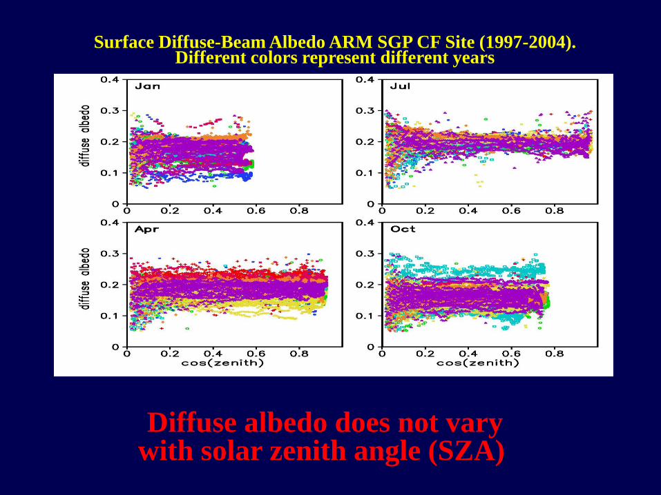
Surface Diffuse-Beam Albedo ARM SGP CF Site (1997-2004). Different colors represent different years

Diffuse albedo does not vary with solar zenith angle (SZA)

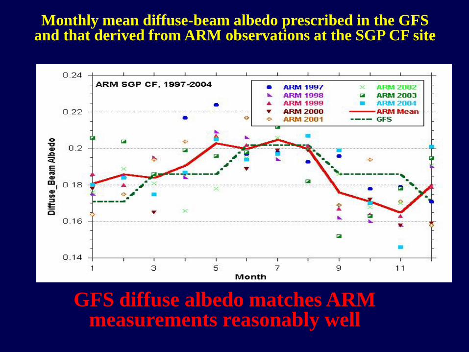
Monthly mean diffuse-beam albedo prescribed in the GFS and that derived from ARM observations at the SGP CF site

GFS diffuse albedo matches ARM measurements reasonably well

Direct-beam albedos derived from ARM observationsThe crosses (squares) represent albedos derived from observations in the morning (afternoon).

Direct-beam albedo is a strong function of SZA

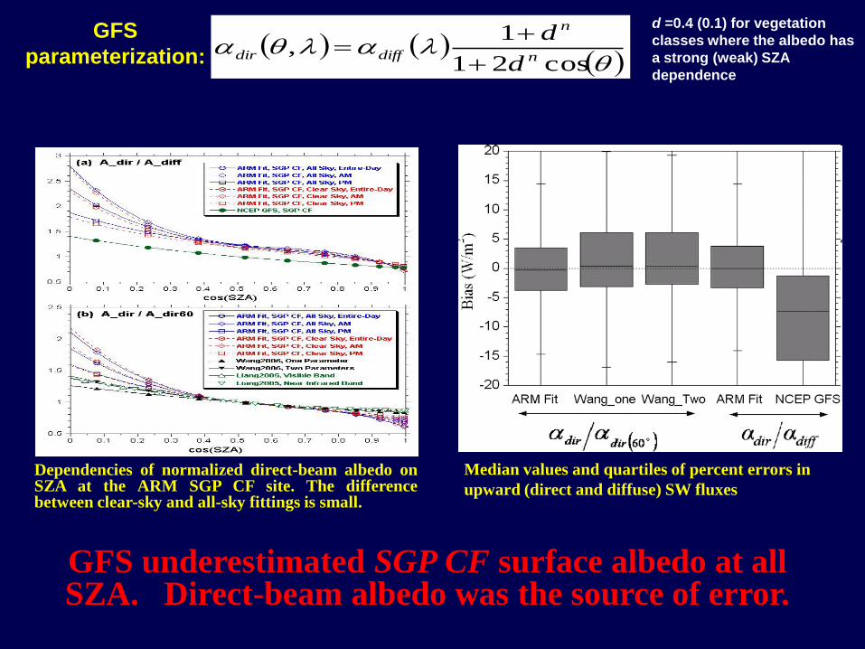
Dependencies of normalized direct-beam albedo onSZA at the ARM SGP CF site. The differencebetween clear-sky and all-sky fittings is small.

Median values and quartiles of percent errors in

upward (direct and diffuse) SW fluxes

GFS underestimated SGP CF surface albedo at all SZA. Direct-beam albedo was the source of error.

cos21

1,

n

n

diffdird

d

GFS

parameterization:

d =0.4 (0.1) for vegetation

classes where the albedo has

a strong (weak) SZA

dependence

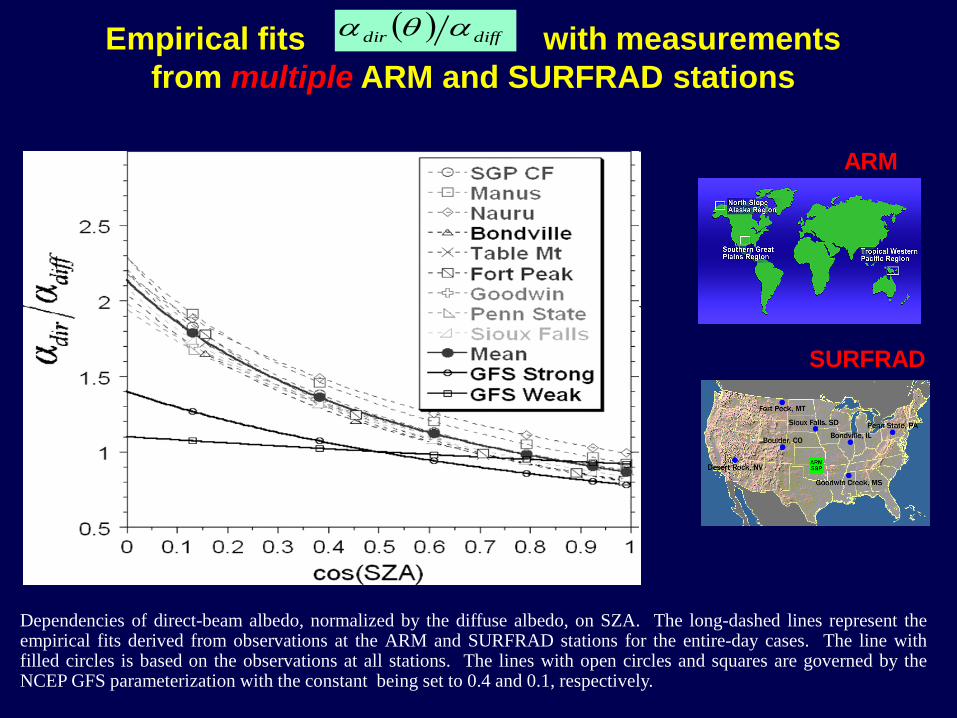
Dependencies of direct-beam albedo, normalized by the diffuse albedo, on SZA. The long-dashed lines represent theempirical fits derived from observations at the ARM and SURFRAD stations for the entire-day cases. The line withfilled circles is based on the observations at all stations. The lines with open circles and squares are governed by theNCEP GFS parameterization with the constant being set to 0.4 and 0.1, respectively.

Empirical fits with measurements

from multiple ARM and SURFRAD stations

ARM

SURFRAD

diffdir

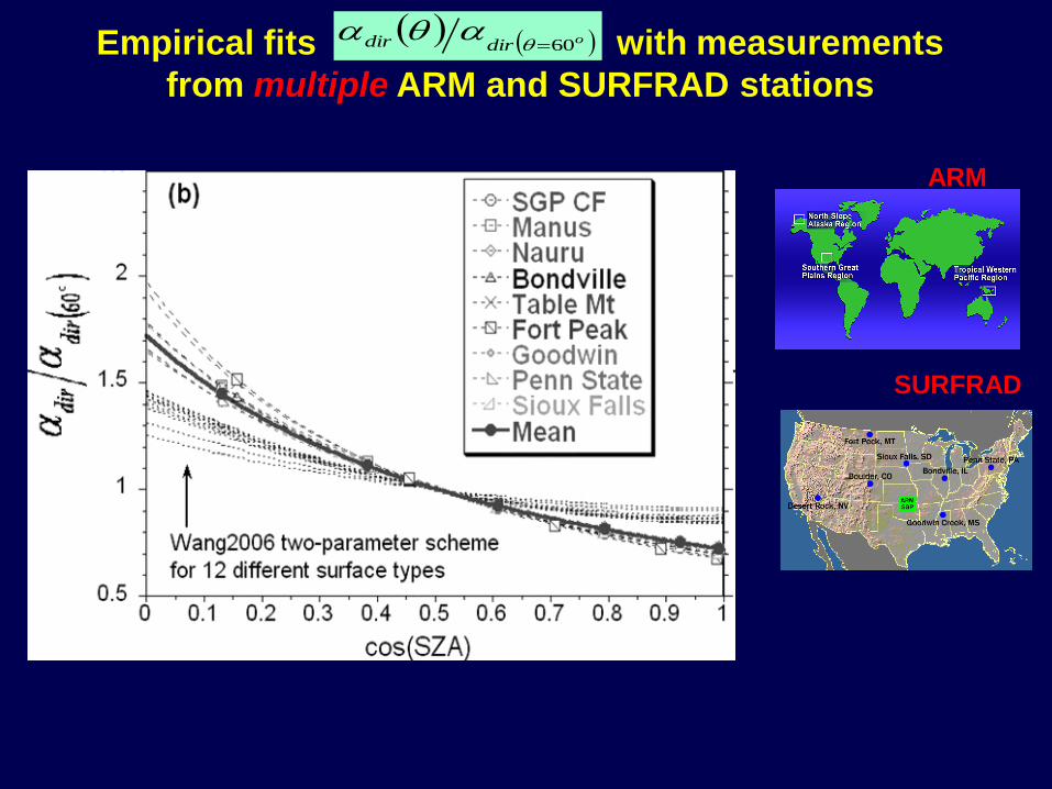
Empirical fits with measurements

from multiple ARM and SURFRAD stations

ARM

SURFRAD

odirdir 60

Empirical fits using data from observations at all

ARM and SURFRAD stations

32

1 cos34.2cos92.4cos02.427.2,

mn

diff

mn

dirf

32

2 cos02.2cos13.4cos34.389.1,60

,

omn

dir

mn

dirf

Included in the next GFS implementation

Alternatively, keep current GFS parameterizations, but with updated coefficients

cos48.11

14.11,1

mn

diff

mn

dirf

cos55.11

775.01

,60

,2

omn

dir

mn

dirf

New polynomial fits

1. Compared to the ARM and SURFRAD observations, the

NCEP GFS parameterization underestimated direct-beam

albedo at all solar zenith angles.

2. The surface types of the ARM and SURFRAD sites are

different; however, the differences among the fits for the

dependences of the normalized direct-beam albedo on SZA

derived from these sites are relatively small.

3. The empirical fits obtained from this study have been

included in the upcoming Q3FY2010 GFS implementation.

Summary II

Topics

1. Evaluation of GFS cloud and radiation using the ARM observations at

the US Southern Great Plains Fanglin Yang, Hua-Lu Pan, Steve Krueger, Shrinivas Moorthi, Stephen Lord, 2006: Evaluation of the NCEP Global Forecast System at the ARM SGP Site. MWR. 134, 3668-3690.

2. Evaluation of GFS land-surface albedo using the ARM

and SURFRAD observations at multiple stations.Fanglin Yang, Kenneth Mitchell, Yu-Tai Hou, Yongjiu Dai, Xubin Zeng, Zhou Wang, and Xin-Zhong Liang, 2008: Dependence of land

surface albedo on solar zenith angle: observations and model parameterizations. Journal of Applied Meteorology and Climatology.

No.11, Vol 47, 2963-2982.

3. Single column GFS simulations of

ARM M-PACE clouds.

4. Recent upgrades of NCEP GFS

M-PACE

DOE ARM Mixed-Phase Arctic Cloud Experiment

• 27 Sept ~ 22 October, 2004

• Northern Alaska and adjacent

Arctic Ocean

• Measurements were made from

both in-situ and remote (aircraft)

sensors.

Citation ProteusAerosonde Payloads

Credit: Hans Verlinde

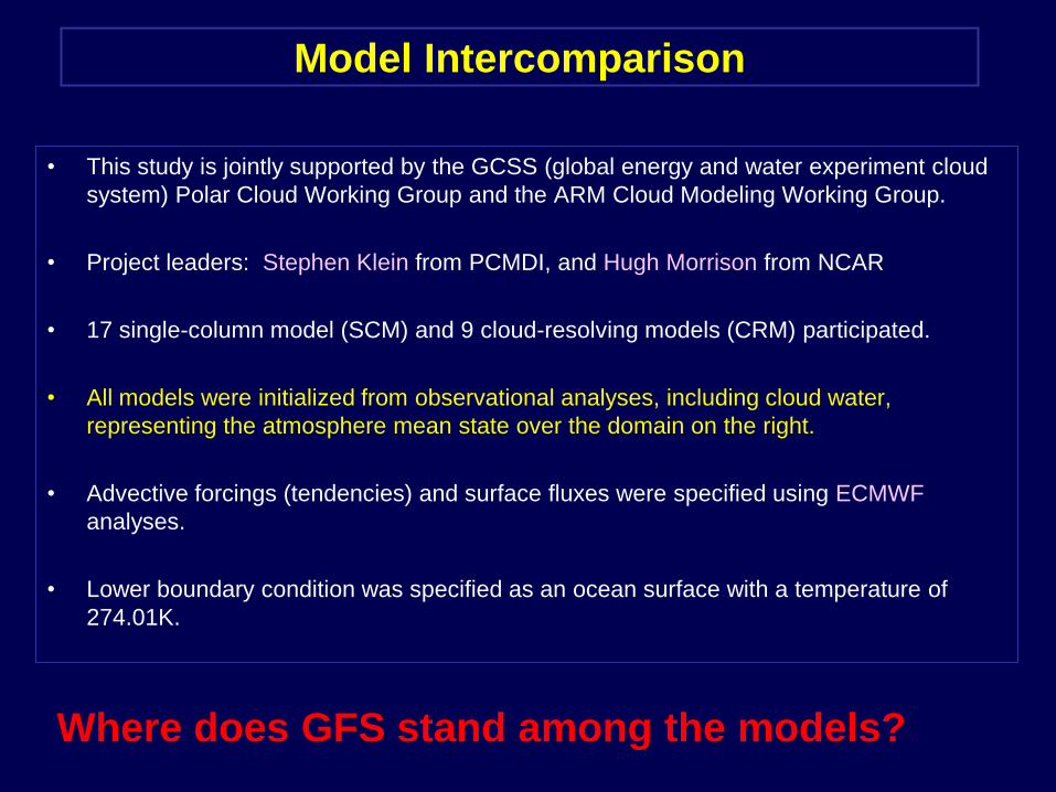
Model Intercomparison

• This study is jointly supported by the GCSS (global energy and water experiment cloud

system) Polar Cloud Working Group and the ARM Cloud Modeling Working Group.

• Project leaders: Stephen Klein from PCMDI, and Hugh Morrison from NCAR

• 17 single-column model (SCM) and 9 cloud-resolving models (CRM) participated.

• All models were initialized from observational analyses, including cloud water,

representing the atmosphere mean state over the domain on the right.

• Advective forcings (tendencies) and surface fluxes were specified using ECMWF

analyses.

• Lower boundary condition was specified as an ocean surface with a temperature of

274.01K.

Where does GFS stand among the models?

NCEP GFS SCM

• The NCEP SCM was built based on the 2006 version of the GFS

• Two SCM versions, 64 and 640 vertical layers, were run with and without ice microphysics.

• Operational GFS forecasts in October 2004 were used to derive vertical profiles/soundings at the M-PACE sites.

17 Participating SCMs

Single

Moment with

T-Dependence

01

0/1

0

T

TTiTiT

TiT

fwater

CTi o17

CTi o60

CTi o20

CTi o88

CTi o88

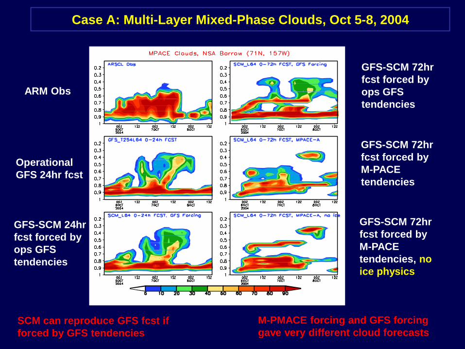
Case A: Multi-Layer Mixed-Phase Clouds, Oct 5-8, 2004

Operational

GFS 24hr fcst

ARM Obs

GFS-SCM 24hr

fcst forced by

ops GFS

tendencies

GFS-SCM 72hr

fcst forced by

ops GFS

tendencies

GFS-SCM 72hr

fcst forced by

M-PACE

tendencies

GFS-SCM 72hr

fcst forced by

M-PACE

tendencies, no

ice physics

SCM can reproduce GFS fcst if

forced by GFS tendencies

M-PMACE forcing and GFS forcing

gave very different cloud forecasts

LWP (g/m2) IWP (g/m2)

Mean ARM Retrieval 119 81

17-SCM Median 123 42

GFS SCM 30 36

Case A: Multi-Layer Mixed-Phase Clouds, Oct 5-8, 2004

• For All Models: reasonable LWP simulation; strongly

underestimated IWP with large spread among the models.

• NCEP GFS-SCM: largely underestimated LWP;

underestimated IWP as did other models.

• Models employing simple microphysics schemes with temperature-based partitioning of

the cloud liquid and ice masses are not able to produce results consistent with

observations. Models with a more sophisticated, two-moment treatment of the cloud

microphysics produce a somewhat smaller liquid water path that is closer to observations.

Case B: Single Layer Mixed-Phase

Stratocumulus, Oct 9-10, 2004

MODIS composite, October 9, 2004.

The boundary layer clouds occurred when cold air above the sea ice to the northeast of Alaska flowed over the ice-

free Beaufort Sea inducing the significant surface heat fluxes responsible for cloud formation. The sea ice is visible in

the upper right corner of the image. The clouds were observed in the northeasterly flow between the ARM stations of

Barrow and Oliktok Point on the coast of snow-covered Alaska. As is common in “cold-air outbreak” stratocumulus,

boundary layer “rolls” or “cloud streets” developed with a horizontal scale that increases in the downstream direction.

Barrow

Oliktok Point

LWP IWP

ARM Mean

(flight & ground)150 22

All 17-SCM Median 56 29

SCMs With single moment 21 34

NCEP GFS SCM 16 39

Case B: Single Layer Mixed-Phase Stratocumulus

• Observation: a well-mixed boundary layer with a cloud top

temperature of –15 oC, dominant by water cloud.

• All Models: underestimated LWP; IWP is close to the obs.

•

• NCEP GFS-SCM: compared to other models, GFS tends to

have even lower LWP; GFS IWP is more realistic.

Summary III

• Model simulations have large spread. No single factor is found to lead a good or bad simulation.

• However, models with more sophisticated microphysics are somewhat better, but really not much.

• NCEP GFS-SCM: tends to produce less LWP than other models. GFS LWP is underestimated for both case A and B. Most models overestimated for case A. GFS IWP is not much different from others.

• Should the T-dependent partitioning of LWP and IWP in the GFS be tuned?Earlier studies (Curry 200; McFarquhar &Cober 2004) showed that , unlike the mid-latitude cloud, Arctic mixed-phase cloud has little temperature dependence for the amount of LWP versus IWP.

• No consensus among models. It is still a challenge for models to capture Arctic mixed-phase clouds.

Topics

1. Evaluation of GFS cloud and radiation using the ARM

observations at the US Southern Great Plains Fanglin Yang, Hua-Lu Pan, Steve Krueger, Shrinivas Moorthi, Stephen Lord, 2006: Evaluation of the NCEP Global Forecast System at the ARM SGP Site. MWR. 134, 3668-3690.

2. Evaluation of GFS land-surface albedo using the ARM

and SURFRAD observations at multiple stations.Fanglin Yang, Kenneth Mitchell, Yu-Tai Hou, Yongjiu Dai, Xubin Zeng, Zhou Wang, and Xin-Zhong Liang,

2008: Dependence of land surface albedo on solar zenith angle: observations and model parameterizations.

Journal of Applied Meteorology and Climatology. No.11, Vol 47, 2963-2982.

3. Single column GFS simulations of ARM M-PACE clouds.

4. Recent upgrades of NCEP GFS

Q3FY2010 GFS Implementation: Major Changes

• Resolution and ESMF– T382L64 to T574L64 for fcst1 (0-192hr) & T190L64 for fcst2 (192-384 hr) .

– ESMF 3.1.0rp2

• Radiation and cloud– Changing SW routine from ncep0 to RRTM2

– Changing longwave computation frequency from three hours to one hour

– Adding stratospheric aerosol SW and LW and tropospheric aerosol LW

– Changing aerosol SW single scattering albedo from 0.90 in the operation to 0.99

– Changing SW aerosol asymmetry factor. Using new aerosol climatology.

– Changing SW cloud overlap from random to maximum-random overlap

– Using time varying global mean CO2 instead of constant CO2 in the operation

– Using the Yang et al. (2008) scheme to treat the dependence of direct-beam surface albedo on solar zenith angle over snow-free land surface

• Removal of negative water vapor– Using a positive-definite tracer transport scheme in the

vertical to replace the operational central-differencing scheme to eliminate computationally-induced negative tracers.

– Changing GSI factqmin and factqmax parameters to reduce negative water vapor and supersaturation points from analysis step.

– Modifying cloud physics to limit the borrowing of water vapor that is used to fill negative cloud water to the maximum amount of available water vapor so as to prevent the model from producing negative water vapor.

– Changing the minimum value of water vapor mass mixing ratio in radiation from 1.0e-5 in the operation to 1.0e-20. Otherwise, the model artificially injects water vapor in the upper atmosphere where water vapor mixing ratio is often below 1.0e-5.

Q3FY2010 GFS Implementation: Major Changes

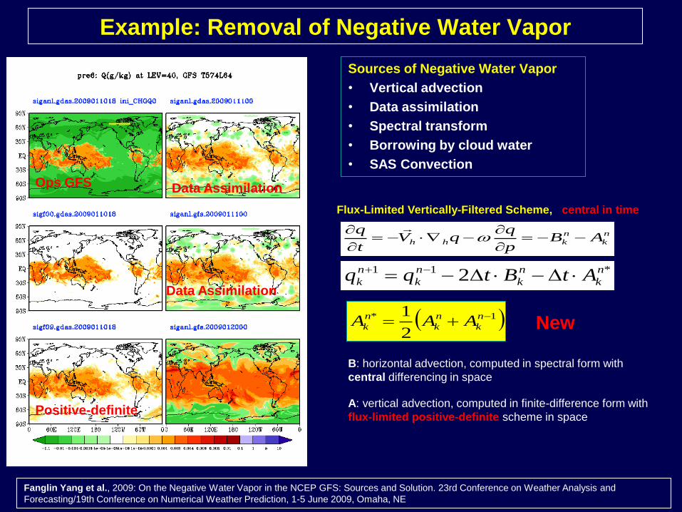
Example: Removal of Negative Water Vapor

Fanglin Yang et al., 2009: On the Negative Water Vapor in the NCEP GFS: Sources and Solution. 23rd Conference on Weather Analysis and

Forecasting/19th Conference on Numerical Weather Prediction, 1-5 June 2009, Omaha, NE

Sources of Negative Water Vapor

• Vertical advection

• Data assimilation

• Spectral transform

• Borrowing by cloud water

• SAS Convection

Ops GFS

_

Positive-definite

Data Assimilation

A: vertical advection, computed in finite-difference form with

flux-limited positive-definite scheme in space

Flux-Limited Vertically-Filtered Scheme, central in time

1*

2

1 n

k

n

k

n

k AAA New

n

k

n

khh ABp

qqV

t

q

*11 2 n

k

n

k

n

k

n

k AtBtqq

B: horizontal advection, computed in spectral form with

central differencing in space

Data Assimilation

• New mass flux shallow convection scheme (Han & Pan 2010)

– Use a bulk mass-flux parameterization same as deep convection scheme

– Separation of deep and shallow convection is determined by cloud depth (currently 150 mb)

– Entrainment rate is given to be inversely proportional to height (which is based on the LES studies) and much smaller than that in the deep convection scheme

– Mass flux at cloud base is given as a function of the surface buoyancy flux (Grant, 2001), which contrasts to the deep convection scheme using a quasi-equilibrium closure of Arakawa and Shubert (1974) where the destabilization of an air column by the large-scale atmosphere is nearly balanced by the stabilization due to the cumulus

• Revised deep convection scheme (Han & Pan 2010)

– Random cloud top selection in the current operational scheme is replaced by an entrainment rate parameterization with the rate dependent upon environmental moisture

– Include the effect of convection-induced pressure gradient force to reduce convective momentum transport (reduced about half)

– Trigger condition is modified to produce more convection in large-scale convergent regions but less convection in large-scale subsidence regions

– A convective overshooting is parameterized in terms of the convective available potential energy (CAPE)

Q3FY2010 GFS Implementation: Major Changes

• Revised Boundary Layer Scheme (Han & Pan 2010)

– Include stratocumulus-top driven turbulence mixing based on Lock et al.‟s (2000) study

– Enhance stratocumulus top driven diffusion when the condition for cloud top entrainment instability is met

– Use local diffusion for the nighttime stable PBL rather than a surface layer stability based diffusion profile

– Background diffusivity for momentum has been substantially increased to 3.0 m2s-1 everywhere, which helped reduce the wind forecast errors significantly

• Hurricane relocation

– Running hurricane relocation at the 1760x880 forecast grid instead of the 1152x576 analysis grid

– Posting GDAS pgb files first on Guassian grid (1760x880), then convert to 0.5-deg for hurricane relocation.

Q3FY2010 GFS Implementation: Major Changes

Ops GFS New shallow

convection scheme

Heating by Shallow Convection

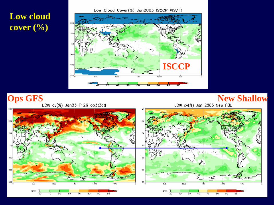
ISCCP

Ops GFS New Shallow

Low cloud

cover (%)

Marine Stratus

Tropical Wind RMSE

2008

2009

850 hPa

850 hPa

Significant reduction in tropical wind RMSE

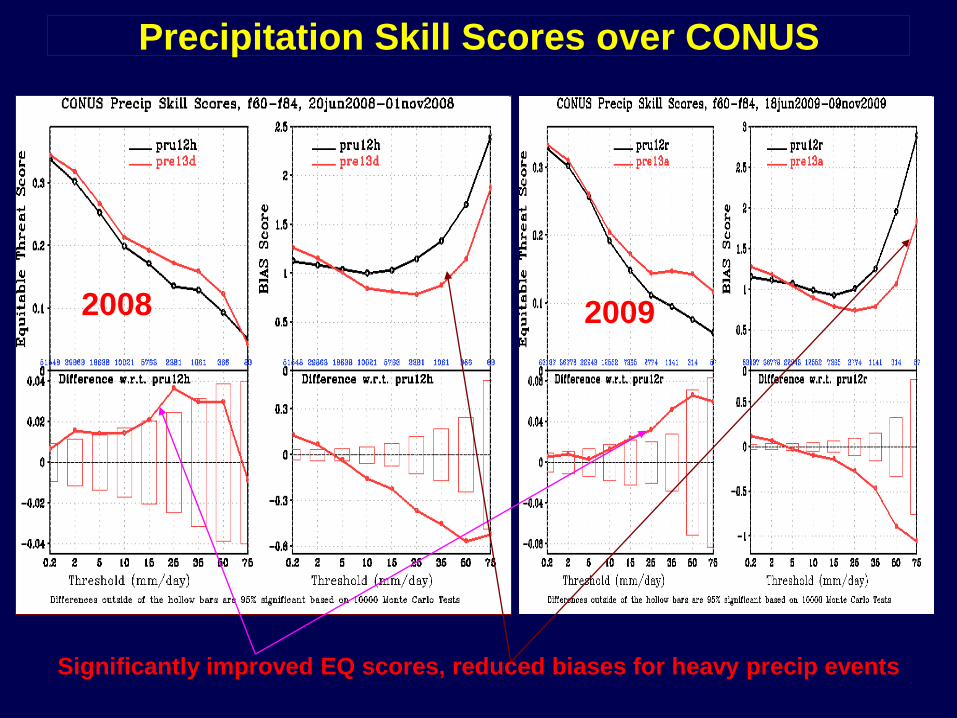
Precipitation Skill Scores over CONUS

2008 2009

Significantly improved EQ scores, reduced biases for heavy precip events

Hurricane Track and Intensity: 2008

Atlantic Track

Reduced track errors in both basins, significantly improved intensity forecast

Atlantic Intensity

East Pacific Track

East Pacific Intensity

T574

T382

Hurricane Track and Intensity: 2009

Atlantic Track

Reduced track error in East Pacific,

significantly improved intensity forecast in both basins.

Atlantic Intensity

East Pacific Track

East Pacific Intensity

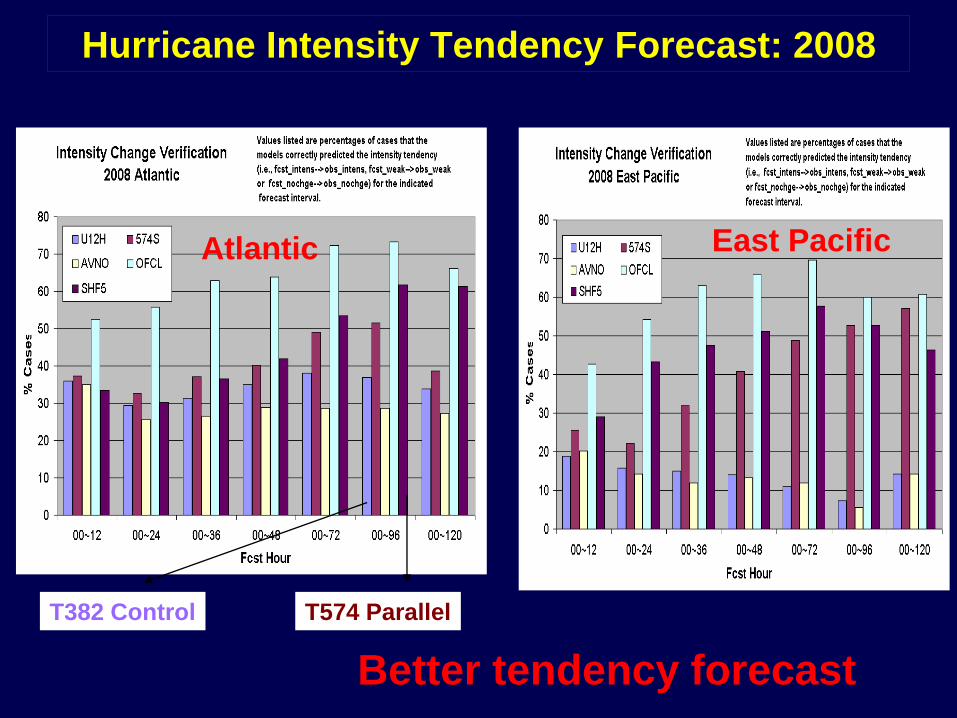
Hurricane Intensity Tendency Forecast: 2008

Better tendency forecast

Atlantic East Pacific

T382 Control T574 Parallel

Summary IV

The upcoming T574L64 implementation in

July 2010 is expected to be a major

improvement upon the current operational

T382L64 GFS in terms of height AC, wind

RMSE, precipitation skill score, and

hurricane track and intensity.

However, there are still a few remaining issues.

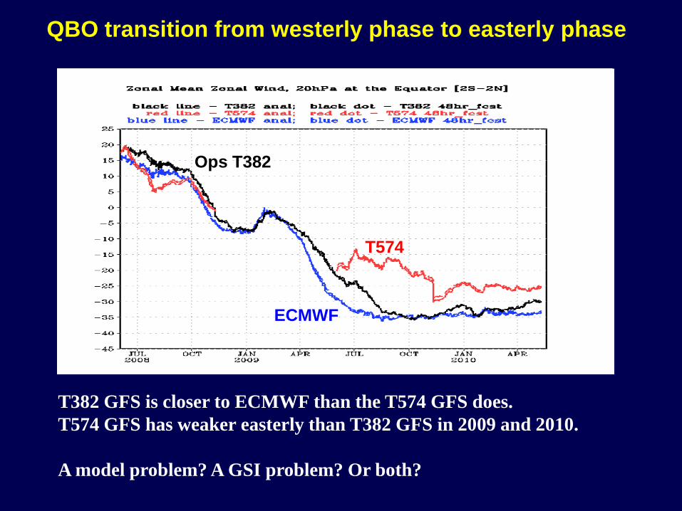
T382 GFS is closer to ECMWF than the T574 GFS does.

T574 GFS has weaker easterly than T382 GFS in 2009 and 2010.

A model problem? A GSI problem? Or both?

T574

ECMWF

Ops T382

QBO transition from westerly phase to easterly phase

Larger height RMS in the lower stratosphere,

likely caused by to small a minimum value of water vapor mixing ratio (1.0E-20)

• SL91 is

expensive.

• SL64 still has

problem. Noise

develops in the

upper

atmosphere

after a few days

of forecast

T878 L64 or L91 (~23 km) Semi- Lagrangian GFS

Near Future Updates

Extra slides

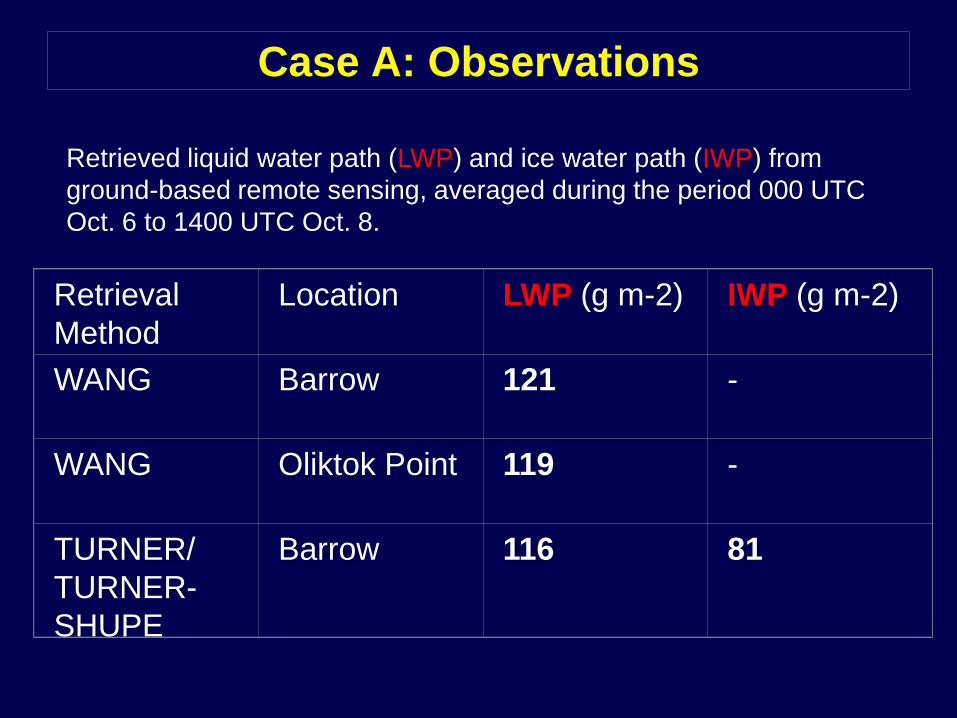
Retrieval

Method

Location LWP (g m-2) IWP (g m-2)

WANG Barrow 121 -

WANG Oliktok Point 119 -

TURNER/

TURNER-

SHUPE

Barrow 116 81

Case A: Observations

Retrieved liquid water path (LWP) and ice water path (IWP) from

ground-based remote sensing, averaged during the period 000 UTC

Oct. 6 to 1400 UTC Oct. 8.

Case A: Model Simulations

Modeled liquid water

path (LWP) and ice

water path (IWP) for the

baseline and sensitivity

tests with no ice

microphysics and

increased vertical

resolution. „1-M T-dep‟,

„1-M Ind‟, and „2-M‟ refer

to the models using one-

moment microphysics

schemes with T-

dependent partitioning,

one-moment schemes

with independent liquid

and ice, and two-

moment schemes,

respectively. Asterisk (*)

indicates models that

did not include

precipitation ice. Median

IWP values are derived

only from models that

include both cloud and

precipitation ice.

Model/Ensemble LWP (g m-2) IWP (g m-2)

Baseline High

Res

No Ice Baselin

e

High

Res

Median model 123 125 332 42 43

Median SCM 123 121 452 42 48

Median CRM 126 128 230 38 34

Median 1-M T-dep 147 127 332 48 49

Median 1-M Ind 123 172 693 42 63

Median 2-M 115 117 230 27 26

ARCSCM 199 197 452 28 26

CCCMA 182 220 216 62 83

ECHAM 93 166 97 1.9* 1.7*

GFDL 65 102 717 42 42

GISS 109 - - 37* -

McRAS 83 128 332 3.5* 4.5*

McRASI 44 81 504 5.8* 18*

NCEP 30 27 87 36 34SCAM3 298 334 - 42 55

SCAM3-MG 136 - - 21 -

SCAM3-LIU 155 105 - 87 121

SCRIPPS 245 162 668 20* 22*

UWM 123 103 1448 36 31

RAMS-CSU 170 184 215 13 20

SAM 211 125 793 54 43

UCLA-LARC 82 117 245 49 51

METO 26 20 180 26 25

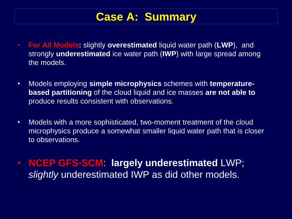
Case A: Summary

• For All Models: slightly overestimated liquid water path (LWP), and

strongly underestimated ice water path (IWP) with large spread among

the models.

• Models employing simple microphysics schemes with temperature-

based partitioning of the cloud liquid and ice masses are not able to

produce results consistent with observations.

• Models with a more sophisticated, two-moment treatment of the cloud

microphysics produce a somewhat smaller liquid water path that is closer

to observations.

• NCEP GFS-SCM: largely underestimated LWP;

slightly underestimated IWP as did other models.

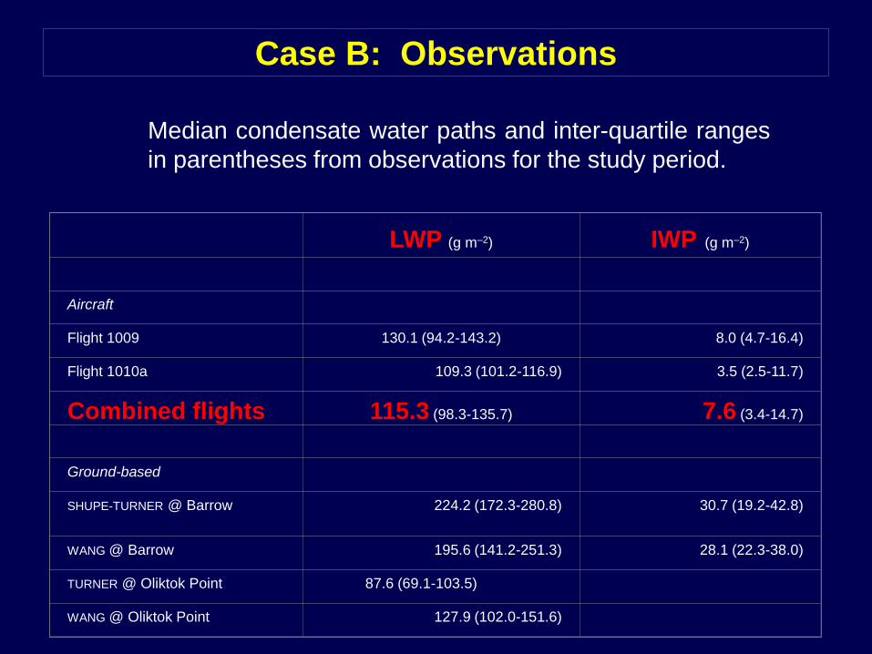
Case B: Observations

Median condensate water paths and inter-quartile ranges

in parentheses from observations for the study period.

LWP (g m–2) IWP (g m–2)

Aircraft

Flight 1009 130.1 (94.2-143.2) 8.0 (4.7-16.4)

Flight 1010a 109.3 (101.2-116.9) 3.5 (2.5-11.7)

Combined flights 115.3 (98.3-135.7) 7.6 (3.4-14.7)

Ground-based

SHUPE-TURNER @ Barrow 224.2 (172.3-280.8) 30.7 (19.2-42.8)

WANG @ Barrow 195.6 (141.2-251.3) 28.1 (22.3-38.0)

TURNER @ Oliktok Point 87.6 (69.1-103.5)

WANG @ Oliktok Point 127.9 (102.0-151.6)

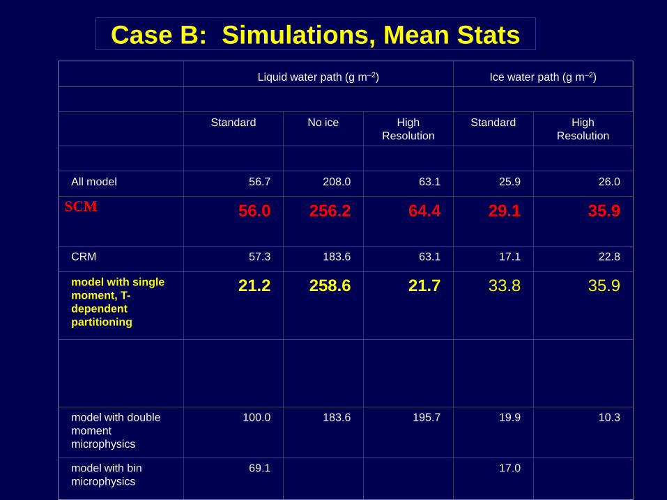
Case B: Simulations, Mean Stats

Liquid water path (g m–2) Ice water path (g m–2)

Standard No ice High

Resolution

Standard High

Resolution

All model 56.7 208.0 63.1 25.9 26.0

SCM 56.0 256.2 64.4 29.1 35.9

CRM 57.3 183.6 63.1 17.1 22.8

model with single

moment, T-

dependent

partitioning

21.2 258.6 21.7 33.8 35.9

model with double

moment

microphysics

100.0 183.6 195.7 19.9 10.3

model with bin

microphysics

69.1 17.0

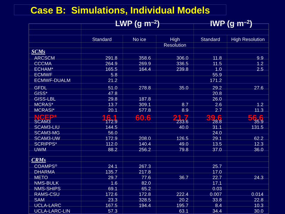
Case B: Simulations, Individual Models

LWP (g m–2) IWP (g m–2)

Standard No ice High

Resolution

Standard High Resolution

SCMs

ARCSCM 291.8 358.6 306.0 11.8 9.9

CCCMA 264.9 269.9 336.5 11.5 1.2

ECHAM* 165.5 164.4 239.8 1.0 2.5

ECMWF 5.8 55.9

ECMWF-DUALM 21.2 171.2

GFDL 51.0 278.8 35.0 29.2 27.6

GISS* 47.8 20.8

GISS-LBL 29.8 187.8 26.0

MCRAS* 13.7 309.1 8.7 2.6 1.2

MCRASI* 20.1 577.8 8.9 2.7 11.3

NCEP* 16.1 60.6 21.7 39.6 56.6SCAM3 172.9 233.6 28.8 35.9

SCAM3-LIU 144.5 40.0 31.1 131.5

SCAM3-MG 56.0 24.0

SCAM3-UW 172.9 208.0 126.5 29.1 62.2

SCRIPPS* 112.0 140.4 49.0 13.5 12.3

UWM 88.2 256.2 79.8 37.0 36.0

CRMs

COAMPS® 24.1 267.3 25.7

DHARMA 135.7 217.8 17.0

METO 29.7 77.6 36.7 22.7 24.3

NMS-BULK 1.6 82.0 17.1

NMS-SHIPS 69.1 65.2 0.03

RAMS-CSU 172.6 172.8 222.4 0.007 0.014

SAM 23.3 328.5 20.2 33.8 22.8

UCLA-LARC 167.5 194.4 195.7 8.4 10.3

UCLA-LARC-LIN 57.3 63.1 34.4 30.0

Case B: Summary

• Observation: a well-mixed boundary layer with

a cloud top temperature of –15 oC, dominant by

water cloud.

• All Models: generally underestimated LWP;

mean IWP is close to the observed.

• NCEP GFS-SCM: compared to other models,

GFS tends to have even lower LWP; GFS IWP

is more realistic.

Negative Water Vapor in the GFS

Causes Importance Solutions

Vertical Advection 1. Semi-Lagrangian

2. Flux-Limited Positive-

Definite Scheme for

current Eulerian GFS

GSI Analysis Tuning factqmin and

factqmax

Spectral Transform 1. Semi-Lagrangian GFS:

running tracers on grid, no

spectral transform

2. Eulerian GFS: no

solution yet.

Cloud Water Borrowing Limiting the borrowing to

available amount of water

vapor

SAS Mass-Flux Remains to be resolved