Engine Speed Based Estimation of the Indicated Engine … · Engine Speed Based Estimation of the...

Engine Speed Based Estimation of theIndicated Engine Torque

Master’s thesisperformed atVehicular Systems

byMagnus Hellstrom

Reg nr: LiTH-ISY-EX-3569-2005

16th February 2005

Engine Speed Based Estimation of theIndicated Engine Torque

Master’s thesis

performed atVehicular Systems,Dept. of Electrical Engineering

atLink opings universitet

by Magnus Hellstrom

Reg nr: LiTH-ISY-EX-3569-2005

Supervisor:Zandra JanssonDaimlerChrysler AG

Per AnderssonLinkopings universitet

Per ObergLinkopings universitet

Examiner: Associate Professor Lars ErikssonLinkopings universitet

Linkoping, 16th February 2005

Avdelning, InstitutionDivision, Department

DatumDate

Sprak

Language

¤ Svenska/Swedish

¤ Engelska/English

¤

RapporttypReport category

¤ Licentiatavhandling

¤ Examensarbete

¤ C-uppsats

¤ D-uppsats

¤ Ovrig rapport

¤

URL f or elektronisk version

ISBN

ISRN

Serietitel och serienummerTitle of series, numbering

ISSN

Titel

Title

ForfattareAuthor

SammanfattningAbstract

NyckelordKeywords

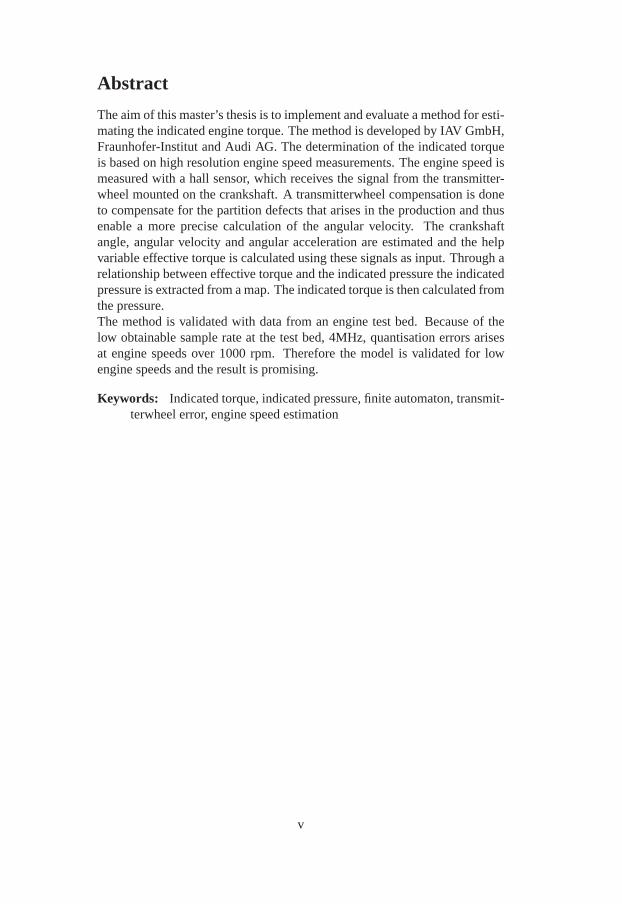
The aim of this master’s thesis is to implement and evaluate a method for es-timating the indicated engine torque. The method is developed by IAV GmbH,Fraunhofer-Institut and Audi AG. The determination of the indicated torqueis based on high resolution engine speed measurements. The engine speed ismeasured with a hall sensor, which receives the signal from the transmitter-wheel mounted on the crankshaft. A transmitterwheel compensation is done tocompensate for the partition defects that arises in the production and thus en-able a more precise calculation of the angular velocity. The crankshaft angle,angular velocity and angular acceleration are estimated and the help variable ef-fective torque is calculated using these signals as input. Through a relationshipbetween effective torque and the indicated pressure the indicated pressure is ex-tracted from a map. The indicated torque is then calculated from the pressure.

The method is validated with data from an engine test bed. Because of thelow obtainable sample rate at the test bed, 4MHz, quantisation errors arises atengine speeds over 1000 rpm. Therefore the model is validated for lowenginespeeds and the result is promising.

Vehicular Systems,Dept. of Electrical Engineering581 83 Linkoping

16th February 2005

—

LITH-ISY-EX-3569-2005

—

http://www.vehicular.isy.liu.sehttp://www.ep.liu.se/exjobb/isy/2005/3569/

Engine Speed Based Estimation of the Indicated Engine Torque

Varvtalsbaserad estimering av indikerat motormoment

Magnus Hellstrom

××

Indicated torque, indicated pressure, finite automaton, transmitterwheelerror,engine speed estimation

Abstract

The aim of this master’s thesis is to implement and evaluate amethod for esti-mating the indicated engine torque. The method is developedby IAV GmbH,Fraunhofer-Institut and Audi AG. The determination of the indicated torqueis based on high resolution engine speed measurements. The engine speed ismeasured with a hall sensor, which receives the signal from the transmitter-wheel mounted on the crankshaft. A transmitterwheel compensation is doneto compensate for the partition defects that arises in the production and thusenable a more precise calculation of the angular velocity. The crankshaftangle, angular velocity and angular acceleration are estimated and the helpvariable effective torque is calculated using these signals as input. Through arelationship between effective torque and the indicated pressure the indicatedpressure is extracted from a map. The indicated torque is then calculated fromthe pressure.The method is validated with data from an engine test bed. Because of thelow obtainable sample rate at the test bed, 4MHz, quantisation errors arisesat engine speeds over 1000 rpm. Therefore the model is validated for lowengine speeds and the result is promising.

Keywords: Indicated torque, indicated pressure, finite automaton, transmit-terwheel error, engine speed estimation

v

Thesis Outline

Outline of the master’s thesis.

Chapter 1 Introduction: A short introduction to the problem in objective.

Chapter 2 System Description:The parts of the engine that are of concernin this thesis are presented. A brief introduction to how a 4-stroke engineworks over one cycle is given.

Chapter 3 Indicated Torque Modeling: The model approach is presented.

Chapter 4 Alternating Gas Torque Calculation: The equations for calcu-lating the gas torque for a one cylinder engine are deduced and then expandedto a six cylinder engine.

Chapter 5 Manifold Pressure Dependence:A method to compensate forthe higher gas torque which occurs for turbocharged engines.

Chapter 6 Transmitterwheel error compensation: A method to compen-sate for production errors on the transmitterwheel is presented.

Chapter 7 Cycle Duration Measurements:In this chapter different ways tomeasure and estimate the crank angle, angular velocity and angular accelera-tion, are discussed. These are the signals needed to calculate the alternatinggas torque in Chapter 4.

Chapter 8 Measurements in an Engine Test Bed and in VehicleThis chap-ter presents the measurements done to get the validation data.

Chapter 9 Validation and Results:Validation and results are presented.

Chapter 10 Conclusions: The conclusions drawn from this master thesisare presented and discussed.

Chapter 11 Future Work: What can be done to improve and develop themodel and its results are discussed.

Acknowledgment

I would like to thank everybody at the DaimlerChrysler department REI/EPfor a great time. Special thanks to Stephan Terwen for help with everythingthat has to do with Matlab/Simulink, Florian Bicheler for the engine test bedmeasurements, Christian Dengler for help with everything from the coffeemachine to explaining the hardware for future measurementsand my two

vi

supervisors at Vehicular Systems Per Andersson and PerOberg for givingme feedback on my report. Last but most I want to thank my supervisor atDaimlerChrysler Zandra Jansson for input, support, feedback and making mytime here pleasant.

vii

Contents

Abstract v

1 Introduction 11.1 Objective . . . . . . . . . . . . . . . . . . . . . . . . . . . 1

2 System Description 3

3 Indicated Torque Modeling 5

4 Alternating Gas Torque Calculation 74.1 Derivation of the Moment of Inertia . . . . . . . . . . . . . 9

4.1.1 Expansion to a Six Cylinder Engine . . . . . . . . . 144.2 Indicated Pressure to Indicated Torque . . . . . . . . . . . . 15

5 Manifold Pressure Dependence 17

6 Transmitterwheel Error Compensation 196.1 Using the Sine behaviour of the Engine Speed . . . . . . . . 216.2 Using the Opposite Phase of the Gas and Mass Torque . . . 25

7 Cycle Duration Measurements 277.1 Adjustments for the Edge Signal Gap . . . . . . . . . . . . 277.2 Estimation of the Crankshaft Angle and Speed . . . . . . . . 28

7.2.1 Estimation with Constant Angular Acceleration . . . 287.2.2 Estimation with Constant Angular Velocity . . . . . 297.2.3 Estimation Every Six Degrees . . . . . . . . . . . . 29

7.3 The Estimation Algoritm Based on Finite Automaton Theory 307.3.1 Angle Synchron Engine Speed Survey . . . . . . . . 307.3.2 Forgetting factor . . . . . . . . . . . . . . . . . . . 31

8 Measurements in an Engine Test Bed and in Vehicle 328.1 Map construction . . . . . . . . . . . . . . . . . . . . . . . 34

ix

9 Validation and Results 369.1 Comparison of the Different Angle Estimation Approaches . 369.2 Transmitterwheel Error Compensation Methods . . . . . . . 38

9.2.1 The Sine Behavior of the Engine Speed . . . . . . . 389.2.2 The Opposite Phase Of The Gas And Mass Torque . 389.2.3 Summary of Transmitterwheel Compensation Methods 40

9.3 Validation of the Torque Estimation Model . . . . . . . . . . 409.3.1 Updates only Every Six Degrees . . . . . . . . . . . 409.3.2 Constant Angular Velocity between the Edges . . . . 40

10 Conclusions 42

11 Future Work 43

References 44

Notation 45

x

Chapter 1

Introduction

The engine torque signal is a very important signal for powertrain control.The torque is nowadays calculated in the control unit of the vehicles, but thecalculation does not always give an accurate result and a precise engine torquesignal is desirable. If a more precise engine torque signal could be generatedthe car could be driven closer to optimum, with lower fuel consumption andbetter comfort as merits. The best way to achieve such a precise signal wouldof course be to measure the torque and thereby getting an accurate estimate.However, due to cost and integration complexity it is not profitable to usetorque sensors in series production. Since an engine torquesensor is not anoption, new models for torque estimation are developed and tested. The en-gine torque is affected by a lot of different sources such as fuel injection, airquantity, oil temperature, the temperature of the gear oil and so on. It is im-possible to consider all interacting sources when buildinga model, so therewill always be a difference between model and reality which can lead to de-viations between the torque the engine provides and the estimated one.

Unlike torque sensors, the existing engine speed sensors are relatively cheapand accurate and it would be sensible to somehow use this information in-stead. The main topic of this master’s thesis is the implementation and testingof the accuracy and feasibility of a new engine torque model,developed byIAV GmbH, Frauenhofer-Institut and Audi AG, which uses the signal fromthe engine speed sensor as input. The model is based on the determination ofthe crankshaft position which is used for estimation of the indicated pressure.The indicated torque is then calculated from the pressure.

1.1 Objective

The objectiv of this master thesis is to implement and evaluate a method toestimate the indicated engine torque developed by IAV GmbH,Frauenhofer-

1

2 Chapter 1. Introduction

Institut and Audi AG. The method is implemented as a model in Matlab/Simulink,with compensation for the transmitterwheel error. The model is to be testedand validated with data from an engine test bed.

Chapter 2

System Description

In this master’s thesis a map based model which uses the engine speed signalas input to estimate the indicated torque is investigated. The indicated torqueis the torque generated in the cylinders and acting on the crankshaft withoutfriction.

This section gives an overview of the engine system producing the torque.The engine system considered here consists of a hall sensor,the crank shaft,a transmitterwheel, pistons and piston rods, as seen in Figure 2.1.

Piston

Piston rod

Engine speed

F

Piston rod

Piston rodPiston

Piston

X

Y Y

Z

Transmitterwheel

HALL sensor

Crankshaft

Crankshaft

Figure 2.1: The engine system, seen from two angles of perspective

3

4 Chapter 2. System Description

The engine operates in four strokes. In the first air is inhaled as the pistonmoves down, in the second the air is compressed as the piston moves up. Atthe peak of compression the fuel is injected and ignited. Theignition sets en-ergy free and increases the gas pressure in the cylinder thatforces the pistonto move down. Every time when the engine ignites there is a peak in the en-gine speed, if it is a six cylinder engine there are six peaks in the engine speedper two revolutions. The forth stroke is when the piston moves up and ejectsthe exhausts. The work delivered to the piston over the entire four strokecycle, per unit displaced volume, is called the net mean effective indicatedpressure (imep). It is an efficiency norm that can be used to compare engineswith different cylinder volumes, see [2]. The force that works on the pistonis transmitted to the crankshaft through the piston rod. Thecrankshaft is putinto rotation by the applied force and the torque on the powertrain is used toput the wheels in motion.

A combustion cycle consists of two crankshaft revolutions.A sensors on thecamshaft is used to decide if it is the first or second revolution. To be ableto tell in which part of the cycle the engine is at the moment the crankshaftposition must be known. A transmitterwheel with 60 minus 2 teeth, wherethe two teeth left out are for synchronization, is assembledon the crankshaftto enable position determination. A hall sensor receives the signal from thetransmitter wheel. The signal is used to detect when a new tooth occurs atthe hall sensor, which is equal to an edge in the hall sensor output. Everyedge implies an increase of six degrees except the one after the two teeth gapwhich implies a 18 degree change.

With the edges detected and hence the position determined, theimep can befound through estimations, calculations and maps.

Chapter 3

Indicated Torque Modeling

The model approach is presented in this chapter. The basic principle is anaccurate determination of the angular velocity and the crank shaft position.The model approach is summarized in Figure 3.1,p

boostis the boost pressure.

Figure 3.1: Model approach

Input to the model is the engine speed and output is the indicated pressureimep. The engine speed signal is recieved with a hall sensor from atransmit-terwheel seen in Figure (3.2).

S

N

1 2 3

456

1. Sensor body

2. Permanent magnet

3. Faster

4. Signal processing

5. HALL-element

6. Transmitterwheel

Figure 3.2: Hall sensor

5

6 Chapter 3. Indicated Torque Modeling

After processing the transmitterwheel signal a compensation for productionerrors on the transmitterwheel must be done (Figure 3.1 ’TransmitterwheelCompensation’). The error can be up to 0.5 degrees per tooth and the re-sult is useless without compensation of the errors. From thecompensatedtransmitterwheel signal the angle velocity is estimated via a finite automatonalgorithm, see Chapter 7.3, and the angular acceleration iscalculated throughdifferentiation of the velocity (Figure 3.1 ’Cycle Duration Measurement’).The angle is estimated between the edges from the angular velocity. Thetransmitterwheel compensation block is executed parallelto the cycle dura-tion measurement until enough data are collected to calculate the correctionfactors and perform the compensation. The estimated signals are filtered to re-duce noise interference (Figure 3.1 ’Filtering’) and the alternating gas torqueis calculated, see Chapter 4 (Figure 3.1 ’Gas Torque Calculation’). The datahave been filtered off-line with a averaging filter and different filter technicsare not investigated in this thesis. If the engine has a turbocharger a manifoldpressure compensation is done (Figure 3.1 ’Manifold Pressure Compensa-tion’) before the indicated pressure can be extracted from maps. Finally theindicated torque can be obtained from the indicated pressure.

Chapter 4

Alternating Gas TorqueCalculation

This chapter deals with the alternating gas torque block in Figure (3.1). Thealternating gas torque is the gas torque without its the meanvalue, in anal-ogy with a current without its DC part. Here the equations needed to calculatethe indicated engine torque from the engine speed are deduced and explained.

The base for the alternating gas torque is the torque balanceat the crankshaftas seen in Equation (4.1) whereTg is the gas torque,Tmass is the torque orig-inated from the oscillating and rotating masses,T

lis the load torque andTf

is torque loss due to friction. Assumptions are made for a rigid crankshaftand a sufficiently decoupled power train. This means that allinfluence on thepower train coming from the vehicles mass and gearbox is seenas a torqueincluded in the load torque.

Tg − Tmass − Tl − Tf = 0 (4.1)

The gas torque,Tg, can be split in one alternating and one direct part, wherethe direct part is the mean value.

Tg = Tg + Tg (4.2)

For the method, developed by IAV GmbH, Frauenhofer-Institut and Audi AGwhich is investigated here, conclusions of the indicated pressure are drawnfrom the alternating gas torque, see [6]. The stationary case with the directgas torque, the friction torque and the load torque in balance leads to

Tmass = Tg (4.3)

It has also been shown through tests that assuming stationarity is a good ap-proximation over a combustion cycle during transient behaviour, see [6], thatmeans that

7

8 Chapter 4. Alternating Gas Torque Calculation

Tg >> Tg − Tf − Tl (4.4)

and hence it is possible to draw conclusions of the total engine torque fromTg even in the transient case. The mass torque can be calculatedfrom thekinetic energy of the masses in motion. The kinetic energy can be expressedas:

Emass =

∫

2π

0

Tmassdϕ =1

2Θϕ2 (4.5)

which through differentiation with respect to the crankshaft angle becomesthe mass torque withϕ as the angular acceleration,ϕ as the angular velocity,Θ as the mass moment of inertia andΘ′ as the derivative of the mass momentof inertia with respect to the crank shaft angle.

Tmass =dEmass

dϕ= Θϕ +

1

2Θ′ϕ2 (4.6)

From Equation (4.3) and (4.6) an expression forTg, dependent of the enginespeed, can be obtained.

Θϕ +1

2Θ′ϕ2 ≈ Tg (4.7)

Θϕ represents the torque from the rotating masses and1

2Θ′ϕ2 represents the

torque from the oscillating masses, see [3]. The piston performs only an os-cillating movement, the crankshaft only a rotational movement and the pistonrod both an oscillating and a rotating movement. It has been shown throughtests that the integration of the alternating gas torque over a combustion cycleis proportional to the energy transformation and hence toimep [6]. Throughintegration of the mass torque over a combustion cycle withϕ0=720◦ the helpvariable effective net torque,Teff , is calculated from Equation (4.8). The ef-fective netto torque is assumed proportional to the energy transformation andhence proportional toimep.

Teff =

√

1

ϕ0

∫ ϕ0

0

(Θϕ +1

2Θ′ϕ2)dϕ ≈

√

1

ϕ0

∫ ϕ0

0

Tgdϕ (4.8)

This relationship is used to create a map where measured values of the meanengine speed,n, and calculated values of the effective net torque are assignedto measured values of the load torque.

Tload = f(Teff , n) (4.9)

The extracted load torque is used together with the calculated mean enginespeed as input to a second map where the indicated pressure isextracted.

imep = f(Tload, n) (4.10)

4.1. Derivation of the Moment of Inertia 9

From indicated pressure it is possible to calculate the indicated torque.

The two signals needed to get the indicated pressure are the engine speed,which can be measured, and the effective torque that is calculated from Equa-tion (4.8). To calculate the effective torque the moment of inertia must beknown.

4.1 Derivation of the Moment of Inertia

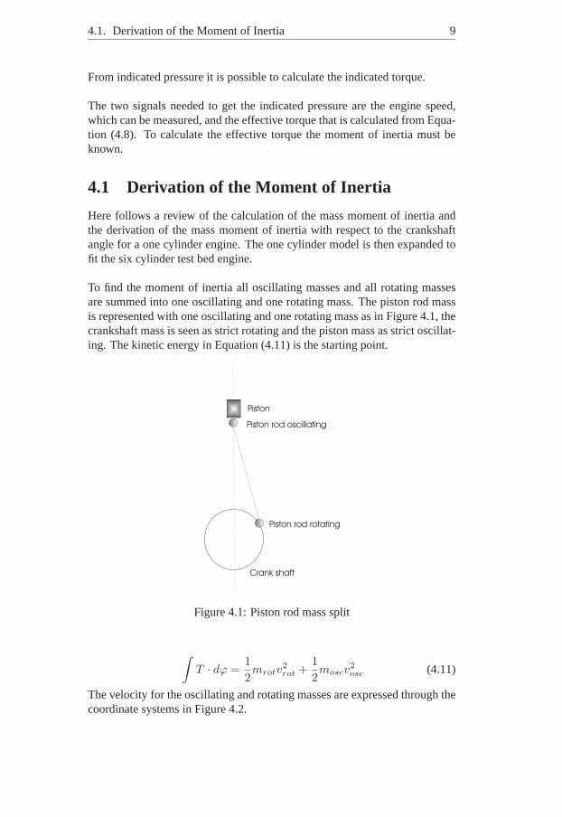
Here follows a review of the calculation of the mass moment ofinertia andthe derivation of the mass moment of inertia with respect to the crankshaftangle for a one cylinder engine. The one cylinder model is then expanded tofit the six cylinder test bed engine.

To find the moment of inertia all oscillating masses and all rotating massesare summed into one oscillating and one rotating mass. The piston rod massis represented with one oscillating and one rotating mass asin Figure 4.1, thecrankshaft mass is seen as strict rotating and the piston mass as strict oscillat-ing. The kinetic energy in Equation (4.11) is the starting point.

Crank shaft

Piston rod oscillating

Piston rod rotating

Piston

Figure 4.1: Piston rod mass split

∫

T · dϕ =1

2mrotv

2

rot +1

2moscv

2

osc (4.11)

The velocity for the oscillating and rotating masses are expressed through thecoordinate systems in Figure 4.2.


b

j

d

zrot

yrot

yosc

zosc

Figure 4.2: Coordinates to describe the mass effect on the piston rod

v2

rot = z2

rot + y2

rot (4.12)

v2

osc = z2

osc + y2

osc (4.13)

zrot = r(1 − cos ϕ) (4.14)

zrot = r sin ϕϕ (4.15)

zrot = r(sin ϕϕ + cos ϕϕ2) (4.16)

yrot = r sin ϕ (4.17)

yrot = r cos ϕϕ (4.18)


yrot = r(cos ϕϕ − sinϕϕ2) (4.19)

x is defined as the piston distance ratio,x = sr

wheres is the piston distancemeasured from the top dead center andr is as in Figure 4.5.x′ = dx

dϕis the

piston velocity ratio, andx′′ = d2xdϕ2 piston acceleration ratio.

zosc = rx (4.20)

zosc = rx′ϕ (4.21)

zosc = r(x′ϕ + x′′ϕ2) (4.22)

yosc = 0 (4.23)

Differentiation of Equation (4.11) with respect to the timeleads to Equation(4.24).

T ϕ = mrotvrotvrot + moscvoscvosc (4.24)

The velocity for the rotating and oscillating masses can be written as Equation(4.25) and (4.26).

vosc = zosc ⇒ vosc = zosc (4.25)

vrot =√

z2rot + y2

rot ⇒ vrot =zrotzrot + yrotyrot

√

z2rot + y2

rot

(4.26)

Equation (4.25) and (4.26) in (4.24) leads to the expressionbelow.

T ϕ = mrot(zrotzrot + yrotyrot) + mosczosczosc (4.27)

With Equation (4.15), (4.16), (4.18), (4.19), (4.21), (4.22) in Equation (4.27)

T = ϕ(r2mrot + moscr2x′2) + ϕ2(moscr

2x′x′′) (4.28)

the moment of inertia for a one cylinder engine is identified from equation(4.7)

Θ = mrotr2 + moscr

2x′2 (4.29)

and so is the derivative of the mass moment of inertia with respect to thecrankshaft angle

Θ′ =dΘ

dϕ= 2moscx

′x′′r2 (4.30)


0° 120° 240° 360° 480° 600° 720°0.0095

0.01

0.0105

0.011

0.0115

Crankshaft Angle [degrees]

Mom

ent o

f Ine

rtia

[kgm

2 ]

Figure 4.3: The moment of inertia for a one cylinder engine

0° 120° 240° 360° 480° 600° 720°−2

−1.5

−1

−0.5

0

0.5

1

1.5

2x 10

−3


Der

ivat

ion

of th

e M

omen

t of I

nert

ia [k

gm2 ]

Figure 4.4: The derivative of the moment of inertia w.r.t thecrankshaft angle

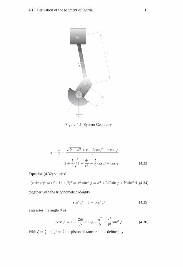
How the moment of inertia and the derivative of the moment of inertia changewith respect to the crankshaft angle can be seen in Figure 4.3and 4.4. Theengine data are taken from the test engine.The piston distance ratiox = s

rcan be rewritten through the geometrical

relations found in Figure 4.5, using Equation 4.31 and 4.32.x′ andx′′ arecalculated through differentiation ofx with respect to the crankshaft angle.Notice that a displacement,d, as in Figure 4.5 is defined as a negative dis-placement.

s =√

l2 − d2 + r − l cos β − r cos ϕ (4.31)

r sin ϕ = d + l sinβ (4.32)

This result in Equation (4.33).


l

r

d

b

j

Figure 4.5: System Geometry

x =s

r=

√l2 − d2 + r − l cos β − r cos ϕ

r

= 1 +l

r

√

1 − d2

r2− l

rcos β − cos ϕ (4.33)

Equation (4.32) squared

(r sinϕ)2 = (d + l sin β)2 ⇒ r2 sin2 ϕ = d2 + 2dl sinϕ + l2 sin2 β (4.34)

together with the trigonometric identity

sin2 β = 1 − cos2 β (4.35)

expresses the angleβ as

cos2 β = 1 +2dr

l2sin ϕ − d2

l2− r2

l2sin2 ϕ (4.36)

With ξ = rl

andµ = dl

the piston distance ratio is defined by:


x = 1 +1

ξ

√

1 − µ2 − 1

ξ

√

1 + 2ξµ sin ϕ − ξ2 sin2 ϕ − µ2 − cos ϕ (4.37)

Through one respectively two differentiations with respect to the crankshaftangle the piston velocity ratio (Equation (4.38)) and piston acceleration ratio(Equation (4.39)) are deduced.

x′ =( dx

dϕ

)

= sin ϕ +ξ sin ϕ cos ϕ − µ cos ϕ

√

1 − ξ2 sin2 ϕ + 2ξµ sin ϕ − µ2

(4.38)

x′′ = cos ϕ +ξ cos2 ϕ − ξ sin2 ϕ + ξ3 sin4 ϕ + 3ξµ2 sin2 ϕ

(√

1 − ξ2 sin2 ϕ + 2ξµ sin ϕ − µ2)3

− 3ξ2µ sin3 ϕ + µ sin ϕ − µ3 sin ϕ

(√

1 − ξ2 sin2 ϕ + 2ξµ sin ϕ − µ2)3(4.39)

With the geometry for the test engine used in this thesis the different ratios,x,x′, x′′, over a combustion cycle are visualised in Figure 4.6. Between 60-90degrees the velocity ratio has its highest values. In this range the mass forcescontributes at most to the angle velocity variations.

0° 120° 240° 360° 480° 600° 720°−1.5

−1

−0.5

0

0.5

1

1.5

2

2.5


Rat

io

DistanceVelocityAcceleration

Figure 4.6: Distance (x), velocity (x′) and acceleration (x′′) ratio

x, x′ andx′′ are used in Equation (4.29) and (4.30) to calculate the momentof inertia and the derivative of the moment of inertia.

4.1.1 Expansion to a Six Cylinder Engine

The moment of inertia deduced in the last section is for a one cylinder engine.If there are more pistons attached to the crankshaft they arealso contributing

4.2. Indicated Pressure to Indicated Torque 15

to the mass moment of inertia and their contribution change with respect tothe crankshaft angle. Because of the 120◦ shift between the piston cycles andthe assumption of a rigid crankshaft the moment of inertia for a six cylinderengine can be calculated from the moment of inertia of a one cylinder engine(Equation 4.29) shifted six times with 120◦ and then superposed. How thesix cylinder moment of inertia and its derivation change with respect to thecrankshaft angle can be seen in Figure 4.7 and 4.8.

0° 120° 240° 360° 480° 600° 720°0.061

0.0615

0.062

0.0625

0.063

0.0635

0.064


Mom

ent o

f Ine

rtia

[kgm

2 ]

Figure 4.7: The moment of inertia for the six cylinder engineM272

0° 120° 240° 360° 480° 600° 720°−4

−3

−2

−1

0

1

2

3

4x 10

−3


Der

ivat

ion

of th

e M

omen

t of I

nert

ia [k

gm2 ]

Figure 4.8: The derivative of the moment of inertia for the six cylinder engineM272

4.2 Indicated Pressure to Indicated Torque

To calculate the indicated torque from the indicated pressure one can firstcalculate the indicated power and therefrom the torque. To get the indicated


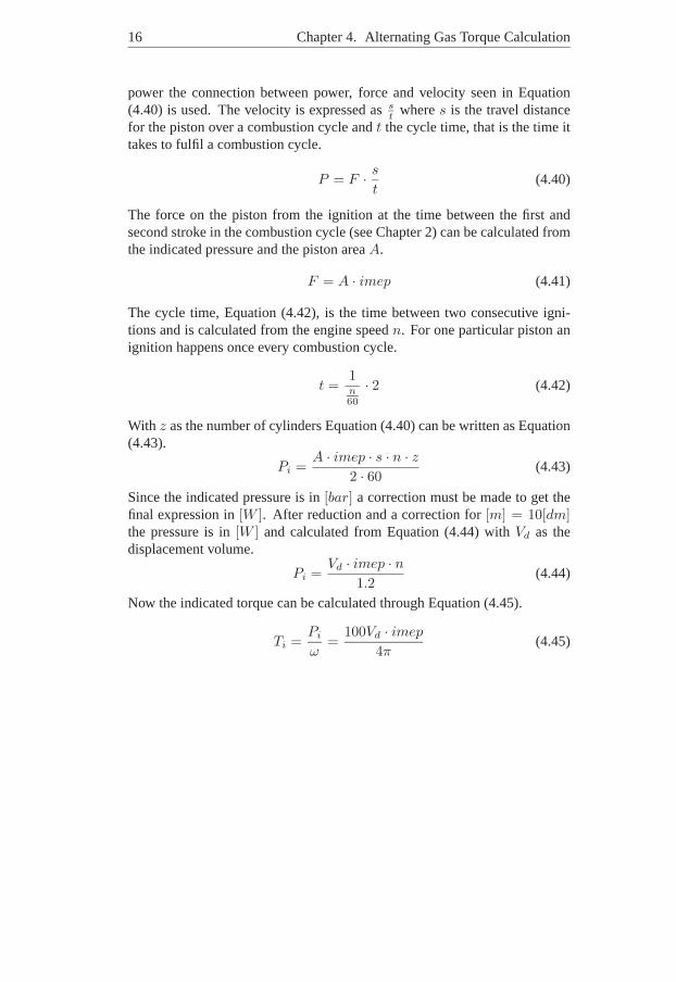
power the connection between power, force and velocity seenin Equation(4.40) is used. The velocity is expressed ass

twheres is the travel distance

for the piston over a combustion cycle andt the cycle time, that is the time ittakes to fulfil a combustion cycle.

P = F · s

t(4.40)

The force on the piston from the ignition at the time between the first andsecond stroke in the combustion cycle (see Chapter 2) can be calculated fromthe indicated pressure and the piston areaA.

F = A · imep (4.41)

The cycle time, Equation (4.42), is the time between two consecutive igni-tions and is calculated from the engine speedn. For one particular piston anignition happens once every combustion cycle.

t =1n60

· 2 (4.42)

With z as the number of cylinders Equation (4.40) can be written as Equation(4.43).

Pi =A · imep · s · n · z

2 · 60(4.43)

Since the indicated pressure is in[bar] a correction must be made to get thefinal expression in[W ]. After reduction and a correction for[m] = 10[dm]the pressure is in[W ] and calculated from Equation (4.44) withVd as thedisplacement volume.

Pi =Vd · imep · n

1.2(4.44)

Now the indicated torque can be calculated through Equation(4.45).

Ti =Pi

ω=

100Vd · imep

4π(4.45)

Chapter 5

Manifold PressureDependence

This chapter concerns the manifold pressure dependence block in Figure 3.1.The model should provide accurate information independently of it is an en-gine with turbocharger or not. A turbocharger provides a higher alternatinggas torque amplitude which could cause problems concerningthe map ex-traction. This is not considered in this thesis because the engine used for themeasurements does not have a turbocharger. If an engine withturbochargershould be investigated, the manifold pressure dependence could be normal-izied by a map that normalizes the alternating gas torque amplitude and makeit independent from manifold pressure as described in [6]. It is a linear rela-tionship (Figure 5) which also make the gas torque independent of the atmo-sphere pressure.

1

Cmax

Pmax

C

P [bar]

Figure 5.1: Linear manifold pressure dependence

17

18 Chapter 5. Manifold Pressure Dependence

The compensation factor is extracted from a map and multiplied with alter-nating gas torque, as in Equation (5.1), resulting in a compensated gas torque.The compensated gas torque is used as input for the indicatedtorque map.

Mgcompensated=

Mg

c(5.1)

Chapter 6

Transmitterwheel ErrorCompensation

In this chapter a method to compensate for the transmitterwheel error is pre-sented. The compensation is represented by the transmitterwheel error blockin Figure 3.1. One source that affects the accuracy of the angular velocity cal-culation are the teeth partition defects of the transmitterwheel that can arise inproduction, see Figure 6.1. This error is different for every tooth on the trans-mitterwheel. The error can be up to0.5◦ [7] and must be taken into accountand compensated for.

Production errors

Figure 6.1: Different width between the teeth

To be able to do this the behaviour of the the engine speed overa combustioncycle must be known. For this purpose a model built in Matlab/Simulinkis used when solving Equation 6.1 (the same equation as 4.7, but now withload and friction torque as one variable,Tlf = Tl + Tf ) numerically. Fromthe obtained angle acceleration the angle velocity is then calculated throughintegration.

ϕ =1

2

Θ′(ϕ)

Θ(ϕ)· ϕ2 − Tg(ϕ)

Θ(ϕ)− Tlf

Θ(ϕ)(6.1)

More about the model is to be read in [4]. The mass torque is modeled fromEquation (4.6) and the load and friction torque are set to zero as approxi-

19

20 Chapter 6. Transmitterwheel Error Compensation

mation of the forces from the street almost equals the friction forces over acombustion cycle during motored cycles. Therefore only data obtained dur-ing motored cycles can be used to calculate the correction factors, which arethe aim of this transmitterwheel compensation algorithm. The gas torque iscalculated from Equation 6.2 [1].

Tg = (pcyl − p0)Ap

ds

dϕ(6.2)

Ap is the piston area,pcyl is the pressure in the cylinder andp0 is the at-mosphere pressure. The cylinder pressure is crankshaft angle dependent andcalculated for one cylinder and then shifted six times 120◦ and superposed tofit a six cylinder engine [1]. WithTg andTmass known the simulink modelis used to solve Equation (6.1) which gives an approximationof the enginespeed. Below are three figures that show the engine speed during motoredcycles. Here interesting changes in the behavior of the engine speed at low,middle and high engine speed can be seen. Since no effort has been put inthe parametrisation of the engine speed model the values on the y-axis areincorrect and only the relation between the engine speeds inthe three figuresare of interest.

0° 120° 240° 360° 480° 600° 720°185

190

195

200

205

210

215


Eng

ine

Spe

ed [r

pm]

Figure 6.2: Behavior of low engine speed during motored cycles

6.1. Using the Sine behaviour of the Engine Speed 21

0° 120° 240° 360° 480° 600° 720°380

385

390

395

400

405

410

Eng

ine

Spe

ed [r

pm]


Figure 6.3: Behavior of the engine speed when the gas and massforces are inbalance

0° 120° 240° 360° 480° 600° 720°1975

1980

1985

1990

1995

2000

2005

Eng

ine

Spe

ed [r

pm]


Figure 6.4: Behavior of high engine speed during motored cycles

The mass torque and the gas torque works against each other. The oscilla-tions at low engine speeds, Figure 6.2, are caused by the gas torque. Withincreasing engine speed the mass torque contribution increase and because ofthe opposite direction from the gas torque they are in balance at a certain en-gine speed which means there are almost no oscillations, Figure 6.3. At highengine speeds the mass torque is much higher than the gas torque and causessine formed oscillations, Figure 6.4. These properties of the engine speed canbe used in different ways to compensate for the transmitter wheel error.

6.1 Using the Sine behaviour of the Engine Speed

As seen in Figure 6.4 the engine speed behaves like a sine curve at highermean engine speeds at motored cycles. This knowledge can be used to de-


termine the transmitterwheel error for every single tooth.This is done bymeasuring the angular velocity for every tooth on the transmitterwheel overa whole combustion cycle during motored cycles, see Equation (6.3), at amean engine speed high enough to produce a sine wave. The loadand fric-tion torque and the quantisation errors are not periodic andtheir effect on aspecial tooth is seen as stochastic disturbance which can bereduced throughaveraging.

ω =

ω1

ω2

...ω120

(6.3)

The time for every tooth is calculated from the angular velocity in Equation(6.4).

t = ω−1 =

t1t2...

t120

t

(6.4)

To get a measure of how constant the mean engine speed is over the combus-tion cycle, the variance for the time vector is calculated inEquation (6.5). Themore constant the engine speed is the less engine speed change correction, seeFigure 6.6, must be done.

var(t) =1

k

k∑

i=1

(t(i) − 〈t〉)2 k = 120 (6.5)

The procedure is then repeated from the beginning and the variance from thelatest time vector is always compared with the lowest variance from the ear-lier vectors. If the variance is lower, the new time vector issaved and theother is erased. Afterx combustion cycles, withx chosen properly, the meanengine speed is considered constant enough, and its corresponding time vec-tor, tteeth, is saved. To make the method more insensitive towards stochasticdisturbances like misfire in one of the cylinders, changes inthe load torqueand quantisation errors a number oftteeth are calculated and an average isgenerated as in Equation (6.6).

taverage =tteeth1

+ tteeth2+ . . . + tteethm

m(6.6)

Based on a perfect transmitterwheel, and with the assumption that the enginespeed is a sine wave during motored cycles, the frequency component of themeasured engine speed that corresponds to the perfect engine speed is de-rived via fourier series representation. Equation (6.7) represents the intended

6.1. Using the Sine behaviour of the Engine Speed 23

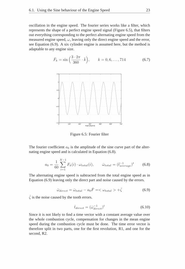
oscillation in the engine speed. The fourier series works like a filter, whichrepresents the shape of a perfect engine speed signal (Figure 6.5), that filtersout everything corresponding to the perfect alternating engine speed from themeasured engine speed,ω, leaving only the direct engine speed and the error,see Equation (6.9). A six cylinder engine is assumed here, but the method isadaptable to any engine size.

Fk = sin(3 · 2π

360· k

)

, k = 0, 6, . . . , 714 (6.7)

0° 120° 240° 360° 480° 600° 720°−1.5

−1

−0.5

0

0.5

1

1.5

Angle [degrees]

Figure 6.5: Fourier filter

The fourier coefficienta0 is the amplitude of the sine curve part of the alter-nating engine speed and is calculated in Equation (6.8).

a0 =1

60

N−1∑

i=1

Fk(i) · ωtotal(i), ωtotal = (t−1

average)t (6.8)

The alternating engine speed is subtracted from the total engine speed as inEquation (6.9) leaving only the direct part and noise causedby the errors.

ωdirect = ωtotal − a0F =< ωtotal > +ζ (6.9)

ζ is the noise caused by the tooth errors.

tdirect = (ω−1

direct)t (6.10)

Since it is not likely to find a time vector with a constant average value overthe whole combustion cycle, compensation for changes in themean enginespeed during the combustion cycle must be done. The time error vector istherefore split in two parts, one for the first revolution, R1, and one for thesecond, R2.


tdirect1 =

tdirect1

tdirect2

...tdirect60

tdirect2 =

tdirect61

tdirect62

...tdirect120

The mean engine speed difference between R2 and R1 is calculated by Equa-tion (6.11).

ωchange =60

∑

tdirect2

− 60∑

tdirect1

(6.11)

R1 R2

Mean engine speed

Mean engine speed

Mean engine speed change

Figure 6.6: Engine speed change, first and second revolution

The mean engine speed change is assumed linear over the combustion cycleas seen in Figure 6.6. Correction for the change is made for R2and the en-gine speed with errors is distributed evenly over all teeth in equation (6.12),see Figure 6.7. This gives the engine speed for every tooth onthe transmitter-wheel like it would be if there was no transmitterwheel errors.

ωcorrect = ωchange ·1

60·

12...

60

+( 60

∑

tdirect2

− 1

2ωchange

)

(6.12)

For easy correction of the measured time between two flanks, acorrectionfactor is calculated.

K =

K1

K2

...K60

= 1 − (tdirect2 − ω−1

correct)ωcorrect (6.13)

6.2. Using the Opposite Phase of the Gas and Mass Torque 25

R1 R2

Mean engine speed

Mean engine speedMean engine speed change / 2

Figure 6.7: Engine speed change, linear distributed

The correction factor is multiplied with its correspondingtime to get correcttime and engine speed measurements. If it is only 58 teeth on the ransmitter-wheel there will be only 58 correction factors.

6.2 Using the Opposite Phase of the Gas and MassTorque

Another approach for correction of transmitterwheel errors has been devel-oped by Frauenhofer-Institut fur Informations- und Datenverarbeitung (ITTB)and is described in [7]. The approach uses the opposite phaseof the gas andmass torque, see Figure 6.3, to find out the geometry defects on the trans-mitterwheel and compensate for them. First a specific enginespeed range isdefined, fromnmin to nmax, in which the gas and mass torque oscillationsare balanced in average. Then the length between two teeth are estimated bymultiply the measured time,tn= 1

fn, with the estimated angular velocity,ωn.

The angular velocity is estimated as the mean engine speed.

ϕnerror(z) = tn(z) · ωn =

ωn

fn(z)(6.14)

Hereϕnerroris the length of gapz with the error,z is the tooth gap index and

fn(z) is the measure frequency for this gap.To get the relative error,δerror(z), for a gapz the estimated incrementallength is subtracted with the ideal incremental length,ϕz, and a mean averageover the upper and lower engine speed bound is calculated to even the effectsfrom the gas and mass torque.


δerror =1

nmax − nmin

nmax∑

n=nmin

[ωn

fn

− ϕz

]

(6.15)

K = 1 + δerror

30

π(6.16)

In this approach it is assumed that the gas and mass torque arein perfectbalance over a specific engine speed range. One advantage with this approachis the low complexity and that it is parameter independent.

Chapter 7

Cycle DurationMeasurements

The cycle duration measurement block in Figure 3.1 is the part of the modelwhere the angle, angular velocity and angular accelerationare measured andestimated from the hall signal and which are then used in the block ’alternat-ing gas torque’ for calculations (see Chapter 4).

7.1 Adjustments for the Edge Signal Gap

The output from the hall sensor is a signal with an edge for every occuringtooth. To handle the abnormality of the two teeth gap in this edge signal, seeFigure 7.1, the torque calculations must be delayed at least18 degrees so thefirst tooth on the new revolution occurs after the gap before new calculationscan be done.

}

T

58 1

Figure 7.1: Signal with 58 teeth

27

28 Chapter 7. Cycle Duration Measurements

7.2 Estimation of the Crankshaft Angle and Speed

To get a sufficiently good estimation of the angle, angle velocity and angleacceleration in, three different approaches are considered. Two of them arebased on assumptions about the velocity and acceleration between two posi-tive edges. In the first approach constant acceleration is assumed so that theangle and angular velocity are recalculated at every sampletime. The secondapproach assumes constant angular velocity and only the angle is recalcu-lated at every sample time. The third approach makes use of the first twoapproaches, but makes an update of angle, angle speed and angle accelerationonly every six degrees.

7.2.1 Estimation with Constant Angular Acceleration

For the first approach the angle acceleration,α, is estimated from the angularvelocity at edgei andi − 1, as in Equation (7.1) where∆t = ti − ti−1.

αi =ωi − ωi−1

∆t(7.1)

The angular acceleration is then assumed constant to the next edgei + 1,see Figure 7.2. Now the angular velocity between edgei and i + 1 can beestimated at every samplen wheren is the reference signal in Figure 7.5.

ω(n) = ω(n − 1) + αi · tsamp (7.2)

The angle is calculated with the estimated velocity.

ϕ(n) = ϕ(n − 1) + (ω(n) − ω(n − 1)) · tsamp (7.3)

{{ {

} }

w1 w2 w3

a1 a2 a3

j1 j2 j3

w = wn-1+ a1tsamp w = wn-1+ a2tsamp

j = jn-1+( wn-wn-1) tsamp j = jn-1+( wn-wn-1) tsamp

Figure 7.2: Constant angular acceleration between the edges

7.2. Estimation of the Crankshaft Angle and Speed 29

7.2.2 Estimation with Constant Angular Velocity

For the second approach the calculated velocity at edgei is considered con-stant until edgei + 1. Then the angle can be estimated from Equation (7.4)using a counter which counts the number of samples between edgei andi+1(Figure 7.3).

ϕ(n) = ϕ(i) + ω(i) · counter · tsamp (7.4)

{{ {

} }

w1 w2 w3

a1 a2 a3

j1 j2 j3

j = j1+ w1tsamp counter j = j2+ w2tsamp counter

Figure 7.3: Constant angular velocity between the edges

7.2.3 Estimation Every Six Degrees

Tests are also done with a third method with updates and calculations onlyevery positive edge, i.e every six degrees whereas the methods described in7.2.1 and 7.2.2 interpolates between the edges. This means that no calcula-tions are made between the edges, less calculation means higher model speedbut the angle resolution is not better than six degrees, see Figure 7.4. Thismethod is especially interesting since it enables the evaluation of the trade offbetween loss of accuracy and gain in model calculation time.

{{ {w1 w2 w3

a1 a2 a3

j1 j2 j3

Figure 7.4: Updates only at a positive edge

30 Chapter 7. Cycle Duration Measurements

7.3 The Estimation Algoritm Based on Finite Au-tomaton Theory

The estimation algorithm used to calculate the angular velocity at every newedge from the transmitterwheel signal is based on finite automaton theory. Itis explained in this section.

The crankshaft angle can be measured only every six degrees,i.e when apositiv edge on the transmitterwheel occurs. The estimation algorithm usesthe last calculated angular velocity to decide the positionof the crank shaft.The angular velocity is calculated, when a positive edge appears, using thisdifferential equation:

ω =∆ϕ

∆t(7.5)

There are two different approaches of the finite automaton, time synchron andangle synchron. Only the angle synchron engine speed surveyis discussedhere because of better results in [5].

7.3.1 Angle Synchron Engine Speed Survey

The time interval over an increment angle, e.g∆ϕ = 6◦, is measured withthe help of an internal clock that counts the number of samples between twoconsecutive positive edges.

∆t = counter · tref · K, tref = tsamp (7.6)

7.3. The Estimation Algoritm Based on Finite Automaton Theory 31

K is the transmitterwheel error correction factor that is derived in Chapter 6.

Figure 7.5: Time measurement between two edges

In Figure 7.5 one can see that the accuracy increases with shorter sample time.This also means that the algorithm has a lower accuracy at a higher enginespeed because of the decreased time between two flanks.

7.3.2 Forgetting factor

To make the angular velocity and the angular acceleration estimation lessnoise sensitive a forgetting factork is used to include information from theformer measurements into the new one.

ωik= kωi + (1 − k)ωi−1 (7.7)

The biggerk is the more trust is put in the new measurement. If the signalis interfered by noise this could result in large deviationsbetween the newcalculated angular velocity and its real value. With a smaller k value, lesstrust is put in the new measurement, would mitigate the impact of the errorbut make the system dynamic slower. The determination ofk is a compromisebetween system response time and noise sensitivity and it was chosen to k=0.7through trial and error.

Chapter 8

Measurements in an EngineTest Bed and in Vehicle

To get data for the map construction discussed in Chapter 4, and to modelvalidation, measurements was made in an engine test bed. Thedata is split upin two parts. One for map constuction and the other one for model validation.The engine speed was measured with an optical sensor every crank angle de-gree. The indicated pressure,imep, was measured with a sensor at differentcombinations of load torque and engine speed.

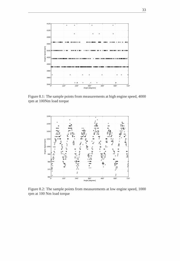
The conditions at the test bed were not good enough to give accurate measure-ments over the whole engine speed spectrum. At the test bed the maximumsample rate, the reference signal in Figure 7.5, was 4MHz. Thus quantisa-tion errors influenced the measurements for higher engine speeds, as seenin Figure 8.1. A sample rate of 4MHz means a new edge in the referencesignal everytref = 1

4MHz= 2.5 · 10−7s. If the engine speed isn =

4000rpm = 24000 degrees/s it takestcrank = 1/24000 = 4.17 ·10−5s. forthe crankshaft to rotate one degree. Under these conditionsthe quantisationsteps are in the range oftref

tcrank· n = 0.006 · 4000 = 24rpm which corre-

spond to the quantisation steps in Figure 8.1. For lower engine speeds thiseffect was not as pronounced (Figure 8.2), enabling a satisfactory measuringof the dynamic engine speed. These results, for the lower engine speeds, wereused for model validation. As the transmitterwheel compensation needs thetransmitterwheel signal with a six degrees resolution for validation, transmit-terwheel measurements were made in a test vehicle in addition to the enginetest bed measurements.

32

33

0° 120° 240° 360° 480° 600° 720°3940

3960

3980

4000

4020

4040

4060

4080

4100

4120

Eng

ine

Spe

ed [r

pm]

Angle [degrees]

Figure 8.1: The sample points from measurements at high engine speed, 4000rpm at 100Nm load torque

0° 120° 240° 360° 480° 600° 720°960

970

980

990

1000

1010

1020

1030

1040

Eng

ine

Spe

ed [r

pm]

Angle [degrees]

Figure 8.2: The sample points from measurements at low engine speed, 1000rpm at 100 Nm load torque

34 Chapter 8. Measurements in an Engine Test Bed and in Vehicle

8.1 Map construction

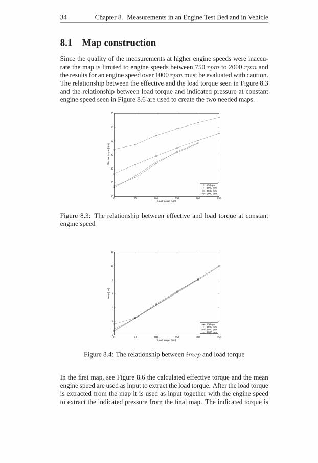
Since the quality of the measurements at higher engine speeds were inaccu-rate the map is limited to engine speeds between 750rpm to 2000rpm andthe results for an engine speed over 1000rpm must be evaluated with caution.The relationship between the effective and the load torque seen in Figure 8.3and the relationship between load torque and indicated pressure at constantengine speed seen in Figure 8.6 are used to create the two needed maps.

0 50 100 150 200 25010

20

30

40

50

60

70

Load torque [Nm]

Effe

ctiv

e to

rque

[Nm

]

750 rpm1000 rpm1500 rpm2000 rpm

Figure 8.3: The relationship between effective and load torque at constantengine speed

0 50 100 150 200 2500

2

4

6

8

10

12

Load torque [Nm]

imep

[bar

]

750 rpm1000 rpm1500 rpm2000 rpm

Figure 8.4: The relationship betweenimep and load torque

In the first map, see Figure 8.6 the calculated effective torque and the meanengine speed are used as input to extract the load torque. After the load torqueis extracted from the map it is used as input together with theengine speedto extract the indicated pressure from the final map. The indicated torque is

8.1. Map construction 35

then calculated from Equation (4.45).

600800

10001200

14001600

18002000

0

50

100

150

200

25010

20

30

40

50

60

70

Engine speed [rpm]Load torque [Nm]

Effe

ctiv

e to

rque

[Nm

]

Figure 8.5: Map to extract the load torque

600800

10001200

14001600

18002000

0

50

100

150

200

2500

2

4

6

8

10

12

Engine speed [rpm]Load torque [Nm]

imep

[bar

]

Figure 8.6: Map to extract theimep

Chapter 9

Validation and Results

The validation and results of the different estimation approaches, transmitter-wheel error compensation and the complete model are presented.

9.1 Comparison of the Different Angle Estima-tion Approaches

For the validation of the different approaches for estimating the angular ve-locity, presented in Chapter 7 an engine model is used. The model has thesame parameters as the engine test bed and delivers a processed hall sensorsignal with an edge for every tooth.

The first attempt to estimate the angle and angular velocity,as described inSection 7.2.1 did not give the desired results when validated. As seen in Fig-ure 9.1 the angular velocity becomes noisy and through the velocity updatesin between the edges errors arise at every transmitterwheelgap. The influ-ence of the gap is seen in the second and the fifth peak in the figure. Anotherdisadvantage is that the interpolation calculations in between the edges makesthe approach more complex which would make it hard to realizeit on-line.The estimation approach to update the calculations only at every edge, as de-scribed in section 7.2.3, gives accurate results for the 58 edges signal withinterpolation in the gap, as can be seen in figure 9.2. To update only at everyedge demands much less calculations compared with the approaches using in-terpolation in between the edges and is therefore the approach to use if thereare on-line demands.

36

9.1. Comparison of the Different Angle Estimation Approaches 37

0.2 0.21 0.22 0.23 0.24 0.25265

270

275

280

Time [s]

Ang

ular

vel

ocity

[rad

/s]

The original edge signal is used with estimation

as desribed in Section 7.2.1

Desired angular velocityEstimated angular velocity

Figure 9.1: The estimated signal is noisy and in the second and fifth peak theinfluence of the two teeth gap is seen

0.2 0.21 0.22 0.23 0.24 0.25265

270

275

280

Time [s]

Ang

ular

vel

ocity

[rad

/s]

The original edge signal is used with estimation

as in Section 7.2.2

Desired angular velocityEstimated angular velocity

Figure 9.2: The estimated signal fits the desired signal well. In the secondand fifth peak the influence of the two teeth gap is smaller thenin Figure 9.1

The estimation of the angle with constant angular velocity between the edges,discussed in Section 7.2.2, estimates the angular velocityonly at every edge.This approach includes however interpolation of the angle in between theedges and is therefore not suited for on-line use.

38 Chapter 9. Validation and Results

The conclusions drawn from the validation with the engine model are that theestimation of the angle with constant angular velocity between the edges andthe estimation with updates only at every edge with interpolation in the gapare of further interest. The other methods can be discarded.

9.2 Transmitterwheel Error Compensation Meth-ods

To make the validation of the transmitterwheel error compensation possiblea special developed hardware which enables20MHz resolution was used.The engine speed was measured over an inductive sensor in a test vehicle asmentioned in Chapter 8. The measurements were used to validate the trans-mitterwheel error compensation but not to validate the whole model becausethe indicated pressure and the load torque could not be measured in the testcar.

9.2.1 The Sine Behavior of the Engine Speed

The method validated is presented in Section 6.1. To calculate the correctionfactors a measurement during motored cycles with the enginespeed droppingfrom 5000 to 1400 rpm was used. As seen in Figure 9.3 the result is notsatisfactory. The six combustion variations that ought to be seen over a com-bustion cycle after compensation are not visible. The reason why the methoddoes not work properly is that the assumption, that the oscillation in the en-gine speed is a sine curve at high mean engine speed during motored cycles,is false. It means that there are oscillations left in the engine speed whenthe correction factors are calculated which leads to errorsin the correctionfactors.

9.2.2 The Opposite Phase Of The Gas And Mass Torque

The method using the opposite phase of the gas and mass torqueis describedin Section 6.1. The correction factors was calculated from engine speed in-creased from1400 to 3500 rpm. The boundary for the engine speed in whichthe gas and mass torque were in balance were found through trial and errorand thus chosen tonmin = 1700 andnmax = 2300. The result seen in Figure9.4 is satisfactory and it is possible to detect all six combustion in the enginespeed signal. The peaks seen in the signal without compensation says nothingabout the combustions and originates from the errors.

9.2. Transmitterwheel Error Compensation Methods 39

3.413 3.4135 3.414 3.4145 3.415 3.4155 3.416 3.4165 3.417 3.4175 3.418

x 104

2055

2060

2065

2070

2075

2080

2085

2090

2095

Time [s]

Eng

ine

spee

d [r

pm]

With compensationWithout compensation

Figure 9.3: Engine speed over a combustion cycle before and after transmit-terwheel error compensation.

2.849 2.8495 2.85 2.8505 2.851 2.8515 2.852 2.8525 2.853 2.8535 2.854

x 104

1955

1960

1965

1970

1975

1980

1985

1990

1995

2000

Time [s]

Eng

ine

spee

d [r

pm]

With compensationWithout compensation

Figure 9.4: Engine speed over a combustion cycle before and after transmit-terwheel error compensation.

40 Chapter 9. Validation and Results

9.2.3 Summary of Transmitterwheel Compensation Meth-ods

The method validated in Section 9.2.2 gives satisfying results and is thus usedto generate a satisfying input signal to the complete torqueestimation modelwhich will be validated in Section 9.3. To validate the transmitterwheel errorcompensation the signal from the transmitterwheel is needed as input. Thissignal was as mentioned in Section 9.2 measured with an inductive sensor ina test vehicle and is measured in the same way in serie produced cars.

9.3 Validation of the Torque Estimation Model

To validate the model with a six degree signal every six sample from the onedegree resolution signal measured in the engine test bed, see Chapter 8, wereused. The data used for validation is taken from the remaningpart not usedwhen creating the maps.

9.3.1 Updates only Every Six Degrees

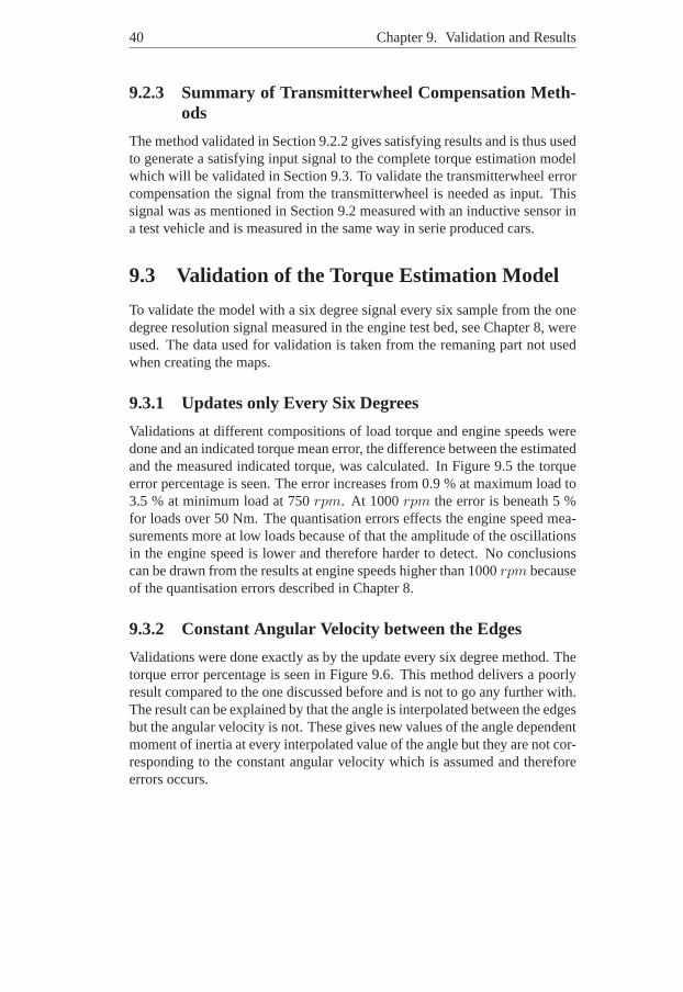
Validations at different compositions of load torque and engine speeds weredone and an indicated torque mean error, the difference between the estimatedand the measured indicated torque, was calculated. In Figure 9.5 the torqueerror percentage is seen. The error increases from 0.9 % at maximum load to3.5 % at minimum load at 750rpm. At 1000rpm the error is beneath 5 %for loads over 50 Nm. The quantisation errors effects the engine speed mea-surements more at low loads because of that the amplitude of the oscillationsin the engine speed is lower and therefore harder to detect. No conclusionscan be drawn from the results at engine speeds higher than 1000 rpm becauseof the quantisation errors described in Chapter 8.

9.3.2 Constant Angular Velocity between the Edges

Validations were done exactly as by the update every six degree method. Thetorque error percentage is seen in Figure 9.6. This method delivers a poorlyresult compared to the one discussed before and is not to go any further with.The result can be explained by that the angle is interpolatedbetween the edgesbut the angular velocity is not. These gives new values of theangle dependentmoment of inertia at every interpolated value of the angle but they are not cor-responding to the constant angular velocity which is assumed and thereforeerrors occurs.

9.3. Validation of the Torque Estimation Model 41

0

10

20

30

40

50

60

70

80

90

100

750

rpm

1000

rpm

1500

rpm

2000

rpm

0 Nm load torque

50 Nm load

torque

100 Nm load

torque

150 Nm load

torque

200 Nm load

torque

%

Figure 9.5: The indicated torque error percentage

0

50

100

150

200

250

300

350

400

450

500

750

rpm

1000

rpm

1500

rpm

2000

rpm

0 Nm load torque

50 Nm load

torque

100 Nm load

torque

150 Nm load

torque

200 Nm load

torque

%

Figure 9.6: The indicated torque error percentage

Chapter 10

Conclusions

The aim of this master thesis was to implement and evaluate a method toestimate the indicated engine torque developed by IAV GmbH,Fraunhofer-Institut and Audi AG. Measurements on an engine test bed was made to con-struct the needed maps and to get data for validation of the torque estimationmodel. Measurements in a test vehicle was made to get data forvalidation ofthe transmitterwheel error compensation method. The method is based uponengine speed measurements with a resolution high enough to catch the dy-namic behavior of the engine speed. With the measurements from the testvehicle the transmitterwheel error compensation method using the oppositephase of the gas and mass torque described in Section 6.2 was succesfullyvalidated, as seen in Section 9.2.2. Using the measurementsfrom the enginetest bed, the complete torque estimation method was validated for enginespeeds to 1000rpm with the errors below 5 % except for 1000rpm withminimal load torque were the error is close to 10 %, see Chapter 9. This is asatisfactory result which could improve the comfort by making manual gear-boxes shift smoother. As seen in Figure 9.5 the error at 750 rpm for this row ofmeasurements is between 0.9-3.4 %. The error increases withdecreasing loadtorque because of a greater impact of the remaining transmitterwheel error to-gether with increasing quantisation errors. The amplitudeof the oscillationsin the engine speed is lower at low load torque and therefore more difficult tocatch which can be clearly seen in the model results for lowertorques. Theupdate every six degrees method, discussed in Section 7.2.3, which calculatesnew values of the crank angle, angle velocity and angle acceleration at everynew edge of the transmitterwheel signal, gives the best result of the discussedmethods, see Chapter 7.

42

Chapter 11

Future Work

The torque estimation algorithm investigated in this thesis give promising re-sults in the validated engine speed range. To be able to validate the modelover the entire engine speed spectra new measurements with higher samplerate must be made. As shown in Section 9.2.2 the transmitterwheel com-pensation compensates for a large part of the errors but a part will alwaysremain. To minimize these remaining errors an optimizationof the enginespeed range, in which the gas and mass forces are in balance, is needed. Anoptimization of the number of combinations of load torque and engine speedsneeded to create the maps is also of intrest, as is the improvement of the inter-polation algorithm between these combinations of torque and engine speed,to minimize the error in the map output. The validation data was filteredoff-line with an averaging filter. To enable filtering on-line an adaptive filterwould be required.

43

References

[1] Hermann Fehrenbach. Berechnung des Brennraumdruckverlaufesaus der Kurbelwellen-Winkelgeschwindigkeit von Verbrenungsmotoren.Dusseldorf, Germany, 1991.

[2] John. B. Heywood. Internal Combustion Engine Fundamentals.McGraw-Hill, New York, USA, 1998.

[3] U. Kincke and L. Nielsen.Automotive Control Systems For Engine, Driv-eline and Vehicle. Addison-Wesley, Berlin, Germany, 2000.

[4] P. Klein. Entwicklung eines adaptiven regleralgorithmus fur eine un-wuchtkompensation. Master’s thesis, Universitat Siegen, Siegen, Ger-many, 2004.

[5] C. Koch. Entwicklung und vergleich von verfahren zur positionserfas-sung der kurbelwelle. Master’s thesis, Institut fur energieeffiziente Sys-teme, Fachhochschule Tier, Trier, Germany, August 2003.

[6] H. Fehrenbach C. Hohmann T. Schmidt W. Schultalbers H. Rasche. Bes-timmung des motordrehmoments aus dem drehzahlsignal.Motorentech-nische Zeitschrift, (12):1021–1027, December 2002.

[7] H. Fehrenbach C. Hohmann T. Schmidt W. Schultalbers H. Rasche.Verfahren zur kompensation des geberradfehlers im fahrbetrieb. Mo-torentechnische Zeitschrift, (7-8):588–591, July/August 2002.

44

Notation

Symbols used in the report.

Variables and parameters

ϕ Angular accelerationϕ Angular velocityΘ Mass moment of inertiaΘ′ Derivation of the mass moment of inertia w.r.t the crank shaft angleTg Alternating gas torqueTg Direct gas torqueTf Friction torqueTl Load torquel Piston rodξ Piston rod ratiod Displacementµ Displacement ratios Piston distances Piston velocitys Piston accelerationx Piston distance ratiox′ Piston velocity ratiox′′ Piston acceleration ratioA Piston areas Piston distancet Cycle timez Number of cylinders

Abbreviationsrpm Revolutions Per Minuteimep Net Mean Effective Indicated Pressure

45

Copyright

Svenska

Detta dokument halls tillgangligt pa Internet - eller dess framtida ersattare -under en langre tid fran publiceringsdatum under forutsattning att inga extra-ordinara omstandigheter uppstar.Tillg ang till dokumentet innebar tillstand for var och en att lasa, ladda ner,skriva ut enstaka kopior for enskilt bruk och att anvanda det oforandrat forickekommersiell forskning och for undervisning.Overforing av upphovsrattenvid en senare tidpunkt kan inte upphava detta tillstand. All annan anvandningav dokumentet kraver upphovsmannens medgivande. For att garanteraaktheten,sakerheten och tillgangligheten finns det losningar av teknisk och administra-tiv art.Upphovsmannens ideella ratt innefattar ratt att bli namnd som upphovsman iden omfattning som god sed kraver vid anvandning av dokumentet pa ovanbeskrivna satt samt skydd mot att dokumentetandras eller presenteras i sadanform eller i sadant sammanhang somar krankande for upphovsmannens lit-terara eller konstnarliga anseende eller egenart.For ytterligare information om Linkoping University Electronic Press seforlagets hemsida:http://www.ep.liu.se/

English

The publishers will keep this document online on the Internet - or its possiblereplacement - for a considerable time from the date of publication barringexceptional circumstances.The online availability of the document implies a permanentpermission foranyone to read, to download, to print out single copies for your own use and touse it unchanged for any non-commercial research and educational purpose.Subsequent transfers of copyright cannot revoke this permission. All otheruses of the document are conditional on the consent of the copyright owner.The publisher has taken technical and administrative measures to assure au-thenticity, security and accessibility.According to intellectual property law the author has the right to be mentionedwhen his/her work is accessed as described above and to be protected againstinfringement.For additional information about the Linkoping University Electronic Pressand its procedures for publication and for assurance of document integrity,please refer to its WWW home page:http://www.ep.liu.se/

c© Magnus HellstromLinkoping, 16th February 2005

Engine Speed Based Estimation of the Indicated Engine … · Engine Speed Based Estimation of the...

Documents

Transcript of Engine Speed Based Estimation of the Indicated Engine … · Engine Speed Based Estimation of the...