Energy Efficient Hardware Synthesis of Polynomial Expressions

18th International Conference on VLSI Design

Anup Hosangadi

Ryan Kastner

ECE Department, UCSB

Farzan Fallah

Advanced CAD Research

Fujitsu Labs of America

Outline

Introduction Related Work Problem formulation Algorithms for optimizing polynomials Experimental results Conclusions

Introduction

Embedded system applications need to compute polynomial expressions

– Continuous functions can be approximated by Taylor Series

– Adaptive (polynomial) filters– Polynomial interpolation/extrapolation

in Computer Graphics– Encrpytion

Introduction

Commonly occuring computations implemented in hardware– More flexibility than processor architecture– NPAs (Hardware accelarators) in PICO project– Custom Instructions (Tensilica)– Upto 100 times improvement over processor

implementation (Kastner et.al TODAES’02)

Develop techniques for reducing power consumption

Related Work (Behavioral transforms)

Power consumption depends on many factors– Reducing number of operations

Hardware: (Nguyen and Chatterjee TVLSI’00) Software: (I.Hong et.al TODAES’99)

– Voltage reduction after speedup transformations Retiming, Pipelining, Algebraic restructuring

(Chandrakasan et. al TCAD’95)

Related Work

Scheduling and resource allocation– Shutting down unused resources (Monteiro et. al.

DAC 96)– Allocation of registers, functional units and

interconnects (A.Raghunathan et. al ICCD’94)

Multiple Vdd scheduling– Assigning supply voltage to each operation in

CDFG (M.Chang and M.Pedram TVLSI’97)

Related Work

Switching power is proportional to number of operations

Multiplications are expensive in Embedded systems – Average 40 times more power than addition at 5V

(V.Krishna et. al, VLSI Design 1999)

Careful optimization of expressions is therefore necessary to save power

2ddavgsw VfCP

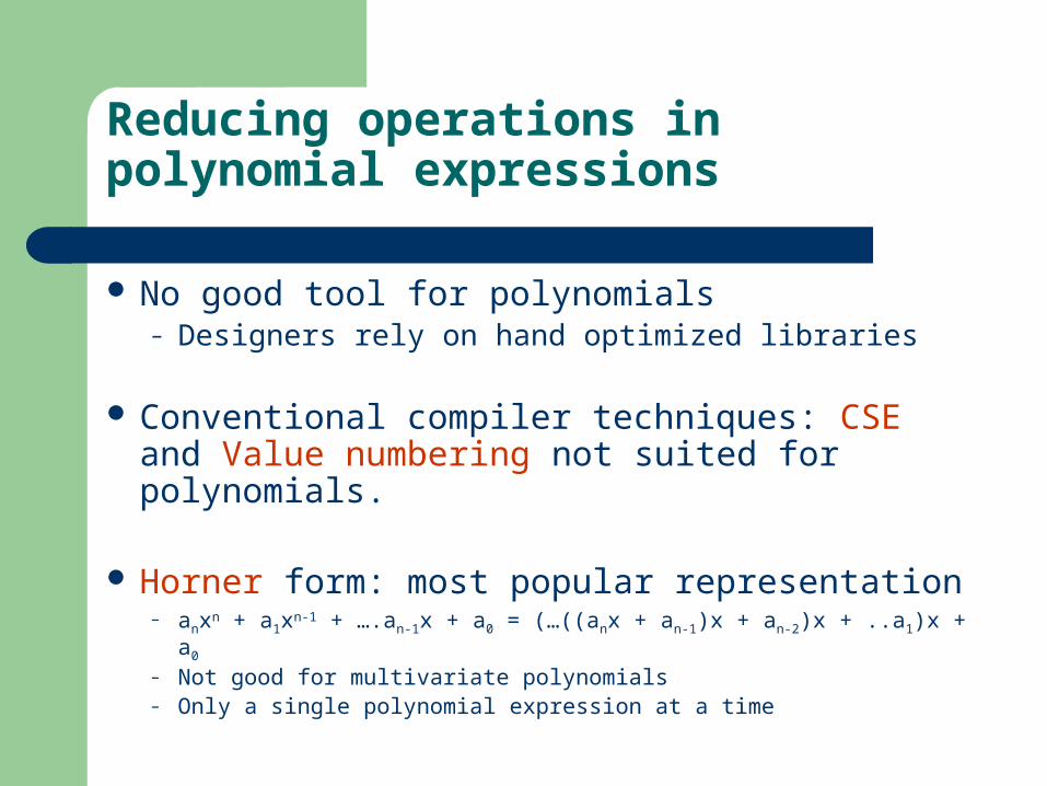
Reducing operations in polynomial expressions

No good tool for polynomials– Designers rely on hand optimized libraries

Conventional compiler techniques: CSE and Value numbering not suited for polynomials.

Horner form: most popular representation– anxn + a1xn-1 + ….an-1x + a0 = (…((anx + an-1)x + an-2)x + ..a1)x + a0

– Not good for multivariate polynomials– Only a single polynomial expression at a time

Comparison with Horner form

Quartic-spline polynomial (3-D graphics)P = zu4 + 4avu3 + 6bu2v2 + 4uv3w + qv4

Horner form (from MapleTM)P = zu4 + (4au3 + (6bu2 + (4uw + qv)v)v)v

(17 multiplications) Proposed algebraic method:

d1 = v2 ; d2 = d1*v

P = u3(uz + ad2) + d1( qd1 + u(wd2 + 6bu) )(11 multiplications)

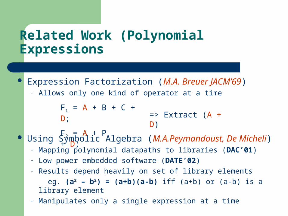
Related Work (Polynomial Expressions

Expression Factorization (M.A. Breuer JACM’69)– Allows only one kind of operator at a time

Using Symbolic Algebra (M.A.Peymandoust, De Micheli)– Mapping polynomial datapaths to libraries (DAC’01)– Low power embedded software (DATE’02)– Results depend heavily on set of library elements

eg. (a2 – b2) = (a+b)(a-b) iff (a+b) or (a-b) is a library element– Manipulates only a single expression at a time

F1 = A + B + C + D;

F2 = A + P + D;=> Extract (A + D)

Motivating Example

Consider set of expressions

Using CSE

yx– 4xy P

xyz– 4yz 4x P

zyx yx P

23

2

22

31

yx– 4xy P

xyz– 4yz 4x P

zyx yx P

23

2

22

31

xdydyd

xydzdyzd

xdzyddd

4 P

4 P

P

3133

2232

21

21211

xdydyd

xydzdyzd

xdzyddd

4 P

4 P

P

3133

2232

21

21211

16 multiplications and 4 additions/subtractions

12 multiplications and 4 additions/subtractions

Motivational Example

Using Horner transform

Using our algebraic technique

yx)x - (4y P

yz)x - (4 4yz P

)(y P

3

2

221

xyzz

yx)x - (4y P

yz)x - (4 4yz P

)(y P

3

2

221

xyzz

xyddd

xdzdd

yzxddxd

3323

2312

1311

P

4 - 4 P

P

xyddd

xdzdd

yzxddxd

3323

2312

1311

P

4 - 4 P

P

12 multiplications and 4 additions/subtractions

7 multiplications and 3 additions/subtractions

Introduction to algebraic technique for redundancy elimination

Algebraic techniques in multi-level logic synthesis (MLLS)– Decomposition, factoring reduce number of literals– Distill and Condense use Rectangle Covering methods

Polynomial Expressions (Our Technique)– Factoring, Single term common subexpressions reduces number of

multiplications– Multiple term common subexpressions reduces number of additions and

possibly multiplications

Key Differences (Generalization to handle higher orders)– Kernelling techniques– Finding single cube intersections

Introduction to our technique(Outline)

Find a subset of all possible subexpressions (kernel generation)

Transformation of Polynomial Expressions – Problem formulation

Extract multiple term common subexpressions and factors

Extract single term common factors

Introduction to our technique

Terminology– Literal: A variable or a constant eg. a,b,2,3.14– Cube: Product of literals e.g. +3a2b, -2a3b2c– SOP: Sum of cubes e.g. +3a2b – 2a3b2c– Cube-free expression: No literal or cube can divide

all the cubes of the expression– Kernel: A cube free sub-expression of an

expression, e.g. 3 – 2abc– Co-Kernel: A cube that is used to divide an

expression to get a kernel, e.g. a2b

Introduction to our Technique

Matrix Representation of Polynomial Expressions

– F = x3y – xy2z is represented by

– Each row represents a product term– Each column represents a variable/constant– Each element (i,j) represents power of variable j in term i

+/- x y z

+ 3 1 0

- 1 2 1

Generation of Kernels (example)

P1 = x3y + x2y2z {L} = {x,y,z}– Divide by x:

Ft = P1/x = x2y + xy2z

x y z

3 1 0

2 2 1

x y z

2 1 0

1 2 1

Generation of Kernels (example)

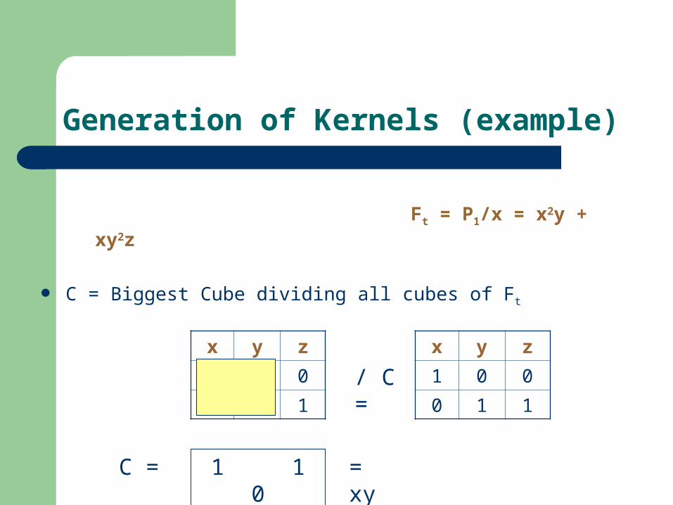
Ft = P1/x = x2y + xy2z

C = Biggest Cube dividing all cubes of Ft

x y z

2 1 0

1 2 1

1 1 0

/ C =

x y z

1 0 0

0 1 1

C = = xy

Generation of Kernels (example)

Obtain Kernel: F1 = Ft/C = (x2y + xy2z)/(xy) = ( x + yz)

Obtain Co-Kernel D1 = x*(xy) = x2y– No kernels within F1. Go back to P1

P1 = x3y + x2y2z– Divide now by next variable y

Ft = x3 + x2yz– C = x2

– But (x < y) ε C

Stop Here, to avoid repeating same kernel Ft/C = (x + yz)– No more kernels extracted– Record kernel F1 = P1 with co-kernel ‘1’

Concept of kernels and co-kernels

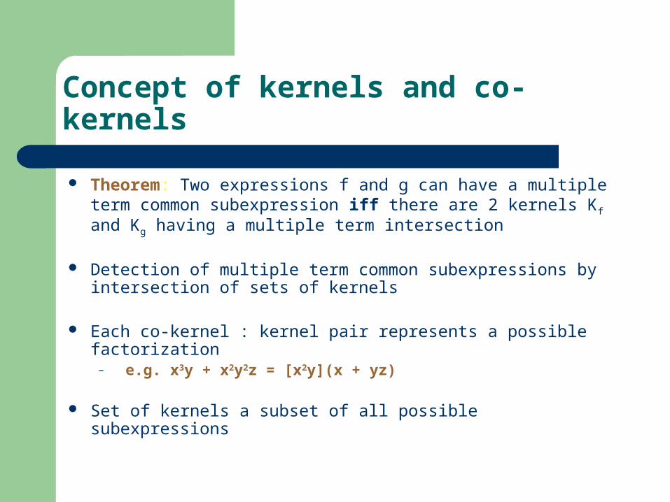
Theorem: Two expressions f and g can have a multiple term common subexpression iff there are 2 kernels Kf and Kg having a multiple term intersection

Detection of multiple term common subexpressions by intersection of sets of kernels

Each co-kernel : kernel pair represents a possible factorization– e.g. x3y + x2y2z = [x2y](x + yz)

Set of kernels a subset of all possible subexpressions

All Kernels and Co Kernels

yx– 4xy P

xyz– 4yz 4x P

zyx yx P

23

2

22

31

yx– 4xy P

xyz– 4yz 4x P

zyx yx P

23

2

22

31

Which kernels to choose?

)1](x - [4xy xy](x), - [4y : P

xyz](1) - 4yz [4x yz](4),[x yz](x), - [4 x](yz), - [4 : P

)1]([x ),yz](x [x : P

23

2

22321

y

zyxyy

)1](x - [4xy xy](x), - [4y : P

xyz](1) - 4yz [4x yz](4),[x yz](x), - [4 x](yz), - [4 : P

)1]([x ),yz](x [x : P

23

2

22321

y

zyxyy

Kernel Cube Matrix (KCM)

One row for each Kernel generated One column for each distinct kernel cube Each non-zero element represents a term

Kernel Cubes

x yz 4 -yz -xCoKernels

4 1(3) 1(4) 0 0 0

x2y 1(1) 1(2) 0 0 0

x 0 0 1(3) 1(5) 0

xy 0 0 1(6) 0 1(7)

yz 0 0 1(4) 0 1(5)

x3y

Finding Kernel Intersections(Distill Algorithm)

Each kernel intersection or factor appears as a rectangle– Rectangle: Set of rows and columns such that all

elements are ‘1’

Value of a rectangle = Weighted sum of the energy savings of the different operations

Goal: Maximum valued rectangular covering of KCM

Greedy heuristic: covering by prime rectangles

Modeling value function of a rectangle

Formula for weighted sum of energy savings on selection of a rectangle

R = # of rows ; C = # of columns M(Ri) = # of multiplications in row (co-kernel) i. M(Ci) = # of multiplications in column (kernel-cube) i m = ratio of average energy consumption of multiplication to addition in the target library

)1C()1R(

} ))C(M()1R())R(MR(1) - (C {mC

iR

i

)1C()1R(

} ))C(M()1R())R(MR(1) - (C {mC

iR

i

Value =

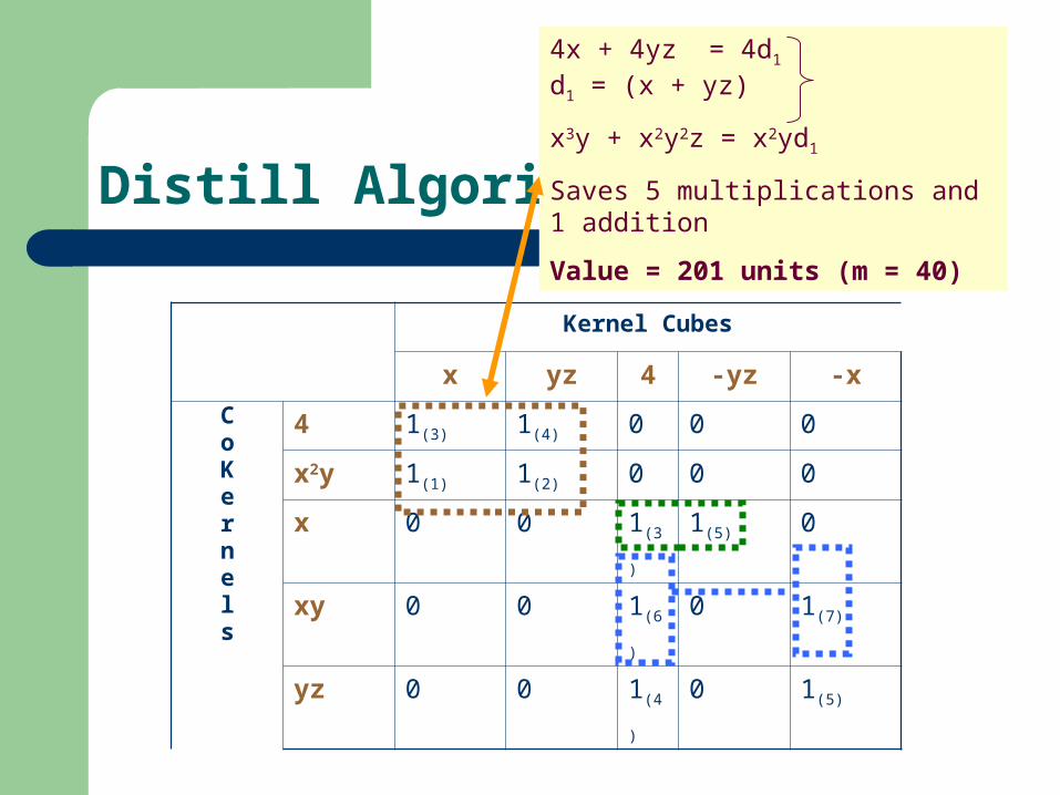
Distill Algorithm

Kernel Cubes

x yz 4 -yz -x

CoKernels

4 1(3) 1(4) 0 0 0

x2y 1(1) 1(2) 0 0 0

x 0 0 1(3) 1(5) 0

xy 0 0 1(6) 0 1(7)

yz 0 0 1(4) 0 1(5)

4x + 4yz = 4d1 d1 = (x + yz)

x3y + x2y2z = x2yd1

Saves 5 multiplications and 1 addition

Value = 201 units (m = 40)

Distill Algorithm

Kernel Cubes

x yz 4 -yz -x

CoKernels

4 1(3) 1(4) 0 0 0

x2y 1(1) 1(2) 0 0 0

x 0 0 1(3) 1(5) 0

xy 0 0 1(6) 0 1(7)

yz 0 0 1(4) 0 1(5)

Remove covered terms

4xy – x2y = xyd2

d2 = 4 – x

Saves 2 multiplications

Value = 80

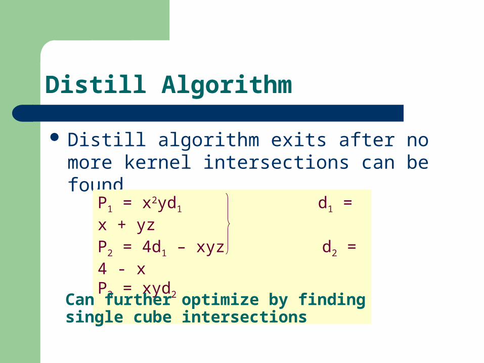
Distill Algorithm

Distill algorithm exits after no more kernel intersections can be found

P1 = x2yd1 d1 = x + yz

P2 = 4d1 – xyz d2 = 4 - xP3 = xyd2

Can further optimize by finding single cube intersections

Finding single cube intersections (Condense algorithm)

Form Cube Literal Matrix (CLM) – One row for each cube– One column for each literal– Eg. 2 cubes F1 = a4b3c; and F2 = a2b4c2

a b c

4 3 1

2 4 2

Finding single cube intersections (Condense algorithm)

Each (single term) common subexpression appears as a rectangle.

– Rectangle: Set of rows and columns where all elements are non-zero

Value of a rectangle is number of multiplications saved by selecting it

– C = cube corresponding to the rectangle Value = Rows*( (ΣC[i] ) -1)

Maximum valued rectangular covering will give minimum number of multiplications

Use greedy iterative covering by prime rectangles

Cube Literal Matrix (Condense Algorithm)

Literals

Term +/- x y z 4 d1 d2

Cubes

1 + 2 1 0 0 1 0

2 + 0 0 0 1 1 0

3 - 1 1 1 0 0 0

4 + 1 1 0 0 0 1

5 + 1 0 0 0 0 0

6 + 0 1 1 0 0 0

7 + 0 0 0 1 0 0

8 - 1 0 0 0 0 0

Save 2 multiplications by extracting xy

CLM for our example after Distill algorithm

C = xy

Condense AlgorithmExtracting xy

No more favorable cube intersections found

Literals

Term +/- x y z 4 d1 d2

Cubes

1 + 1 0 0 0 1 0

2 + 0 0 0 1 1 0

3 - 0 0 1 0 0 0

4 + 0 0 0 0 0 1

5 + 1 0 0 0 0 0

6 + 0 1 1 0 0 0

7 + 0 0 0 1 0 0

8 - 1 0 0 0 0 0

Final Implementation

– Total 7 multiplications, 3 additions/subtractions– Savings of 5 multiplications, 1 addition/subtraction

compared to CSE Impossible to obtain such results using conventional

techniques

xyddd

xdzdd

yzxddxd

3323

2312

1311

P

4 - 4 P

P

xyddd

xdzdd

yzxddxd

3323

2312

1311

P

4 - 4 P

P

Experimental setup

Polynomials used in Computer graphics and Signal Processing

1.0 µ technology library, characterized for power consumption

Synthesized using Synopsys Design CompilerTM – Min Hardware constraints (1 adder + 1 multiplier)– Med Hardware constraints (Max 4 multipliers)

Experimental setup

Estimated power using Synopsys Power CompilerTM for random inputs, using RTL Simulator (VCSTM)

Compared energy consumption with CSE and Horner form

Compared energy after voltage scaling

Results (Comparing operations)

Original CSE Horner Our

Technique

M A M A M A M A

ex1 23 4 16 4 17 4 13 4

ex2 34 5 22 5 23 5 16 5

ex3 32 8 18 8 18 8 11 8

ex4 43 17 24 17 19 17 17 17

ex5 34 6 23 6 20 6 13 6

Avg 33.2 8 20.6 8 19.4 8 14 8

Results (Min Hardware constraints)

Area Energy Energy-Delay Energy

(Scaled V)

C H C H C H C H

ex1 7.5 0.1 13.6 25.6 20.4 39.4 24.6 49.5

ex2 0.3 -4.2 21.6 29.3 39.0 48.8 52.2 64.6

ex3 -7.5 -24.2 29.4 10.4 47.6 25.9 62.2 36.9

ex4 5.6 2.5 37.0 28.7 57.1 46.1 74.3 59.8

ex5 3.7 2.0 44.8 36.8 62.8 54.8 78.3 69.7

Avg 1.9 -4.8 29.3 26.1 45.4 43.0 58.3 56.1

Results (Med Hardware constraints)

Area Energy Energy-Delay Energy

(Scaled V)

C H C H C H C H

ex1 30.5 3.9 16.1 39.2 9.7 44.1 9.7 55.0

ex2 14.8 1.0 9.7 29.6 20.3 58.7 22.7 75.4

ex3 8.3 3.7 42.5 29.1 44.9 37.0 51.8 45.0

ex4 8.9 9.0 28.2 29.5 39.5 40.6 47.4 48.3

ex5 8.0 6.6 41.4 40.8 58.4 59.7 72.6 75.9

Avg 14.1 4.9 27.6 33.6 34.6 48.0 40.8 60.0

Conclusions

Technique to reduce number of operations in polynomial expressions

Large savings in energy consumption observed over CSE and Horner methods

Need to consider scheduling and resource allocation to obtain further improvements

Conclusions

Thank you!! Questions ???

Extra slides

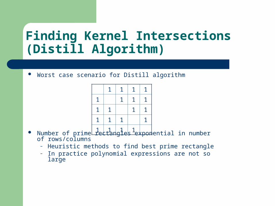
Finding Kernel Intersections(Distill Algorithm)

Worst case scenario for Distill algorithm

Number of prime rectangles exponential in number of rows/columns

– Heuristic methods to find best prime rectangle– In practice polynomial expressions are not so large

1 1 1 1

1 1 1 1

1 1 1 1

1 1 1 1

1 1 1 1