Energy-Efficient Deployment of Intelligent Mobile Sensor Networks

78 IEEE TRANSACTIONS ON SYSTEMS, MAN, AND CYBERNETICS—PART A: SYSTEMS AND HUMANS, VOL. 35, NO. 1, JANUARY 2005

Energy-Efficient Deployment of IntelligentMobile Sensor NetworksNojeong Heo and Pramod K. Varshney, Fellow, IEEE

Abstract—Many visions of the future include people immersedin an environment surrounded by sensors and intelligent devices,which use smart infrastructures to improve the quality of life andsafety in emergency situations. Ubiquitous communication enablesthese sensors or intelligent devices to communicate with each otherand the user or a decision maker by means of ad hoc wireless net-working. Organization and optimization of network resources areessential to provide ubiquitous communication for a longer du-ration in large-scale networks and are helpful to migrate intelli-gence from higher and remote levels to lower and local levels. Inthis paper, distributed energy-efficient deployment algorithms formobile sensors and intelligent devices that form an Ambient In-telligent network are proposed. These algorithms employ a syner-gistic combination of cluster structuring and a peer-to-peer deploy-ment scheme. An energy-efficient deployment algorithm based onVoronoi diagrams is also proposed here. Performance of our algo-rithms is evaluated in terms of coverage, uniformity, and time anddistance traveled until the algorithm converges. Our algorithmsare shown to exhibit excellent performance.

Index Terms—Ambient intelligence, deployment, distributedalgorithms, energy-efficiency, mobile wireless networks, wirelesssensor networks (WSN).

I. INTRODUCTION

DESIGN and deployment of infrastructured networks,such as a cellular network, has matured over the last two

decades. In such networks, mobile users access the network viafixed base stations. Planning and deployment of these networksis carried out based on radio propagation and terrain models,with the goal of maximizing radio coverage. More recently,there has been a great deal of interest in ad hoc networks.These networks employ fixed or mobile nodes and dynami-cally organize themselves into a network without requiring aninfrastructure. In ad hoc networks, each node acts not only asan end node, but also as a router. One important aspect in thedesign of these networks is the initialization procedure andestablishment of the routing structure. In these networks, a newparadigm is considered, where power usage instead of band-width is of primary concern. Extending system lifetime androbustness to unpredictable dynamics, rather than optimizingchannel throughput or minimizing the number of nodes, is thebiggest challenge during the design of these networks. Mostresearch on ad hoc networks has focused on issues such as the

Manuscript received October 20, 2003; revised March 9, 2004 and June 21,2004. This paper was recommended by Guest Editor G. L. Foresti.

The authors are with the Department of Electrical Engineering and Com-puter Science, Syracuse University, Syracuse, NY 13244 USA (e-mail:[email protected]; [email protected]; [email protected]).

Digital Object Identifier 10.1109/TSMCA.2004.838486

development of routing protocols and quality of service and noton topology and deployment.

Wireless sensor networks (WSN) that employ ad hoc net-working have become an area of intense research activity. Thisis due to the availability of inexpensive sensors for sensing andcontrol and technical advances in sensors, wireless communica-tions and networking, and signal processing. Many applicationsare envisaged including: environment and habitat monitoring;wild fire detection; inventory tracking; biomedical analysis; per-vasive computing; battlefield surveillance; and urban search-and-rescue operations, especially in hazardous situations. WSNoperate under limited radio coverage and attempt to conservebandwidth and battery power. Much research on this issue isunderway ranging from the development of power-saving hard-ware [18] to power-efficient medium access control (MAC) androuting protocols [11], [27], and to the development of col-laborative signal processing and power-aware algorithms [14].Sensor nodes are generally assumed to be fixed and randomlyplaced. The number of sensors is assumed to be quite large sothat coverage of the surveillance area is not an issue. Not muchattention has been paid to optimization in terms of the numberof nodes or their topology.

One of the key issues in this area is the deployment of mobilesensor nodes in the region of interest (ROI), where interestingevents might happen and the corresponding detection mecha-nism is required. Before a sensor can provide useful data tothe system, it must be deployed in a location that is contextu-ally appropriate. Optimum placement of sensors results in themaximum possible utilization of the available sensors [23]. Theproper choice for sensor locations based on application require-ments is difficult. The deployment of a static network is often ei-ther human monitored or random. Though many scenarios adoptrandom deployment for practical reasons such as deploymentcost and time, random deployment may not provide a uniformsensor distribution over the ROI, which is considered to be adesirable distribution in mobile sensor networks. Uneven nodetopology may lead to a short system lifetime. Self-deploymentmethods using mobile nodes [10], [25], [28] have been proposedto enhance network coverage and to extend the system lifetimevia configuration of uniformly distributed node topologies fromrandom node distributions. Since mobility itself requires en-ergy from its own limited energy source, a deployment schemeshould be designed carefully to minimize energy consumptionduring deployment, as well as to achieve certain goals, such assatisfactory coverage and/or an energy-efficient node topology.Moreover, it is desirable for a distributed sensor network node tohave a relatively simple hardware architecture, which requiresminimal computing power and memory. Each node should have

1083-4427/$20.00 © 2005 IEEE

Authorized licensed use limited to: University of Maryland Baltimore Cty. Downloaded on February 25,2010 at 09:38:22 EST from IEEE Xplore. Restrictions apply.

HEO AND VARSHNEY: ENERGY-EFFICIENT DEPLOYMENT OF INTELLIGENT MOBILE SENSOR NETWORKS 79

a simple and efficient algorithm for deployment, organization,and management of the network. Even though much researchon energy-efficient organization and management for the staticnode topology [23], [30] has been carried out, there has not beenany work on energy efficiency for deployment of mobile nodesto the best of our knowledge.

Deployment process itself is very energy consuming dueto the locomotive action as well as computation and commu-nications associated with it. Each node has a limited energysource. Not only minimizing average moving distance, but alsoreducing the difference of the remaining energy among sensornodes is essential for a longer system lifetime. Due to the dy-namic and distributed nature of deployment, it is a challengingtask to obtain full coverage in the ROI and to utilize energy ofeach sensor in a relatively fair fashion.

Previous research in distributed-sensor networking haslargely ignored sensor placement issues. Intelligent sensordeployment strategies are necessary to minimize cost and toprovide sufficient sensor coverage. In addition, sensor de-ployment must take into account the nature of the terrain,redundancy due to the likelihood of sensor failures, and thepower needed to transmit between deployed sensors.

The deployment of sensor networks varies with the applica-tion considered. It can be predetermined when the environmentis sufficiently known, in which case, the sensors can be strate-gically hand placed [2], [19], [22]. Schwiebert et al. [22] re-strict their investigation to an important class of WSN, namelybiomedical sensor networks, in which the locations of the sen-sors are fixed and the placement can be predetermined. Bia-gioni et al. [2] present and analyze a variety of regular de-ployment topologies, including circular and star deployments aswell as deployments in square, triangular, and hexagonal grids.There exists a close resemblance between the sensor-placementproblem and the traditional art gallery problem(AGP) in com-putational geometry [19]. The AGP seeks to determine the min-imal number of positions for guards or cameras so that everypoint in a gallery is observed by at least one guard or camera. Adeterministic solution can be found for the AGP and it appearsto be a possible solution to a variety of sensor-placement prob-lems. Even though there are many solutions to the AGP, all ofthem assume the availability of a good model of the environmenta priori. However, it is virtually impossible to have complete in-formation regarding the environment, where a WSN is likely tobe deployed. Furthermore, too much communication over longrange to obtain global information requires a huge amount ofenergy. This is an unaffordable burden on a system with limitedpower supply. Thus, deterministic deployment is impractical formany reasons, such as the harshness of the deployment regionthat may be remote, and inhospitable and the increased cost andlatency due to the large number of nodes deployed [23].

The deployment cannot be determined a priori when the en-vironment is unknown or hostile in which case the sensors maybe air-dropped from an aircraft [6] or deployed by other means,generally resulting in a random placement [9], [10], [17], [25].In this paper, the self-deployment of mobile sensor nodes is con-sidered. This is quite similar to problems considered in cooper-ative mobile robotics [5]. Mobile sensors are often desirable,since they can patrol a wide area, and can be repositioned for

better surveillance [21]. Some researchers have considered theuse of mobile robots in sensor networks. A recent work on mo-bile sensor networks [10] presents a distributed and scalable po-tential field-based approach for the deployment of mobile sen-sors. The fields are constructed such that each sensor is repelledby both obstacles and by other sensors, thereby forcing the net-work to spread itself through the environment. Winfield [25]considered autonomous dispersion of mobile nodes in a scenariowhere mobility is required to cover the entire region due to alack of wireless-network connectivity. He used a random diffu-sion method for node deployment while collecting data over afixed surveillance region. In the incremental deployment algo-rithm [9], nodes are added one at a time. The goal is to max-imize network coverage under the constraint that nodes main-tain line-of-sight with each other. Loo et al. considered a systemconsisting of a number of cooperating mobile nodes that movetoward a set of prioritized destinations under sensing and com-munication constraints [16]. They show how individual agentsknow when cooperation between agents improves the perfor-mance and when they should suspend cooperation.

A related problem to deployment in WSN is spatial local-ization [4]. In WSN, nodes need to be able to locate them-selves in various environments and on different distance scales.Meguerdichian et al. have considered the problem of locationand deployment of sensors in a WSN from a coverage stand-point [17]. The problems of coverage and deployment are funda-mentally interrelated. The authors define the coverage problemfrom different points of view, including deterministic, statis-tical, and the worst and best cases. They implicitly assumedfixed wireless sensor nodes. They argued that coverage is a pri-mary performance metric that provides an indication regardingquality-of-service. They combined computational geometry andgraph theoretic approaches to develop algorithms for coveragecalculations. Coverage in WSN, which is one of the main fo-cuses in this paper, will be discussed later in Section II. Bulusuet al.’s work [3] is somewhat similar to the deployment problemthat is considered here. They have investigated the problem ofadaptive beacon placement for localization in a WSN. They alsopointed out the lack of viability and inadequacy of fixed anddense beacon placement in some situations due to node per-turbation during deployment, noisy environment, and self-in-terference. By placing additional beacons incrementally, theyachieve empirical adaptation to terrain conditions. Unlike tradi-tional sensor systems, sensor networks depend on dense sensordeployment and physical colocation with their targets to accom-plish their goals. Dense deployment allows the use of redun-dancy [26], can reduce communication costs [20], and providessufficient number of nodes to allow physical colocation.

In this paper, three different deployment methods are pro-posed. First, a deployment algorithm for mobile nodes is pro-posed when each node is equally important and a peer-basedstructure is obtained. In many WSN scenarios, clustering is em-ployed to take advantage of local information and to reduce en-ergy consumption. An intelligent energy-efficient deploymentalgorithm for cluster-based WSN is proposed. The key idea ofthe second algorithm is the introduction of local clustering [12],[15] during the deployment process so as to increase the amountof local control over a fraction of the entire ROI. Each node



decides its own mode to be either in a clustering mode or apeer-to-peer mode based on its local environment such as thelocal density and the remaining energy level in a distributed andadaptive manner. Finally, an energy-efficient deployment algo-rithm based on Voronoi diagrams (VDs) is proposed.

The goal of the first method is different from prior work onthe deployment problem. The main objective of the first deploy-ment algorithm is topology improvement for longer system life-time by utilizing mobility of sensor nodes. A decision and con-trol mechanism is provided at each sensor during deployment,rather than random diffusion, which is used in Winfield’s work[25]. In contrast to Howard et al. [9], who use an incrementalapproach, the nodes in the first algorithm are deployed at thesame time and they organize themselves in an adaptive manner.Unlike Loo et al. [16], the first algorithm does not require pre-specified destinations to form an energy-efficient topology.

The significance of the second method is to provide a syn-ergistic combination of cluster structuring and peer-to-peerdeployment scheme in an intelligent manner in a hostile andunpredictable environment. The goals of our algorithm are therealization of the largest possible coverage area of the network,the formation of an energy-efficient node topology for a longersystem lifetime, and the organization of a hierarchical structurefor easier management and scalability that supports collabora-tion among nodes. These goals can be achieved by an adaptivecombination of two modes: clustering and peer-to-peer. In apeer-to-peer mode, each node moves itself to a sparse regionso that the coverage of the network may increase and/or anenergy-efficient node topology may be achieved. In a clusteringmode, each node follows the decision of the cluster-head so thateach node spends its energy in a balanced way and performscollaborative missions if necessary.

The significance of the third method is to provide an estimateof the lifetime of each node in a distributed fashion by usinglocal VDs. Each node can determine how long it can surviveand which action is more useful to its longevity for the currentnode topology during deployment. The best energy-utilizationpoint is obtained by comparing utility gains for movement todifferent possible node locations.

All three methods in this paper are based on the same as-sumptions shown in Section II but have different strengths forpossible applications. In practice, sensor capabilities may varydepending on the requirements for a certain task and the avail-able budget. The first method can achieve a quick deploymentwith simple sensors. The second method can establish clusteringstructure during deployment. The third method requires morecomputation, but shows local assessment of the performanceand high energy efficiency in mobility. The proper deploymentmethod can be chosen based on the requirements of the appli-cations and resources available.

Our deployment algorithms will be more useful in situationswhere it is hard to ensure precise initial deployment due to thefact that the deployment area is too dangerous or inaccessible tohumans. One can envisage an application involving a hazardousregion, where sensors mounted on mobile robots are deployedfrom an airborne vehicle [6]. These mobile robots then organizethemselves using algorithms presented in this paper. Randomlyscattered sensors over a battlefield or a hazardous site are not

Fig. 1. Sensor coverage models. (a) Binary sensor and (b) stochastic sensormodels.

likely to form a uniform distribution and provide desired cov-erage. Modification of WSN topology in an autonomous anddistributed manner using our algorithms can help in improvingcoverage and also to prolong expected system lifetime. This isessential in time-critical applications. For example, if an area iscontaminated by some hazardous material, a properly deployedsensor network can quickly sense and measure the amount ofhazardous material such as poisonous gas or nuclear leakage.By fully covering the entire area of interest, the overall condi-tion can be assessed quickly and this information can be usedfor search and rescue missions, as well as for evacuation-routeplanning. In some applications, initial sensor distributions maybe concentrated at specific points, such as elevators and stairs ina building.

In the next section, the sensor deployment problem is formu-lated. In Section III, performance metrics for a mobile WSNare discussed. The deployment algorithms are presented inSection IV followed by simulation results in Section V. Someconcluding remarks are provided in Section VI.

II. MOBILE-NODE DEPLOYMENT PROBLEM

In a WSN, physical placement or deployment of sensor nodesis needed prior to the initialization of a network for data acqui-sition and transmission using sensor nodes. The assumptionsmade in this paper are described and the deployment problemis formulated in this section.

It is assumed that all sensor nodes have identical capabil-ities for sensing, communication, computation, and mobility.Sensing coverage and communication coverage of each node isassumed to be ideal, which means that both coverage areas havea circular shape without any irregularity.

The coverage of each sensor can be defined either by a binarysensor model [23] or a stochastic sensor model [28] as shown inFig. 1. In the binary sensor model, the probability of detectionof the event of interest is one within the sensing range (sR),otherwise, the probability is zero. So the coverage of a sensornetwork using the binary sensor model is determined by findingthe union of the areas defined by the location of each sensorand its sR. In the stochastic sensor model, the probability ofdetection of the event of interest follows a decaying function ofdistance from the sensor. In this paper, the binary sensor modelis employed.

Computation capability is required at each node to supporta distributed algorithm that includes a reasoning and optimiza-tion process for deployment and routing. It is assumed that theinitial deployment is random and a distributed-deployment al-gorithm is executed starting from the initial random topology,using each node’s mobility. Another assumption is that everynode has the ability to know its own location by some method,



such as the global positioning system or iterative multilatera-tion [24]. This locationing ability is needed by each node, whilemaking a decision regarding its next movement in the deploy-ment process. Also, it is assumed that there are no errors duringtransmission of data and in the calculation of locations. It is fur-ther assumed that each node has only local information from theneighboring nodes within its direct communication range (cR).The cR of each node is defined by the maximum distance atwhich the signal-to-noise ratio is above a given threshold.

Without loss of generality, the deployment problem for a rect-angular ROI with a certain number of nodes that form an ad hocwireless network is considered. Each node has a limited amountof energy. The goal is to find the positions and movements ofnodes to achieve maximum coverage and to form a uniformlydistributed wireless network in minimum time and with min-imum energy consumption. A suite of heuristic algorithms aredeveloped for this problem and their performances are evaluatedin terms of the performance metrics: coverage, uniformity, andthe time and distance traveled until convergence. These metricsare described next.

III. PERFORMANCE METRICS IN MOBILE WSN

The selection of suitable measures to compare performancesof different approaches and resulting solutions is an importantissue in a mobile WSN. Coverage, uniformity, and time anddistance traveled prior to convergence are considered as per-formance metrics in mobile WSN here. Coverage and unifor-mity are related to the performance of sensor networks after thedeployment of sensors is complete. Time and distance traveledprior to convergence are directly related to the performance ofthe deployment scheme itself.

A. Coverage

Generally, coverage can be considered as the measure ofquality of service of a sensor network. The concept of coverageas a paradigm for the system-level functionality of multirobotsystems was introduced by Gage [7], [31].

In this paper, coverage [9] is defined as the ratio of the unionof areas (in square meters) covered by each node and the area(in square meters) of the entire ROI. Here, the covered area ofeach node is defined as the circular area within its sensing radius

. Perfect detection of all interesting events in the covered areais assumed

whereis the area covered by the th node;is the total number of nodes;stands for the area of the ROI.

If a node is located well inside the ROI, its complete coveragearea will lie within the ROI. In this case, the full area of thatcircle, i.e., , is included in the covered region. If a nodeis located near the boundary of the ROI, then only the part ofthe ROI covered by that node is included in the computation.Because of the areas covered by nodes that fall out of the ROI

and the overlap of covered areas between nodes, one needs touse more nodes than simply the ratio of and the area sensedby a single node.

The overall coverage of a sensor network is composed of thecovered regions of each sensor node. Though the coverage ofa sensor is expressed by a sensor model which is binary or sto-chastic, the overall coverage of a sensor network depends on thelocations of the sensor nodes in the sensor field. The topologyincluding the locations and spacing of sensor nodes determinesthe overall coverage of the network as well as the expected life-time of the network.

sR and cR of a node are distinguished in the paper. In gen-eral, they will be different and accordingly sensing coverage andcommunication coverage will be different. Sensing coveragecan be accrued when sensor nodes are connected via wirelesslinks. If the network is separated by any reason, the area cov-ered by the subnets that do not have wireless links to the sinknode is lost.

B. Uniformity

Uniformly distributed-sensor nodes spend energy moreevenly through the WSN than sensor nodes with an irregulartopology. When the distances between nodes become similar,each node can utilize its resources efficiently with the minimumuse of its power and an increased throughput, due to reductionof the interferences between nodes. So, uniformity of networktopology can be used as a good estimator for the expectedsystem lifetime. Also, fewer nodes are required to cover an ROIwhen nodes are more evenly distributed.

Uniformity can be defined as the average local standard de-viation of the distances between nodes

whereis the total number of nodes;is the number of neighbors of the th node;is the distance between th and th nodes;is the mean of internodal distances between the thnode and its neighbors.

In the calculation of local uniformity at the th node, onlyneighboring nodes that reside within its cR are considered.The uniformity measure is a local measure and is computedlocally because each node has access to local information only.A smaller value of means that nodes are more uniformlydistributed in the ROI. In uniformly distributed networks,internodal distances are almost the same; the expected energyconsumption per communication as well as the expected life-time of each node is almost the same if the nodes were identicaland have the same amount of energy initially. Therefore, it isexpected to have full energy utilization at each node and longersystem lifetime for uniformly distributed networks.



C. Time

The time spent for deployment [9] is also important in manytime-critical applications, such as search-and-rescue and dis-aster recovery operations. Mostly, the required time dependson the complexity of the reasoning and optimization algorithmand physical time for the movement of nodes. The total timeelapsed is defined here as the time elapsed until all the nodesreach their final locations. This paper focuses on the time spentfor deployment itself and not on data-transmission delays froma source node to a destination node that is commonly used fornetwork-performance evaluation and its quality of service.

D. Distance

The average distance traveled [9] by each node is related tothe energy required for its movement. So, the expected distancetraveled is important for the estimation of energy (fuel) requiredwhen each node has a limited energy supply. The variance of thedistance traveled is also important to determine the fairness ofthe deployment algorithm and for system energy utilization. Ifthe variance of distance traveled is large, the variance of energyremaining also is large. The nodes that have less energy thanother nodes exhaust their energy early. Early dead nodes resultin a loss of coverage and the remaining nodes may require anincreased transmission range or a longer routing path.

IV. ALGORITHMS

In this paper, three different deployment methods are pre-sented. The first method operates in a peer-to-peer mode, whereeach node is considered to be equal. The second method is a syn-ergistic combination of the peer-to-peer method with a cluster-based method. Clustering, a hierarchical networking concept, isemployed in many WSN scenarios to take advantage of localinformation and to reduce energy consumption. Finally, an en-ergy-efficient deployment algorithm based on VDs is proposed.

A. Distributed Self-Spreading Algorithm (DSSA)

The peer to peer algorithm which is called the DSSA is in-spired by the equilibrium of molecules, which minimizes molec-ular electronic energy and internuclear repulsion. Each particledetermines its own lowest energy point in a distributed mannerand its resulting spacing from the other particles is almost thesame. While deploying a WSN using mobile nodes, one ob-serves that one has an analogous problem. If sensors are locatedtoo close to each other, the gain in coverage from additional sen-sors is not high. On the contrary, if sensors are located too farfrom each other, the coverage regions may not overlap and maycause a partitioning of the network. Both situations are similar tointernuclear repulsion and attractions between molecules. Op-timal spacing between sensors in the sense of coverage can befound by a process similar to the equilibrium of molecules.

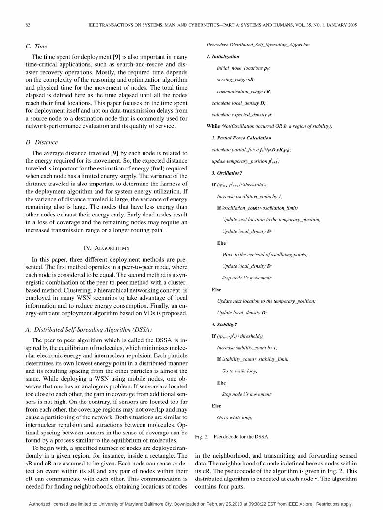
To begin with, a specified number of nodes are deployed ran-domly in a given region, for instance, inside a rectangle. ThesR and cR are assumed to be given. Each node can sense or de-tect an event within its sR and any pair of nodes within theircR can communicate with each other. This communication isneeded for finding neighborhoods, obtaining locations of nodes

Fig. 2. Pseudocode for the DSSA.

in the neighborhood, and transmitting and forwarding senseddata. The neighborhood of a node is defined here as nodes withinits cR. The pseudocode of the algorithm is given in Fig. 2. Thisdistributed algorithm is executed at each node . The algorithmcontains four parts.



1) Initialization: In the initialization part, the values of cR,sR, and the initial node locations are specified. The cR andsR are assumed to be given. Initial node locations are spec-ified in terms of a vector that contains the longitude componentand the latitude component of each node location, and is as-sumed to follow a random distribution. Extension to higher di-mensions is possible by adding more components in the positionvector. A quantity called expected density, which is a rough es-timate of the desired density, is required in the algorithm. Thiscan be calculated by using cR cR , whereis the number of nodes, cR is the cR of each node, and is thearea of the ROI. Thus, expected density is the average numberof nodes required to cover the entire area when these nodes aredeployed uniformly. Initial local density of a node is equalto the number of nodes within its cR. These densities will beused when decisions regarding positions of nodes are made.

2) Partial Force Calculation: The concept of force is intro-duced to define the movement of nodes during the deploymentprocess. The force is dependent on not only the distance be-tween the nodes but also the current local density. The forcecorresponding to high local density is greater than the force cor-responding to low local density. The force from a node that iscloser is greater than that from a node that is farther, which issimilar to the movements of the particles in physics that followCoulomb’s Law.

A force function is defined which satisfies the followingconditions.

i) Inverse relation: , when , whereand are node separations from the origin. The node

under consideration is assumed to be at the origin.ii) Upper bound: .iii) Lower bound: , where cR, is the node

separation and cR is the communication range of eachnode.

Condition (i) is the same as in physics, but conditions (ii)and (iii) are included to modify the model to incorporate thenotion of locality. In other words, a limiting function is appliedvia conditions (ii) and (iii).

The partial force at time step on the th node from the thnode that is in the neighborhood of the th node is calculated tobe a repulsive force as

cR (1)

wherestands for the location of the th node at time step ;stands for the local density of the th node at timestep .

The density factor , which is defined as the ratio ofthe local density and the square of the expected densityat each node, is small in sparse regions and is large in dense re-gions. Its inclusion in the force function expedites the processof node spreading. Also, internodal distance affects the par-tial force inversely. Closely located nodes impose larger partialforces and nodes that are far apart induce smaller partial forceson each other. The magnitude of the partial force exerted by a

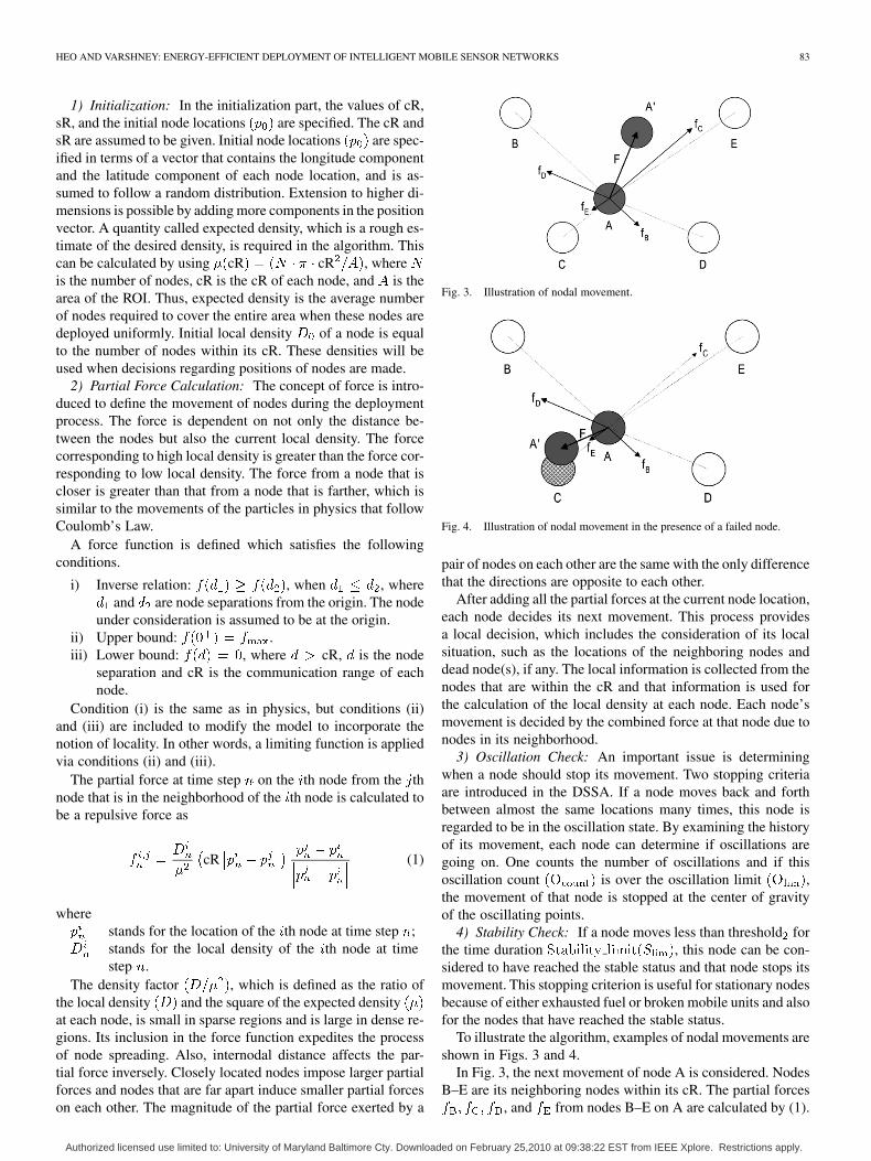
Fig. 3. Illustration of nodal movement.

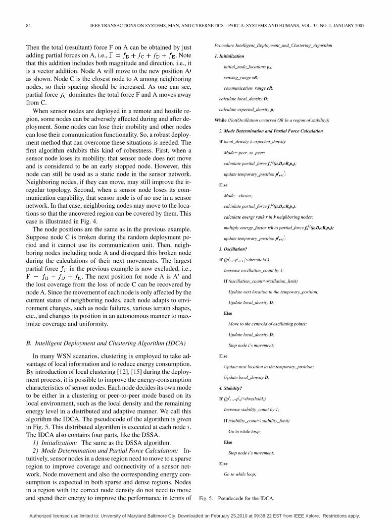
Fig. 4. Illustration of nodal movement in the presence of a failed node.

pair of nodes on each other are the same with the only differencethat the directions are opposite to each other.

After adding all the partial forces at the current node location,each node decides its next movement. This process providesa local decision, which includes the consideration of its localsituation, such as the locations of the neighboring nodes anddead node(s), if any. The local information is collected from thenodes that are within the cR and that information is used forthe calculation of the local density at each node. Each node’smovement is decided by the combined force at that node due tonodes in its neighborhood.

3) Oscillation Check: An important issue is determiningwhen a node should stop its movement. Two stopping criteriaare introduced in the DSSA. If a node moves back and forthbetween almost the same locations many times, this node isregarded to be in the oscillation state. By examining the historyof its movement, each node can determine if oscillations aregoing on. One counts the number of oscillations and if thisoscillation count is over the oscillation limit ,the movement of that node is stopped at the center of gravityof the oscillating points.

4) Stability Check: If a node moves less than threshold forthe time duration , this node can be con-sidered to have reached the stable status and that node stops itsmovement. This stopping criterion is useful for stationary nodesbecause of either exhausted fuel or broken mobile units and alsofor the nodes that have reached the stable status.

To illustrate the algorithm, examples of nodal movements areshown in Figs. 3 and 4.

In Fig. 3, the next movement of node A is considered. NodesB–E are its neighboring nodes within its cR. The partial forces

, and from nodes B–E on A are calculated by (1).



Then the total (resultant) force F on A can be obtained by justadding partial forces on A, i.e., . Notethat this addition includes both magnitude and direction, i.e., itis a vector addition. Node A will move to the new position Aas shown. Node C is the closest node to A among neighboringnodes, so their spacing should be increased. As one can see,partial force dominates the total force F and A moves awayfrom C.

When sensor nodes are deployed in a remote and hostile re-gion, some nodes can be adversely affected during and after de-ployment. Some nodes can lose their mobility and other nodescan lose their communication functionality. So, a robust deploy-ment method that can overcome these situations is needed. Thefirst algorithm exhibits this kind of robustness. First, when asensor node loses its mobility, that sensor node does not moveand is considered to be an early stopped node. However, thisnode can still be used as a static node in the sensor network.Neighboring nodes, if they can move, may still improve the ir-regular topology. Second, when a sensor node loses its com-munication capability, that sensor node is of no use in a sensornetwork. In that case, neighboring nodes may move to the loca-tions so that the uncovered region can be covered by them. Thiscase is illustrated in Fig. 4.

The node positions are the same as in the previous example.Suppose node C is broken during the random deployment pe-riod and it cannot use its communication unit. Then, neigh-boring nodes including node A and disregard this broken nodeduring the calculations of their next movements. The largestpartial force in the previous example is now excluded, i.e.,

. The next position for node A is A andthe lost coverage from the loss of node C can be recovered bynode A. Since the movement of each node is only affected by thecurrent status of neighboring nodes, each node adapts to envi-ronment changes, such as node failures, various terrain shapes,etc., and changes its position in an autonomous manner to max-imize coverage and uniformity.

B. Intelligent Deployment and Clustering Algorithm (IDCA)

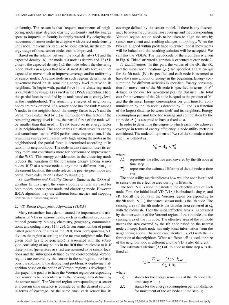
In many WSN scenarios, clustering is employed to take ad-vantage of local information and to reduce energy consumption.By introduction of local clustering [12], [15] during the deploy-ment process, it is possible to improve the energy-consumptioncharacteristics of sensor nodes. Each node decides its own modeto be either in a clustering or peer-to-peer mode based on itslocal environment, such as the local density and the remainingenergy level in a distributed and adaptive manner. We call thisalgorithm the IDCA. The pseudocode of the algorithm is givenin Fig. 5. This distributed algorithm is executed at each node .The IDCA also contains four parts, like the DSSA.

1) Initialization: The same as the DSSA algorithm.2) Mode Determination and Partial Force Calculation: In-

tuitively, sensor nodes in a dense region need to move to a sparseregion to improve coverage and connectivity of a sensor net-work. Node movement and also the corresponding energy con-sumption is expected in both sparse and dense regions. Nodesin a region with the correct node density do not need to moveand spend their energy to improve the performance in terms of Fig. 5. Pseudocode for the IDCA.



uniformity. The reason is that frequent movements of neigh-boring nodes may degrade existing uniformity and the energyspent to improve uniformity is simply wasted. By delaying themovement of sensor nodes in a region with correct node densityuntil nodal movements stabilize to some extent, inefficient en-ergy usage of those sensor nodes can be improved.

Based on the relation between the local density ( ) and theexpected density , the mode at a node is determined. If isclose to the expected density , the node selects the clusteringmode. Nodes in regions that have desired density levels are notexpected to move much to improve coverage and/or uniformityof sensor nodes. A sensor node in such regions determines itsmovement based on its remaining energy level relative to itsneighbors. To begin with, partial force in the clustering modeis calculated by using (1) as used in the DSSA algorithm. Then,this partial force is modified by its rank based on its energy levelin the neighborhood. The remaining energies of neighboringnodes are rank ordered. If a sensor node has the rank among

nodes in the neighborhood, the energy factor is and thepartial force calculated by (1) is multiplied by this factor. If theremaining energy level is low, the partial force of the node willbe smaller than that used in DSSA based on its energy factorin its neighborhood. The node in this situation saves its energyand contributes less to WSN performance improvement. If theremaining energy level is relatively high among the nodes in theneighborhood, the partial force is determined according to itsrank in its neighborhood. The node in this situation uses its en-ergy more and contributes more for performance improvementof the WSN. This energy consideration in the clustering modereduces the variation of the remaining energy among sensornodes. If of a sensor node at any time is different than atthe current location, this node selects the peer-to-peer mode andpartial force calculation is done by using (1).

3) Oscillation and Stability Checks: Same as the DSSA al-gorithm. In this paper, the same stopping criteria are used forboth modes: peer to peer mode and clustering mode. However,IDCA algorithm may use different local metrics and stoppingcriteria in a clustering mode.

C. VD-Based Deployment Algorithm (VDDA)

Many researchers have demonstrated the importance and use-fulness of VDs in various fields, such as mathematics, compu-tational geometry, biology, chemistry, geography, communica-tions, and coding theory [1], [29]. Given some number of pointscalled generators or sites in the ROI, their corresponding VDdivides the region according to the nearest-neighbor rule. Eachgiven point (a site or generator) is associated with the subre-gion consisting of any points in the ROI that are closest to it. Ifthese points (generators or sites) are assumed to be sensor loca-tions and the subregions defined by the corresponding Voronoiregions are covered by the sensor in the subregion, one has apossible solution to the deployment problem. A deployment al-gorithm based on the notion of Voronoi regions is developed. Inthis paper, the goal is to have the Voronoi region correspondingto a sensor to be coincident with the coverage area defined bythe sensor model. The Voronoi region corresponding to a sensorat a certain time instance is considered as the desired solutionin terms of coverage. At the same time, each sensor has its

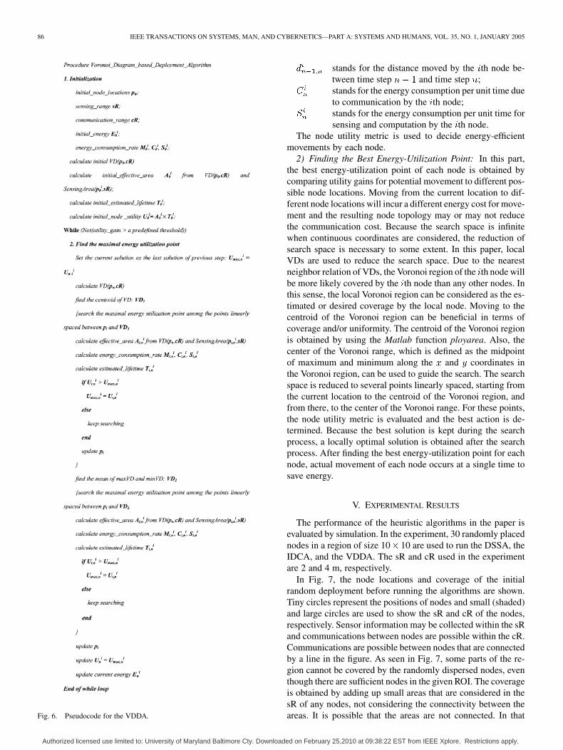
coverage defined by the sensor model. If there is any discrep-ancy between the current sensor coverage and the correspondingVoronoi region, action needs to be taken to align the two bysensor movement and resulting changes in topology. When thetwo are aligned within predefined tolerance, nodal movementswill be halted and the resulting solution will be accepted. Wecall this the VDDA. The pseudocode of the algorithm is givenin Fig. 6. This distributed algorithm is executed at each node .

1) Initialization: In this part, the values of the cR, the sR,and the initial node locations are specified. Initial energyfor the th node is specified and each node is assumed tohave the same amount of energy in the beginning. Energy con-sumption for different activities is specified. Energy consump-tion for movement of the th node is specified in terms ofdefined as the cost for movement per unit distance. The totalcost for movement of the th node is equal to the product ofand the distance. Energy consumption per unit time for com-munication by the th node is denoted by and is a functionof the largest distance between itself and its neighbors. Energyconsumption per unit time for sensing and computation by theth node is assumed to have a fixed cost.

In order to determine the degree to which each node achievescoverage in terms of energy efficiency, a node utility metric isconsidered. The node utility metric of the th node at timestep is defined as

whererepresents the effective area covered by the th node attime step ;represents the estimated lifetime of the th node at timestep .

The node utility metric indicates how well the node is utilizedto sense over its effective area during its lifetime.

The local VD is used to calculate the effective area of eachnode. First, the initial local VD is obtained using andcR. For all the points in the Voronoi region corresponding tothe th node , the nearest sensor node is the th node. Thesensing area of the th node is the circular area centered atwith the radius sR. Then the initial effective area is obtainedby the intersection of the Voronoi region of the th node and thesensing area of the th node. The effective area of the th nodemeans the area covered by the th node based on the nearestnode concept. Each node has only local information from theneighboring nodes. The node can calculate its VD with the in-formation of the neighbors. When a different cR is used, the sizeof the neighborhood is different and the VD is also different.

The estimated lifetime of th node at time step is de-fined as

wherestands for the energy remaining at the th node aftertime step ;stands for the energy consumption per unit distancefor movement of the th node at time step ;



Fig. 6. Pseudocode for the VDDA.

stands for the distance moved by the th node be-tween time step and time step ;stands for the energy consumption per unit time dueto communication by the th node;stands for the energy consumption per unit time forsensing and computation by the th node.

The node utility metric is used to decide energy-efficientmovements by each node.

2) Finding the Best Energy-Utilization Point: In this part,the best energy-utilization point of each node is obtained bycomparing utility gains for potential movement to different pos-sible node locations. Moving from the current location to dif-ferent node locations will incur a different energy cost for move-ment and the resulting node topology may or may not reducethe communication cost. Because the search space is infinitewhen continuous coordinates are considered, the reduction ofsearch space is necessary to some extent. In this paper, localVDs are used to reduce the search space. Due to the nearestneighbor relation of VDs, the Voronoi region of the th node willbe more likely covered by the th node than any other nodes. Inthis sense, the local Voronoi region can be considered as the es-timated or desired coverage by the local node. Moving to thecentroid of the Voronoi region can be beneficial in terms ofcoverage and/or uniformity. The centroid of the Voronoi regionis obtained by using the Matlab function ployarea. Also, thecenter of the Voronoi range, which is defined as the midpointof maximum and minimum along the and coordinates inthe Voronoi region, can be used to guide the search. The searchspace is reduced to several points linearly spaced, starting fromthe current location to the centroid of the Voronoi region, andfrom there, to the center of the Voronoi range. For these points,the node utility metric is evaluated and the best action is de-termined. Because the best solution is kept during the searchprocess, a locally optimal solution is obtained after the searchprocess. After finding the best energy-utilization point for eachnode, actual movement of each node occurs at a single time tosave energy.

V. EXPERIMENTAL RESULTS

The performance of the heuristic algorithms in the paper isevaluated by simulation. In the experiment, 30 randomly placednodes in a region of size 10 10 are used to run the DSSA, theIDCA, and the VDDA. The sR and cR used in the experimentare 2 and 4 m, respectively.

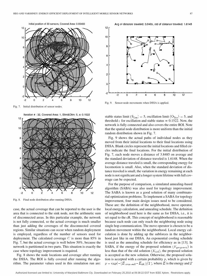
In Fig. 7, the node locations and coverage of the initialrandom deployment before running the algorithms are shown.Tiny circles represent the positions of nodes and small (shaded)and large circles are used to show the sR and cR of the nodes,respectively. Sensor information may be collected within the sRand communications between nodes are possible within the cR.Communications are possible between nodes that are connectedby a line in the figure. As seen in Fig. 7, some parts of the re-gion cannot be covered by the randomly dispersed nodes, eventhough there are sufficient nodes in the given ROI. The coverageis obtained by adding up small areas that are considered in thesR of any nodes, not considering the connectivity between theareas. It is possible that the areas are not connected. In that



Fig. 7. Initial distribution of sensor nodes.

Fig. 8. Final node distribution after running DSSA.

case, the actual coverage that can be reported to the user is thearea that is connected to the sink node, not the arithmetic sumof disconnected areas. In this particular example, the networkis not fully connected, so the actual coverage is much smallerthan just adding the coverages of the disconnected coveredregions. Similar situations can occur when random deploymentis employed, regardless of the number of sensors used fordeployment. The calculated coverage is more than 85% inFig. 7, but the actual coverage is well below 50%, because thenetwork is partitioned in two parts. This situation is exactly thecase where topology improvement is required.

Fig. 8 shows the node locations and coverage after runningthe DSSA. The ROI is fully covered after running the algo-rithm. The parameter values used in this simulation run are:

Fig. 9. Sensor-node movements when DSSA is applied.

stable status limit 5, oscillation limit 5, andthreshold for oscillation and stable status 0.1522. Now, thenetwork is fully connected and also covers the entire ROI. Notethat the spatial node distribution is more uniform than the initialrandom distribution shown in Fig. 7.

Fig. 9 shows the actual paths of individual nodes as theymoved from their initial locations to their final locations usingDSSA. Blank circles represent the initial locations and filled cir-cles indicate the final locations. For the initial distribution ofFig. 7, each node moves a distance of 3.8485 on average andthe standard deviation of distance traveled is 1.6148. When theaverage distance traveled is small, the corresponding energy forlocomotion is small. Also, when the standard deviation of dis-tance traveled is small, the variation in energy remaining at eachnode is not significant and a longer system lifetime with full cov-erage can be expected.

For the purpose of comparison, a simulated annealing-basedalgorithm (SABA) was also used for topology improvement.The SABA is known as a good solution of many combinato-rial optimization problems. To implement a SABA for topologyimprovement, four main design issues need to be considered.These are: the definition of the neighborhood, move operator,local energy calculation, and annealing schedule. The definitionof neighborhood used here is the same as for DSSA, i.e., it isset equal to the cR. This concept of neighborhood is reasonablebecause each node can only reach the neighboring node usingsingle hop communication. The move operator is chosen to be arandom movement within the neighborhood. Local energy cal-culation is done by adding up the subforces in the neighbor-hood just like in our DSSA. An exponential cooling scheduleis used as the annealing schedule for efficiency as in [13]. InSABA, if the energy of the proposed solution isless than that of the old solution , the proposed solutionis accepted as the new solution. Otherwise, the proposed solu-tion is accepted with a certain probability , which is given by

, where is the energy and



Fig. 10. Final node distribution after running SABA.

Fig. 11. Node movements when SABA is applied.

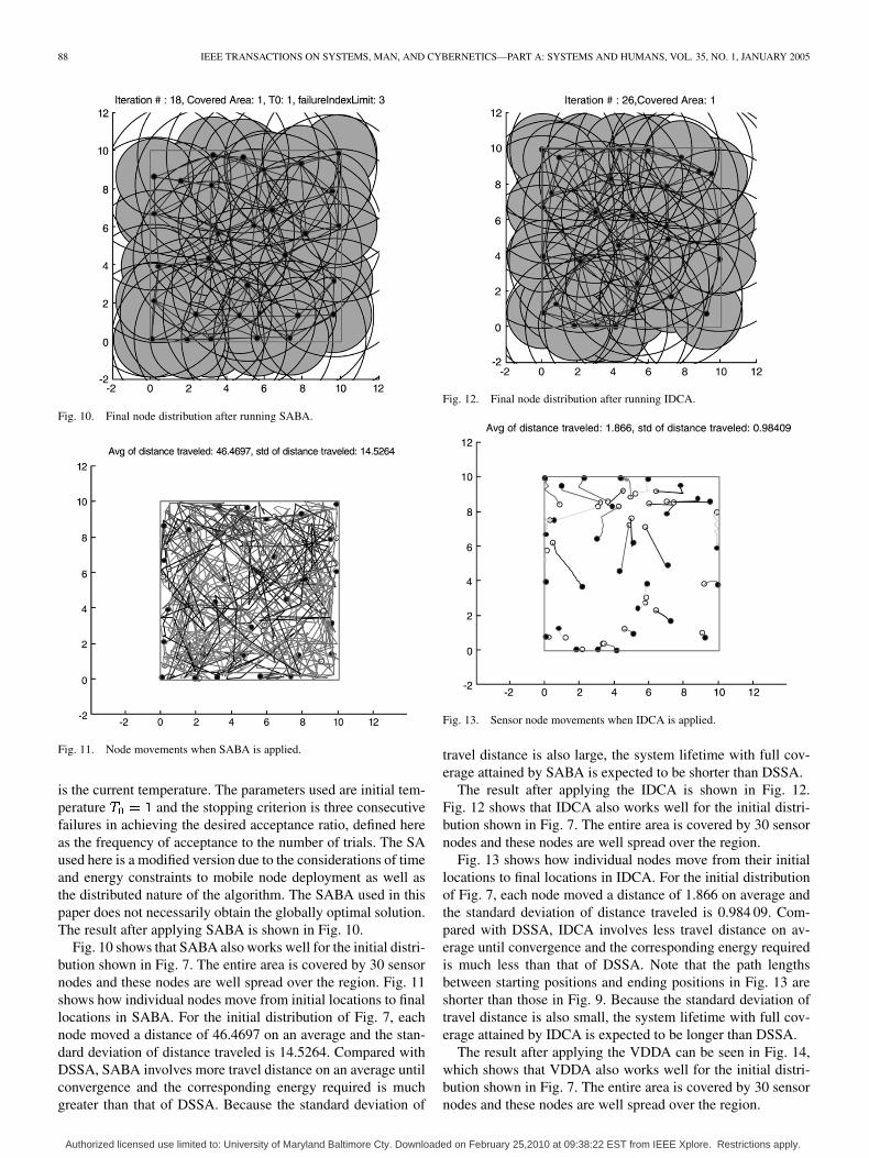
is the current temperature. The parameters used are initial tem-perature and the stopping criterion is three consecutivefailures in achieving the desired acceptance ratio, defined hereas the frequency of acceptance to the number of trials. The SAused here is a modified version due to the considerations of timeand energy constraints to mobile node deployment as well asthe distributed nature of the algorithm. The SABA used in thispaper does not necessarily obtain the globally optimal solution.The result after applying SABA is shown in Fig. 10.

Fig. 10 shows that SABA also works well for the initial distri-bution shown in Fig. 7. The entire area is covered by 30 sensornodes and these nodes are well spread over the region. Fig. 11shows how individual nodes move from initial locations to finallocations in SABA. For the initial distribution of Fig. 7, eachnode moved a distance of 46.4697 on an average and the stan-dard deviation of distance traveled is 14.5264. Compared withDSSA, SABA involves more travel distance on an average untilconvergence and the corresponding energy required is muchgreater than that of DSSA. Because the standard deviation of

Fig. 12. Final node distribution after running IDCA.

Fig. 13. Sensor node movements when IDCA is applied.

travel distance is also large, the system lifetime with full cov-erage attained by SABA is expected to be shorter than DSSA.

The result after applying the IDCA is shown in Fig. 12.Fig. 12 shows that IDCA also works well for the initial distri-bution shown in Fig. 7. The entire area is covered by 30 sensornodes and these nodes are well spread over the region.

Fig. 13 shows how individual nodes move from their initiallocations to final locations in IDCA. For the initial distributionof Fig. 7, each node moved a distance of 1.866 on average andthe standard deviation of distance traveled is 0.984 09. Com-pared with DSSA, IDCA involves less travel distance on av-erage until convergence and the corresponding energy requiredis much less than that of DSSA. Note that the path lengthsbetween starting positions and ending positions in Fig. 13 areshorter than those in Fig. 9. Because the standard deviation oftravel distance is also small, the system lifetime with full cov-erage attained by IDCA is expected to be longer than DSSA.

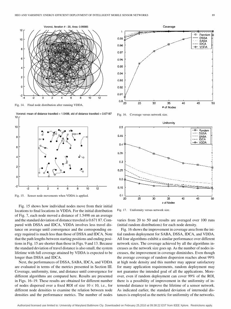
The result after applying the VDDA can be seen in Fig. 14,which shows that VDDA also works well for the initial distri-bution shown in Fig. 7. The entire area is covered by 30 sensornodes and these nodes are well spread over the region.



Fig. 14. Final node distribution after running VDDA.

Fig. 15. Sensor node movements when VDDA is applied.

Fig. 15 shows how individual nodes move from their initiallocations to final locations in VDDA. For the initial distributionof Fig. 7, each node moved a distance of 1.5498 on an averageand the standard deviation of distance traveled is 0.671 87. Com-pared with DSSA and IDCA, VDDA involves less travel dis-tance on average until convergence and the corresponding en-ergy required is much less than those of DSSA and IDCA. Notethat the path lengths between starting positions and ending posi-tions in Fig. 15 are shorter than those in Figs. 9 and 13. Becausethe standard deviation of travel distance is also small, the systemlifetime with full coverage attained by VDDA is expected to belonger than DSSA and IDCA.

Next, the performances of DSSA, SABA, IDCA, and VDDAare evaluated in terms of the metrics presented in Section III.Coverage, uniformity, time, and distance until convergence fordifferent algorithms are compared here. Results are presentedin Figs. 16–19. These results are obtained for different numberof nodes dispersed over a fixed ROI of size 10 10, i.e., fordifferent node densities to examine the relation between nodedensities and the performance metrics. The number of nodes

Fig. 16. Coverage versus network size.

Fig. 17. Uniformity versus network size.

varies from 20 to 50 and results are averaged over 100 runs(initial random distributions) for each node density.

Fig. 16 shows the improvement in coverage area from the ini-tial random deployment for SABA, DSSA, IDCA, and VDDA.All four algorithms exhibit a similar performance over differentnetwork sizes. The coverage achieved by all the algorithms in-creases as the network size goes up. As the number of nodes in-creases, the improvement in coverage diminishes. Even thoughthe average coverage of random dispersion reaches about 99%at high node density and this number may appear satisfactoryfor many application requirements, random deployment maynot guarantee the intended goal of all the applications. More-over, even if random deployment can cover 99% of the ROI,there is a possibility of improvement in the uniformity of in-ternodal distance to improve the lifetime of a sensor network.As indicated earlier, the standard deviation of internodal dis-tances is employed as the metric for uniformity of the networks.



Fig. 18. Termination time versus network size.

Fig. 19. Distance traveled versus network size.

Fig. 17 shows the reduction in the standard deviation from theinitial random deployment case. DSSA, IDCA, and VDDA ob-tain better uniformity than the initial one and DSSA outperformsIDCA slightly. Though SABA also obtains better uniformitythan the initial one, DSSA, IDCA, and VDDA still outperformit. The improvement in uniformity saturates as network densityincreases.

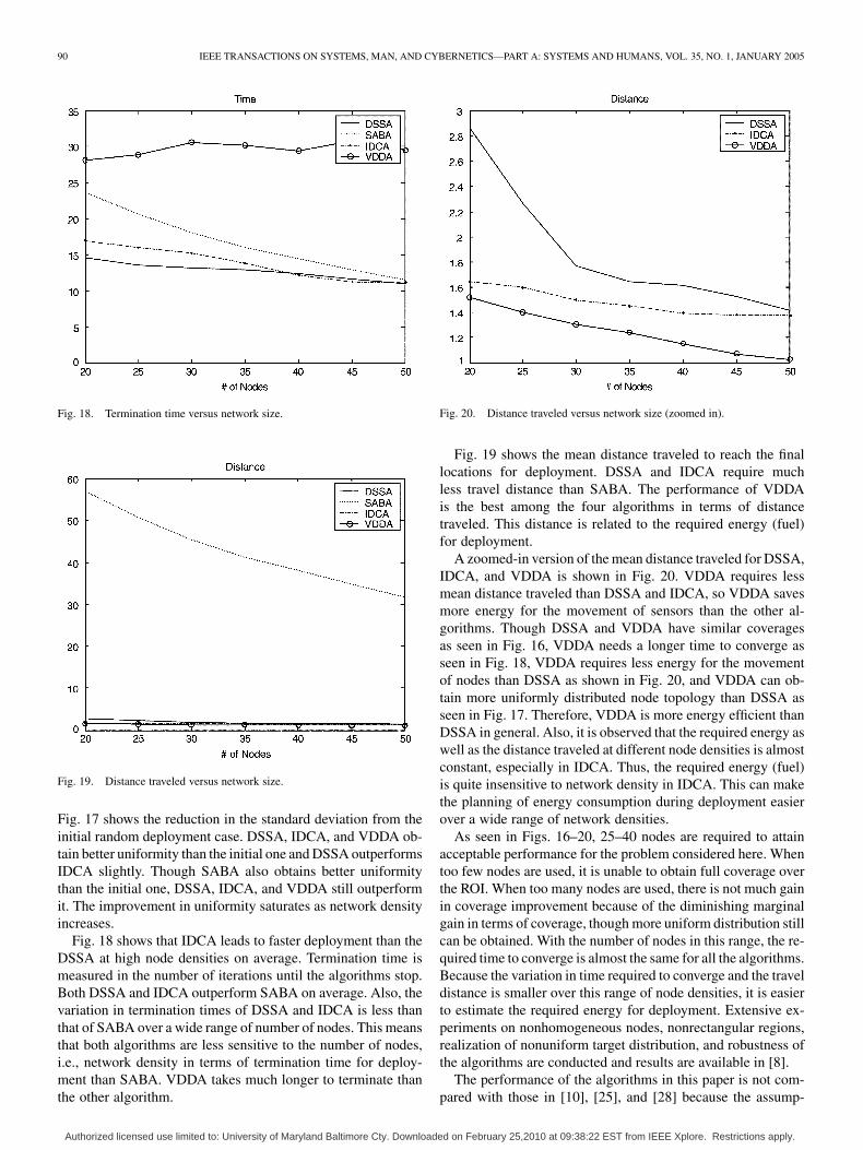
Fig. 18 shows that IDCA leads to faster deployment than theDSSA at high node densities on average. Termination time ismeasured in the number of iterations until the algorithms stop.Both DSSA and IDCA outperform SABA on average. Also, thevariation in termination times of DSSA and IDCA is less thanthat of SABA over a wide range of number of nodes. This meansthat both algorithms are less sensitive to the number of nodes,i.e., network density in terms of termination time for deploy-ment than SABA. VDDA takes much longer to terminate thanthe other algorithm.

Fig. 20. Distance traveled versus network size (zoomed in).

Fig. 19 shows the mean distance traveled to reach the finallocations for deployment. DSSA and IDCA require muchless travel distance than SABA. The performance of VDDAis the best among the four algorithms in terms of distancetraveled. This distance is related to the required energy (fuel)for deployment.

A zoomed-in version of the mean distance traveled for DSSA,IDCA, and VDDA is shown in Fig. 20. VDDA requires lessmean distance traveled than DSSA and IDCA, so VDDA savesmore energy for the movement of sensors than the other al-gorithms. Though DSSA and VDDA have similar coveragesas seen in Fig. 16, VDDA needs a longer time to converge asseen in Fig. 18, VDDA requires less energy for the movementof nodes than DSSA as shown in Fig. 20, and VDDA can ob-tain more uniformly distributed node topology than DSSA asseen in Fig. 17. Therefore, VDDA is more energy efficient thanDSSA in general. Also, it is observed that the required energy aswell as the distance traveled at different node densities is almostconstant, especially in IDCA. Thus, the required energy (fuel)is quite insensitive to network density in IDCA. This can makethe planning of energy consumption during deployment easierover a wide range of network densities.

As seen in Figs. 16–20, 25–40 nodes are required to attainacceptable performance for the problem considered here. Whentoo few nodes are used, it is unable to obtain full coverage overthe ROI. When too many nodes are used, there is not much gainin coverage improvement because of the diminishing marginalgain in terms of coverage, though more uniform distribution stillcan be obtained. With the number of nodes in this range, the re-quired time to converge is almost the same for all the algorithms.Because the variation in time required to converge and the traveldistance is smaller over this range of node densities, it is easierto estimate the required energy for deployment. Extensive ex-periments on nonhomogeneous nodes, nonrectangular regions,realization of nonuniform target distribution, and robustness ofthe algorithms are conducted and results are available in [8].

The performance of the algorithms in this paper is not com-pared with those in [10], [25], and [28] because the assump-



tions are different. In [10], additional equipment is used to de-tect other nodes and obstacles. Moreover, nodes are initially de-ployed over a compact region and then are spread out. In [25],it is assumed that there are insufficient robots in a physicallybounded region. In [28], it is assumed that global informationregarding other nodes is available.

Experiments using different values for sR and cR were con-ducted and similar performances are observed. The algorithmswere simulated in environments that are not rectangular and theperformances are similar to those of rectangular regions. Theseresults are not included in this paper due to length considera-tions. Results are available in [8].

VI. SUMMARY

The deployment problem for mobile WSN is considered inthis paper. A ROI needs to be covered by a given number ofnodes with limited sensing and cR. A random distribution ofnodes over the ROI is assumed as the initial node distribution.Though many scenarios adopt random deployment for practicalreasons, such as deployment cost and time, random deploy-ment may not provide a uniform distribution, which is desir-able for a longer system lifetime over the ROI. In this paper, anumber of distributed algorithms for the deployment of mobilenodes are proposed to improve an irregular initial deploymentof nodes. A peer-to-peer algorithm analogous to the equilib-rium of molecules and an enhanced intelligent energy-efficientdeployment algorithm for cluster-based WSN by a synergisticcombination of cluster structuring and peer-to-peer deploymentscheme are proposed. A distributed algorithm using VDs basedon local computation is also proposed. After employing thesealgorithms, the ROI is covered by more uniformly distributednodes. While developing these algorithms, one should considerfactors such as density of nodes, memory constraints, local-ization errors, and scalability of mobile nodes (network size).Through mobility and locationing ability of nodes, these algo-rithms provide a way to avoid expensive redeployment process.This postdeployment idea is quite useful for many situations, es-pecially when a large fraction of nodes are destroyed or brokenduring deployment or operation in a hostile situation, or whereinitial distribution is quite uneven and when human interventionfor redeployment is too costly or too risky. The performance ofthese algorithms is determined by the percentage of region cov-ered, computational/deployment time, the mean distance trav-eled required for deployment, and uniformity of the networks.Simulation results show that the proposed algorithms success-fully obtain a more uniform distribution from initial uneven dis-tributions in an energy-efficient manner.

In this paper, only one-hop neighbors were included whilemaking the decision regarding next nodal movement. However,better solutions in terms of energy efficiency may be found whena wider neighborhood is used. Computation cost, time delay,energy consumption, and tradeoffs between them for differentneighborhood sizes will be the main issues to be consideredin this direction. This will require the inclusion of multihopneighbors. Also, the relation between cluster-size and neighbor-hood size will need to be established for energy saving duringdeployment.

In practice, a WSN is deployed over large regions. The ROIcan be divided into multiple sub-ROIs for easy deployment, or-ganization, and management. Hierarchical deployment schemesmay be investigated to handle the scalability issue in WSNs. Thedetermination of the size of sub-ROI and their correspondingdensity and edge effects due to the division of the ROI are worthpursuing. The effect of uncertainty in sensor-node locations onthe performance of our algorithms is another area for furtherinvestigation.

REFERENCES

[1] F. Aurenhammer, “Voronoi diagrams—A survey of a fundamentalgeometric data structure,” in ACM Comput. Survey, vol. 23, 1991, pp.345–405.

[2] E. Biagioni and G. Sasaki, “Wireless sensor placement for reliable andefficient data collection,” in Proc. Hawaii Int. Conf. Syst. Sci., Jan. 2003,p. 127b.

[3] N. Bulusu, J. Heidemann, and D. Estrin, “Adaptive beacon placement,”in Proc. 21st Int. Conf. Distributed Comput. Syst., Apr. 2001, pp.489–498.

[4] , “GPS-less low-cost outdoor localization for very small devices,”IEEE Pers. Commun., vol. 7, no. 5, pp. 28–34, Oct. 2000.

[5] Y. U. Cao, A. Fukunaga, and A. Kahng, “Cooperative mobile robotics:Antecedents and directions,” Autonomous Robots, vol. 4, pp. 1–23, 1997.

[6] S. S. Dhillon and K. Chakrabarty, “Sensor placement for effective cov-erage and surveillance in distributed sensor networks,” in Proc. IEEEWireless Commun. Netw. Conf., 2003, pp. 1609–1614.

[7] D. W. Gage, “Command control for many-robot systems,” presented atthe 19th Annu. AUVS Tech. Symp, Huntsville, AL, June 22–24, 1992.

[8] N. Heo, “Distributed deployment algorithms for mobile wireless sensornetworks,” Ph.D. dissertation, Dept. Elect. Eng. Comput. Sci., SyracuseUniv., Syracuse, NY, 2004.

[9] A. Howard, M. J. Mataric, and G. S. Sukhatme, “An incremental self-de-ployment algorithm for mobile sensor networks,” Autonomous Robots,vol. 13, no. 2, pp. 113–126, 2002.

[10] A. Howard, M. J. Mataric, and G. S. Sukhatme, “Mobile sensor networkdeployment using potential fields: A distributed, scalable solution to thearea coverage problem,” in Proc. 6th Int. Conf. Distributed AutonomousRobotic Syst., Fukuoka, Japan, 2002, pp. 299–308.

[11] C. E. Jones, K. M. Sivalingam, P. Agrawal, and J. C. Chen, “A surveyof energy efficient network protocols for wireless networks,” WirelessNetw., vol. 7, no. 4, pp. 343–358, 2001.

[12] V. Kawadia and P. R. Kumar, “Power control and clustering in ad hocnetworks,” in Proc. IEEE INFOCOM Conf., 2003, pp. 459–469.

[13] S. Kirkpatrick, C. D. Gelatt, and M. P. Vecchi, “Optimization by simu-lated annealing,” Science, vol. 220, pp. 671–680, 1983.

[14] S. Kumar, F. Zhao, and D. Shepherd, “Collaborative signal and informa-tion processing in microsensor networks,” IEEE Signal Process. Mag.,vol. 19, no. 2, pp. 13–14, Mar. 2002.

[15] C. R. Lin and M. Gerla, “Adaptive clustering for mobile wirelessnetworks,” IEEE Journal on Sel. Areas Commun., vol. 15, no. 7, pp.1265–1275, Sep. 1997.

[16] L. Loo, E. Lin, M. Kam, and P. K. Varshney, “Cooperative multi-agentconstellation formation under sensing and communication constraints,”in Cooperative Control and Optimization. Norwell, MA: Kluwer,2002, pp. 143–170.

[17] S. Meguerdichian, F. Koushanfar, M. Potkonjak, and M. Srivastava,“Coverage problems in wireless ad hoc sensor networks,” in Proc. IEEEINFOCOM Conf., 2001, pp. 1380–1387.

[18] R. Min et al., “Energy-centric enabling technologies for wireless sensornetworks,” IEEE Wireless Commun., vol. 9, no. 4, pp. 28–39, Aug. 2002.

[19] J. O’Rourke, Art Gallery Theorem and Algorithms. New York, NY:Oxford University Press, 1987.

[20] G. J. Pottie and W. J. Kaiser, “Embedding the internet: Wireless inte-grated network sensors,” Commun. ACM, vol. 43, no. 5, pp. 51–58, 2000.

[21] H. Qi, S. S. Iyengar, and K. Chakrabarty, “Distributed sensor fusion-areview of recent research,” J. Franklin Inst., vol. 338, pp. 655–668, 2001.

[22] L. Schwiebert, S. K. S. Gupta, and J. Weinmann, “Research challengesin wireless networks of biomedical sensors,” in Proc. ACM/IEEE Conf.Mobile Comput. Netw., 2001, pp. 151–165.

[23] S. Slijepcevic and M. Potkonjak, “Power efficient organization of wire-less sensor networks,” in Proc. IEEE Int. Conf. Commun., vol. 2, 2001,pp. 472–476.



[24] K. Sohrabi, B. Manriquez, and G. Pottie, “Near-ground widebandchannel measurements,” in Proc. 49th Veh. Technol. Conf., 1999, pp.571–574.

[25] A. F. T. Winfield, “Distributed sensing and data collection via brokenad hoc wireless connected networks of mobile robots,” in DistributedAutonomous Robotic Systems 4, L. E. Parker, G. Bekey, and J. Barhen,Eds. New York: Springer-Verlag, 2000, pp. 273–282.

[26] Y. Xu, J. Heidemann, and D. Estrin, “Geography-informed energy con-servation for ad hoc routing,” in Proc. ACM/IEEE Int. Conf. MobileComput. Netw., July 2001, pp. 70–84.

[27] W. Ye, J. Heidemann, and D. Estrin, “An energy-efficient MAC protocolfor wireless sensor networks,” in Proc. IEEE INFOCOM Conf., vol. 3,2002, pp. 1567–1576.

[28] Y. Zou and K. Chakrabarty, “Sensor deployment and target localizationbased on virtual forces,” in Proc. IEEE INFOCOM Conf., vol. 2, 2003,pp. 1293–1303.

[29] Voronoi [Online]. Available: http://www.voronoi.com/[30] J. E. Wieselthier, G. D. Nguyen, and A. Ephremides, “Algorithms for

energy-efficient multicasting in static ad hoc wireless networks,” MobileNetw. Applicat., vol. 6, no. 3, pp. 251–263, 2001.

[31] D. W. Gage, “Command control for many-robot systems,” UnmannedSyst. Mag., vol. 10, no. 4, pp. 28–34, 1992.

Nojeong Heo received the B.S. degree in electricalengineering from Seoul National University, Seoul,Korea, in 1996 and the M.S. and Ph.D. degrees inelectrical engineering from Syracuse University,Syracuse, NY, in 1999 and 2004, respectively.

He is currently a Senior Engineer at SamsungElectronics Co., Ltd. His research interests includewireless communication, ad hoc networks, sensornetworks, and next-generation mobile networks.

Pramod K. Varshney (S’72–M’77–SM’82–F’97)was born in Allahabad, India, on July 1, 1952. Hereceived the B.S. degree in electrical engineering andcomputer science (with highest honors) and the M.S.and Ph.D. degrees in electrical engineering from theUniversity of Illinois, Urbana, in 1972, 1974, and1976, respectively.

He is currently Research Director of The NewYork State Center for Advanced Technology inComputer Applications and Software Engineering(CASE). During 1972–1976, he held teaching and

research assistantships at the University of Illinois. Since 1976, he has beenwith the Department of Electrical and Computer Engineering, SyracuseUniversity, Syracuse, NY, where he is currently Professor of electrical engi-neering and computer science. He has served as the Associate Chairman of thedepartment from 1993 to 1996. His current research interests are in distributedsensor networks and data fusion, detection and estimation theory, wirelesscommunications, image processing, remote sensing, radar signal processing,and parallel algorithms. He has supervised 34 Ph.D. dissertations, authored orcoauthored over 85 journal papers and over 250 conference papers. He is theauthor of Distributed Detection and Data Fusion (New York: Springer-Verlag,1997). He has consulted for General Electric, Hughes, Booz-Allen andHamilton, SCEEE, Kaman Sciences Corp., Andro Computing Solutions, ITT,and Digicomp Research.

Dr. Varshney is a member of Tau Beta Pi and is the recipient of the 1981 ASEEDow Outstanding Young Faculty Award. He was elected to the grade of Fellowof the IEEE in 1997 for his contributions in the area of distributed detection anddata fusion. In 2000, he received the Third Millennium Medal from the IEEEand Chancellor’s Citation for Exceptional Academic Achievement at SyracuseUniversity. He was the Guest Editor of the Special Issue on Data Fusion of thePROCEEDINGS OF THE IEEE, January 1997. He is on the editorial board of ClusterComputing Information Fusion. He is a Distinguished Lecturer for the IEEEAES Society. He was the President of the International Society of InformationFusion in 2001. While at the University of Illinois, he was a James Scholar, aBronze Tablet Senior, and a Fellow.


Energy-Efficient Deployment of Intelligent Mobile Sensor Networks

Documents

Transcript of Energy-Efficient Deployment of Intelligent Mobile Sensor Networks