Energy-e cient Localization Via Personal Mobility Pro...

Energy-efficient Localization Via PersonalMobility Profiling

Ionut Constandache1, Shravan Gaonkar2, Matt Sayler1,Romit Roy Choudhury1, and Landon Cox1

1 Duke University, Durham, NC, USA,{ionut,sayler,lpcox}@cs.duke.edu,[email protected],

2 University of Illinois at Urbana Champaign, IL, [email protected]

Abstract. Location based services are on the rise, many of which as-sume GPS based localization. Unfortunately, GPS incurs an unaccept-able energy cost that can reduce the phone’s battery life to less thanten hours. Alternate localization technology, based on WiFi or GSM,improve battery life at the expense of localization accuracy. This paperquantifies this important tradeoff that underlies a wide range of emerg-ing applications. To address this tradeoff, we show that humans canbe profiled based on their mobility patterns, and such profiles can beeffective for location prediction. Prediction reduces the energy consump-tion due to continuous localization. Driven by measurements from NokiaN95 phones, we develop an energy-efficient localization framework calledEnLoc. Evaluation on real user traces demonstrates the possibility ofachieving good localization accuracy for a realistic energy budget.

1 Introduction

Mobile phones are becoming a powerful platform for sensing, sharing, and query-ing people-centric information. A variety of applications are on the rise, manyof which utilize location to express the context of information. Examples includegeotagging, geocasting, asset tracking, context-aware search, location-specific ad-vertisements, and visualization [1, 2, 3]. Most of these location based applications(LBAs) assume GPS capabilities. While GPS offers good location accuracy ofaround 10m, it incurs a serious energy cost that can drain a fully charged phonebattery in 8.5 hours [1]. We make a few observations in light of this energy-accuracy profile.

1. In real life, the phone battery must be shared with several other needs, in-cluding voice calls, emails, pictures, SMS, and an emergency reserve. The en-ergy budget available for localization alone is a small fraction of the batterycapacity. If this fraction is assumed to be 25%, continuous GPS localizationwill sustain for less than 2.5 hours.

2. One may argue that continuous GPS localization is not necessary – GPScan be activated only on demand. While this may suffice for some services

2 Ionut Constandache et al.

(such as geo-tagging a photo), a large number of emerging applications aredemanding frequent location updates from users. For example, GeoLife [4]plans to track a phone and display shopping lists when the phone-user is neara grocery store. Micro-Blog [1] proposes to query users in a desired regionfor participatory sensing applications [3]. TrafficSense [5], Pothole Patrol [6]and Nericell [7] require phones to continuously report accelerometer readingsto better estimate traffic/road conditions. All these applications rely on thefeasibility of continuous localization over reasonably long time scales.

3. Continuous localization over long time scales results in higher average error.Given an energy budget of K GPS readings, and a duration of T > K timeunits, (T − K) time units cannot be assigned location readings. Locationscan only be estimated at these unassigned times, and hence, are likely to bemore erroneous than actual GPS readings. When averaged over all actualand estimated readings, the average localization error proves to be higherthan the instantaneous error (around 10m for GPS). As the energy budgetdecreases, the difference between average and instantaneous error increases.

4. Alternate WiFi and GSM based localizations are not obvious replacementsto GPS. While these schemes are less energy-hungry, they incur higher (in-stantaneous) localization error (around 40m and 400m respectively). Thispermits greater number of location readings, each of which is less accurate.Whether this results in lower average error than that of a few, but accu-rate, GPS readings, is an open question. Whether an optimal combinationof GSP/WiFi/GSM based localization meets application-demands, is also anunexplored research direction.

This paper investigates the space of energy-efficient localization for mobilephones. We quantify the energy-accuracy tradeoff through measurements onNokia N95 phones. We formulate a theoretical framework using dynamic pro-gramming (DP), that derives the optimal localization accuracy under a givenenergy budget. When results show that the theoretical optimal with basicGPS/WiFi/GSM technologies may not suffice for high-accuracy applications,we explore usefulness of predictions. Habitual movements of humans, and theirsimilarity to statistical behavior of large populations, are potential opportuni-ties. We incorporate predictions in our offline DP and design online heuristics foruse on mobile phones. Performance results, comparing the optimal to the onlineheuristics, confirm the feasibility of achieving localization in the order of 25m,over a day’s energy budget. Certain limitations will have to be addressed beforeour proposed system, EnLoc, can be deployed for public use – we discuss theselimitations, and indicate directions of future work. Our main contributions canbe summarized as follows.

Identifying the space of energy-accuracy tradeoff. We quantify thetradeoff with measurements on Nokia N95 phones.

Energy-efficient Localization Via Personal Mobility Profiling 3

Analysis of the optimal localization accuracy for a given energybudget. For a given mobility trace, an offline dynamic program computesthe maximum accuracy achievable through GPS, WiFi, GSM, or combinationsthereof.

Exploiting habitual activity of individuals, and behavior of popula-tions, to predict location. Predictions incorporated into the DP offer optimalsolutions. Online heuristics permit energy-efficient localization in real time.

Evaluation of heuristics in real life situations. A wireless map of theUIUC campus is created through war-driving, and real mobility traces derivedfrom student phones. Performance of heuristics is compared with the optimalusing a custom trace-based simulator.

The rest of the paper expands on each of the contributions.

2 Motivation

We used the Nokia Energy Profiler [8] to measure fine-grained power consump-tion in Nokia N95 phones. With this monitor running in the background, weperformed GPS, WiFi, and GSM based localization. This section reports the re-sults recorded, and highlights key observations that motivate EnLoc. However,we first provide a brief background on WiFi and GSM localization techniques,originally proposed in [9].

Localization Using WiFi and GSMAs a benchmark, we measured localization error with on-phone GPS hardware,and found an average accuracy of 10m in clear-sky, outdoor conditions. GPSwas mostly unavailable indoors. To circumvent GPS hardware and its problemsindoors, project Place Lab [9, 10] proposed interesting alternates to GPS local-ization. Specifically, authors create a wireless map of a region by war-driving inthe area. The wireless map is composed of sampled GPS locations, WiFi accesspoints and GSM towers audible at these locations, and their corresponding signalstrengths. This wireless map is then distributed to phones. When a phone trav-els through the mapped area, it estimates its own location by matching its listof audible WiFi APs to the wireless map. Several matching schemes have beenproposed, including Centroid Computation, Signal Strength based estimation,and Fingerprinting. Place Lab experiments in Seattle region exhibit a medianpositioning error of 13 to 40m with WiFi, and around 94 to 196m with GSM.When performed in Champaign, IL, and Durham, NC, the errors were higher.Specifically, WiFi accuracy ranged between 25 to 40m, while GSM ranged be-tween 300 to 400m. The increase in GSM error was due to a smaller number ofcells and using a single GSM provider.


Fig. 1. Power consumption in mW: (a) GPS localization every 30 seconds. (b) GPSperiodically turned off. (c) WiFi localization every 30 seconds. (d) GSM localizationevery 30 seconds.

Energy Measurements for GPS, WiFi, and GSMWe measured the energy consumption on Nokia N95 phones for each localizationscheme. For this, we charged the phone to its full battery capacity, and turnedoff all applications and communication technologies. Then, we invoked the en-ergy monitoring program and turned on only the location sensor we aimed tomeasure. Our program probed the location sensor at a chosen interval, Tprobe,that varied from 30 to 300 seconds.

Figure 1(a) shows GPS power consumptions as a function of time, for Tprobe

= 30 seconds. We see periodic spikes on top of a baseline power consumptionat approximately 400 mW. The spikes correspond to the periodic probes whichtrigger a sensor read and a data write operation into the phone’s file system.The baseline corresponds to the power consumed by the GPS receiver. To provethis, we periodically turned off all sensors, including GPS. Results in Figure1(b) show a baseline power consumption of around 55 mW when all sensors areturned off.

Similar measurements for WiFi and GSM are reported in Figure 1(c) and (d).Observe that while the baseline power consumption for WiFi is low (55 mW),


it exhibits a high spike (of around 1300 mW) at every probe. GSM based sam-ples also exhibit similar characteristics, however, their power consumption is less.

Based on these power measurements, we computed the total battery lifetimefor each sensor as if the entire battery capacity is used for localization alone.The results are presented in table 1 together with the localization accuracy ofeach sensor. We record battery lifetimes of around 10, 40, and 60 hours, for GPS,WiFi and GSM, respectively. When viewed against corresponding localizationaccuracies of 10, 40, and 400 meters, the energy-accuracy tradeoff is evident.

Sensor GPS WiFi GSM

Lifetime (h) 10 40 60

Loc. error (m) 10 40 400

Table 1. Energy-Accuracy Tradeoff

3 EnLoc: Framework Design

3.1 Average Location Error (ALE)

The energy-efficient localization problem can be defined as follows. Given anenergy budget EB , time duration T , and a set of localization schemes S, designa strategy that will minimize the average localization error over the entire time,T . Formally, denote Lreported(ti) and Lactual(ti) to be the reported and actuallocations of the phone at time ti. Assuming T discrete time-points in the entiretime duration, the average localization error δavg, is defined as

δavg =T∑

i=1

(Lreported(ti)− Lactual(ti)T

)where Lreported(ti)−Lactual(ti) is the distance between the reported location

and the actual location at time ti.

Assuming GPS to be the ground truth, a GPS reading at time tj impliesthat Lreported(tj) is same as Lactual(tj). Similarly, a WiFi reading at tj impliesthat Lreported(tj) − Lactual(tj) is in the order of 40m. The problem then is tominimize δavg for a given energy budget. We model this energy-accuracy tradeoffas an optimization problem.

3.2 Problem Formulation

Our goal is to determine a schedule with which the location sensors should betriggered such that the ALE is minimized under a given energy budget. We


Fig. 2. Error vs time model of physical movement.

envision a schedule to be a set of time instants, {t1, t2, t3, ..}, and correspond-ing sensors {s1, s2, s3, ..}, where si ∈ [GPS,WiFi,GSM ]. The optimal scheduletriggers a reading of sensor si at time ti to minimize ALE. We elaborate withan example.

Consider the case in which a person begins moving at time t0, from an ini-tially sampled location, L(t0). Assume that until the next location reading, thislocation is periodically reported as the location of the phone. As the personmoves away from the original location, the location error increases with time.When the person stops moving, the error remains static; when the person movestowards the L(t0), the error starts decreasing. Without loss of generalization,Figure 2(a) and (b) show an example trajectory in discrete time, and the cor-responding error versus time graph. The phone moves away for 2 time steps,pauses for 2 time steps, moves further away for another two time steps, andthen pauses again for one time step. The total error due to this movement canbe computed as the sum of the 7 vertical lines, dropped from the error curve tothe x axis. For easier explanation, let us assume this is the area under the curve.

Now, if the user takes a GPS reading at time t4, the corresponding error graphis shown in Figure 2(c). Time t4 onwards, the error increases as if location L(t4) isthe new (known) starting location. If no other readings are taken, the reduction


in total error due to the GPS reading is the shaded area labeled “Accuracy gainfrom GPS”. If a WiFi reading is scheduled at time t6, the instantaneous error,unlike GPS, does not reach zero – this results in error reduction shown by thediagonally striped rectangle. In general, the reduction depends on the time-pointat which the reading is taken, as well as the sensor used. Additional locationreadings at subsequent time-points offer further error reductions, at the cost ofexpended energy. Hence, the problem of energy-efficient localization translatesto finding the appropriate time-points and sensors that must be scheduled tominimize the localization error. More formally, for a given energy budget, EB ,energy consumption per-sensor, esi , and a mobility trace, τ , the algorithm mustproduce a < timei, sensori > schedule, that minimizes the total area under theerror curve. We approach this problem using dynamic programming. Relatedproblems in the context of satellite communication and user state recognitionhave been investigated in [11] and [12].

3.3 Dynamic Programming

The dynamic program computes the minimum error accumulated till the endof a given trace, and the corresponding < ti, si > schedule that achieves it.For this, the accumulated error is expressed as a sum of (1) error accumulateduntil some time j when the last location reading was taken, and (2) error ac-cumulated from j till the final time instant, T . Now, any accumulated errorbetween two consecutive location readings at time i and j can be computed as∑j−1

k=i+1(Lreported(k)−Lactual(k)), where Lreported(k)−Lactual(k) is the distancebetween the estimated/reported location, and the actual location. Without lossof generality, assume that Lreported returns the last known location. Thus, theaccumulated error between i and j is

∑j−1k=i+1(Lactual(i)−Lactual(k)). Since this

accumulated error is a function of the sensor used at i (recall Figure 2), we definethree matrices EGPS [i][j], EGSM [i][j], EWiFi[i][j]. Each matrix corresponds tothe localization sensor in the subscript, and denotes the total error from i to j,when that sensor is used at time i. The last column of these matrices gives usthe error from some last reading at time j till the end of the trace at time T .Table 2 presents the notations used in the dynamic program.

For the first term, we need to minimize the accumulated error till the (last)reading at time j. This problem can in turn be formulated as finding a secondlast reading, say at time i, which minimizes the error until j. This can be re-peated under the constraints of a maximum number of feasible readings.

Let us consider the problem of finding the minimum error accumulated tilltime j, assuming a GPS reading is executed at j. There must exist a previoustime i < j, at which the previous reading was taken. At time i, any one of GPS,WiFi or GSM sensors could have been used. Since there is no other readingbetween i and j, some error accumulates from i to j. This accumulated error isone of EGPS [i][j], EWiFi[i][j] or EGSM [i][j], depending on the location sensor


Notation Explanation

T Trace length in time units

IWiFi[j], Instantaneous error at time unit j when the WiFi/GSMIGSM [j] sensor is used.

EGPS [i][j], Accumulated error between i and j or sum ofEWiFi[i][j], instantaneous errors at intermediate time units, if at iEGSM [i][j] GPS/WiFi/GSM sensor was used and until j there is

no other reading.

minGPS [i][n1][n2][n3], Minimum accumulated error till time unit i, if i was theminWiFi[i][n1][n2][n3], last scheduled reading and used the GPS/WiFi/GSMminGSM [i][n1][n2][n3] sensor. The minimum is achieved with n1 GPS, n2 WiFi

and n3 GSM readings.

totalErrorGPS [j][n1][n2][n3] Total accumulated error till the end of the trace if attotalErrorWiFi[j][n1][n2][n3] time unit j the GPS/WiFi/GSM sensor was used andtotalErrorGSM [j][n1][n2][n3] there are no further readings till the end of the trace.

In total there are n1 GPS, n2 WiFi, n3 GSM readings

Table 2. Summary of notation.

used at time i. The problem of finding the minimum error till time j translatesinto solving the minimum sum of two terms – (i) the minimum accumulated errortill some time i < j using some sensor (GPS,WiFi or GSM), and (ii) the erroraccumulated between i and j. However, the minimum accumulated error till timei has 1 GPS reading less (because one GPS reading is invested in estimating thelocation at time j). Since, there are three possible sensors that can be used attime i, the optimization can be formulated as:

minGPS [j][n1][n2][n3] = mini

minGPS [i][n1− 1][n2][n3] + EGPS [i][j],minWiFi[i][n1− 1][n2][n3] + EWiFi[i][j],minGSM [i][n1− 1][n2][n3] + EGSM [i][j]

where j > i, j >= n1 + n2 + n3, T > j.

The total error till the end of the trace (if the last reading is at time j), isthe minimum error achieved till j plus the accumulated error between j and T .

totalErrorGPS [j][n1][n2][n3] = minGPS [j][n1][n2][n3] + EGPS [j][T ]

Similarly, we can write the above equations for the case in which WiFi orGSM is used for reading the location at time j. However, we must add an ad-ditional term to denote the instantaneous location error at time j (recall thatWiFi and GSM sensors have an instantaneous error represented as IWiFi[j] andIGSM [j]). The dynamic program for a WiFi reading at time j is

minWiFi[j][n1][n2][n3] =

mini

minGPS [i][n1][n2− 1][n3] + EGPS [i][j] + IWiFi[j],minWiFi[i][n1][n2− 1][n3] + EWiFi[i][j] + IWiFi[j],minGSM [i][n1][n2− 1][n3] + EGSM [i][j] + IWiFi[j]


and that for a GSM reading at j is

minGSM [j][n1][n2][n3] =

mini

minGPS [i][n1][n2][n3− 1] + EGPS [i][j] + IGSM [j],minWiFi[i][n1][n2][n3− 1] + EWiFi[i][j] + IGSM [j]minGSM [i][n1][n2][n3− 1] + EGSM [i][j] + IGSM [j]

The total error till the end of the trace, if the last reading at time unit j usesthe WiFi sensor, is:

totalErrorWiFi[j][n1][n2][n3] = minWiFi[j][n1][n2][n3] + EWiFi[j][T ]

while for the GSM sensor, total error can be expressed as:

totalErrorGSM [j][n1][n2][n3] = minGSM [j][n1][n2][n3] + EGSM [j][T ]

The final solution for the minimum accumulated error till the end of thetrace, given a maximum of n1 GPS readings, n2 WiFi readings and n3 GSMreadings, is:

Sol = minj,n1,n2,n3

totalErrorGPS [j][n1][n2][n3]totalErrorWiFi[j][n1][n2][n3]totalErrorGSM [j][n1][n2][n3]

The< ti, si > schedule can be retrieved by keeping track of timing and sensorreadings for each minimization sub-problem. In this way, the entire solutionsequence can be retrieved and the optimal schedule computed.

3.4 Optimal Localization Error

To obtain the best localization accuracy, we executed the DP on mobility tracesfrom the UIUC campus. We first war-drove the campus [9] and generated a wire-less map of the area (as described in Section 2). Then, we distributed phonesto students to gather mobility traces. A custom simulator integrated the traceswith the wireless map, and executed the dynamic program. We briefly present afew relevant details.

Collecting Mobility TracesOur tracing software (installed on mobile phones) sampled the GPS location,as well as the WiFi and GSM base station IDs every 30 seconds. For purposesof anonymity, we requested the users to turn off their mobile phones when theydid not wish to be tracked. The traces were analyzed offline. For each sample,the set of WiFi APs were obtained and the corresponding locations extractedfrom the (war-driven) wireless map. A centroid of all the WiFi AP locationswas computed and declared to be the instantaneous WiFi-based location of thephone. Since the GPS location for this time instant is known, the instantaneouserror from WiFi localization can be computed. This instantaneous error (say


at time, ti) populates the IWiFi[i] value in the dynamic program formulation.The GSM localization error is identically computed, and used to populate theIGSM [.] matrix. In summary, for a given mobility trace, the exact errors due toWiFi and GSM localization is known for each time instance1. These errors arefed into the DP for error computation. The energy budget is specified as 25% ofthe phone battery, while the required duration of operation is 24 hours.

We evaluate four schemes, namely, Optimal GPS, Optimal WiFi, OptimalGSM, and Optimal Combined. As the name suggests, Optimal GPS correspondsto the minimum average localization error achieved when only GPS readings areused. In the interest of space, Table 3 reports results from three representativemobility traces. Observe that Opt WiFi outperforms Opt GPS indicating thatgreater number of less accurate readings is better for mobile phone localization.Also, Opt Combined outperforms the others, and is close to Opt WiFi in manyof the traces. However, it is surprising that even the offline optimal error (withknowledge of the entire trace) was typically more than 60m. Online versions ofthese schemes, that do not have the entire trace, will naturally perform worse.This warrants enrichments that would improve the limits of energy-constrainedlocalization. We observe that “reporting the last known location between loca-tion readings” is a source of inefficiency, and seek solutions that exploit mobilityprediction.

OptGPS OptWiFi OptGSM OptComb

Trace 1 164.999 78.52 352.909 78.52

Trace 2 105.35 75.16 327.116 58.66

Trace 3 125.848 62.134 370.621 62.134

Table 3. Optimal performance for different traces

3.5 Prediction Opportunity

The error model discussed thus far assumes that between two successive locationreadings, L(ti) and L(tj), the location reported is the last known location, L(ti).In reality, human behavior/mobility is amenable to prediction [13, 14, 15, 16].Driving on straight highways, turns on one way streets, habitual office hours, areexamples of prediction opportunities. EnLoc aims to take advantage of them.

Simple Linear Predictor: We begin by considering a basic linear predictor.The location of a phone at time tk, denoted L(tk), can be a linear extrapolationof the two previously sampled locations, L(ti) and L(tj). This can be effectivewhen a phone moves on a straight road. However, if the phone’s movement isnot straight, or if L(ti) and L(tj) were highly erroneous, linear prediction maybe unsuitable. Therefore, the performance of linear predictors may not be con-sistent, and needs evaluation. We have modified the DP to incorporate linearprediction; we omit the formal details in the interest of space.

1 We assume that GPS is the ground truth.


Human Mobility Patterns: While linear prediction is a generalized ap-proach, capturing individual human behavior may facilitate better predictions[14, 15]. The intuition is that humans have habitual activity patterns, and sam-pling the activity at a few uncertainty points may be sufficient for predicting therest. For instance, given that a person goes to lunch at either 12:00pm, 12:50pm,or 1:00pm, the phone may trigger GPS readings just after these times. Learn-ing that the person has started out for lunch, her subsequent locations can bepredicted (i.e., locations along the habitual path from office to the cafe). In thenext section, we augment EnLoc with such human-tailored predictions. Prob-lems arise when the person deviates from her habitual pattern.

Deviations: To cope with deviations from habitual paths, we hypothesizethat statistical behavior of large populations provide useful hints. At a trafficintersection, knowing that most of the vehicles take a left turn can be valuablefor prediction. In general, if a “ probability map” can be generated for a givenarea, an individual’s mobility in that area can be partially predicted. We describethe design of such a probability map later. However, assuming we have such aprobability map, we are able to extend our DP to extract the optimal localizationschedule for a given trace. Intuitively, the DP is expected to schedule locationreadings at points where the individual’s actions disagree with the populationbehavior. Where the behavior agrees with the majority of the population, theDP can save energy.

4 EnLoc: System Solution

This section describes a complete system solution, EnLoc, for performing energy-efficient localization on mobile phones. The solution exploits both habitual mo-bility patterns and population-driven probability maps. EnLoc is an online so-lution, and unlike the DP, does not assume knowledge of the user’s entire trace.Results presented in Section 5 compare EnLoc with the offline optimal schemes.

Exploiting Habitual MobilityA study with 100, 000 people has shown that individuals exhibit habitual space-time movements, with reasonably small variation [13]. If designed carefully, afew location samples may be sufficient to track the location/movement of theperson over long time scales. To understand this better, we collected GPS-basedmobility traces of several people over a month, and plotted them over GoogleMaps. Figure 3(a) shows a simplified example.

One may envision the Google maps plot as a tree, with branches at certainpoints – we call this the logical mobility tree (LMT)2. The vertices of this tree

2 We are aware that the traces can very well form a graph, however, envisioning thisas a tree facilitates easier explanation. The ideas we propose are general to logicalmobility graphs.


Fig. 3. (a) An anonymous user’s movements over two weeks. (b) A spatial logicalmobility tree. (c) A space-time logical mobility tree.

are the branching points on the person’s actual mobility paths. While trackinga phone along a path on the tree, uncertainty arises at these branching points,and hence, the nodes of the LMT are also called uncertainty points. The edges ofthe LMT represent physical traces that connect consecutive uncertainty points.Each edge is associated with (1) the starting time of that physical movement,(2) the average velocity on that path, and (3) the duration of travel on thatphysical path. Figure 3(b) shows the LMT corresponding to the physical mobil-ity in Figure 3(a).

Our key idea is to schedule location readings right after the uncertainty pointson the LMT. Such a location reading will resolve the uncertainty since the phonewill be placed in one of the paths emanating from that uncertainty point. Thus,the phone’s location can be reasonably predicted until it encounters the nextuncertainty point, at which time, another location reading will be necessary. Forinstance, a location reading at the Vine/Mich intersection can tell whether theperson is headed towards the Penn/Dom intersection, or the Vine/Wash inter-section. Of course, problems arise due to time variations.

Observe that the LMT in Figure 3(b) is a spatial representation of a person’smobility profile. In reality, a person traverses the same edge on the LMT atmany different times (e.g., one may leave for office at different times between8:00 and 9:00am). Each of these possibilities translates into a distinct edge in theLMT. Figure 3(c) shows a hand-constructed example of such a space-time LMTrepresentation. To accurately know when the phone leaves a particular node ofthe LMT, EnLoc will need to sample all the edges emanating from that node.Since a person can start moving across a large number of time points (i.e., alarge number of edges), the energy budget may not permit sampling at all thesetimes. Only a fraction of the emanating edges will need to be sampled. EnLocdesigns a heuristic to sample a subset of the edges branching out of a node.We explain this with the example of Figure 3(c), which is not derived from theactual mobility trace.


Assume that current time is 8:00am, and the phone is located at home,H. Also assume that the remaining energy budget is Bremaining. The heuris-tic begins by identifying all the paths from H to the leaves of the tree, i.e.,P1 = home ⇒ coffee, and P2 = home ⇒ walmart. Then, the number of loca-tion readings Ni, necessary to track the phone with certainty, is computed foreach path Pi. Thus N1 = 4 + 6 = 10 readings. Observe that 4 readings are nec-essary to track the phone leaving Home, and 6 readings for going from Office toCoffee. These 6 readings include the 5 edges from Office to Coffee (the latest be-ing 6:10pm), as well as the 6:00pm edge from Office to Gym. If the 6:00pm edgeis not included, EnLoc may not know if the phone has started moving towardsthe Gym. Similarly, N2 = 4 + 8 + 3 = 15 readings. Now, the heuristic computesM = max(Ni), a pessimistic estimate of the number of readings necessary in thefuture; M = 15 for this example. Then, the heuristic computes F = eH

M , whereeH is the number of emanating edges from Home. In this example, F = 4

15 . Thephone is allocated F ×Bremaining amount of energy for detecting its departurefrom home. Assuming Bremaining is 10, there are approximately 2 GPS readingsavailable. The heuristic randomly chooses 2 time-points out of the 4, and samplesthe phone’s location. Once that phone is found to be on one of the paths goingout of Home, the heuristic predicts the phone’s location based on the habitualvelocity on that edge. At the next uncertainty point, the phone recomputes Fusing the same scheme above. The overall system is reset at night when thephone is plugged into the power outlet.

Addressing Deviation from HabitsUsers may deviate from their habitual paths, and the above scheme will not beable to predict their locations. Even though deviations are not the common case,they are important because several applications may be triggered due to devi-ation. For instance, micro-blogging [1] may be more active when people go forvacations; location-specific information may be necessary when people are driv-ing down untraveled paths. EnLoc addresses the case of deviation – the mainidea is to exploit mobility of large populations as an indicator of the individ-ual’s mobility. Consider a person approaching a traffic intersection from StreetA. Since the person has not visited this street in the past, it is difficult to pre-dict how she will behave at the imminent intersection. Now, if a large fractionof the population is known to take a left turn onto Street B, then the person’smovement can be guessed accordingly. EnLoc creates, and takes advantage of,population-driven mobility maps. The details follow.

EnLoc detects a deviation when a scheduled location reading discovers thephone in an unexpected location. At this time, EnLoc switches to the Devia-tion Mode of operation. In this mode, the residual energy budget is divided intoequally spaced GPS readings across the remainder of the day. If the currenttime is 5:00pm, the remaining energy budget is 48 GPS readings, and there are6 hours left before a habitual battery recharge (say at 11:00pm), EnLoc sched-ules 8 equally spaced readings per hour. Now, once the first location sample has


Fig. 4. UIUC campus intersection with associated probability matrix

been obtained, say L(t1), EnLoc uses the population activity map to predictthe phone’s movement. The velocity is estimated from the activity map, as wellas turns at different intersections. Incorrect predictions obviously incur locationerror. The error accumulates until the next reading at time t2, at which pointEnLoc starts a new prediction using location L(t2) as the starting point. Ofcourse, this heuristic needs the population-driven activity map for a given area.We created such a map of the UIUC campus, described next.

Without loss of generalization, let us consider 4-way traffic intersections.EnLoc computes 4 probabilities for each intersection, i.e., an user entering theintersection from Street A, either turns left, turns right, continues straight, ortakes a U-turn. One may envision this as a 4×4 matrix, where element ij denotesthe probability that the user entering street i exits through street j. Our firstapproach towards creating this matrix was to deploy sound/vibration sensors attraffic intersections, and count passing vehicles through simple signal process-ing. When this proved complicated, we adopted a much simpler approach at theexpense of some inaccuracy.

On Google maps, we identified all segments of roads that border the UIUCcampus. Further, we identified roads that intersect the bordering roads, andenter the campus. We call these feeder roads. Observe that all vehicles mustenter the university campus through one of these feeder roads. We also identifiedall parking lots within the campus, their capacities, and the total number ofactive parking passes in the university. Now, we simulated vehicles that enterthe campus through a feeder road, and drives to a pre-specified parking lot. Thepre-specified parking lot is randomly chosen from the distribution of parkinglot sizes (i.e., proportionally more cars are destined to bigger lots). For eachvehicle, we obtained its driving direction through Google Maps APIs [17], andparsed it to extract the vehicle’s movement at each traffic intersection (i.e.,left/right/forward/backward). Simulations of thousands of vehicles produces theprobability matrix for each intersection. Figure 4 shows the intersections onthe UIUC campus, and a probability matrix for one of them. We expect the


probability map to be installed in phones, and thereby used for online predictionand localization.

5 Evaluation

We evaluate EnLoc using realistic traces collected from mobile phones of UIUCstudents. Traces were processed offline to extract their time durations, GPS lo-cations (every 30 seconds), as well as the WiFi APs and GSM towers overheardalong the paths. Trace segments located within the war-driven campus were pro-cessed to obtain the WiFi and GSM localization errors for every 30 second timepoints (we assume GPS is ground truth). Further, at each traffic intersection, themobility of the phone was predicted based on the maximum probability at theintersection. The error was computed whenever the prediction was inconsistentwith the actual user’s movement. All the errors were systematically incorporatedinto our custom simulator (which includes the dynamic program module). Theenergy budget for localization was assumed to be 25% of the battery capacity,while the required duration of operation was 24 hours.

An ideal evaluation of EnLoc should characterize the average localizationerror (ALE) over a person’s complete mobility pattern (i.e., habitual and de-viant paths). However, since the deviations in our traces extended far beyondthe (war-driven, probability-mapped) UIUC campus, we were unable to performan ideal evaluation. Instead, we first evaluated several trace segments confinedwithin the UIUC campus (we pretend these are the deviant paths). Then, weevaluated the habitual mobility profile-based approach by pruning the deviationsfrom a user’s LMT. We believe that in reality, the localization error will be closeto the average of these two cases.

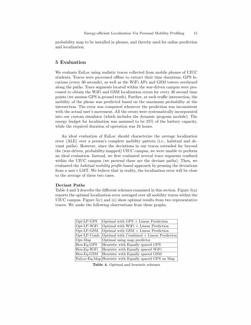
Deviant PathsTable 4 and 3 describe the different schemes examined in this section. Figure 5(a)reports the optimal localization error averaged over all mobility traces within theUIUC campus. Figure 5(c) and (e) show optimal results from two representativetraces. We make the following observations from these graphs.

Opt-LP-GPS Optimal with GPS + Linear Prediction

Opt-LP-WiFi Optimal with WiFi + Linear Prediction

Opt-LP-GSM Optimal with GSM + Linear Prediction

Opt-LP-Comb Optimal with Combined + Linear Prediction

Opt-Map Optimal using map predictor

Heu-Eq-GPS Heuristic with Equally spaced GPS

Heu-Eq-WiFi Heuristic with Equally spaced WiFi

Heu-Eq-GSM Heuristic with Equally spaced GSM

EnLoc-Eq-Map Heuristic with Equally spaced GPS on Map

Table 4. Optimal and heuristic schemes


(1) As mentioned earlier, OptWiFi consistently outperforms OptGPS. Evi-dently, this trend holds for the case of linear prediction as well. Opt-LP-WiFiaverages an error of 28.94m, in comparison to 36.06m from Opt-LP-GPS. Weconclude that, when scheduled carefully, WiFi offers better energy-efficient lo-calization than GPS/GSM.

(2) Linear prediction performs well even for mobility traces that take fre-quent turns. This may appear surprising because linear prediction is expectedto yield higher errors when an user has taken a right-angle turn. Examination ofthe optimal schedule for “manhattan type” traces offered useful insights. Whenthe distances between consecutive turns were short, the linear predictor approx-imated the movement with a straight line cutting through the trace. The erroris not large, as evident from Figure 6(a). On the contrary, if the trace has longstretches of straight lines, the Opt-LP scheme naturally predicts correctly (seeFigure 6(b)).

(3) When using probability maps, the optimal ALE proves to be small. Thisis because the number of mis-predictions (at the intersections) are typically fewerthan the number of location readings permitted by the budget. As a result, Opt-Map schedules a location reading wherever there is a mis-prediction. Of course,we assumed that the velocity of the phone can be perfectly predicted, and hence,errors arise only after mis-predictions. In reality, some errors will accumulate asa result of inaccurate velocity prediction. We plan to address this issue as a partof our future work, potentially using phone accelerometers to predict the velocity.

Figure 5(b)(d)(e) present the performance of online heuristics. Consistentwith our earlier observation, Heu-Eq-WiFi outperforms both Heu-Eq-GPS andHeu-Eq-GSM. However, EnLoc-Eq-Map outperforms Heu-Eq-WiFi, except inrare occasions (such as in Trace B). The reason is as follows. In trace B, thephone encounters a road block, and takes a detour from its natural path to-wards the destination. As a result, it takes turns that are inconsistent with themap predictions. Since this detour causes many mis-predictions, the budgetednumber of readings are not sufficient to correct them. The probability map canbe updated when there are road blocks in the neighborhood, and a phone canperiodically download a fresh copy of the map from a web service. In general,however, results indicate that heuristics based on probability maps are reason-ably effective for achieving energy-efficient localization. We are unsure if similarresults may hold for places unlike university campuses – we discuss these issuesin Section 6.

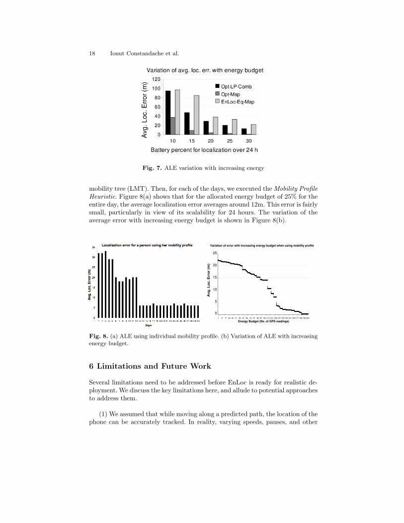
Figure 7 shows the variation of ALE (averaged over all traces) for increasingenergy budget. The error from optimal schemes decreases monotonically withincreasing energy. The EnLoc-Eq-Map scheme follows a similar trend.


Fig. 5. Average localization error using optimal schemes: (a) Optimal over all traces,(b) Heuristic over all traces, (c) Optimal on Trace A, (d) Heuristic on Trace A, (e)Optimal on Trace B, (f) Heuristic on Trace B.

Fig. 6. Linear prediction performs well on (a) Manhattan, (b) Highway movement.

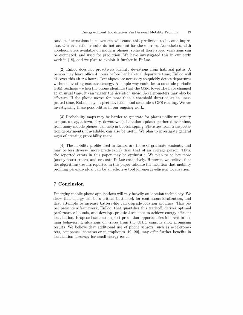
Habitual MobilityNext, we present the localization error when a person’s mobility profile is utilizedfor prediction. We use an anonymous student’s mobility profile derived from30 days of traces. We processed her mobility traces and generated the logical


Fig. 7. ALE variation with increasing energy

mobility tree (LMT). Then, for each of the days, we executed the Mobility ProfileHeuristic. Figure 8(a) shows that for the allocated energy budget of 25% for theentire day, the average localization error averages around 12m. This error is fairlysmall, particularly in view of its scalability for 24 hours. The variation of theaverage error with increasing energy budget is shown in Figure 8(b).

Variation of error with increasing energy budget when using mobility profile

25

20

15

10

5

0

1 9 17 25 33 41 49 57 65 73 81 89 97 105 113 121 129 137 145 153 161 169 177 185 193 201

Energy Budget (No. of GPS readings)

Avg

. Lo

c. E

rro

r (m

)

Fig. 8. (a) ALE using individual mobility profile. (b) Variation of ALE with increasingenergy budget.

6 Limitations and Future Work

Several limitations need to be addressed before EnLoc is ready for realistic de-ployment. We discuss the key limitations here, and allude to potential approachesto address them.

(1) We assumed that while moving along a predicted path, the location of thephone can be accurately tracked. In reality, varying speeds, pauses, and other


random fluctuations in movement will cause this prediction to become impre-cise. Our evaluation results do not account for these errors. Nonetheless, withaccelerometers available on modern phones, some of these speed variations canbe estimated, and used for prediction. We have investigated this in our earlywork in [18], and we plan to exploit it further in EnLoc.

(2) EnLoc does not proactively identify deviations from habitual paths. Aperson may leave office 4 hours before her habitual departure time; EnLoc willdiscover this after 4 hours. Techniques are necessary to quickly detect departureswithout investing excessive energy. A simple way could be to schedule periodicGSM readings – when the phone identifies that the GSM tower IDs have changedat an usual time, it can trigger the deviation mode. Accelerometers may also beeffective. If the phone moves for more than a threshold duration at an unex-pected time, EnLoc may suspect deviation, and schedule a GPS reading. We areinvestigating these possibilities in our ongoing work.

(3) Probability maps may be harder to generate for places unlike universitycampuses (say, a town, city, downtowns). Location updates gathered over time,from many mobile phones, can help in bootstrapping. Statistics from transporta-tion departments, if available, can also be useful. We plan to investigate generalways of creating probability maps.

(4) The mobility profile used in EnLoc are those of graduate students, andmay be less diverse (more predictable) than that of an average person. Thus,the reported errors in this paper may be optimistic. We plan to collect more(anonymous) traces, and evaluate EnLoc extensively. However, we believe thatthe algorithms/results reported in this paper validate the intuition that mobilityprofiling per-individual can be an effective tool for energy-efficient localization.

7 Conclusion

Emerging mobile phone applications will rely heavily on location technology. Weshow that energy can be a critical bottleneck for continuous localization, andthat attempts to increase battery-life can degrade location accuracy. This pa-per presents a framework, EnLoc, that quantifies this tradeoff, derives optimalperformance bounds, and develops practical schemes to achieve energy-efficientlocalization. Proposed schemes exploit prediction opportunities inherent in hu-man behavior. Evaluations on traces from the UIUC campus show promisingresults. We believe that additional use of phone sensors, such as accelerome-ters, compasses, cameras or microphones [19, 20], may offer further benefits inlocalization accuracy for small energy costs.


References

1. S. Gaonkar, J. Li, R. R. Choudhury, L. Cox, and A. Schmidt, “Micro-blog: Sharingand querying content through mobile phones and social participation,” in ACMMobiSys, 2008.

2. S. B. Eisenman, N. D. Lane, E. Miluzzo, R. A. Peterson, G. S. Ahn, and A. T.Campbell, “Metrosense project: People-centric sensing at scale,” in Workshop onWorld-Sensor-Web, 2006.

3. J. Burke, D. Estrin, M. Hansen, A. Parker, N. Rmanathan, S. Reddy, and M. B.Srivastava, “Participatory sensing,” in Workshop on World-Sensor-Web, 2006.

4. T. Sohn, K. A. Li, G. Lee, I. E. Smith, J. Scott, and W. G. Griswold, “Place-its:A study of location-based reminders on mobile phones,” in UbiComp, 2005.

5. J. Yoon, B. Noble, and M. Liu, “Surface street traffic estimation.” in ACM MobiSys,2007.

6. J. Eriksson, L. Girod, B. Hull, R. Newton, H. Balakrishnan, and S. Madden, “Thepothole patrol: Using a mobile sensor network for road surface monitoring,” inACM MobiSys, 2008.

7. P. Mohan, V. Padmanabhan, and R. Ramjee, “Nericell: Rich monitoring of roadand traffic conditions using mobile smartphones,” in ACM Sensys, 2008.

8. Forum.Nokia.Com, “Nokia Energy Profiler,” http://www.forum.nokia.com/info/sw.nokia.com/id/324866e9-0460-4fa4-ac53-01f0c392d40f/Nokia Energy Profiler.html.

9. Y.-C. Cheng, Y. Chawathe, A. LaMarca, and J. Krumm, “Accuracy characteriza-tion for metropolitan-scale wi-fi localization,” in ACM MobiSys, 2005.

10. M. Chen, T. Soh, D. Chmelev, D. Haehnel, J. Hightower, J. Hughes, A. LaMarca,F. Potter, I. Smith, and A. Varshavsky, “Practical metropolitan-scale positioningfor gsm phones,” in UbiComp, 2006.

11. A. C. Fu, E. Modiano, and J. N. Tsitsiklis, “Optimal energy allocation and admis-sion control for communications satellites,” IEEE/ACM Trans. Netw., 2003.

12. Y. Wang, J. Lin, M. Annavaram, Q. A. Jacobson, J. Hong, B. Krishnamachari,and N. Sadeh, “A framework of energy efficient mobile sensing for automatic userstate recognition,” in MobiSys, 2009.

13. M. C. Gonzalez, C. A. Hidalgo, and A.-L. Barabasi, “Understanding individualhuman mobility patterns,” Nature, 2008.

14. H. Lee, M. Wicke, B. Kusy, and L. Guibas, “Localization of mobile users usingtrajectory matching,” in ACM MELT, 2008.

15. I. Burbey and T. Martin, “Predicting future locations using prediction-by-partial-match,” in ACM MELT, 2008.

16. K. Lee, S. Hong, S. J. Kim, I. Rhee, and S. Chong, “Slaw: A mobility model forhuman walks,” in IEEE INFOCOM, 2009.

17. “Google maps api,” http://code.google.com/apis/maps/.18. A. Ofstad, E. Nicholas, R. Szcodronski, and R. R. Choudhury, “Aampl: Accelerom-

eter augmented mobile phone localization,” in ACM MELT, 2008.19. E. Miluzzo, N. D. Lane, K. Fodor, R. Peterson, H. Lu, M. Musolesi, S. B. Eisenman,

X. Zheng, and A. T. Campbell, “Sensing meets mobile social networks: The design,implementation and evaluation of cenceme application,” in ACM Sensys, 2008.

20. M. Azizyan, I. Constandache, and R. R. Choudhury, “Surroundsense: Localizingmobile phones via ambience fingerprinting,” in ACM MobiCom, 2009.

Energy-e cient Localization Via Personal Mobility Pro...

Documents

Transcript of Energy-e cient Localization Via Personal Mobility Pro...