
Energy and Reliability Challenges in Next Generation Devices
236
Universit ` a degli Studi di Cagliari Dipartimento di Matematica e Informatica Corso di Dottorato in Informatica Energy and Reliability Challenges in Next Generation Devices: Integrated Software Solutions Tesi di Dottorato di Fabrizio Mulas Supervisor: Prof. Salvatore Carta Anno Accademico 2009/2010
Transcript of Energy and Reliability Challenges in Next Generation Devices

Universita degli Studi di Cagliari
Dipartimento di Matematica e Informatica
Corso di Dottorato in
Informatica
Energy and Reliability Challenges
in Next Generation Devices:
Integrated Software Solutions
Tesi di Dottorato di
Fabrizio Mulas
Supervisor:
Prof. Salvatore Carta
Anno Accademico 2009/2010


Contents
Abstract vii
1 Introduction 1
1.1 Thesis Organization and Central Thread . . . . . . . . . . . 4
1.2 Thesis Contribution . . . . . . . . . . . . . . . . . . . . . . 5
1.3 Thesis Outline . . . . . . . . . . . . . . . . . . . . . . . . . 6
2 Thermal Control Policies on MPSoCs 7
2.1 Background and Related Works . . . . . . . . . . . . . . . . 10
2.1.1 Background on Thermal Modeling and Emulation . 11
2.1.2 Background on Thermal Management Policies . . . . 11
2.1.3 Main contribution of this work . . . . . . . . . . . . 13
2.2 Target Architecture and Application Class . . . . . . . . . . 15
2.2.1 Target Architecture Description . . . . . . . . . . . . 15
2.2.2 Application Modeling . . . . . . . . . . . . . . . . . 16

ii Contents
2.3 Middleware Support in MPSoCs . . . . . . . . . . . . . . . 20
2.3.1 Communication and Synchronization Support . . . . 20
2.3.2 Task Migration Support . . . . . . . . . . . . . . . . 22
2.3.3 Services for Dynamic Resource Management: Fre-
quency and Voltage Management Support . . . . . . 29
2.4 Control Feedback DVFS for Soft Real-Time Streaming Ap-
plications . . . . . . . . . . . . . . . . . . . . . . . . . . . . 32
2.4.1 Introduction . . . . . . . . . . . . . . . . . . . . . . 32
2.4.2 Control-Theoretic DVFS Techniques for MPSoC . . 36
2.4.3 Linear analysis and design . . . . . . . . . . . . . . . 43
2.4.4 Non-linear analysis and design . . . . . . . . . . . . 62
2.4.5 Experimental Validation on a Cycle-Accurate Platform 73
2.4.6 Operating System Integration of the DVFS Feedback
Controller . . . . . . . . . . . . . . . . . . . . . . . . 78
2.5 Thermal Balancing for Stream Computing: MiGra . . . . . 92
2.5.1 MiGra: Thermal Balancing Algorithm . . . . . . . . 94
2.6 Experiments and Results . . . . . . . . . . . . . . . . . . . . 100
2.6.1 Prototyping Multiprocessor Platform . . . . . . . . . 102
2.6.2 Stream MPSoC Case Study . . . . . . . . . . . . . . 105
2.6.3 Benchmark Application Description . . . . . . . . . 106
2.6.4 Evaluated State-of-the-Art Thermal Control Policies 108
2.6.5 Experimental Results: Exploration with Different Pack-
aging Solutions . . . . . . . . . . . . . . . . . . . . . 110

Contents iii
2.6.6 Experimental Results: Limits of Thermal Balancing
Techniques for High-Performance MPSoCs . . . . . . 116
2.7 Conclusions . . . . . . . . . . . . . . . . . . . . . . . . . . . 124
3 Energy-Constrained Devices: Wireless Sensor Networks 127
3.1 Introduction . . . . . . . . . . . . . . . . . . . . . . . . . . . 129
3.2 Computation Energy Management . . . . . . . . . . . . . . 133
3.2.1 Non-linear Feedback Control . . . . . . . . . . . . . 135
3.3 Target Platform and Simulation Model . . . . . . . . . . . . 137
3.3.1 Simulation Framework . . . . . . . . . . . . . . . . . 137
3.3.2 Network Model . . . . . . . . . . . . . . . . . . . . . 139
3.3.3 Target Platform Model . . . . . . . . . . . . . . . . 142
3.4 Experimental Results . . . . . . . . . . . . . . . . . . . . . . 143
3.4.1 Coarse Grained Channel Congestion . . . . . . . . . 145
3.4.2 Fine Grained Channel Congestion . . . . . . . . . . 148
3.4.3 Parameters Tuning . . . . . . . . . . . . . . . . . . . 151
3.4.4 Realistic Case Study . . . . . . . . . . . . . . . . . . 152
3.5 Conclusions . . . . . . . . . . . . . . . . . . . . . . . . . . . 155
4 Yield and Runtime Variability on Future Devices: Aging
Control Policies 157
4.1 Variability Concern . . . . . . . . . . . . . . . . . . . . . . . 158
4.2 Proposed Solution Overview . . . . . . . . . . . . . . . . . . 160

iv Contents
4.3 Aging Modeling . . . . . . . . . . . . . . . . . . . . . . . . . 161
4.4 NBTI-aware Platform Model . . . . . . . . . . . . . . . . . 162
4.4.1 Aging Model Plug-In . . . . . . . . . . . . . . . . . . 163
4.4.2 Task Migration Support . . . . . . . . . . . . . . . . 166
4.5 Aging-aware Run-time Task Hopping . . . . . . . . . . . . . 168
4.5.1 Aging Recovering Algorithm . . . . . . . . . . . . . 168
4.5.2 Task Hopping Algorithm . . . . . . . . . . . . . . . 169
4.6 Experimental results . . . . . . . . . . . . . . . . . . . . . . 170
4.6.1 Aging Rate Tuning . . . . . . . . . . . . . . . . . . . 171
4.6.2 Performance Assessment . . . . . . . . . . . . . . . . 175
4.7 Conclusions . . . . . . . . . . . . . . . . . . . . . . . . . . . 176
5 Scheduling-Integrated Policies for Soft-Realtime Applica-
tions 179
5.1 Introduction . . . . . . . . . . . . . . . . . . . . . . . . . . . 180
5.2 Related Work . . . . . . . . . . . . . . . . . . . . . . . . . . 185
5.3 Queue-based Scheduling Algorithm . . . . . . . . . . . . . . 186
5.3.1 QBS Complexity . . . . . . . . . . . . . . . . . . . . 189
5.4 Testbed System Description . . . . . . . . . . . . . . . . . . 189
5.4.1 Linux Standard Policies . . . . . . . . . . . . . . . . 190
5.5 Implementation Details . . . . . . . . . . . . . . . . . . . . 191
5.5.1 Scheduler . . . . . . . . . . . . . . . . . . . . . . . . 191
5.6 Experiments . . . . . . . . . . . . . . . . . . . . . . . . . . . 193

Contents v
5.6.1 Experimental Setup . . . . . . . . . . . . . . . . . . 193
5.6.2 Experimental Results . . . . . . . . . . . . . . . . . 195
5.7 Conclusions and Future Works . . . . . . . . . . . . . . . . 204
6 Thesis Conclusions 205
Bibliography 207

vi Contents

Abstract
This thesis reports my PhD research activities at the Department of Math-
ematics and Computer Science of the University of Cagliari. My works
aimed at researching integrated software solutions for next generation de-
vices, that will be affected by many challenging problems, as high energy
consumption, hardware faults due to thermal issues, variability of devices
performance that will decrease in their lifetime (aging of devices). The
common thread of my whole activity is the research of dynamic resource
management policies in embedded systems (mainly), where the resources
to be controlled depend on the target systems.
Most of my work has been about thermal management techniques in
multiprocessor systems inside the same chip (MPSoC, Multiprocessor Sys-
tem On Chip). Indeed, due to both their high operating frequencies and
the presence of many components inside the same chip, the temperature is
become a dangerous source of problems for such devices. Hardware faults,
soft errors, device breakdowns, reduction of component lifetime (aging) are

viii Abstract
just some of the effects of not-controlled thermal runaway.
Furthermore, energy consumption is of paramount importance in battery-
powered devices, especially when battery charging or replacement is costly
or not possible at all. That is the case of wireless sensor networks. Hence,
in these systems, the power is the resource to be accurately managed.
Finally, next generation devices will be characterized by not constant
performance during their whole lifetime, in particular, their clock frequency
decreases with the time and can lead to a premature death. As such,
dynamic control policies are mandatory.

Chapter 1
Introduction
Next generation devices will be afflicted by many challenging problems,
spanning from energy issues to reliability/variability ones. Systems with
many processors inside the same chip (MPSoC, Multiprocessor System On
Chip) are already commonly diffused in the market and are going to become
predominant in the near future. While they offer high processing capabili-
ties for ever more demanding nowadays applications, they suffer of power-
related issues. Indeed, power densities are increasing due to the continuous
transistor scaling, which reduces available chip surface for heat dissipation.
All above will be even more complicated as far as the operating frequencies
increase. Furthermore the presence of multiple independent heat sources
(i.e., many CPUs) increases the likelihood of temperature variations across
the entire chip, causing potentially dangerous temperature gradients. This

2 Chapter 1. Introduction
situation severely stresses the chip and, if not accurately controlled, can
lead to hardware faults, breakdowns, hot-spots, device aging (i.e., reduc-
tion of component lifetime), reliability troubles and soft errors (these latters
being quite subtle to detect, for example, one bit of a memory registry could
suddenly change). Overall, it is becoming of critical importance to control
temperature and bound on-chip gradients to preserve circuit performance
and reliability in MPSoCs.
Another kind of energy-related problems are experienced in portable
embedded systems that deeply rely on batteries as the only source for their
normal operations. It is the case, for example, of wireless sensor networks
(WSN). A WSN consists of spatially distributed autonomous sensors that
cooperatively monitor physical or environmental conditions, such as tem-
perature, sound, vibration, pressure, motion or pollutants. Currently they
are used in many industrial and civilian application areas, including indus-
trial process monitoring and control, environment and habitat monitoring,
healthcare applications, home automation, and traffic control. In many
of such situations, especially when sensors are spread over large areas (as
forests) to be monitored, their lifetime is strictly bounded with that of
their energy source, that is, their battery. Often it is not economically
convenient to change (or charge) the batteries, even if possible at all: in-
deed, sometimes sensors are diffused in the territory launching them from
a plane. Techniques to tame energy consumption and extend the lifetime
are essential to reduce deployment and operating costs.

3
Energy and power related problems are just some of the challenges de-
signers of next generation devices will have to tackle. As miniaturization of
the CMOS technology goes on, designers will have to deal with increased
variability and changing performance of devices. Intrinsic variability which
already begins to be visible in 65nm technology will become much more sig-
nificant in smaller ones. This is because the dimensions of silicon devices are
approaching the atomic scale and are hence subject to atomic uncertainties.
Current design methods and techniques will not be suitable for such sys-
tems. Thus, the next component generation will be characterized by not
constant performances of the hardware, with sensible variations both at
yield time and during their lifetime. The maximum frequency will decrease
(aging) over the entire life of devices, per each core, as well as static power
consumption. These problems are due to several reasons: among them,
high operating frequencies and temperature. The latter especially causes:
i) short time effects: temporization variations in digital circuits, that cause
a temporal decrease of core’s frequency under stress ii) long time effects:
temperature ages components, that become slower (aging). As such, the
nominal characteristics of hardware devices are not precisely known offline,
but are only known as a statistical range. As consequence of this yield
uncertainty and lifetime-long variations, realtime managing techniques are
necessary to harness variability drift.
The future main challenge will be to realize reliable devices on top of
inherent unreliable components.

4 Chapter 1. Introduction
1.1 Thesis Organization and Central Thread
This thesis reports the work done in my PhD activity in all fields briefly
introduced above. The motivation of all my activity has been on overcoming
the limitations imposed by problems as thermal runaway, aging premature
death, short battery-life, and so on. All that has been carried out always
keeping only one common objective in mind: all proposed solutions should
have been deeply integrated in the target systems, so that to avoid user
interaction and, perhaps, being totally transparent to him.
Then I developed dynamic policies to address all problems above, adopt-
ing different solutions for different problems. The basic technologies used
to reach the goals have been:
• DVFS (dynamic voltage and frequency scaling) to reduce energy con-
sumption and thermal runaway
• task migration to move tasks around among processors in order to
reach results as load balancing, thermal balancing and workload max-
imization, depending on the target system.
This above are the basic tools on top of which I developed all the man-
agement policies.
While working at this topics and developing fully-integrated solutions,
it turned out the need of acting at scheduling level, in such a manner
to have the maximum control on the system. Then I extended my main

1.2. Thesis Contribution 5
research topics and approached the scheduling problems in both single and
multiprocessor systems, particularly targeting soft realtime applications,
that are the common kind of applications I dealt with in most of my works.
Henceforth I researched a new scheduling algorithm specifically thought to
be fully integrated with power/thermal management policies. I integrated
it in the Linux operating system, given that is becoming ever more diffused
even in embedded systems. Nevertheless, the scheduling itself could be
easily developed in platforms without operating systems.
This last work, still under further extensions, aims at being the last piece
of a set of technologies for reaching a fully-integrated software solution for
next generation devices.
1.2 Thesis Contribution
Some of the researches I realized have been published as conference pro-
ceedings and journals. In particular, the work about thermal management
has been published in [67] and then a further extension in [66]. Instead the
work about wireless sensors networks in [65] and a journal edition is cur-
rently under peer review. Regarding other researches, I submitted a paper
for each of them, that is, one for the soft-realtime scheduling and one for
the aging-control policies.
For all researches, full details will be provided in the proper chapters
(see Outline 1.3 for a brief overview of what each chapter deals with).

6 Chapter 1. Introduction
1.3 Thesis Outline
This thesis is organized in chapters, each describing (apart the Introduction
and the Conclusions) one research field I carried out during my PhD. For
each research there is an introduction, a state of the art overview, the
description of the work I realized, the experiments to probe the validity of
the work itself, and finally the conclusions.
The remainder of this thesis is structured as follows:
Chapter 2 presents my research on the field of thermal control policies in
MPSoCs.
Chapter 3 describes my results about power consumption in wireless sen-
sor networks.
Chapter 4 shows aging rate control policies to prevent premature death
in next generation devices afflicted by variability problems.
Chapter 5 presents my work about scheduling of multimedia streaming
applications, integrated in the Linux operating system and aimed at
unifying all my energy/power/thermal dynamic resource policies in
one fully OS-integrated solution.
Chapter 6 finally concludes the thesis, giving a short summary of my
whole activity and tracing the ways for future researches and devel-
opments.
Chapter 2
Thermal Control Policies on
MPSoCs
Multiprocessor System-on-Chip (MPSoC) performance in aggressively scaled
technologies will be strongly affected by thermal effects. Power densities
are increasing due to transistor scaling, which reduces chip surface avail-
able for heat dissipation. Moreover, in a MPSoC, the presence of multiple
heat sources increases the likelihood of temperature variations over time
and chip area rather than just having a uniform temperature distribution
across the entire die [84]. Overall, it is becoming of critical importance to
control temperature and bound the on-chip gradients to preserve circuit
performance and reliability in MPSoCs.
Thermal-aware policies have been developed to promptly react to hotspots
8 Chapter 2. Thermal Control Policies on MPSoCs
by migrating the activity to cooler cores [10]. However, only recently tem-
perature control and balancing strategies have gained attention in the con-
text of multiprocessors [19, 106, 80]. A key finding coming from this line of
research is that thermal balancing does not come as a side effect of energy
and load balancing. Thus, thermal management and balancing policies are
not the same as traditional power management policies [80, 27].
Task and thread migration have been proposed to prevent thermal run-
away and to achieve thermal balancing in general-purpose architectures for
high-performance servers [19, 27]. In the case of embedded MPSoC archi-
tectures for stream computing (signal processing, multimedia, networking),
which are tightly timing constrained, the design restrictions are drastically
different. In this context, it is critical to develop policies that are effective in
reducing thermal gradients, while at the same time preventing Quality-of-
Service (QoS) degradation caused by task migration overhead. Moreover,
these MPSoCs typically feature non-uniform, non-coherent memory hierar-
chies, which impose a non-negligible cost for task migration (explicit copies
of working context are required). Hence, it is very important to bound the
number of migrations for a given allowed temperature oscillation range.
It is proposed here a novel thermal balancing policy, i.e., MiGra, for typ-
ical embedded stream-computing MPSoCs. This policy exploits task mi-
gration and temperature sensors to keep the processor temperatures within
a predefined range, defined by an upper and a lower threshold. Further-
more, the policy dynamically adapts the absolute values of the tempera-

9
ture thresholds depending on average system temperature conditions. This
feature, rather than defining an absolute temperature limit as in hotspot-
detection policies [19, 80, 10], allows the policy to keep the temperature
gradients controlled even at lower temperatures. In practice, MiGra adapts
to system load conditions, which affect the average system temperature.
To evaluate the impact of MiGra on the QoS of streaming applications,
we developed a complete framework with the necessary hardware and soft-
ware extensions to allow designers to test different thermal-aware Multipro-
cessor Operating Systems (MPOS) implementations running onto emulated
real-life multicore stream computing platforms. The framework has been
developed on top of a cycle-accurate MPOS emulation framework for MP-
SoCs [17]. To the best of our knowledge, this is the first multiprocessor
platform that supports OS and middleware emulation at the same time as
it enables a complete run-time validation of closed-loop thermal balancing
policies.
Using our emulation framework, we have compared MiGra with other
state-of-the-art thermal control approaches, as well as with energy and
load balancing policies, using a real-life streaming multimedia benchmark,
i.e., a Software-Defined FM Radio application. Our experiments show that
MiGra achieves thermal balancing in stream computing platforms with sig-
nificantly less QoS degradation and task migration overhead than other
thermal control techniques. Indeed, these results highlight the main dis-
tinguishing features of the proposed policy, which can be summarized as
10 Chapter 2. Thermal Control Policies on MPSoCs
follows: i) Being explicitly designed to limit temperature oscillations within
a given range using sensors, MiGra performs task migrations only when
needed, avoiding unnecessary impact on QoS; ii) for a given temperature-
control capability, MiGra provides a much better QoS preservation than
state-of-the-art policies by bounding the number of migrations; iii) MiGra
is capable of very fast adaptation to changing workload conditions thanks
to dynamic temperature-thresholds adaptation.
The rest of this chapter is organized as follows. In Section 2.1, we
overview related works on thermal modeling and management techniques
for MPSoC architectures. In Section 2.2 we summarize the hardware and
software characteristics of MPSoC stream computing platforms. In Sec-
tion 2.3 we describe the implemented task migration support for these plat-
forms, while Section 2.4 explains the DVFS strategies. Then, in Section 2.5
we present the proposed thermal balancing policy and, in Section 2.6, we
detail our experimental results and compare with state-of-the-art thermal
management strategies. Finally, in Section 2.7, we summarize the main
conclusions of this work.
2.1 Background and Related Works
In this section we first review the latest thermal modeling approaches in the
literature. Then, we overview state-of-the-art thermal management policies
and highlight the main research contributions of this work.

2.1. Background and Related Works 11
2.1.1 Background on Thermal Modeling and Emulation
Regarding thermal modeling, as analytical formulas are not sufficient to
prevent temperature induced problems, accurate thermal-aware simulation
and emulation frameworks have been recently developed at different lev-
els of abstraction. [84] presents a thermal/power model for super-scalar
architectures. Also, [90] outlines a simulation model to analyze thermal
gradients across embedded cores. Then, [60] explores high-level methods
to model performance and power efficiency for multicore processors under
thermal constraints. Nevertheless, none of the previous works can assess the
effectiveness of thermal balancing policies in real-life applications at multi-
megahertz speeds, which is required to observe the thermal transients of the
final MPSoC platforms. To the best of our knowledge, this work is the first
one that can effectively simulate closed-loop thermal management policies
by integrating a software framework for thermal balancing and task migra-
tion at the MPOS level with an FPGA-based thermal emulation platform.
2.1.2 Background on Thermal Management Policies
Several recent approaches focus on the design of thermal management poli-
cies. First, static methods for thermal and reliability management exist,
which are based on thermal characterization at design time for task schedul-
ing and predefined fetch toggling [22, 84]. Also, [68] combines load balanc-
ing with low power scheduling at the compiler level to reduce peak temper-

12 Chapter 2. Thermal Control Policies on MPSoCs
ature in Very Long Instruction Word (VLIW) processors. In addition, [47]
introduces the inclusion of temperature as a constraint in the co-synthesis
and task allocation process for platform-based system design. However, all
these techniques are based on static or design-time analysis for thermal op-
timization, which are not able to correctly adjust to the run-time behavior
of embedded streaming platforms. Hence, these static techniques can cause
many deadline misses and do not respect the real-time constraints of these
platforms.
Regarding run-time mechanisms, [27] and [10] propose adaptive mech-
anisms for thermal management, but they use techniques of a primarily
power-aware nature, focusing on micro-architectural hotspots rather than
mitigating thermal gradients. In this regard, [104] investigates both power-
and thermal-aware techniques for task allocation and scheduling. This work
shows that thermal-aware approaches outperform power-aware schemes in
terms of maximal and average temperature reductions. Also, [74] stud-
ies the thermal behavior of low-power MPSoCs, and concludes that for
such low-power architectures, no thermal issues presently exist and power
should be the main optimization focus. However, this analysis is only appli-
cable to very low-power embedded architectures, which have a very limited
processing power, not sufficient to fulfill the requirements of the MPSoC
stream processing architectures that we cover in this work. Then, [55] pro-
poses a hybrid (design/run-time) method that coordinates clock gating and
software thermal management techniques, but it does not consider task mi-

2.1. Background and Related Works 13
gration, as we effectively exploit in this work to achieve thermal balancing
for stream computing.
Task and thread migration techniques have been recently suggested in
multicore platforms. [19] and [25] describe techniques for thread assignment
and migration using performance counter-based information or compile-
time pre-characterization. Also, thermal prediction methods using history
tables [51] and recursive least squares [106] have been proposed for MPSoCs
with moderate workload dynamism. However, all these run-time techniques
target multi-threaded architectures with a cache coherent memory hierar-
chy, which implies that the assumed performance cost of thread migration
and misprediction effects are not adapted to MPSoC stream platforms.
Conversely, in this work we specifically target embedded stream platforms
with a non-uniform memory hierarchy, and we accordingly propose a pol-
icy that minimizes the number of deadline misses and limit expensive task
migrations, outperforming existing state-of-the-art thermal management
policies.
2.1.3 Main contribution of this work
The main contribution of this work is the development of a thermal balanc-
ing policy with minimum QoS impact. Thermal balancing aims at reducing
temperature gradients and average on-chip temperature even before the
panic temperature (i.e., a temperature where the system cannot operate

14 Chapter 2. Thermal Control Policies on MPSoCs
without seriously compromising its reliability) is reached, thus improving
reliability. Traditional run-time thermal management techniques, such as
Stop&go (described in 2.6.4), act only when a panic temperature is reached,
thus they are not able to reduce temperature gradients, because in pres-
ence of hotspots there could be only one core very hot while others are cold.
Moreover, Stop&go imposes large temporal gradients as the main counter-
measure is to shut-off the processor when its temperature overcomes a panic
threshold. Conversely, our policy (MiGra) acts proactively, as it is triggered
also in normal conditions, when the temperature is lower than the panic.
Upon activation, it migrates tasks around among processors to flatten the
temperature distribution over the entire chip. While this improves reliabil-
ity, a potential performance problem can arise, since balancing is achieved
through task migrations that in turns impose an overhead on the system.
Thus, we have quantified the overhead imposed by migrations in a realis-
tic emulation environment and a QoS-sensitive application, thus proving
the effectiveness of the proposed policy to achieve better thermal balancing
and less migration overhead than the previously mentioned state-of-the-
art run-time thermal control and thermal balancing strategies. This result
is obtained thanks to the capability of MiGra to exploit temperature sen-
sors to detect both large positive and negative deviations from the current
average chip temperature. Moreover, the lightweight migration support
implementation allows to bound migration costs.

2.2. Target Architecture and Application Class 15
2.2 Target Architecture and Application Class
This chapter gives some details about the target architecture used in devel-
oping the OS middleware. Furthermore, it describes the target application
model used to exploit the inherent parallel potentialities of multiprocessor
systems. Finally, it sheds some light on the migration support developed
inside the operating system to easily provide the application developer with
the possibility of moving tasks around among CPUs. Actually the frame-
work has been validated for homogeneous distributed MPSoC platforms
(described in the following section 2.2.1), but the proposed approach could
easily be extended to a widen class of multiprocessor systems.
This section deals with high level details while more in-depth technical
description is provided in 2.3
2.2.1 Target Architecture Description
We focus on a homogeneous architecture such as the one shown in Fig-
ure 2.1.a. It is composed by a configurable number of equal tiles, constitut-
ing a cluster. Each tile includes a 32-bit RISC processor without memory
management unit (MMU) accessing cacheable private memories. Further-
more there is a single non-cacheable memory shared among all tiles.
As far as this MPSoC model is concerned, processor cores execute tasks
from their private memory and explicitly communicate with each others
by means of the shared memory [76]. Synchronization and communica-

16 Chapter 2. Thermal Control Policies on MPSoCs
tion is supported by hardware semaphores and interrupt facilities: i) each
core can send interrupts to others using a memory mapped interproces-
sor interrupt module; ii) cores can synchronize among each other using a
hardware test-and-set semaphore module that implements test-and-set op-
erations. Additional dedicated hardware modules can be used to enhance
interprocessor communication [42] [63].
2.2.2 Application Modeling
To exploit the potential of MPSoCs the applications must be modeled and
coded in a parallel way. The parallel programming paradigm is achieved
partitioning the application code in chunks, each of which being executing
as a separate task. In this manner, each task can potentially be executed
in a different processor, fully exploiting the intrinsic parallel potential of
multiprocessor architectures.
Dealing with parallel programming depends on the way synchronization
and communication are modeled and implemented, and how the program-
mer cooperates with the underlying OS/middleware specializing its code.
One of the most important features of the proposed framework is the
task migration support. This permits a full exploitation of multiprocessor
capabilities, giving the programmer the possibility of moving tasks around
when needed. In this way, dynamic resource management policies can au-
tomatically take care of run time task management (both mapping and

2.2. Target Architecture and Application Class 17
migration), freeing the programmer from the burden of dealing with it.
This reduces the complexity of programming a parallel application. Fur-
thermore, this permits to manage many metrics as performance, power
dissipation, thermal management, reliability and so on.
Task Modeling
In this work a task is modeled using the process abstraction: each task
has its own private address space, there are not shared variables among
tasks. As such, task communication has to be explicit. This is the main
difference with respect to multi-threaded programming, where all threads
share the same address space. Data sharing is obtained by means of spe-
cific functionalities provided by the operating system, as message passing
and shared memory. Moreover, given the task migration facility, dedicated
services provided by the underlying middleware are needed to enable tasks
synchronization.
Task Communication and Synchronization
Both shared memory and message passing programming paradigms are sup-
ported by the proposed framework. Using message passing paradigm, when
a process requests a service from another process (which is in a different
address space), it creates a message describing its requirements and sends
it to the target address space. A process in the target address space re-

18 Chapter 2. Thermal Control Policies on MPSoCs
ceives the message, interprets it and services the request. The functions for
sending and receiving messages can be either blocking or non-blocking.
In shared memory paradigm, two or more tasks are enabled to access
the same memory segment, using an enhanced version of the malloc that
provides a dynamic shared memory allocation function. It returns pointers
to the same shared memory zone, where all involved tasks are allowed to
read and write. When one task performs some operations on the shared
memory location, all other tasks see the modification. Then, using message
passing, the task communicates to others the starting address of the seg-
ment to share. When the communication is finished, the memory segment
must be properly deallocated.
Synchronization is supported providing basic primitives like mutexes
and semaphores. Both spinlock and blocking mutexes and semaphores are
implemented. Technical details of all these features are provided in Sec-
tion 2.3.
Checkpointing
The task migration support is not completely transparent to the program-
mer. Indeed, task migration can only occur corresponding to special func-
tion calls, namely checkpoints, manually inserted in the code by the pro-
grammer. Migration techniques involve saving, copying and restoring the
context of a process so that it can be safely executed on a new core. Both

2.2. Target Architecture and Application Class 19
in computer cluster and shared memory environments only the user context
is migrated. System context is kept either on the home node or in shared
memory. In our migration framework, all the data structure describing the
task is migrated. The use of the checkpointing strategy avoids the imple-
mentation of a link layer (like in Mosix) that impacts predictability and
performance of the migrated process, which in our system does not have
the notion of home node.
The programmer must take care of this by carefully selecting migration
points or eventually re-opening resources left open in the previous task life.
In fact, the information concerning opened resources (such as I/O periph-
erals) cannot be migrated, so the programmer should take into account
this when placing checkpoints. In this case, a more complex programming
paradigm is traded-off with efficiency and predictability of the migration
process. This approach is much more suitable to an embedded context,
where controllability and predictability are key issues.
Checkpointing-based migration technique relies upon modifications of
the user program to explicitly define migration and restore points, the ad-
vantage being predictability and controllability of the migration process.
User level checkpointing and restoring for migration has been studied in
the past for computer clusters.

20 Chapter 2. Thermal Control Policies on MPSoCs
2.3 Middleware Support in MPSoCs
Following the distributed NUMA architecture, each core runs its own in-
stance of the uClinux operating system [95] in the private memory. The
uClinux OS is a derivative of Linux 2.4 kernel intended for microcontrollers
without MMU. Each task is represented using the process abstraction, hav-
ing its own private address space. As a consequence, communication must
be explicitly carried out using a dedicated shared memory area on the same
on-chip bus. The OS running on each core sees the shared area as an ex-
ternal memory space.
The software abstraction layer is described in Figure 2.1.b. Since uClinux
is natively designed to run in a single-processor environment, we added the
support for interprocessor communication at the middleware level. This or-
ganization is a natural choice for a loosely coupled distributed systems with
no cache coherency, to enhance efficiency of parallel applications without
the need of a global synchronization, that would be required by a centralized
OS. On top of local OSes we developed a layered software infrastructure
to provide an efficient parallel programming model for MPSoC software
developers thanks to a task migration support layer.
2.3.1 Communication and Synchronization Support
The communication library supports message passing through mailboxes.
They are located either in the shared memory space or in smaller private

2.3. Middleware Support in MPSoCs 21
a)
b)
Figure 2.1: Hardware and software organization: a) Target hardware architecture;
b) Scheme of the software abstraction layer.
scratch-pad memories, depending on their size and depending whether the
task owner of the queue is defined as migratable or node. The concept of
migratable task will be explained later in this section. For each process a
message queue is allocated in shared memory.
To use shared memory paradigm, two or more tasks are enabled to
access a memory segment through a shared malloc function that returns

22 Chapter 2. Thermal Control Policies on MPSoCs
a pointer to the shared memory area. The implementation of this addi-
tional system call is needed because by default the OS is not aware of the
external shared memory. When one task writes into a shared memory loca-
tion, all other tasks update their internal data structure to account for this
modification. Allocation in shared memory is implemented using a parallel
version of the Kingsley allocator, commonly used in Linux kernels.
Task and OS synchronization is supported providing basic primitives
like binary and counting semaphores. Both spinlock and blocking versions
of semaphores are provided. Spinlock semaphores are based on hardware
test-and-set memory-mapped peripherals, while non-blocking semaphores
also exploit hardware inter-processor interrupts to signal waiting tasks.
2.3.2 Task Migration Support
To handle dynamic workload conditions and variable task and workload
scenarios that are likely to arise in MPSoCs targeted to multimedia appli-
cations, we implemented a task migration strategy as part of the middleware
support. Migration policies can exploit this mechanism to achieve load bal-
ancing and/or thermal balancing for performance and power reasons. In
this section we describe the middleware-level task migration support.
In the following implementation, migration is allowed only at prede-
fined checkpoints, inserted by the programmer using a proper library of
functions. A so called master daemon runs in one of the cores and takes

2.3. Middleware Support in MPSoCs 23
care of dispatching tasks on all processors. We implemented two kinds of
migration mechanisms that differ in the way the memory is managed. A
first version, based on a so called task-recreation strategy, kills the process
on the original processor and re-creates it from scratch on the target pro-
cessor. This support works only in operating systems supporting dynamic
loading, such as uClinux. Task re-creation is based on the execution of fork-
exec system calls that take care of allocating the memory space required
for the incoming task. To support task re-creation on an architecture with-
out MMU performing hardware address translation, a position independent
type of code (called PIC) is required to prevent the generation of wrong
memory pointers, since the starting address of the process memory space
may change upon migration.
Unfortunately, PIC is not supported by the target processor we are
using in our platform (microblazes [50]). For this reason, we implemented
an alternative migration strategy where a replica of each task is present
in each local OS, called task-replication. With this approach, only one
processor at a time can run one replica of the task, while in the other
processors it stays in a queue of suspended tasks. As such, a memory
area is reserved for each replica in the local memory, while kernel-level
task-related information are allocated by each OS in the Process Control
Block (PCB) (i.e. an array of pointers to the task resources). Another
important reason to implement this alternative technique is because deeply
embedded operating systems are often not capable of dynamic loading and

24 Chapter 2. Thermal Control Policies on MPSoCs
the application code is linked together with the OS code. Task replication is
suitable for an operating system without dynamic loading features because
the absolute memory position of the process address space does not change
upon migration, since it can be statically allocated at compile time. This
is the case of deeply embedded operating systems such as RTEMS [71] or
eCos [43]. This is also compliant with heterogeneous architectures, where
slave processors run a minimalist OS that is basically composed by a library
statically linked with the tasks to be run, that are known a priori. The
master processor typically runs a general purpose OS such as Linux. Even
if this technique leads to a waste of memory for migratable tasks, it also
has the advantage of being faster, since it reduces the memory allocation
time with respect to task re-creation.
To further limit waste of memory, we defined both migratable and non-
migratable types of tasks. A migratable task is launched using a special
system call, that enables the replication mechanism. Non-migratable tasks
are launched normally. As such, it is up to the programmer to distinguish
between the two types of tasks. However, as a future improvement, the mid-
dleware itself could be responsible of selecting migratable tasks depending
on task characteristics.
A quantification of the memory overhead due to task replication and
recreation is shown in Figure 2.2. In this figure, the cost is shown in terms
of processor cycles needed to perform a migration as a function of the task
size. In both cases, part of the migration overhead is due to the amount

2.3. Middleware Support in MPSoCs 25
Figure 2.2: Migration cost as a function of task size for task-replication and task-
recreation.
of data transferred through the shared memory. For the task recreation
technique, there is another source of overhead due to the additional time
required to re-load the program code from the file system: this explains
the offset between the two curves. Moreover, the task recreation curve has
a larger slope due to a larger amount of memory transfers, which leads
to an increasing contention on the bus. Finally, we have experimentally
measured the variation of the energy consumption cost due to migration,
which indicates a maximum value of 10.344 mJ for a 1024 KB task size and
a minimum one of 9.495 mJ for a value of 64 KB task size (both values are
for a single migration cost). Thus, our migration approach produces a very
limited energy migration overhead for different task sizes for both types of
migration techniques. The analyzed overheads due to task migration for

26 Chapter 2. Thermal Control Policies on MPSoCs
both execution time and energy consumption are included in the MPOS
level to take the migration decisions, as explained in Section 2.5.1.
In our system the migration process is managed using two kinds of kernel
daemons (part of the middleware layer): a master daemon running in only
one processor and a slave daemon running in all processors. The commu-
nication among master and slave daemons is implemented using dedicated,
interrupt-based messages in shared memory. The master daemon takes care
of implementing the run-time task allocation policy. When a new task or an
application (i.e. a set of tasks) is launched by the user, the master daemon
sends a message to each slave, that in turn forks an instance of all the same
tasks in the local processor. Depending on master’s decision, tasks that
have not to be executed on the local processor are placed in the suspended
tasks queue, while the others are placed in the ready queue.
During execution, when a task reaches a user-defined checkpoint, it
checks for migration requests performed by the master daemon. Then, if
there is the request, the task suspend itself waiting to be deallocated and
restored to another processor from the migration middleware. The master
in turn, when wants to migrate a task, signals to the slave daemon of the
source processor (that is, that from which the task must be taken away)
that a task has to be migrated. A dedicated shared memory space is used
as a buffer for task context transfer. In order to assist migration decisions,
each slave daemon writes in a shared data structure the statistics related
to local task execution (e.g., processor utilization and memory occupation

2.3. Middleware Support in MPSoCs 27
a) b)
c) d)
Figure 2.3: Migration mechanism: a) Task replication phase 1; b) Task replication
phase 2; c) Task re-creation phase 1; d) Task re-creation phase 2.
of each task) that are periodically read by the master daemon.
Migration mechanisms are outlined in Figures 2.3. Both execution and
memory views are shown. Figures show the case of one task, indicated as

28 Chapter 2. Thermal Control Policies on MPSoCs
P0. With task replication (Figure2.3.a and b) a copy of the process P0 is
present in all the private memories of processors 0, 1 and 2. However, only
one instance of the task is running (on processor 0), while others are sleeping
(on processors 1 and 2). It must be noted that master daemon (M daemon
in Figure) runs on processor 0 while slave daemons (S daemon in Figure)
run on all processors. However, any processor can run the master daemon.
Figure 2.3.c and d show task re-creation mechanism. Before migration,
process P0 runs on processor 0 and occupies only its private memory space.
Upon migration, P0 performs an exit system call and thus its memory space
is deallocated. After migration (Figure 2.3.d), the memory space of P0 is
re-allocated on processor 1, where P0 runs.
Being based on a middleware-level implementation running on top of
local operating systems, the proposed mechanism is suitable for hetero-
geneous architectures and its scalability is only limited by the centralized
nature of the master-slave daemon implementation.
It must be noted that we have implemented a particular policy, where
the master daemon keeps track of statistics and triggers the migrations,
however, based on the proposed infrastructure, a distributed load balancing
policy can be implemented with slave daemons coordinating the migration
without the need of a master daemon. Indeed, the distinction between mas-
ter and slaves is not structural, but only related to the fact that the master
is the one triggering the migration decisions, because it keeps track of task
allocations and loads. However, using an alternative scalable distributed

2.3. Middleware Support in MPSoCs 29
policy (such as the Mosix algorithm used in computer clusters) this distinc-
tion is not longer needed and slave daemons can trigger migrations without
the need of a centralized coordination.
2.3.3 Services for Dynamic Resource Management: Frequency
and Voltage Management Support
While task migration only succeeds in improving performance through
workload balancing among processing elements, it cannot reduce power con-
sumption unless it is coupled with dynamic frequency and voltage scaling
mechanism. In fact, to achieve power and temperature balancing, proces-
sor speed and voltage must be adapted to workload conditions. Since both
power consumption and reliability profit from a balanced condition, the
implementation of a runtime frequency/voltage setting technique becomes
mandatory in an MPSoC.
Dynamic voltage and frequency scaling (DVFS) is a well known tech-
nique for reducing energy consumption in digital, possibly distributed, pro-
cessing systems [57]. Its main purpose is to adjust the clock speed of proces-
sors according to the desired output rate. When voltage is scaled together
with frequency, consistent power saving can be obtained due to the square
relationship between dynamic power and voltage. To provide more degrees
of freedom, modern multiprocessor systems let the frequency and voltage of
each computational element be selected independently [56]. Several static
30 Chapter 2. Thermal Control Policies on MPSoCs
solutions have been proposed, based on the workload and its mapping on
the hardware resources. They generally suffer from fast workload variabil-
ity [53].
DVFS for multi-stage producer-consumer streaming computing archi-
tectures may exploit the current occupancy of the synchronization queues
between adjacent layers [62]. Unlike previous techniques, the idea behind
this approach is to fully exploit queue occupancy to achieve optimal fre-
quency/voltage scaling. Indeed, the policy’s target is to minimize power
consumption of the whole system (i.e., of all processors together) while re-
specting application’s output rate constraints. The strategy is based on a
non-linear controller that, independently, bounds oscillations of all queues.
Furthermore, it relies on the intrinsic buffer behaviour of a queue to respect
deadline misses. Indeed, for a system to be in equilibrium, average output
rate of a stage should match the input rate of the following. As a conse-
quence, the queue occupancy can be used to adjust the processing speed of
each element.
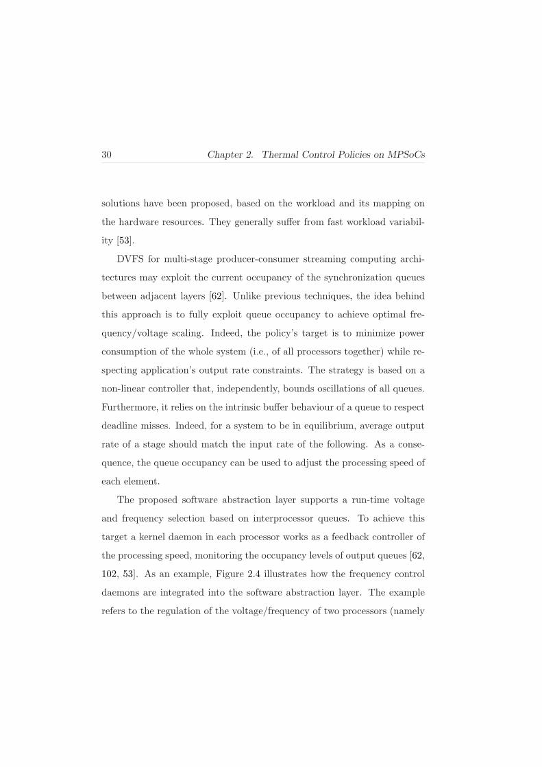
The proposed software abstraction layer supports a run-time voltage
and frequency selection based on interprocessor queues. To achieve this
target a kernel daemon in each processor works as a feedback controller of
the processing speed, monitoring the occupancy levels of output queues [62,
102, 53]. As an example, Figure 2.4 illustrates how the frequency control
daemons are integrated into the software abstraction layer. The example
refers to the regulation of the voltage/frequency of two processors (namely

2.3. Middleware Support in MPSoCs 31
N and N+1) running the tasks implementing two adjacent stages (stages N
and N+1) of a streaming pipelined application.
Figure 2.4: Distributed frequency regulation support implementation
Frequency controllers read the occupancy level of the communication
queues and select the proper voltage/frequency according to the selected
policy. The queues are integrated in the communication middleware as a
special message passing feature, because some dedicated functionalities are
needed to deal with the queues, as reading their occupancy level.

32 Chapter 2. Thermal Control Policies on MPSoCs
2.4 Control Feedback DVFS for Soft Real-Time
Streaming Applications
In this chapter I describe a control theoretic approach to dynamic voltage
ande frequency scaling (DVFS) in a pipelined MPSoC architecture with
soft real-time constraints, aimed at minimizing energy consumption with
throughput guarantees. The DVFS here described is part of the policy
developed for thermal control. Theoretical analysis and experiments are
carried out on a cycle-accurate, energy-aware, multiprocessor simulation
platform. A dynamic model of the system behavior is presented which al-
lows to synthesize linear and nonlinear feedback control schemes for the
run-time adjustment of the core frequencies. The characteristics of the
proposed techniques are studied in both transient and steady-state condi-
tions. Then, the proposed feedback approaches are compared with local
DVFS policies from an energy consumption viewpoint. Finally, the pro-
posed technique has been integrated on a multiprocessor operating system
in order to provide the Frequency/Voltage Management Support presented
in Section 2.3.
2.4.1 Introduction
Pipelined computing is a promising application mapping paradigm for low-
power embedded systems.
For instance, several multimedia streaming applications can be effi-

2.4. Control Feedback DVFS for Soft Real-Time Streaming Applications33
ciently mapped into pipelined Multi Processor System on Chip (MPSoC)
architectures [75]. Design and operation of pipelined MPSoCs subject to
soft real-time constraints entails conflicting requirements of high through-
put demand, limited deadline miss ratio and stringent power budgets.
Dynamic voltage/frequency scaling (DVFS) [77] is a well-known ap-
proach to minimize power consumption with soft real-time deadline guar-
antees. Here we address the problem of DVFS in pipelined MPSoCs with
soft real-time constraints by taking a feedback-based control-theoretic ap-
proach. We exploit the presence of buffers between pipeline stages to reduce
system power consumption. Buffers (also called FIFOs) are often used to
smooth the effects of instantaneous workload variations so as to ensure
stable production rates [96]. Intuitively, constant queue occupancy repre-
sents a desirable steady-state operation mode. Then, we use the occupancy
level of the queues as the monitored “output variables” [62, 102, 103] in
the feedback-oriented formalization of the problem. Constant queue occu-
pancy is difficult to achieve because of discretization of the available set of
voltages/frequencies, time granularity and unpredictable, possibly sudden,
workload variability.
The control objective to achieve is two-fold. First, the operating fre-
quency of each processor needs to be adjusted in such a way that the re-
quired data-throughput along the pipeline is guaranteed with minimum
oscillations of core clock frequency. Due to the square relationship between
power and frequency, this correspond to a desirable condition from a power

34 Chapter 2. Thermal Control Policies on MPSoCs
perspective. Small frequency oscillations can be achieved by enforcing small
fluctuations of the buffer occupancy levels. Furthermore, at the same time
it should be taken into account that rapid frequency switchings have a cost,
so their number should be kept as small as possible. Clearly, by reducing the
number of frequency switchings the queue fluctuations will become larger.
Then, the control problem involves conflicting requirements.
We first modeled the MPSoC as a set of interconnected dynamical sys-
tems. The model takes into account the discretization of frequency range.
Based on the given model, we designed linear (PI-based) and non-linear
feedback control techniques. The non-linear control strategy achieves a
theoretically-guaranteed robustness against the workload variations and
can decrease the rate of voltage/frequency adjustments drastically as com-
pared to the linear one.
We investigate, by means of theoretical analysis and experiments, the
inherent characteristics (energy saving, simplicity, robustness) of the pro-
posed feedback controllers, and give practical guidelines for setting their
tuning parameters. We also suggest proper ad-hoc modifications devoted
to alleviate some implementation problems.
In the experimental part of this work, the linear and non-linear feed-
back strategies are compared to local DVFS and shutdown policies by run-
ning benchmarks of pipelined streaming applications on a cycle-accurate,
energy-aware, multiprocessor simulation platform [64]. In the simulation
environment we have also taken into account a fixed frequency setting de-

2.4. Control Feedback DVFS for Soft Real-Time Streaming Applications35
lay. Experimental investigations show that feedback techniques outperform
the local DVFS policies in both transient and steady-state conditions.
It is worth noticing that our approach is application-independent and
can be extended to account for more complex architectures, e.g. two-
dimensional grids with a mesh interconnect, possibly involving interaction
of heterogeneous processing and communication elements.
Compared to [102, 103, 62], where queue dynamics are modeled only
using a single input queue, we formalized our model in case of multiple
processing stages. Moreover, instead of constraining the queue occupancy
level to be constant, we allow controlled fluctuations to minimize the en-
tity of frequency oscillations and switchings, leading to an efficient energy
behavior.
In our approach, we first consider a linear model of the queue dynamics
and we provide a thorough analysis of the feedback system with the simple
PI controller without any nonlinear mapping. Successively, we consider a
more general time-varying uncertain model and propose a novel nonlinear
feedback scheme. Proper ad-hoc methods (error thresholding and adaptive
sampling rate) are also developed to improve the controller performance.
This section is structured as follows. Section 2.4.2 introduces control
theoretic modeling, Section 2.4.3 deals with the linear controller analysis,
design and experiments, while Section 2.4.4 does the same for the non linear
controller. Description of the simulation environment is the matter of Sec-
tion 2.4.5, where some comparative experimental results are presented. On

36 Chapter 2. Thermal Control Policies on MPSoCs
Section 2.4.6 is presented the integration of the DVFS feedback controller
on the operating system.
2.4.2 Control-Theoretic DVFS Techniques for MPSoC
We consider MPSoC architectures in pipelined configuration. Each layer
contains a single processor, and two adjacent layers communicate by means
of stream data buffers according to the schematic representation in Fig-
ure 2.5 (the notation is explained throughout the Subsection 3.1).
P1 P2
Q1 Q2
f1
f2
kI1
kO2
f2kI2
PM
QM-1
fM-1
fMkOMf3
kI,M-1
kO3
Figure 2.5: M-layered pipelined architecture with inter-processor communication
queues
The core frequency fM of processor PM is considered as an assigned
parameter large enough depending on the current throughput specifications.
We deal with the design of feedback policies for the adjustment of the
core frequencies of processors P1, . . . PM−1. It seems reasonable to use the
occupancy level of the queues as the feedback signals driving the adaptation
policies [62, 103].

2.4. Control Feedback DVFS for Soft Real-Time Streaming Applications37
To decrease the input-output delay, the queue occupancy should be kept
as small as possible. This constitutes ad additional performance require-
ment.
System modeling
We now derive a dynamical model of the M-layered pipeline architecture
represented in Figure 2.5. Notation is defined as follows:
Qj : occupancy of the j-th buffer (1 ≤ j ≤ M − 1).
fi: clock frequency of the i-th processor (1 ≤ i ≤ M).
By definition, Qj is an integer non-negative number
Qj ∈ Q ≡ N ∪ {0} (2.1)
Due to technological aspects, in real systems the available speed values
fi can take on values over a discretized set FN . In particular, since fre-
quency adjustment is often made through pre-scalers [49], the set FN has
non-uniform spacing and usually contains a given “base frequency” fb and
a certain number of its sub-multiples, i.e.
fi ∈ FN ≡
{
fb,fbγ1
,fbγ2
, . . . ,fbγN
}
, γj ∈ N, γj < γj+1, j = 1, 2, . . . , N−1
(2.2)

38 Chapter 2. Thermal Control Policies on MPSoCs
Quantization of available frequencies (the adjustable “input variables”
of our system) represents a drawback from the control-theoretic point of
view.
To allow for a more straightforward use of classical control-theoretic
concepts we shall consider a continuous-time and real-valued model of the
queue occupancy. Let us define the following fictitious queue variable
Qj(t) Qj ∈ ℜ+ ∪ {0} (2.3)
and consider the following static memory-less piecewise-continuous nonlin-
ear map
Qj = projQ(Qj), (2.4)
where projY (X) is the projection operator mapping the input element X
on the closest element of the set Y . Roughly, mapping (2.4) “projects” the
auxiliary variable Qj onto the closest integer number.
As it can be seen from Figure 2.5, each processor gets its input data
from the “previous” queue and delivers output data by putting them into
the “next” queue. By using a queue-oriented notation, we shall refer to
the processor input and output data as “outcoming frames” and “incoming
frames”, respectively.
Denote as DOi (DIi) the outcoming (incoming) data-rate of the i-th
processor, i.e. the number of outcoming (incoming) frames processed in the
2.4. Control Feedback DVFS for Soft Real-Time Streaming Applications39
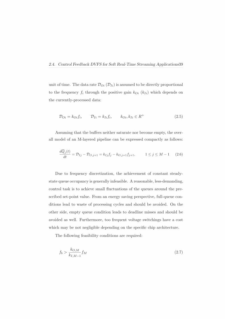
unit of time. The data rate DOi (DIi) is assumed to be directly proportional
to the frequency fi through the positive gain kOi (kIi) which depends on
the currently-processed data:
DOi = kOifi, DIi = kIifi, kOi, kIi ∈ R+ (2.5)
Assuming that the buffers neither saturate nor become empty, the over-
all model of an M-layered pipeline can be expressed compactly as follows:
dQj(t)
dt= DIj −DO,j+1 = kIjfj − kO,j+1fj+1, 1 ≤ j ≤ M − 1 (2.6)
Due to frequency discretization, the achievement of constant steady-
state queue occupancy is generally infeasible. A reasonable, less-demanding,
control task is to achieve small fluctuations of the queues around the pre-
scribed set-point value. From an energy saving perspective, full-queue con-
ditions lead to waste of processing cycles and should be avoided. On the
other side, empty queue condition leads to deadline misses and should be
avoided as well. Furthermore, too frequent voltage switchings have a cost
which may be not negligible depending on the specific chip architecture.
The following feasibility conditions are required:
fb >kO,M
kI,M−1fM (2.7)

40 Chapter 2. Thermal Control Policies on MPSoCs
kIj > kO,j+1, j = 1, 2, . . . ,M − 2 (2.8)
Conditions (2.7) and (2.8) guarantee that the incoming data rate of
each queue DIj can be made larger or smaller than the outcoming data rate
DO,j+1 by a proper setting of the frequency fj . Roughly, they guarantee
that each processor, when working at full speed, actually increases the
content of the successive queue.
The ideal steady-state condition is the perfect matching between the
incoming and outcoming data-rates of processors located at adjacent layers,
i.e.:
DIj = DO,j+1 =⇒ f∗j =
kO,j+1
kIjfj+1 (2.9)
Due to frequency discretization, it is generally impossible to run the pro-
ducer processor at the ideal frequency f∗ keeping constant the correspond-
ing queue occupancy. To formalize this concept, let f∗M be the frequency
of the consumer processor, and let f∗UP , f
∗LO be the adjacent frequencies
within the admissible set FN which satisfy the following condition
kI,M−1f∗LO < kO,Mf∗
M < kI,M−1f∗UP (2.10)
Running at the ideal frequency f∗ = (kO,M/kI,M−1)f∗M , lying between
f∗UP and f∗
LO, would make the producer data-rate to match the consumer

2.4. Control Feedback DVFS for Soft Real-Time Streaming Applications41
data-rate. The optimal steady-state time evolution of fM−1 is a periodic
square-wave between the values f∗UP , f
∗LO (see Figure 2.6)
t
*
UPf
*
LOf
*f
1−Mf
UPT LOT UPT LOT
Figure 2.6: The desired steady-state evolution of fM−1
Since the mean value of fM−1 should match the ideal frequency f∗,
the duty-cycle of the square wave depends on the distances f∗ − f∗LO and
f∗UP − f∗
LO according to the following formula:
TUP
TUP + TLO
=f∗ − f∗
LO
f∗UP − f∗
LO
(2.11)
To reduce the number of frequency switchings, the period of the square
wave should be as large as possible. Obviously, the larger the period of the
square wave, the larger the fluctuations of the queue.
Due to workload variations, the ideal frequency changes over time. Fluc-
tuations of the queue occupancy are acceptable as long as empty- or full-
queue conditions are avoided. For this reason, a desirable specification

42 Chapter 2. Thermal Control Policies on MPSoCs
for the feedback control system is its reactiveness, i.e. its capability to
quickly react to run time throughput/workload variations while avoiding
at the same time undesired phenomena such as, for instance, fast frequency
switching.
The main performance metrics we shall consider for evaluating and com-
paring the feedback controllers are the following:
• Reactiveness
• Number of voltage/frequency switchings.
• Ease of tuning
• Sensitivity to design parameters
• Computational complexity
Ease of tuning is a critical issue. Controllers are characterized by tun-
ing parameters that need to be set carefully to make the controller work
properly. For system designer, it is clearly desirable to play with a small
number of easy-to-tune parameters. Low sensitivity to design parameters
means essentially the controller capability of preserving satisfactory per-
formance by letting the controller parameters vary over a wide admissible
range.
Computational complexity must be considered mainly for two reasons.
First, the controller itself should have a negligible impact on the system

2.4. Control Feedback DVFS for Soft Real-Time Streaming Applications43
workload for stability reasons. Second, lower complexity helps in preserving
system predictability, which is a critical issue in embedded time-constrained
systems.
2.4.3 Linear analysis and design
If the workload is data-independent, and the buffers neither saturate nor
become empty, then coefficients kO,i and kI,i can be considered constant.
Thus, results from classical linear control theory can be profitably exploited
to design a feedback controller guaranteeing small fluctuations of the queue
occupancy.
The dynamics of the (M −1)-th queue is obtained by letting j = M −1
in the system (2.6):
dQM−1(t)
dt= kI,M−1fM−1 − kO,MfM (2.12)
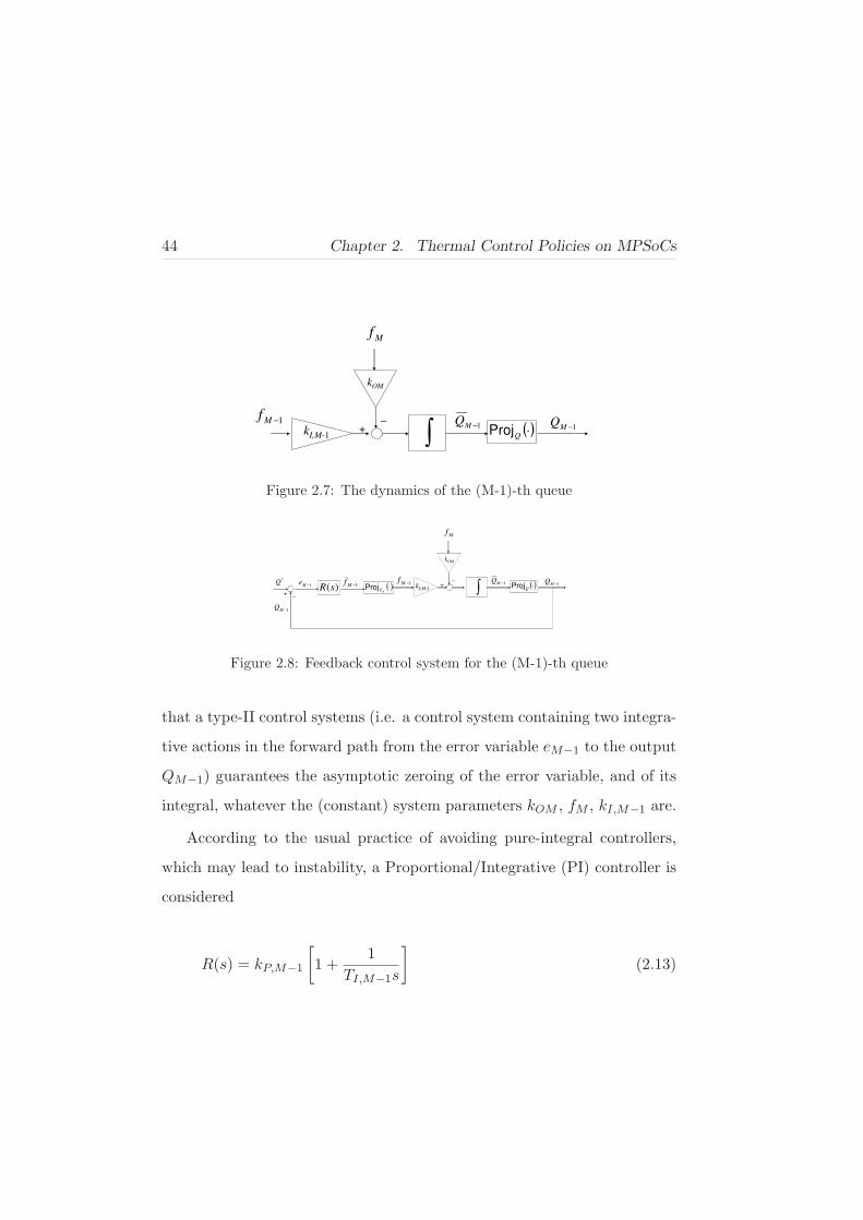
Such model can be represented by a standard block-diagram (see Fig-
ure 2.7).
LetQ∗ be the constant set-point for the queue occupancy. The “outcoming
data-rate” −kOMfM can be considered as a “disturbance” acting on the in-
put channel. The control system feedback architecture can be represented
as in Figure 2.8, where R(s) represents the transfer function of a generic
linear controller:
Neglecting the quantization operators, classical linear analysis tells us
44 Chapter 2. Thermal Control Policies on MPSoCs
∫ 1−MQkI,M-1
kOM
−+
Mf
1−Mf( )⋅QProj 1−MQ
Figure 2.7: The dynamics of the (M-1)-th queue
1−MQ−+
Mf
1−Mf
( )⋅QProj 1−MQ)(sR
*Q
+
1−MQ
−
1−Mf
( )⋅NFProj1−M
ekI,M-1
kOM
∫
Figure 2.8: Feedback control system for the (M-1)-th queue
that a type-II control systems (i.e. a control system containing two integra-
tive actions in the forward path from the error variable eM−1 to the output
QM−1) guarantees the asymptotic zeroing of the error variable, and of its
integral, whatever the (constant) system parameters kOM , fM , kI,M−1 are.
According to the usual practice of avoiding pure-integral controllers,
which may lead to instability, a Proportional/Integrative (PI) controller is
considered
R(s) = kP,M−1
[
1 +1
TI,M−1s
]
(2.13)

2.4. Control Feedback DVFS for Soft Real-Time Streaming Applications45
yielding the time-domain input-output relationship
fM−1(t) = kP,M−1
[
eM−1(t) +1
TI,M−1
∫
eM−1(τ)dτ
]
(2.14)
with the “tracking error” eM−1(t) being defined as eM−1(t) = Q∗−QM−1(t)
according to the notation used in the Figure 2.8. Constant parameters
kP,M−1 and TI,M−1 are referred to as the “proportional gain” and “integral
time” of the PI controller, respectively. The proportional gain principally
affects the “reactivity” of the controller, i.e. the duration of the transient,
while the integral time is mostly responsible for the transient characteristics,
such as, for instance, the amount of overshoot. As clarified in the experi-
ments, a large value of the proportional gain leads to unnecessary switching
activity in the steady state, thereby wasting energy and deteriorating the
overall performance. Then, setting of kp implies a conflict between transient
and steady-state specifications. An “optimal” controller tuning, maximiz-
ing some appropriate functional cost, should rely on the prior availability of
some information regarding the throughput, e.g. its statistical features. In
the control systems practice, however, trial-and-error tuning following sim-
ple qualitative guidelines gives often better performance, which motivates
our model-free approach.
Convergence analysis for the remaining queues is now addressed. We
have shown that the control system in Figure 2.8 with the PI controller
(2.13) guarantees the zeroing of eM−1, which implies a constant setting

46 Chapter 2. Thermal Control Policies on MPSoCs
of fM−1 in the steady state. Hence, the dynamics of the (M-2)-th queue
becomes formally equivalent to the representation in Figure 2.8, with fM−2
as the control input and fM−1 as the subtracting disturbance.
Then, the same convergence considerations apply, in sequence, to each
previous queues. Theoretically, a hierarchical “backward” convergence pro-
cess is guaranteed to occur, at the end of which each error variables ei has
been steered to zero.
In real systems, due to workload variations and frequency discretization,
the error variables ej cannot tend to zero, and the frequency of each proces-
sor, including that of the consumer processor fM , is generally time-varying.
This implies that the “disturbances” DO,j are also time-varying. Theo-
retically, the exact convergence is assured only when all disturbances are
constant. Nevertheless, due to the disturbance-rejection properties of the
integral-based control system in Figure 2.8, a bounded time-varying distur-
bance −kOMfM causes a bounded queue fluctuation, whose amplitude can
be affected through the controller gains. Such bounded fluctuation, further-
more, becomes negligible when the disturbance is slowly-varying compared
with the controller “reaction” time.
The algorithm for actual implementation of the PI control law (2.14),
to be run separately for each processor, is reported as follows. Integration
is discretized by the rectangular (zero-order hold) approximation. Let us
denote as ej [k] the error sample at the instant kTs, Ts being the sampling

2.4. Control Feedback DVFS for Soft Real-Time Streaming Applications47
interval, then
f j [k] = f∗j + kP,j
ej [k] +1
TI,j
Ts
h∑
ξ=0
ej [ξ]
(2.15)
The constant parameter f∗j allows to set a desired initial value of the
frequency. It should be set in such a way that f j [0] is as close as possible
to the ideal frequency f∗j (in general this is not possible due to lack of
informations regarding the consumer throughput). According to the scheme
in Figure 2.8, at every sampling time instant the “command” frequency
f j [k] is mapped on the closest element of the admissible set FN .
PI Controller Experimental Evaluation
We tested the performance of the PI-controlled system by implementing a
2-layered pipeline as that shown in Figure 2.9.
P1 Pc
Q1
f1
fc
kI1
kOc
kIc fc
Figure 2.9: 2-layered architecture

48 Chapter 2. Thermal Control Policies on MPSoCs
The frequency of the consumer processor is set to a constant value,
says fc, while the frequency of the producer is adjusted on-line through
feedback. The admissible set of frequencies used for experiments is:
f1 ∈ {200, 166, 142, 125, 111, 100, 90, 83, 77, 67, 59, 50, 42, 33, 20, 16, 8, 4}MHz
(2.16)
Producer P1 and consumer Pc execute a 2-stage pipelined application con-
sisting of a FIR filter and DES (Data Encryption System) encryption algo-
rithm.
P Controller To better investigate the inherent properties of linear feed-
back we first simulated a pure-proportional controller (TI = ∞). Sampling
time interval Ts has been set as small as possible (the control routine is
called each 100 µs). Simulation parameters are the queue size Qs, the pro-
portional gain Kp, and the consumer processor frequency fc. The set-point
is chosen as Q∗ = Qs/2.
The proportional gain has been set to a trial value with the queue size
taken large enough to avoid saturation effects. The parameters of the first
experiment are given as follows:
TEST1 : fc = 125MHz; kp = 20; Qs = 200 ⇒ Q∗ = 100 (2.17)
Results of TEST 1 are depicted in Figure 2.10. The abscissa is time

2.4. Control Feedback DVFS for Soft Real-Time Streaming Applications49
(µs) while the reported curves are the producer frequencies f1 (MHz) and
queue occupancy Q1.
Queue 1 occupancy (elements)
Processor 1 frequency (MHz)
Queue 1 occupancy (elements)
Processor 1 frequency (MHz)
Time [ µµµµs ]
Qu
eu
eEle
me
nts
/ M
Hz
Figure 2.10: The queue occupancy and producer frequency in the TEST 1
As expected, since there is no integral controller action, the mean value
of the error e1 = Q∗1 − Q1 does not vanish in steady state. This implies
that the queue occupancy Q1 oscillates around a value different from the
set-point Q∗.
Let us denote the mean value of e1 as e1MV . It can be computed by
considering the queue error equation, e1(t) = kI1f1−kOcfc, substituting for
the proportional adaptation law of f1, f1 = kpe1, and imposing condition
e1(t) = 0. It yields
e1MV =kOcfckI1kp
(2.18)
50 Chapter 2. Thermal Control Policies on MPSoCs
Then, kp needs to be large enough to keep the error mean-value well
below the queue saturation level Qs. This gives the closed loop system a
“robustness margin” useful for minimizing the probability of saturating or
empty queues.
When the consumer and producer processors execute the same opera-
tions there is matching between the gains kOc and kI1. Thus, they simplify
in eq. (2.18), which can be rewritten as follows
e1MV =fckp
(2.19)
The chosen experimental setup allows for the use the simplified formula
(2.19). By (2.17) and (2.19) the error mean value is:
e1MV = 6.25 (2.20)
which is in good agreement with the plot in Figure 2.10.
It is worth to highlight that in steady state the frequency does not
switch between two adjacent values. This is principally due to the integer
nature of Q1 and Q∗1, which implies that the error variable e1 can only
assume integer values. In steady state the error will eventually oscillate
around its mean value with amplitude, says, N :
ess = eMV + δ −N ≤ δ ≤ N (2.21)

2.4. Control Feedback DVFS for Soft Real-Time Streaming Applications51
The following condition should be met in order to prevent the controller
output f1 from “jumping” between non-adjacent values.
kp(eMV +N) < f∗UP kp(eMV −N) > f∗
LO (2.22)
In light of (2.18), it yields
kOcfckI1
+ kpN < f∗UP
kOcfckI1
− kpN > f∗LO (2.23)
Too small, or too large, values of kp cause unnecessarily large variations
of the producer frequency f1 in steady state. Keeping in mind that large
values of kp are useful to reduce the error, a sensible setting is as follows
kp ≈1
N
(
f∗UP −
kOcfckI1
)
(2.24)
Since in our tests there is matching between the gains kOc and kI1, eq.
(2.24) can be further manipulated as
kp ≈1
N(f∗
UP − fc) (2.25)
Let MINSP be the minimum spacing between adjacent frequencies of
the set (2.2). By (2.16), in the current experiments we have MINSP =
5MHz. A conservative tuning formula is as follows
kp ≈MINSP
N(2.26)

52 Chapter 2. Thermal Control Policies on MPSoCs
We investigated several settings of kp. In a second test (TEST 2) we
reduced the proportional gain kp leaving unchanged the other simulation
parameters:
TEST2 : fc = 125MHz; kp = 3; Qs = 200 ⇒ Q∗ = 100 (2.27)
Inspecting Figure 2.11 it can be observed that: (i) the mean value of
the error is eMV ≈ 40, which is according to the value predicted by (2.19);
(ii) the transient duration increases (i.e. reactiveness decreases); (iii) the
producer frequency oscillates between two adjacent values in the steady
state.
Time [ µµµµs ]
Qu
eu
eEle
me
nts
/ M
Hz
Queue 1 occupancy (elements)
Processor 1 frequency (MHz)
Queue 1 occupancy (elements)
Processor 1 frequency (MHz)
Figure 2.11: The queue occupancy and producer frequency in the TEST 2
Another test (TEST 3) was carried out to investigate the behavior of the
P controller when the queue maximal occupancy Qs is small. We reduced

2.4. Control Feedback DVFS for Soft Real-Time Streaming Applications53
it from 100 to 50 while keeping the same fc and kp values as those in TEST
2:
TEST3 : fc = 125MHz; kp = 3; Qs = 50 ⇒ Q∗ = 25 (2.28)
As shown in Figure 2.12, the producer frequency remains constant while
the queue remains empty. The reason is that the maximum error value
(eMAX = 25) is not high enough. As a result, the resulting producer
frequency f1 = kpeMAX = 75MHz cannot support the consumer data
rate. A larger value of kp would be needed to recover the stability, but
the amplitude of the voltage switching, and the probability of full-queue
condition, both increase.
Time [ µµµµs ]
Qu
eu
eEle
me
nts
/ M
Hz
Queue 1 occupancy (elements)
Processor 1 frequency (MHz)
Queue 1 occupancy (elements)
Processor 1 frequency (MHz)
Figure 2.12: The queue occupancy and producer frequency in the TEST 3
From the experimental analysis we obtained the following results re-
54 Chapter 2. Thermal Control Policies on MPSoCs
garding the pure-proportional controller:
• There is a finite, non-zero, error in steady state whose mean value is
affected by kp.
• kp needs to be sufficiently large to keep the error in steady- state
outside from the queue saturation and emptiness regions.
• kp needs to be sufficiently small, according to (2.23), to obtain steady-
state switches between adjacent frequency values. This requirement
impacts reactiveness.
PI controller Amajor improvement we expect by using the proportional-
integrative controller, with respect to the pure proportional one, is the ze-
roing of the error mean value eMV . The queue occupancy Q1 is therefore
expected to oscillate around the prescribed set-pointQ∗. Clearly, this would
enhance the control system robustness against rapid workload/throughput
variations by maximizing the distance from queue saturation/emptiness
conditions. This also helps in minimizing Q∗ to reduce the time delay
between the input and output data packets.
From theoretical analysis we can predict the unavoidable occurrence of
overshoot during the queue filling process. The reason is discussed as fol-
lows: in type-II control systems both the error and its integral are driven
asymptotically to zero. This implies the occurrence of overshoot because
the “positive” and “negative” areas (see Figure 2.13) need to compensate.

2.4. Control Feedback DVFS for Soft Real-Time Streaming Applications55
Using a time varying set point of the type Q∗(t) = Q∗(1− e−αt) the over-
shoot can disappear if the positive coefficient α is properly chosen.
t
+
-+
--
Q*
Q
Figure 2.13: Overshoot is necessary for compensating the negative and positive
areas
The qualitative guidelines given in the previous subsection for setting
the kp parameter are still valid. From condition eMV = 0, (2.24) is rewritten
as follows:
kp ≤1
Nf∗UP (2.29)
which is less stringent as compared to the previous case with eMV > 0. As
for the second controller parameter, the integral time (TI), it should princi-
pally affect the overshoot, the lower TI the larger the overshoot. Transient
duration also decreases by decreasing TI .
The additional parameter Ts, which represents the sampling step of
the discretized integration algorithm, now appears explicitly in the control
algorithm. Nevertheless, from (2.15) one can observe that for a given Ts
the ratio TI/Ts can be considered as an equivalent controller parameter.

56 Chapter 2. Thermal Control Policies on MPSoCs
We performed two experiments (TEST 4 and TEST 5) using two dif-
ferent values for TI , which is given relative to Ts.
TEST4 : fc = 125MHz; kp = 3; TI = Ts/6 Qs = 200 ⇒ Q∗ = 100
(2.30)
TEST5 : fc = 125MHz; kp = 3; TI = Ts/40 Qs = 200 ⇒ Q∗ = 100
(2.31)
Time [ µµµµs ]
Qu
eu
eEle
me
nts
/ M
Hz
Queue 1 occupancy (elements)
Processor 1 frequency (MHz)
Queue 1 occupancy (elements)
Processor 1 frequency (MHz)
Time [ µµµµs ]
Qu
eu
eEle
me
nts
/ M
Hz
Queue 1 occupancy (elements)
Processor 1 frequency (MHz)
Queue 1 occupancy (elements)
Processor 1 frequency (MHz)
Figure 2.14: The queue occupancy and producer frequency in the TEST 4 (left
plot, larger value of TI) and TEST 5 (right plot, smaller value of TI)
Comparing the two plots in Figure 2.14, the following considerations
arise:
2.4. Control Feedback DVFS for Soft Real-Time Streaming Applications57
• By reducing Ti, the overshoot increases while the transient speeds
up.
• The desired frequency square-wave reported in Figure 2.6 is ob-
tained in the steady state.
• Fast voltage/frequency switchings occur during the transient.
To investigate the sensitivity against the consumer frequency fc, we con-
sidered the same experimental conditions of the TEST 4 but we reduced fc
from 125MHz to 33MHz (TEST 6):
TEST6 : fc = 33MHz; kp = 3; TI = Ts/6 Qs = 200 ⇒ Q∗ = 100
(2.32)
The results of TEST 6 are shown in Figure 2.15. Higher overshoot, as
compared to the plot of TEST 4 (Figure 2.14-left), is obtained, and the
frequency switchings during steady state are more frequent.
The experimental investigation of the PI controller underlines the non-
trivial tuning of the TI parameter. The overshoot needs to be counteracted
in order to keep the system sufficiently far from the conditions of full or
empty queue. Deleterious fast switchings occur during transient and, less
frequently, also in the steady state. To reduce the number of frequency
switchings we can “relax” the control problem by allowing larger fluctua-

58 Chapter 2. Thermal Control Policies on MPSoCs
Time [ µµµµs ]
Qu
eu
eEle
me
nts
/ M
Hz
Queue 1 occupancy (elements)
Processor 1 frequency (MHz)
Queue 1 occupancy (elements)
Processor 1 frequency (MHz)
Figure 2.15: The queue occupancy and producer frequency in the TEST 6
tions of the queue. This can be achieved through a controller modification
(error thresholding) described in the next subsection.
PI controller with error thresholding The main drawbacks of the PI
controller are the possibly large overshoot and the fast frequency switchings
which are observed both during transient and in steady state.
To reduce the frequency switching activity we propose a thresholding
of the error variables. This modification lets the controller be active in
changing the producer frequency only when the error lies outside from a
dead-zone of thickness ∆. Thresholding is formalized as follows:
if |ej | ≤ ∆ then ej = 0, (2.33)
While the error is oscillating inside the dead-zone, which is a satisfactory

2.4. Control Feedback DVFS for Soft Real-Time Streaming Applications59
steady-state condition for the system, the producer frequency is “frozen”
since a PI controller with zero input keeps constant its output. The result-
ing fluctuations of the queue are not critical as long as Qs is sufficiently
large and the controller is sufficiently “reactive” outside the dead-zone.
We performed an experiment using the same parameters as those in
TEST 4 but introducing the error thresholding (2.33) with dead-zone thick-
ness of ∆ = 10:
TEST7 : fc = 125MHz; kp = 3; TI = Ts/6; Qs = 200 ⇒ Q∗ = 100, ∆ = 10
(2.34)
The results of TEST 7 are shown in Figure 2.16. They can be compared
to those of TEST 4 (Figure 2.14-left) since the controller parameters are the
same, except, obviously, the dead-zone thickness ∆. It can be observed a
consistent reduction of switching activity. As expected, the queue oscillates
approximately between the extreme values Q∗±∆ ≡ {90, 110}. It is worth
noting that we get the additional parameter ∆ to tune, which is not a
problematic issue due to its very intuitive meaning.
The PI controller behavior in a three layered architecture with 3 pro-
cessors (P1, P2 and the consumer PC) and 2 stream buffers (Q1, Q2) has

60 Chapter 2. Thermal Control Policies on MPSoCs
Time [ µµµµs ]
Qu
eu
eEle
me
nts
/ M
Hz
Queue 1 occupancy (elements)
Processor 1 frequency (MHz)
Queue 1 occupancy (elements)
Processor 1 frequency (MHz)
Figure 2.16: The queue occupancy and producer frequency in the TEST 7
been investigated. The queue dynamics are
dQ1
dt= kI1f1 − kO,2f2 (2.35)
dQ2
dt= kI2f2 − kOCfc (2.36)
Frequency f2 represents the control-input in the Q2 dynamics (2.36),
with the consumer frequency being treated as a disturbance input in the
stability analysis with follows the previously given guidelines. At the same
time, f2 represents the disturbance input in the Q1 dynamics (2.35), where
f1 plays the role of control input. This coupling between the queue dy-
namics can give rise to fast propagation of frequency oscillations, especially
when the consumer throughput changes rapidly and/or the throughput is
data-dependent. Error thresholding acts as a “low-pass” filter damping the
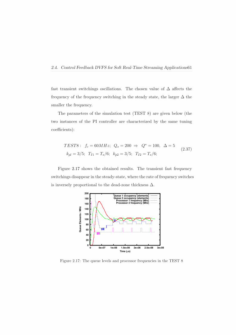
2.4. Control Feedback DVFS for Soft Real-Time Streaming Applications61
fast transient switchings oscillations. The chosen value of ∆ affects the
frequency of the frequency switching in the steady state, the larger ∆ the
smaller the frequency.
The parameters of the simulation test (TEST 8) are given below (the
two instances of the PI controller are characterized by the same tuning
coefficients):
TEST8 : fc = 60MHz; Qs = 200 ⇒ Q∗ = 100, ∆ = 5
kpl = 3/5; TI1 = Ts/6; kp2 = 3/5; TI2 = Ts/6;(2.37)
Figure 2.17 shows the obtained results. The transient fast frequency
switchings disappear in the steady-state, where the rate of frequency switches
is inversely proportional to the dead-zone thickness ∆.
0
20
40
60
80
100
120
140
160
180
200
0 5e+07 1e+08 1.5e+08 2e+08 2.5e+08 3e+08
Qu
eu
e E
lem
en
ts / M
Hz
Time (µs)
Queue 1 occupancy (elements)Queue 2 occupancy (elements)
Processor 1 frequency (Mhz)Processor 2 frequency (Mhz)
Figure 2.17: The queue levels and processor frequencies in the TEST 8

62 Chapter 2. Thermal Control Policies on MPSoCs
2.4.4 Non-linear analysis and design
Hereafter we explore a different class of controllers. We aim to partially
relax the linearity assumptions on the system model, to reduce the number
of tuning parameters and to achieve a more profitable trade-off between
reactiveness and voltage/frequency switching rate.
Consider again equation (2.6). If the workload is data-dependent then
parameters kOj and kIj are time-varying. It is reasonable to assume that
their actual value is limited between a known minimum and maximum:
0 < KOm,j ≤ kOj(t) ≤ KOM,j , 0 < KIm,j ≤ kIj(t) ≤ KIM,j (2.38)
The feasibility conditions (2.7)-(2.8) change as
fb >KOM,M
kIm,M−1fM kIm,j > kOm,j+1, j = 1, 2, . . . ,M − 2 (2.39)
Variation of the gains kOj and kIj can be used for modeling the oc-
currence of saturated or empty queues according to the following rules: if
the occupancy Qj saturates (Qj = Qs) then set kIj(t) = 0; if the buffer
Qj becomes empty (Qj = 0) then set kO,j+1(t) = 0. Sudden variations
of the gains can also capture the average effects of many other concurring
real-world phenomena. Thus, the dynamical model (2.6) with uncertain
time-varying gains can be considered a rather general model of the sys-
tem for the purpose of designing and analyzing a feedback-based DVFS

2.4. Control Feedback DVFS for Soft Real-Time Streaming Applications63
algorithm.
We augment model (2.6) by adding an integrator at the input side:
dQj(t)
dt= kIjfj − kO,j+1fj+1, 1 ≤ j ≤ M − 1
dfjdt
= wj
(2.40)
and we consider the derivative of fj , signal wj , as the new “control variable”
(see Figure 2.18).
S
1 1−MQkI,M-1
kOM
−+
Mf
1−Mf
( )⋅QProj 1−MQ
S
11−Mw
Figure 2.18: The “augmented” dynamics of the (M-1)-th queue.
Unlike the original control variable fj , which is nonnegative by defi-
nition, its derivative can assume both positive and negative value. The
dynamics of the error variable ej = Q∗ −Qj can be easily written as
dej(t)dt
= kIjfj − kO,j+1fj+1, 1 ≤ j ≤ M − 1
dfjdt
= wj
(2.41)
We propose the following feedback strategy for setting the control vari-

64 Chapter 2. Thermal Control Policies on MPSoCs
able wj :
wj = Gsign(ej) +Gsign(ej), sign(0) = 0, (2.42)
that can be rewritten as
wj =
2Gsign(ej) if ej ej > 0
0 if ej ej < 0
Gsign(ej) if ej = 0
Gsign(ej) if ej = 0
(2.43)
with G > 0 a controller parameter. The above control law can be seen
as a special realization of the “Twisting” algorithm [59] and belongs to
the class of control algorithms referred to as “second-order sliding-mode
controllers”, nonlinear control laws endowed by superior robustness prop-
erties against modeling errors, disturbances and non-idealities of various
kind [59, 9]. In actual implementation the sign of ej can be evaluated by
means of the sign of the difference between the current and past sample of
ej .
The rationale of controller (2.43) is best understood by analyzing the
physical meaning of the four conditions discriminated in (2.43) in which
different control actions are taken. Condition ej ej > 0 implies that the
modulus of the error is increasing. Thus frequency fj needs to be increased,
in the presence of a positive error, or decreased otherwise. This justifies

2.4. Control Feedback DVFS for Soft Real-Time Streaming Applications65
the first line of (2.43). Condition ej ej < 0 implies that the modulus of the
error is decreasing, which is a desirable transient condition that does not
require any frequency adjustment. This justifies the second line of (2.43).
If the error derivative is zero (i.e. the current and past queue occupancy
are coincident) the frequency is left unchanged if the error is zero, it is
increased in the presence of a positive error (Q1 < Q∗) and it is decreased
otherwise. In this way the controller performs an appropriate, and easily
justifiable, control action in each possible condition.
The actual behavior of the error and its derivative cannot be calculated
exactly since the system dynamics is uncertain. Nevertheless, it could be
formally proven that all solutions of the system (2.41)-(2.43) subject to the
inequalities (2.38)-(2.39) converge toward a small vicinity of zero. Some
intuitive stabilizing features, which constitute the basis of the convergence
analysis, are derived by the following simple qualitative analysis of the
closed loop behavior.
Typical system trajectories starting from the four “operating regions”
are reported in the Figure 2.19. Trajectories starting from any point even-
tually converge toward the axis ej = 0. Trajectories starting from the axis
ej = 0 can exhibit two different behaviors represented in Figure 2.19-B.
They can enter the region ej ej < 0 or come back to the region ej ej > 0.
This last situation occurs in the presence of sudden variations of the con-
sumer frequency. By exploiting the feasibility conditions (2.39) it is easy
to prove that only a finite number of rotations inside the “unstable region”

66 Chapter 2. Thermal Control Policies on MPSoCs
ej ej > 0 can occur, hence, after a finite time, the “stable region” ej ej < 0
is entered. By combining all together such behaviors it follows that the
error and its derivative enter an invariant rectangular domain containing
the origin.
0>jj ee �
0>jj
ee �
0>jjee �
0>jj ee �
0>jjee �
0>jjee �
0>jj ee �
0>jj ee �
0<jj ee �
0<jjee � 0<jj ee �
0<jj ee �
0<jj ee �
0<jjee �
0<jj ee �
0<jj ee �
Figure 2.19: Typical trajectories in the ej-ej plane
The special structure of the proposed controller allows for an effective
and easy implementation. Since in the actual context a positive or negative
“control input” wj can be understood as the requirements of increasing
(decreasing) the frequency, we can map positive/negative values of wj into
unit increment/decrement of the integer index i scaling the base frequency
fb such that it generates the current value of fj . Thus we do not need to
tune the parameter G. Care must be taken when selecting the sampling

2.4. Control Feedback DVFS for Soft Real-Time Streaming Applications67
period Ts, as discussed in the next subsection. It is apparent that the
computational complexity of this controller is much lower as compared to
the PI.
Nonlinear controller experimental evaluation
A 2-layered pipeline as that in Figure 2.9 was considered for the prelimi-
nary testing of the nonlinear controller. The unique controller tuning pa-
rameter is the sampling rate Ts at which the queue occupancy is read and
the corresponding control action is taken. Then, each experiment is fully
characterized by two parameters only, the producer frequency fc and the
controller sampling rate Ts
We made four experiments by combining two values for the consumer
frequency and sampling rate. Results are shown in Figure 2.20.
This analysis allows us to investigate parameter and throughput sensi-
tivity of the nonlinear controller. By increasing Ts we just obtain a slight
reduction of the voltage switchings in steady state and an overshoot in-
crease. The choice of Ts is critical since it is affected by the throughput
and at the same time it impacts heavily the rate of frequency switching. In
its current formulation, the nonlinear controller is thus rather sensitive to
the choice of the sampling rate.
As previously done to improve the PI performance, we consider the
error-thresholding to reduce the number of frequency switchings. This is

68 Chapter 2. Thermal Control Policies on MPSoCs
Time [ µµµµs ]
Qu
eu
eEle
me
nts
/ M
Hz
Queue 1 occupancy (elements)
Processor 1 frequency (MHz)
TEST 9: fc=166 MHz ; Ts=100 µµµµs
Time [ µµµµs ]
Qu
eu
eEle
me
nts
/ M
Hz
Queue 1 occupancy (elements)
Processor 1 frequency (MHz)
TEST 10: fc=166 MHz ; Ts= 400µµµµs
Time [ µµµµs ]
Qu
eu
eEle
me
nts
/ M
Hz
Queue 1 occupancy (elements)
Processor 1 frequency (MHz)
TEST 11: fc=33 MHz ; Ts=100 µµµµs
Time [ µµµµs ]
Qu
eu
eEle
me
nts
/ M
Hz
Queue 1 occupancy (elements)
Processor 1 frequency (MHz)
TEST 12: fc=33 MHz ; Ts=400 µµµµs
Figure 2.20: Nonlinear controller. Results of TESTS 9-12 with different consumer
frequency and sampling period.
the matter of next Subsection 5.2. In Subsection 5.3 we will also present an
ad-hoc controller modification, namely a mechanism for on-line adjustment
of Ts, which allows to replace the sampling rate with a different parameter
less sensitive to the operating conditions.

2.4. Control Feedback DVFS for Soft Real-Time Streaming Applications69
Nonlinear controller with error thresholding
A dead-zone mechanism like in (2.33) can smooth unnecessary switching
activity in the steady state. It results the simple scheme qualitatively de-
scribed in the Figure 2.21. The dead-zone “freezes” the frequency adapta-
tion when the error lies inside the range |ej | ≤ ∆. Note that increasing the
pre-scaler index one decreases the frequency and vice-versa, according to
the notation given in (2.2).
e
e&
KEEP THE SAME
FREQUENCY
KEEP THE SAME
FREQUENCYINCREASE THE
INDEX
DECREASE THE
INDEX
∆
-∆
Figure 2.21: Nonlinear control algorithm with error thresholding
Two experiments were made (TEST 13 and TEST 14) with the error-
thresholding having size ∆ = 20, the sampling period Ts = 100µs, and
two different consumer frequency values (fc1 = 166 MHz, fc2 = 33 MHz).
Except the ∆ value, the simulation parameters of TEST 13 and TEST 14
are the same as the TEST 9 and TEST 11, respectively (see Figure 2.20).
The results are depicted in the Figure 2.22. It is observed a considerable
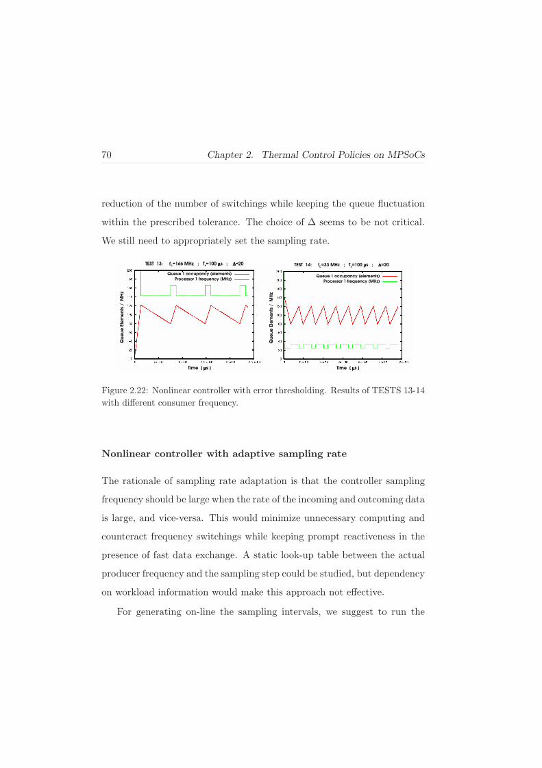
70 Chapter 2. Thermal Control Policies on MPSoCs
reduction of the number of switchings while keeping the queue fluctuation
within the prescribed tolerance. The choice of ∆ seems to be not critical.
We still need to appropriately set the sampling rate.
Time [ µµµµs ]
Qu
eu
eEle
me
nts
/ M
Hz
Queue 1 occupancy (elements)
Processor 1 frequency (MHz)
TEST 13: fc=166 MHz ; Ts=100 µµµµs ; ∆∆∆∆=20
Time [ µµµµs ]
Qu
eu
eEle
me
nts
/ M
Hz
Queue 1 occupancy (elements)
Processor 1 frequency (MHz)
TEST 14: fc=33 MHz ; Ts=100 µµµµs ; ∆∆∆∆=20
Figure 2.22: Nonlinear controller with error thresholding. Results of TESTS 13-14
with different consumer frequency.
Nonlinear controller with adaptive sampling rate
The rationale of sampling rate adaptation is that the controller sampling
frequency should be large when the rate of the incoming and outcoming data
is large, and vice-versa. This would minimize unnecessary computing and
counteract frequency switchings while keeping prompt reactiveness in the
presence of fast data exchange. A static look-up table between the actual
producer frequency and the sampling step could be studied, but dependency
on workload information would make this approach not effective.
For generating on-line the sampling intervals, we suggest to run the

2.4. Control Feedback DVFS for Soft Real-Time Streaming Applications71
control algorithm every time H new frames have been put in the queue.
Being the producer and consumer data rates closely related in the stable
steady state, the advantage of this approach is to achieve self-regulation
the sampling frequency according to the consumer throughput. The new
controller only depends on the parameter H, which is much easier to be set
as compared with the PI parameters and the constant sampling rate of the
non-linear controller.
The non-linear control law takes the form expressed in algorithm 1,
compactly referred as NL(e).
Algorithm 1 NL-ETA controllerEvery trigger instant do:
NL(e)
1: if e[k] < ∆ AND e[k] ≤ e[k − 1] then
2: increaseProducerFrequency()
3: else if e[k] > ∆ AND e[k] ≥ e[k − 1] then
4: decreaseProducerFrequency()
5: end if
We made four tests with the nonlinear controller using adaptive sam-
pling rate and error thresholding. We will choose this implementation of the
nonlinear controller for the final overall comparison. The strategy is com-
pactly referred to as Non-Linear Error-Thresholding Adaptive approach
(NL-ETA). The ∆ parameter was set to 20 and two values for the con-
sumer frequency and the H parameter were considered. Results are shown

72 Chapter 2. Thermal Control Policies on MPSoCs
in Figure 2.23. It is apparent from the comparison of the four plots that by
increasing H one obtains a reduction of the number if frequency switchings.
It can be also concluded that this property is preserved by changing the
consumer frequency. Then, the choice of H appears to be independent from
the throughput and workload, so the problem of finding a proper tuning
for the H parameter in the NL-ETA scheme is much easier as compared
with the problem of tuning the sampling period Ts in the original nonlinear
scheme with a constant step.
Time [ µµµµs ]
Qu
eu
eEle
me
nts
/ M
Hz
Queue 1 occupancy (elements)
Processor 1 frequency (MHz)
TEST 15: fc=166 MHz ; H=10 ; ∆∆∆∆=20
Time [ µµµµs ]
Qu
eu
eEle
me
nts
/ M
Hz
Queue 1 occupancy (elements)
Processor 1 frequency (MHz)
TEST 16: fc=166 MHz ; H=3 ; ∆∆∆∆=20
Time [ µµµµs ]
Qu
eu
eEle
me
nts
/ M
Hz
Queue 1 occupancy (elements)
Processor 1 frequency (MHz)
TEST 17: fc=33 MHz ; H=10 ; ∆∆∆∆=20
Time [ µµµµs ]
Qu
eu
eEle
me
nts
/ M
Hz
Queue 1 occupancy (elements)
Processor 1 frequency (MHz)
TEST 18: fc=33 MHz ; H=3 ; ∆∆∆∆=20
Figure 2.23: NL-ETA controller. Results of TESTS 15-18 with different consumer
frequency and H parameter.

2.4. Control Feedback DVFS for Soft Real-Time Streaming Applications73
Another test (TEST 19) considered a three-layered architecture with
3 processors and 2 data stream buffers. The consumer frequency was set
to 60MHz. The NL-ETA parameters are ∆ = 20, H = 10. Figure 2.24
reports the attained, satisfactory, results.
0
20
40
60
80
100
120
140
160
180
200
0 5e+07 1e+08 1.5e+08 2e+08 2.5e+08 3e+08
Qu
eu
e E
lem
en
ts / M
Hz
Time (µs)
TEST 19: fc = 60 MHz; H = 10; ∆ = 20
Queue 1 occupancy (elements)Queue 2 occupancy (elements)
Processor 1 frequency (Mhz)Processor 2 frequency (Mhz)
Figure 2.24: NL-ETA controller in a three-layer architecture. Results of TEST 19.
2.4.5 Experimental Validation on a Cycle-Accurate Plat-
form
Simulation Environment
The benchmark applications used for the experimental comparison run on
a cycle-level accurate, energy-aware, multi-processor simulation platform.
We carried out our analysis within the framework of the SystemC-based
MPARM platform [64]. Figure 2.25 gives a schematics of the simulated

74 Chapter 2. Thermal Control Policies on MPSoCs
Figure 2.25: MPSoC platform with hardware support for frequency scaling.
architecture. It consists of a configurable number of 32-bit ARMv7 proces-
sors. Each processor core has its own private memory, and a shared mem-
ory is used for inter-processor communication. Synchronization among the
cores is provided by hardware semaphores implementing the test-and-set
operation. The system interconnect is a shared bus instance of the STBus
interconnect from STMicroelectronics. It can be directly manage hardware
semaphores for synchronization between processors.
The virtual platform environment provides power statistics made avail-
able by STMicroelectronics for a 0.13 µm technology in ARM cores, caches,
memories and STBus.
Benchmark applications
Each application is a sequence of standard algorithms for signal processing
(FIR filtering) and cryptography (DES encryption-decryption) applied to

2.4. Control Feedback DVFS for Soft Real-Time Streaming Applications75
a vector of samples. 2-stage and 3-stage pipelines have been considered.
To obtain variable workload applications dummy loops are added into
the FIR and DES routines to reproduce artificial data dependency. The
workload variability due to the dummy loops introduction, expressed via
the worst-case execution cycles vs. average case, has been estimated as
near 60%.
A frequency setting delay of 10 µ s is included in the simulation model
but no energy cost is associated to the frequency adjustments. The CPU
load of all considered control routines appears to be negligible as compared
with the main applications.
Comparative Results
The feedback control techniques described in previous sections have been
extensively characterized and compared. A first set of experiments has been
performed to compare the linear PI and non-linear NL-ETA controllers. A
second set of experiments was targeted to the energy efficiency.
Linear vs. nonlinear controller implementation In previous sec-
tions some limitations of the PI controllers in terms of difficult parameter
settings and excessive switching rate have been discussed. The latter phe-
nomenon may have an important cost in terms of energy consumption.
In steady-state, PI controllers suffer from the intrinsic performance limi-
tations listed at the end of Subsection 4.1.1. A low kp impacts the controller

76 Chapter 2. Thermal Control Policies on MPSoCs
reactiveness, so that the condition of full or empty queue is more likely to
occur. A large kp causes instead large frequency oscillations. In Figure 2.26-
left kp is too small (kp = 0.6) and the queue becomes full due to limited
reactiveness. In Figure 2.26-right, kp has been increased (kp = 3) thereby
avoiding the saturation but causing larger oscillations of the producer fre-
quency. An optimal choice for kp is thus not easy to find.
In Figure 2.27 we show the results obtained using the NL-ETA. The
fast frequency switchings observed during the PI transient in Figure2.26-
right totally disappeared, which seems to confirm that the nonlinear con-
trol method offers the best compromise between reactiveness and rate, and
amount, of input frequency oscillations.
Time [ µµµµs ]
Qu
eu
eEle
me
nts
/ M
Hz
Queue 1 occupancy (elements)
Processor 1 frequency (MHz)
TEST 20: fc=33 MHz ; ∆∆∆∆=5 ; kp=0.6 ; TI=Ts/6
Time [ µµµµs ]
Qu
eu
eEle
me
nts
/ M
Hz
Queue 1 occupancy (elements)
Processor 1 frequency (MHz)
TEST 21: fc=33 MHz ; ∆∆∆∆=5 ; kp=3 ; TI=Ts/6
Figure 2.26: PI controller with error thresholding (fc = 33 MHz and ∆ = 5). Left
plot: kp = 0.6. Low reactiveness with small steady-state oscillations. Right plot:
kp = 3. High reactiveness with large steady-state oscillations.

2.4. Control Feedback DVFS for Soft Real-Time Streaming Applications77
Time [ µµµµs ]
Qu
eu
eEle
me
nts
/ M
Hz
Queue 1 occupancy (elements)
Processor 1 frequency (MHz)
TEST 22: fc=33 MHz ; ∆∆∆∆=20 ; H=3
Figure 2.27: NL-ETA controller ( fc = 33 MHz,∆ = 20, H = 3): high reactiveness
with small steady-state oscillations.
Energy saving tests Experiments were performed using the energy con-
sumption and the rate of frequency adjustments as the main metrics for
comparison. The single-core configuration, as well as local DVFS policies
(ON-OFF and Vertigo) were included in the comparative analysis. We
have made four tests: we considered a 2-layer and a 3-layer pipeline under
both stable and variable workload. As previously stated, variable workload
is reproduced by the random execution of dummy instruction loops. For
each test, many techniques are implemented and their performances are
compared.
A baseline setup in which all tasks are mapped into a single core was
first considered for the purpose of comparison. We also implemented an or-

78 Chapter 2. Thermal Control Policies on MPSoCs
acle policy (ON-OFF) shutting-down the appropriate processor(s) in pres-
ence of empty- or full-queue conditions. As local DVFS, we considered
the frequency setting algorithm used in standard ARM Intelligent Energy
Manager enabled systems (IEM), called “VERTIGO” policy [48] [34].
We implemented the feedback-based PI with error thresholding (PI-ET)
and the nonlinear controller with error thresholding and adaptive sampling
(NL-ETA). The values of the chosen metrics are shown in Table 2.1. We
evaluated the energy required to process a pre-specified amount of data
with assigned throughput. We computed separately the total system energy
(cores, memories, caches, busses) and the energy separately required by the
processors whose frequency is run-time adjusted.
Results of Table 2.1 highlight that the linear and nonlinear feedback
controllers outperform the static methods, while they are comparable with
each other, from the energy consumption viewpoint. However, it shall be
noted that no energy cost is associated to the frequency switching. Thus,
the nonlinear controller, which reduces significantly the number (N sw.) of
voltage switchings, can be considered as the most effective one.
2.4.6 Operating System Integration of the DVFS Feedback
Controller
Dynamic voltage scaling algorithms have been widely implemented in sin-
gle processor systems. In some cases they are embedded in the OS. ARM

2.4. Control Feedback DVFS for Soft Real-Time Streaming Applications79
2-stages - stable workload
core1 core2 total N
Technique energy energy energy sw.
(mJ) (mJ) (mJ)
Single Core 1044 - 2422 -
ON-OFF 488 - 2148 -
Vertigo 1054 - 2876 -
PI-ET 216 - 1917 10
NL-ETA 214 - 1910 7
2-stages - variable workload
core1 core2 total N
Technique energy energy energy sw.
(mJ) (mJ) (mJ)
ON-OFF 750 - 2874 -
Vertigo 1194 - 3357 -
PI-ET 530 - 2665 16
NL-ETA 525 - 2660 15
3-stages - stable workload
core1 core2 total N
Technique energy energy energy sw.
(mJ) (mJ) (mJ)
Single Core 1396 - 3232 -
ON-OFF 428 430 2799 -
Vertigo 563 554 3143 -
PI-ET 245 195 2410 42
NL-ETA 242 192 2400 21
3-stages - variable workload
core1 core2 total N
Technique energy energy energy sw.
(mJ) (mJ) (mJ)
ON-OFF 574 430 2984 -
Vertigo 742 554 3248 -
PI-ET 359 200 2644 70
NL-ETA 351 202 2637 44
Table 2.1: Control techniques comparison

80 Chapter 2. Thermal Control Policies on MPSoCs
Intelligent Energy Manager (IEM) is an example of an integrated voltage
scaling solution [48]. However, when targeting multicore platforms run-
ning data-flow oriented applications, traditional approaches that looks at
the local processor utilization are not longer efficient because of two main
reasons. First, they disregard the interaction between processing elements
and between data producer and consumers, being the utilization an indirect
function of the throughput required by the whole application. Second, the
reaction to workload variations are not efficient, since they do not take into
account the presence of communication buffers that may smooth processing
peaks.
In this section we describe the extension of the control algorithm to han-
dle configurations with multiple tasks on each processor. As case study, we
focus on a software FM Radio application composed by six communicating
tasks. The application is described more in details in Section 2.4.6. From
a power viewpoint, the optimal mapping of these tasks into processing ele-
ments depends on the required frame rate and on the number of available
processors.
The application is organized into 4 stages, following the configuration
described in Figure 2.28, with a variable output frame rate, depending on
the wanted sound quality. We considered to have a maximum of 3 available
processors, a set of five available frequencies for each processor and an
external audio peripheral acting as a consumer that imposes the output
data-rate.

2.4. Control Feedback DVFS for Soft Real-Time Streaming Applications81
Figure 2.28: FM Radio
a) b) c)
Figure 2.29: Optimal application mapping scenarios
As we will see in the experimental result section, three optimal task-
processor mappings can be identified that covers the whole range of sus-
tainable frame rates. They are described in Figure 2.29.
The configurations are optimal from the point of view of energy effi-
ciency, depending on the required frame rate, as explained in Section 2.4.6.
Being equal to eight the total number of queues to monitor, considering
the most complex case where three processors are running, the number of
adjustable control variables (i.e. the frequencies) is three. When the num-
ber of monitored variables is larger than the number of available control

82 Chapter 2. Thermal Control Policies on MPSoCs
actions, it is said that the system is “underactuated”, and the associated
control problems are more challenging.
To explain the proposed solution, let us take the configuration c) of
Figure 2.29 as an example. We can write the dynamics of the queues as
follows:
Q1(t) = kIp0(t)fp0 − kOp1(t)fp1
Q21(t) = kIp1(t)fp1 − kOp0(t)fp0
Q22(t) = kIp1(t)fp1 − kOp2(t)fp2
Q23(t) = kIp1(t)fp1 − kOp2(t)fp2
Q31(t) = kIp0(t)fp0 − kOp0(t)fp0
Q32(t) = kIp2(t)fp2 − kOp0(t)fp0
Q33(t) = kIp3(t)fp2 − kOp0(t)fp0
Q4(t) = kIp3(t)fp0 − FR
(2.44)
The overall aim is to develop a control law able to prevent emptiness
condition for any of the queues, thus avoiding the risk of QoS degradation
due to frame misses. On the other side, a trivial solution where all of the
queues are full is not optimal from an energy perspective. The optimal
frequency must be selected depending on the values of the outgoing queues
of each processing element. There is no obvious choice for selecting an
appropriate error variable, as it generally happens in the underactuated
control problems.
We propose to use the following generalized form of the time variant

2.4. Control Feedback DVFS for Soft Real-Time Streaming Applications83
NL control algorithm, which defines the frequency of the i− th processor.
fpi = NL(AUXi −Q∗) (2.45)
The auxiliary variable AUXi − Q∗ is defined in order to consider the
minimum between the occupancy levels of the queues fed by the tasks
running in the processor i:ed by the tasks running in the processor i:
AUXi = min {Qa, Qb, .., Qn} (2.46)
where Qa, Qb, .., Qn are the queues fed by tasks running in the processor
i.ed by tasks running in the processor i.
Using logic (2.45), (2.46) the frequency of each processor is run time set
to keep under control the queue which is closest to the emptiness condition.
During stable operation, the minimum value will be close to the current
occupancy of all queues. It is evident that this kind of control law can be
always applied independently from tasks-processor mapping configuration
and from the underlying OS scheduler.
Middleware-level Implementation
In this section we first describe the target architecture, then we explain the
integration of the algorithm.
84 Chapter 2. Thermal Control Policies on MPSoCs
Target Architecture and OS/Middleware The target architecture,
the application class used as reference and the middleware support are all
described in Sections 2.2 and 2.3.
DVFS Feedback Control Algorithm Integration The controller was
embedded in the write system call made available as a interprocessor com-
munication interface. A write system call is performed whenever a task
wants to pass a data item to another processor. Before each write opera-
tion, that is, each time a new element is pushed into an outgoing queue,
the following operations are performed:
AUXi PTR is the pointer to the emptiest queue. This pointer is ini-
tialized at the beginning by scanning all the queues and than is updated
every time an element is added to a queue according to the previous algo-
rithm. The condition |∆Q| > H represents the triggering condition, that
is true when a variation greater than H occurs on the occupancy level of
the queue. This way, the control algorithm is triggered only when needed
as a consequence of a write operation on the relative queue.
Experimental results
Emulation Platform Description For the simulation and performance
evaluation of the proposed middleware, we used an FPGA based, cycle accu-
rate, MPSoC hardware emulator [16] built on top of the Xilinx XUP FPGA
board [50], and described in Figure 2.30. Time and energy data are run-

2.4. Control Feedback DVFS for Soft Real-Time Streaming Applications85
Algorithm 2 Control Feedback Algorithm Integration1: if the current queue level is LOWER than the queue level referenced by the
AUXi PTR then
2: The AUXi PTR is updated to point at the current queue
3: end if
4: if the current queue is the same queue pointed by the AUXi PTR then
5: NL control algorithm:
6: if |∆Q| > H then
7: if [ ei > Z AND ei ≥ ei,PREV ] then
8: decreaseFrequency()
9: else if [ ei < −Z AND ei ≤ ei,PREV ] then
10: increaseFrequency()
11: end if
12: end if
13: end if

86 Chapter 2. Thermal Control Policies on MPSoCs
Figure 2.30: Overview HW architecture of emulated MPSoC platform
time stored using a non-intrusive, statistics subsystem, based on hardware
sniffers which stores frequencies, bus and memory accesses. A PowerPC
processor manages data and control communication with the host PC us-
ing a dedicated UART-based serial protocol. Run-time frequency scaling is
also supported and power models running on the host PC allow to emulate
voltage scaling mechanism. Frequency scaling is based on memory-mapped
frequency dividers, which can be programmed both by microblazes or by
PowerPC. The power associated to each processor is 1 Watt for the max-
imum frequency, and scales down almost cubically to 84 mW as voltage
and frequency decrease. Power data refer to a commercial embedded RISC
processor and are provided by an industrial partner. The emulation plat-
form runs at 1/10 of the emulated frequency, enabling the experimentation
of complex applications which may be not experimented using software
simulators with comparable accuracy.

2.4. Control Feedback DVFS for Soft Real-Time Streaming Applications87
Test Application Description To evaluate the effectiveness of the pro-
posed support on a real test-bed we ported to our system a software FM
radio benchmark, that is representative of a large class of streaming mul-
timedia applications following the split-join model [92] with soft real-time
requirements. It allows to evaluate the trade-off between the long-term
performance improvement given by migration-enabled run-time task remap-
ping and the short-term overhead and performance degradation associated
to migration.
As shown in Figure 2.28, the application is composed by various tasks,
graphically represented as blocks. Input data represent samples of the dig-
italized PCM radio signal which has to be processed in order to produce
an equalized base-band audio signal. In the first step, the radio signal
passes through a Low-Pass-Filter (LPF) to cut frequencies over the radio
bandwidth. Then, it is demodulated by the demodulator (DEMOD) to
shift the signal at the baseband and produce the audio signal. The audio
signal is then equalized with a number of Band-Pass-Filters (BPF) im-
plemented with a parallel split-join structure. Finally the consumer (Σ)
collects the data provided by each BPF and makes the sum with different
weights (gains) in order to produce the final output.
Since each BPF of the equalizer stage acts on the same data flow, the
demodulator has to replicate its output data flow writing the same packet
on every output queue.
Thanks to our platform, we could measure the workload profile of the

88 Chapter 2. Thermal Control Policies on MPSoCs
various tasks. We verified that the most computational intensive stage is
the demodulator, imposing a CPU utilization of 45% of the total, while for
the other tasks we observed respectively 5% for the LPF, 13% for each BPF
and 5% for the consumer. This information will be used by the implemented
migration support to decide which task has to be migrated.
Energy efficient configurations are computed starting from energy vs
frame rate curves. Each curve represents all the configurations that are
obtained by keeping the same number of processors while increasing the
frequency to match the desired frame rate. Then we take the Pareto con-
figurations that minimize energy consumption for a given frame rate. The
minimum allowed processor frequency in our case is 100 MHz. The power
consumed by the cores as a function of the frame rate is shown in Fig-
ure 2.31. The plot shows three curves obtained by computing the power
consumed when mapping the FM Radio tasks in one, two or three cores.
In order to determine the best power configuration for each frame rate
we computed the Pareto points, as shown in Figure 2.32. Intuitively, when
the frame rate increases, a higher number of cores is needed to get the
desired QoS in a energy efficient way.
DVFS Controller Behavior Description To illustrate the behavior
of the controller, Figures 2.33.a and b show the evolution of processor fre-
quency and queue occupancy level of the emptiest and last queue of the
application (configuration (a) in Figure 2.29). The emptiest queue in this
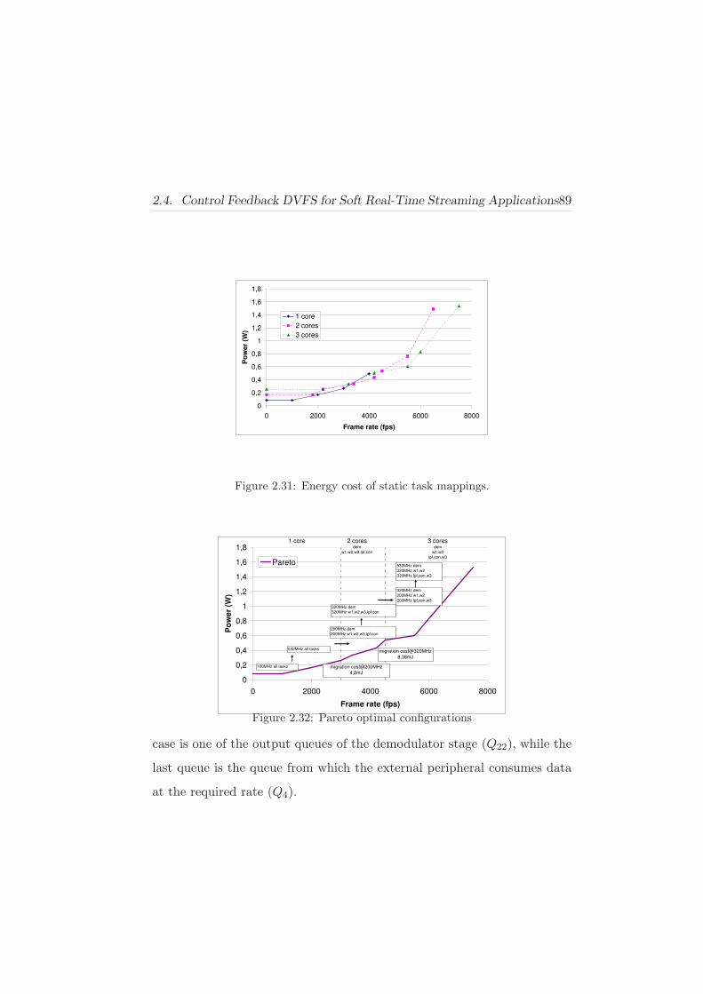
2.4. Control Feedback DVFS for Soft Real-Time Streaming Applications89
0
0,2
0,4
0,6
0,8
1
1,2
1,4
1,6
1,8
0 2000 4000 6000 8000
Frame rate (fps)
Po
we
r (W
)
1 core
2 cores
3 cores
Figure 2.31: Energy cost of static task mappings.
0
0,2
0,4
0,6
0,8
1
1,2
1,4
1,6
1,8
0 2000 4000 6000 8000
Frame rate (fps)
Po
we
r (W
)
Pareto
1 core 2 coresdem
w1,w2,w3,lpf,con
3 coresdem
w1,w2
lpf,con,w3
532MHz all tasks
320MHz dem
320MHz w1,w2,w3,lpf,con
100MHz all tasks
200MHz dem
200MHz w1,w2,w3,lpf,con
320MHz dem
200MHz w1,w2
200MHz lpf,con,w3
532MHz dem
320MHz w1,w2
320MHz lpf,con,w3
migration cost@200MHz
4,2mJ
migration cost@320MHz
8,38mJ
Figure 2.32: Pareto optimal configurations
case is one of the output queues of the demodulator stage (Q22), while the
last queue is the queue from which the external peripheral consumes data
at the required rate (Q4).

90 Chapter 2. Thermal Control Policies on MPSoCs
(a) (b)
Figure 2.33: Queues occupancy and processor frequency for single processor con-
figuration: a) H = 5;Z = 5 ; b) H = 4;Z = 10. Actual frequencies (shown) are
1/10 of emulated frequencies.
Two different configurations are considered for the parameters of the
controller: H = 5 and Z = 5, in plot a, while H = 4 in Z = 10 for plot b.
It is worth noting how the level of the emptiest queue is kept under control,
showing an occupancy level always close to the ”dead zone”. On the other
side, the last queue Q4 is always full, because the preceding stages of the
application are providing enough data. The proposed mechanism lets the
processor frequency to switch between the two available frequencies around
the ideal frequency needed to provide the required data rate required by the
application. This is a highly desirable condition. Comparing plots a and b
in Figure 2.33, it can be noted that increasing Z (that is, the size of the
dead zone) lead to a reduction of the oscillations of the queue occupancy
level, thus reducing frequency switchings.
2.4. Control Feedback DVFS for Soft Real-Time Streaming Applications91
DVFS Controller Efficiency Evaluation In this section we show the
comparison of the efficiency of the proposed distributed control strategy
against a local policy based on the well known Vertigo performance set-
ting algorithm [34] used in the ARM-IEM standard [48]. Each processor
runs locally the Vertigo algorithm. The comparison is made in terms of
energy efficiency and in terms of numbers of switchings. In Figure 2.34
two plots are shown comparing the normalized mean energy consumed by
the system. The plots show how the energy consumed by NL controller is
half of the energy consumed using the local policy, independently from the
values chosen for the parameters of the NL controller. This improvement
can be justified by the following observation. Let us define the slack as
the amount of idleness that a processor experiences when running at the
maximum frequency. The feedback control technique is able to efficiently
assign the slack to the most urgent task, that is the one with the emptiest
queue. On the other side, a local policy does not have knowledge of the
queue occupancy level, leading to a suboptimal slack assignment.
Moreover, the proposed controller is robust with respect to parameter
tuning. To highlight this property, a sweep on Z and H values is shown
in Figure 2.34. The values are averaged over the results obtained using
the three system configurations depicted in Figure 2.29, and considering
several values of frame rate required by the application. The energy values
are normalized considering with respect to the average energy consumed
using the ARM-IEM policy.

92 Chapter 2. Thermal Control Policies on MPSoCs
(a) (b)
Figure 2.34: Energy efficiency comparison between local and NL controllers: (a)
sweep on H; (b) sweep on Z
In Figure 2.35 two plots are shown comparing the average number of
frequency switchings per second of each processor. The plots show how
the number of switchings due to the NL controller is always less than the
one due to the local policy, independently from the values chosen for the
parameters of the NL controller. It is worth to note from plot (b) that with
the increase of the dead zone (Z increases) the switching activity decreases.
2.5 Thermal Balancing for Stream Computing: MiGra
In general, thermal balancing does not come as a side effect of energy bal-
ancing. In Figure 2.36.a, a typical situation where a two-core system run-
ning three tasks (A, B, C) is energy-balanced (but thermally-unbalanced)
is shown. Both processors can independently set their frequency and volt-
age to reduce energy/power dissipation to the minimum required by the

2.5. Thermal Balancing for Stream Computing: MiGra 93
(a) (b)
Figure 2.35: Frequency switchings comparison between local and Nl controllers:
(a) sweep on H; (b) sweep on Z
current load. Tasks are characterized by their Full-Speed-Equivalent (FSE)
load, which is the load imposed by a task when the core runs at maximum
frequency. Core 1 runs tasks A and B, having FSE of 50% and 40% re-
spectively; core 2 runs task C that has a FSE of 40%. In this case core 1
can ideally scale its frequency to 90% of its maximum value, while core 2
can scale it to 40%. No better tasks mapping exists that further reduces
energy/power dissipation. In this situation, due to the different power con-
sumed, the temperature of core 1 will be higher than the temperature of
core 2. Therefore, a thermally balanced condition can be achieved by pe-
riodically migrating task B from the first core to the second core [104] (as
represented in Figure 2.36.b), obtaining, on average, an equalized workload
on the two cores (i.e., 40% +50%/2 = 65%). If the temperature variations
caused by migrations are slower than the migration period, a temperature
close to the average workload (i.e, 65%) will be achieved on both cores.

94 Chapter 2. Thermal Control Policies on MPSoCs
Although this is a simplified case, it outlines that the main challenge of
a thermal balancing algorithm is the selection of the task sets to migrate
between two or more cores, such that that overall temperature is balanced,
while keeping migration costs bounded.
Figure 2.36: Simple thermal balancing example
2.5.1 MiGra: Thermal Balancing Algorithm
The thermal balancing strategy we propose in this work, MiGra, is inspired
by [17]. To prevent impact on QoS caused by migrations, MiGra is based on
run-time estimation of migration costs to filter migration requests driven by
temperature differences between cores. Thus, MiGra considers performance
and energy migration costs caused by the underlying migration infrastruc-
ture (cf. Section 2.3). Moreover, in our implementation, MiGra lies on top

2.5. Thermal Balancing for Stream Computing: MiGra 95
of a Dynamic Voltage and Frequency scaling (DVFS) policy [27]. Thus,
the power consumption of a task can be roughly estimated at run-time by
assuming that it is proportional to its load (cf. Figure 2.2).
MiGra implements a strategy that tries to bound the temperature of
each processor around the current average temperature, as well as mini-
mizing the overhead in terms of number of migrated tasks and amount of
data transferred between the cores due to migrations. Therefore, a maxi-
mum distance of the temperature of each processor from the current average
temperature is defined by MiGra, identifying a range of permissible temper-
atures for each single processor between an upper and a lower threshold.
These thresholds are dynamically adapted at run-time according to the cur-
rent workload. MiGra also control thermal runaway by stopping the core
that reaches a temperature above a predefined panic threshold. Nonethe-
less, this extreme situation should never occur in realistic streaming ap-
plications, and MiGra’s regular operation always keeps its upper threshold
below this panic one, by trying to minimize temperature gradients. Each
time the temperature of a processor reaches the upper threshold around the
average temperature of the MPSoC platform, MiGra triggers a migration
to move away a set of tasks from the hot processor to another processor
having a temperature below the current average temperature. On the other
side, each time the temperature of a processor reaches the lower threshold,
a migration is triggered so that a set of tasks are moved to that processor
from a hotter processor to reduce the overall MPSoC average temperature.

96 Chapter 2. Thermal Control Policies on MPSoCs
To reduce the amount of computations needed to select the tasks to
move, MiGra implements an algorithm that moves tasks only between two
processors at a time. Hence, the processor that triggers the migration (a
hot one) will only select one target processor (a cold one) to balance the
workload between them. Moreover, MiGra must minimize thermal gradi-
ents without increasing overall energy dissipation when tasks are migrated,
as well as minimizing performance overhead in the final MPSoC. As a re-
sult, the thermal balancing algorithm implemented in MiGra consists of two
phases.
In the first phase, the candidate processors (source and target) are se-
lected, while in the second phase the task sets to be exchanged are defined.
During the first phase, if all the following three conditions are verified, the
dst processing core becomes a candidate to exchange workload with the src
processing core:
• If the temperature of the source core is beyond the average tempera-
ture (tmean), the destination core has to be below:
(tsrc − tmean) ∗ (tdst − tmean) < 0
• The frequency of the source core must be higher than the average if
the one of the destination core is below:
(fsrc − fmean) ∗ (fdst − fmean) < 0
• The total overall power dissipated by the two cores (source and des-
tination) after the migration has to be lower than the total power

2.5. Thermal Balancing for Stream Computing: MiGra 97
dissipated by the two core before the migration:
(fsrc ∗ v2src + fdst ∗ v
2dst)before migr ≥ (fsrcv
2src + fdstv
2dst)after migr
The first condition is about temperature and assures that the migra-
tion achieves reduction in average system temperature. However, in order
to guarantee that the additional workload being moved from the source
to the destination processor does not cause the latter one to increase its
frequency (and power) after migration, thus rising another temperature im-
balance and requesting another migration, MiGra check what the frequency
of the destination core will be after the selected task set is migrated. Then,
the second condition of MiGra to trigger a migration requires the estima-
tion of the extra workload on the destination core by the selected tasks to
be migrated. Thus, we compute the related frequency depending on the
expected core utilization and, if the resulting frequency is lower than the
average (while the frequency of the source core is higher), this second con-
dition is fulfilled. Finally, the third condition of MiGra compares the total
power of the source and destination cores before and after migration, mak-
ing sure that the new overall power consumption on the MPSoC does not
increase. In fact, while the previous conditions ensure that temperatures
are stabilized (constraint 1) and no oscillations are caused by workload
re-allocations (condition 2), this third condition indicates that thermal bal-
ancing is performed only if the new task allocation is not worse, from a
power consumption perspective.

98 Chapter 2. Thermal Control Policies on MPSoCs
The result of this phase can be either one or multiple destination candi-
dates for a certain source processor. Also, no pairs of candidates may exist,
which occurs in case of perfect thermal balancing (i.e., all cores are at the
same temperature). Thus, MiGra does not perform any migration and the
rest of the algorithm is skipped.
Next, in the second phase of the thermal balancing algorithm of MiGra,
the selection of the number of tasks and the final selection of the target pro-
cessor is performed (in case several potential destination cores have been
found for a specific source core in the first phase). This final selection of the
destination processor and tasks depends on the evaluation of the migration
costs (performance, energy and temperature increase estimation). As a re-
sult, our cost function is the product of the amount of data moved due to
the migration by the frequency of migrations. Then, to estimate the appro-
priate migration frequency, given a certain temperature difference between
two processors, the benefit of triggering a new migration is proportional
to the difference between the current temperature of the target processor
in the migration and the average on-chip temperature. Thus, the selected
target processor of a migration (tgtsel) is the processor with the minimum
cost, according to the following cost function:
tgtsel = arg mintgt
{
∑Ii (C
srci) +
∑Jj (C
tgtj)
(ttgt − tmean)2
}
(2.47)

2.5. Thermal Balancing for Stream Computing: MiGra 99
Where Csrci is the amount of data to move for the i − th of I tasks
running on the source processor, and Ctgtj is the amount of data to move
for the j − th of J tasks running on the tgt processor.
In the current implementation of MiGra, in order to reduce the run-time
overhead of the aforementioned selection, we have included an additional
optimization phase. It selects the set of tasks to be migrated according to
the observation that the temperature-balancing benefit of migrating a task
decreases together with its workload. Therefore, the larger the workload
required by a task is, the more advantageous it is to migrate that task to
balance the temperature in a processor. This approximation shows very
good results and allows us to limit drastically the number of tasks to be
considered for migration at run-time (only the 5-10 tasks requiring the
highest loads in each processor are used in our experiments). Moreover, an
exhaustive search comparing the migration cost of all possible combinations
of tasks and candidate processors found in the first phase is not practical
in real systems.
Finally, although in this work we specifically target the use of MiGra
for MPSoC stream computing platforms, our thermal balancing algorithm
does not make any specific assumption about the application domain it-
self. Therefore, it can be applied to any general-purpose application after
a suitable pre-characterization phase of the task migration costs (as de-
scribed in Section 2.3). Nonetheless, MiGra is not suited for hard real-time
platforms at present (e.g., [45]), since it does not provide any guarantees

100 Chapter 2. Thermal Control Policies on MPSoCs
about avoidance of deadline misses.
Figure 2.37: Emulated 3-core MPSoC streaming architecture
2.6 Experiments and Results
We have assessed the benefits of MiGra for thermal balancing on the emula-
tion framework using as case study an industrial 3-core MPSoC running a
multi-task streaming application. Therefore, in the next sections we first de-
scribe the concrete instance of the used MPSoC architecture, as well as the
power figures and two different packaging models considered (Section 2.6.2).
Then, we present the other state-of-the-art thermal management strategies
evaluated in comparison with MiGra (Section 2.6.4). Lastly, we present
the analysis of the thermal balancing capabilities of the different thermal
management approaches with respect to temperature standard deviation,
deadline misses and performance overhead. To this end, we have performed

2.6. Experiments and Results 101
two sets of experiments. First, we have analyzed the behavior of MiGra and
other basic temperature-limit control (Stop&go, see Section 2.6.4) and ther-
mal balancing approaches when applied to stream MPSoC platforms with
different thermal packages. This first set of experiments illustrates that
thermal balancing cannot be achieved as a side effect of energy balanc-
ing policies or a standard thermal control policy, which is meant to react
only when the chip reaches a panic temperature (i.e., a temperature where
the system cannot operate without seriously compromising its reliability).
Second, we have conducted exhaustive experiments to define the limits of
MiGra and of state-of-the-art thermal control approaches to minimize spa-
tial thermal variations at run-time in highly variant (i.e., high-performance)
stream MPSoCs, from the thermal gradient viewpoint.
Finally, in all experiments, DVFS is always active and works separately
in each processor (i.e., local DVFS [27]), and independently from the applied
thermal balancing policy. In particular, in our 3-core MPSoC case study,
the implemented DVFS scheme chooses the final frequency and voltage of
each processor among ten different values in the range 100 MHz and 532
MHz, such that it tries to reduce the power consumption of the core by
minimizing its idle time.

102 Chapter 2. Thermal Control Policies on MPSoCs
2.6.1 Prototyping Multiprocessor Platform
To explore the effects of thermal management strategies on MPSoC thermal
balancing, we need to evaluate the different strategies for realistic MPSoC-
MPOS architectures. For this, we need to extract detailed statistics of
hardware components, operating system and middleware operations for
simulated time intervals long enough to be meaningful for thermal anal-
ysis. This cannot be easily achieved by software simulators. In this work,
we leverage a complete FPGA-based thermal emulation infrastructure [6],
extended in the directions detailed below. An overview of the extended
framework is presented in Figure 2.38.
FPGA emulation is exploited to model the hardware components of
the MPSoC platform at multi-megahertz speeds. The hardware architec-
ture consists of a variable number of soft-cores (currently three cores, as
required by the modeled MPSoC, shown in Figure 2.37) that are emu-
lated on a Virtex-II Pro v2vp30 FPGA [105]). Then, the first extension
of our framework with respect to [6] is that each core runs a customized
version of uClinux OS [73] including the additional support described in
Sections 2.2 and 2.3 for global communication, synchronization and task
migration. Thus, the MPOS can assign tasks to the processing cores with a
global view of the system, locally apply an OS-based DVFS scheme to each
core [27], and implement different thermal-aware task migration policies.
The second extension with respect to the thermal emulation framework
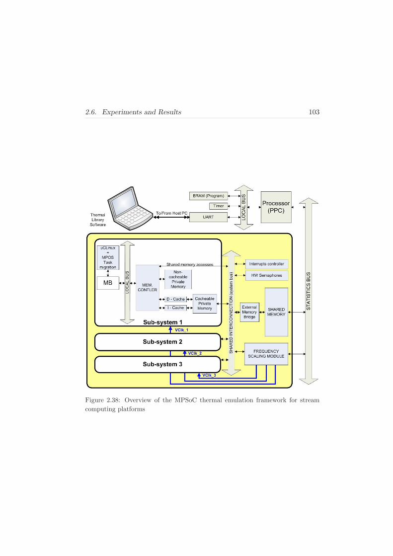
2.6. Experiments and Results 103
Figure 2.38: Overview of the MPSoC thermal emulation framework for stream
computing platforms

104 Chapter 2. Thermal Control Policies on MPSoCs
presented in [6] is the addition of a specialized thermal monitoring subsys-
tem, such that the run-time temperature of the emulated stream computing
platform can be observed at the MPOS level. This new monitoring subsys-
tem is based on hardware sniffers, a virtual clock management peripheral
and a dedicated non-intrusive subsystem, which implements the extraction
of statistics through a serial port. These statistics are provided to a software
thermal simulation library for bulk silicon chip systems [6], which resides in
a host workstation, and calculates the temperature of each cell according
to the floorplan of the emulated MPSoC and the frequency/voltage of each
Microblaze (MB) soft-core processor. Then, the temperatures coming out
from the simulator provide a real-time temperature information visible by
the running uClinux in each processor through emulated memory-mapped
temperature sensors, which are updated by the thermal monitoring sub-
system as configurable regular updates. In our experiments we have fixed
this updating interval to 10 ms to guarantee very accurate thermal mon-
itoring (see Section 2.6). Finally, thanks to a handshake mechanism be-
tween the thermal model and the MPOS middleware to synchronize the
upload/download of temperatures, our extended framework implements a
closed-loop thermal monitoring system, which enables exploring the im-
pact of task migration and scheduling on system temperature balancing at
multi-megahertz speed, and the observation of the real thermal transients
of MPSoC stream platforms.

2.6. Experiments and Results 105
2.6.2 Stream MPSoC Case Study
We focus on a homogeneous architecture, as presented in Figure 2.37. In
particular, we consider a system based on three 32-bit RISC processors
without MMU support to access cacheable private memories, and a single
non-cacheable shared memory. It follows the structure envisioned for non-
cache-coherent MPSoCs [89, 97]. In Table 2.2, we summarize the values
used for the components of our emulated MPSoC. The power values have
been derived from industrial power models for a 90nm CMOS technology.
On the software side, each core runs its own instance of the uClinux OS [73]
in the private memory (see Sections 2.2 and 2.3 for more details about the
MPOS software infrastructure).
Table 2.2: Power of components in 0.09 µm CMOS
Max. Power@500 MHz
RISC32-streaming (Conf1) 0.5W (Max)
RISC32-ARM11 (Conf2) 0.27W (Max)
DCache 8kB/2way 43mW
ICache 8kB/DM 11mW
Memory 32kB 15mW
We considered two different packaging solutions. The first package
shows temperature variations of around 10 degrees in few seconds [35],
while the second packaging option shows similar thermal variations in less
than a second. In Table 2.3 we enumerate the main thermal properties of

106 Chapter 2. Thermal Control Policies on MPSoCs
these two different packaging options. Regarding package-to-air resistance,
since the amount of heat that can be removed by natural convection in
MPSoCs strongly depends on the environment (e.g., placement of the chip
on the PCB), we have tuned these figures according to the experimental
figures measured in our industrial 3-core case study [35] and according to
the final MPSoC working conditions indicated by our industrial partners.
Table 2.3: Thermal properties of the different packages
silicon thermal conductivity 150 ·(
300
T
)4/3W/mK
silicon specific heat 1.945e− 12J/um3K
silicon thickness 300um
copper thermal conductivity 400W/mK
copper specific heat 3.55e− 12J/um3K
copper thickness 1000um
package-to-air conduct. (low-cost) 12K/W
package-to-air conduct. (high-cost) 1K/W
2.6.3 Benchmark Application Description
We ported to our emulation framework different multi-task variations of
the Software FM Defined Radio (SDR) benchmark (Table 2.4), which is
representative of a large class of streaming multimedia applications. The
application model follows the Streamit application benchmarks [1], used as
baseline for the implementation of our parallel SDR versions. This class

2.6. Experiments and Results 107
of applications is characterized by tasks communicating by means of FIFO
queues, as depicted in Figure 2.39, where tasks are graphically represented
as blocks. As this figure shows, the output data of the tasks of the SDR
application is stored in different buffers or queues (Qx,y) and consumed at
the required frame rate. Thus, a deadline miss occurs when the consumer
(periodically) attempts to read a frame from the final buffer and it is empty.
Figure 2.39: SDR case study (six tasks version)
We performed two sets of experiments. In the first set we used a very
dynamic workload made of multiple instances of the SDR application, using
versions divided in three or six tasks (as in Figure 2.39). The input data to
the SDR application represents samples of the digitalized PCM radio signal
to be processed in order to produce an equalized base-band audio signal. In
the first step, the radio signal passes through a Low-Pass-Filter (LPF) to
cut frequencies over the radio bandwidth. Then, it is demodulated by the
demodulator (DEMOD) to shift the signal at the baseband and produce
the audio signal. The audio signal is then equalized with a number of

108 Chapter 2. Thermal Control Policies on MPSoCs
Band-Pass-Filters (BPF) implemented with a parallel structure. Finally,
the consumer (Σ) collects the data provided by each BPF and makes the
sum with different weights (gains) in order to produce the final output.
Communication among tasks is done using message queues.
2.6.4 Evaluated State-of-the-Art Thermal Control Policies
MiGra has been compared with the following state-of-the-art thermal man-
agement policies:
Energy-Balancing: This policy maps the tasks of the SDR applica-
tion to balance their energy consumption [10] among the cores. Energy is
computed from the frequency and voltage imposed by the running tasks,
which are dynamically adjusted using DVFS [27].
Stop&Go: This policy prevents thermal runaway by shutting down
a core when it reaches a panic temperature threshold. In its original ver-
sion [19], the core execution is resumed after a predefined timeout. However,
we modified this policy to fairly compare it with our thermal balancing al-
gorithm, MiGra, by using the upper threshold of our algorithm as the panic
threshold, and our lower threshold defines when to switch the core on in-
stead of a fixed timing out value, which would be unable to adapt to very
dynamic working conditions.
Rotation: This policy tries to achieve thermal balancing by performing
migrations between cores in a rotatory fashion, at regular intervals. Thus,

2.6. Experiments and Results 109
at the beginning of a task migration interval (i), a set of tasks in corej is
migrated to core(j+1)modN .
Temperature-Based (TB): This policy considers the migration of
tasks between cores according to the temperature differences between each
pair of processing cores in regular intervals, namely, the set of tasks running
on the hottest core is swapped with the set on the coldest core, the set of
tasks on the second hottest core is swapped with the one on the second
coldest core, etc. Thus, at the beginning of each task migration process,
the cores are ordered by temperature. Then, the set of tasks executed on
corej is swapped with the set running on coreN−j−1.
Temperature-Based Threshold-limited (TB-Th): This policy is
an enhancement of the previous TB policy, which was originally aimed to
reduce peak temperature rather than thermal gradients. Therefore, we have
introduced an additional minimum temperature threshold, which tries to
minimize the number of unnecessary migrations of the original TB approach
between cores when the worst temperature of the MPSoC has not reached
a critical point. The minimum threshold has been carefully selected off-line
to find the best option for each working condition of our sets of experiments.
In the following sections we assess the performance of MiGra with respect
to the previously described policies in different workload conditions and for
different types of packaging solutions in stream computing platforms.
110 Chapter 2. Thermal Control Policies on MPSoCs
2.6.5 Experimental Results: Exploration with Different Pack-
aging Solutions
We compare MiGra, Stop&Go and the more classical energy balancing task-
migration policy, currently implemented in many MPOSes, using a low-
and high-cost thermal package. In addition, DVFS was always active at
the MPOS level to adjust the power dissipated by each core to the required
workload.
D.1) Thermal Balancing in a Low-Cost Packaging MPSoC: In the case
of low-cost packaging, we observed that after a first execution phase (12.5
sec), the temperatures of the three cores stabilizes. However, it is not bal-
anced and approximately 100C difference exists between the hottest (core
1) and the coolest core (core 3). This thermal state is due to the applica-
tion of DVFS to each core. Moreover, although core 2 and 3 have the same
frequency, their temperatures differ because of the different heat spreading
capabilities due to their position in the floorplan (see Figure 2.37). Thus,
in our experiments, we trigger our task-migration-based policy (MiGra) to
achieve thermal balancing after this initial phase.
When MiGra is applied, each time a core reaches the upper threshold
(set to three degrees more than the average temperature), a migration is
triggered, one task is moved to a colder core, and the temperature becomes
balanced for all cores within 1 second of execution of the SDR applica-

2.6. Experiments and Results 111
Table 2.4: Application mapping
Core / freq. Task Load [%]
Core 1 (533 MHz) BPF1 36,7
DEMOD 28,3
Core 2 (266 MHz) BPF2 60,9
Σ 6,2
Core 3 (266 MHz) BPF3 60,9
LPF 18,8
tion. This demonstrates the effectiveness of our policy to balance tem-
perature.Our results indicate that the hottest core temperature passes the
upper threshold while balancing the temperature only for a very limited
time (less than 400 ms).
A quantitative evaluation and comparison between our thermal-balancing
policy (MiGra), Stop&Go and energy balancing algorithms is provided in
the following experiments for the same packaging configuration. Figure 2.40
shows the temperature standard deviation for the three policies as a func-
tion of the threshold values. The X-axis indicates the distance of upper
and lower threshold from the mean temperature. As this figure shows, the
temperature deviation increases with the threshold. Thus, our policy is
more effective in reducing temperature deviation than other techniques be-
cause it acts on both hot and cold cores. In particular, the manually-tuned
Stop&Go does not improve the temperature of the cold cores. Furthermore,

112 Chapter 2. Thermal Control Policies on MPSoCs
if the original Stop&Go is used [19, 27], considering the highest-supported
temperature for the low-cost package as panic threshold, higher tempera-
ture swings are observed, which leads to a worst standard deviation value
(3.70˚K more) with respect to those shown in Figure 2.40.
� � � �
���
����
����
����
���
����
����
����
���
����
����
����
���
����
����
� ������������ ���
� ���������
�����������������������
&���� �������������'���
���!�����"#$%
! ������������ ����"#$%
Figure 2.40: Temp. standard deviation in low-cost embedded SoCs from the mean
on-chip temperature (337˚K)
Then, Figure 2.41 shows the number of deadline misses as a function
of the threshold values. As shown, our policy leads to few deadline misses
while Stop&Go suffers a higher value of missed frames. Deadline misses
may be caused by frozen tasks during migration; hence, inter-processor
queues are depleted during migration, and if the queue of the last stage
gets empty a deadline miss occurs. However, as Figure 2.41 illustrates,

2.6. Experiments and Results 113
migration is lightweight and fast enough to limit this drawback. In fact,
missed frames appear only for the minimum threshold considered in our ex-
periments. Furthermore, we observed that the average queue level does not
change because of migration; thus, a queue size handling thermal balancing
can always be found and the SDR application can sustain thermal balanc-
ing without QoS impact, i.e., the minimum queue size to sustain migration
in our experiments was 11 frames.
� � � �
�
�
�
�
��
��
��
��
��
��
��
��
����������
���������� ������ ��
������������ !
��� ��� �����"!
Figure 2.41: Deadline misses for the embedded mobile system
D.2) Thermal Balancing in High-Cost Packaging MPSoCs: To stress
our policy when temperature variations are faster, we repeated the pre-
vious set of experiments using the alternative packaging values for high-
performance systems (see Section 2.6.2), where temperature variations are

114 Chapter 2. Thermal Control Policies on MPSoCs
� � � �
����
����
����
����
����
����
����
����
����
����
����
���������
��� �����������������
��� ������������������
� ������� !"#
�
�� �
�����
���� !"#
Figure 2.42: Standard deviation in high-performance SoCs from the mean on-chip
temperature (314˚K)
six times faster than the previous model. Hence, the 3-core case study ex-
periences gradients of more than ten degrees, i.e, the coolest core typically
operate at 56˚C and the hottest one can reach 67˚C.
Figure 2.42 shows the standard deviation of the temperature for the
three tested policies. The energy balancing policy achieves very poor re-
sults and the modified Stop&Go policy behaves better in terms of tem-
perature deviation, but it causes a large amount of deadline misses (Fig-
ure 2.43). Morover, using the original version of Stop&Go [27] with the
highest-supported temperature of the high-performance package as panic
threshold, a worst standard deviation value of 4.48˚K more is observed

2.6. Experiments and Results 115
with respect to Figure 2.42.
On the contrary, although our algorithm makes temperature oscillate
more than the modified Stop&Go (but significantly less than the origi-
nal Stop&Go), it always causes very few deadline misses (less than 4%).
Moreover, our algorithm starts behaving noticeably better than Stop&Go
when the threshold increases, as less migrations are triggered. Also, we
observed that Stop&Go causes less deadline misses with the fast thermal
model than with the slow one, due to the faster speed the lower threshold
is reached after shutdown. From these experiments, we can conclude that
pure software techniques cannot handle fast temperature variations, and a
hardware-software co-design approach is needed.
� � � �
�
�
�
�
�
��
��
��
��
��
�� �������
�����������
����� ��� ��������� ���
������ ���� !"
��� ����
������#"
Figure 2.43: Deadline misses for high-performance systems

116 Chapter 2. Thermal Control Policies on MPSoCs
Finally, Figure 2.44 depicts the average number of migrations per sec-
ond performed by our thermal balancing policy (MiGra) for both mobile
embedded and high-performance systems. As expected, the number of
migrations is higher for high-performance systems. However, as each mi-
gration implies a transfer of 64 Kbytes of data (the minimum memory
space allocated by the OS), the required three migrations per second are
equivalent to 64 ∗ 3 = 192 Kbytes per second, which means that our task
migration policy implies only a negligible overhead in system performance
(1% overall).
2.6.6 Experimental Results: Limits of Thermal Balancing
Techniques for High-Performance MPSoCs
In this set of experiments we perform evaluation of the limits of MiGra and
state-of-the-art task migration policies, i.e., Rotation, TB and TB-Th (see
Section 2.6.4 for more details). In all the cases, local DVFS is also active
and applied, when possible, in addition to each particular task migration
scheme. To stress the reacting capabilities of all these schemes, in this set
of experiments we have used the high-performance packaging option, which
exhibits faster vertical on-chip heat flow dissipation to the environment than
spreading horizontally to other parts of the chip. Thus, even more dynamic
and faster thermal imbalance situations occur, because the different parts
of the system heat and cool down faster, as shown in our previous set of

2.6. Experiments and Results 117
experiments.
Then, we have evaluated and compared the behavior of the task migra-
tion algorithms under three different workloads, made of multiple instances
of the SDR case study, which was divided in three internal subtasks for
more accurate control of the final workload conditions. In the first work-
load setup we analyze the behavior of the different task migration policies
in the context of a steady-state thermal situation, where there is essentially
no thermal imbalance. Thus, the workload of each task was adjusted to
make deterministic the replication of load ratio among cores for the tested
thermal balancing policies, using a 65% workload approximately for each
processor. To this end, we partitioned the SDR case study in three tasks
having very similar processor workload requirements. Therefore, in this
situation, the processors tend to run at the same frequency. Next, in the
second workload setup we performed an uneven partitioned of the workload
between the three internal tasks that compose each SDR application. Thus,
the processors need to run at different frequencies and with variable num-
ber of memory and I/O operations, which results in a clear overall system
thermal imbalance. In particular, we used 55%-85%-30% workload at 35
frames/second for cores 1, 2 and 3, respectively. Finally, in the third work-
load setup, we assess the capabilities of MiGra to adapt to very dynamic
workloads by varying the frame rate of the SDR case study, and compare
this behavior against an offline-tuned version of the TB-Th migration pol-
icy. Thus, in this final setup, we obtained a workload of 46%-74%-26%,

118 Chapter 2. Thermal Control Policies on MPSoCs
55%-85%-30% and 58%-95%-33% for the frame rate interval using 30, 35
and 40 frames/sec, respectively.
� � � �
����
����
����
����
����
����
����
����
����
����
����
����
����
����
�������������
����������� ���
������������ !
��� ����"�
Figure 2.44: Migrations/sec of MiGra for both types of packages
For each setup we performed various experiments while exploring differ-
ent values of the internal configuration parameters of each policy, namely,
for MiGra we changed the threshold ranges, for Rotation and TB we mod-
ified task migration timeout values, and for TB-Th we varied its minimum
temperature unbalance threshold to force the migration process.
E.1) Setup I: Steady-State Thermal Context: Table 2.5 summarizes the
experimental results obtained for the first workload setup, where the tem-
peratures of the three cores are already in a steady-state situation. As

2.6. Experiments and Results 119
this table shows, the Rotation and TB policies are not effective, because
they try to swap tasks between the different cores without knowledge of
the overall temperature gradient across the chip. As a consequence, in
highly-demanding working conditions (with small timeouts to apply task
migration), both policies show a significant decrease in QoS of the target
3-core platform (i.e, 27% of deadline misses for Rotation and 13% for TB),
as they generate a large number of migrations. Conversely, MiGra and TB-
Th avoid migrations completely, since MiGra is able to observe that the
standard deviation of the temperature of the cores is within the allowed
temperature oscillation range, and also TB-Th does not react because we
have manually set up the minimum migration detonation threshold to val-
ues that are never reached by any processor.
Table 2.5: Experimental results for Setup I: Temperatures balanced (steady-state
thermal condition)
MiGra Rotation TB TB-Th
Timeout (ms) 10 10 10 20 10 20 10 10
Threshold (˚C) 2 1 316˚K 318˚K
Standard deviation 0 0 0.18 0 0.16 0 0 0
Deadline misses (%) 0 0 27.64 0 13.12 0 0 0
Migrations. / sec 0 0 30.47 15 20.48 10.00 0 0
E.2) Setup II: Unbalanced Thermal Gradients at Regular Intervals: Ta-
ble 2.6 depicts the experimental results obtained in the context of the second

120 Chapter 2. Thermal Control Policies on MPSoCs
workload setup, where the 3-core MPSoC platform under study experiences
thermal gradients, but in regular intervals, due to the unbalanced partition-
ing (but regular overall streaming computation workload) of the tasks. As
this figure shows, MiGra requires only a linear increase in the number of
migrations when we sweep the required threshold of average temperature
between the cores from four and one degree around the average temperature
of the platform. Moreover, it can be observed that the standard deviation
gradually increases, as the policy starts getting closer to the critical thresh-
old or reachable thermal balance limit for the studied 3-core MPSoC (i.e.,
less than one degree oscillation beyond/below the average temperature),
which is due to the unavoidable cost of migrating a certain task between
two cores. Nonetheless, even in the smallest range of requested thermal bal-
ancing, MiGra never experiences deadline misses, as it computes the global
benefits of each migration in the overall thermal balance of the MPSoC.
Then, if we compare the results of MiGra with the other task migration
policies, Table 2.6 shows that Rotation has always worst standard deviation
and requires many more migrations to compensate the thermal unbalance
of the MPSoC. Furthermore, if a very fine-grained timeout is requested
to Rotation, it degenerates and shows a very significant decrease in QoS,
namely, 26% of deadline misses on average. With respect to the TB pol-
icy, the experimental results show that it performs better than Rotation
by having a lower standard deviation in critical thermal balancing con-
straints, but the values are only marginally better than MiGra (0.10 versus

2.6. Experiments and Results 121
0.17). Nonetheless, this values are achieved by TB at the cost of a large
percentage of deadline misses (i.e., 7.62%) and QoS degradation, due to its
large amount of required task migrations to balance the overall tempera-
ture, while MiGra does not generate any deadline miss. Finally, although
TB-Th shows a lower number of deadline misses (1.62%) than TB or Ro-
tation in the most fine-grained threshold temperature to detonate a task
migration (316˚K), it still has deadline misses and experiences a larger
standard deviation than MiGra.
Table 2.6: Experimental results for Setup II: Temperatures unbalanced with reg-
ular workload cycles
MiGra Rotation TB TB-Th
Timeout (ms) 10 10 10 20 10 20 10 10
Threshold (˚C) 2 1 316˚K 318˚K
Standard deviation 0.17 0.22 1.57 0.99 0.10 0.37 1.76 0.49
Deadline misses (%) 0 0 26.23 0 7.62 0 1.62 0.00
Migrations/ sec 5.89 8.07 30.25 14.98 19.94 9.98 12.02 8.51
E.3) Setup III: Highly-Variant Thermal Gradients at Irregular Intervals:
In this last setup we have evaluated the ultimate reaction capabilities of
MiGra to highly-dynamic workloads (i.e., variable frame rates in stream
computing), which generate thermal gradients at very variable intervals.
Furthermore, we have compared its behavior with respect to the best TB-
Th configuration decided off-line as the best intermediate value for the SDR
benchmark with different frame rates, after analyzing the thermal gradients

122 Chapter 2. Thermal Control Policies on MPSoCs
derived from the execution of the application on the target 3-core MPSoC.
As a result, we manually defined the minimum migration threshold value in
TB-Th as 318-degree K, see Table 2.6, and compared it with a fine-grained
configuration threshold for MiGra (i.e., a threshold of 2 degrees around the
average temperature). Then, we evaluated both policies using three frame
rates: 30, 35 and 40 frames/sec.
Table 2.7 summarizes the results. On one hand, this table shows that
the numbers of migrations required by MiGra to guarantee the requested
thermal balancing of less than 3 degrees at 30 frames/sec is very limited,
although it is a valid frame rate for many stream computing applications.
This limited number of migrations is due to the fact that at this frame rate,
the workload of each task is below 50% for the 3-core platform under study.
Thus, MiGra can effectively work and adapt the global thermal behavior of
the system very fast by mapping two tasks in the same processing core at
each moment in time, if this value can reduce the global energy of the system
and balance the temperature, as indicated in the constraints of MiGra (cf.
Section 2.5.1). Conversely, for 35 or 40 frames per second, the processors
are always loaded more than 50%. Thus, several migrations are required to
dynamically balance and swap one of the tasks between processors. Hence,
MiGra performs about double number of migrations with input rates higher
than 30 frames/sec, as it is shown in Table 2.7. Then, the differences in
the number of migrations between 35 or 40 frames per second are not very
significant for MiGra, no deadline misses exists, and the standard deviation

2.6. Experiments and Results 123
can be well-adjusted to each case.
Table 2.7: Experimental results for Setup III: MiGra vs. TB-Th in a highly-variant
thermal gradient context
MiGra TB-Th
Frame Rate (per sec) 30 35 40 30 35 40
Standard Deviation 0.27 0.12 0.04 0.15 0.49 0.10
Deadline Misses (%) 0 0 0 0 0 0
Migrations/ sec 2.49 4.62 4.42 3.17 8.51 2.74
On the other hand, TB-Th always swaps the tasks between the hottest
and the coldest processors, without a complete knowledge of the influence
of workload in the overall number of migrations, since it is not possible
to define a minimum task migration threshold that works correctly for
all possible variable working conditions. Therefore, this policy can create
very anomalous conditions for some variable workloads, as it is the case
of 35 frames/sec (see Table 2.7), where a large number of migrations are
suddenly necessary to compensate for peaks of workloads accumulated in
some processors. Indeed, in some cases, TB-Th reacts inappropriately to
the gradient trends of parts of the MPSoC, as the minimum migration
threshold defined in this policy cannot be dynamically changed. As a result,
if a task migration timeout occurs for TB-Th before the last migration of
a task from a hot core to a cold one has finished, as the system is beyond

124 Chapter 2. Thermal Control Policies on MPSoCs
the minimum threshold to detonate new migrations, TB-Th can trigger a
new migration phase that brings back more workload to the hot processing
core, raising its temperature again. As a consequence, TB-Th performs
an unnecessary number of migrations in certain situations with highly-
dynamic workloads, and the perfect adjustment of its internal parameters
is critical for a good behavior of this policy. Nonetheless, these highly-
dynamic workloads are very difficult to predict at design time in order to
suitably tune the thresholds and timeouts of the TB-Th algorithm for each
target MPSoC.
Conversely, MiGra is only slightly affected by variable workloads, due
to its fast run-time self-adaptation of the upper and lower thermal-based
task migration thresholds. Thus, it can adapt to the thermal dynamics of
each target MPSoC, and the standard deviation and number of deadline
misses are largely insensitive to initial internal parameters tuning. Hence,
it is easier to tune to any final MPSoC architecture.
2.7 Conclusions
As chip component sizes decrease, power dissipation and heat generation
density exponentially increase. Thus, temperature gradients in MPSoCs
can seriously impact system performance and reliability. Thermal balancing
policies based on task migration have been proposed to modulate power
distribution among processors to achieve temperature flattening. However,

2.7. Conclusions 125
in the context of MPSoC stream computing, the impact of migration on
quality of service must be carefully studied.
Here we have presented a new thermal balancing policy, i.e., MiGra,
specifically designed to dynamically exploit workload information and run-
time thermal behavior of stream computing architectures. MiGra keeps
migration costs and deadline misses bounded to reduce on-chip tempera-
ture gradients via task migration. Besides, it supports the application of
local DVFS schemes, that work independently. We have thoroughly evalu-
ated the potential benefits of MiGra to balance the temperature in stream
processing architectures with respect to state-of-the-art thermal manage-
ment techniques using different versions of a software-defined radio multi-
task benchmark. We have run dynamic workloads of this benchmark on
a complete cycle-accurate FPGA-based emulation infrastructure of a real-
life 3-core stream platform, and the experimental results show that MiGra
is able to reach a global thermal balance where the temperatures of the
MPSoC components are within a range of 3 degrees around the average
temperature. Furthermore, MiGra achieves this thermal balancing with a
negligible performance overhead of less than 2% in MPSoC stream comput-
ing platforms, significantly less than state-of-the-art thermal management
techniques.
This work has been presented at DATE 2008 conference and then pub-
lished as a conference proceeding [67]. A further extension, much more
detailed, has been published in a journal [66]. This also contains, with re-

126 Chapter 2. Thermal Control Policies on MPSoCs
spect to the conference version, new evolutions, experiments and results.
Chapter 3
Energy-Constrained Devices:
Wireless Sensor Networks
Wireless sensor networks (WSN) are largely utilized in many fields and are
going to experience a much more diffusion in the near future. A WSN con-
sists of spatially distributed autonomous sensors that cooperatively monitor
physical or environmental conditions, such as temperature, sound, vibra-
tion, pressure, motion or pollutants. Currently they are used in many indus-
trial and civilian application areas, including industrial process monitoring
and control, environment and habitat monitoring, healthcare applications,
home automation and traffic control. WSNs often deeply rely on batteries
as the only source for their normal operations. In many situations, espe-
cially when sensors are spread over large areas (as forests) to be monitored,

128 Chapter 3. Energy-Constrained Devices: Wireless Sensor Networks
their lifetime is strictly bounded with that of their energy source, that is,
their battery. Often it is not economically convenient to change (or charge)
the batteries, even if possible at all: sometimes sensors are diffused in the
territory launching them from a plane, for example. Energy consumption
hence is a serious concern, proportional to how costly it is charging the bat-
teries. As such, techniques to tame energy consumption and extend sensors
lifetime are essential to reduce deployment and operating costs.
Today’s sensor nodes can be equipped with powerful microcontrollers
to address the increasing need of real-time processing of sensed data. For
instance, body sensor networks for gesture recognition require filtering of
acceleration values at line rate. This requirement imposes a paradigm shift
with regard to more traditional sensor networks characterized by low activ-
ity duty cycles. Therefore, energy conservation strategies applied to wireless
sensor nodes to increase their lifetime must take into account computation
power rather than focusing only on communication power. In this chapter
I present a novel approach which aims at exploiting the knowledge of net-
work status to optimize the power consumption of the node microcontroller.
The proposed approach has been tested in various network conditions, both
synthetic and realistic, in the context of IEEE 802.15.4 standard. Exper-
imental results demonstrate that the proposed approach allows to achieve
power savings of up to 70% with minimum performance penalty.
This work has been published in [65] and a journal edition is currently
under peer review.

3.1. Introduction 129
3.1 Introduction
Wireless sensor networks (WSN) have recently gained more and more at-
tention in human computer interaction (HCI) and e-health applications
for gesture recognition and body posture monitoring. In these applica-
tions, sensor nodes elaborate data from body mounted accelerometers or
gyroscopes to reconstruct movements. Hence, node’s microcontroller must
perform integrations or trigonometric function computations in real-time.
As a consequence, the power consumption of the processing components of
the node is much higher (i.e. imposing a duty cycle of 50% or more) than
in traditional WSN applications such as infrastructure monitoring or video
surveillance where activity duty cycles of nodes are on the order of 1%.
As a consequence, a paradigm shift in the design of energy management
strategies for wireless sensor networks is required, where management of
microcontroller’s energy plays a central role together with communication
energy reduction.
Figure 3.1 depicts a typical data flow in a sensor network application.
The producer node acquires data by using its sensors, then it processes
data by using a microcontroller and puts results in the transmission queue
to be sent over the network. These operations must be performed at the
proper speed to match application performance requirements. Tradition-
ally, in wireless transmissions, packet reception is confirmed by sending
back an acknowledgment. If the quality of the radio link is poor or the

130 Chapter 3. Energy-Constrained Devices: Wireless Sensor Networks
receiver cannot receive data then no ack comes back and the packet is kept
in the queue to be retransmitted. Furthermore in contention-based access
protocols (e.g., the IEEE 802.15.4 [58]) the packet transmission is delayed
if the channel is busy. As a consequence, at the producer side the trans-
mission queue may become full thus wasting CPU power. Indeed, the data
processed by the microcontroller will be either discarded before entering
the queue (drop tail policy) or will cause the dropping of packets in the
head of the queue (drop head policy). Independently from the dropping
policy (for which we do not make any assumption here), since typically
the size of the transmission queue is small (16 to 32 packets), most of the
data processed by the microcontroller will be lost in case of relatively long
network congestion conditions. This means that in such cases it is more
convenient to slow-down processing speed and save microcontroller’s power.
We consider long periods as those leading to transmission queue overflow.
This means that congestion periods smaller than the time needed to fill in
the transmission queue do not cause the activation of our speed slow-down
policy.
The efforts done in the past to decrease energy spent in transmis-
sion/reception and the increasing role of computation in today’s applica-
tions have made CPU power consumption more critical for node’s power
budget. It has been shown that the CPU is one of the most consuming
components of a modern wireless sensor node ([44], [82]). In particular [82]
performed a very accurate profiling of energy consumption of the widely

3.1. Introduction 131
Figure 3.1: Data flow in a sensor network application
adopted Mica2 sensor node. Their results show that the CPU power con-
sumption ranges from 28% to 86% of the total power consumed and roughly
50% on average. Moreover, depending on the node application domain, fur-
ther activity can be assigned to the CPU (i.e. data filtering), thus raising
its power consumption share.
Several energy management approaches aiming at optimizing network
lifetime have been proposed in the past (see [23] for an overview); most
of them focus on communication power reduction [85, 107]. Concerning
processing power, recent works exploit topology and communication range
optimization to shutdown the cores [52, 61, 100]. A distributed power man-
agement approach is presented in [108] where coordination among nodes
aims at optimizing the timeout of their sleeping periods. Route and net-
work activity information is exploited in [99] to decide when to turn the
node into the sleeping status. Other works investigated Dynamic Frequency
Scaling (DFS) and Dynamic Voltage Scaling (DVS) [83] to reduce power
consumption when the CPU is in idle state.

132 Chapter 3. Energy-Constrained Devices: Wireless Sensor Networks
The limit of those approaches is that they do not exploit the knowl-
edge of network conditions to save power. In this chapter I present a novel
approach where network information is exploited to independently adapt
the processing rate of each sensor node to network conditions. Since WSN
protocol stacks lack of rate-control algorithms such as those implemented
in TCP, the occupation of MAC queue has a linear relationship with the
difference between application production rate and network consumption
rate. For this reason, we implemented our network-adaptive approach di-
rectly at MAC level. Nevertheless, we believe the proposed policy could be
applied also in presence of rate-control protocols by appropriate tuning of
the control law.
To adapt the processing rate to the network condition a control strategy
has been designed and implemented, that must satisfy conflicting objec-
tives. From one side, it must be reactive enough to detect network conges-
tion conditions early enough to: i) allow power saving when the queue is
filling up, and ii) to avoid queue depletion that would compromise quality
of service. On the other side, large reactivity will lead to frequent speed
switchings, that are not desirable because of their time overhead (which is
taken into account in our experiments). We studied a non-linear control
approach that is able to address these objectives. We implemented it on
a power-aware wireless sensor network simulator that models a network
of TI CC2430 nodes, each consisting of a processing core and a radio in-
terface running the 802.15.4 MAC layer. To evaluate the effectiveness of

3.2. Computation Energy Management 133
the proposed strategy, we performed experiments using a realistic human
body monitoring application case study to detect real network congestion
conditions.
This chapter is organized as follows: Section 3.2 explains the energy
management strategy, Section 3.3 describes the target platform and mod-
eling approach while Section 3.4 describes the experimental results. Sec-
tion 3.5 concludes the work.
3.2 Computation Energy Management
Modern microcontrollers support various operating clock frequencies
that can be programmed by the software applications through a dedicated
API. Typically, these frequency values are obtained by dividing the max-
imum frequency by a factor of two. Indeed, frequency scaling is obtained
by a pre-scaler hardware module acting on the clock signal entering the
microcontroller core. The clock scaling can be exploited by an energy man-
agement policy to save power when the production of new packets would be
useless since packet transmission slows down and the transmission queue
is getting full. This fact happens when the channel is busy, the quality of
the radio link is poor (e.g., due to interference, path loss, obstacles) or the
receiver is sleeping or overloaded. In this case, the processing speed can
be decreased until packet transmission rate increases again. Therefore, the
transmission queue can be used to monitor the network status.

134 Chapter 3. Energy-Constrained Devices: Wireless Sensor Networks
When the network quality is low, the transmission queue of a node starts
filling-up at a speed depending on the producer rate (the microcontroller)
and, if the condition persists, it can become full. Thus, to save power on
the microcontroller, a simple approach could be to switch to the lowest
possible frequency value (or even shut-off) when the transmission queue
becomes full and restore the maximum frequency when the queue starts
to be depleted again. We called this simple algorithm On-Off (OO) and
let set-point be the level of the queue which triggers frequency change. A
more aggressive approach would be to reduce the processor speed before
the queue is full (i.e., using a lower set-point) to save more power. However,
there are two side effects from the performance viewpoint. First, the average
queue level is lower, which implies that there could be less packets to be
transmitted once the congestion period finishes. That could worsen the
quality of service. Second, if the algorithm is not reactive enough, the
processor speed at the end of the congestion period could be lower than
the maximum, thus leading to a lower transmission rate on average (again
a QoS worsening). As such, there is a trade-off between power saving and
performance that should be explored during the design of the control rule.
To implement a more aggressive approach with a limited impact on
performance, we explored the use of a non-linear feedback control which
has been developed in the field of multiprocessor systems to regulate the

3.2. Computation Energy Management 135
P C
Q
fP
fC
kP
kC
Figure 3.2: Producer (P) / Consumer (C) architecture
speed of a pipeline of cores [18].
3.2.1 Non-linear Feedback Control
In this section we describe our proposed non-linear speed scaling technique,
namely HQ. Let us derive a dynamical model of the two-stage producer-
consumer architecture represented in Figure 3.2. In our system the micro-
controller (producer) inside the node produces data that are injected in the
transmission queue of the node network interface (consumer). Let Q be the
occupancy of the transmission queue (by definition, Q is an integer non-
negative number) and fP be the producer clock frequency. The network
consumption rate fC is an external constraint. This rate is time-varying
and depends on network conditions.
Denote as kP fP the data rate of the producer processor, and let kCfC

136 Chapter 3. Energy-Constrained Devices: Wireless Sensor Networks
be the data rate of the consumer, with kP and kC being proper positive
gains. To facilitate system modeling and controller design, we define Q(t)
as a real-valued (i.e., “fluid”) approximation of Q, and we consider the
following dynamical model:
Q(t) = kP fP (t)− kCfC(t) (3.1)
where Q plays the role of the system output to control, fP is the user-
adjustable control input and fC represents an external disturbance term.
The frequency fP can take on values over a discrete set. Let Qcap be
the queue capacity and let Q∗ = Qcap/2 be a convenient set-point for the
queue occupancy.
Denote as follows the “error variable” e to be regulated.
e = Q−Q∗ (3.2)
The control algorithm 3 processes the current queue occupancy error
e[k] and its previously observed value e[k − 1].
Besides, we introduce a dead zone centered around the set-point where
the algorithm does not change the frequency and we denote it as 2∆ (by
definition ∆ is a non-negative integer). The dead zone has the purpose of
limiting frequency changes.
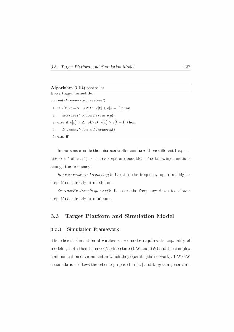
3.3. Target Platform and Simulation Model 137
Algorithm 3 HQ controllerEvery trigger instant do:
computeFrequency(queuelevel)
1: if e[k] < −∆ AND e[k] ≤ e[k − 1] then
2: increaseProducerFrequency()
3: else if e[k] > ∆ AND e[k] ≥ e[k − 1] then
4: decreaseProducerFrequency()
5: end if
In our sensor node the microcontroller can have three different frequen-
cies (see Table 3.1), so three steps are possible. The following functions
change the frequency:
increaseProducerFrequency(): it raises the frequency up to an higher
step, if not already at maximum.
decreaseProducerfrequency(): it scales the frequency down to a lower
step, if not already at minimum.
3.3 Target Platform and Simulation Model
3.3.1 Simulation Framework
The efficient simulation of wireless sensor nodes requires the capability of
modeling both their behavior/architecture (HW and SW) and the complex
communication environment in which they operate (the network). HW/SW
co-simulation follows the scheme proposed in [37] and targets a generic ar-

138 Chapter 3. Energy-Constrained Devices: Wireless Sensor Networks
chitectural template in which software (that will eventually run without
changes on the actual board) accesses one or more hardware devices that
have to be designed. This scenario maps onto a so-called ISS-centric co-
simulation model consisting of an instruction set simulator (ISS) running
the application and the operating system that interfaces through its drivers
to the hardware models specified by a hardware description language such
as SystemC [2]. The interaction between simulated software and hardware
modules is simplified by the fact that many embedded platforms support
memory-mapped HW access, i.e., CPU accesses external registers through
memory read/write operations. Therefore, the ISS is modified to redirect
read/write operations for specific addresses to the hardware simulation ker-
nel which updates the status of the corresponding HW modules.
The simulation infrastructure enables accurate power estimation thanks
to the following main features: i) timing synchronization between SystemC
model and ISS; ii) power annotation of CPU states and hardware compo-
nents [38]. To achieve effective evaluation of power management strategies,
power model of HW components has to support voltage and clock frequency
scaling as well as shutdown states. To this purpose, each hardware com-
ponent will be associated with a power state machine [11] and a power
consumption value will be associated to each state. Parametric states will
be also used for specific components for which the power consumption de-
pends on the voltage and clock frequency, such as the microcontroller. The
transitions among power states of SystemC modules will be controlled by

3.3. Target Platform and Simulation Model 139
the software running on the ISS through the dedicated power information
protocol as described in [38].
3.3.2 Network Model
To effectively simulate the wireless network to which sensor nodes are con-
nected, a SystemC collection of components has been created to reproduce
packet transfer over a radio channel [36]. In this way the same tool used to
simulate part of sensor nodes is seamlessly exploited to reproduce network
behavior, thus gaining simulation efficiency. Figure 3.3 shows the architec-
ture of the SystemC Network Simulation Library. White boxes represent
SystemC modules while gray boxes are pure C++ classes; black arrows
represent connections through SystemC ports; bold black arrows represent
inheritance and round edges denote relationships through object references.
Module Node t models a generic network node; it has three input ports
(generic input, network input, received signal energy input) and an output
port (network output). Module Node t has a set of properties which are
used by the simulation framework to reproduce network behavior. Nodes
have a state which can be running, off, or sleeping to save power. Transmis-
sion rate represents the number of bits per unit of time which the interface
can handle; it is used to compute the transmission delay and the network
load. The transmission power is used to evaluate the transmission range
and the signal-to-noise ratio. Node state, transmission rate and transmis-

140 Chapter 3. Energy-Constrained Devices: Wireless Sensor Networks
Figure 3.3: Architecture of the SystemC Network Simulation Library

3.3. Target Platform and Simulation Model 141
sion power can be changed during simulation to accurately simulate and
evaluate power saving algorithms. As shown in Figure 3.3, sub-classes of
Node t can be created to describe actual nodes. The sub-class specifies the
functional and timing behavior of the node (e.g., the CSMA/CA policy);
it can define additional ports and whether data sampling is triggered by a
change of the value on the data input port or scheduled by the node itself.
Instances of the module Timer t can be connected to user-defined nodes to
implement timed actions.
The data input port of each node can be bound to an instance of the
module Stimulus t which reproduces a generic environmental data source.
Class Network t is the core of the network simulator. It reproduces the be-
havior of the channel and manages the packet forwarding from the source
node to the destination nodes: transmission delay, path loss, collisions, and
the state of destination nodes are taken into account. Module NodeProxy
is the interface between nodes and the network and each instance of Node
must be bound to a different instance of NodeProxy. Each node interacts
with its own nodeproxy by using SystemC signals only, while nodeproxies
interact with Network t through object references. By using NodeProxy,
nodes can be designed as pure SystemC modules without object references
to other non-SystemC classes; this approach enables the use of traditional
hardware verification and synthesis tools. Exchanged packets are modelled
by the Packet t class which contains the address of source and destination
nodes, the packet length and a general-purpose payload field. Packet defi-

142 Chapter 3. Energy-Constrained Devices: Wireless Sensor Networks
nition can be changed since its fields are used by model-specific code while
only its size is used by the network; general purpose classes are indepen-
dent from the packet structure since it is specified through the template
mechanism.
3.3.3 Target Platform Model
This section describes the modeling of a wireless sensor node, called AquisGrain-
2 provided by Philips [29] and designed for body-worn smart medical sen-
sors. The main modules belonging to a sensor node based on the AquisGrain-
2 platform are the following: (I) ZigBee SW stack; (II) Intel 8051 CPU,
memory (ROM, RAM, flash) and I/O ports; (III) IEEE 802.15.4 RF transceiver;
(IV) Sensors/actuators. Figure 3.4 shows how the model of the AquisGrain-
2 is mapped onto the co-simulation framework. The ISS used to model the
Intel 8051 CPU is uCsim [28]. SystemC is used to model HW devices. The
overall HW/SW configuration consists of the following entities:
• SystemC RTL model of the accelerometer chip;
• SystemC RTL model of the UART/SPI device, which is attached to
an input/output port of the accelerometer to exchange data with the
CPU;
• C application retrieving data coming from the accelerometer and
sending them over the Network; this application is executed by using
uCsim;

3.4. Experimental Results 143
Figure 3.4: Co-simulation of the AquisGrain-2 node and of the wireless network
• SystemC model of the Network implemented through SCNSL.
3.4 Experimental Results
In this section we assess the effectiveness of the two feedback control power
management policies described in Section 3.2, namely OO and HQ. We also
compare them against the case in which there is not power management
(we called this last case NO); we evaluate the trade-off between obtained
power savings and quality of service impact. The policies are implemented
within the network interface driver of the sensor node, so that their cost
in terms of performance and power is taken into account. The benchmark

144 Chapter 3. Energy-Constrained Devices: Wireless Sensor Networks
consists in sampling acceleration values, performing a simple filtering op-
eration and sending them over the network. The acceleration sample rate
depends on the speed of the microcontroller, as shown in Table 3.1 where
the power consumption of the core at the various frequencies is reported
too. It is worth noting that in this benchmark, when the network is not con-
gested, the bottleneck is represented by the processing rate rather than the
network bandwidth. This is a typical situation for sensor network applica-
tions. As such, even at maximum speed, the transmission queue depletes.
Therefore, the feedback control strategy exploits the channel congestion
periods, that cause the saturation of the queue, to save the power spent
by the microcontroller. To show the dependency of the proposed approach
on network conditions, we modeled different network congestion patterns,
both synthetic and realistic. We represent the congestion interval length
as a fraction of the total transmission time. In Section 3.4.1 we consider
a coarse grained pattern with sporadic events of variable length. This
scenario emulates temporary disturbances such as a radio interference. In-
stead in Section 3.4.2 we consider a fine grained pattern, where congestion
intervals alternate to free intervals, shaping a periodic square wave with a
duty-cycle of 50%. In these experiments we vary the length of the wave
period. Finally, in Section 3.4.4 we model a real case scenario.
In all the experiments the transmission buffer length of the network
interface is set to 15 packets and the set-point (expressed as a fraction of
the buffer length) is fixed at 1/2 for the HQ and 14/15 for the OO. Each

3.4. Experimental Results 145
Table 3.1: Power vs performance characteristics of the microcontroller
Frequency Output Rate Power
8 MHz 2 KHz 8.25 mW
16 MHz 4 KHz 14.85 mW
32 MHz 8 KHz 31.35 mW
simulation ends after the transmission of a given amount of packets over
the network. In these experiments we focus on the microcontroller power.
As such, power consumption of the radio is not included. Note that there
is a negligible delay for changing the speed at run time being this obtained
by programming a pre-scaler placed on the clock path to the core.
To determine the impact on performance of the power management ac-
tions we consider the effective transmission rate, i.e., the number of packets
sent per time unit within time intervals free of congestion. Performance im-
pact must be compared, for the same channel conditions, against the NO
case (i.e., not power management), taking into account the obtained power
savings.
3.4.1 Coarse Grained Channel Congestion
The Figure 3.5 reports the power saving (with respect to NO) of one sensor
node over the channel congestion ratio (that is the congestion interval length
as a fraction of the total transmission time). It clearly shows that power
saving is proportional to the channel congestion ratio.
This is because longer the channel is busy, longer the frequency is held

146 Chapter 3. Energy-Constrained Devices: Wireless Sensor Networks
0
10
20
30
40
50
60
0 10 20 30 40 50 60 70 80
Channel congestion ratio (%)
Po
wer
savin
g (
%)
OO
HQ
Figure 3.5: Power saving (%) as a function of the channel congestion ratio
down. It is worth noting that we reached 50% of power saving in our best
setup, but it can reach higher values with higher channel congestion ratio,
up to the theoretical power saving upper limit of about 73%, obtained
by always keeping the frequency at its lower level. To better understand
these results, we can analyze the queue behaviour; Figure 3.6 shows the
queue length over time with different percentages of channel congestion and
without frequency scaling. It is possible to see that bigger the congestion
ratio, longer the queue stays full; if frequency scaling were active, bigger
the congestion ratio and longer the frequency would be held down.
We experimentally observed that for each case (NO, HQ, OO) the ef-
fective transmission rate is constant as a function of the channel congestion
ratio, but it has different values for each of them. With respect to NO, OO
impacts the performance of 2.6% and HQ of 6.5%. The HQ, being the more

3.4. Experimental Results 147
NO Algorithm
0
2
4
6
8
10
12
14
16
0 200000 400000 600000 800000 1000000 1200000 1400000
Time
Qu
eu
e le
ng
th
20%
50%
70%
Figure 3.6: Queue length over time without frequency scaling
aggressive, shows the worst performance value. On the other side, this is
compensated by the fact that it has the best power saving result (Figure
3.5). Conversely, being more conservative, the OO algorithm imposes a
smaller impact on performance but it is less effective from a power saving
viewpoint. Later in this section we will explore the trade-offs available by
configuring the parameters of these algorithms.
Figure 3.7 compares the level of the queue over time for the three al-
gorithms for a given percentage of channel congestion (20%). It is evident
that power management policies deplete the transmission queue due to the
frequency scaling on the microcontroller. Once the queue is empty, the
transmitter has to wait leading to a slow-down of the transmission rate
(QoS worsening).

148 Chapter 3. Energy-Constrained Devices: Wireless Sensor Networks
Algorithms comparison
0
2
4
6
8
10
12
14
16
0 50000 100000 150000 200000 250000 300000
Time
Qu
eu
e le
ng
th
NO 20%OO 20%HQ 20%
Figure 3.7: Comparison of queue occupancy as a function of time and with different
power management strategies
3.4.2 Fine Grained Channel Congestion
In this section, the chosen network conditions cause frequent changes in the
queue level, as shown in the two plots in Figure 3.10, thus offering a more
dynamic behavior to test the feedback policies. The effective transmission
rate for each algorithm is not constant anymore, but it decreases as the
congestion period length increases as shown in Figure 3.9. As with the
previous case, the HQ saves more power than OO (Figure 3.8), even if it
has a slightly higher performance impact (Figure 3.9).
It can be observed that at 50 ms of congestion period the effective
transmission rate is the same for all the algorithms. In this case the queue
always stays under the set-point (see Figure 3.10a), i.e., frequency scaling
is never triggered.

3.4. Experimental Results 149
0
5
10
15
20
25
30
35
0 50 100 150 200 250
Channel congestion period length (ms)
Po
we
r s
av
ing
(%
)
OO
HQ
Figure 3.8: Power saving as a function of the channel congestion period length
170
190
210
230
250
270
290
0 50 100 150 200 250
Channel congestion period length (ms)
Eff
ec
tiv
e t
ran
sm
iss
ion
ra
te
(packets
/s)
NO
OO
HQ
Figure 3.9: Effective transmission rate as a function of the channel congestion
period length

150 Chapter 3. Energy-Constrained Devices: Wireless Sensor Networks
0
2
4
6
8
10
12
14
16
0 200000 400000 600000 800000 1000000
Time
Qu
eu
e l
en
gth
50ms 100ms
0
2
4
6
8
10
12
14
16
0 200000 400000 600000 800000 1000000 1200000
Time
Qu
eu
e le
ng
th
150ms 200ms
Figure 3.10: Queue length over time without frequency scaling for congestion
length of: a) 50 ms and 100 ms; b) 150 ms and 200 ms
The results in Figure 3.9 show that the effective transmission rate de-
pends on the congestion period length. This can be justified by analysing
the queue occupancy over time depicted in the two plots in Figure 3.10.
For the sake of clarity, here we show only the case in which no power man-
agement is applied for different values of the period length (the behaviour
of the other algorithms is similar). Both plots refer to the transmission of
the same number of packets. It is worth noting that the falling edge of the
peaks is that of maximum transmission speed, because packets accumu-
lated in the buffer are consumed at the network rate after the congestion,
being not limited by the CPU speed. When congestion periods are small
such that the queue never becomes full, the effective transmission rate is
independent from the congestion period as expected because the sum of
intervals in which the queue is empty is constant. This is depicted in Fig-
ure 3.10a and it corresponds to congestion periods of 50 ms and 100 ms.

3.4. Experimental Results 151
On the other side, if the buffer saturates as shown in Figure 3.10b, the total
time in which the queue is empty becomes larger because the buffer does
not serve as packet reservoir. In practice, there are less opportunities to
transmit at higher rate exploiting the full buffer situation. This situation
holds also for congestion periods of 150 ms and 200 ms. From a power sav-
ing perspective, Figure 3.10b shows that by increasing the period length,
the queue keeps saturated for a longer time, giving more opportunities to
slow down the frequency. This is the reason why the power saving increases
together with the congestion length.
3.4.3 Parameters Tuning
By tuning some parameters of the algorithms it is possible to achieve a
variety of power/performance trade-offs. In particular, by changing the
set-point such that it corresponds to different fractions of the buffer length:
1/4, 1/2, 3/4 for the HQ and 1/2, 3/4, 14/15 for the OO. It must be
noted that it is not possible to compare the set-points between the two
algorithms, because they are used in a different way, as explained before.
Hence, we chose the above set-points observing the average queue level over
time, picking up the extreme values in the following manner:
• upper set-points (3/4 for HQ and 14/15 for OO): minimum value
(respectively for each algorithm) that causes an average queue level
equals to the NO case;

152 Chapter 3. Energy-Constrained Devices: Wireless Sensor Networks
• lower set-points (1/4 for HQ and 1/2 for OO): maximum value (re-
spectively for each algorithm) that causes an average queue level
equals to the case where the CPU frequency is held at minimum
level.
After that, we chose another value (for each algorithm) in the middle
(1/2 for HQ and 3/4 for OO). Furthermore, we performed these experiments
only for the fine grained case and at a given channel congestion period
length (150 ms).
In order to drive practical rules for parameter selection, we plotted the
Pareto optimal configurations in Figure 3.11, that highlights the achievable
trade-offs between energy saving and performance impact. Depending on
the application requirements, different configurations can be selected and
therefore different parameter settings. For instance, if a more aggressive
policy is needed at the price of a slightly higher performance penalty, the
HQ algorithm can be set to 1/4, which provides the highest power saving
and the worst effective transmission rate. Conversely, if the highest possible
QoS is required, the OO algorithm should be used with a set-point of 14/15.
3.4.4 Realistic Case Study
In order to test our algorithms in real life situations, we simulated a wire-
less sensor network in a car manufacturing industry, used to control the
activities of workers in the car assembly line. The sensors are placed on the

3.4. Experimental Results 153
20
21
22
23
24
25
26
27
28
120000 130000 140000 150000 160000 170000 180000 190000
Effective transmission time (us)
Po
wer
(mW
)
HQ
OO
14/15
3/4
1/2
3/4
1/2 1/4
Figure 3.11: Pareto optimal configuration for HQ and OO algorithms
body of workers to monitor their checking procedure (a full description of
this scenario is described in [109] and [88]).
We statistically reproduced the same transmission patterns of that sce-
nario in our simulator, using a two-state Markov chain to characterize the
transmission activity of each node. Figure 3.12 depicts the Markov chain;
in our case there are two states, named A and B, corresponding to a non-
transmission and transmission state, respectively. The transition probabil-
ity from the two states is regulated by α and β parameters obtained through
several realistic data traces taken from the scenario described above. When
the simulation begins, α and β parameter values are passed as parameters
to each instantiated node, so that they generate a network traffic statis-
tically similar to the realistic one. We performed several experiments by
varying the number of nodes of the network, to simulate various channel

154 Chapter 3. Energy-Constrained Devices: Wireless Sensor Networks
1-1- A B
Figure 3.12: Two-state Markov chain
congestion levels.
Figure 3.13 shows the results obtained on the realistic case study and
confirms that through network-aware speed control algorithms it is possible
to save a considerable amount of power (up to about 70%). In this case
study we also found that performance impact is similar to that previously
showed in coarse/fine grained cases.
0
10
20
30
40
50
60
70
80
650 700 750 800 850 900 950 1000
Sensor nodes
Po
we
r s
av
ing
(%
)
OO
HQ
Figure 3.13: Power saving (%) as a function of the number of sensor nodes
3.5. Conclusions 155
3.5 Conclusions
In this chapter I presented a feedback control strategy to adapt the compu-
tation power of the CPU core of a sensor node to network conditions. The
technique exploits periods of congestion to scale down processing speed de-
pending on the occupancy of the transmission queue at the MAC level. The
proposed approach has been validated against various network conditions,
both synthetic and realistic. Experimental results performed on a realistic
case study demonstrated that the non-linear feedback control law allows to
achieve power savings of up to 70% with minimum performance penalty,
depending on the congestion duration. The proposed policy has been valu-
ated using a wireless sensor network simulator implementing IEEE 802.15.4
transmissions.
This work has been published in [65] and a journal extension is currently
under peer review.

156 Chapter 3. Energy-Constrained Devices: Wireless Sensor Networks

Chapter 4
Yield and Runtime
Variability on Future
Devices: Aging Control
Policies
In this chapter I describe my work about variability issues in next gener-
ation devices. The work is still in progress hence I will only report the
preliminary results.

158 Chapter 4. Yield and Runtime Variability on Future Devices: Aging Control Policies
4.1 Variability Concern
As miniaturization of the CMOS technology advances designers will have
to deal with increased variability and changing performance of devices.
Intrinsic variability of devices which already begins to be visible in 65nm
technology will become much more significant in smaller ones. Due to the
continuous scaling of silicon devices, their dimensions are approaching the
atomic scale and are hence subject to atomic uncertainties. Soon it will
not be possible to design systems using current methods and techniques.
Scaling beyond the 32 nm technology brings a number of problems whose
impact on design has not been evaluated yet. Random intra-die process
variability, reliability degradation mechanisms and their combined impact
on the system level parametric quality metrics are becoming prominent
issues.
Statistical variability introduced predominantly by discreteness of charge
and granularity of matter has become a major limitation to MOSFET scal-
ing and integration [24, 12, 5]. It already adversely affects the yield and
reliability of SRAM [20], causes timing uncertainty in logic circuits [3] and
by slowing down the scaling of the supply voltage exacerbates the on-chip
power dissipation problems [81].
Dealing with these new challenges will require an adaptation of the cur-
rent design process: a combination of design time and runtime techniques
and methods will be needed to guarantee the correct functioning of Sys-

4.1. Variability Concern 159
tems on Chip (SoC) over the product’s lifetime, despite the fabrication
in unreliable nano-scale technologies. The technological challenges to be
tackled are: (a) Increased static variability and static fault rates of devices
and interconnects; (b) Increased time-dependent dynamic variability and
dynamic fault rates; (c) Build reliable systems out of unreliable technology
while maintaining design productivity; (d) Deploy design techniques that
allow technology scalable energy efficient SoC systems while guaranteeing
real-time performance constraints.
The next hardware generation will be hence characterized by not con-
stant performances guaranteed by the hardware. The devices will have
great variations both in maximum frequency and static power consumption
per core inside the same chip. Such variations of nominal characteristics
already exist at production time (variability), leading to a heterogeneous
yield, with sensible variations even among components (i.e., processors) in-
side the same chip. In addition to that, characteristics change in the life
time of devices (reliability). Thus, the nominal characteristics of hardware
devices are not precisely known offline, but are only known as a statistical
range. As a direct consequence, the exact knowledge of hardware charac-
teristics is only known online, reading special registers inside the hardware
itself.
Furthermore, both frequency and power variations are function of the
time (that is, change locally in the time), both on short and long timescale
(the last is known as “aging”). These problems are due to several rea-

160 Chapter 4. Yield and Runtime Variability on Future Devices: Aging Control Policies
sons: among them, high frequency and temperature. Especially tempera-
ture causes:
- short time effects: temporization variations in digital circuits, that
cause a temporal decrease of core’s frequency under stress
- long time effects: temperature ages components, that become slower
(aging) and that could prematurely die.
The variability problem in next hardware generation is actually under
intensive study by the research communities all over the world [15, 91, 7,
26, 46, 94, 12, 14, 86, 87].
In order to tackle these problems, solutions have to be explored at all
design levels: components, circuits, architecture and system.
4.2 Proposed Solution Overview
We are studying software techniques and policies to dynamically control the
aging mechanism. We aim at managing the aging rate of a system in such a
manner to respect some lifetime constraints. In particular we are targeting a
multiprocessor system. The strategy exploits runtime task hopping among
the processing cores by selecting, at each decision time, the most convenient
source-destination pairs such that the recovery time required to get a target
aging rate is achieved while the penalty of the policy itself is minimized.
We exploits a fine-grained task migration pattern to hide the performance
impact of the recovery periods and to prevent break-down effects that can

4.3. Aging Modeling 161
be caused by continuous periods of activity (i.e., aging).
A fully working implementation of the task hopping technique has been
tested on a virtual prototype of an industrial multicore platform, that has
been extended with aging models to simulate the impact of Negative-Bias
Temperature Instability effects. However, the approach can handle other
wear-out phenomena. Results show that task hopping allows to efficiently
control the aging rate and reduces the performance impact with respect to
static workload allocation.
4.3 Aging Modeling
In [13] authors consider two mechanisms which imply the decreasing of the
delay of the transistor. They are Negative Bias Temperature Instability
(NBTI) and Hot-Carrier Injection (HCI). In particular NBTI has a domi-
nant effect for short-run.
In this work we consider the NBTI effect as the cause of the aging
among the cores of a multiprocessor. The presented approach can be easily
extended to HCI as well. To model the NBTI effect we based on the work
of [93]. NBTI interests PMOS transistors and in particular the thresh-
old voltage Vt increases when the transistor is active (stress phase) and
decreases recovering a part of the lost Vt when it turns off (recovery phase).
Increasing the Vt the transistor delay Ts (which is the reciprocal value
of the maximum clock frequency) increases in according to the following

162 Chapter 4. Yield and Runtime Variability on Future Devices: Aging Control Policies
formula (4.1) also presented in [93]. A typical value of α is 1.3 [79].
Ts ∝VddLeff
µ(Vdd − Vt)α(4.1)
The formulas that we used to model NBTI will be shown in Section 4.4.
Figure 4.1 demonstrates that, for a given target lifetime, what really mat-
ters is the final recovery/stress time ratio. In the figure we see that the
final ∆Vt only depends on the above ratio, no matters how it is achieved
(consider the two 50% cases).
4.4 NBTI-aware Platform Model
We based our experiments on a multicore simulator of next generation. It is
provided by ST Microelectronics and it is called xSTream. The platform is
composed by a General-purpose Processing Element (GPE) acting as host
processor and a number of programmable accelerators acting as streaming
engines. As GPE is used an ST231 processor which is an embedded media
processor derived from the Lx technology platform [33], and as streaming
engine an array of xPE processors. The xPE processor is a relatively sim-
ple programmable processor with a simple ISA extended with SIMD and
vector mode instructions. The xPE executes instruction fetches from local
memories instead of caches, a great simplification at the pipeline forefront.

4.4. NBTI-aware Platform Model 163
Figure 4.1: ∆Vt as a function of time for different recovery/stress ratio patterns
Local memory is also used for wide data access. The system has a global
memory containing the program running on the GPE and its data. GPE,
xPE array and global memory are connected through a crossbar. Figure 4.2
sketches the xSTream platform model.
4.4.1 Aging Model Plug-In
We face the problem of the aging affecting MPSoCs in CMOS technology
with regarding to the NBTI phenomena.
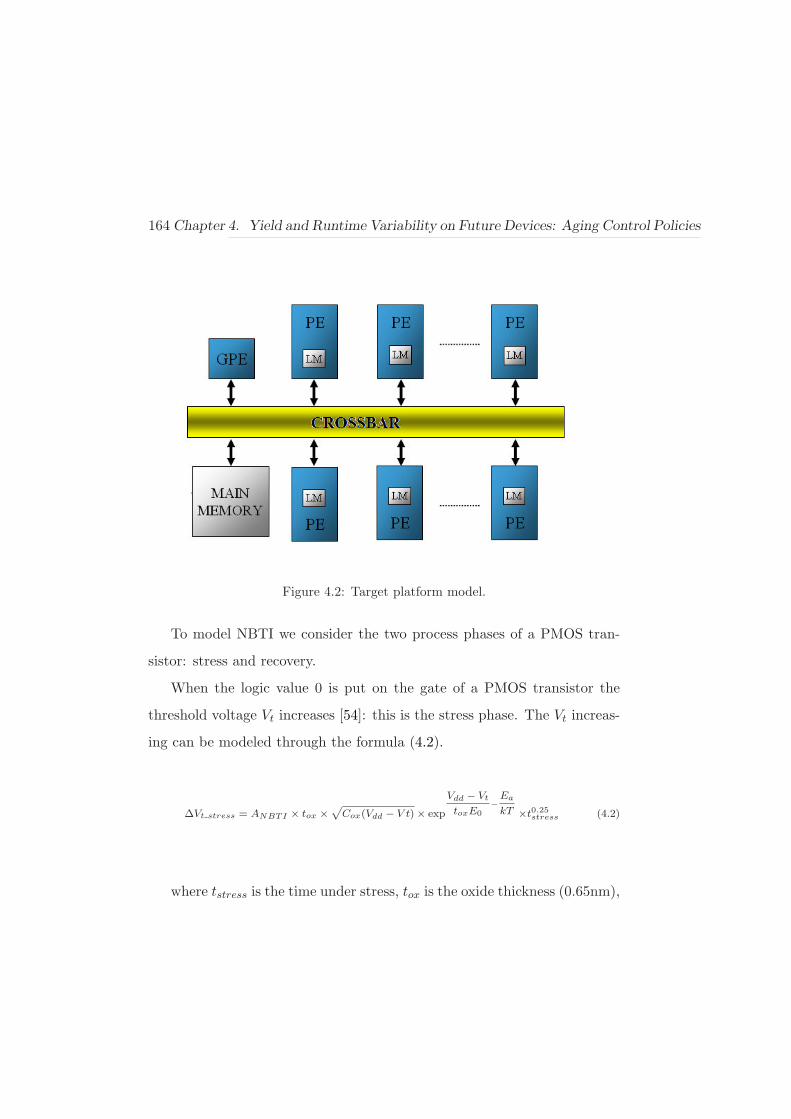
164 Chapter 4. Yield and Runtime Variability on Future Devices: Aging Control Policies
Figure 4.2: Target platform model.
To model NBTI we consider the two process phases of a PMOS tran-
sistor: stress and recovery.
When the logic value 0 is put on the gate of a PMOS transistor the
threshold voltage Vt increases [54]: this is the stress phase. The Vt increas-
ing can be modeled through the formula (4.2).
∆Vt stress = ANBTI × tox ×√
Cox(Vdd − V t)× exp
Vdd − Vt
toxE0
−
Ea
kT ×t0.25stress (4.2)
where tstress is the time under stress, tox is the oxide thickness (0.65nm),

4.4. NBTI-aware Platform Model 165
and Cox is the gate capacitance per unit area (4.6×10⁻²⁰F/nm2). E0, Ea,
and k are constants equal to 0.2V/nm, 0.13 eV , and 8.6174× 10− 5eV/K,
respectively. ANBTI is a constant that depends on the aging rate.
When a logic value 1 is put on the PMOS transistor, it turns off and
the recovery phase starts. In [98] authors model the final increasing of Vt
after both the phases of stress and recovery. The formula (4.3) describes
the final increasing.
∆Vt = ∆Vt stress × (1−√
η × trec/(tstress + trec) (4.3)
where trec is the time under recovery and η is a constant equal to 0.35.
To assess the impact of NBTI on the running software and enable the
study of system level software policies we integrated the NBTI model in
the target platform simulator. We created a plug-in using the xSTream
simulator API functions to have access to the simulator structures and
functionalities, such as to be able to scale the clock frequency from the
software program.
The plug-in is seen by the application as a device composed by a bank
of memory-mapped registers. It is possible to instanciate a device for each
xPE. The registers provide information about the threshold voltage Vt and
the clock frequency Fck of its own connected core.
The device must be configured setting the parameters of the model

166 Chapter 4. Yield and Runtime Variability on Future Devices: Aging Control Policies
shown above. The device uses simulator information to know the spent
cycles of the core in the different states (i.e. activity, idle, stall) so that it
can calculate through the clock frequency the stress time (activity) and the
recovery time (idle + stall) of the core.
When the user wants to know the current aging status, he sends a
request to the device through a dedicated pin, then the device writes the
current value of Vt onto the registers.
4.4.2 Task Migration Support
We implemented in the platform the software support to manage the mi-
gration of tasks among cores. As described in Section 4.4, the multicore
simulator consists of one ST231 processor and an array of xPE processors.
Henceforth we refer to the former as master and to the latter as slaves.
We name source core and destination core, respectively, the processor from
which the task is taken away and that to which the task is moved to. The
migration process is controlled by the master in a centralized manner. It
uses a shared memory zone to signal the two involved cores of the necessity
to perform the migration, by means of a flag. The migration mechanism is
realized using the checkpoint technique: the source core periodically checks
the status of the flag in shared memory and, if it is found enabled, it copies
its task context in a shared memory location, signals the destination core
raising an interrupt and puts itself in idle state. After that, the destination

4.4. NBTI-aware Platform Model 167
core reads and copies the task context from the shared memory to its local
memory, and starts executing the code. In this manner, the task is resumed
from the same point where it was interrupted in the source cpu. It must
be noted that this mechanism functions because we use the task replication
strategy (we used that in another work, see Section 2.3.2 for further de-
tails): when the master puts a new task in the system, every cpu copies the
task’s code in its local memory, but only one core executes it (that selected
by the master). Since every CPU has a copy of the original task, the task
context is enough to resume it. All above described is the case where one
task is moved from a core to an empty one (that is, it does not have any
task to run). If the destination is not empty, the tasks are swapped. The
swap, basically, is implemented performing two contemporary migrations.
Some considerations about the overhead caused by the migration infras-
tructure must be made. Thanks to the task replication mechanism, every
migration involves the transfer of just the task context, consequently there
is a very little amount of data to copy. Our experiments show that the
overhead is negligible. However there is a price to pay: task replication
wastes more memory space (see Section 2.3.2 for a complete evaluation of
this strategy).

168 Chapter 4. Yield and Runtime Variability on Future Devices: Aging Control Policies
4.5 Aging-aware Run-time Task Hopping
Our proposed aging policy exploits two distinct mechanisms: aging recovery
and task hopping. Here we explain them separately, mainly drawing the
attention to the underlying algorithms.
4.5.1 Aging Recovering Algorithm
This mechanism takes in charge the burden of assuring that the system will
not break down before the minimum wanted lifetime. Basically it reaches
the goal imposing recovery periods on the cpu that is becoming too old
(we are going to explain how we quantify that). It exploits the formulas
explained in Section 4.4.1: using as inputs the minimum desired lifetime,
the maximum frequency of the core and the threshold frequency (that is,
the frequency below which the cpu is considered dead), it extracts the
right trec/tstress ratio that guarantees the desired lifetime. The algorithm
periodically monitors the current ratio on each core, and if it finds that it
is lower than wanted, it forces the cpu to recover till the ratio is correct
again. It must be noted that what really matters to reach a certain lifetime
(for a certain formulas input set) is only the total recovery time over the
total stress time ratio, however they are distributed during the cpu life.
This mechanism imposes a penalty on the cpu, lowering its overall work.
We can think of that in term of CPU effective frequency: forcing a core to
go in idle for recovering purpose means that it is available, in average, for
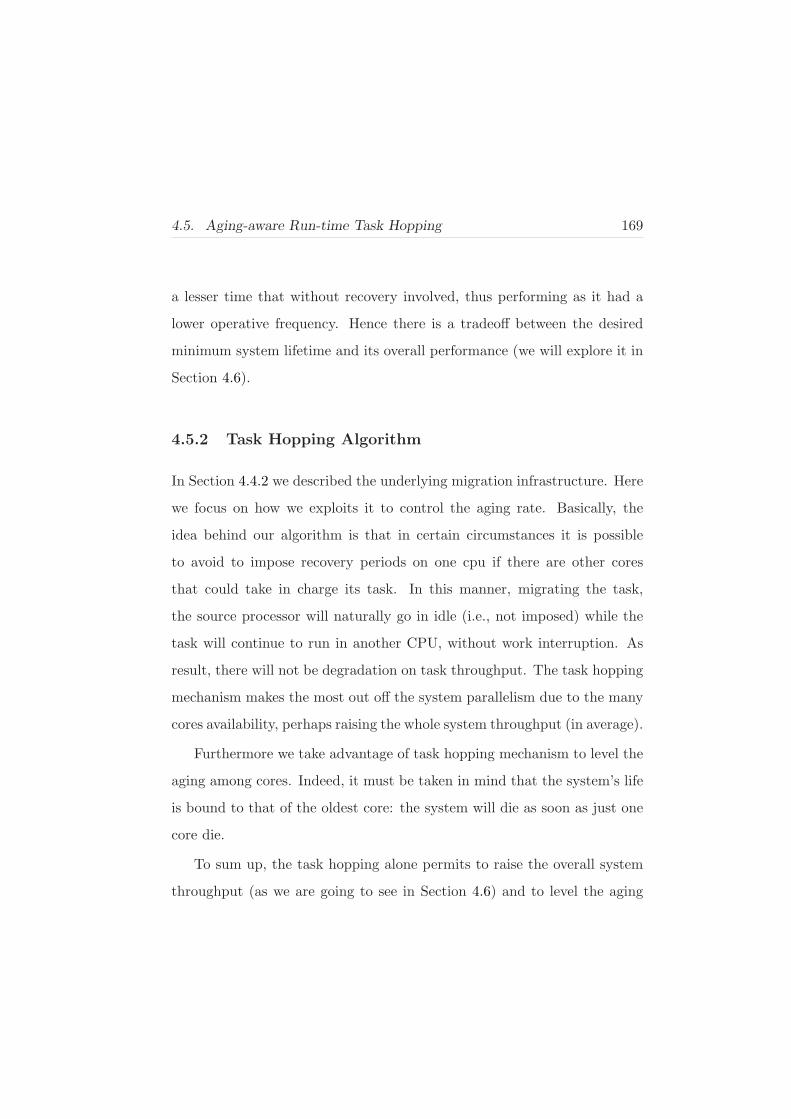
4.5. Aging-aware Run-time Task Hopping 169
a lesser time that without recovery involved, thus performing as it had a
lower operative frequency. Hence there is a tradeoff between the desired
minimum system lifetime and its overall performance (we will explore it in
Section 4.6).
4.5.2 Task Hopping Algorithm
In Section 4.4.2 we described the underlying migration infrastructure. Here
we focus on how we exploits it to control the aging rate. Basically, the
idea behind our algorithm is that in certain circumstances it is possible
to avoid to impose recovery periods on one cpu if there are other cores
that could take in charge its task. In this manner, migrating the task,
the source processor will naturally go in idle (i.e., not imposed) while the
task will continue to run in another CPU, without work interruption. As
result, there will not be degradation on task throughput. The task hopping
mechanism makes the most out off the system parallelism due to the many
cores availability, perhaps raising the whole system throughput (in average).
Furthermore we take advantage of task hopping mechanism to level the
aging among cores. Indeed, it must be taken in mind that the system’s life
is bound to that of the oldest core: the system will die as soon as just one
core die.
To sum up, the task hopping alone permits to raise the overall system
throughput (as we are going to see in Section 4.6) and to level the aging

170 Chapter 4. Yield and Runtime Variability on Future Devices: Aging Control Policies
among all cores.
4.6 Experimental results
In this section we show how our policy is able to control the aging rate
and we explore its impact on the system’s performance. In order to as-
sess the aging policy, we implemented a multitask synthetic application
that models different idle patterns among tasks. We did that in order to
model real life scenarios of applications characterized by different workload
patterns among tasks. This benchmark application consists of three inde-
pendent synthetic tasks, each one executing some dummy work, quantified
by increasing a counter. The workload of each task is modeled in three
phases (namely a cycle) that repeat to infinity. In the first phase, the task
is always-on, that is, the CPU that executes it work at 100%. This phase
lasts for a fixed period, always the same. In the second phase, only one
task is fully working (that is, at 100%), whilst the others are in idle. This
phase lasts for a variable period (we vary this period in such a manner
to model different overall application’s workload pattern). Finally, in the
third phase, the task is in idle, for a fixed period. Thus, all phases but the
second, have a fixed length. Figure 4.3 visually summarizes all that above.
We performed several experiments varying the second phase’s length,
aiming at modeling applications with different workload patterns among
tasks.

4.6. Experimental results 171
Phase 1 Phase 2 Phase 3
Task 1
Task 2
Task 3
100% working
100% working
100% working
100% working
idle
idle
idle
idle
idle
fixed length variable length fixed length
1 cycle
Figure 4.3: Task modeling
We tested such application in a multiprocessor testbed (described in
Section 4.4), using both three and four CPUs, to better stress the aging
policy (note that, in any case, the test application is always composed by
three tasks).
4.6.1 Aging Rate Tuning
Here we experimentally show how our proposed aging policy functions. It
takes as input the wanted system lifetime, defined as the time when at least
one processor will die. The policy, following this constrain, imposes a lower
bound to the system lifetime, assuring that the system will never break
down early.

172 Chapter 4. Yield and Runtime Variability on Future Devices: Aging Control Policies
As described in Section 4.3, aging influences the maximum frequency of
the CPU, decreasing it with a certain rate, depending on the stress it was
submitted to. The core will break down as soon as its frequency goes under
a certain threshold. The aging policy we proposed controls the maximum
frequency’s trend, guaranteeing that it will not reach that limit before the
imposed lifetime. All above is showed in Figure 4.4, that sketches the
maximum frequency of one CPU over the time, comparing the case without
policy versus the case with the policy, for different imposed lifetimes. The
time is normalized with respect to the lifetime of the case without policy,
picked up as a reference point. The above data are obtained using three
cores and three tasks, without task hopping, at a given task cycle pattern
(that is, at a given three phase pattern), to show the behaviour of the
recovery algorithm alone. These experiments demonstrate that using the
policy, the CPU respects the wanted lifetime and explain how it influences
the trend (over the time) of the maximum frequency.
The main advantage of raising the system lifetime is that it can produce
a greater overall work, as pointed out by Figure 4.5. It has been realized
using four CPUs, three tasks, at a given task cycle pattern, for three sce-
narios: without policy, with aging policy but without hopping feature and
with aging policy fully operative (i.e., with hopping enabled). As in the
previous image, the time is normalized with respect to the lifetime of the
case without policy. Even the overall work is normalized with respect to
the total work of the no policy case. Thus, there is a sensible increase of

4.6. Experimental results 173
400
450
500
550
600
0 1 2 3 4 5 6 7 8 9 10 11 12
Normalized Time
Fre
qu
en
cy (
MH
z)
NO-POLICY
POLICY 1.8x
POLICY 3.6x
POLICY 5.4x
POLICY 10.9x
Figure 4.4: Maximum CPU frequency over the time, for different imposed lifetimes
system work. Note that when the hopping is enabled, there is a greater
raise of the work, because it exploits the fourth CPU.
0
1
2
3
4
5
6
7
8
3 4 5 6 7 8 9 10 11
Normalized Lifetime
No
rmali
zed
to
tal w
ork
hopping
no hopping
Figure 4.5: Total system work varying the imposed lifetime
This increase of total work is due to the fact that if we leave the system

174 Chapter 4. Yield and Runtime Variability on Future Devices: Aging Control Policies
without rate control, the amount of work is limited by the premature death
of the system. The imposed recovery periods avoid that early end, but a
price. In fact, there is a penalty caused by the policy: the CPU effective
frequency (this concept has been defined in Section 4.5.1) is lesser than the
real one, thus its amount of work per unit of time (namely throughput)
is lower. This penalty is shown in Figure 4.6: it depicts the average sys-
tem throughput for different lifetime values. As before, both throughput
and lifetimes are normalized with respect to the no policy case. The data
are related to the same experiment of Figure 4.5, so the setup is as de-
scribed there. It shows the tradeoff between wanted minimum lifetime and
performance: more we want the system to last, more we have to penalize
it, forcing longer recovery periods. Equivalently, we can state: more we
want the system to last, more we have to decrease its effective frequency,
thus causing less work per unit of time (i.e., less throughput). It must be
noted that the big difference between hopping and no-hopping cases (in
the showed figure) is because the former exploits the fourth cpu, that is not
used in the latter (remember that we use three tasks). We will explore in
the next section (Section 4.6.2) the real advantage of the hopping approach
over the no-hopping one, even with only three CPUs (we will see that the
hopping itself increases the performance).

4.6. Experimental results 175
0
0.2
0.4
0.6
0.8
1
3 4 5 6 7 8 9 10 11
Normalized Lifetime
No
rmalized
Th
rou
gh
pu
t
hopping
no hopping
Figure 4.6: Policy’s penalty assessment at different imposed lifetimes
4.6.2 Performance Assessment
In the previous section, we showed the basic functioning of the aging policy,
using always the same task configuration. In this part of the experimental
section instead we show the improvement on the performance allowed by
the proposed policy in various configurations of the task set (that is, varying
the second phase length of the tasks), and at a given imposed lifetime. In
this manner, we aim at modeling several real life scenarios, characterized
by different workload patterns among tasks. Furthermore, we performed
experiments using both three and four CPUs, but we consider always an
application composed by three tasks.
In Figure 4.7 we compare our policy in two configurations: with and
without task hopping. The results represent the gain, in percentage, of

176 Chapter 4. Yield and Runtime Variability on Future Devices: Aging Control Policies
the hopping approach with respect to the no hopping one, varying the
percentage of idleness among tasks (we plotted the standard deviation of
the percentage of idleness). In the case of four CPUs there is a great gain,
mainly due to the exploitation of the additional CPU, because without task
hopping only three CPUs are used (keep in mind that the application is
composed by three tasks, always), thus the results are quite predictable. It
is worth noting that the gain is almost constant. The case with three CPUs
instead reveals that the task hopping raises the amount of total work even
with a number of CPUs equal to the number of tasks. This improvement
is due to the better exploitation of the platform parallelism allowed by
the task migration (it exploits the idleness in other CPUs). It also shows
that the gain depends on the difference of idleness among CPUs. There is
something else to underline: as noted above, in all these experiments the
system lifetime is the same, hence the total work in all cases is obtained in
the same time, so the results in Figure 4.7 can be considered as a throughput
gain (in %) as well. That leads to the consideration that, in the case of three
CPUs, the hopping mechanism increases the throughput of the system, thus
being more efficient.
4.7 Conclusions
Experiments demonstrate that our policy, exploiting both aging rate har-
nessing mechanisms and task migration, is able to control the aging phe-
4.7. Conclusions 177
Hopping gain with respect to no-hopping
0
5
10
15
20
25
30
35
40
0 5 10 15 20 25
Standard deviation of %idle among CPUs
To
tal w
ork
Gain
(%
)
3 CPUs
4 CPUs
Figure 4.7: Total work gain of the hopping mechanism over the no-hopping one,
increasing the idleness among tasks
nomena bounding the system’s lifetime at desired values while minimizing
the overhead penalty. My research in this field is currently in progress and
new experiments are about to be performed. In particular, we are going to
assess our policy with respect to an optimal solution.

178 Chapter 4. Yield and Runtime Variability on Future Devices: Aging Control Policies

Chapter 5
Scheduling-Integrated
Policies for Soft-Realtime
Applications
During my PhD researches I mainly worked about developing fully-integrated
solutions for power/energy and variability/aging management. In the ef-
fort to integrate the policies at system level, it soon turned out the need
of acting at scheduling level, in such a manner to have the maximum con-
trol over the system. Then I started approaching scheduling issues in both
single and multiprocessor systems, particularly targeting soft realtime ap-
plications, that are the common kind of applications I dealt with in most of
my works. Henceforth I researched a new scheduling algorithm specifically
180 Chapter 5. Scheduling-Integrated Policies for Soft-Realtime Applications
thought to be fully integrated with power/thermal management policies. I
realized it in the Linux operating system, given that is becoming ever more
diffused even in embedded systems. Nevertheless, the scheduling itself could
be easily developed in platforms without operating systems.
This work, still under further extensions, aims at being the last piece
of a set of tools for reaching a fully-integrated software solution for next
generation devices.
5.1 Introduction
Multimedia applications are increasingly complex and demanding in terms
of both computational power and time constraints. A good example is
given by the increasing resolution and frame rate requirements of video
streaming applications. When these applications run on top of a general
purpose operating system their requirements become very challenging. In-
deed, these OSes are currently used in system with demanding networking
capabilities, where multiple network flows must be managed. This is true
not only for desktop PCs, but also in embedded networking systems such
as media gateways, where general purpose OSes are of widespread use for
cost and flexibility reasons. Besides typical network processing, these sys-
tems must perform various general purpose processing at line rate such as
video decoding, video transcoding, image processing and encryption. Now,
in general purpose OSes, the scheduler is not specifically designed for han-
5.1. Introduction 181
dling real-time requirements even if a support for real-time processes does
exist in well known general purpose OSes such as Linux or Windows. How-
ever, this support simply gives, to a process defined as “real-time”, a static
priority higher than any other “conventional process”.
The main issue is that current generation multimedia applications are
composed by a cascade of multiple dependent tasks communicating by
means of message queues. For instance, a H.264 decoder is composed by
several steps including motion compensation, entropy decoding, dequanti-
zation, inverse Discrete Cosine Transform (DCT). Furthermore, multimedia
frameworks such as GStreamer create complex multimedia applications by
chaining several stages [41]. In both cases, the frame rate (i.e. QoS) re-
quirements are backward propagated from the last stage to the previous
ones. A general purpose scheduler, such as the Linux one, is not aware of
task dependencies and timing constraints, but only looks at how much a
task is demanding in terms of CPU utilization.
The “conventional process” scheduler is designed to promote, by giv-
ing them a high dynamic priority, the so called I/O bounded applications.
These are characterized by small (compared to the timeslice) CPU bursts
interleaved to large I/O access periods. CPU bounded ones, instead, are
characterized by much larger CPU bursts, and thus are given a smaller dy-
namic priority. This is because I/O applications are supposed to interact
with the user and so the OS attempts to reduce their latency. On the other
side, the real-time process scheduler in Linux implements either a FIFO

182 Chapter 5. Scheduling-Integrated Policies for Soft-Realtime Applications
or a Round-Robin policy. Both of them, as we are going to show later
on, do not take into account actual requirements of tasks, leading to QoS
degradation especially in high CPU utilization conditions.
An additional limitation of general purpose OSes arises in presence of
multiple real-time applications running simultaneously, as in the context
of media gateways, where several streams need to be decoded at the same
time to feed multiple network connections. Here the computational power
must be allocated to multiple decoding applications having heterogeneous
QoS requirements, such that all they perceive a degradation proportional to
their QoS requirements. This can be hardly achieved using general purpose
OSes that lack the concept of fairness related to the QoS.
Putting it all together, general purpose schedulers are not longer suit-
able to modern multimedia applications ( [69], [31]). Nevertheless, they
are still common in Windows family, Linux, and all other variants of Unix
such as Solaris, AIX and BSD (see [32] for more details).
An alternative solution would be to adopt real-time schedulers devel-
oped for real-time embedded systems, that are suitable to situations where
the deadlines must be strictly respected (e.g., life-safety critical applica-
tions). The counterpart is that they are hard to manage and they require
to explicitly provide the scheduler with time constraints information of ap-
plications (i.e. deadlines) that must be hence modified accordingly.
In this work I propose a variant of the Linux scheduler, called queue-
based scheduler (QBS) that deals with soft real-time streaming applications

5.1. Introduction 183
composed by multiple pipelined stages. QBS is aware of QoS requirements
of multitask applications similarly to real-time schedulers, but does not re-
quire application modifications, as general purpose ones. To achieve this
objective, it monitors the intertask communication and requires the instru-
mentation of the communication and synchronization library.
QBS assumes that applications are composed by multiple pipelined
stages that communicate by means of queues of messages. Such applica-
tions follow a data-flow paradigm, where tasks continuously process frames
arriving in their input queue and produce frames on their output queue for
the next processing stage. Figure 5.1 shows an example of such paradigm
(H.263 decoder). Most modern multimedia applications are realized in such
a manner (e.g., audio/video decoders).
Input TaskOutputTask
H.263Video
Streaming
Task 1
Task 2
Task n
... Application
output queue
Task
output queues
Consumerread
Task
input queues
Figure 5.1: Pipelined multi-stage application scheme (H.263 Decoder)
In this kind of applications the application output queue is read at fixed
time intervals and if it is found empty a deadline miss occurs. The main
idea behind QBS is to monitor the queue occupancy level of all queues

184 Chapter 5. Scheduling-Integrated Policies for Soft-Realtime Applications
in the system and to take scheduling decisions based on this information.
Basically, QBS seeks the emptiest queue in the system and schedules the
process or task writing into it. Thus QBS can quickly react to situations
that may lead to deadline misses, exploiting the feedback from the queues.
In the considered application model, QoS is preserved as long as there
are data items available in the application output queue (that is, the last
queue of application) when they are needed by the final consumer stage.
This leads to two very important considerations. First, the application
output queue can be even empty in some periods of time without necessar-
ily having misses. Second, intermediate stages have less stringent timing
requirements in general.
The queue feedback approach ensures a more effective CPU time alloca-
tion to each task, based on its real and actual QoS requirements. In prac-
tice, the level of occupancy of the output queue of a task is used as a measure
of its CPU utilization needs. A deep explanation of that, together with a
detailed description of the proposed algorithm, is provided in Section 5.3.
To test its effectiveness, we implemented the scheduler inside Linux OS and
we instrumented the standard System V message queue library to support
monitoring features. Thanks to this implementation, we performed various
sets of experiments with a single and multiple video decoding applications.
We compared the deadline miss rate of QBS w.r.t. default real-time and
conventional process scheduler in case of single and multiple decoding appli-
cations having heterogeneous QoS requirements. Results demonstrate that

5.2. Related Work 185
QBS improves the deadline miss rate in high CPU utilization conditions
and provides better CPU resource allocation, that is proportional to frame
rate requirements.
The rest of the chapter is organized as follows: Section 5.2 describes
related work in the area of scheduling for real-time and multimedia appli-
cations. Section 5.3 full details the QBS algorithm, Section 5.4 explains
why we chose Linux as testbed platform, Section 5.5 describes our imple-
mentation while Section 5.6 shows the experimental results. Section 5.7
gives the conclusions.
5.2 Related Work
In literature many approaches have been proposed to manage soft real-time
applications in commodity OSes. [30] performs a deep evaluation of how
clock interrupt frequency influences the response time of multimedia appli-
cations. Their study aims at helping tuning existing schedulers. Similarly,
other techniques as soft timers [4], firm timers [39] and one-shot timers
have been proposed to significantly enhance response time. However, none
of them propose a new scheduler algorithm but rather latency reduction
techniques.
On the other side, many real time schedulers have been proposed.
SMART [70] is a scheduler for multimedia and real time applications im-
plemented in UNIX-like OSes. It schedules real time tasks even trying to

186 Chapter 5. Scheduling-Integrated Policies for Soft-Realtime Applications
avoid the starvation of conventional processes, but it requires deep modifi-
cations of existing applications. In fact, applications have to communicate
their deadlines to the scheduler which can also return feedbacks to enable
some proactive countermeasure (e.g., re-modulate their workload in order
to meet the deadline). On Linux, some examples are Linux/RK [72], RTE-
Linux [101], Linux-SRT [21] and RTLinux [8]. These all have the same
general drawbacks of real-time schedulers (i.e. programmers must use a
dedicated interface to exploit these services). Other approaches explicitly
require user intervention to specify the needs (in terms of priority) of the
processes or of a class of processes (e.g., multimedia applications) [21] [78].
The algorithm proposed in this research (QBS) provides QoS sensitive
scheduling without requiring explicit user awareness and or modification of
existing applications, given that they follow the message queue paradigm.
As mentioned in the introduction, this model adheres with the one of mod-
ern multimedia applications and frameworks.
5.3 Queue-based Scheduling Algorithm
The idea behind the proposed algorithm is to exploit the queue level as
indication of task requirements and consequently to grant CPU time pro-
portionally to that. For example, let us consider a simple case of two appli-
cations, A and B, with a CPU need of 65% and 55% respectively. Running
them in a standard operating system, without any knowledge of applica-
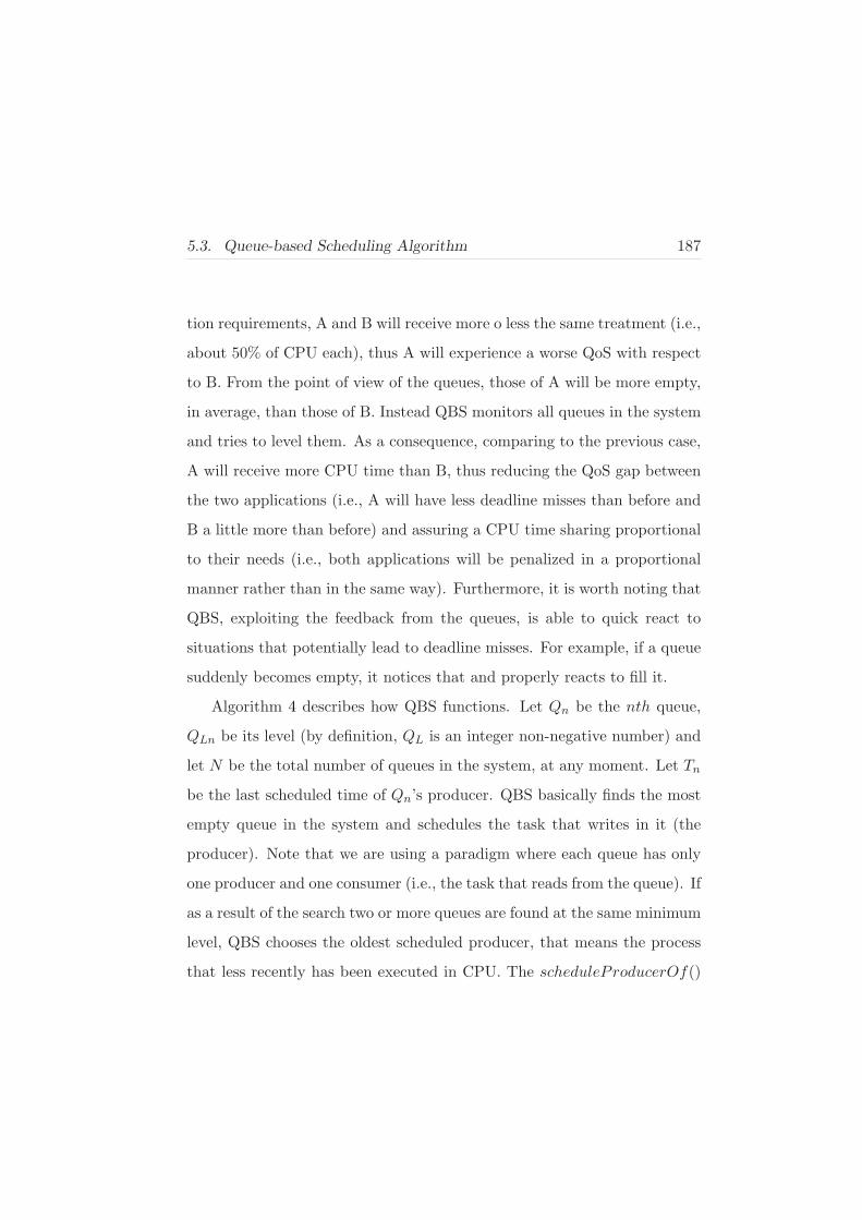
5.3. Queue-based Scheduling Algorithm 187
tion requirements, A and B will receive more o less the same treatment (i.e.,
about 50% of CPU each), thus A will experience a worse QoS with respect
to B. From the point of view of the queues, those of A will be more empty,
in average, than those of B. Instead QBS monitors all queues in the system
and tries to level them. As a consequence, comparing to the previous case,
A will receive more CPU time than B, thus reducing the QoS gap between
the two applications (i.e., A will have less deadline misses than before and
B a little more than before) and assuring a CPU time sharing proportional
to their needs (i.e., both applications will be penalized in a proportional
manner rather than in the same way). Furthermore, it is worth noting that
QBS, exploiting the feedback from the queues, is able to quick react to
situations that potentially lead to deadline misses. For example, if a queue
suddenly becomes empty, it notices that and properly reacts to fill it.
Algorithm 4 describes how QBS functions. Let Qn be the nth queue,
QLn be its level (by definition, QL is an integer non-negative number) and
let N be the total number of queues in the system, at any moment. Let Tn
be the last scheduled time of Qn’s producer. QBS basically finds the most
empty queue in the system and schedules the task that writes in it (the
producer). Note that we are using a paradigm where each queue has only
one producer and one consumer (i.e., the task that reads from the queue). If
as a result of the search two or more queues are found at the same minimum
level, QBS chooses the oldest scheduled producer, that means the process
that less recently has been executed in CPU. The scheduleProducerOf()

188 Chapter 5. Scheduling-Integrated Policies for Soft-Realtime Applications
function schedules the producer of the queue passed to it as argument.
Algorithm 4 Queue-based scheduler algorithmEvery decision instant do:
1: Qmin = Q1
2: Tmin = T1
3: for n = 1 to N do
4: if (QLn < QLmin) OR (QLn = QLmin AND Tn < Tmin) then
5: Qmin = Qn
6: Tmin = Tn
7: end if
8: end for
9: scheduleProducerOf(Qmin)
The last point to analyse is how frequently QBS should be executed.
There is clearly a trade-off here, indeed: choosing a high frequency achieves
a better leveling of the queues, but, on the other hand, it increases the
number of context switches, thus causing a higher overhead. Thus, we chose
to maintain the concept of Linux timeslice: every process can consecutively
use the CPU till a maximum amount of time (i.e., the timeslice), at the
end of which the scheduler is called and the current process (most of the
times) is preempted and another one is scheduled.

5.4. Testbed System Description 189
5.3.1 QBS Complexity
The algorithm’s complexity is related to the necessity to scan all the queues
in the system to find the most empty one. Thus QBS would have a linear
complexity, that is O(n) (where n is the total number of active queues in the
system). Given that the scheduler is called very frequently, it is mandatory
to reduce its complexity as much as possible. We then reduced it to O(1),
that means it no longer depends on the number of the queues. This result
has been obtained using a special data structure to keep trace of all the
queues and considering that, at any moment in time, the only ones that
could change are those read and written by the task currently in execution.
So, when the scheduler is invoked, it quickly updates the information about
the only queues that could have been changed. Hence, the time taken for
this operation is constant (O(1)). The details of how we implemented it
are described in Section 5.5.1
5.4 Testbed System Description
We chose to implement QBS in Linux 2.6, thanks to its open source nature
and widespread diffusion. It is used in desktop PCs, many server systems
(e.g., web, mail, dns, routers, etc.) and, recently, in mobile platforms
too. The most important example of that is probably Android [40], the
Google OS for smartphones, based on Linux and widely thought to reach a
leading position in the sector very soon. QBS aims at be adopted in above

190 Chapter 5. Scheduling-Integrated Policies for Soft-Realtime Applications
systems and even in small/medium multimedia servers (e.g., audio/video on
demand, voip, etc.), where expensive high specific solutions (e.g., real time
OSes) are not affordable and commodity operating systems are the usual
choice. Thus, in all these systems the standard Linux scheduler is adopted.
We decided for this reason to compare QBS versus Linux standard policies.
The following section (5.4.1) details these policies.
5.4.1 Linux Standard Policies
Linux standard distributions come with three policies (some slight varia-
tions are possible depending on kernel versions, but they are basically the
same): SCHED NORMAL, SCHED RR and SCHED FIFO. The first one
is the default policy for all tasks. It is a relatively complex algorithm that
deals with conventional processes (i.e., not real time processes). It con-
tinuously attempts to identify interactive tasks from CPU intensive ones,
using the common mechanism (common to many OSes) described early:
processes that spend most of their time waiting for I/O operations are sup-
posed to be interactive, while those that heavily exploit the CPU fall in the
second category. Then the scheduler grants more priority to the interactive
ones, in order to reduce their latency. Unfortunately nowadays interactive
multimedia applications are CPU greedy too, thus they are penalized by
this mechanism. For this reason this policy is not adequate for managing
interactive applications (we are showing that in Section 5.6.2).

5.5. Implementation Details 191
SCHED RR and SCHED FIFO are both real time algorithms: basically
the former (round robin policy) equally shares the CPU times among tasks,
while the latter (fifo policy) grants all CPU time to the first arrived process
as far as it uses it, after that it schedules the next task in the FIFO queue.
Thus the last one, given its fifo behaviour, it is not adequate for multimedia
applications (it does not treat all processes fairly). Instead round robin
(RR) performs quite well and consequently is the main algorithm we are
going to confront against (Section 5.6.2). It must be noted that Linux real
time policies are intended to manage soft real time processes. To specify a
task as a real time one, the programmer needs only to state that using a
system call. No any other modification is needed. Alternatively, the user
can set it using the chrt linux command, without any modification to the
application code.
5.5 Implementation Details
This section describes how we implemented QBS in a standard Linux kernel.
In particular, all details are referred to kernel 2.6.20.16.
5.5.1 Scheduler
This section gives some details on how we modified the Linux scheduler in
such a way to include our new algorithm. The Linux scheduler picks up the
next task to be executed from the top of a specialized task queue. Thus,

192 Chapter 5. Scheduling-Integrated Policies for Soft-Realtime Applications
we decided to call our routine (i.e., the code that implements our algorithm
and chooses the next task to be scheduled) just right before this choice, in
such a manner to put the process selected by QBS on top of that queue.
In this way, the scheduler will find in it the task we decided.
In Section 5.3 we described the algorithm and in Section 5.3.1 we stated
that its complexity is O(1). We realized all above using the structure
showed in Figure 5.2. It is an array of simply linked lists, where MAX
represents the maximum possible number of elements in a queue (i.e., a
System V message queue). Each element of the lists is a queue identifier,
that means it points to an allocated queue. The key point here is that,
at any moment in time, each element in the nth list (i.e., that at position
n in the array) points to a queue of n element (a that time). Thus the
algorithm described in Section 5.3 is implemented in this way: it scans the
array starting from 0 and selects the first element found. Hence, it points
to the most empty queue in the system, as requested by the algorithm.
The queue identifier is composed by three fields: (i) lid is a pointer to one
queue; (ii) timestamp represents the last scheduled time of the producer
of that queue; (iii) next is a pointer to the next element in the linked list.
It must be noted that in each list, all elements are ordered in a temporal
way using the timestamp, from left to right, where on the left there is the
oldest one. Hence this assures that the first element found during the scan
of the array represents both the producer of the most empty queue in the
system and, among all queues at the same level, the oldest scheduled one.

5.6. Experiments 193
Moreover this structure assures that the time spent for selecting a task is
constant (O(1)), because it not depends on the number of the tasks.
This structure is updated every time the scheduler is called: it checks
only the queues modified by the last executed task and, if needed, moves
the corresponding identifiers in the correct array position.
0
1
MAX
NULL
NULL
NULL
LID TIMESTAMP NEXT
QUEUE IDENTIFIER
Figure 5.2: Array of simply linked lists of queue identifiers
5.6 Experiments
This section describes the experimental setup and the tests we performed
to evaluate QBS.
5.6.1 Experimental Setup
We setup a dedicated machine for all the experiments, equipped with a CPU
Athlon XP 1100 GHz and with 512 MB of RAM. For the reasons explained
in Section 5.4.1, we compare primarily against the Linux standard round

194 Chapter 5. Scheduling-Integrated Policies for Soft-Realtime Applications
robin policy (SCHED RR). Nevertheless, we performed some comparisons
versus SCHED NORMAL (conventional) algorithm too. We set up sev-
eral experiments using two basic applications, both following the message
queue paradigm described early in Section 5.1. The first one, depicted in
Figure 5.3, is composed by synthetic tasks (i.e., they perform some useless
work). Instead the second one is a real H.263 decoder, already showed in
Figure 5.1. The movie to be decoded is full loaded in RAM before the start
of experiments, in such a manner to avoid possible bottlenecks during its
read from the hard disk. The memory is then locked to prevent swapping.
All these operations are done by the Input Task, that then decomposes each
frame of the video in n parts and puts them in the next proper queue. Each
following task (Task 1 to n) elaborates the nth part of the frame. In the
end, the Output Task reassembles the decoded frame, does some elaboration
and puts it in the application output queue.
It must be noted that in both applications we use the System V message
queue library. All operations on queues (read and write) are blocking, that
means if a process attempts to read in a empty queue or to write in a full
one, it is suspended and automatically woken up as soon as this situation
changes.
As metric for comparing QBS versus Linux standard algorithms we
chose the QoS, obtained by counting the number of deadline misses. These
events happen every time no data are found in the application output queue,
at the right moment. Indeed the output queue of each application instance

5.6. Experiments 195
Task 1
Task 2
Task 3
Task 4
final queue
Figure 5.3: Synthetic task application
is read at a fixed frequency, depending on the wanted frame rate. From
a practical point of view, we implemented a single real time task with a
greater real time priority than all others, that periodically reads the output
queue of all applications. The higher priority is needed in order to guarantee
the strict periodicity of its reads.
We wanted to compare the algorithms in a real-world situation, hence
we decided to implement a media server, using the two decoders described
before as basis. Thus, we set up many experiments with several instances
of such applications running in parallel, and varying their parameters, as
task workload, frame rate, and so on.
5.6.2 Experimental Results
First off, we executed some experiments with the synthetic application,
comparing against both SCHED RR and SCHED NORMAL. Figure 5.4

196 Chapter 5. Scheduling-Integrated Policies for Soft-Realtime Applications
shows the deadline misses (in percentage with respect to the total number
of reads at the application output queue) versus the frame rate, running
two application instances in parallel. The miss rate plotted is the average
between the two values (note that each application has its own deadline
misses). In these experiments QBS performs better than the others, having
always less misses. Furthermore it sustains an higher frame rate without
having QoS worsening (namely, 26.4 fps versus 25.8 fps for SCHED RR
and 22.9 fps for SCHED NORMAL). Here we want to underline one aspect
that reveals how SCHED NORMAL is not adequate for comparing versus
QBS: numerical results (not reported) show that there is a great gap of
performance between the two application instances. For example, it can
happen that one application has zero misses for a very long time while the
other has 15% of it. This is because SCHED NORMAL is not thought to
deal with soft real time processes and furthermore it continuously tries to
prioritize interactive tasks (this mechanism is described in Section 5.4.1).
This is the reason why we do not compare against it anymore.
Using a debug monitoring infrastructure, we carefully analyzed the be-
haviour of all the queues over the time, observing that QBS is able to level
them (in average) while RR shows great differences. It is possible to ob-
serve this behaviour in Figure 5.5. For example (RR case), some queues
are totally full while others are completely empty. The main consideration
here is: if a queue is always almost empty (in average) and another is in
the opposite condition, probably the CPU time could be more fairly dis-

5.6. Experiments 197
Synthetic Tasks: 2 application instances
0.00%
1.00%
2.00%
3.00%
4.00%
5.00%
6.00%
7.00%
8.00%
22.5 23.0 23.5 24.0 24.5 25.0 25.5 26.0 26.5 27.0 27.5 28.0
Frame Rate (fps)
De
ad
lin
e M
iss
es
(%
)
QBS
Round Robin
Conventional
Figure 5.4: Synthetic tasks: deadline misses versus frame rate
tributed (i.e., more CPU time than needed is granted to the task which
output queue is fuller). Instead QBS shows the capacity to better level
all queues in the system, in average, suggesting a smarter CPU repartition
among tasks.
In the following examples we are going to stress more both algorithms,
using many instances of the H.263 decoder. We started using six parallel
instances and then up to eighteen (note: in this set of experiments all
instances are perfectly identical and the input file is the same). Figure 5.6
shows the deadline misses (in percentage) versus the frame rate for six
applications (note: the value is the average among all applications). It is
possible to see that QBS performs slightly better (similar results apply for
the other above mentioned cases, that is with more than six decoders).
However, the differences are really tiny. But, even if the total QoS

198 Chapter 5. Scheduling-Integrated Policies for Soft-Realtime Applications
QBS
0
2
4
6
8
10
12
0 5 10 15 20 25 30Time (sec)
Qu
eu
e L
evel Task 1
Task 2
Task 3
Task 4
RR
0
2
4
6
8
10
12
0 5 10 15 20 25 30Time (sec)
Qu
eu
e L
ev
el Task 1
Task 2
Task 3
Task 4
Figure 5.5: Queue levels over time
is a significant metric, is not the most important one. Indeed, a more
valued characteristic is its uniformity, both per and among applications.
That means that it is not desirable to have, for instance, a decoder that
performs very well while another is working very bad, but rather to have
all them with the same QoS level (ideally), at any time (to understand
that it must be kept in mind that in this set up all instances are perfectly
identical). The two plots in Figure 5.7 show the miss percentage over the
time for each application (eighteen decoders at the same fixed frame rate).
Even if it is not possible to distinguish every singular application, its aim is
to display how QBS is able to much better level the QoS among decoders.
Indeed the lines in the QBS plot appear closer each others. To numerically
quantify this behaviour, we calculated the standard deviation of deadline
misses among decoder instances, at fixed interval times. The results reveal
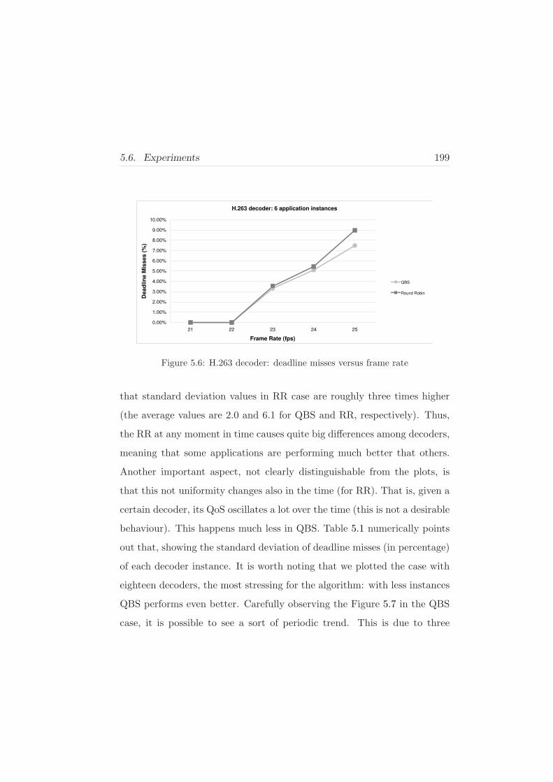
5.6. Experiments 199
H.263 decoder: 6 application instances
0.00%
1.00%
2.00%
3.00%
4.00%
5.00%
6.00%
7.00%
8.00%
9.00%
10.00%
21 22 23 24 25
Frame Rate (fps)
De
ad
lin
e M
iss
es
(%
)
QBS
Round Robin
Figure 5.6: H.263 decoder: deadline misses versus frame rate
that standard deviation values in RR case are roughly three times higher
(the average values are 2.0 and 6.1 for QBS and RR, respectively). Thus,
the RR at any moment in time causes quite big differences among decoders,
meaning that some applications are performing much better that others.
Another important aspect, not clearly distinguishable from the plots, is
that this not uniformity changes also in the time (for RR). That is, given a
certain decoder, its QoS oscillates a lot over the time (this is not a desirable
behaviour). This happens much less in QBS. Table 5.1 numerically points
out that, showing the standard deviation of deadline misses (in percentage)
of each decoder instance. It is worth noting that we plotted the case with
eighteen decoders, the most stressing for the algorithm: with less instances
QBS performs even better. Carefully observing the Figure 5.7 in the QBS
case, it is possible to see a sort of periodic trend. This is due to three
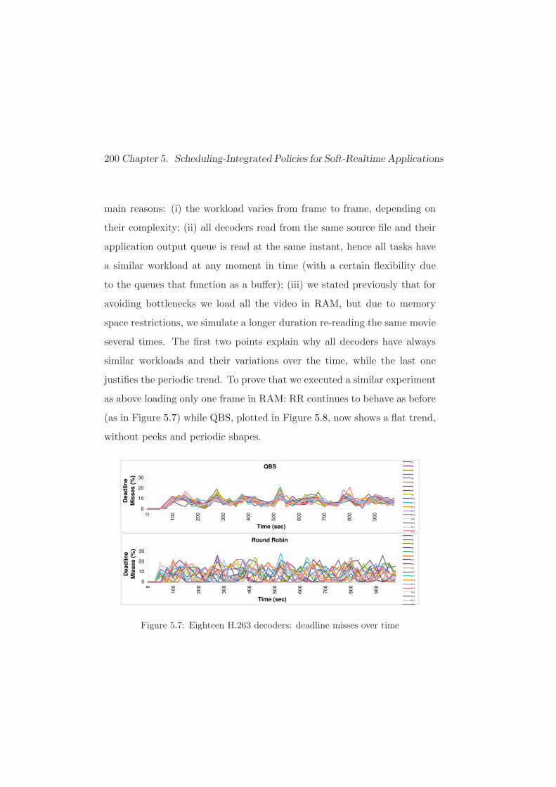
200 Chapter 5. Scheduling-Integrated Policies for Soft-Realtime Applications
main reasons: (i) the workload varies from frame to frame, depending on
their complexity; (ii) all decoders read from the same source file and their
application output queue is read at the same instant, hence all tasks have
a similar workload at any moment in time (with a certain flexibility due
to the queues that function as a buffer); (iii) we stated previously that for
avoiding bottlenecks we load all the video in RAM, but due to memory
space restrictions, we simulate a longer duration re-reading the same movie
several times. The first two points explain why all decoders have always
similar workloads and their variations over the time, while the last one
justifies the periodic trend. To prove that we executed a similar experiment
as above loading only one frame in RAM: RR continues to behave as before
(as in Figure 5.7) while QBS, plotted in Figure 5.8, now shows a flat trend,
without peeks and periodic shapes.
QBS
0
10
20
30
0
100
200
300
400
500
600
700
800
900
Time (sec)
De
ad
lin
e
Mis
se
s (
%)
#1
#2
#3
#4
#5
#6
#7
#8
#9
#10
#11
#12
#13
#14
#15
#16
#17
#18
Round Robin
0
10
20
30
0
100
200
300
400
500
600
700
800
900
Time (sec)
De
ad
lin
e
Mis
se
s (
%)
#1
#2
#3
#4
#5
#6
#7
#8
#9
#10
#11
#12
#13
#14
#15
#16
#17
#18
Figure 5.7: Eighteen H.263 decoders: deadline misses over time

5.6. Experiments 201
Table 5.1: Standard Deviation of each H.263 decoder instance# Decoder Instance
1 2 3 4 5 6 7 8 9 10 11 12 13 14 15 16 17 18 Average
QBS 3.7 4.0 4.0 3.5 4.1 4.0 3.4 3.2 4.3 3.4 3.7 3.5 4.1 3.7 3.6 3.2 3.4 4.4 3.7
RR 7.1 7.7 6.3 6.2 5.8 6.0 6.5 7.0 6.9 6.0 6.9 6.0 6.9 6.5 6.2 5.9 6.2 7.4 6.5
QBS
05
101520253035
0
50
10
0
15
0
20
0
25
0
30
0
Time (sec)
De
ad
lin
e
Mis
ses (
%)
#1
#2
#3
#4
#5
#6
#7
#8
Figure 5.8: Eight H.263 decoders: deadline misses over time
Previous experiments have been done using several instances of the
same decoder (either synthetic or real), with the same workload of internal
tasks and the same frame rate. We realized these set ups in order to more
easily point out some characteristics of both algorithms. In order to assess
their behaviour in real scenarios, where applications can have every possible
combination of workload and frame rate, we did some experiments varying
these parameters too. Plots in Figure 5.9 sketch the deadline misses over
the time for a case in which there are twelve H.263 decoders at 10 fps and
one at 20 fps, for each algorithm. RR causes an higher number of deadline
misses in the faster instance (32.8% in total) while none of them in the
slower ones (0.0% in total). This is because RR equally shares the CPU
time among tasks, without knowledge of theirs requirements. That means
that each decoder, being composed by the same number of tasks, receives

202 Chapter 5. Scheduling-Integrated Policies for Soft-Realtime Applications
the same slice of CPU time. Instead QBS is fairer, indeed observing the
queues it recognizes that the faster decoder has an higher CPU need and
grants it more CPU time. Hence QBS reduces the gap in QoS between
the two application categories (with respect to the previous case), causing
less QoS worsening in one case (10.9% in total) and more in the other one
(2.95% in average among decoders).
In order to confirm this positive behaviour of QBS, we performed other
experiments, using eleven identical decoders all at the same frame rate, but
with one of them with a much higher workload of its internal tasks (i.e.,
its tasks perform more heavy elaboration). The results (not reported here)
are very similar to the previous case, as supposed.
QBS
0
10
20
30
40
50
60
0 50 100 150 200 250 300Time (sec)
De
ad
lin
e
Mis
se
s (
%)
1 decoder at 20 fps
12 decoders at 10 fps
Round Robin
0
10
20
30
40
50
60
0 50 100 150 200 250 300
Time (sec)
De
ad
lin
e
Mis
se
s (
%)
1 decoder at 20 fps
12 decoders at 10 fps
Figure 5.9: Thirteen H.263 decoders with different frame rate: deadline misses
over time
Finally, we realized one last experiment using twelve decoders with in-

5.6. Experiments 203
cremental workload: the second decoder has a higher workload than the
first one, the third one a higher workload than the second one, and so on.
Both algorithms show a step results among QoSes of applications, as ex-
pected, but QBS distributes the performances in a more uniform manner
(with respect to RR). Figure 5.10 plots the results whilst the numerical
values are in Table 5.2.
QBS
0
10
20
30
40
0
50
0
10
00
15
00
20
00
25
00
30
00
35
00
Time (sec)
De
ad
lin
e
Mis
ses (
%)
#1
#2
#3
#4
#5
#6
#7
#8
#9
#10
#11
#12
Round Robin
0
10
20
30
40
0
500
1000
1500
2000
2500
3000
3500
Time (sec)
De
ad
lin
e
Mis
se
s (
%)
#1
#2
#3
#4
#5
#6
#7
#8
#9
#10
#11
#12
Figure 5.10: Twelve H.263 decoders with incremental workload: deadline misses
over time
Table 5.2: Total deadline misses (%) of each H.263 decoder instance
# Decoder Instance
1 2 3 4 5 6 7 8 9 10 11 12
QBS 2.1 2.0 3.5 4.9 7.8 10.7 12.8 15.3 17.7 20.5 22.6 24.0
RR 0.0 0.0 0.0 0.0 0.0 0.0 1.4 11.4 19.3 26.3 31.6 36.4

204 Chapter 5. Scheduling-Integrated Policies for Soft-Realtime Applications
5.7 Conclusions and Future Works
Nowadays multimedia applications are widespread in many fields and there
are many situations where they are executed in commodity operating sys-
tems, let us think for example to users playing audio/video or to small/medium
voip servers. General purpose OSes do not provide adequate support to
them. Our proposed scheduling algorithm (QBS) outperformed standard
Linux policies, both in QoS and uniformity performance among application
instances. QBS has been validated against various utilization scenarios,
using both real and synthetic multimedia applications. Finally, it is rela-
tively easy to integrate in a standard distribution and does not require any
modification of existing applications.
We are working to further improve it in several ways, for example ex-
perimenting priority between queues. We also plan to extend it for multi-
processor systems.

Chapter 6
Thesis Conclusions
In this thesis I reported my PhD research activity at University of Cagliari
(Italy). It has mainly concerned overcoming limitations in next generation
devices, as thermal runaway issues, aging premature deaths, short battery-
life on energy-constrained components, and so on. All proposed solutions
have been fully integrated in the target systems, so that to being totally
transparent to users.
The first work I described here (Chapter 2) is about thermal man-
agement in multiprocessor systems on chip, exploiting basic tools as DVFS
(dynamic voltage and frequency scaling) to reduce energy consumption and
thermal runaway and task migration to move tasks among processors in or-
der to achieve results as load balancing, thermal balancing and workload
maximization. This work has been published in [67] and a further journal

206 Chapter 6. Thesis Conclusions
extension in [66].
Then I exploited my knowledge about energy/thermal issues to address
energy consumption in energy-constrained devices, in particular wireless
sensor networks (Chapter 3). My solution permits to extend battery life-
time on wireless sensors, reducing deployment and operating costs. The
proposed approach has been published as conference proceeding in [65] and
a journal extension has been submitted.
Variability concerns in near future devices has been addressed in Chap-
ter 4, where a policy to control aging rate of processors is presented. This
research is currently in progress and a paper is about to be submitted.
Finally, a scheduling dedicated to streaming applications has been de-
scribed in Chapter 5. It aims at being the last piece of a comprehensive set
of tools to fully manage all next generation device issues at 360 degrees. A
paper reporting this research has been submitted.
Bibliography
[1] Streamit benchmarks. http://groups.csail.mit.edu/cag/streamit/
shtml/benchmarks.shtml.
[2] IEEE Std 1666 - 2005 IEEE Standard SystemC Language Reference
Manual. IEEE Std 1666-2005, pages 1–423, 2006.
[3] Aseem Agarwal, Kaviraj Chopra, David Blaauw, and Vladimir Zolo-
tov. Circuit optimization using statistical static timing analysis. In
DAC ’05: Proceedings of the 42nd annual Design Automation Con-
ference, pages 321–324, New York, NY, USA, 2005. ACM.
[4] Mohit Aron and Peter Druschel. Soft timers: efficient microsecond
software timer support for network processing. ACM Trans. Comput.
Syst., 18(3):197–228, 2000.
[5] A. Asenov, A.R. Brown, J.H. Davies, S. Kaya, and G. Slavcheva.
Simulation of intrinsic parameter fluctuations in decananometer and

208 BIBLIOGRAPHY
nanometer-scale mosfets. Electron Devices, IEEE Transactions on,
50(9):1837–1852, Sept. 2003.
[6] David Atienza, Pablo Garcia Del Valle, Giacomo Paci, Francesco Po-
letti, Luca Benini, Giovanni De Micheli, Jose Manuel Mendias, and
Roman Hermida. Hw-sw emulation framework for temperature-aware
design in mpsocs. ACM Trans. Design Autom. Electr. Syst., 12(3),
2007.
[7] Saisanthosh Balakrishnan, Ravi Rajwar, Mike Upton, and Konrad
Lai. The impact of performance asymmetry in emerging multicore
architectures. In ISCA ’05: Proceedings of the 32nd annual interna-
tional symposium on Computer Architecture, pages 506–517, Wash-
ington, DC, USA, 2005. IEEE Computer Society.
[8] Michael Barabanov and Victor Yodaiken. Real-time linux. Linux
Journal, 1996.
[9] G. Bartolini, A. Ferrara, A. Levant, and E. Usai. On second order
sliding mode controllers. Lecture Notes in Control and Information
Sciences, Springer-Verlag, 247:329–350, 1999.
[10] Frank Bellosa, Andreas Weissel, Martin Waitz, and Simon Kellner.
Event-driven energy accounting for dynamic thermal management.
In Proceedings of the Workshop on Compilers and Operating Systems
for Low Power (COLP’03), New Orleans, LA, September 2003.

BIBLIOGRAPHY 209
[11] Luca Benini and Giovanni de Micheli. System-level power optimiza-
tion: techniques and tools. ACM Trans. Des. Autom. Electron. Syst.,
5(2):115–192, 2000.
[12] K. Bernstein, D. J. Frank, A. E. Gattiker, W. Haensch, B. L. Ji,
S. R. Nassif, E. J. Nowak, D. J. Pearson, and N. J. Rohrer. High-
performance cmos variability in the 65-nm regime and beyond. IBM
J. Res. Dev., 50(4/5):433–449, 2006.
[13] K. Bernstein, D. J. Frank, A. E. Gattiker, W. Haensch, B. L. Ji,
S. R. Nassif, E. J. Nowak, D. J. Pearson, and N. J. Rohrer. High-
performance cmos variability in the 65-nm regime and beyond. IBM
J. Res. Dev., 50(4/5):433–449, 2006.
[14] Shekhar Borkar. Designing reliable systems from unreliable compo-
nents: The challenges of transistor variability and degradation. IEEE
Micro, 25(6):10–16, 2005.
[15] Shekhar Borkar, Tanay Karnik, Siva Narendra, Jim Tschanz, Ali Ke-
shavarzi, and Vivek De. Parameter variations and impact on circuits
and microarchitecture. In DAC ’03: Proceedings of the 40th annual
Design Automation Conference, pages 338–342, New York, NY, USA,
2003. ACM.
[16] S. Carta, A. Acquaviva, P. G. Del Valle, M. Pittau, D. Atienza,
F. Rincon, L. Benini, G. De Micheli, and J. M. Mendias. Multi-

210 BIBLIOGRAPHY
processor operating system emulation framework with thermal feed-
back for systems-on-chip. In ACM GLS-VLSI, 2007.
[17] Salvatore Carta, Andrea Acquaviva, Pablo G. Del Valle, David
Atienza, Giovanni De Micheli, Fernando Rincon, Luca Benini, and
Jose M. Mendias. Multi-processor operating system emulation frame-
work with thermal feedback for systems-on-chip. In GLSVLSI ’07:
Proceedings of the 17th great lakes symposium on Great lakes sympo-
sium on VLSI, pages 311–316, New York, NY, USA, 2007. ACM.
[18] Salvatore Carta, Andrea Alimonda, Alessandro Pisano, Andrea Ac-
quaviva, and Luca Benini. A control theoretic approach to energy-
efficient pipelined computation in mpsocs. Trans. on Embedded Com-
puting Sys., 6(4):27, 2007.
[19] Pedro Chaparro, Jose Gonzalez, Grigorios Magklis, Qiong Cai, and
Antonio Gonzalez. Understanding the thermal implications of multi-
core architectures. IEEE Transactions on Parallel and Distributed
Systems, 18(8):1055–1065, 2007.
[20] B. Cheng, S. Roy, and A. Asenov. The impact of random doping ef-
fects on cmos sram cell. In Solid-State Circuits Conference, 2004. ES-
SCIRC 2004. Proceeding of the 30th European, pages 219–222, Sept.
2004.
BIBLIOGRAPHY 211
[21] Stephen Childs and David Ingram. The linux-srt integrated mul-
timedia operating system: Bringing qos to the desktop. In RTAS
’01: Proceedings of the Seventh Real-Time Technology and Applica-
tions Symposium (RTAS ’01), page 135, Washington, DC, USA, 2001.
IEEE Computer Society.
[22] Ayse Kivilcim Coskun, Tajana Simunic Rosing, and Keith Whisnant.
Temperature aware task scheduling in mpsocs. In DATE ’07: Pro-
ceedings of the conference on Design, automation and test in Europe,
pages 1659–1664, San Jose, CA, USA, 2007. EDA Consortium.
[23] Xiaoyan Cui, Xiaodong Zhang, and Yongkai Shang. Energy-saving
strategies of wireless sensor networks. In IEEE 2007 International
Symposium on Microwave, Antenna, Propagation, and EMC Tech-
nologies For Wireless Communications, 2007.
[24] G. Declerck. A look into the future of nanoelectronics. In VLSI
Technology, 2005. Digest of Technical Papers. 2005 Symposium on,
pages 6–10, June 2005.
[25] James Donald and Margaret Martonosi. Power efficiency for
variation-tolerant multicore processors. In ISLPED ’06: Proceedings
of the 2006 international symposium on Low power electronics and
design, pages 304–309, New York, NY, USA, 2006. ACM Press.

212 BIBLIOGRAPHY
[26] James Donald and Margaret Martonosi. Power efficiency for
variation-tolerant multicore processors. In ISLPED ’06: Proceedings
of the 2006 international symposium on Low power electronics and
design, pages 304–309, New York, NY, USA, 2006. ACM.
[27] James Donald and Margaret Martonosi. Techniques for multicore
thermal management: Classification and new exploration. In Pro-
ceedings of the International Symposium on Computer Architecture,
pages 78–88, June 2006.
[28] D. Drotos. µCSim: Software Simulator for Microcontrollers.
http://mazsola.iit.uni-miskolc.hu/˜drdani/embedded/s51/.
[29] J. Espina, T. Falck, and O. Mulhens. Network Topologies, Commu-
nication Protocols, and Standards. In: Yang, G.Z. (ed): Body Sensor
Networks, pp. 145-182, Springer, London, England, 2006.
[30] Yoav Etsion, Dan Tsafrir, and Dror Feitelson. Effects of clock res-
olution on the scheduling of interactive and soft real-time processes.
SIGMETRICS Perform. Eval. Rev., 31(1):172–183, 2003.
[31] Yoav Etsion, Dan Tsafrir, and Dror Feitelson. Desktop scheduling:
how can we know what the user wants? In NOSSDAV ’04: Pro-
ceedings of the 14th international workshop on Network and operat-
ing systems support for digital audio and video, pages 110–115, New
York, NY, USA, 2004. ACM.

BIBLIOGRAPHY 213
[32] Yoav Etsion, Dan Tsafrir, and Dror G. Feitelson. Human-centered
scheduling of interactive and multimedia applications on a loaded
desktop. Technical report, ,, 2003.
[33] Paolo Faraboschi, Geoffrey Brown, Joseph A. Fisher, Giuseppe Des-
oli, and Fred Homewood. Lx: a technology platform for customizable
vliw embedded processing. In Proceedings of the Conference on Inter-
national Symposium on Computer Architecture, pages 203–213, 2000.
[34] K. Flautner and T.N. Mudge. Vertigo: Automatic performance-
setting for linux. In Proc. of Symposium on Operating system design
and Implementation (OSDI), 2002.
[35] i.mx31 multimedia applications processors, 2003.
www.freescale.com/imx31.
[36] F. Fummi, D. Quaglia, and F. Stefanni. A SystemC-based framework
for modeling and simulation of networked embedded systems. In Proc.
of ECSI Forum on Specification and Design Languages (FDL’08),
pages 49–54, 2008.
[37] Franco Fummi, Giovanni Perbellini, Mirko Loghi, and Massimo Pon-
cino. Iss-centric modular hw/sw co-simulation. In GLSVLSI ’06:
Proceedings of the 16th ACM Great Lakes symposium on VLSI, pages
31–36, New York, NY, USA, 2006. ACM Press.

214 BIBLIOGRAPHY
[38] Franco Fummi, Giovanni Perbellini, Davide Quaglia, and Andrea Ac-
quaviva. Flexible energy-aware simulation of heterogenous wireless
sensor networks. In DATE, pages 1638–1643, 2009.
[39] Ashvin Goel, Luca Abeni, Charles Krasic, Jim Snow, and Jonathan
Walpole. Supporting time-sensitive applications on a commodity os.
In OSDI ’02: Proceedings of the 5th symposium on Operating systems
design and implementation, pages 165–180, New York, NY, USA,
2002. ACM.
[40] Google. Android operating system.
[41] GStreamer. Gstreamer multimedia framework.
[42] Sang-Il Han, Amer Baghdadi, Marius Bonaciu, Soo-Ik Chae, and
Ahmed Amine Jerraya. An efficient scalable and flexible data transfer
architecture for multiprocessor soc with massive distributed memory.
In DAC, pages 250–255, 2004.
[43] Red Hat. ecos (embedded cygnus operating system), open-source real-
time operating system, 2002. http://sources.redhat.com/ecos/.
[44] Mark Hempstead, Nikhil Tripathi, Patrick Mauro, Gu-Yeon Wei, and
David Brooks. An ultra low power system architecture for sensor
network applications. SIGARCH Comput. Archit. News, 33(2):208–
219, 2005.

BIBLIOGRAPHY 215
[45] Jingcao Hu and Radu Marculescu. Energy-aware communication and
task scheduling for network-on-chip architectures under real-time con-
straints. In DATE ’04: Proceedings of the conference on Design,
automation and test in Europe, page 10234, Washington, DC, USA,
2004. IEEE Computer Society.
[46] Eric Humenay, David Tarjan, and Kevin Skadron. Impact of process
variations on multicore performance symmetry. In DATE ’07: Pro-
ceedings of the conference on Design, automation and test in Europe,
pages 1653–1658, San Jose, CA, USA, 2007. EDA Consortium.
[47] W. Hung, Y. Xie, N. Vijaykrishnan, M. Kandemir, and M.J. Ir-
win. Thermal-aware allocation and schedulilng for systems-on-chip.
In Proceedings of Design Automation and Test in Europe conference
(DATE’05), pages 898–899, Munich, Germany, 2005.
[48] IEM. Arm intelligent energy manager,
www.arm.com/products/cpus/cpu-arch-iem.html.
[49] IMX21. Freescale Semiconductor. www.freescale.com/files/wireless -
comm/doc/ brochure/BRIM21.pdf.
[50] Xilinx Inc. Xilinx XUP Virtex II Pro Development System.
http://www.xilinx.com/univ/xupv2p.html.

216 BIBLIOGRAPHY
[51] Canturk Isci, Gilberto Contreras, and Margaret Martonosi. Live,
runtime phase monitoring and prediction on real systems with appli-
cation to dynamic power management. In MICRO 39: Proceedings of
the 39th Annual IEEE/ACM International Symposium on Microar-
chitecture, pages 359–370, Washington, DC, USA, 2006. IEEE Com-
puter Society.
[52] Hung-Chin Jang and Hon-Chung Lee. Efficient energy management
to prolong wireless sensor network lifetime. In ICI, 2007.
[53] P. Juang, L.-S. Peh Q. Wu, M. Martonosi, and D.W. Clark. Coordi-
nated, distribuited, formal energy management of chip multiproces-
sors. In Proceedings of ISLPED’05, August 2005.
[54] N. Kimizuka, T. Yamamoto, T. Mogami, K. Yamaguchi, K. Imai, and
T. Horiuchi. The impact of bias temperature instability for direct-
tunneling ultra-thin gate oxide on mosfet scaling. pages 73 –74, 1999.
[55] Amit Kumar, Li Shang, Li-Shiuan Peh, and Niraj K. Jha. Hybdtm: a
coordinated hardware-software approach for dynamic thermal man-
agement. In DAC ’06: Proceedings of the 43rd annual Design Au-
tomation Conference, pages 548–553, New York, NY, USA, 2006.
ACM.
[56] D. Lackey, P. Zuchowski, D. Bedhar, T. Stout, S. Gould, and J. Cohn.
Managing power and performance for systems-on-chip designs using

BIBLIOGRAPHY 217
voltage islands. In Proc. of Int’l Conference on CAD, pages 195–202,
2002.
[57] D. Lackey, P. Zuchowski, D. Bedhar, T. Stout, S. Gould, and J. Cohn.
The design and implementation of a first generation CELL processor.
In Proc. of IEEE/ACM ISSCC, pages 184–186, July 2003.
[58] LAN/MAN Standards Committee of the IEEE Computer Society.
IEEE Standard for Information technology - Telecommunications and
information exchange between systems - Local and metropolitan area
networks - Specific requirements - Part 15.4: Wireless Medium Access
Control (MAC) and Physical Layer (PHY) Specifications for Low
Rate Wireless Personal Area Networks (LR-WPANs). Sept. 2006.
[59] A. Levant. Sliding order and sliding accuracy in sliding mode control.
Int. Journal of Control, 58:1247–1263, 1993.
[60] J. Li and J. Martinez. Power-performance implications of thread-
level parallelism in chip multiprocessors. In Proceedings of Interna-
tional Symposium on Performance Analysis of Systems and Software,
September 2005.
[61] Chuan Lin, Yan-Xiang He, and Naixue Xiong. An energy-efficient
dynamic power management in wireless sensor networks. 2006.

218 BIBLIOGRAPHY
[62] Z. Lu, J. Lach, and M. Stan. Reducing multimedia decode power
using feedback control. In Proc. of Int’l Conference on Computer
Design (ICCD), pages 489–496, 2003.
[63] M. Monchiero, G. Palermo, C. Silvano, and O. Villa.
Power/performance hardware optimization for synchronization
intensive applications in mpsocs. In DATE, 2006.
[64] MPARM. Mparm multiprocessor simulation environment, www-
micrel.deis.unibo.it/sitonew/research/mparm.html.
[65] Fabrizio Mulas, Andrea Acquaviva, Salvatore Carta, Gianni Fenu,
Davide Quaglia, and Franco Fummi. Network-adaptive management
of computation energy in wireless sensor networks. In SAC ’10: Pro-
ceedings of the 2010 ACM Symposium on Applied Computing, pages
756–763, New York, NY, USA, 2010. ACM.
[66] Fabrizio Mulas, David Atienza, Andrea Acquaviva, Salvatore Carta,
Luca Benini, and Giovanni De Micheli. Thermal balancing policy
for multiprocessor stream computing platforms. Trans. Comp.-Aided
Des. Integ. Cir. Sys., 28(12):1870–1882, 2009.
[67] Fabrizio Mulas, Michele Pittau, Marco Buttu, Salvatore Carta, An-
drea Acquaviva, Luca Benini, and David Atienza. Thermal balancing
policy for streaming computing on multiprocessor architectures. In

BIBLIOGRAPHY 219
DATE ’08: Proceedings of the conference on Design, automation and
test in Europe, pages 734–739, New York, NY, USA, 2008. ACM.
[68] Madhu Mutyam, Feihui Li, Vijaykrishnan Narayanan, Mahmut Kan-
demir, and Mary Jane Irwin. Compiler-directed thermal management
for vliw functional units. In LCTES ’06: Proceedings of the 2006
ACM SIGPLAN/SIGBED conference on Language, compilers, and
tool support for embedded systems, pages 163–172, New York, NY,
USA, 2006. ACM.
[69] Jason Nieh, James G. Hanko, J. Duane Northcutt, and Gerard A.
Wall. Svr4unix scheduler unacceptable for multimedia applications,
1993.
[70] Jason Nieh and Monica S. Lam. The design, implementation and eval-
uation of smart: a scheduler for multimedia applications. In SOSP
’97: Proceedings of the sixteenth ACM symposium on Operating sys-
tems principles, pages 184–197, New York, NY, USA, 1997. ACM.
[71] On-Line Application Research (OAR). Rtems, open-source
real-time operating system for multiprocessor systems, 2002.
http://www.rtems.org.
[72] Shuichi Oikawa and Ragunathan Rajkumar. Linux/rk: A portable
resource kernel in linux. In In 19th IEEE Real-Time Systems Sumpo-
sium, 1998.

220 BIBLIOGRAPHY
[73] uclinux: Embedded linux/microcontroller project, 2006.
http://www.uclinux.org/.
[74] G. Paci, P. Marchal, F. Poletti, and L. Benini. Exploring
temperature-aware design in low-power mpsocs. In Proceedings of
the conference on Design, automation and test in Europe (DATE’06),
pages 838–843. European Design and Automation Association and
IEEE/ACM, 2006.
[75] N. Pazos, A. Maxiaguine, P. Ienne, and Y. Leblebici. Parallel mod-
elling paradigm in multimedia applications: Mapping and scheduling
onto a multi-processor system-on-chip platform. In Proc. of Int’l
Global Signal Processing Conference, 2004.
[76] Francesco Poletti, Antonio Poggiali, and Paul Marchal. Flexible hard-
ware/software support for message passing on a distributed shared
memory architecture. In DATE, pages 736–741, 2005.
[77] G. Qu. What is the limit of energy saving by dynamic voltage scaling?
In Proc. of int’l Conference on Computer Aided Design (ICCAD),
pages 560–563, 2001.
[78] Melissa A. Rau and Evgenia Smirni. Adaptive cpu scheduling policies
for mixed multimedia and best-effort workloads. In MASCOTS ’99:
Proceedings of the 7th International Symposium on Modeling, Anal-

BIBLIOGRAPHY 221
ysis and Simulation of Computer and Telecommunication Systems,
page 252, Washington, DC, USA, 1999. IEEE Computer Society.
[79] T. Sakurai and A.R. Newton. Alpha-power law mosfet model and its
applications to cmos inverter delay and other formulas. Solid-State
Circuits, IEEE Journal of, 25(2):584 –594, apr. 1990.
[80] Takashi Sato, Junji Ichimiya, Nobuto Ono, Kotaro Hachiya, and
Masanori Hashimoto. On-chip thermal gradient analysis and tem-
perature flattening for soc design. In ASP-DAC ’05: Proceedings of
the 2005 conference on Asia South Pacific design automation, pages
1074–1077, New York, NY, USA, 2005. ACM Press.
[81] T. Scotnicki. Nano-cmos & emerging technologies-myths and hopes,
2006.
[82] Victor Shnayder, Mark Hempstead, Bor rong Chen, Geoff Werner
Allen, and Matt Welsh. Simulating the power consumption of large-
scale sensor network applications. In SenSys ’04: Proceedings of the
2nd international conference on Embedded networked sensor systems,
pages 188–200, New York, NY, USA, 2004. ACM Press.
[83] Amit Sinha and Anantha Chandrakasan. Dynamic power manage-
ment in wireless sensor networks. IEEE Des. Test, 18(2):62–74, 2001.

222 BIBLIOGRAPHY
[84] Kevin Skadron, Mircea R. Stan, Karthik Sankaranarayanan, Wei
Huang, Sivakumar Velusamy, and David Tarjan. Temperature-aware
microarchitecture: Modeling and implementation. Transaction on
Architectures and Code Optimizations (TACO), 1(1):94–125, 2004.
[85] Ines Slama, Badii Jouaber, and Djamal Zeghlache. Optimal power
management scheme for heterogeneous wireless sensor networks: Life-
time maximization under qos and energy constraints. In Third Inter-
national Conference on Networking and Services (ICNS’07), 2007.
[86] Jayanth Srinivasan, Sarita V. Adve, Pradip Bose, and Jude A. Rivers.
The case for lifetime reliability-aware microprocessors. In ISCA ’04:
Proceedings of the 31st annual international symposium on Computer
architecture, page 276, Washington, DC, USA, 2004. IEEE Computer
Society.
[87] Jayanth Srinivasan, Sarita V. Adve, Pradip Bose, and Jude A. Rivers.
Exploiting structural duplication for lifetime reliability enhancement.
In ISCA ’05: Proceedings of the 32nd annual international symposium
on Computer Architecture, pages 520–531, Washington, DC, USA,
2005. IEEE Computer Society.
[88] T. Stiefmeier, D. Roggen, and G. Troster. Fusion of string-matched
templates for continuous activity recognition. Wearable Computers,
2007 11th IEEE International Symposium on, pages 41–44, Oct. 2007.
BIBLIOGRAPHY 223
[89] Hans-Joachim Stolberg, Mladen Berekovic, Soren Moch, Lars Friebe,
Mark B. Kulaczewski, Sebastian Flugel, Heiko Kluβmann, Andreas
Dehnhardt, and Peter Pirsch. Hibrid-soc: A multi-core soc architec-
ture for multimedia signal processing. J. VLSI Signal Process. Syst.,
41(1):9–20, 2005.
[90] H. Su, F. Liu, A. Devgan., E. Acar, and S. Nassif. Full chip leakage
estimation considering power supply and temperature variations. In
Proc. IEEE/ACM ISLPED, pages 78–83, Aug. 2003.
[91] Radu Teodorescu and Josep Torrellas. Variation-aware application
scheduling and power management for chip multiprocessors. In ISCA
’08: Proceedings of the 35th International Symposium on Computer
Architecture, pages 363–374, Washington, DC, USA, 2008. IEEE
Computer Society.
[92] W. Thies, M. I. Gordon, M. Karczmarek, J. Lin, D. Maze, R. M.
Rabbah, and S. Amarasinghe. Language and compilers design for
streaming applications. In Proceedings of the 18th International Par-
allel and Distribuited Processing Symposium (IPDPS’04), 2004.
[93] A. Tiwari and J. Torrellas. Facelift: Hiding and slowing down aging
in multicores. IEEE/ACM, International Symposium on Microarchi-
tecture, pages 129–140, 2008.

224 BIBLIOGRAPHY
[94] Abhishek Tiwari and Josep Torrellas. Facelift: Hiding and slow-
ing down aging in multicores. In MICRO ’08: Proceedings of the
2008 41st IEEE/ACM International Symposium on Microarchitec-
ture, pages 129–140, Washington, DC, USA, 2008. IEEE Computer
Society.
[95] uClinux. Embedded Linux Microcontroller Project. www.uclinux.org.
[96] P. Van der Wolf, P. Lieverse, M. Goel, D. La Hei, and K. Vissers.
An mpeg-2 decoder case study as a driver for a system level de-
sign methodology. In Proc. of Int’l Workshop on Hardware /Software
Codesign (CODES), 1999.
[97] Pieter van der Wolf, Erwin de Kock, Tomas Henriksson, Wido Krui-
jtzer, and Gerben Essink. Design and programming of embedded mul-
tiprocessors: An interface-centric approach. In CODES+ISSS ’04:
Proceedings of the international conference on Hardware/Software
Codesign and System Synthesis, pages 206–217, Washington, DC,
USA, 2004. IEEE Computer Society.
[98] Rakesh Vattikonda, Wenping Wang, and Yu Cao. Modeling and min-
imization of pmos nbti effect for robust nanometer design. In DAC
’06: Proceedings of the 43rd annual Design Automation Conference,
pages 1047–1052, New York, NY, USA, 2006. ACM.
BIBLIOGRAPHY 225
[99] Honggang Wang, Wei Wang, Dongming Peng, and Hamid Sharif. A
route-oriented sleep approach in wireless sensor networks. In CS,
2007.
[100] Xue Wang, Junjie Ma, and Sheng Wang. Collaborative deployment
optimization and dynamic power management in wireless sensor net-
works. In GCC, 2007.
[101] Yu-Chung Wang and Kwei-Jay Lin. Enhancing the real-time capabil-
ity of the linux kernel. In Real-Time Computing Systems and Appli-
cations, 1998. Proceedings. Fifth International Conference on, pages
11–20, Oct 1998.
[102] Qiang Wu, Philo Juang, Margaret Martonosi, and Douglas W. Clark.
Formal online methods for voltage/frequency control in multiple clock
domain microprocessors. In Proc. of Int’l Conf. Architectural Sup-
port for Programming Languages and Operating Systems (ASPLOS),
pages 248–259, 2004.
[103] Qiang Wu, Philo Juang, Margaret Martonosi, L. S. Peh, and Dou-
glas W. Clark. Formal control techniques for power-performance man-
agement. IEEE Micro, 25(5):52–62, Sept.-Oct. 2005.
[104] Yuan Xie and Wei-Lun Hung. Temperature-aware task allocation
and scheduling for embedded multiprocessor systems-on-chip (mpsoc)
design. J. VLSI Signal Process. Syst., 45(3):177–189, 2006.

226 BIBLIOGRAPHY
[105] Xup virtex-ii pro development system, 2006.
http://www.xilinx.com/univ/xupv2p.html.
[106] Inchoon Yeo, Chih Chun Liu, and Eun Jung Kim. Predictive dynamic
thermal management for multicore systems. In DAC ’08: Proceedings
of the 45th annual Design Automation Conference, pages 734–739,
New York, NY, USA, 2008. ACM.
[107] Amir Sepasi Zahmati, Nadieh M. Moghadam, and Bahman Abolhas-
sani. Epmplcs: An efficient power management protocol with limited
cluster size for wireless sensor networks. In ICDCSW, 2007.
[108] Nicholas H. Zamora, Jung-Chun Kao, and Radu Marculescu. Dis-
tributed power-management techniques for wireless network video
systems. In DATE, 2007.
[109] P. Zappi, T. Stiefmeier, E. Farella, D. Roggen, L. Benini, and
G. Troster. Activity recognition from on-body sensors by classifier
fusion: sensor scalability and robustness. Intelligent Sensors, Sen-
sor Networks and Information, 2007. ISSNIP 2007. 3rd International
Conference on, pages 281–286, Dec. 2007.