End-to-End Low Cost Compressive Spectral Imaging with ...

End-to-End Low Cost Compressive SpectralImaging with Spatial-Spectral Self-Attention

Ziyi Meng∗1,2[0000−0001−8294−8847], Jiawei Ma∗,†3[0000−0002−8625−5391], andXin Yuan�4[0000−0002−8311−7524]

1 Beijing University of Posts and Telecommunications, Beijing, 100876, China,[email protected]

2 New Jersey Institute of Technology, Newark, NJ 07102, USA3 Columbia University, New York NY 10027, USA, [email protected]

4 Nokia Bell Labs, Murray Hill NJ 07974, USA, [email protected]

Abstract. Coded aperture snapshot spectral imaging (CASSI) is aneffective tool to capture real-world 3D hyperspectral images. While anumber of existing work has been conducted for hardware and algorithmdesign, we make a step towards the low-cost solution that enjoys video-ratehigh-quality reconstruction. To make solid progress on this challengingyet under-investigated task, we reproduce a stable single disperser (SD)CASSI system to gather large-scale real-world CASSI data and propose anovel deep convolutional network to carry out the real-time reconstructionby using self-attention. In order to jointly capture the self-attentionacross different dimensions in hyperspectral images (i.e., channel-wisespectral correlation and non-local spatial regions), we propose Spatial-Spectral Self-Attention (TSA) to process each dimension sequentially,yet in an order-independent manner. We employ TSA in an encoder-decoder network, dubbed TSA-Net, to reconstruct the desired 3D cube.Furthermore, we investigate how noise affects the results and propose toadd shot noise in model training, which improves the real data resultssignificantly. We hope our large-scale CASSI data serve as a benchmarkin future research and our TSA model as a baseline in deep learningbased reconstruction algorithms. Our code and data are available athttps://github.com/mengziyi64/TSA-Net.

Keywords: Compressive spectral imaging, Spatial-Spectral Self-Attention,Large-scale real data.

1 Introduction

Coded aperture snapshot spectral imaging (CASSI) [49] has led to emergingresearches during the last decade on compressive spectral imaging. The underlyingprinciple is to modulate each spectral channel in the 3D scene e.g.(x, y, λ) bydifferent masks (can be shifted versions of the same one). As shown in Fig. 1, the

∗Equal contribution. †Part of this work was performed when Jiawei Ma was a summerintern at Nokia Bell Labs in 2019. � Corresponding author.

2 Meng Z., Ma J. and Yuan X.

Objective lens Codedaperture

Relaylens

Relay lensSingledisperser

DetectorScene

Measurement

Data cube Coded aperture(Fixed mask)

Single disperser（Prism）

𝜆1𝜆2 𝜆𝑁 𝜆1𝜆2 𝜆𝑁

𝜆1𝜆2

𝜆𝑁Modulateddata cubex

y

𝜆Measurement

(a)

(c)

(b)

Fig. 1: (a) Single disperser coded aperture snapshot spectral imaging (SD-CASSI) andour experimental prototype. (b) 25 (out of 28) reconstructed spectral channels. (c)Principle of hardware coding.

detector captures a compressed 2D measurement in a snapshot, which includes theinformation from all spectral channels. Following this, the inversion algorithms,inspired by compressive sensing [9, 10], are employed to recover the desired 3D(spatial-spectral) cube. Motivated by CASSI, snapshot compressive imaging hasalso been used to capture video [22,34,35,68], polarization [46] and depth [23].

In the original CASSI [49] with single disperser (SD) design (Fig. 1(a)), themain issues left to solve are 1) the imbalanced response of SD and 2) the slowreconstruction. Notably, the imbalanced response, (please refer to Fig. M1 in thesupplemental material (SM)), is a spatial distortion along the dispersion direction,which is caused by the path length difference between each two wavelengthchannels and leads to significant reconstruction performance degradation. TheCASSI systems with direct view disperser [50] or dual-disperser [13] were proposedin the optical design to avoid the imbalanced response, but may suffer from highexpense or system instability. Recently, DeSCI in [21] has achieved the state-ofthe-art (SOTA) performance among iterative algorithms on both video andspectral compressive imaging. Besides, various algorithms have been used [3,65]and developed [51,55,60,61, 70] but still requires exhausting running time. Ourgoal in this paper is to make a step forward and study a low-cost solution thatenjoys high-speed image capture and video-rate high-quality reconstruction, thusto provide an end-to-end solution of compressive spectral imaging.

To make progress on this fundamental problem, we first reproduced a SD-CASSI system and then gather the large-scale real CASSI data serving as abenchmark in our CASSI research. We have collected a group of images fromdifferent indoor scenes by using our setup shown in Fig. 1; for each measurement,a large-scale spatial-spectral 3D cube can be recovered and 28 is the number ofchannels determined by the hardware setup, i.e., the filters, prisms and mask. As

Meng et al.: TSA-net for CASSI 3

453.3 nm 462.1 nm 476.5 nm 492.4 nm 503.9 nm 516.2 nm 529.5 nm 543.8 nm 558.6 nm 575.3 nm 594.4 nm 614.4 nm 636.3nm

0.420 s

0.448 s

0.476 s

0.392 s

0 s

0.140 s

0.252 s

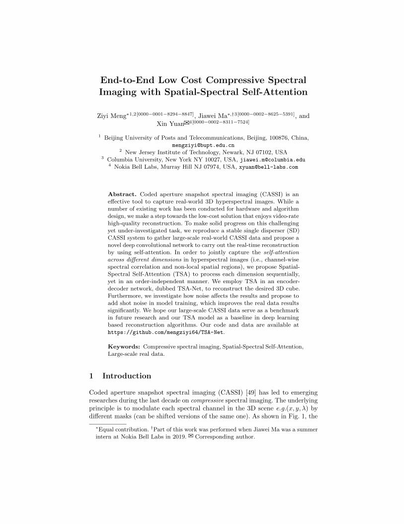
Fig. 2: Real data: The reconstructed hyperspectral video. The video totally contains35 frames (0.028s per frame) captured from our real SD-CASSI system, and each framehas 28 spectral channels between 450 and 650nm. 7 frames and 13 spectral channelsare extracted and shown here. The object is moving from left to right. Please refer tothe video files in the Supplementary Material (SM).

noted above, the imbalanced response and noise are introduced in our collectedreal data, which lead to severe performance degradation compared with thetesting result on simulated noise-free data. This motivated us to employ deeplearning as a tool to mitigate this challenge as well as the slow reconstruction.

Deep learning methods [29,30,52,56] showed the potential to speed up thereconstruction and improve image reconstruction quality. HSSP [52] is a SOTAdeep unfolding method and exploit convolution network to estimate the spatialand spectral priors. Though this has led to promising results, the real data isusually captured by the CASSI system with the expensive direct-view disperser(more than 1000 US dollars based on [50]). In addition, HSSP recovers the wholehyperspectral image based on blocks and may lose non-local information.

Recently, Self-attention mechanism has been proposed in [47] for sequencemodeling tasks such as machine translation, which is able to get rid of thesequence order and model the relationship between each two timestamps inparallel. Multiple heads are considered to model the relationship comprehensively.A limit number of previous work has conducted self-attention to model hyper-spectral image. For instance, λ-Net [29] assumes the spatial correlation foreach channel is shared among all channels and then only considers the spatialcorrelation in a hidden feature space. However, they flatten all features from2D plane into one single dimension to model the spatial correlation, causinghuge memory usage in the attention map calculation. Furthermore, the onlyreal data used in λ-Net [29] is of spatial size 256 × 256, which is a small scaledata. Even though [39] designed an efficient self-attention form to help modelspatial correlation, a strong constrain on the intermediate variables is enforced;


[27] proposed to use a bi-directional Recurrent Neural Network to model thespectral channel correlation but not for CASSI applications. The CDSA in [25]generalized the self-attention where the theoretical analysis shows the order-independent property when applying the dimension-specific attention maps tomodulate the extracted feature map in sequence. Inspired by this, we proposethe Spatial-Spectral Self-Attention (TSA for ‘Triple-S Attention’) and model thespatial-spectral correlation in a joint and order-independent manner. We calculatethe spatial and spectral attention maps separately and use them to modulate thefeature map in sequence, which also maintains reasonable computation complexity.We apply the proposed TSA module in an encoder-decoder network, dubbed asTSA-Net, for CASSI image reconstruction. In addition, we study the effects ofnoise on the reconstruction results and propose to add shot-noise, rather thanGaussian noise, on the clean measurement during training to minimize the gapof performance between simulated noise-free data and real data.

In this paper, we investigate a novel method that can provide high qualityreconstruction for the original and low cost SD-CASSI system, which is reproducedby us and now capable of capturing large-scale data. Our contributions aresummarized as follows:

– We reproduce a stable SD-CASSI system using low-cost components, especiallythe low-cost single disperser, and gather large-scale real CASSI data asbenchmark for future research.

– We propose Spatial-Spectral Self-Attention (TSA) module to model the spatialand spectral correlation in a joint yet order-independent manner with reasonablecomputation cost.

– We employ TSA module in an encoder-decoder network, which can provide660×660×28 spectral cube from a single measurement within 100ms using oneGPU in evaluation. In this manner, we are able to provide a 660×660×28×354D live volume per second with an example shown in Fig. 2.

– We analyse the effect of noises on the reconstruction results and the undesiredhigh frequency details, i.e., artifacts, in the deep learning based reconstruction.We then propose to add shot noise into the training data to simulate the systemenvironment and to mitigate the artifacts in the real hyperspectral image.Experiment comparison shows the performance improvement and network’srobustness, which demonstrates our strategy’s effectiveness.

The rest of this paper is organized as follows: Sec. 2 describes the models ofSD-CASSI.Sec. 3 presents the details of our proposed deep learning based TSA-Net to solve the reconstruction problem of SD-CASSI. Sec. 4 presents extensiveresults on both simulation and real data to demonstrate the superiority of ourproposed TSA-Net as well as the hardware setup. Sec. 5 concludes the paper.

Related Work. Following CASSI, which used a coded aperture and a prismto implement the wavelength modulation, other modulations such as occlusionmask [6], spatial light modulator [70] and digital-micromirror-device [58] have alsobeen used for compressive spectral imaging. Meanwhile, advances of CASSI havealso been developed by using multiple-shots [18], dual-channel [51, 53–55] andhigh-order information [2]. For the reconstruction, various iterative algorithms,


such as TwIST [3], GPSR [11] and GAP-TV [65] have been utilized. Otheralgorithms, such as Gaussian mixture models and sparse coding [37,51, 60] havealso been developed. As mentioned before, most recently, DeSCI proposed in [21]to reconstruct videos or hyperspectral images in snapshot compressive imaginghas led to state-of-the-art results. Inspired by the recent advances of deep learningon image restoration [24, 59, 71], researchers have started using deep learningto reconstruct hyperspectral images from RGB images [1, 19, 20, 31, 40]. Deeplearning models [28,29,52,56] have been developed for CASSI. In addition to thenovel attention-based TSA module in the design, our work differs from previousworks by considering the impact of hardware constraints in CASSI such as realmasks and shot noise.

2 Mathematically Model of SD-CASSI

Model Following the Optical Path. Let F ∈ RNx×Ny×Nλ denote the 3Dspectral cube shown in the left of Fig. 1(c) and M∗ ∈ RNx×Ny denote thephysical mask used for signal modulation. We use F ′ ∈ RNx×Ny×Nλ to representthe modulated signals where images at different wavelengths are modulatedseparately, i.e., for nλ = 1, . . . , Nλ, we have

F ′(:, :, nλ) = F (:, :, nλ)�M∗, (1)

where � represents the element-wise multiplication. After passing the disperser,the cube F ′ is tilted and is considered to be sheared along the y-axis. We thenuse F ′′ ∈ RNx×(Ny+Nλ−1)×Nλ to denote the tilted cube and assume λc to be thereference wavelength, i.e., image F ′(:, :, nλc) is not sheared along the y-axis, wecan have

F ′′(u, v, nλ) = F ′(x, y + d(λn − λc), nλ), (2)

where (u, v) indicates the coordinate system on the detector plane, λn is thewavelength at nλ-th channel and λc denotes the center-wavelength. Then, d(λn−λc) signifies the spatial shifting for nthλ channel. The compressed measurement atthe detector y(u, v) can thus be modelled as

y(u, v) =∫ λmax

λminf ′′(u, v, nλ)dλ, (3)

since the sensor integrates all the light in the wavelength [λmin, λmax], where f ′′

is the analog (continuous) representation of F ′′. In discretized form, the captured2D measurement Y ∈ RNx×(Ny+Nλ−1) is modelled as

Y =∑Nλnλ=1 F

′′(:, :, nλ) +G, (4)

which is a compressed frame contains the information and G ∈ RNx×(Ny+Nλ−1)represents the measurement noise.For the convenience of model description, we further setM ∈ RNx×(Ny+Nλ−1)×Nλto be the shifted version of the mask corresponding to different wavelengths, i.e.,

M(u, v, nλ) = M∗(x, y + d(λn − λc)). (5)


Similarly, for each signal frame at different wavelength, the shifted version isF ∈ RNx×(Ny+Nλ−1)×Nλ ,

F (u, v, nλ) = F (x, y + d(λn − λc), nλ). (6)

Following this, the measurement Y can be represented as

Y =∑Nλnλ=1 F (:, :, nλ)�M(:, :, nλ) +G. (7)

Vectorized Formulation. We use vec(·) to denote the matrix vactorization,i.e., concatenating columns into one vector. Then, we have y = vec(Y ), g =vec(G) ∈ Rn and

f =

f (1)

...

f (Nλ)

∈ RNx(Ny+Nλ−1)Nλ (8)

where n = Nx(Ny +Nλ − 1) and f (nλ) = vec(F (:, :, nλ)),

In addition, we define the sensing matrix as

Φ = [D1, . . . ,DNλ ] ∈ Rn×nNλ , (9)

where Dnλ = Diag(vec(M(:, :, nλ))) is a diagonal matrix with vec(M(:, :, nλ))as the diagonal elements. As such, we then can rewrite the matrix formulation ofEq. (7) as

y = Φf + g. (10)

This is similar to compressive sensing (CS) [9, 10] as Φ is a fat matrix, i.e., morecolumns than rows. However, since Φ has the very special structure as in Eq. (9),most theory developed for CS can not fit in our applications. Note that Φ isa very sparse matrix, i.e., at most nNλ nonzero elements. It has recently beenproved that the signal can still be recovered even when Nλ > 1 [15,16].

After capturing the measurement, the following task is given y (captured bythe camera) and Φ (calibrated based on pre-design), solving f . For the sake ofspeed and quality, we use deep learning to solve this inverse problem.

3 TSA-Net for SD-CASSI Reconstruction

In this section, we first briefly review the conventional self-attention mechanism.Then, we propose Spatial-Spectral Self-Attention module followed by the TSA-Netstructure. In Sec. 3.3, we analysis the effect of noise and discuss the strategy ofinjecting shot noise into simulated measurement during model training, to suppressthe artifacts in the recovered hyperspectral images from real measurementscaptured by our SD-CASSI system. The hardware details can be found in SM.


3.1 Conventional Self-Attention

For self-attention mechanism in [47], given an input sentence of length N , eachtoken xi is mapped into a Query vector qi of f -dim, a Key vector ki of f -dim,and a Value vector vi of v-dim. The attention from token xj to token xi iseffectively the scaled dot-product of qi and kj after Softmax, which is defined as

A(i, j) = exp(S(i,j))∑Nk=1 exp(S(i,k))

where S(i, j) = qik>j /√f . Then, vi is updated to v′i as

a weighted sum of all the Value vectors, defined as v′i =∑Nj=1A(i, j)vj , after

which each v′i is mapped to the layer output x′i of the same size as xi. Meanwhile,a causal constraint is set on the attention maps to force self-attention to learn topredict the next token only from the predicted tokens in translation tasks.

In order to adopt self-attention to jointly model spatial and spectral correlation,the intuitive way is to flatten all pixels into one single dimension and calculatethe attention between each two pixels directly. However, as noted in [29], suchoperation will lead to huge memory usage and limit the effectiveness of correlationmodelling. Instead, our proposed TSA module, described below, can jointly modelspatial and spectral correlation while keep the size of attention map reasonable.

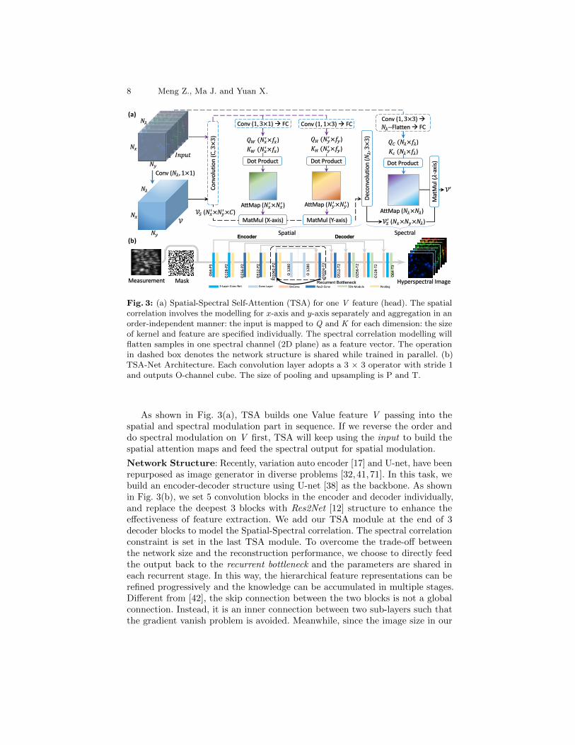
3.2 Spatial-Spectral Self-Attention (TSA)

Spatial Attention: Correlation modelling involves the attention map buildingfor both x-axis and y-axis. We assume the spatial correlation should model thenon-local region information instead of pixel-wise correlation. As a result, a 3× 3convolution kernel is applied to fuse the input feature to indicate the region-basedcorrelation. Then, the convolution net is applied to map the fused feature into Q &K for each dimension individually. The number of kernels effectively denotes thenumber of heads and the kernel size denotes the modulation direction/dimension.Similarly, the dimension-specified Q & K features are used to build the relatedattention maps. TSA uses the dimension-specified attention maps to modulatethe corresponding dimension in sequence while theoretical analysis in [25] hasshown the order-independent property for such operation. The modulated featureare then fed into a deconvolution layer to finish the spatial correlation modelling.Spectral Attention: The samples in the same spectral channel (2D plane) arefirst convolved with one kernel and then flattened into one single dimension,which is set as the feature vector for that channel. Similarly, input feature isthen mapped to Q & K to build the attention map for the spectral axis. Sincethe image patterns on the same position but in two neighboring channels areexpected be highly correlated, we learn to indicate such correlation by settingspectral smoothness on the attention maps. In our proposed model, we normalizeall spectral channel pairwise distances to the range [0, π] and use the cosineof the normalized distance as spectral embedding to indicate channel similarity.Each similarity score is scaled by 0.1 and then added to the coefficients inspectral attention maps, which are then used to modulate Value in self-attentionmodulation. In this way, we induce spectral smoothness constraint since theweights of two adjacent channels in modulation are imposed to be higher thanthose for distant channels (spectral channels with larger wavelength difference).


𝑁!

𝑁"

𝑁#

𝑁!

𝑁"

Conv (𝑁" , 1×1)

𝐼𝑛𝑝𝑢𝑡

𝒱

A)Map (𝑁!$×𝑁!$ ) AttMap (𝑁#$×𝑁#$ )AttMap (𝑁"×𝑁")

Conv (1, 3×3) à𝑁"--Flatten à FC

Conv

olut

ion

(C,3×3)

Deco

nvol

utio

n (𝑁",3×3)

𝒱% (𝑁!$×𝑁#$×𝐶) MatMul (X-axis)

𝑄& (𝑁!$×𝑓!)𝐾& (𝑁!$×𝑓!)

MatMul (Y-axis)

𝑄' (𝑁#$×𝑓#)𝐾' (𝑁#$×𝑓#)

𝑄( (𝑁"×𝑓")𝐾) (𝑁"×𝑓")

𝒱%$ (𝑁!×𝑁#×𝑁")

Mat

Mul

(𝜆-a

xis)

𝒱′

Spatial Spectral

𝑁#Dot Product

Conv (1, 3×1) à FC Conv (1, 1×3) à FC

Dot Product Dot Product

(a)

Measurement Hyperspectral Image

DecoderEncoder

Recurrent Bottleneck

O64

-P3

Res2-Conv PoolingTSA-Module3-Layer Conv Net Conv Layer DeConv

Mask

O12

8-P2

O25

6-P2

O51

2-P2

O10

42-P

2

O 1

280

O 1

280

O10

24-T

2

O51

2-T2

O25

6-T2

O12

8-T2

O64

-T3

(b)

Fig. 3: (a) Spatial-Spectral Self-Attention (TSA) for one V feature (head). The spatialcorrelation involves the modelling for x-axis and y-axis separately and aggregation in anorder-independent manner: the input is mapped to Q and K for each dimension: the sizeof kernel and feature are specified individually. The spectral correlation modelling willflatten samples in one spectral channel (2D plane) as a feature vector. The operationin dashed box denotes the network structure is shared while trained in parallel. (b)TSA-Net Architecture. Each convolution layer adopts a 3 × 3 operator with stride 1and outputs O-channel cube. The size of pooling and upsampling is P and T.

As shown in Fig. 3(a), TSA builds one Value feature V passing into thespatial and spectral modulation part in sequence. If we reverse the order anddo spectral modulation on V first, TSA will keep using the input to build thespatial attention maps and feed the spectral output for spatial modulation.

Network Structure: Recently, variation auto encoder [17] and U-net, have beenrepurposed as image generator in diverse problems [32,41,71]. In this task, webuild an encoder-decoder structure using U-net [38] as the backbone. As shownin Fig. 3(b), we set 5 convolution blocks in the encoder and decoder individually,and replace the deepest 3 blocks with Res2Net [12] structure to enhance theeffectiveness of feature extraction. We add our TSA module at the end of 3decoder blocks to model the Spatial-Spectral correlation. The spectral correlationconstraint is set in the last TSA module. To overcome the trade-off betweenthe network size and the reconstruction performance, we choose to directly feedthe output back to the recurrent bottleneck and the parameters are shared ineach recurrent stage. In this way, the hierarchical feature representations can berefined progressively and the knowledge can be accumulated in multiple stages.Different from [42], the skip connection between the two blocks is not a globalconnection. Instead, it is an inner connection between two sub-layers such thatthe gradient vanish problem is avoided. Meanwhile, since the image size in our


Ground Truth (a) Clean (b) w/ Gaussian noise (c) w/ Shot noise

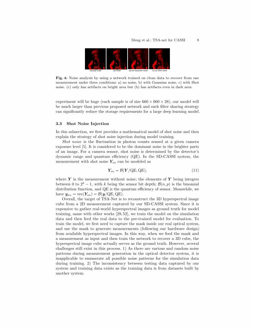
Fig. 4: Noise analysis by using a network trained on clean data to recover from onemeasurement under three conditions: a) no noise, b) with Gaussian noise, c) with Shotnoise. (c) only has artifacts on bright area but (b) has artifacts even in dark area.

experiment will be huge (each sample is of size 660× 660× 28), our model willbe much larger than previous proposed network and such filter sharing strategycan significantly reduce the storage requirements for a large deep learning model.

3.3 Shot Noise Injection

In this subsection, we first provides a mathematical model of shot noise and thenexplain the strategy of shot noise injection during model training.

Shot noise is the fluctuation in photon counts sensed at a given cameraexposure level [5]. It is considered to be the dominant noise in the brighter partsof an image. For a camera sensor, shot noise is determined by the detector’sdynamic range and quantum efficiency (QE). In the SD-CASSI system, themeasurement with shot noise Ysn can be modeled as

Ysn = B(Y /QE,QE), (11)

where Y is the measurement without noise; the elements of Y being integersbetween 0 to 2k − 1, with k being the sensor bit depth; B(n, p) is the binomialdistribution function, and QE is the quantum efficiency of sensor. Meanwhile, wehave ysn = vec(Ysn) = B(y/QE,QE).

Overall, the target of TSA-Net is to reconstruct the 3D hyperspectral imagecube from a 2D measurement captured by our SD-CASSI system. Since it isexpensive to gather real-world hyperspectral images as ground truth for modeltraining, same with other works [29,52], we train the model on the simulationdata and then feed the real data to the pre-trained model for evaluation. Totrain the model, we first need to capture the mask inside our real optical system,and use the mask to generate measurements (following our hardware design)from available hyperspectral images. In this way, when we feed the mask anda measurement as input and then train the network to recover a 3D cube, thehyperspectral image cube actually serves as the ground truth. However, severalchallenges still exist in this process. 1) As there are various and random noisepatterns during measurement generation in the optical detector system, it isinapplicable to enumerate all possible noise patterns for the simulation dataduring training. 2) The inconsistency between testing data captured by oursystem and training data exists as the training data is from datasets built byanother system.


Fig. 5: 10 testing scenes used in simulation.

As such, there is severe performance degradation of reconstruction and theartifacts caused by system noise are obvious during testing. 3) Factors such asresponse imbalance caused by single disperser will lead to poor system calibration.

To overcome these challenges and enhance the model’s robustness, previousworks have adopted various techniques during model training, e.g., addingGaussian noise [4, 48] in the network bottleneck and image augmentation [33].However, a large amount of samples are required during training to learn noisedrawn from Gaussian distributions of all possible hyper-parameters. In contrast,each shot noise value depends on the signal level at each pixel. Besides, shot noiseis usually dominant in an imaging system like our system with bright illuminationand high exposure [26]. To analyse the link between noise in hardware systemand reconstruction artifacts, we compare the reconstruction results in simulationand real data. As shown in Fig. 4, for a network trained by clean data, thereconstruction of measurement with shot noise (right-most column) has artifactsin the object area, which is similar to real data (top in Fig. 12), while the artifactsdistribute in the whole region in the result of measurement with Gaussian noise.

As a result, we propose to add shot noise to the clean measurement duringmodel training (i.e., using Φ>ysn as the input of the TSA-Net) and we findreconstruction performance degradation between the simulation and real datacaptured by hardware system is narrowed. We have also observed this in othersnapshot compressive imaging systems [7, 22, 23, 28, 34–36, 43–46, 63, 64, 66–69]and our proposed TSA-Net can be extended to those systems.

4 Experiments

In Sec. 4.1, we evaluate the reconstruction performance on the synthetic datain simulation. In Sec. 4.2, we demonstrate experimental results captured byour SD-CASSI system. The performance comparison is provided to show theeffectiveness of network and our training strategy.

4.1 Simulation

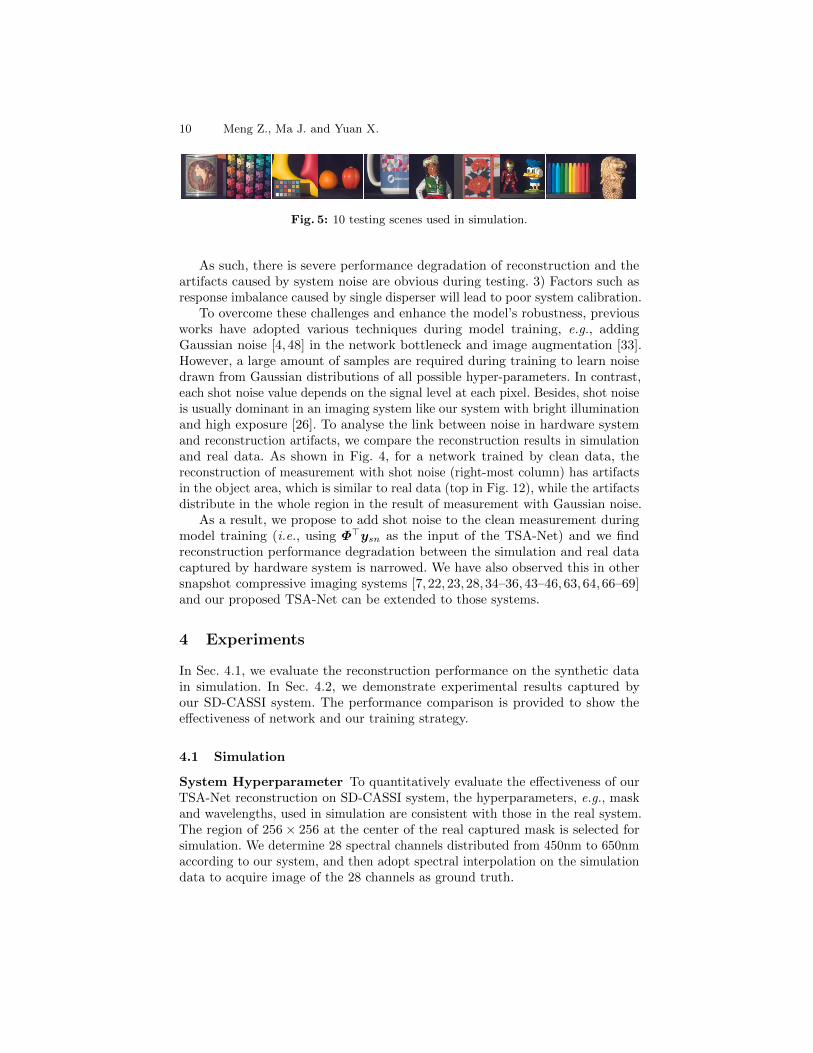
System Hyperparameter To quantitatively evaluate the effectiveness of ourTSA-Net reconstruction on SD-CASSI system, the hyperparameters, e.g., maskand wavelengths, used in simulation are consistent with those in the real system.The region of 256× 256 at the center of the real captured mask is selected forsimulation. We determine 28 spectral channels distributed from 450nm to 650nmaccording to our system, and then adopt spectral interpolation on the simulationdata to acquire image of the 28 channels as ground truth.


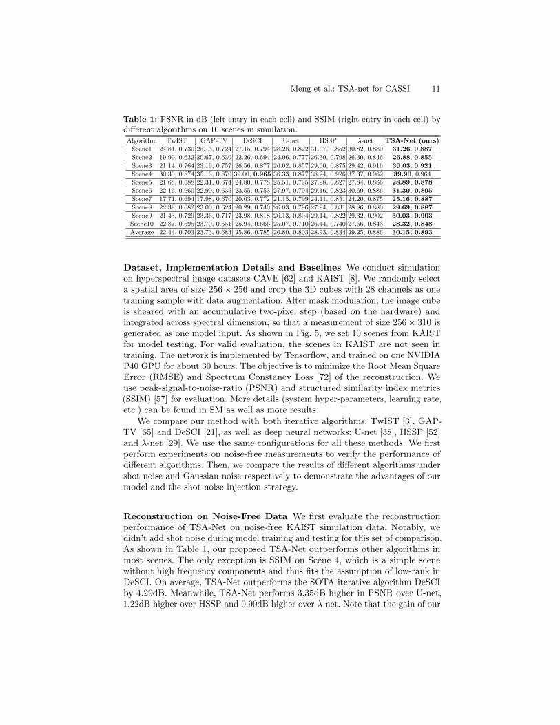
Table 1: PSNR in dB (left entry in each cell) and SSIM (right entry in each cell) bydifferent algorithms on 10 scenes in simulation.

Algorithm TwIST GAP-TV DeSCI U-net HSSP λ-net TSA-Net (ours)

Scene1 24.81, 0.730 25.13, 0.724 27.15, 0.794 28.28, 0.822 31.07, 0.852 30.82, 0.880 31.26, 0.887

Scene2 19.99, 0.632 20.67, 0.630 22.26, 0.694 24.06, 0.777 26.30, 0.798 26.30, 0.846 26.88, 0.855

Scene3 21.14, 0.764 23.19, 0.757 26.56, 0.877 26.02, 0.857 29.00, 0.875 29.42, 0.916 30.03, 0.921

Scene4 30.30, 0.874 35.13, 0.870 39.00, 0.965 36.33, 0.877 38.24, 0.926 37.37, 0.962 39.90, 0.964

Scene5 21.68, 0.688 22.31, 0.674 24.80, 0.778 25.51, 0.795 27.98, 0.827 27.84, 0.866 28.89, 0.878

Scene6 22.16, 0.660 22.90, 0.635 23.55, 0.753 27.97, 0.794 29.16, 0.823 30.69, 0.886 31.30, 0.895

Scene7 17.71, 0.694 17.98, 0.670 20.03, 0.772 21.15, 0.799 24.11, 0.851 24.20, 0.875 25.16, 0.887

Scene8 22.39, 0.682 23.00, 0.624 20.29, 0.740 26.83, 0.796 27.94, 0.831 28.86, 0.880 29.69, 0.887

Scene9 21.43, 0.729 23.36, 0.717 23.98, 0.818 26.13, 0.804 29.14, 0.822 29.32, 0.902 30.03, 0.903

Scene10 22.87, 0.595 23.70, 0.551 25.94, 0.666 25.07, 0.710 26.44, 0.740 27.66, 0.843 28.32, 0.848

Average 22.44, 0.703 23.73, 0.683 25.86, 0.785 26.80, 0.803 28.93, 0.834 29.25, 0.886 30.15, 0.893

Dataset, Implementation Details and Baselines We conduct simulationon hyperspectral image datasets CAVE [62] and KAIST [8]. We randomly selecta spatial area of size 256× 256 and crop the 3D cubes with 28 channels as onetraining sample with data augmentation. After mask modulation, the image cubeis sheared with an accumulative two-pixel step (based on the hardware) andintegrated across spectral dimension, so that a measurement of size 256× 310 isgenerated as one model input. As shown in Fig. 5, we set 10 scenes from KAISTfor model testing. For valid evaluation, the scenes in KAIST are not seen intraining. The network is implemented by Tensorflow, and trained on one NVIDIAP40 GPU for about 30 hours. The objective is to minimize the Root Mean SquareError (RMSE) and Spectrum Constancy Loss [72] of the reconstruction. Weuse peak-signal-to-noise-ratio (PSNR) and structured similarity index metrics(SSIM) [57] for evaluation. More details (system hyper-parameters, learning rate,etc.) can be found in SM as well as more results.

We compare our method with both iterative algorithms: TwIST [3], GAP-TV [65] and DeSCI [21], as well as deep neural networks: U-net [38], HSSP [52]and λ-net [29]. We use the same configurations for all these methods. We firstperform experiments on noise-free measurements to verify the performance ofdifferent algorithms. Then, we compare the results of different algorithms undershot noise and Gaussian noise respectively to demonstrate the advantages of ourmodel and the shot noise injection strategy.

Reconstruction on Noise-Free Data We first evaluate the reconstructionperformance of TSA-Net on noise-free KAIST simulation data. Notably, wedidn’t add shot noise during model training and testing for this set of comparison.As shown in Table 1, our proposed TSA-Net outperforms other algorithms inmost scenes. The only exception is SSIM on Scene 4, which is a simple scenewithout high frequency components and thus fits the assumption of low-rank inDeSCI. On average, TSA-Net outperforms the SOTA iterative algorithm DeSCIby 4.29dB. Meanwhile, TSA-Net performs 3.35dB higher in PSNR over U-net,1.22dB higher over HSSP and 0.90dB higher over λ-net. Note that the gain of our


Truth

TwIST

GAP-TV

HSSP

-net

TSA-net

462.1 nm 551.4 nm 594.4 nm 636.3 nmMeasurement

DeSCI

a

b

RGB image

Truth HSSP -net TSA-net

Truth462.1 nm 551.4 nm 594.4 nmMeasurement

TwIST

GAP-TV

HSSP

-net

TSA-net

Truth HSSP

DeSCI

a

b

RGB image

-net TSA-net

636.3 nm

(b)

(a)(a)

(b)

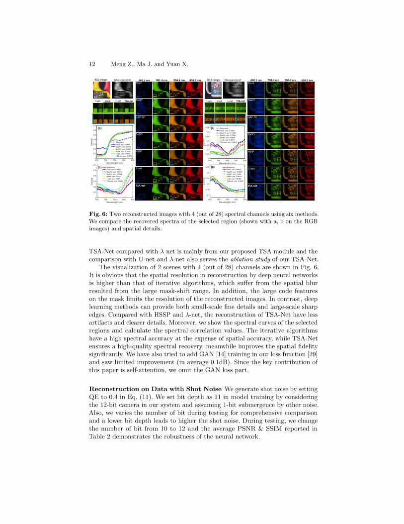
Fig. 6: Two reconstructed images with 4 (out of 28) spectral channels using six methods.We compare the recovered spectra of the selected region (shown with a, b on the RGBimages) and spatial details.

TSA-Net compared with λ-net is mainly from our proposed TSA module and thecomparison with U-net and λ-net also serves the ablation study of our TSA-Net.

The visualization of 2 scenes with 4 (out of 28) channels are shown in Fig. 6.It is obvious that the spatial resolution in reconstruction by deep neural networksis higher than that of iterative algorithms, which suffer from the spatial blurresulted from the large mask-shift range. In addition, the large code featureson the mask limits the resolution of the reconstructed images. In contrast, deeplearning methods can provide both small-scale fine details and large-scale sharpedges. Compared with HSSP and λ-net, the reconstruction of TSA-Net have lessartifacts and clearer details. Moreover, we show the spectral curves of the selectedregions and calculate the spectral correlation values. The iterative algorithmshave a high spectral accuracy at the expense of spatial accuracy, while TSA-Netensures a high-quality spectral recovery, meanwhile improves the spatial fidelitysignificantly. We have also tried to add GAN [14] training in our loss function [29]and saw limited improvement (in average 0.1dB). Since the key contribution ofthis paper is self-attention, we omit the GAN loss part.

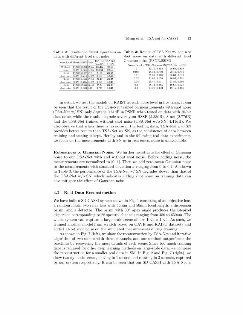
Reconstruction on Data with Shot Noise We generate shot noise by settingQE to 0.4 in Eq. (11). We set bit depth as 11 in model training by consideringthe 12-bit camera in our system and assuming 1-bit submergence by other noise.Also, we varies the number of bit during testing for comprehensive comparisonand a lower bit depth leads to higher the shot noise. During testing, we changethe number of bit from 10 to 12 and the average PSNR & SSIM reported inTable 2 demonstrates the robustness of the neural network.


Table 2: Results of different algorithms ondata with different level shot noise

Noise Level Metric HSSP λ-netTSA-Netw/o SN

TSA-Netw/ SN

Without PSNR 28.93 29.25 30.15 28.69noise SSIM 0.834 0.886 0.893 0.859

12-bit PSNR 25.87 27.91 28.36 28.55shot noise SSIM 0.744 0.822 0.850 0.856



Table 3: Results of TSA-Net w/ and w/oshot noise on data with different levelGaussian noise (PSNR,SSIM)

Noise Level σ TSA-Net w/o SN TSA-Net w/ SN

0 30.15, 0.893 28.69, 0.8590.005 28.33, 0.830 28.46, 0.8360.01 25.39, 0.778 28.03, 0.8190.02 22.65, 0.658 26.93, 0.7810.05 19.47, 0.541 23.50, 0.6600.1 18.74, 0.485 19.67, 0.5280.2 18.20, 0.443 19.15, 0.468

In detail, we test the models on KAIST at each noise level in five trials. It canbe seen that the result of the TSA-Net trained on measurements with shot noise(TSA-Net w/ SN) only degrade 0.61dB in PSNR when tested on data with 10-bitshot noise, while the results degrade severely on HSSP (5.33dB), λ-net (2.77dB)and the TSA-Net trained without shot noise (TSA-Net w/o SN, 4.41dB). Wealso observe that when there is no noise in the testing data, TSA-Net w/o SNprovides better results than TSA-Net w/ SN, as the consistence of data betweentraining and testing is kept. Hereby and in the following real data experiments,we focus on the measurements with SN as in real cases, noise is unavoidable.

Robustness to Gaussian Noise. We further investigate the effect of Gaussiannoise to our TSA-Net with and without shot noise. Before adding noise, themeasurements are normalized to [0, 1]. Then we add zero-mean Gaussian noiseto the measurements with standard deviation σ ranging from 0 to 0.2. As shownin Table 3, the performance of the TSA-Net w/ SN degrades slower than that ofthe TSA-Net w/o SN, which indicates adding shot noise on training data canalso mitigate the effect of Gaussian noise.

4.2 Real Data Reconstruction

We have built a SD-CASSI system shown in Fig. 1 consisting of an objective lens,a random mask, two relay lens with 45mm and 50mm focal length, a dispersionprism, and a detector. The prism with 30◦ apex angle produces the 54-pixeldispersion corresponding to 28 spectral channels ranging from 450 to 650nm. Thewhole system can capture a large-scale scene of size 1024 × 1024. As such, wetrained another model from scratch based on CAVE and KAIST datasets andadded 11-bit shot noise on the simulated measurements during training.

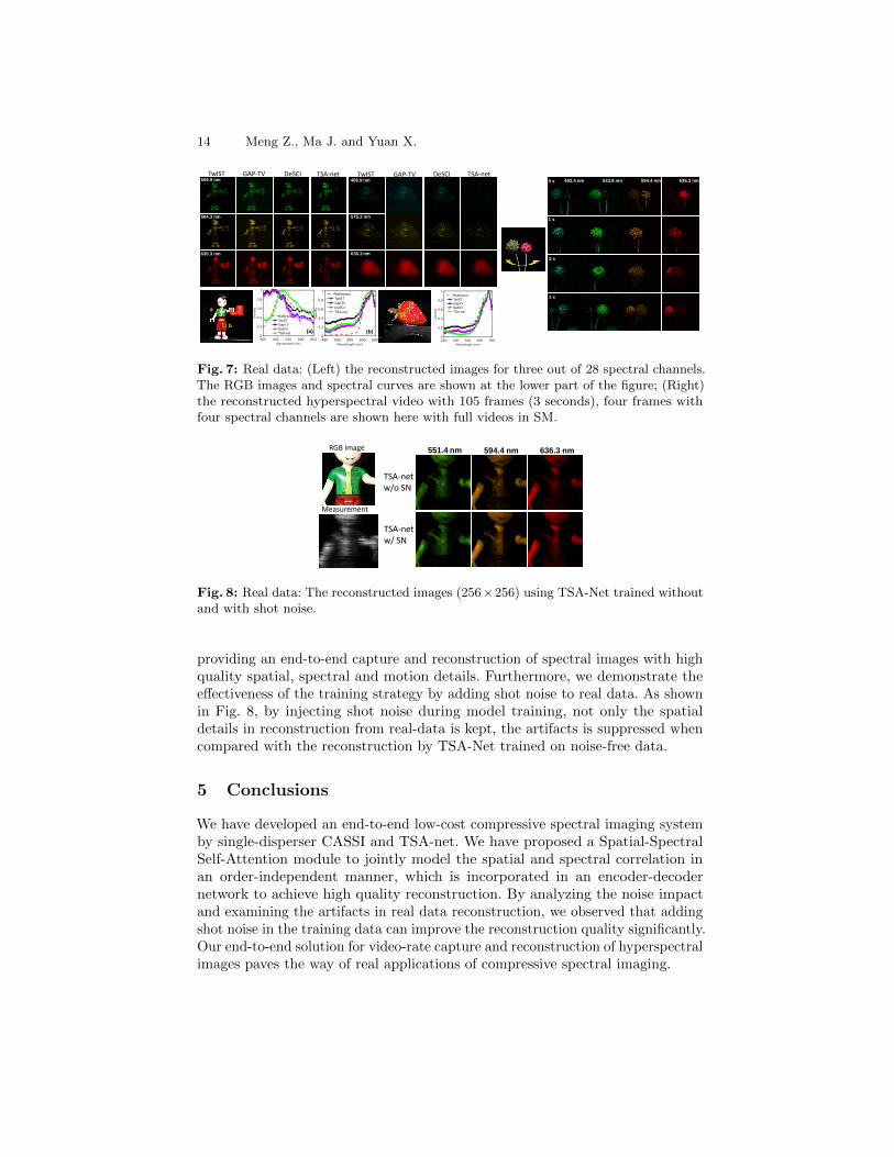
As shown in Fig. 7 (left), we show the reconstruction by TSA-Net and iterativealgorithm of two scenes with three channels, and our method outperforms thebaselines by recovering the most details of each scene. Since too much trainingtime is required for other deep learning methods on large-scale data, we comparethe reconstruction for a smaller real data in SM. In Fig. 2 and Fig. 7 (right), weshow two dynamic scenes, moving in 1 second and rotating in 3 seconds, capturedby our system respectively. It can be seen that our SD-CASSI with TSA-Net is


a

b

TwIST GAP-TV DeSCI TwIST GAP-TV DeSCI TSA-net0 s 594.4 nm 636.3 nm492.4 nm 543.8 nm

1 s

2 s

3 s

509.9 nm

584.3 nm

636.3 nm

486.9 nm

575.3 nm

636.3 nm

(a) (b)

TSA-net

Fig. 7: Real data: (Left) the reconstructed images for three out of 28 spectral channels.The RGB images and spectral curves are shown at the lower part of the figure; (Right)the reconstructed hyperspectral video with 105 frames (3 seconds), four frames withfour spectral channels are shown here with full videos in SM.

TSA-netw/o SN

TSA-net w/ SN

551.4 nm 594.4 nm 636.3 nm

Measurement

RGB image

Fig. 8: Real data: The reconstructed images (256×256) using TSA-Net trained withoutand with shot noise.

providing an end-to-end capture and reconstruction of spectral images with highquality spatial, spectral and motion details. Furthermore, we demonstrate theeffectiveness of the training strategy by adding shot noise to real data. As shownin Fig. 8, by injecting shot noise during model training, not only the spatialdetails in reconstruction from real-data is kept, the artifacts is suppressed whencompared with the reconstruction by TSA-Net trained on noise-free data.

5 Conclusions

We have developed an end-to-end low-cost compressive spectral imaging systemby single-disperser CASSI and TSA-net. We have proposed a Spatial-SpectralSelf-Attention module to jointly model the spatial and spectral correlation inan order-independent manner, which is incorporated in an encoder-decodernetwork to achieve high quality reconstruction. By analyzing the noise impactand examining the artifacts in real data reconstruction, we observed that addingshot noise in the training data can improve the reconstruction quality significantly.Our end-to-end solution for video-rate capture and reconstruction of hyperspectralimages paves the way of real applications of compressive spectral imaging.


References

1. Akhtar, N., Mian, A.S.: Hyperspectral recovery from rgb images using gaussianprocesses. IEEE transactions on pattern analysis and machine intelligence (2018)

2. Arguello, H., Rueda, H., Wu, Y., Prather, D.W., Arce, G.R.: Higher-ordercomputational model for coded aperture spectral imaging. Appl. Opt. 52(10),D12–D21 (Apr 2013)

3. Bioucas-Dias, J., Figueiredo, M.: A new TwIST: Two-step iterativeshrinkage/thresholding algorithms for image restoration. IEEE Transactions onImage Processing 16(12), 2992–3004 (December 2007)

4. Bishop, C.M.: Training with noise is equivalent to tikhonov regularization. Neuralcomputation 7(1), 108–116 (1995)

5. Blanter, Y.M., Buttiker, M.: Shot noise in mesoscopic conductors. Physics reports336(1-2), 1–166 (2000)

6. Cao, X., Du, H., Tong, X., Dai, Q., Lin, S.: A prism-mask system for multispectralvideo acquisition. IEEE transactions on pattern analysis and machine intelligence33(12), 2423–2435 (2011)

7. Cheng, Z., Lu, R., Wang, Z., Zhang, H., Chen, B., Meng, Z., Yuan, X.: BIRNAT:Bidirectional Recurrent Neural Networks with Adversarial Training for VideoSnapshot Compressive Imaging. In: European Conference on Computer Vision(ECCV) (August 2020)

8. Choi, I., Jeon, D.S., Nam, G., Gutierrez, D., Kim, M.H.: High-quality hyperspectralreconstruction using a spectral prior. vol. 36, p. 218. ACM (2017)

9. Donoho, D.L.: Compressed sensing. IEEE Transactions on Information Theory52(4), 1289–1306 (April 2006)

10. Emmanuel, C., Romberg, J., Tao, T.: Robust uncertainty principles: Exact signalreconstruction from highly incomplete frequency information. IEEE Transactionson Information Theory 52(2), 489–509 (February 2006)

11. Figueiredo, M.A., Nowak, R.D., Wright, S.J.: Gradient projection for sparsereconstruction: Application to compressed sensing and other inverse problems.IEEE Journal of selected topics in signal processing 1(4), 586–597 (2007)

12. Gao, S.H., Cheng, M.M., Zhao, K., Zhang, X.Y., Yang, M.H., Torr, P.: Res2net: Anew multi-scale backbone architecture (2019)

13. Gehm, M.E., John, R., Brady, D.J., Willett, R.M., Schulz, T.J.: Single-shotcompressive spectral imaging with a dual-disperser architecture. Optics Express15(21), 14013–14027 (2007)

14. Goodfellow, I.J., Pouget-Abadie, J., Mirza, M., Xu, B., Warde-Farley, D., Ozair, S.,Courville, A., Bengio, Y.: Generative adversarial nets. In: Proceedings of the 27thInternational Conference on Neural Information Processing Systems - Volume 2.pp. 2672–2680. NIPS’14 (2014)

15. Jalali, S., Yuan, X.: Compressive imaging via one-shot measurements. In: IEEEInternational Symposium on Information Theory (ISIT) (2018)

16. Jalali, S., Yuan, X.: Snapshot compressed sensing: Performance bounds andalgorithms. IEEE Transactions on Information Theory 65(12), 8005–8024 (Dec2019)

17. Kingma, D.P., Welling, M.: Auto-encoding variational bayes (2013), citearxiv:1312.6114

18. Kittle, D., Choi, K., Wagadarikar, A., Brady, D.J.: Multiframe image estimationfor coded aperture snapshot spectral imagers. Applied Optics 49(36), 6824–6833(December 2010)


19. Koundinya, S., Sharma, H., Sharma, M., Upadhyay, A., Manekar, R., Mukhopadhyay,R., Karmakar, A., Chaudhury, S.: 2d-3d cnn based architectures for spectralreconstruction from rgb images. In: The IEEE Conference on Computer Vision andPattern Recognition (CVPR) Workshops (June 2018)

20. Li, H., Xiong, Z., Shi, Z., Wang, L., Liu, D., Wu, F.: Hsvcnn: Cnn-basedhyperspectral reconstruction from rgb videos. In: 2018 25th IEEE InternationalConference on Image Processing (ICIP). pp. 3323–3327 (Oct 2018)

21. Liu, Y., Yuan, X., Suo, J., Brady, D.J., Dai, Q.: Rank minimization for snapshotcompressive imaging. IEEE Transactions on Pattern Analysis and MachineIntelligence 41(12), 2990–3006 (Dec 2019)

22. Llull, P., Liao, X., Yuan, X., Yang, J., Kittle, D., Carin, L., Sapiro, G., Brady, D.J.:Coded aperture compressive temporal imaging. Optics Express 21(9), 10526–10545(2013)

23. Llull, P., Yuan, X., Carin, L., Brady, D.J.: Image translation for single-shot focaltomography. Optica 2(9), 822–825 (2015)

24. Ma, J., Liu, X., Shou, Z., Yuan, X.: Deep tensor admm-net for snapshot compressiveimaging. In: IEEE/CVF Conference on Computer Vision (ICCV) (2019)

25. Ma, J., Shou, Z., Zareian, A., Mansour, H., Vetro, A., Chang, S.F.: Cdsa: Cross-dimensional self-attention for multivariate, geo-tagged time series imputation. arXivpreprint arXiv:1905.09904 (2019)

26. MacDonald, L.: Digital heritage. Routledge (2006)27. Mei, X., Pan, E., Ma, Y., Dai, X., Huang, J., Fan, F., Du, Q., Zheng, H., Ma, J.:

Spectral-spatial attention networks for hyperspectral image classification. RemoteSensing 11(8), 963 (2019)

28. Meng, Z., Qiao, M., Ma, J., Yu, Z., Xu, K., Yuan, X.: Snapshot multispectralendomicroscopy. Opt. Lett. 45(14), 3897–3900 (Jul 2020)

29. Miao, X., Yuan, X., Pu, Y., Athitsos, V.: λ-net: Reconstruct hyperspectral imagesfrom a snapshot measurement. In: IEEE/CVF Conference on Computer Vision(ICCV) (2019)

30. Miao, X., Yuan, X., Wilford, P.: Deep learning for compressive spectral imaging.In: Digital Holography and Three-Dimensional Imaging 2019. p. M3B.3. OpticalSociety of America (2019)

31. Nie, S., Gu, L., Zheng, Y., Lam, A., Ono, N., Sato, I.: Deeply learned filter responsefunctions for hyperspectral reconstruction. In: The IEEE Conference on ComputerVision and Pattern Recognition (CVPR) (June 2018)

32. Peng, P., Jalali, S., Yuan, X.: Solving inverse problems via auto-encoders. IEEEJournal on Selected Areas in Information Theory 1(1), 312–323 (2020)

33. Perez, L., Wang, J.: The effectiveness of data augmentation in image classificationusing deep learning. arXiv preprint arXiv:1712.04621 (2017)

34. Qiao, M., Liu, X., Yuan, X.: Snapshot spatial–temporal compressive imaging. Opt.Lett. 45(7), 1659–1662 (Apr 2020)

35. Qiao, M., Meng, Z., Ma, J., Yuan, X.: Deep learning for video compressive sensing.APL Photonics 5(3), 030801 (2020)

36. Qiao, M., Sun, Y., Liu, X., Yuan, X., Wilford, P.: Snapshot optical coherencetomography. In: Digital Holography and Three-Dimensional Imaging 2019. p. W4B.3.Optical Society of America (2019)

37. Renna, F., Wang, L., Yuan, X., Yang, J., Reeves, G., Calderbank, R., Carin, L.,Rodrigues, M.R.: Classification and reconstruction of high-dimensional signals fromlow-dimensional features in the presence of side information. IEEE Transactions onInformation Theory 62(11), 6459–6492 (2016)


38. Ronneberger, O., Fischer, P., Brox, T.: U-net: Convolutional networks for biomedicalimage segmentation. In: International Conference on Medical image computing andcomputer-assisted intervention. pp. 234–241. Springer (2015)

39. Shen, Z., Zhang, M., Zhao, H., Yi, S., Li, H.: Efficient attention: Attention withlinear complexities. arXiv preprint arXiv:1812.01243 (2018)

40. Shi, Z., Chen, C., Xiong, Z., Liu, D., Wu, F.: Hscnn+: Advanced cnn-basedhyperspectral recovery from rgb images. In: The IEEE Conference on ComputerVision and Pattern Recognition (CVPR) Workshops (June 2018)

41. Sinha, A., Lee, J., Li, S., Barbastathis, G.: Lensless computational imaging throughdeep learning. Optica 4(9), 1117–1125 (Sep 2017)

42. Sun, L., Fan, Z., Huang, Y., Ding, X., Paisley, J.: Compressed sensing mri usinga recursive dilated network. In: Thirty-Second AAAI Conference on ArtificialIntelligence (2018)

43. Sun, Y., Yuan, X., Pang, S.: High-speed compressive range imaging based on activeillumination. Optics Express 24(20), 22836–22846 (Oct 2016)

44. Sun, Y., Yuan, X., Pang, S.: Compressive high-speed stereo imaging. Opt Express25(15), 18182–18190 (2017)

45. Tsai, T.H., Llull, P., Yuan, X., Carin, L., Brady, D.J.: Spectral-temporal compressiveimaging. Optics Letters 40(17), 4054–4057 (Sep 2015)

46. Tsai, T.H., Yuan, X., Brady, D.J.: Spatial light modulator based color polarizationimaging. Optics Express 23(9), 11912–11926 (May 2015)

47. Vaswani, A., Shazeer, N., Parmar, N., Uszkoreit, J., Jones, L., Gomez, A.N., Kaiser, L., Polosukhin, I.: Attention is all you need. In: Advances in neural informationprocessing systems. pp. 5998–6008 (2017)

48. Vincent, P., Larochelle, H., Lajoie, I., Bengio, Y., Manzagol, P.A.: Stacked denoisingautoencoders: Learning useful representations in a deep network with a localdenoising criterion. Journal of machine learning research 11(Dec), 3371–3408 (2010)

49. Wagadarikar, A., John, R., Willett, R., Brady, D.: Single disperser design for codedaperture snapshot spectral imaging. Applied Optics 47(10), B44–B51 (2008)

50. Wagadarikar, A.A., Pitsianis, N.P., Sun, X., Brady, D.J.: Video rate spectral imagingusing a coded aperture snapshot spectral imager. Optics Express 17(8), 6368–6388(2009)

51. Wang, L., Xiong, Z., Shi, G., Wu, F., Zeng, W.: Adaptive nonlocal sparserepresentation for dual-camera compressive hyperspectral imaging. IEEETransactions on Pattern Analysis and Machine Intelligence 39(10), 2104–2111(Oct 2017)

52. Wang, L., Sun, C., Fu, Y., Kim, M.H., Huang, H.: Hyperspectral imagereconstruction using a deep spatial-spectral prior. In: The IEEE Conference onComputer Vision and Pattern Recognition (CVPR) (June 2019)

53. Wang, L., Xiong, Z., Gao, D., Shi, G., Wu, F.: Dual-camera design for codedaperture snapshot spectral imaging. Appl. Opt. 54(4), 848–858 (Feb 2015)

54. Wang, L., Xiong, Z., Gao, D., Shi, G., Zeng, W., Wu, F.: High-speed hyperspectralvideo acquisition with a dual-camera architecture. In: 2015 IEEE Conference onComputer Vision and Pattern Recognition (CVPR). pp. 4942–4950 (June 2015)

55. Wang, L., Xiong, Z., Huang, H., Shi, G., Wu, F., Zeng, W.: High-speedhyperspectral video acquisition by combining nyquist and compressive sampling.IEEE Transactions on Pattern Analysis and Machine Intelligence (2018)

56. Wang, L., Zhang, T., Fu, Y., Huang, H.: Hyperreconnet: Joint coded apertureoptimization and image reconstruction for compressive hyperspectral imaging. IEEETransactions on Image Processing 28(5), 2257–2270 (May 2019)


57. Wang, Z., Bovik, A.C., Sheikh, H.R., Simoncelli, E.P., et al.: Image qualityassessment: From error visibility to structural similarity. IEEE Transactions onImage Processing 13(4), 600–612 (2004)

58. Wu, Y., Mirza, I.O., Arce, G.R., Prather, D.W.: Development of a digital-micromirror-device-based multishot snapshot spectral imaging system. Opt. Lett.36(14), 2692–2694 (Jul 2011)

59. Xie, J., Xu, L., Chen, E.: Image denoising and inpainting with deep neural networks.In: Pereira, F., Burges, C.J.C., Bottou, L., Weinberger, K.Q. (eds.) Advances inNeural Information Processing Systems 25, pp. 341–349. Curran Associates, Inc.(2012)

60. Yang, J., Liao, X., Yuan, X., Llull, P., Brady, D.J., Sapiro, G., Carin, L.:Compressive sensing by learning a Gaussian mixture model from measurements.IEEE Transaction on Image Processing 24(1), 106–119 (January 2015)

61. Yang, P., Kong, L., Liu, X., Yuan, X., Chen, G.: Shearlet enhanced snapshotcompressive imaging. IEEE Transactions on Image Processing 29, 6466–6481 (2020)

62. Yasuma, F., Mitsunaga, T., Iso, D., Nayar, S.K.: Generalized assorted pixel camera:postcapture control of resolution, dynamic range, and spectrum. vol. 19, pp. 2241–2253. IEEE (2010)

63. Yuan, X., Sun, Y., Pang, S.: Efficient patch-based approach for compressive depthimaging. Appl. Opt. 56(10), 2697–2704 (2017)

64. Yuan, X.: Compressive dynamic range imaging via Bayesian shrinkage dictionarylearning. Optical Engineering 55(12), 123110 (2016)

65. Yuan, X.: Generalized alternating projection based total variation minimization forcompressive sensing. In: 2016 IEEE International Conference on Image Processing(ICIP). pp. 2539–2543 (Sept 2016)

66. Yuan, X., Brady, D., Katsaggelos, A.K.: Snapshot compressive imaging: Theory,algorithms and applications. IEEE Signal Processing Magazine (2020)

67. Yuan, X., Liao, X., Llull, P., Brady, D., Carin, L.: Efficient patch-based approachfor compressive depth imaging. Applied Optics 55(27), 7556–7564 (Sep 2016)

68. Yuan, X., Llull, P., Liao, X., Yang, J., Brady, D.J., Sapiro, G., Carin, L.: Low-costcompressive sensing for color video and depth. In: IEEE Conference on ComputerVision and Pattern Recognition (CVPR). pp. 3318–3325 (2014)

69. Yuan, X., Pang, S.: Structured illumination temporal compressive microscopy.Biomedical Optics Express 7, 746–758 (2016)

70. Yuan, X., Tsai, T.H., Zhu, R., Llull, P., Brady, D., Carin, L.: Compressivehyperspectral imaging with side information. IEEE Journal of Selected Topicsin Signal Processing 9(6), 964–976 (September 2015)

71. Zhang, K., Zuo, W., Chen, Y., Meng, D., Zhang, L.: Beyond a gaussian denoiser:Residual learning of deep cnn for image denoising. IEEE Transactions on ImageProcessing 26(7), 3142–3155 (July 2017)

72. Zhao, Y., Guo, H., Ma, Z., Cao, X., Yue, T., Hu, X.: Hyperspectral imaging withrandom printed mask. In: Proceedings of the IEEE Conference on Computer Visionand Pattern Recognition. pp. 10149–10157 (2019)

End-to-End Low Cost Compressive Spectral Imaging with ...

Documents

Transcript of End-to-End Low Cost Compressive Spectral Imaging with ...