1

Employee Relationship and Earnings Management

Abstract:

This paper examines the association between a firm’s relationship with its employees and

the extent of earnings management. We find that firms with friendly employee relationship (as

measured by the Employee Relations Index) have more earnings management, particularly in

the form of income-decreasing earnings management. Further analysis shows that cash profit

sharing is the most important component in the Employee Relations Index in determining our

results since managers tend to manipulate earnings downward to reduce cash payouts to

employees that may be tied to earnings targets. The positive association is more evident when

the firm is R&D intensive, when the firm is high-tech industries, and when the firm is in

competitive industries. Our findings are robust to a variety of model specifications and

endogeneity problems.

1

Employee Relationship and Earnings Management

I. INTRODUCTION

Understanding how financial reporting outcomes are shaped by the managerial incentives

is important in accounting and finance research. Prior literature shows that managers’

accounting choices are affected by a firm’s nonfinancial stakeholders, such as customers,

creditors, suppliers, and employees (Watts and Zimmerman, 1986; DeFond and Jiambalvo,

1994; Graham et al., 2005; Dou et al., 2015). While some papers examines how a firm’s

relations with nonfinancial stakeholders affect its choice in financial reporting, they almost pay

no attention to a firm’s relationship with rank-and-file employees (Raman and Shahrur, 2008;

Dou et al., 2013). This lacking of evidence is surprising due to the fact that employees are

important human capital and inside stakeholders participating in daily operations of the firm.

In this paper, we attempt to fill in this gap by investigating whether and how a firm’s

relationship with rank-and-file employees affects the managers’ choice in earnings management.

There are potentially four important arguments for why employee relationship should be

related to more earnings management in the firm. First, maintaining friendly employee

relationship leads to higher labor cost (Edmans, 2011; Edmans et al. 2014). Firms can lower

their labor cost implicitly without breaking the harmonious relationship with employees

through managing earnings downward to reduce the cash payouts that may be tied to the earning

targets.

Second, modern firms reply on human capital to provide quality product, develop

innovations, and maintain client relationship, and thus they have incentives to motivate

employees to invest in firm-specific human capital and retain talented employees to reduce

1

turnover cost through establishing friendly relationship with employees (Edmans, 2011). The

friendly relationship strengthens employees’ ability and bargain power to extract rents from the

firms. Similar to Liberty and Zimmerman (1986), managers have incentives to manipulate

earnings downwards to mislead the perception of employees about the profitability of the firm

so that firms can mitigate employees’ ability for rent extraction.

Third, firms that attempt to establish friendly relationship with employees are more likely

to be those that highly rely on human capital to create value. Hence, labor friendly firms have

more incentives to motivate employees to exert more effort in work. Employees respond the

friendliness of the employers with increased efforts according to Akerlof’s (1982) gift exchange

model. Hannan (2005) finds that employees respond the firm’s kindness with higher effort when

firm profit decreases than when it increases. Since labor-friendly firms are interested in

inducing more effort from employees, they have incentives to influence the employees’

perception of a firm’s kindness by managing earnings downward to lower reported profits.

Fourth, Bae et al. (2011) argue that firms implementing labor-friendly policies are more

likely to attach a high value to their reputational capital. In order to provide a credible

commitment to fair employee treatment, a firm may have incentives to manipulate earnings

upward to affect the employees’ perception of the firm’s financial health (Bowen et al., 1995;

Raman and Shahrur, 2008; Dou et al., 2013).

Fifth, friendly relationship between employers and employees may also lead to less

earnings management. Literature suggests that employees have a significant impact on

corporate governance (Acharya et al., 2011; Atanassov and Kim, 2009; Fama, 1985; Landier et

al., 2009). Employees can be treated as inside stakeholders due to their participation in daily

1

operation and direct observation of daily management decisions. They are able to collect

information about the firm at a low cost. Friendly relationship strengthens the employee

commitment and loyalty to the firm (Bridges and Harrison, 2003; Whitener, 2001), which helps

foster the convergence of labor and shareholder interests to preserve the long-term value of the

firm (Faleye and Trahan, 2011). Leung et al. (2009) argue that employees may suffer loss due

to the wrong estimations of their future income based on the manipulated earnings. A labor-

friendly firm may tend to lower its extent of earnings manipulation to cater the need of

employees.

To explore the association between a firm’s relationship with its employees and the

managers’ choices in earnings management, we exploit a firm-level measure of employee

relationship, the Employee Relations Index from the KLD Database1. Following the literature,

we adopt ratings in all the sub-categories of employee relations in the KLD to measure how the

relationship between firms and their employees is. KLD rates the employee relations in the

following subcategories2: Union Relation Strength (Weakness), Cash Profit-Sharing Strength,

Employee Involvement Strength, Retirement Benefit Strength (Weakness), Health and Safety

Strength (Weakness), Layoff Policy Strength (Weakness), Supply Chain Policy Strength

(Weakness), and Other Strength (Weakness). The KLD assigns 0/1 in the strength and weakness

1 Following Bae, Kang, and Wang (2011), we view the firm’s relations with its employees and

employee treatment as the same issue. Thus, those terms are interchangeable throughout the

paper. 2 The definition of this subcategories are as follows: Union Relations measures whether the

company has taken exceptional steps to treat its unionized workforce fairly. Retirement Benefits

measures whether the company has a notably strong retirement benefits program. Health and

Safety measures whether the company has strong health and safety programs. Cash Profit-

sharing measures whether the company has a cash profit-sharing program through which it has

recently made distributions to a majority of its workforce. Employee Involvement measures

whether the company encourages worker involvement and ownership through stock options

available to a majority of its employees, gain sharing, stock ownership, sharing of financial

information, or participation in management decision making.

1

of each subcategory. The Employee Relations Index is measured by using the total employee

relation strength score minus the total employee relation weakness score. The total employee

relation strength score is calculated as the total points a firm receives on criteria for employee

strength in the KLD, while the total employee relation weakness score is obtained from the total

points a firm receives on criteria for employee relation weakness in the KLD. A higher score

on the Employee Relations Index indicates that the firm has a friendly relationship with

employees.

To capture a firm’s earnings management, we use discretionary accruals (denoted as DA)

from a modified Jones model (Dechow et al., 1995; Jones, 1991) as our proxy for earnings

management. We adopt the absolute value of discretionary accruals (ABS_DA) in our analyses,

since earnings management includes either income-increasing or income-decreasing accruals.

We examine the association between a firm’s employee relationship and managers’ choice in

earnings management in a large sample of publicly listed firms from 1995 to 2012 with a total

of 11,999 firm-year observations. Controlling for other firm characteristics, we find that firms

with friendly employee relationship (as measured by the Employee Relations Index) manage

their earnings more. When we re-estimate our model for the income-increasing earnings

management (Positive DA) and income-decreasing earnings management (Negative DA)

respectively, we find that the Employee Relations Index is more important in impacting income-

decreasing earnings management (Negative DA). We fail to find any significant association

between a firm’s labor-friendliness and income-increasing earnings manipulations.

In order to explore the underlying mechanism of the positive association between

employee relationship and earnings management, we further examine which component in the

1

Employee Relations Index plays the most important role in determining our findings. We find

that among the five major components, cash profit sharing is the most important in impacting

a firm's choice to manipulate earnings downward3. This finding suggests that managers are

more likely to manipulate earnings downward to reduce cash payouts to employees that may

be tied to earnings targets when the labor cost is high in a labor friendly firm.

Furthermore, we investigate whether a firm’s characteristics affects our findings.

Employee retention and motivation are more important in a firm emphasizing quality and

innovation (Zingales, 2000). Employees are more likely to extract rents in those firms relying

on human capital since they have stronger bargaining power by threating to quit the job or not

to invest in firm-specific human capital. Thus, managers have more incentives to manage

earnings downward to reduce labor cost in those firms. In particular, we expect that firms with

more R&D activities require employees to learn more firm-specific abilities such as product

development and technology innovation. Moreover, firms in competitive industries have more

incentives to retain skillful employees due to employees’ substantial outside job opportunities.

Therefore, we partition the sample into two subsamples according to three measures: (1) R&D

intensity; We classify firms with R&D intensity above sample median as R&D intensive firms

and firms with R&D intensity below sample median as non-R&D intensive firms. To estimate

the firm-level R&D intensity, we use R&D expenses divided by the firm’s total asset. (2) High-

tech industry; We define the high-tech industry according to the classification as in Loughran

and Ritter (2004). (3) Herfindahl index at the two-digit SIC; We classify firms in industries

with Herfindahl index below sample median as competitive industry and firms in industries

3 The five components are Union Relations, Retirement Benefits, Health and Safety Benefits,

Cash Profit-Sharing, and Employee Involvement.

1

with Herfindahl index above sample median as non-competitive industry; We find that the

positive association is more evident when the firm is R&D intensive, when the firm is in high-

tech industries, and when the firm is in competitive industries.

A major concern with our findings is the potential endogeneity of employee treatment. To

address this endogeneity issue we use firm-fixed effect regression and instrumental variables

regressions. We also adopt two instrumental variables to capture exogenous variations in a

firm’s employee relationship: (1) NONCOMP, a dummy variable measuring whether a state has

strong noncompetition agreement enforceability, and (2) WDL, a dummy variable measuring

whether a state has strong wrongful discharge laws. After considering the endogeneity issue,

our results still remain the same.

For robustness, we first follow Kothari et al. (2005) to compute performance-matched

discretionary accruals (denoted as PMDA) by including return on assets (ROA) in the prior year

as a regressor in the estimation model to control for the effect of performance on measuring

discretionary accruals. Second, Bae et al. (2011) adopt only the strengths in employee relations

in KLD database to form the Employee Relations Index. Following Bae et al. (2011), we form

a new Employee Relations Index as our alternative measure for a firm’s employee relationship

by using only strengths in employee relations. Third, as suggested by Bae et al. (2011), we use

Fortune's "100 Best Companies to Work For" (hereafter referred as BC) as an alternative

measure for employee relationship. To examine whether the BC firms are more likely to

manipulate earnings, we use propensity-score matching and nearest-neighbor matching

approaches, as in Bae et al. (2011). We find that the alternative measures do not change our

findings.

1

Finally, we rule out a series of alternative explanations for our findings, such as real-

activity management, managerial entrenchment, labor union power, corporate ethical culture,

financial constraint, and so on.

This paper contributes to the literature in several ways. First, its emphasis on the

association between employee relationship and the extent of earnings management is a new

addition to the literature highlighting the role of stakeholders in affecting financial reporting

choices. Second, the literature has provided evidence that firms tend to manage earnings

downwards due to the organized labor unions’ demand in income (Liberty and Zimmerman,

1986; DeAngelo and DeAngelo, 1991; D’Souza et al., 2000). In contrast, our paper documents

evidence on the general effect of rank-and-file employees.

The remainder of this paper is organized as follows: In Section II, I give a brief literature

review on the topic of earnings management and employee treatment. Section III presents the

hypothesis development. Section IV shows data and sample selection. In Section V, we present

our regression results. In Section VI, we perform robustness analysis. Section VII concludes

the paper.

II. RELATED LITERATURE

The current literature on corporate financial reporting focuses primarily on how

shareholders can limit corporate misconduct based on compensation structure and corporate

governance. Bergstresser and Philippon (2006) find that earnings manipulation is more

pronounced at firms where the CEO's total compensation consists of more stock and option

holdings. Similarly, Burns and Kedia (2006) show that the propensity to misreport is positively

related to the stock-price sensitivity of the CEO's option portfolio value. Efendi et al. (2007)

1

find that there is a higher likelihood of financial misstatement when the CEO holds more in-

the-money stock options. Johnson et al. (2009) find that the largest source of incentive for firms

to commit fraud is unrestricted managerial stock holdings.

Beasley (1996) examines the relation between board compositions and financial statement

fraud. He finds that lower likelihood of fraud is associated with smaller board size and higher

board independence. Agrawal and Chadha (2005) study the relation between corporate

governance and earnings restatement. They find that the probability of restatement is lower in

companies whose boards or audit committees have an independent director with financial

expertise, and is higher in companies where the CEO belongs to the founding family.

Yu (2008) investigates the role of financial analysts in affecting the firm’s choice to

manage earnings. He finds that firms with more analysts are less likely to manipulate earnings.

Dechow et al. (2011) develop a scaled probability (F-score) that can be used as a red flag for

earnings misstatements. The composite score is based on accrual quality, financial performance,

nonfinancial measures such as abnormal reduction of number of employees, off-balance-sheet

activities such as the use of operating leases, and stock and debt market incentives such as stock

issuances. Crutchley et al. (2007) study the impact of governance, earnings quality, growth,

dividend policy, and executive compensation structure on the likelihood of fraud.

Limited papers provide evidence about stakeholders and earnings management. Liberty

and Zimmerman (1986) hypothesize that a firm is expected to manage earnings downwards

prior to union negotiations to lower labor unions’ demand in income. They contend that a signal

of declining profitability helps a firm to gain concessions from the union since it misleads the

perception of unions about current economic conditions. However, they fail to support their

1

hypothesis in their empirical study. In the subsequent studies, some of them fail to find evidence

to support this hypothesis, while others provide evidence to validate it. Cullinan and Knoblett

(1994) fail to find any relationship between accounting policy choices in the areas of inventory

and depreciation and the extent of unionization in a firm. DeAngelo and DeAngelo (1991)

documents that unionized firms in domestic steel industry manage their earnings downward

prior to labor negotiation. D’Souza et al. (2000) find that unionized firms have more incentives

to use immediate recognition to reduce labor renegotiation costs. All these papers are built up

on the context of labor union.

Bowen et al. (1995) find that managers tend to adopt long-run income-increasing

accounting methods to signal a firm’s financial healthy to maintain its reputation for fulfilling

implicit contracts with stakeholders. Matsumoto (2002) shows that firms wither greater reliance

on implicit claims with stakeholders are more likely to manage earnings upward. Graham et al.

(2005) report evidence from a survey of CFOs to support the view that firms manage their

financial statements to improve their implicit contract with various stakeholders including

employees. Dou et al. (2015) show that firms tend to manage long-run earnings upward to

influence the perceptions of rank and file employees in employment security.

Kim et al. (2012) demonstrate that corporate social responsibility can help firms to

constrain their incentives to manipulate earnings. Those socially responsible firms issue more

transparent and reliable financial information to investors. Prior et al. (2008) examine whether

firms adopt corporate social responsibility to hide their earnings management. They find a

positive association between corporate social responsibility and earnings management in

regulated industries.

1

Few papers study the role of a firm’s employee relations in impacting corporate behaviors.

Bae et al. (2011) investigate the role of employees in shaping a firm’s capital structure. They

find that firms with fair employee treatment maintain low debt ratios. They conclude that

employee treatment plays an important role in shaping a firm’s financing policy. Edmans (2011)

finds that employee satisfaction is associated with higher long-run stock return, more positive

earnings surprises, and announcement returns. He further argues that the stock market does not

fully value intangibles, and that certain socially responsible investing (SRI) screens have a

positive effect on investment returns. Jiao (2010) finds that employees represent intangible

assets and better employee relations can enhance firm value substantially. Faleye and Trahan

(2011) find that labor-friendly firms outperform other similar firms in both long-term stock

returns and operating results. They also show that top management obtain no pecuniary benefits

from taking labor-friendly practices.

III. Hypothesis Development

In modern firms, rank-and-file employees are important human capital and intangible

assets of the firm since they are in charge of product development, technology innovation,

maintaining relationship with customers and suppliers (Edmans, 2011). Bae et al. (2011) argue

that firms can build up friendly employee relationship by offering favorable treatment including

more working benefits and better working environment, which significantly increases labor

cost. Maintaining friendly employee relationship leads to higher labor cost (Edmans, 2011;

Edmans et al. 2014). However, Bova et al. (2015) argue that the inefficiency in labor cost can

result in suboptimal production decisions and lower firm profitability since labor costs usually

represent a large portion of a firm’s total costs. Thus, firms need to solve a problem that is how

1

to lower labor cost under the current labor-friendly policy. They can manage earnings

downward to reduce the cash payouts that may be tied to the earning targets when labor cost is

high. The income-decreasing earnings management does not reduce employee treatment

explicitly so that a firm can still maintain its friendly relationship with the employees.

Moreover, Bova et al. (2015) argue that employees have the potential to extract extra rents

from the firms including more working benefits and better working environment. The friendly

relationship strengthens employees’ ability and bargain power to extract rents from the firms.

Liberty and Zimmerman (1986) hypothesize that a firm is expected to manage earnings

downwards prior to union negotiations to lower labor unions’ demand in income. They contend

that a signal of declining profitability helps a firm to gain concessions from the union since it

misleads the perception of unions about current economic conditions. However, they fail to

support their hypothesis in their empirical study. In the subsequent studies, some studies

provide evidence to validate it (DeAngelo and DeAngelo, 1991; D’Souza et al., 2000; Bova et

al., 2015). Therefore, managers have incentives to manipulate earnings downwards to mislead

the perception of employees about the profitability of the firm so that firms can mitigate

employees’ ability for rent extraction.

Furthermore, Akerlof’s (1982) gift exchange model shows that employees are motivated

by reciprocity. They view favorable treatment as the intentions of caring them and respond with

increased efforts. Hannan (2005) attempts to examine whether firm profit affects the degree of

employees’ reciprocity. She finds that employees provide higher effort when firm profit

decreases than when it increases. The intention to be friendly with employees is much stronger

when the firm is in a poor condition than when it is profitable. In respond to this kindness,

1

employees tend to offer higher effort. Firms that attempt to establish friendly relationship with

employees are likely to be those that highly rely on human capital to create value. Thus, to

induce more effort from employees, a labor-friendly firm has more incentives to influence the

employees’ perception of a firm’s kindness by managing earnings downward.

In addition, labor-friendly firms may have more incentives to manage earnings upwards.

Bae et al. (2011) argue that firms implementing labor-friendly policies are more likely to attach

a high value to their reputational capital. In order to provide a credible commitment to fair

employee treatment, a firm may have incentives to manipulate earnings upwards to affect the

employees’ perception of the firm’s financial health (Bowen et al., 1995; Raman and Shahrur,

2008; Dou et al., 2013). Based on the arguments above, we have the following hypothesis:

H1A: Firms with better employee relationship are more likely to engage in earnings

management.

According to the social exchange theory and the norm of reciprocity (Blau, 1964;

Eisenberger et al., 1986), employees view the labor-friendly practices as the firm’s commitment

to them and respond with their loyalty and commitment to the firm (Bridges and Harrison, 2003;

Whitener, 2001). Faleye and Trahan (2011) find that employee loyalty helps foster the

convergence of labor and shareholder interests. Therefore, employees in a firm with friendly

relationship have similar interest as shareholders to improve corporate governance and lower

earnings management.

Moreover, Leung et al. (2009) argue that employees may suffer loss due to the wrong

estimations of their future income based on the manipulated earnings. A labor-friendly firm

may tend to lower its extent of earnings manipulation to cater the need of employees. Thus, we

1

have the competing hypothesis:

H1B: Firms with better employee relationship are less likely to engage in earnings management.

IV. DATA AND SAMPLE SELECTION

The Employee Relations Index is obtained from the KLD Database, which provides a

variety of information on the firm’s employee friendliness. The KLD Database is widely used

in academic research to evaluate a firm’s relations with its employees (Bae et al., 2011;

Cronqvist et al., 2009; Ertugrul, 2011; Landier et al., 2009; Verwijmeren and Derwall, 2010;

Faleye and Trahan, 2011). It is constructed from multiple data sources, such as company filings,

government data, media information, and direct communication with company officers. Once

KLD collects the information, its sector-specific analysts adopt a proprietary framework to rate

the firms.

The main variable of interest is how a firm’s employee relationship is, denoted as ERI.

Following the literature, we adopt ratings in all the sub-categories of employee relations in the

KLD to measure how a firm’s employee relationship is. KLD rates the employee relations in

the following subcategories:

1. Union Relation: whether or not the company has taken exceptional steps to treat its

unionized workforce fairly.

2. Retirement Benefit: whether or not the company has a notably strong retirement

benefits program.

3. Health and Safety: whether or not the company has strong health and safety programs.

4. Cash Profit-Sharing: whether or not the company has a cash profit-sharing program

through which it has recently made distributions to a majority of its workforce.

1

5. Employee Involvement: whether or not the company encourages worker involvement

and ownership through stock options available to a majority of its employees, gain

sharing, stock ownership, sharing of financial information, or participation in

management decision making.

6. Layoff Policy: whether or not the company has made significant reductions in its

workforce in recent years.

7. Supply Chain Policy: whether or not the company has strong supply chain program.

The KLD assigns 0/1 in the strength and weakness of each subcategory. The Employee

Relations Index is measured by using the total employee relation strength score minus the total

employee relation weakness score. The total employee relation strength score is calculated as

the total points a firm receives on criteria for employee strength in the KLD, while the total

employee relation weakness score is obtained from the total points a firm receives on criteria

for employee relation weakness in the KLD. A higher score on the Employee Relations Index

indicates that the firm treats its employees fairly.

We adopt discretionary accruals as the proxy for earnings manipulation. Earnings can be

divided into two parts: cash flow and accounting adjustments called accruals. The signs and

sizes of accruals are subject to the managers' discretion, and thus accruals are more likely to be

manipulated. However, accruals are not necessarily equal to earnings manipulation. Some

accrual adjustments are made necessarily and appropriately under industry and operational

conditions. Thus, accruals include two parts: nondiscretionary accruals and discretionary

accruals. Discretionary accruals are widely used as the proxy for earning manipulation in the

1

literature4.

We use a modified Jones model (Jones, 1991; Dechow et al., 1995) to estimate

discretionary accruals (DA) by regressing total accruals on changes in sales and property, plant,

and equipment (PPE) within industries cross-sectionally. A firm's discretionary accruals are

computed as a percentage of lagged assets of the firm (see Appendix II for details). We use the

absolute value of discretionary accruals (ABS_DA) as our main variable, since discretionary

accruals can be either positive (income-increasing manipulation) or negative (income-

decreasing manipulation) (Bergstresser and Philippon, 2006; Kim et al., 2012; Klein, 2002; Yu,

2008). Managers can overstate earnings to meet targets and hide earnings for future use during

good years (i.e., “take a bath” through overstating bad assets or taking a large restructuring

charge) to meet future earnings targets.

Firm financial data is obtained from CRSP/COMPUSTAT Merged Database. Executive

compensation data is collected from the EXECUCOMP Database. Institutional ownership data

is acquired from Thomson-Reuters Institutional Holdings (13f) Database. Analyst coverage

data is obtained from I/B/E/S Database. The final sample includes 11,999 firm-year

observations from 1995 to 2012.5 All variables are winsorized at the 1% and 99% level.

Table 1 shows the summary statistics of the sample. The mean value of ABS_DA is 8.129%

of lagged assets, which is of a similar magnitude to that of other studies (Bergstresser and

4 See Bergstresser and Philippon, 2006; Burns and Kedia, 2006; DeAngelo, 1986; DeAngelo,

1988; DeFond and Jiambalvo, 1994; Erickson and Wang, 1999; Healy, 1985; Holthausen,

Larcker and Sloan, 1995; Perry and Williams, 1994; Shivakumar, 2000; Teoh et al., 1998ab;

Yu, 2008. 5 The KLD database starts to record the data from 1991 and we download the Employee

Relations Index data from 1991. However, the data quality in early years is not good due to the

frequent missing firm’s CUSIP identifier. After removing observations with missing CUSIP

identifiers and merging with other variables, our sample starts from 1995.

1

Philippon, 2006; Yu, 2008). The mean level of employee treatment is -0.006.6 A mean firm in

the sample has a firm size (log value of total assets) of 7.848, a market-to-book ratio of 3.271,

and a leverage of 0.176. Table 2 shows the correlation matrix among our main variables. The

Employee Relations index (ERI) is positively related to a firm’s earnings management

(ABS_DA). The governance factors such as board size (BOARD) and independent directors

fraction (INDEP%) are negatively correlated with the firm’s earnings management, which is

consistent with the view that corporate governance lowers the likelihood of earnings

management (Beasley, 1996). External financing (FINANCE) and cash flow volatility

(CASH_VOL) are positively correlated with a firm’s earnings management (ABS_DA), implying

that firms are more likely to manipulate earnings when they have financial constraint (Dechow

et al., 1995; Dechow et al., 2011; Healy and Wahlen, 1999; Yu, 2008). Analyst (ANALYST) is

positively correlated with the earnings management, consistent with the view that pressure to

meet analysts’ forecasts increases managerial incentives to manipulate earnings (Degeorge et

al., 1999).

[Table 1 here]

[Table 2 here]

V. REGRESSION RESULTS

To capture the relation between a firm’s employee relationship and earnings management,

we estimate the following ordinary least squares (OLS) regression in both income-increasing

firms (DA>0) and income-decreasing firms (DA<0):

6 We use the total strength of employee treatment minus the total weakness of employee

treatment to proxy for the overall employee treatment. Thus, our measure on employee

treatment has negative, zero, and positive values.

1

|DA𝑖𝑡| = α + 𝛽 ∗ 𝐸𝑅𝐼𝑖𝑡 + 𝛾 ∗ 𝐶𝑜𝑛𝑡𝑟𝑜𝑙𝑠 + 𝐼𝑛𝑑𝑢𝑠𝑡𝑟𝑦 𝑑𝑢𝑚𝑚𝑖𝑒𝑠 + 𝑌𝑒𝑎𝑟 𝑑𝑢𝑚𝑚𝑖𝑒𝑠 + 𝜀𝑖𝑡

where t indexes years, i indexes firms, and 𝜀𝑖𝑡 is an error term. ERIit is the Employee

Relations Index for firm i in year t. Controlsit is a vector of firm level controls that includes

firm size (SIZE), board size (BOARD), independent director fraction (INDEP%), market-to-

book ratio (MTB), external financing activities (FINANCE), CEO's pay-for-performance

sensitivity (PPS), leverage (LEV), profitability (ROA), institutional ownership (INSTOWN),

analyst coverage (ANALYST), cash flow volatility (CASH_VOL), stock return (RET), and stock

volatility (VOL). Two-way clustered standard errors at the firm and year level is used to

compute the t-statistics.

Table 3 presents the results from the OLS regression. ABS_DA is the dependent variable

in the regression. Column 1 reports the regression results with all firms. In column 1, the

coefficient of ERI is positive and statistically significant, indicating that a higher level of the

Employee Relations Index is associated with a higher extent of earnings management. Column

2 reports the regression results using the firms with income-increasing earnings management

(Positive DA). We find that the coefficient of ERI is positive but insignificant, suggesting that

a higher level of the Employee Relations Index does not lead to more income-increasing

earnings manipulation. Firms with income-decreasing earnings management (negative DA) are

used in the regression in column 3. We notice that the coefficient of ERI is positive and

statistically significant, indicating that a higher level of the Employee Relations Index is

associated with a higher extent of income-decreasing earnings management. Our findings

suggest that the positive relationship between a firm’s employee relationship and earnings

management mainly due to the managers’ incentives to manage earnings downward to lower

1

labor cost, to mitigate employees’ ability in rent extraction, and to induce more effort.

Large firms are associated with lower extent of earnings management since larger firms

face more scrutiny from layers, media and investors (Dyck et al., 2010; Yu and Yu, 2010). MTB

is positively correlated to earnings manipulation due to the difficulties in monitoring a growth

firm with information asymmetry (Crutchley et al., 2007; Wang, 2013). FINANCE is positively

associated with earnings management, consistent with the findings in literature (Dechow et al.,

1995; Dechow et al., 2011; Teoh, Welch, and Wong, 1998a). Higher leverage lowers a firm’s

incentives to engage in earnings-decreasing management, since leverage is usually proxy for

closeness to debt covenant (Dechow et al., 1995; Dechow et al., 1996; Richardson et al., 2003).

Both CASH_VOL and VOL are positively related to earnings manipulation, suggesting that

firms are more likely to engage in earnings management when their business operation is

volatile (Yu, 2008).

[Table 3 here]

We further investigate the underlying mechanisms for our findings in Table 3. We look at

five subcategories of the Employee Relations Index: the Union Relations Index (UNION), the

Employee Involvement Index (EMP_INVOVLE), the Health and Safety Benefits Index

(HEALTH), the Retirement Benefits Index (RETIREMENT), and the Cash Profit Sharing Index

(CASH_PROFIT)7. Liberty and Zimmerman (1986) hypothesize that labor union's demand for

increased wages and benefits in the contract negotiations creates incentives for managers to

7 We only look at Union Relations, Health and Safety Benefits (HEALTH), Employee

Involvement, Retirement Benefits, and Cash-Profit Sharing for two reasons. First, Bae, Kang,

and Wang (2011) measures employee treatment by only including Union Relations, Employee

Treatment, Retirement Benefits, Cash Profit-Sharing, and Health and Safety Benefits. Second,

the dummy variables of Health and Safety Benefits, Layoff Policy, and Supply Chain Policy

are mainly assigned zeros.

1

manipulate earnings downward. Mora and Sabater (2006) provide evidence that managers

manipulate earnings downward prior to labor negotiations, supporting Liberty and Zimmerman

(1986)'s hypothesis that wage bargaining strengthens managers' incentives to manipulate

earnings for avoiding salary demands. When managers have a friendly relationship with labor

union, unionized workers are in a better position to bargain for more income. Thus, managers

have more incentives to manage earnings downward to shelter income from unions’ demand. A

higher score in the Union Relation Index may increase a firm’s incentives in managing earnings

downward. Similarly, the retirement benefits and cash profit sharing may closely tie to earnings

target. The retirement benefits and cash profit sharing allow employees to receive monetary

benefits currently or in the future, which are determined by a formula based on the reported

accounting profit. In order to lower labor cost, managers have incentives to manipulate earnings

downward when they consider the cost on employee retirement benefit and cash profit sharing.

On the contrary, Bova et al. (2015) argue that employee ownership align the interests between

employees and shareholders so that the employees have less potential to extract above-market

rents from the firm. Employee ownership lowers the incentives of the firm to manage earnings

downward to prevent rents extraction by the employees. The Employee Involvement Index

measures whether a firm encourages worker involvement and/or ownership through stock

options available to a majority of its employee. A higher score in the Employee Involvement

Index should be related to a lower extent of income-decreasing earnings manipulation.

Table 4 shows the results. Only the coefficient on cash profit sharing (CASH_SHARING)

is positive and statistically significant. The coefficients of all other indices are statistically

insignificant. Cash profit sharing index measures whether company has a cash profit-sharing

1

program through which it has recently made distributions to a majority of its workforce.

According to the KLD database definitions, this measure picks up profit sharing based on

accounting profits and not just cash profits. This result is consistent with the hypothesis that

managers manipulate earnings downward to reduce cash payouts to employees that may be tied

to earnings targets when labor cost is high in labor-friendly firms.

[Table 4 here]

The purpose of maintaining friendly employee relationship is to recruit, motivate, and

retain valuable employees. The more dependent on human capital, the higher labor is in the

firm. The inefficiency in labor can result in suboptimal production decisions and lower firm

profitability since labor costs usually represent a large portion of a firm’s total costs (Bova et

al., 2015). Thus, managers have more incentives to manage earnings downward to reduce labor

cost in those firms. There are several factors affecting a firm’s degree of dependence on human

capital: R&D intensity, high-tech industry, and industry competition. Firms with high R&D

intensity, in high-tech industry and in competitive industries have more need in employee

motivation and retention. We expect that managers in R&D intensive firms, in high-tech

industries, and in competitive industries have more incentives to manage earnings downward

to reduce labor cost. We partition the sample into two subsamples according to three measures:

(1) R&D intensity; The R&D intensity is measured by R&D expense dividend by the firm’s

total asset. We classify firms with R&D intensity above sample median as R&D intensive firms

and firms with R&D intensity below sample median as Non-R&D intensive firms; (2) High-

tech industry; We define the high-tech industry according to the classification in Loughran and

Ritter (2004); (3) Herfindahl index at the two-digit SIC; We classify firms in industries with

1

Herfindahl index below sample median as competitive industry and firms in industries with

Herfindahl index above sample median as non-competitive industry.

We re-estimate the regression in Table 3 for a subsample analysis and report the results in

Table 58. The results show that the positive impact of ERI on a firm’s earnings management

exists only when the firm is R&D intensive, when the firm is high-tech industries, and when

the firm is in competitive industries.

[Table 5 here]

VI. ROBUSTNESS ANALYSIS

VI.1. Endogeneity of the Employee Relations Index

The problem of endogeneity is always challenging in empirical research. The omitted

variables may affect both a firm’s incentive to manage earnings and its employee treatment

policy. In addition, it is also possible that firms engaging in earnings management are more

likely to offer favorable treatment to their employees. Under such situation, the causation goes

from earnings management to the employee treatment policy but not vice versa. When omitted

variables or reverse causality exist, the employee relationship is not exogenous to a firm's

choice to manipulate earnings. The positive coefficient estimated from the OLS regression will

be biased and inconsistent. To alleviate these endogeneity concerns, I perform a battery of

additional tests.

Firm-fixed effect

Firm-fixed effect removes unobservable time-invariant firm characteristics that may

8 To save place, we do not report the results for the firms with income-decreasing earnings

management. The results in the firms with income-decreasing earnings management is

qualitatively the same.

1

generate a spurious relationship between earnings management and the Employee Relations

Index, thus partially alleviating the endogeneity concern. In regressions in Table 6, we control

for the firm-fixed effect and find that the coefficient estimate on the Employee Relations Index

is still positive and statistically significant in all firms and in firms with income-decreasing

earnings management.

[Table 6 here]

Changes-on-changes regression

Focusing on identification, we also consider using a changes-on-changes regression rather

than limiting the empirics to levels of employee treatment and earnings management. Doing so

offers more support that the association between employee relationship and earnings

management is not driven by some omitted, underlying firm characteristics. In Table 7, we

regress the changes in signed discretionary accruals between year t-1 and year t on changes in

the Employee Relations Index between year t-1 and year t and changes on all other independent

variables. Note that the dependent variable is the change value of signed discretionary accruals

instead of the change value of absolute value of discretionary accruals. Therefore, if a firm

choose to manipulate earnings downward to lower labor cost, changes in the Employee

Relations Index should have a negative and significant coefficient. Consistent with our

conjecture, we find that the coefficient of changes in the Employee Relations Index is negative

and statistically significant in all firms and in firms with income-decreasing earnings

management.

[Table 7 here]

Instrumental variables regression

1

To further alleviate the endogeneity concerns, we perform an instrumental variable

regression. We adopt two instrument variables in the regression. First, noncompetition

agreements are contracts that restrict employees from entering into or starting a similar

profession or trade in competition against the firm. The noncompetition agreements are one of

the most important mechanisms restricting employee mobility. Greenhouse (2014) finds that

noncompetition agreements are not only written on the contracts of employees in knowledge-

intensive industries and occupations but also presented on the contracts of employees in low-

skilled, minimum-wage, and even volunteer positions. Starr (2015) argues that noncompetition

agreements are prevalent in US given the statistics that at least 25% of the US labor Force have

signed one and at least 12% are currently under one. Since employee retention is one of the

most important reasons for the firm to attempt to establish harmonious relationship with

employees, the noncompetition agreements significantly lower the incentives of the firm to be

labor-friendly. Although we are not able to collect the data of noncompetition agreements at the

firm level, we can access to the noncompetition enforceability at the state level in US. We adopt

the noncompetition enforcement index at the state level from Garmaise (2009). The index

considers 12 questions analyzed in Malsberger (2004) for each jurisdiction and each question

for each jurisdiction worth 1 point if the jurisdiction’s enforcement of that dimension of

noncompetition law exceeds a given threshold. Thus, the total possible score ranges from 0 to

12. We assign a dummy variable (denoted as NONCOMP) measuring whether the state has

strong noncompetition enforceability with the value of one if the firm’s noncompetition

enforcement index is greater than the sample median, zero otherwise. We expect that

NONCOMP can serve as a valid instrument since a state’s noncompetition enforcement policy

1

should not affect a firm’s extent of earnings management beyond its correlation with employee

relationship.

Our second instrumental variable is a dummy variable measuring whether the state has

strong wrongful discharge laws. The employment-at-will doctrine mandated by the federal

states that an employee can be dismissed by an employer for any reason with or without warning.

However, a state can have three exceptions to this doctrine: implied-contract exception, public-

policy exception, and good-faith exception9. Each of these exceptions are positively related to

the job security component of positive employee treatment. We use Autor, Donohue, and

Schwab’s (2006) data of the passage of wrongful discharge laws. We assign a dummy variable

(denoted as WDL) measuring whether a firm in a state with strong wrongful discharge laws,

with the value of one if the firm is in a state with two or more exceptions and zero otherwise.

Table 8 presents the results10. In order to alleviate the weak instrument problem, we adopt

the limited-information maximum likelihood (LIML) estimator in our instrumental variables

regression. The first-stage regression shows that our instrumental variables perform well in

predicting the score of the Employee Relations Index. As predicted, the coefficient estimates

on NONCOMP in the first-stage regressions are negative and highly significant. The coefficient

estimates on WDL in the first-stage regressions are positive and highly significant. In the

second-stage regressions, we find that the coefficient on the predicted value of ERI is positive

and statistically significant, consistent with our findings in OLS regression.

9 See Dertouzos and Karoly (1992), Aalberts and Seidman (1993), Walsh and Schwarz (1996),

Abraham (1998), Miles (2000), Kugler and Saint-Paul (2004), Autor, Donohue, and Schwab

(2006), and MacLeod and Nakavachara (2007) for a detailed discussion. 10 To save place, we only report the 2sls regression results for all the firms and firms with

income-decreasing earnings management since ERI is not significant for the firms with income-

increasing earnings management in the OLS regression. .

1

[Table 8 here]

VI.2. Alternative measure of a firm’s earnings management

Performance-matched discretionary accruals

To further examine whether a higher score of the Employee Relations Index is associated

with a higher extent of a firm's earnings management, we adopt performance-matched

discretionary accruals as an alternative measure for earnings management. Following Kothari

et al. (2005), we compute performance-matched discretionary accruals (denoted as PMDA) by

including return on assets (ROA) in the prior year as a regressor in the estimation model to

control for the effect of performance on measured discretionary accruals. We re-estimate the

regression in Table 3 with the absolute value of performance-matched discretionary accruals

(ABS_PMDA) as dependent variable in Table 9. We find quantitatively the same results as those

in Table 3.

[Table 9 here]

VI.3. Alternative measure of a firm’s employee relationship

Strengths of the Employee Relations

Bae et al. (2011) adopt only the strengths in employee relations in KLD database to form

the Employee Relations Index. Following Bae et al. (2011), we form a new Employee Relations

Index as our alternative measure for a firm’s employee treatment by using only strengths in

employee relations. The results are presented in Table 10 and our findings are not altered.

[Table 10 here]

Fortune's "100 Best Companies to Work For in America"

To further examine the association between a firm’s relationship with employees and its

1

earnings management, we use Fortune's "100 Best Companies to Work For in America"

(denoted as BC) as an alternative measure for a firm's employee treatment. Fortune conducts

an employee survey to ask various questions related to camaraderie, job satisfaction, and

employees' attitudes to management credibility. In addition to the survey, the firm's response to

the institute's Culture Audit is also considered by Fortune to make the list.11 The BC list is

widely used in the literature to proxy for the employee treatment. Faleye and Trahan (2011)

adopt the BC list as the proxy for labor friendliness. They find that better employee treatment

is associated with superior temporaneous accounting performance. They further find that such

an association is more evident in firms dependent on human capital. Edmans (2011) also uses

the BC list to proxy for employee-friendliness. He finds that employee satisfaction leads to

higher long-run stock returns, and that motivated employees create substantial value to the firm.

Bae et al. (2011) adopt the BC list as an alternative measure for employee treatment. They find

that firms in the BC list tend to have lower leverage.

We obtain the BC list from Edmans (2011)12. We then merge the BC list to our sample.

Because Fortune publishes the previous year's list at the beginning of every year, we merge the

BC list for year t with our sample for year t-1. To estimate the treatment effect, we use

propensity-score matching and nearest-neighbor matching approach, as in Bae et al. (2011). We

choose the matching firms from all firms in Compustat within the sample period. Following

Bae et al. (2011), the matching criteria include a comprehensive set of firm characteristics：

market-to-book ratio, log of sales, ratio of fixed assets to total assets, return on assets, ratio of

11 See http://money.cnn.com/magazines/fortune/rankings/ for more details. 12 The BC list data can be download from Professor Alex Edman’s personal website

http://faculty.london.edu/aedmans/.

1

R&D expenditures to sales, ratio of SGA expenses to sales, dividend-paying dummy, ratio of

sales to total assets, pension and retirement expenses per worker, firm age, board size, and

independent director%. In addition to these firm characteristics, we also use industry (two-digit

SIC code) and year as additional matching criteria. We present the results of propensity score

matching in Table 11. In line with our previous findings using KLD rating for the employee

treatment, we find that, on average, BCs are more likely to engage in earnings management

activities than matching firms.

[Table 11 here]

VI.4. Alternative explanations

To rule out alternative explanations for our findings, we conduct several additional tests.

First, recent studies show that firms use real activities manipulation as an alternative tool for

earnings management. Firms regard real activities and accrual-based earnings management as

substitutes (Badertscher, 2011; Cohen et al., 2008; Cohen and Zarowin, 2010; Roychowdhury,

2006; Zang, 2012). It is possible that the substitution effect of real activities manipulation drives

the firm to adopt more accrual-based earnings management. Following Roychowdhury (2006)

and Cohen et al. (2008), we adopt four measures to proxy for real activities manipulation: (1)

abnormal levels of operating cash flow (AB_CFO), (2) abnormal production cost (AB_PROD),

(3) abnormal discretionary expenses (AB_EXP), and (4) a combined measure of real activities

manipulation (COMBINED_RAM). COMBINED_RAM is defined as AB_CFO-

AB_PROD+AB_EXP. We compute abnormal values of the first three real activities'

manipulation proxies as the residuals from the OLS regressions estimated by year and two digit

SIC code (See Appendix III for details). To control for the substitutive nature of these two

1

earnings management methods, we include proxies for real activities manipulation in our

regression model. Regression results are presented in Table 12.

After controlling real activities manipulation, we still find that the coefficient on the

Employee Relations Index is positive and highly significant. Moreover, we find that a firm is

more likely to engage in income-decreasing earnings management as AB_CFO, AB_EXP, and

COMBINED_RAM increase. On the contrary, a firm adopts less income-decreasing earnings

management as AB_PROD increases13. This finding is consistent with the literature showing

that accrual-based earnings management and real activities manipulation are substitutes.

[Table 12 here]

Second, Hribar and Collins (2002) find that non-articulation events cause accruals

estimation from the balance sheet and income statement to be materially misidentified about

66% of the time. Thus, our findings might be due to the materially misidentified earnings

management. In order to eliminate this possibility, according to Hribar and Collins (2002), we

exclude firm-year observations with three primary non-articulation events that are mergers and

acquisitions, divestitures, and foreign currency translations14. We rerun our regression model

and present the results in Table 1r. Our findings are not changed.

[Table 13 here]

A third alternative explanation to account for is the managerial entrenchment. The

literature suggests that entrenched managers are more likely to expropriate shareholder wealth

(Shleifer and Vishny, 1997; Bebchuk et al., 2009), which implies that managerial entrenchment

13 Note that AB_CFO, AB_EXP, and COMBINED_RAM decrease, while AB_PROD keeps

pace, as firms engage in real activities manipulation. 14 We adopt exactly the same method to identify mergers and acquisitions, divestitures, and

foreign currency translations as Hribar and Collins (2002).

1

increases the extent of earnings management in an attempt to gain private benefits. Prior et al.

(2008) find that a manager's decision to manipulate earnings is part of his entrenchment strategy.

As cited earlier, Cronqvist et al. (2008) find that entrenched CEOs tend to pay their employees

more to ensure ease of wage bargaining and better social relations. To rule out the possibility

that the relation between earnings management and the Employee Relations Index may be due

to managerial entrenchment, we add entrenchment index (EINDEX), CEO tenure (TENTURE),

and CEO pay slice (CPS) to our OLS regression and re-estimate the regression15. We report the

results in Table 14. The coefficients on the Employee Relations Index are still positive and

statistically significant, suggesting that our results are not due to the correlation between the

Employee relations Index and managerial entrenchment.

[Table 14 here]

A fourth potential factor is labor union power. Liberty and Zimmerman (1986) hypothesize

that a firm is expected to manage earnings downwards prior to union negotiations to lower labor

unions’ demand in income. They contend that a signal of declining profitability helps a firm to

gain concessions from the union since it misleads the perception of unions about current

economic conditions. However, they fail to support their hypothesis in their empirical study. In

the subsequent studies, some of them fail to find evidence to support this hypothesis (Yamaji,

1986; Mautz and Richardson, 1992; Cullinan and Knoblett, 1994), while others provide

evidence to validate it (DeAngelo and DeAngelo, 1991; D’Souza et al., 2000; Bova et al., 2015).

15 The E-index is from Bebchuk, Cohen, and Ferrel (2009); a higher score in the E-index

implies stronger managerial entrenchment and poorer corporate governance. CEO tenure is the

number of years that the CEO has held the position. CEO pay slice is the fraction of the

aggregate compensation of the top-five executive team captured by the CEO (Bebchuk,

Cremers, and Peyer, 2012).

1

Labor union power is seen as correlated with both employee relationship and managerial

decisions. To control for labor union power, we add union coverage (UNION_MEM) at the

industry level to the regression. The industry-level data about labor union power is obtained

from Hirsch and Macpherson (2003)16. In column 1 of Table 15, the coefficients of Employee

Relations Index are still positive and statistically significant in all firms and firms with income-

decreasing earnings management17.

Our result might also be simply because of the wage effect, since the monetary related

components in the Employee Relations Index drive our findings. Thus, we add the industry

labor wage rate as the proxy for the wage effect in the regression18. We report the regression

result in column 2 of Table 15. Again, we get a positive and statistically significant coefficient

for the Employee Relations Index in all firms and firms with income-decreasing earnings

management.

Rank-and-file employee option plans offer financial incentives to employees, giving

managers an opening to manipulate earnings for private benefits through their stock and option

holdings (Bergstresser and Philippon, 2006; Burns and Kedia, 2006). This manipulation also

allows rank-and-file employees to receive more compensation through their option holdings,

which keeps employees silent about the wrongdoing at the firm. We add an additional variable

for measuring the rank-and-file employee option in the regression. The result is presented in

column 3 in Table 15. We find that the Employee Relations Index still has a positive and

16 Unfortunately, we are not able to find the labor union power at the firm level. At our best,

we can use the labor union power at the industry level. UNION_MEM is the percentage of

employees joined in labor union at the industry level. 17 We also tried to include the collective bargaining ratio at the industry level in the regression.

The results don’t change. To save place, we did not report this result in the table. 18 We use the industry level labor wage because the labor wage at the firm level is mostly

missing, which significantly reduces our sample size.

1

statistically significant coefficient.

[Table 15 here]

It makes sense for firms that view human capital as a productive asset to invest more in

employee relations. To the extent that these firms have more deferred compensation, they are

likely to record more negative accruals than firms that have less deferred compensation. This

could result in a mechanical relation between the Employee Relations Index and earnings

management. R&D intensive firms are more likely to view human capital as a productive asset.

Thus, we use R&D intensity at the firm level to proxy for the tendency of the firm to view

human capital as a productive asset. The results are presented in column 1 of Table 16. Our

findings remain the same.

Corporate culture channel can be another explanation for our results. A firm with ethical

culture are more likely to have both better employee relationship and more timely loss

recognition. The more timely loss recognition leads to more negative accruals. Thus, the

association between employee relationship and earning management might simply due to the

corporate ethical culture. We adopt the Forbes “The World’s Most Ethical Companies” list to

measure the firm’s ethical culture. We assign the dummy variable as one if a firm is included

in this list, zero otherwise. The results are presented in column 2 of Table 16. Our findings

remain the same19.

Likewise, firms are more likely to engage in activities that increase the Employee

19 Although the coefficient of the Employee Relations Index becomes insignificant in the

sample of all firms, it is still positive and significant in the firms with income-decreasing

earnings management, which is consistent with our arguments. Moreover, the reason for the

insignificant coefficient of the Employee Relations Index is probably due to the insufficient

observations. Because ETHIC, the new variable included, is also insignificant. Thus, it is not

because corporate ethics pick up the effect of favorable treatment.

1

Relations Index when they are more financially constrained. Core and Guay (2001) show that

financial constraints are associated with more option grants and profit sharing. It seems

plausible that more financially constrained firms may be more likely to report large negative

abnormal accruals. In order to rule out this possibility, we include KZ index (measured as in

Lamont et al., 2001) to control for the firm’s financial constraint in the regression. The results

are presented in column 3 of Table 16. Our findings remain the same.

[Table 16 here]

VII. CONCLUSION

Despite the large literature explaining how nonfinancial stakeholders affect manager’s

choices in financial reporting (Watts and Zimmerman, 1986; DeFond and Jiambalvo, 1994;

Dichev and Skinner, 2002; Graham et al., 2005; Badertscher et al., 2012), few papers examine

the association between a firm’s relationship with nonfinancial stakeholders and its choice in

earnings management (Raman and Shahrur, 2008; Dou et al., 2013).

In this paper, we investigate the association between a firm's employee relationship and

its extent of earnings management. We find that, as measured by the Employee Relations Index,

friendly employee relationship leads to a higher level of earnings manipulation. After splitting

the firms with income-increasing earnings management and income-decreasing earnings

management, we find that the positive relationship between friendly employee relationship and

earnings management only holds in the subsample of firms with income-decreasing earnings

management. Furthermore, we find that among all components in the Employee Relations

Index, only cash profit sharing is significantly related to a firm’s level of earnings management.

All our findings suggest that managers tend to manipulate earnings downward to reduce cash

1

payouts to employees that may be tied to earnings targets so that firms can reduce labor cost

when labor cost is high in labor-friendly firms. Moreover, we find that the positive association

is more evident when the firm is R&D intensive, when the firm is in high-tech industries, and

when the firm is in competitive industries.

This positive relation between employee relationship and earnings management still exists

when we adopt alternative measures for either earnings management (e.g., performance-

matched discretionary accruals) or employee relationship (e.g., total number of strengths in the

employee relations index and whether a firm is included in the Fortune "100 Best Companies

to Work For"). Finally, our findings are robust to a variety of model specifications and

endogeneity issues. Overall, these findings support that a firm’s relationship with employees

has significantly impact on a firm’s choice in financial reporting.

1

Reference:

Aalberts, R. J., and L. H. Seidman, 1993. Managing the risk of wrongful discharge litigation:

The small business firm and the Model Employment Termination Act. Journal of Small

Business Management 31:75–79.

Abraham, S. E., 1998. Can a wrongful discharge statute really benefit employers? Industrial

Relations: A Journal of Economy and Society 37:499–518.

Acharya, M., and R. R. Rajan, 2011. The internal governance of firms. Journal of Finance 66,

689–720.

Agrawal, A., and S. Chadha, 2005. Corporate governance and accounting scandals. Journal of

Law and Economics 48, 371-406.

Akerlof, G. A, Labor contracts as partial gift exchange, 1982. The Quarterly Journal of

Economics, 543-569.

Atanassov, J., and E. Kim, 2009, Labor and corporate governance: International evidence from

restructuring decisions. Journal of Finance 64, 341-374.

Autor, D. H., J. J. Donohue III, and S. J. Schwab, 2006. The costs of wrongful-discharge laws.

The Review of Economics and Statistics 88, 211-231.

Bae, K., J. Kang, and J. Wang, 2011. Employee treatment and firm leverage: A test of the

stakeholder theory of capital structure. Journal of Financial Economics 100, 130-153.

Badertscher, B. A., 2011. Overvaluation and the choice of alternative earnings management

mechanisms. The Accounting Review 86, 1491-1518.

Beasley, M. S., 1996. An empirical analysis of the relation between the board of director

composition and financial statement fraud. The Accounting Review 71, 443-465.

Bebchuk, L. A., K.J. M. Cremers, and U. C. Peyer, 2012. The CEO pay slice. Journal of

Financial Economics 102, 199-221.

Bebchuk, L., A. Cohen, and A. Ferrell, 2009. What matters in corporate governance? Review

of Financial studies 22, 783-827.

Bergstresser, D. B., and T. Philippon, 2006. CEO incentives and earnings management. Journal

of Financial Economics 66, 511-529.

Blau, P. M., 1964. Exchange and Power in Social Life. Wiley, New York, NY.

1

Bova, F., Y. Dou, and O. Hope, 2015. Employee Ownership and Firm Disclosure.

Contemporary Accounting Research 32, 639–673.

Bowen, R. M., L. DuCharme, and D. Shores, 1995. Stakeholders' implicit claims and

accounting method choice. Journal of Accounting and Economics 20, 255-295.

Bridges, S., and J. K. Harrison, 2003. Employee perceptions of stakeholder focus and

commitment to the organization. Journal of Managerial Issues, 498-509.

Burns, N., and S. Kedia, 2006. The impact of performance-based compensation on misreporting.

Journal of Financial Economics 79, 35-67.

Cohen, D. A., A. Dey, and T. Z. Lys. 2008. Real and accrual-based earnings management in the

pre- and post-Sarbanes-Oxley periods. The Accounting Review 83, 757–787.

Cohen, D. A., and P. Zarowin, 2010. Accrual-based and real earnings management activities

around seasoned equity offerings. Journal of Accounting and Economics 50, 2-19.

Core, J. E., and W. R. Guay, 2001. Stock option plans for non-executive employees. Journal of

Financial Economics 61, 253-287.

Cronqvist, H., F. Heyman, M. Nilsson, H. Svaleryd, and J. Vlachos, 2009. Do entrench

managers pay their works more? Journal of Finance 64, 309-339.

Cronqvist, H., A. Low, and M. Nilsson, 2009. Persistence in firm policies, firm origin, and

corporate culture: Evidence from corporate spin-offs, Unpublished working paper.

Crutchley, C. E., M. R. H. Jensen, and B. B. Marshall, 2007, Climate for scandal: corporate

environments that contribute to accounting fraud. Financial Review 42, 53–73.

Cullinan, C. P., and J. A. Knoblett, 1994. Unionization and accounting policy choices: An

empirical examination. Journal of Accounting and Public Policy 13, 49-78.

DeAngelo, H., and L. DeAngelo, 1991. Union negotiations and corporate policy: A study of

labor concessions in the domestic steel industry during the 1980s. Journal of financial

Economics 30: 3-43.

DeAngelo, L., 1986. Accounting numbers as market valuation substitutes: A study of

management buyouts of public stockholders. The Accounting Review 61, 400–420.

1

DeAngelo, L., 1988. Managerial competition, information costs, and corporate governance.

Journal of Accounting and Economics 17, 113-143.

Dechow, P. M., W. Ge, C. R. Larson, and R. G. Sloan, 2011. Predicting material accounting

misstatements. Contemporary Accounting Research 28, 17–82.

Dechow, P. M., R. G. Sloan, and A. Sweeney, 1995. Detecting earnings management. The

Accounting Review, 193-225.

Dechow, P., R. G. Sloan, and A. Sweeney, 1996. Causes and consequences of earnings

manipulation: an analysis of firms subject to enforcement actions by the SEC. Contemporary

Accounting Research 13, 1-36.

DeFond, M. L., and J. Jiambalvo, 1994, Debt covenant violation and manipulation of accruals.

Journal of Accounting and Economics 17, 145-176.

Degeorge, F., J. Patel, and R. Zeckhauser, 1999. Earnings Management to Exceed Thresholds.

The Journal of Business 72, 1-33.

Dertouzos, J. N., and L. A. Karoly, 1992. Labor market responses to employer liability. Santa

Monica, Calif.: Rand.

Dou, Y., O. Hope, and W. B. Thomas, 2013. Relationship-specificity, contract enforceability,

and income smoothing. The Accounting Review 88, 1629-1656.

Dou, Y., M. Khan, and Y. Zou, 2015. Labor Unemployment Insurance and Earnings

Management. Available at SSRN 2473241.

D'Souza, J., J. Jacob, and K. Ramesh, 2000. The use of accounting flexibility to reduce labor

renegotiation costs and manage earnings. Journal of Accounting and Economics 30: 187-208.

Dyck, A., A. Morse, and L. Zingales, 2010. Who blows the whistle on corporate Fraud? Journal

of Finance 65, 2213–2253.

Eisenberger, R., R. Huntington, S. Hutchison, and D. Sowa, 1986. Perceived Organizational

Support, Journal of Applied Psychology 71, 500–507.

Eisenhardt, K. M., 1989. Making fast strategic decisions in high-velocity environments.

Academy of Management Journal 32, 543-576.

Edmans, A., 2011. Does the stock market fully value intangibles? Employee satisfaction and

equity prices. Journal of Financial Economics 101 (3), 621-640.

1

Edmans, A., L. Li, and C. Zhang, 2014. Employee satisfaction, labor market flexibility, and

stock returns around the world. No. w20300. National Bureau of Economic Research.

Efendi, J., A. Srivastava, and E. P. Swanson, 2007. Why do corporate managers misstate

financial statements? The role of in-the-money options and other incentives. Journal of

Financial Economics 85, 667-708.

Erickson, M., and S. Wang, 1999, Earnings management by acquiring firms in stock for stock

mergers. Journal of Accounting and Economics 27, 149-176.

Ertugrul, M., 2013. Employee-friendly acquirers and acquisition performance. Journal of

Financial Research 36, 347-370.

Faleye, O., and E. A. Trahan, 2011. Labor-friendly corporate practices: Is what is good for

employees good for shareholders? Journal of Business Ethics 101, 1-27.

Fama, E. F., 1985. What's different about banks? Journal of Monetary Economics 15, 29-39.

Graham, J. R., C. R. Harvey, and S. Rajgopal, 2005. The economic implications of corporate

financial reporting. Journal of Accounting and Economics 40, 3-73.

Garmaise, M. J., 2009. Ties that truly bind: Noncompetition agreements, executive

compensation, and firm investment. Journal of Law, Economics, and Organization

Greenhouse, S., 2014. Noncompete Clasuses Increasingly Pop Up in Array of Jobs. New York

Times June 8, 2014. Accessed at: http://www.nytimes.com/2014/06/09/business/

noncompete-clauses-increasingly-popup-in-array-of-jobs.html?_r=0 on December 14, 2014.

Hannan, R. L., 2005. The combined effect of wages and firm profit on employee effort. The

Accounting Review 80, 167-188.

Healy, P. M., 1985, The effect of bonus schemes on accounting decisions. Journal of

Accounting and Economics 7, 85-107.

Healy, P. M., and J. M. Wahlen, 1999. A review of the earnings management literature and its

implications for standard setting. Accounting Horizons 13, 365-383.

Hirsch, B. T. and D. A. Macpherson, 2003. Union membership and coverage database from the

current population survey: Note. Industrial and Labor Relations Review 56, 349-54.

Holthausen, R. W., D. F. Larcker, and R. G. Sloan, 1995. Annual bonus schemes and the

manipulation of earnings. Journal of Accounting and Economics 19, 29-74.

1

Jiao, Y., 2010. Stakeholder welfare and firm value. Journal of Banking and Finance 10, 2549-

2561.

Johnson, S. A., H. E. Ryan, and Y. S. Tian, 2009. Executive compensation and corporate fraud:

the sources of incentives matters. Review of Finance 13, 115–45.

Jones, J. J. 1991. Earnings management during import relief investigations. Journal of

Accounting Research 29, 193–228.

Kim, Y., M. Park, and B. Wier, 2012. Is earnings quality associated with corporate social

responsibility? The Accounting Review 87, 761-796.

Klein, A., 2002. Audit committee, board of director characteristics, and earnings management.

Journal of Accounting and Economics 33, 375-400.

Kothari, S. P., A. J. Leone, and C. E. Wasley, 2005. Performance matched discretionary accrual

measures. Journal of Accounting and Economics 39, 163-197.

Kugler, A. D., and G. Saint-Paul, 2004. How do firing costs affect worker flows in a world

with adverse selection? Journal of Labor Economics 22:553–84.

Lamont, O., C. Polk, and J. Saa-Requejo, 2001. Financial constraints and stock returns. Review

of Financial Studies 14, 529-554.

Landier, A., V. Nair, and J. Wulf, 2009. Trade-offs in staying close: Corporate decision making

and geographic dispersion. Review of Financial Studies 22, 1119–1148.

Landier, A., D. Sraer, and D. Thesmar, 2009. Optimal dissent in organizations. Review of

Economic Studies 76, 761–794.

Leung, S., Z. Li, and M. Rui, 2009. Labor union and accounting conservatism, Unpublished

working paper, National University of Singapore.

Liberty, S. E., and J. L. Zimmerman, 1986. Labor union contract negotiations and accounting

choices. The Accounting Review 61, 692-712.

Loughran, T., and J. R. Ritter, 2004. Why Has IPO Underpricing Changed Over Time?

Financial Management 33, 5-37.

MacLeod, W. B., and V. Nakavachara, 2007. Can wrongful discharge law enhance employment?

Economic Journal 117, 218–278.

Malsberger, B. M., 2004. Covenants Not to Compete: A State-by-State Survey. Washington,

DC: BNA Books.

1

Mautz, R. David, and F. Richardson, 1992. Employer financial information and wage

bargaining: Issues and evidence. Labor Studies Journal 17, 35–52.

Matsumoto, D. A., 2002. Management's incentives to avoid negative earnings surprises. The

Accounting Review 77, 483-514.

Miles, T. J., 2000. Common law exceptions to employment at will and U.S. labor markets.

Journal of Law, Economics, & Organization 16:74–101.

Perry, S. E., and T. H. Williams, 1994. Earnings management preceding management buyout

offers. Journal of Accounting and Economics 18, 157-179.

Prior, D., J. Surroca, and J. A. Tribó, 2008. Are socially responsible managers really ethical?

Exploring the relationship between earnings management and corporate social responsibility.

Corporate Governance: An International Review 16, 160-177.

Raman, K., and H. Shahrur, 2008. Relationship-specific investments and earnings management:

Evidence on corporate suppliers and customers. The Accounting Review 83, 1041-1081.

Richardson, S., I. Tuna, M. Wu, 2003. Predicting earnings management: The case of earnings

restatements, Unpublished working paper, University of Michigan.

Roychowdhury, S., 2006. Earnings management through real activities manipulation. Journal

of Accounting and Economics 42, 335-370.

Shivakumar, L., 2000. Do firms mislead investors by overstating earnings before seasoned

equity offerings? Journal of Accounting and Economics 29, 339-371.

Shleifer, A., and R. W. Vishny, 1997. A Survey of Corporate Governance. Journal of Finance

52, 737–783.

Starr, E. P., 2015. Training the enemy? Firm-Sponsored Training and the Enforcement of

Covenants Not to Compete. Available at SSRN.

Teoh, S. H., I. Welch, and T. J. Wong, 1998a. Earnings management and the long-run market

performance of initial public offerings. Journal of Finance 53, 1935-1974.

Teoh, S. H., I. Welch, and T. J. Wong, 1998b. Earnings management and the underperformance

of seasoned equity offerings. Journal of Financial Economics 50, 63-99.

Verwijmeren, P., and J. Derwall, 2010. Employee well-being, firm leverage, and bankruptcy

risk. Journal of Banking and Finance 34, 956-964.

Walsh, D. J., and J. L. Schwarz, 1996. State common law wrongful discharge doctrines: Up-

date, refinement, and rationales. American Business Law Journal 33:645–89.

1

Wang, Y., 2013. Corporate securities fraud: Insights from a new empirical framework. Journal

of Law, Economics and Organizations 29, 535-568.

Watts, R. L., and J. L. Zimmerman, 1986. Positive accounting theory, Englewood Cliffs, NJ:

Prentice Hall.

Whitener, E. M., 2001. Do “high commitment” human resource practices affect employee

commitment? A cross-level analysis using hierarchical linear modeling." Journal of

Management 27, 515-535.

Yamaji, H., 1986. Collective bargaining and accounting disclosure: An inquiry into the changes

in accounting policy. International Journal of Accounting Education and Research 22, 11–23.

Yu, F., 2008. Analyst coverage and earnings management. Journal of Financial Economics, 88,

245-271.

Yu, F., and X. Yu, 2010. Corporate lobbying and fraud detection. Journal of Financial and

Quantitative Analysis 46, 1865-1891.

Zang, A. Y, 2012. Evidence on the trade-off between real activities manipulation and accrual-

based earnings management. The Accounting Review 87, 675-703.

Zingales, L., 2000. In search of new foundations. Journal of Finance 55, 1623–1653.

1

Appendix I: Variable Definitions

Variables Definition Data Source

AB_CFO Abnormal cash flow from operation following Roychowdhury

(2006)

Manually

computed

AB_EXP Abnormal discretionary expenditure following Roychowdhury

(2006)

Manually

computed

AB_PROD Abnormal production cost following Roychowdhury (2006) Manually

computed

ABS_DA Absolute value of discretionary accruals computed from the

modified Jone’s model ((Dechow, Sloan, and Sweeney, 1995)

Manually

computed

ABS_PMDA Absolute value of discretionary accruals following Kothari, Leone,

and Wasley (2005).

Manually

computed

ANALYST The number of analysts following the firm I/B/E/S

BOARD The number of board members sitting on the board RiskMetrics

CASH_PROFIT The total score in cash profit-sharing program subcategory KLD

CASH_VOL

Following Yu (2008), cash flow volatility is estimated by the

standard deviations of cash flows of a firm in the entire sample

period, scaled by lagged assets.

Manually

compute

COMBINED_RAM AB_CFO-AB_PROD+AB_EXP Manually

computed

CPS

The fraction of the aggregate compensation of the top-five

executive team captured by the CEO (Bebchuk, Cremers, and

Peyer, 2011).

EXECUMOP

DA Value of discretionary accruals computed from the modified

Jone’s model ((Dechow, Sloan, and Sweeney, 1995)

Manually

computed

EINDEX An index measuring the managerial entrenchment

Bebchuk,

Cohen, and

Ferrel (2008)

EMP_INVOLVE The total score in employee involvement subcategory KLD

EMP_OPTION Value of options granted to nonexecutive employees per worker

estimated by Black-Scholes option pricing model EXECUMOP

ERI

The Employee Treatment Index is a firm’s total employee relation

strength score minus its total employee relation weakness score.

The total employee relation strength score is formed by adding the

points a firm receives on criteria for employee relation strength in

the KLD database, and the total employ relation weakness score is

formed by adding the points the firm receives on criteria for

employee relation weakness.

KLD

ERI_STRENGTH

The total employee relation strength score is formed by adding the

points a firm receives on criteria for employee relation strength in

the KLD database

KLD

ETHICS A dummy variable as one if a firm is included in this list of the

Forbes “The World’s Most Ethical Companies” Forbes

FINANCE Asset growth rate – ROA2/(1-ROA2), ROA2 = (income before

extraordinary items)/Assets COMPUSTAT

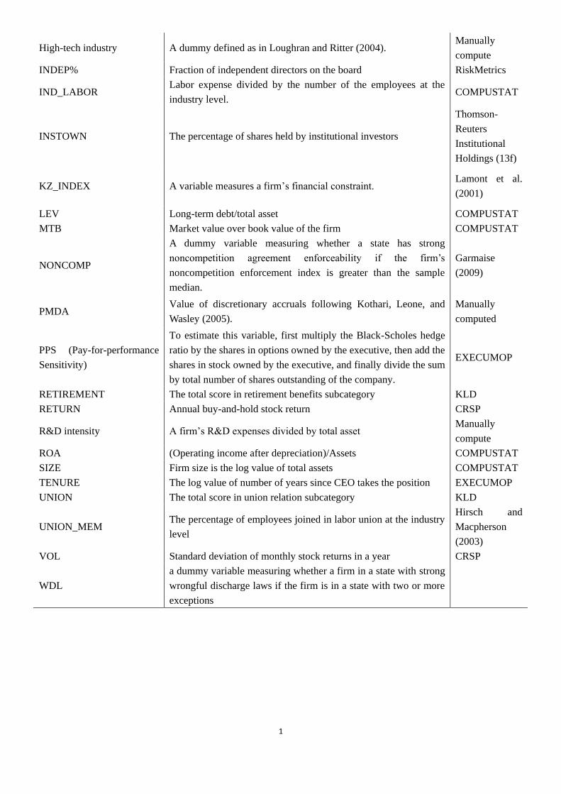
1

High-tech industry A dummy defined as in Loughran and Ritter (2004). Manually

compute

INDEP% Fraction of independent directors on the board RiskMetrics

IND_LABOR Labor expense divided by the number of the employees at the

industry level. COMPUSTAT

INSTOWN The percentage of shares held by institutional investors

Thomson-

Reuters

Institutional

Holdings (13f)

KZ_INDEX A variable measures a firm’s financial constraint. Lamont et al.

(2001)

LEV Long-term debt/total asset COMPUSTAT

MTB Market value over book value of the firm COMPUSTAT

NONCOMP

A dummy variable measuring whether a state has strong

noncompetition agreement enforceability if the firm’s

noncompetition enforcement index is greater than the sample

median.

Garmaise

(2009)

PMDA Value of discretionary accruals following Kothari, Leone, and

Wasley (2005).

Manually

computed

PPS (Pay-for-performance

Sensitivity)

To estimate this variable, first multiply the Black-Scholes hedge

ratio by the shares in options owned by the executive, then add the

shares in stock owned by the executive, and finally divide the sum

by total number of shares outstanding of the company.

EXECUMOP

RETIREMENT The total score in retirement benefits subcategory KLD

RETURN Annual buy-and-hold stock return CRSP

R&D intensity A firm’s R&D expenses divided by total asset Manually

compute

ROA (Operating income after depreciation)/Assets COMPUSTAT

SIZE Firm size is the log value of total assets COMPUSTAT

TENURE The log value of number of years since CEO takes the position EXECUMOP

UNION The total score in union relation subcategory KLD

UNION_MEM The percentage of employees joined in labor union at the industry

level

Hirsch and

Macpherson

(2003)

VOL Standard deviation of monthly stock returns in a year CRSP

WDL

a dummy variable measuring whether a firm in a state with strong

wrongful discharge laws if the firm is in a state with two or more

exceptions

1

Appendix II: Estimation of discretionary accruals

We use a modified version of the Jones model (Dechow, Sloan, and Sweeney, 1995) to

estimate discretionary accruals from regressions of total accruals on changes in sales and on

property, plant, and equipment within industries. To obtain discretionary accruals, we first run

a cross-sectional OLS regression within two-digit SIC code to estimate coefficients α1, α2, and

α3.

𝑇𝐴𝑖𝑡

𝐴𝑖𝑡−1= 𝛼1

1

𝐴𝑖𝑡−1+ 𝛼2

∆𝑅𝐸𝑉𝑖𝑡

𝐴𝑖𝑡−1+ 𝛼3

𝑃𝑃𝐸𝑖𝑡

𝐴𝑖𝑡−1+ 𝜀𝑖𝑡

where we indexes firms, t indexes time, 𝑇𝐴𝑖𝑡 is net income minus cash flow from

operations, ∆𝑅𝐸𝑉𝑖𝑡 is the changes in sales revenues, 𝐴𝑖𝑡−1 is the lagged value of firm’s total

assets. 𝑃𝑃𝐸𝑖𝑡 is the gross property, plant, and equipment, ∆𝐴𝑅𝑖𝑡 is the change in receivables.

We estimate the cross-sectional models separately for each combination of calendar year and

two-digit SIC code with a minimum of 15 observations. Then, we use the estimated �̂�1, �̂�2,

and �̂�3 to compute nondiscretionary accruals.

𝑁𝐷𝐴𝑖𝑡 ≡ �̂�1

1

𝐴𝑖𝑡−1+ �̂�2(

∆𝑅𝐸𝑉𝑖𝑡

𝐴𝑖𝑡−1−

∆𝐴𝑅𝑖𝑡

𝐴𝑖𝑡−1) + �̂�3

𝑃𝑃𝐸𝑖𝑡

𝐴𝑖𝑡−1

Therefore, the discretionary accruals is computed as

𝐷𝐴𝑖𝑡 ≡ 𝜀𝑖𝑡 =𝑇𝐴𝑖𝑡

𝐴𝑖𝑡−1− 𝑁𝐷𝐴𝑖𝑡

Since all the variables are scaled by total assets at the beginning of the period, the

magnitude of a firm's discretionary accruals is computed as a percentage of the assets of the

firm.

Following Kothari, Leone, and Wasley (2005), we augment the modified Jones model by

including ROAt-1 to avoid potential misspecification. The residuals from the annual cross-

sectional industry regression are treated as my performance-matched discretionary accruals.

1

We estimate the following regression:

𝑇𝐴𝑖𝑡

𝐴𝑖𝑡−1= 𝛼1

1

𝐴𝑖𝑡−1+ 𝛼2 (

∆𝑅𝐸𝑉𝑖𝑡

𝐴𝑖𝑡−1−

∆𝐴𝑅𝑖𝑡

𝐴𝑖𝑡−1) + 𝛼3

𝑃𝑃𝐸𝑖𝑡

𝐴𝑖𝑡−1+ 𝛼4

𝐼𝐵𝑋𝐼𝑖𝑡−1

𝐴𝑖𝑡−1+ 𝜀𝑖𝑡

where 𝐼𝐵𝑋𝐼𝑖𝑡−1 is income before extraordinary items at year t-1.

1

Appendix III: Estimation of discretionary accruals

Following existing literature (Roychowdhury, 2006 and Cohen, Dey, and Lys, 2008), sales

manipulations are negatively associated with current-period operating cash flows. We use

Roychowdhury (2006) model to estimate the normal value of operating cash flows:

𝐶𝐹𝑂𝑡

𝐴𝑡−1= 𝛼0 + 𝛼1 (

1

𝐴𝑡−1) + 𝛽1 (

𝑆𝑡

𝐴𝑡−1) + 𝛽2 (

∆𝑆𝑡

𝐴𝑡−1) + ε𝑡

where CFOt=cash flow from operation in year t, A=total assets, S=sales. For every firm-

year, abnormal cash flow from operations (AB_CFO) is the residual from the regression based

on year and two digit SIC industry code.

Abnormal production costs is another proxy for real activities manipulation. Following

Foychowdhury (2006), we estimate the following model for normal production costs:

𝑃𝑅𝑂𝐷𝑡

𝐴𝑡−1= 𝛼0 + 𝛼1 (

1

𝐴𝑡−1) + 𝛽1 (

𝑆𝑡

𝐴𝑡−1) + 𝛽2 (

∆𝑆𝑡

𝐴𝑡−1) + 𝛽3 (

∆𝑆𝑡−1

𝐴𝑡−1) + ε𝑡

Abnormal production cost (AB_PROD) is the residual from the model.

The third proxy for real activities manipulation is the abnormal discretionary expense.

Following Roychowdhury (2006), we estimate the normal level of discretionary expenses using

the following equations:

𝐷𝐼𝑆𝐸𝑋𝑃𝑡

𝐴𝑡−1= 𝛼0 + 𝛼1 (

1

𝐴𝑡−1) + 𝛽 (

𝑆𝑡

𝐴𝑡−1) + ε𝑡

where DISEXP is the discretionary expense in year t, computed as the sum of R&D,

Advertising, and SG&A expenses. For every firm-year, abnormal discretionary expenditure

(AB_EXP) is the residual from the model.

1

Table 1: Summary statistics

ABS_DA is absolute value of discretionary accruals computed from the modified Jone’s model

(Jones, 1991; Dechow, Sloan, and Sweeney, 1995). ERI is a firm’s total employee relation

strength score minus its total employee relation weakness score. The total employee relation

strength score is formed by adding the points a firm receives on criteria for employee relation

strength in the KLD database, and the total employ relation weakness score is formed by adding

the points the firm receives on criteria for employee relation weakness. SIZE is the log value of

total assets. BOARD is the number of board members sitting on the board. INDEP% is the

fraction of independent directors on the board. MTB is the market value over book value of the

firm. Following Wang (2013), FINANCE is measured by asset growth rate – ROA2/(1-ROA2),

ROA2 = (income before extraordinary items)/Assets. PPS (Pay-for-performance Sensitivity) is

measured by first multiplying the Black-Scholes hedge ratio by the shares in options owned by

the executive, then adding the shares in stock owned by the executive, and finally dividing the

sum by total number of shares outstanding of the company. LEV is measured by long-term

debt/total asset. INSTOWN is the percentage of shares held by institutional investors. ANALYST

is the number of analysts following the firm. CASH_VOL is the cash flow volatility following

Yu (2008). RETURN is the annual buy-and-hold stock return. VOL is the standard deviation of

monthly stock returns in a year.

(1) (2) (3) (4) (5)

VARIABLES N mean sd min max

ABS_DA 11,999 8.129 8.675 0.103 60.80

DA 11,999 -2.813 11.05 -48.51 40.77

ERI 11,999 -0.006 0.948 -2 3

BOARD 11,999 9.389 2.341 5 16

INDEP% 11,999 0.735 0.143 0.286 0.923

LEV 11,999 0.176 0.149 0 0.781

MTB 11,999 3.271 3.812 0.125 43.87

ROA 11,999 0.052 0.0910 -1.845 0.355

SIZE 11,999 7.848 1.407 2.876 10.65

FINANCE 11,999 -0.067 0.278 -0.738 2.115

CASH_VOL 11,999 0.072 0.09 0.006 1.020

PPS 11,999 18.06 42.08 0.0173 269.6

INSTOWN 11,999 0.758 0.190 0 1.147

ANALYST 11,999 6.143 7.097 0 28

RETURN 11,999 0.134 0.419 -0.765 2.171

VOL 11,999 0.103 0.0531 0.0302 0.360

1

Table 2: Correlation matrix

ABS_DA is Absolute value of discretionary accruals computed from the modified Jone’s model (Dechow, Sloan, and Sweeney, 1995). ABS_PMDA is the absolute value of

performance-matched discretionary accruals following Kothari, Leone, and Wasley (2005). ERI is a firm’s total employee relation strength score minus its total employee

relation weakness score. The total employee relation strength score is formed by adding the points a firm receives on criteria for employee relation strength in the KLD database,

and the total employ relation weakness score is formed by adding the points the firm receives on criteria for employee relation weakness. SIZE is the log value of total assets.

BOARD is the number of board members sitting on the board. INDEP% is the fraction of independent directors on the board. MTB is the market value over book value of the

firm. Following Wang (2013), FIN is measured by asset growth rate – ROA2/(1-ROA2), ROA2 = (income before extraordinary items)/Assets. PPS (Pay-for-performance

Sensitivity) is measured by first multiplying the Black-Scholes hedge ratio by the shares in options owned by the executive, then adding the shares in stock owned by the

executive, and finally dividing the sum by total number of shares outstanding of the company. LEV is measured by long-term debt/total asset. INSTOWN is the percentage of

shares held by institutional investors. ANALYST is the number of analysts following the firm. CASH_VOL is the cash flow volatility following Yu (2008). RETURN is the annual

buy-and-hold stock return. VOL is the standard deviation of monthly stock returns in a year.

ABS_DA ABS_PMDA EMP SIZE BOARD INDEP% MTB FIN PPS LEV ROA INSTOWN ANALYST CASH_VOL RETURN VOL

ABS_DA 1.00

ABS_PMDA 0.49 1.00

ERI 0.001 0.03 1.00

SIZE -0.08 -0.11 0.16 1.00

BOARD -0.03 -0.15 0.07 0.50 1.00

INDEP% -0.03 -0.01 0.00 0.07 0.05 1.00

MTB 0.00 0.09 0.07 0.24 0.04 -0.03 1.00

FINANCE 0.06 0.07 0.00 0.02 -0.02 -0.05 -0.13 1.00

PPS 0.01 0.02 -0.05 -0.21 -0.21 -0.22 -0.02 -0.03 1.00

LEV 0.05 -0.09 -0.05 0.09 0.20 0.08 0.05 0.11 -0.14 1.00

ROA -0.24 -0.22 0.07 0.22 0.01 -0.03 0.25 -0.13 0.05 -0.18 1.00

INSTOWN 0.00 0.09 -0.09 -0.15 -0.24 0.21 -0.04 0.05 -0.14 -0.01 0.01 1.00

ANALYST 0.02 0.05 -0.05 0.31 0.06 0.09 0.01 0.01 -0.09 -0.01 0.00 0.16 1.00

CASH_VOL 0.11 0.21 0.03 -0.04 -0.16 -0.14 0.19 0.15 0.03 -0.16 0.04 -0.03 0.01 1.00

RETURN 0.00 0.00 0.00 0.11 -0.03 -0.03 0.14 0.06 0.00 -0.05 0.13 0.00 0.01 0.13 1.00

VOL 0.15 0.22 -0.05 -0.33 -0.23 -0.07 -0.05 0.04 0.06 -0.03 -0.27 0.07 0.01 0.19 -0.01 1.00

1

Table 3: The effect of the Employee Treatment Index on earnings management in OLS

regression

This table reports the results of ordinary least squares regressions examining the effect of the

Employee Treatment Index on earnings management. The dependent variable is ABS_DA.

ABS_DA is the absolute value of discretionary accruals computed from the modified Jone’s

model (Dechow, Sloan, and Sweeney, 1995). ERI is a firm’s total employee relation strength

score minus its total employee relation weakness score. The total employee relation strength

score is formed by adding the points a firm receives on criteria for employee relation strength

in the KLD database, and the total employ relation weakness score is formed by adding the

points the firm receives on criteria for employee relation weakness. SIZE is the log value of

total assets. BOARD is the number of board members sitting on the board. INDEP% is the

fraction of independent directors on the board. MTB is the market value over book value of the

firm. Following Wang (2013), FINANCE is measured by asset growth rate – ROA2/(1-ROA2),

ROA2 = (income before extraordinary items)/Assets. PPS (Pay-for-performance Sensitivity) is

measured by first multiplying the Black-Scholes hedge ratio by the shares in options owned by

the executive, then adding the shares in stock owned by the executive, and finally dividing the

sum by total number of shares outstanding of the company. LEV is measured by long-term

debt/total asset. INSTOWN is the percentage of shares held by institutional investors. ANALYST

is the number of analysts following the firm. CASH_VOL is the cash flow volatility following

Yu (2008). RETURN is the annual buy-and-hold stock return. VOL is the standard deviation of

monthly stock returns in a year. Two-way clustered standard errors at the firm and year level

are used to calculate the t-statistics in parentheses, *** p<0.01, ** p<0.05, * p<0.1

(1) (2) (3)

All firms Firms with

positive DA

Firms with

negative DA

ERI 0.23** 0.0004 0.34***

(2.50) (0.00) (2.72)

SIZE -0.16* -0.33** -0.19*

(-1.87) (-2.36) (-1.73)

BOARD -0.08* 0.14* -0.13**

(-1.75) (1.75) (-2.47)

INDEP% -0.89 0.44 -0.98

(-1.31) (0.41) (-1.56)

MTB 0.16*** -0.04 0.20***

(4.55) (-0.76) (4.63)

FINANCE 1.41*** 3.32*** 1.30***

(2.90) (3.94) (2.70)

PPS 0.00 0.00 -0.00

(0.09) (0.57) (-0.04)

LEV -2.89*** 1.68 -3.20***

(-3.60) (1.22) (-3.73)

ROA -24.91*** 19.33*** -30.71***

(-5.68) (4.83) (-10.49)

INSTOWN -0.03 0.37 -0.20

1

(-0.06) (0.54) (-0.31)

ANALYST 0.04 -0.05 0.07***

(1.32) (-1.34) (2.68)

CASH_VOL 8.39*** 1.20 9.66***

(4.11) (0.48) (4.58)

RETURN 0.50 0.36 0.54

(1.56) (0.80) (1.64)

VOL 8.06** 15.88*** 3.69

(2.18) (3.34) (0.89)

Constant 12.76*** 6.87*** 12.57***

(7.62) (3.87) (6.56)

Industry fixed effect Yes Yes Yes

Year fixed effect Yes Yes Yes

Observations 11,999 4,222 7,777

R-squared 0.21 0.21 0.30

1

Table 4: Subcategories of the Employee Treatment Index and income-decreasing earnings

manipulation

This table reports the results of ordinary least squares regressions examining the effect of the

Employee Treatment Index on income-decreasing earnings management. The dependent

variable is ABS_DA. ABS_DA is absolute value of discretionary accruals computed from the

modified Jone’s model (Dechow, Sloan, and Sweeney, 1995). UNION is the total score in union

relation subcategory. RETIREMENT is the total score in retirement benefits subcategory.

HEALTH is the total score in health and safety subcategory. CASH_PROFIT is the total score

in cash profit-sharing program subcategory. EMP_INVOLVE is the total score in employee

involvement subcategory. SIZE is the log value of total assets. BOARD is the number of board

members sitting on the board. INDEP% is the fraction of independent directors on the board.

MTB is the market value over book value of the firm. Following Wang (2013), FINANCE is

measured by asset growth rate – ROA2/(1-ROA2), ROA2 = (income before extraordinary

items)/Assets. PPS (Pay-for-performance Sensitivity) is measured by first multiplying the

Black-Scholes hedge ratio by the shares in options owned by the executive, then adding the

shares in stock owned by the executive, and finally dividing the sum by total number of shares

outstanding of the company. LEV is measured by long-term debt/total asset. INSTOWN is the

percentage of shares held by institutional investors. ANALYST is the number of analysts

following the firm. CASH_VOL is the cash flow volatility following Yu (2008). RETURN is the

annual buy-and-hold stock return. VOL is the standard deviation of monthly stock returns in a

year. Two-way clustered standard errors at the firm and year level are used to calculate the t-

statistics in parentheses, *** p<0.01, ** p<0.05, * p<0.1

Firms with Negative DA

(1) (2) (3) (4) (5)

UNION 0.30

(0.50)

RETIREMENT 0.41

(1.48)

HEALTH 0.18

(0.85)

CASH_PROFIT 0.75**

(2.02)

EMP_INVOVLE 0.56

(1.49)

SIZE -0.19 -0.22* -0.13 -0.19* -0.20*

(-1.47) (-1.69) (-0.94) (-1.72) (-1.79)

BOARD -0.13** -0.14** -0.11* -0.13** -0.13**

(-2.11) (-2.18) (-1.81) (-2.43) (-2.39)

INDEP% -0.98 -0.86 -1.17 -1.05* -1.01

(-1.55) (-1.29) (-1.51) (-1.69) (-1.62)

MTB 0.21*** 0.22*** 0.21*** 0.20*** 0.20***

(4.30) (4.38) (4.40) (4.92) (4.78)

FINANCE 1.53*** 1.48*** 0.95* 1.30*** 1.30***

(2.95) (2.81) (1.69) (2.67) (2.66)

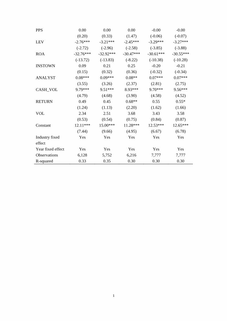
1

PPS 0.00 0.00 0.00 -0.00 -0.00

(0.20) (0.33) (1.47) (-0.06) (-0.07)

LEV -2.76*** -3.21*** -2.45*** -3.29*** -3.27***

(-2.72) (-2.96) (-2.58) (-3.85) (-3.88)

ROA -32.76*** -32.92*** -30.47*** -30.61*** -30.55***

(-13.72) (-13.83) (-8.22) (-10.38) (-10.28)

INSTOWN 0.09 0.21 0.25 -0.20 -0.21

(0.15) (0.32) (0.36) (-0.32) (-0.34)

ANALYST 0.08*** 0.09*** 0.08** 0.07*** 0.07***

(3.55) (3.26) (2.37) (2.81) (2.75)

CASH_VOL 9.79*** 9.51*** 8.93*** 9.70*** 9.56***

(4.79) (4.68) (3.90) (4.58) (4.52)

RETURN 0.49 0.45 0.68** 0.55 0.55*

(1.24) (1.13) (2.20) (1.62) (1.66)

VOL 2.34 2.51 3.68 3.43 3.58

(0.53) (0.54) (0.75) (0.84) (0.87)

Constant 12.11*** 15.00*** 11.28*** 12.53*** 12.65***

(7.44) (9.66) (4.95) (6.67) (6.78)

Industry fixed

effect

Yes Yes Yes Yes Yes

Year fixed effect Yes Yes Yes Yes Yes

Observations 6,128 5,752 6,216 7,777 7,777

R-squared 0.33 0.35 0.30 0.30 0.30

1

Table 5: Firm’s characteristics and the Employee Treatment Index

This table reports the results of ordinary least squares regressions examining the effect of the

Employee Treatment Index on earnings management. The dependent variable is ABS_DA.

ABS_DA is absolute value of discretionary accruals computed from the modified Jone’s model

(Dechow, Sloan, and Sweeney, 1995). ERI is a firm’s total employee relation strength score

minus its total employee relation weakness score. The total employee relation strength score is

formed by adding the points a firm receives on criteria for employee relation strength in the

KLD database, and the total employ relation weakness score is formed by adding the points the

firm receives on criteria for employee relation weakness. SIZE is the log value of total assets.

BOARD is the number of board members sitting on the board. INDEP% is the fraction of

independent directors on the board. MTB is the market value over book value of the firm.

Following Wang (2013), FINANCE is measured by asset growth rate – ROA2/(1-ROA2),

ROA2 = (income before extraordinary items)/Assets. PPS (Pay-for-performance Sensitivity) is

measured by first multiplying the Black-Scholes hedge ratio by the shares in options owned by

the executive, then adding the shares in stock owned by the executive, and finally dividing the

sum by total number of shares outstanding of the company. LEV is measured by long-term

debt/total asset. INSTOWN is the percentage of shares held by institutional investors. ANALYST

is the number of analysts following the firm. CASH_VOL is the cash flow volatility following

Yu (2008). RETURN is the annual buy-and-hold stock return. VOL is the standard deviation of

monthly stock returns in a year. Two-way clustered standard errors at the firm and year level

are used to calculate the t-statistics in parentheses, *** p<0.01, ** p<0.05, * p<0.1

All firms

R&D intensity High-tech industry Industry competition

High Low Yes No Low High

ERI 0.52*** -0.04 0.63*** 0.12 0.16 0.25**

(2.72) (-0.24) (3.24) (1.10) (1.05) (2.49)

SIZE 0.27 -0.24 0.24 -0.33*** -0.40*** 0.04

(1.49) (-1.32) (1.19) (-3.46) (-2.94) (0.38)

BOARD -0.17 -0.04 0.04 -0.05 -0.04 -0.10*

(-1.44) (-0.41) (0.28) (-1.09) (-0.66) (-1.75)

INDEP% 0.44 -0.25 0.46 -0.97 -0.71 -0.24

(0.29) (-0.19) (0.39) (-1.25) (-0.82) (-0.28)

MTB 0.22*** 0.05 0.36*** 0.11*** 0.16*** 0.15***

(2.59) (1.41) (3.49) (3.33) (2.95) (3.63)

FINANCE 3.52*** 0.50 3.04*** 1.12* 1.33 1.49***

(4.15) (0.75) (3.24) (1.85) (1.49) (3.33)

PPS 0.00 0.00 -0.00 0.00 -0.00 0.00

(0.47) (0.71) (-0.07) (0.15) (-1.02) (1.59)

LEV -3.88** -3.10*** -8.07*** -1.41* -3.67*** -2.12**

(-2.02) (-2.91) (-5.78) (-1.79) (-3.60) (-2.06)

ROA -28.03*** -23.68*** -32.59*** -20.10*** -21.59*** -27.37***

(-7.32) (-4.46) (-14.69) (-3.31) (-3.73) (-7.29)

INSTOWN 0.15 -2.38*** 1.87* -0.22 -0.41 0.45

(0.15) (-3.84) (1.75) (-0.43) (-0.74) (0.67)

1

ANALYST 0.01 0.04 0.02 0.04 0.01 0.06**

(0.38) (0.77) (0.94) (1.00) (0.18) (2.34)

CASH_VOL 4.37* 8.70*** 3.88 9.46*** 9.02*** 6.93***

(1.93) (2.59) (1.38) (4.00) (3.29) (2.92)

RETURN 0.54 0.72** 0.14 0.43 0.45 0.49

(0.86) (2.00) (0.29) (1.47) (1.24) (1.33)

VOL 12.10** 5.01 11.55*** 7.45* 7.33* 12.07***

(2.26) (1.30) (3.36) (1.95) (1.96) (3.25)

Constant 8.27*** 11.05*** 10.76 13.77*** 14.57*** 3.60**

(3.69) (3.91) (0.28) (7.20) (5.98) (2.40)

Industry fixed

effect

Yes Yes Yes Yes Yes Yes

Year fixed

effect

Yes Yes Yes Yes Yes Yes

Observations 3,148 3,810 2,160 9,839 6,172 5,827

R-squared 0.30 0.20 0.40 0.19 0.20 0.24

1

Table 6: The effect of the Employee Treatment Index on earnings management in OLS

regression controlling for firm-fixed effect

The dependent variable is ABS_DA. ABS_DA is the absolute value of discretionary accruals

computed from the modified Jone’s model (Dechow, Sloan, and Sweeney, 1995). ERI is a firm’s

total employee relation strength score minus its total employee relation weakness score. The

total employee relation strength score is formed by adding the points a firm receives on criteria

for employee relation strength in the KLD database, and the total employ relation weakness

score is formed by adding the points the firm receives on criteria for employee relation

weakness. SIZE is the log value of total assets. BOARD is the number of board members sitting

on the board. INDEP% is the fraction of independent directors on the board. MTB is the market

value over book value of the firm. Following Wang (2013), FINANCE is measured by asset

growth rate – ROA2/(1-ROA2), ROA2 = (income before extraordinary items)/Assets. PPS

(Pay-for-performance Sensitivity) is measured by first multiplying the Black-Scholes hedge

ratio by the shares in options owned by the executive, then adding the shares in stock owned

by the executive, and finally dividing the sum by total number of shares outstanding of the

company. LEV is measured by long-term debt/total asset. INSTOWN is the percentage of shares

held by institutional investors. ANALYST is the number of analysts following the firm.

CASH_VOL is the cash flow volatility following Yu (2008). RETURN is the annual buy-and-

hold stock return. VOL is the standard deviation of monthly stock returns in a year. Two-way

clustered standard errors at the firm and year level are used to calculate the t-statistics in

parentheses, *** p<0.01, ** p<0.05, * p<0.1

(1) (2) (3)

All firms Firms with

Positive DA

Firms with

Negative DA

ERI 0.21* 0.004 0.35**

(1.86) (0.02) (2.48)

SIZE 1.20*** 0.37 1.42***

(3.95) (0.59) (4.07)

BOARD 0.02 0.08 0.05

(0.34) (0.49) (0.47)

INDEP% -1.66 -3.70 0.43

(-1.33) (-1.54) (0.31)

MTB 0.07 0.00 0.05

(1.48) (0.04) (1.06)

FINANCE 2.67*** 4.72*** 2.60***

(5.54) (4.98) (3.38)

PPS 0.00 0.01 -0.00

(0.72) (1.22) (-0.47)

LEV -3.34** -3.22 -1.20

(-2.45) (-1.21) (-0.77)

ROA -34.00*** 25.51*** -42.79***

(-7.08) (3.47) (-17.86)

INSTOWN -1.81 4.14 -2.96**

(-1.58) (1.41) (-2.09)

1

ANALYST -0.00 -0.08* 0.02

(-0.05) (-1.94) (0.94)

CASH_VOL 9.03*** 2.12 12.86***

(2.82) (0.39) (4.52)

RETURN 0.18 0.01 0.12

(0.60) (0.01) (0.38)

VOL 3.29 15.55** -1.02

(0.92) (2.29) (-0.34)

Constant 2.18 0.80 -0.13

(0.73) (0.13) (-0.04)

Firm fixed effect Yes Yes Yes

Year fixed effect Yes Yes Yes

Observations 11,999 4,222 7,777

R-squared 0.39 0.19 0.30

1

Table 7: The effect of changes in the Employee Treatment Index on changes in the signed

discretionary accruals

The dependent variable is change in signed discretionary accruals between year t-1 and year t.

All independent variables are measured as changes between year t-1 and year t. DA is the

discretionary accruals computed from the modified Jone’s model (Dechow, Sloan, and Sweeney,

1995). ERI is a firm’s total employee relation strength score minus its total employee relation

weakness score. The total employee relation strength score is formed by adding the points a

firm receives on criteria for employee relation strength in the KLD database, and the total

employ relation weakness score is formed by adding the points the firm receives on criteria for

employee relation weakness. SIZE is the log value of total assets. BOARD is the number of

board members sitting on the board. INDEP% is the fraction of independent directors on the

board. MTB is the market value over book value of the firm. Following Wang (2013), FINANCE

is measured by asset growth rate – ROA2/(1-ROA2), ROA2 = (income before extraordinary

items)/Assets. PPS (Pay-for-performance Sensitivity) is measured by first multiplying the

Black-Scholes hedge ratio by the shares in options owned by the executive, then adding the

shares in stock owned by the executive, and finally dividing the sum by total number of shares

outstanding of the company. LEV is measured by long-term debt/total asset. INSTOWN is the

percentage of shares held by institutional investors. ANALYST is the number of analysts

following the firm. CASH_VOL is the cash flow volatility following Yu (2008). RETURN is the

annual buy-and-hold stock return. VOL is the standard deviation of monthly stock returns in a

year. Two-way clustered standard errors at the firm and year level are used to calculate the t-

statistics in parentheses, *** p<0.01, ** p<0.05, * p<0.1

All firms Firms with

Positive DA

Firms with

Negative DA

ΔERI -0.38* -0.02 -0.47***

(-1.81) (-0.06) (-2.87)

ΔSIZE -0.49 -0.59 -1.50*

(-0.58) (-0.50) (-1.93)

ΔBOARD -0.05 0.34 -0.32*

(-0.30) (1.19) (-1.76)

ΔINDEP% -2.77 -3.44 -1.14

(-1.61) (-1.22) (-0.44)

ΔMTB 0.04 0.07 0.03

(0.36) (0.34) (0.40)

ΔFINANCE 0.77 3.54*** -1.34*

(0.83) (4.35) (-1.65)

ΔPPS -0.01 -0.01 -0.00

(-0.50) (-0.50) (-0.33)

ΔLEV -3.13 1.17 -5.23**

(-1.20) (0.33) (-2.02)

ΔROA 52.98*** 61.09*** 47.33***

(12.31) (12.18) (14.62)

ΔINSTOWN 2.21 3.64 4.04*

(1.10) (1.13) (1.85)

1

ΔANALYST -0.05 -0.06 -0.04

(-1.06) (-1.08) (-1.09)

ΔCASH_VOL -19.98*** -10.80 -20.62**

(-2.78) (-1.05) (-2.36)

ΔRETURN -0.12 0.02 0.28

(-0.22) (0.03) (0.64)

ΔVOL 3.16 7.08 0.36

(0.56) (0.78) (0.05)

Constant 0.74 13.76** -12.82***

(0.19) (2.53) (-4.22)

Industry fixed effect Yes Yes Yes

Year fixed effect Yes Yes Yes

Observations 9,911 3,457 6,454

R-squared 0.14 0.24 0.19

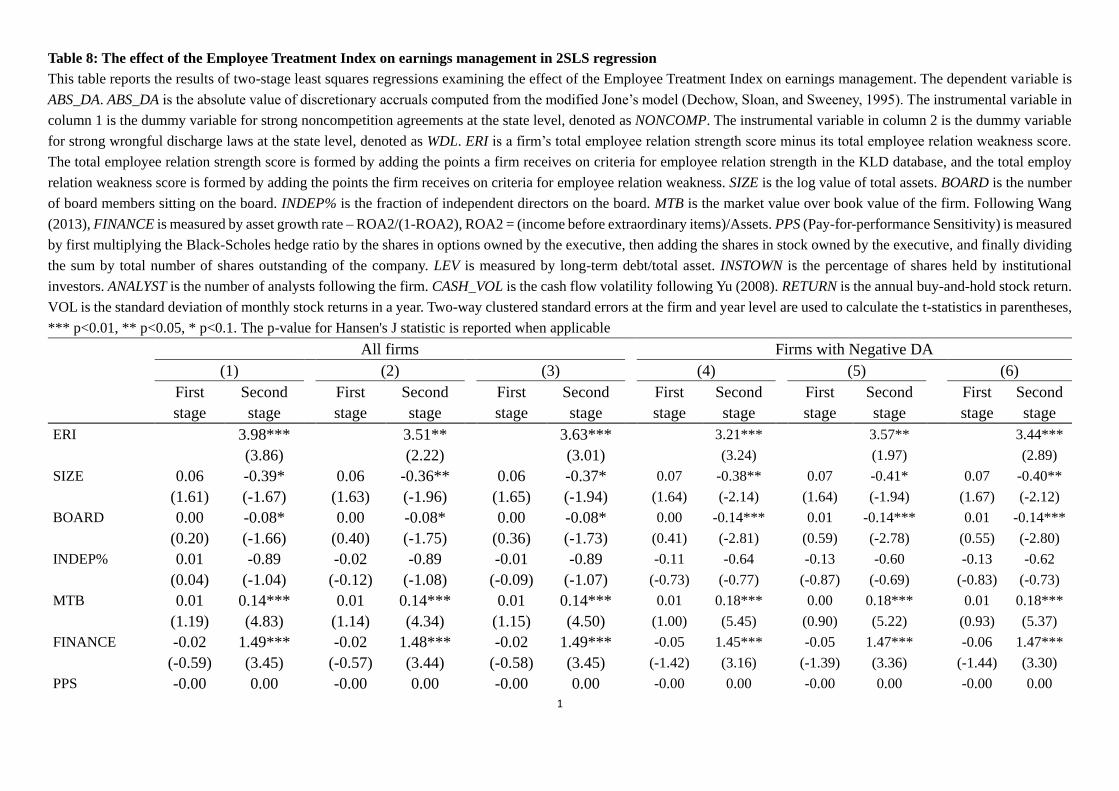
1

Table 8: The effect of the Employee Treatment Index on earnings management in 2SLS regression

This table reports the results of two-stage least squares regressions examining the effect of the Employee Treatment Index on earnings management. The dependent variable is

ABS_DA. ABS_DA is the absolute value of discretionary accruals computed from the modified Jone’s model (Dechow, Sloan, and Sweeney, 1995). The instrumental variable in

column 1 is the dummy variable for strong noncompetition agreements at the state level, denoted as NONCOMP. The instrumental variable in column 2 is the dummy variable

for strong wrongful discharge laws at the state level, denoted as WDL. ERI is a firm’s total employee relation strength score minus its total employee relation weakness score.

The total employee relation strength score is formed by adding the points a firm receives on criteria for employee relation strength in the KLD database, and the total employ

relation weakness score is formed by adding the points the firm receives on criteria for employee relation weakness. SIZE is the log value of total assets. BOARD is the number

of board members sitting on the board. INDEP% is the fraction of independent directors on the board. MTB is the market value over book value of the firm. Following Wang

(2013), FINANCE is measured by asset growth rate – ROA2/(1-ROA2), ROA2 = (income before extraordinary items)/Assets. PPS (Pay-for-performance Sensitivity) is measured

by first multiplying the Black-Scholes hedge ratio by the shares in options owned by the executive, then adding the shares in stock owned by the executive, and finally dividing

the sum by total number of shares outstanding of the company. LEV is measured by long-term debt/total asset. INSTOWN is the percentage of shares held by institutional

investors. ANALYST is the number of analysts following the firm. CASH_VOL is the cash flow volatility following Yu (2008). RETURN is the annual buy-and-hold stock return.

VOL is the standard deviation of monthly stock returns in a year. Two-way clustered standard errors at the firm and year level are used to calculate the t-statistics in parentheses,

*** p<0.01, ** p<0.05, * p<0.1. The p-value for Hansen's J statistic is reported when applicable

All firms Firms with Negative DA

(1) (2) (3) (4) (5) (6)

First

stage

Second

stage

First

stage

Second

stage

First

stage

Second

stage

First

stage

Second

stage

First

stage

Second

stage

First

stage

Second

stage

ERI 3.98*** 3.51** 3.63*** 3.21*** 3.57** 3.44***

(3.86) (2.22) (3.01) (3.24) (1.97) (2.89)

SIZE 0.06 -0.39* 0.06 -0.36** 0.06 -0.37* 0.07 -0.38** 0.07 -0.41* 0.07 -0.40**

(1.61) (-1.67) (1.63) (-1.96) (1.65) (-1.94) (1.64) (-2.14) (1.64) (-1.94) (1.67) (-2.12)

BOARD 0.00 -0.08* 0.00 -0.08* 0.00 -0.08* 0.00 -0.14*** 0.01 -0.14*** 0.01 -0.14***

(0.20) (-1.66) (0.40) (-1.75) (0.36) (-1.73) (0.41) (-2.81) (0.59) (-2.78) (0.55) (-2.80)

INDEP% 0.01 -0.89 -0.02 -0.89 -0.01 -0.89 -0.11 -0.64 -0.13 -0.60 -0.13 -0.62

(0.04) (-1.04) (-0.12) (-1.08) (-0.09) (-1.07) (-0.73) (-0.77) (-0.87) (-0.69) (-0.83) (-0.73)

MTB 0.01 0.14*** 0.01 0.14*** 0.01 0.14*** 0.01 0.18*** 0.00 0.18*** 0.01 0.18***

(1.19) (4.83) (1.14) (4.34) (1.15) (4.50) (1.00) (5.45) (0.90) (5.22) (0.93) (5.37)

FINANCE -0.02 1.49*** -0.02 1.48*** -0.02 1.49*** -0.05 1.45*** -0.05 1.47*** -0.06 1.47***

(-0.59) (3.45) (-0.57) (3.44) (-0.58) (3.45) (-1.42) (3.16) (-1.39) (3.36) (-1.44) (3.30)

PPS -0.00 0.00 -0.00 0.00 -0.00 0.00 -0.00 0.00 -0.00 0.00 -0.00 0.00

1

(-1.70) (0.97) (-1.71) (0.91) (-1.73) (0.94) (-1.56) (0.59) (-1.58) (0.57) (-1.58) (0.59)

LEV -0.37*** -1.47* -0.36*** -1.65 -0.36*** -1.61* -0.42*** -1.99* -0.40*** -1.84 -0.40*** -1.90*

(-3.10) (-1.69) (-3.04) (-1.62) (-3.03) (-1.71) (-3.05) (-1.81) (-2.98) (-1.55) (-2.96) (-1.76)

ROA 0.40** -26.41*** 0.40** -26.22*** 0.40** -26.26*** 0.41** -31.88*** 0.41** -32.03*** 0.41** -31.97***

(2.23) (-6.52) (2.25) (-6.52) (2.27) (-6.54) (2.47) (-11.44) (2.45) (-11.63) (2.50) (-11.69)

INSTOWN -0.18 0.58 -0.16 0.50 -0.17 0.52 -0.16 0.24 -0.16 0.30 -0.16 0.28

(-1.66) (1.03) (-1.59) (0.77) (-1.67) (0.84) (-1.52) (0.33) (-1.49) (0.35) (-1.55) (0.35)

ANALYST 0.01 0.01 0.01 0.01 0.01 0.01 0.01 0.05* 0.01 0.05 0.01 0.05*

(1.34) (0.37) (1.23) (0.40) (1.25) (0.40) (1.42) (1.89) (1.35) (1.54) (1.37) (1.73)

CASH_VOL 0.09 8.06*** 0.06 8.10*** 0.07 8.09*** 0.19 9.15*** 0.16 9.09*** 0.17 9.11***

(0.54) (4.31) (0.38) (4.34) (0.41) (4.34) (0.95) (4.69) (0.82) (4.61) (0.86) (4.66)

RETURN -0.06* 0.71** -0.06* 0.68** -0.06* 0.69** -0.06 0.71** -0.06 0.73** -0.06 0.73**

(-2.03) (2.27) (-2.02) (2.12) (-2.02) (2.18) (-1.71) (2.43) (-1.65) (2.23) (-1.67) (2.34)

VOL -0.09 8.43** -0.12 8.38** -0.11 8.39** -0.08 3.93 -0.10 3.96 -0.09 3.95

(-0.30) (2.22) (-0.42) (2.23) (-0.38) (2.23) (-0.22) (0.90) (-0.27) (0.89) (-0.25) (0.90)

NONCOMP -0.53*** -0.43** -0.62*** -0.53***

(-3.07) (-2.50) (-4.24) (-3.55)

WDL 0.12*** 0.11*** 0.11** 0.10**

(3.19) (3.00) (2.71) (2.51)

Industry fixed

effect

Yes Yes Yes Yes Yes Yes Yes Yes Yes Yes Yes Yes

Year fixed

effect

Yes Yes Yes Yes Yes Yes Yes Yes Yes Yes Yes Yes

F statistic 9.44 10.19 9.18 17.96 7.33 12.65

Hansen J

statistic (P-

value)

0.7988 0.8636

Observations 11,999 11,999 11,999 11,999 11,999 11,999 7,777 7,777 7,777 7,777 7,777 7,777

R-squared 0.03 0.07 0.03 0.03 0.03 0.04 0.02 0.08 0.04 0.05 0.04 0.06

1

Table 9: Performance-matched discretionary accruals and the Employee Treatment Index

This table reports the results of ordinary least squares regressions examining the effect of the

Employee Treatment Index on earnings management. The dependent variable is ABS_PMDA.

ABS_PMDA is the absolute value of performance-matched discretionary accruals following

Kothari, Leone, and Wasley (2005). ERI is a firm’s total employee relation strength score minus

its total employee relation weakness score. The total employee relation strength score is formed

by adding the points a firm receives on criteria for employee relation strength in the KLD

database, and the total employ relation weakness score is formed by adding the points the firm

receives on criteria for employee relation weakness. SIZE is the log value of total assets.

BOARD is the number of board members sitting on the board. INDEP% is the fraction of

independent directors on the board. MTB is the market value over book value of the firm.

Following Wang (2013), FINANCE is measured by asset growth rate – ROA2/(1-ROA2),

ROA2 = (income before extraordinary items)/Assets. PPS (Pay-for-performance Sensitivity) is

measured by first multiplying the Black-Scholes hedge ratio by the shares in options owned by

the executive, then adding the shares in stock owned by the executive, and finally dividing the

sum by total number of shares outstanding of the company. LEV is measured by long-term

debt/total asset. INSTOWN is the percentage of shares held by institutional investors. ANALYST

is the number of analysts following the firm. CASH_VOL is the cash flow volatility following

Yu (2008). RETURN is the annual buy-and-hold stock return. VOL is the standard deviation of

monthly stock returns in a year. Two-way clustered standard errors at the firm and year level

are used to calculate the t-statistics in parentheses, *** p<0.01, ** p<0.05, * p<0.1

All firms Firms with

Positive DA

Firms with

Negative DA

ERI 0.27*** 0.04 0.32***

(3.72) (0.43) (2.77)

SIZE -0.10 -0.37*** -0.09

(-1.22) (-3.92) (-0.94)

BOARD -0.09** 0.09* -0.12***

(-2.11) (1.66) (-2.80)

INDEP% -0.15 0.85 -0.42

(-0.32) (1.19) (-0.74)

MTB 0.19*** 0.01 0.26***

(5.71) (0.23) (5.49)

FINANCE 0.72* 2.04*** 0.64

(1.77) (3.23) (1.44)

PPS 0.00 -0.00 0.00

(0.45) (-0.62) (0.93)

LEV -3.73*** 0.81 -4.83***

(-8.36) (1.08) (-9.68)

ROA -15.28*** 12.41*** -19.67***

(-4.74) (6.44) (-8.44)

INSTOWN 0.75** -0.34 1.33***

(2.09) (-0.93) (2.59)

ANALYST 0.03* -0.05*** 0.05***

1

(1.78) (-2.65) (2.70)

CASH_VOL 8.18*** 5.26** 9.54***

(4.49) (2.43) (5.43)

RETURN 0.03 0.31 -0.12

(0.12) (1.00) (-0.33)

VOL 12.58*** 14.52*** 12.39***

(5.78) (5.77) (4.38)

Constant 4.17*** 0.90 4.68***

(4.43) (0.76) (4.29)

Industry fixed effect Yes Yes Yes

Year fixed effect Yes Yes Yes

Observations 11,948 4,152 7,796

R-squared 0.19 0.17 0.26

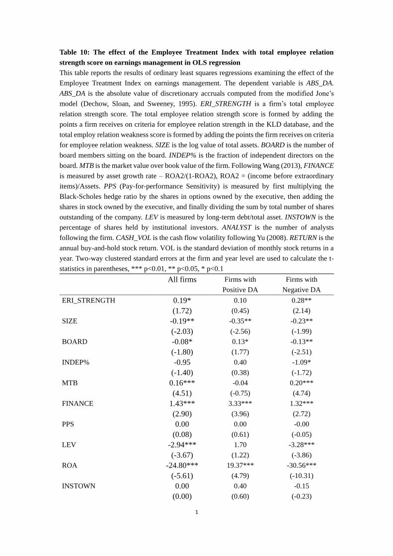
1

Table 10: The effect of the Employee Treatment Index with total employee relation

strength score on earnings management in OLS regression

This table reports the results of ordinary least squares regressions examining the effect of the

Employee Treatment Index on earnings management. The dependent variable is ABS_DA.

ABS_DA is the absolute value of discretionary accruals computed from the modified Jone’s

model (Dechow, Sloan, and Sweeney, 1995). ERI_STRENGTH is a firm’s total employee

relation strength score. The total employee relation strength score is formed by adding the

points a firm receives on criteria for employee relation strength in the KLD database, and the

total employ relation weakness score is formed by adding the points the firm receives on criteria

for employee relation weakness. SIZE is the log value of total assets. BOARD is the number of

board members sitting on the board. INDEP% is the fraction of independent directors on the

board. MTB is the market value over book value of the firm. Following Wang (2013), FINANCE

is measured by asset growth rate – ROA2/(1-ROA2), ROA2 = (income before extraordinary

items)/Assets. PPS (Pay-for-performance Sensitivity) is measured by first multiplying the

Black-Scholes hedge ratio by the shares in options owned by the executive, then adding the

shares in stock owned by the executive, and finally dividing the sum by total number of shares

outstanding of the company. LEV is measured by long-term debt/total asset. INSTOWN is the

percentage of shares held by institutional investors. ANALYST is the number of analysts

following the firm. CASH_VOL is the cash flow volatility following Yu (2008). RETURN is the

annual buy-and-hold stock return. VOL is the standard deviation of monthly stock returns in a

year. Two-way clustered standard errors at the firm and year level are used to calculate the t-

statistics in parentheses, *** p<0.01, ** p<0.05, * p<0.1

All firms Firms with

Positive DA

Firms with

Negative DA

ERI_STRENGTH 0.19* 0.10 0.28**

(1.72) (0.45) (2.14)

SIZE -0.19** -0.35** -0.23**

(-2.03) (-2.56) (-1.99)

BOARD -0.08* 0.13* -0.13**

(-1.80) (1.77) (-2.51)

INDEP% -0.95 0.40 -1.09*

(-1.40) (0.38) (-1.72)

MTB 0.16*** -0.04 0.20***

(4.51) (-0.75) (4.74)

FINANCE 1.43*** 3.33*** 1.32***

(2.90) (3.96) (2.72)

PPS 0.00 0.00 -0.00

(0.08) (0.61) (-0.05)

LEV -2.94*** 1.70 -3.28***

(-3.67) (1.22) (-3.86)

ROA -24.80*** 19.37*** -30.56***

(-5.61) (4.79) (-10.31)

INSTOWN 0.00 0.40 -0.15

(0.00) (0.60) (-0.23)

1

ANALYST 0.04 -0.05 0.07***

(1.32) (-1.34) (2.72)

CASH_VOL 8.37*** 1.20 9.64***

(4.08) (0.48) (4.56)

RETURN 0.51 0.37 0.56*

(1.60) (0.83) (1.68)

VOL 7.91** 15.81*** 3.45

(2.13) (3.38) (0.83)

Constant 12.96*** 6.98*** 12.85***

(7.72) (3.88) (6.71)

Year fixed effect Yes Yes Yes

Firm-fixed effect Yes Yes Yes

Observations 11,999 4,222 7,777

R-squared 0.21 0.21 0.30

1

Table 11: Test of the difference in earnings management between firms in Fortune's "100 Best Companies to Work For" and matching firms using

propensity score matching.

This table presents the test of the difference in earnings management between firms in Fortune magazine’s list of "100 Best Companies to Work For" and

matching firms in Compustat. The sample includes all publicly traded firms that are in Fortune's "100 Best Companies to Work For" from 1998 to 2008. The

dependent variable is ABS_DA. We match each firm in Fortune's list with a firm that is in Compustat but not in Fortune’s list using the nearest neighborhood, a

Gaussian kernel, and local linear regression matching approaches. The variables we use in matching are market-to-book ratio, log of sales, ratio of fixed assets

to total assets, return on assets, ratio of R&D expenditures to sales, ratio of SGA expenses to sales, dividend-paying dummy, ratio of sales to total assets, pension

and retirement expenses per worker, firm age, board size, and independent director%. Robust Abadie-Imbens standard errors are used to calculate the t-values

in parentheses. 95% confidence intervals are in brackets.

All firms Firms with Positive DA Firms with Negative DA

Propensity-score

Matching

Nearest-neighbor

matching

Propensity-score

Matching

Nearest-neighbor

matching

Propensity-score

Matching

Nearest-

neighbor

matching

2.65*** 3.24*** 6.73*** 6.32** 1.70** 1.88*

(2.67) (2.98) (6.93) (2.24) (2.29) (1.96)

[0.703, 4.605] [1.11, 5.366] [1.182, 10.321] [0.790, 11.847] [0.245, 3.153] [-0.096, 3.847]

1

Table 12: The effect of the Employee Treatment Index on earnings management in OLS regression controlling for substitution effect of real activities manipulation

The dependent variable is ABS_DA. ABS_DA is the absolute value of discretionary accruals computed from the modified Jone’s model (Dechow, Sloan, and Sweeney, 1995).

ERI is a firm’s total employee relation strength score minus its total employee relation weakness score. The total employee relation strength score is formed by adding the points

a firm receives on criteria for employee relation strength in the KLD database, and the total employ relation weakness score is formed by adding the points the firm receives on

criteria for employee relation weakness. AB_CFO is abnormal levels of operating cash flow. AB_PROD is abnormal production cost. AB_EXP is abnormal discretionary

expenses. COMBINED_RAM is a combined measure of real activities manipulation. SIZE is the log value of total assets. BOARD is the number of board members sitting on the

board. INDEP% is the fraction of independent directors on the board. MTB is the market value over book value of the firm. Following Wang (2013), FINANCE is measured by

asset growth rate – ROA2/(1-ROA2), ROA2 = (income before extraordinary items)/Assets. PPS (Pay-for-performance Sensitivity) is measured by first multiplying the Black-

Scholes hedge ratio by the shares in options owned by the executive, then adding the shares in stock owned by the executive, and finally dividing the sum by total number of

shares outstanding of the company. LEV is measured by long-term debt/total asset. INSTOWN is the percentage of shares held by institutional investors. ANALYST is the number

of analysts following the firm. CASH_VOL is the cash flow volatility following Yu (2008). RETURN is the annual buy-and-hold stock return. VOL is the standard deviation of

monthly stock returns in a year. Two-way clustered standard errors at the firm and year level are used to calculate the t-statistics in parentheses, *** p<0.01, ** p<0.05, * p<0.1

(1) (2) (3) (4)

All firms Firms with

Positive DA

Firms with

Negative

DA

All firms Firms with

Positive

DA

Firms with

Negative

DA

All firms Firms with

Positive

DA

Firms with

Negative

DA

All firms Firms with

Positive

DA

Firms with

Negative

DA

ERI 0.15* 0.02 0.21* 0.19** 0.07 0.28** 0.23** 0.0002 0.33*** 0.17* 0.07 0.24**

(1.69) (0.12) (1.86) (2.21) (0.45) (2.32) (2.50) (0.00) (2.69) (1.92) (0.41) (1.98)

AB_CFO 0.17*** -0.09** 0.32***

(6.26) (-2.53) (16.03)

AB_PROD -0.03*** 0.04*** -0.06***

(-3.65) (3.48) (-5.87)

AB_EXP 0.02 -0.003 0.03**

(1.11) (-0.13) (2.08)

COMBINED_RAM 0.04*** -0.03*** 0.07***

(6.29) (-3.31) (11.72)

SIZE -0.37*** -0.21 -0.52*** -0.17** -0.33** -0.21** -0.15* -0.33** -0.18 -0.20** -0.31** -0.25**

(-4.57) (-1.39) (-5.19) (-2.04) (-2.43) (-2.04) (-1.77) (-2.39) (-1.59) (-2.41) (-2.23) (-2.44)

BOARD -0.00 0.11 0.02 -0.06 0.14* -0.08 -0.08* 0.14* -0.13** -0.03 0.14* -0.03

(-0.02) (1.35) (0.46) (-1.27) (1.72) (-1.54) (-1.73) (1.73) (-2.39) (-0.78) (1.65) (-0.61)

INDEP% -0.48 0.34 0.08 -0.89 0.53 -0.90 -0.85 0.43 -0.95 -0.71 0.38 -0.57

1

(-0.72) (0.31) (0.13) (-1.26) (0.48) (-1.40) (-1.26) (0.41) (-1.50) (-1.02) (0.35) (-0.88)

MTB 0.12*** -0.04 0.12*** 0.13*** -0.02 0.14*** 0.15*** -0.04 0.19*** 0.11*** -0.02 0.10***

(3.80) (-0.70) (3.20) (3.62) (-0.38) (3.90) (4.38) (-0.75) (4.53) (3.41) (-0.43) (2.90)

FIN 1.58*** 3.36*** 1.50*** 1.65*** 3.29*** 1.61*** 1.37*** 3.32*** 1.19** 1.62*** 3.37*** 1.45***

(3.72) (3.94) (3.49) (3.42) (3.81) (3.32) (2.77) (3.93) (2.51) (3.44) (3.89) (3.18)

PPS 0.00 0.00 0.00 0.00 0.00 0.00 0.00 0.00 -0.00 0.00 0.00 0.00

(0.54) (0.35) (0.41) (0.18) (0.55) (0.03) (0.06) (0.57) (-0.10) (0.20) (0.50) (0.01)

LEV -2.09*** 1.71 -1.51* -2.63*** 1.46 -2.60*** -2.85*** 1.68 -3.11*** -2.27*** 1.45 -1.89**

(-2.71) (1.25) (-1.84) (-3.15) (1.02) (-3.03) (-3.48) (1.21) (-3.63) (-2.73) (1.03) (-2.28)

ROA -29.54*** 24.99*** -39.82*** -25.67*** 22.95*** -32.29*** -24.90*** 19.33*** -30.67*** -26.92*** 23.91*** -34.51***

(-7.57) (4.63) (-22.06) (-5.83) (5.48) (-11.69) (-5.64) (4.82) (-10.35) (-6.26) (5.27) (-14.27)

INSTOWN -0.29 0.35 -0.68 -0.09 0.04 -0.26 -0.05 0.37 -0.21 -0.18 0.14 -0.40

(-0.66) (0.49) (-1.39) (-0.18) (0.06) (-0.43) (-0.09) (0.55) (-0.32) (-0.39) (0.21) (-0.66)

ANALYST 0.03 -0.06 0.06** 0.04 -0.05 0.07*** 0.04 -0.05 0.07*** 0.03 -0.05 0.06**

(1.05) (-1.37) (2.23) (1.28) (-1.37) (2.87) (1.32) (-1.35) (2.66) (1.16) (-1.31) (2.46)

CASH_VOL 7.06*** 1.20 6.51*** 7.72*** 1.44 8.54*** 8.33*** 1.22 9.61*** 7.15*** 1.46 7.55***

(3.92) (0.47) (3.80) (3.82) (0.53) (4.19) (4.08) (0.49) (4.50) (3.68) (0.54) (3.79)

RETURN 0.47* 0.33 0.40 0.50 0.20 0.54 0.49 0.37 0.53 0.48 0.23 0.48

(1.68) (0.69) (1.43) (1.60) (0.47) (1.62) (1.54) (0.82) (1.59) (1.55) (0.53) (1.46)

VOL 7.27** 15.62*** 1.55 7.96** 16.71*** 3.19 8.04** 15.88*** 3.61 7.65** 16.46*** 2.41

(2.03) (3.17) (0.41) (2.32) (3.62) (0.85) (2.17) (3.35) (0.89) (2.24) (3.54) (0.68)

Constant 14.34*** 5.85*** 14.85*** 13.18*** 6.39*** 12.74*** 12.66*** 6.89*** 12.40*** 13.41*** 6.38*** 12.68***

(8.78) (3.16) (8.08) (7.92) (3.52) (6.78) (7.59) (3.93) (6.41) (8.34) (3.58) (6.92)

Industry fixed effect Yes Yes Yes Yes Yes Yes Yes Yes Yes Yes Yes Yes

Year fixed effect Yes Yes Yes Yes Yes Yes Yes Yes Yes Yes Yes Yes

Observations 11,948 4,210 7,738 11,707 4,121 7,586 11,999 4,222 7,777 11,707 4,121 7,586

R-squared 0.23 0.21 0.38 0.21 0.21 0.31 0.21 0.21 0.30 0.22 0.21 0.33

1

Table 13: The effect of the Employee Treatment Index on earnings management in OLS regression excluding non-articulation events

This table reports the results of ordinary least squares regressions examining the effect of the Employee Treatment Index on earnings management. The

dependent variable is ABS_DA. ABS_DA is the absolute value of discretionary accruals computed from the modified Jone’s model (Dechow, Sloan, and Sweeney,

1995). ERI is a firm’s total employee relation strength score minus its total employee relation weakness score. The total employee relation strength score is

formed by adding the points a firm receives on criteria for employee relation strength in the KLD database, and the total employ relation weakness score is

formed by adding the points the firm receives on criteria for employee relation weakness. SIZE is the log value of total assets. BOARD is the number of board

members sitting on the board. INDEP% is the fraction of independent directors on the board. MTB is the market value over book value of the firm. Following

Wang (2013), FINANCE is measured by asset growth rate – ROA2/(1-ROA2), ROA2 = (income before extraordinary items)/Assets. PPS (Pay-for-performance

Sensitivity) is measured by first multiplying the Black-Scholes hedge ratio by the shares in options owned by the executive, then adding the shares in stock

owned by the executive, and finally dividing the sum by total number of shares outstanding of the company. LEV is measured by long-term debt/total asset.

INSTOWN is the percentage of shares held by institutional investors. ANALYST is the number of analysts following the firm. CASH_VOL is the cash flow

volatility following Yu (2008). RETURN is the annual buy-and-hold stock return. VOL is the standard deviation of monthly stock returns in a year. Two-way

clustered standard errors at the firm and year level are used to calculate the t-statistics in parentheses, *** p<0.01, ** p<0.05, * p<0.1

Excluding M&A Excluding divestitures Excluding foreign

currency translations

All firms Firms with

Positive

DA

Firms with

Negative DA

All firms Firms with

Positive DA

Firms with

Negative

DA

All firms Firms

with

Positive

DA

Firms with

Negative

DA

ERI 0.23** -0.04 0.36*** 0.23** -0.08 0.36*** 0.25*** 0.02 0.36***

(2.54) (-0.30) (2.88) (2.23) (-0.51) (2.60) (2.64) (0.10) (2.73)

SIZE -0.16* -0.33** -0.19 -0.17* -0.37** -0.19 -0.20** -0.45*** -0.18

(-1.70) (-2.17) (-1.60) (-1.75) (-2.37) (-1.60) (-2.17) (-2.84) (-1.62)

BOARD -0.08 0.12 -0.13** -0.07 0.14 -0.12** -0.10** 0.13 -0.16***

(-1.62) (1.64) (-2.42) (-1.39) (1.54) (-2.23) (-2.31) (1.40) (-3.06)

INDEP% -0.70 0.23 -0.63 -1.07 -0.00 -1.15 -1.06 0.24 -1.08

1

(-1.03) (0.22) (-1.02) (-1.47) (-0.00) (-1.58) (-1.43) (0.20) (-1.35)

MTB 0.15*** -0.04 0.19*** 0.16*** -0.04 0.19*** 0.16*** -0.04 0.20***

(4.34) (-0.75) (4.66) (4.44) (-0.90) (4.40) (4.07) (-0.75) (4.93)

FINANCE 1.43*** 3.33*** 1.34*** 1.55*** 3.56*** 1.45*** 1.42*** 3.46*** 1.28**

(2.92) (3.94) (2.63) (3.20) (4.36) (2.95) (2.64) (4.36) (2.30)

PPS 0.00 0.00 -0.00 -0.00 0.00 -0.00 -0.00 0.00 -0.00

(0.03) (0.40) (-0.05) (-0.21) (0.24) (-0.10) (-0.16) (0.13) (-0.10)

LEV -2.93*** 1.85 -3.35*** -3.13*** 1.60 -3.42*** -2.92*** 1.65 -3.33***

(-3.58) (1.25) (-3.81) (-3.80) (1.15) (-4.20) (-3.52) (1.25) (-3.69)

ROA -24.96*** 19.33*** -30.79*** -24.43*** 22.32*** -30.33*** -24.36*** 20.21*** -30.19***

(-5.78) (4.81) (-10.77) (-5.34) (6.08) (-9.75) (-5.75) (4.95) (-10.75)

INSTOWN -0.11 0.39 -0.31 -0.04 0.05 -0.08 0.07 0.60 -0.19

(-0.23) (0.57) (-0.48) (-0.07) (0.07) (-0.11) (0.12) (0.81) (-0.27)

ANALYST 0.03 -0.06 0.07** 0.03 -0.04 0.06** 0.04 -0.04 0.07***

(1.14) (-1.37) (2.42) (1.21) (-0.90) (2.21) (1.50) (-0.95) (2.58)

CASH_VOL 8.32*** 1.21 9.56*** 8.22*** 0.70 9.46*** 8.81*** 1.17 10.67***

(4.00) (0.48) (4.39) (3.89) (0.26) (4.34) (3.81) (0.44) (4.35)

RETURN 0.54* 0.42 0.60* 0.47 0.49 0.49 0.53 0.55 0.47

(1.69) (0.87) (1.78) (1.36) (0.90) (1.34) (1.52) (1.07) (1.33)

VOL 8.36** 15.80*** 3.92 9.39** 16.82*** 5.21 8.27** 15.96*** 3.81

(2.27) (3.49) (0.94) (2.49) (3.68) (1.18) (2.18) (3.16) (0.88)

Constant 10.37*** 7.37*** 11.56*** 10.31*** 5.47*** 12.70*** 12.83*** 7.61*** 12.78***

(6.22) (3.97) (5.66) (5.87) (2.64) (6.30) (7.51) (3.33) (7.07)

Year fixed

effect

Yes Yes Yes Yes Yes Yes Yes Yes Yes

Firm-fixed Yes Yes Yes Yes Yes Yes Yes Yes Yes

1

effect

Observation 11,471 4,052 7,419 10,813 3,739 7,074 10,550 3,675 6,875

R-squared 0.20 0.21 0.29 0.21 0.21 0.29 0.20 0.21 0.30

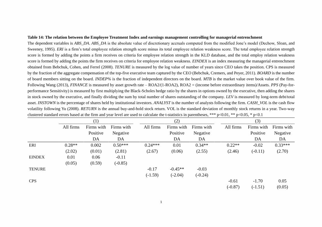
1

Table 14: The relation between the Employee Treatment Index and earnings management controlling for managerial entrenchment

The dependent variables is ABS_DA. ABS_DA is the absolute value of discretionary accruals computed from the modified Jone’s model (Dechow, Sloan, and

Sweeney, 1995). ERI is a firm’s total employee relation strength score minus its total employee relation weakness score. The total employee relation strength

score is formed by adding the points a firm receives on criteria for employee relation strength in the KLD database, and the total employ relation weakness

score is formed by adding the points the firm receives on criteria for employee relation weakness. EINDEX is an index measuring the managerial entrenchment

obtained from Bebchuk, Cohen, and Ferrel (2008). TENURE is measured by the log value of number of years since CEO takes the position. CPS is measured

by the fraction of the aggregate compensation of the top-five executive team captured by the CEO (Bebchuk, Cremers, and Peyer, 2011). BOARD is the number

of board members sitting on the board. INDEP% is the fraction of independent directors on the board. MTB is the market value over book value of the firm.

Following Wang (2013), FINANCE is measured by asset growth rate – ROA2/(1-ROA2), ROA2 = (income before extraordinary items)/Assets. PPS (Pay-for-

performance Sensitivity) is measured by first multiplying the Black-Scholes hedge ratio by the shares in options owned by the executive, then adding the shares

in stock owned by the executive, and finally dividing the sum by total number of shares outstanding of the company. LEV is measured by long-term debt/total

asset. INSTOWN is the percentage of shares held by institutional investors. ANALYST is the number of analysts following the firm. CASH_VOL is the cash flow

volatility following Yu (2008). RETURN is the annual buy-and-hold stock return. VOL is the standard deviation of monthly stock returns in a year. Two-way

clustered standard errors based at the firm and year level are used to calculate the t-statistics in parentheses, *** p<0.01, ** p<0.05, * p<0.1

(1) (2) (3)

All firms Firms with

Positive

DA

Firms with

Negative

DA

All firms Firms with

Positive

DA

Firms with

Negative

DA

All firms Firms with

Positive

DA

Firms with

Negative

DA

ERI 0.28** 0.002 0.50*** 0.24*** 0.01 0.34** 0.22** -0.02 0.33***

(2.02) (0.01) (2.81) (2.67) (0.06) (2.55) (2.46) (-0.11) (2.70)

EINDEX 0.01 0.06 -0.11

(0.05) (0.59) (-0.85)

TENURE -0.17 -0.45** -0.03

(-1.59) (-2.04) (-0.24)

CPS -0.61 -1.70 0.05

(-0.87) (-1.51) (0.05)

1

SIZE 0.02 0.27 -0.18 -0.15* -0.33** -0.18 -0.17* -0.33** -0.20*

(0.27) (1.54) (-1.09) (-1.72) (-2.25) (-1.56) (-1.89) (-2.31) (-1.77)

BOARD -0.10 -0.06 -0.09 -0.09* 0.12 -0.15** -0.08* 0.13* -0.13**

(-0.91) (-0.42) (-1.01) (-1.94) (1.48) (-2.55) (-1.69) (1.72) (-2.32)

INDEP% -1.12 1.15 -1.77** -0.71 0.56 -0.87 -0.78 0.64 -0.92

(-0.99) (0.61) (-2.22) (-1.01) (0.50) (-1.29) (-1.20) (0.59) (-1.49)

MTB 0.14*** -0.02 0.25*** 0.16*** -0.03 0.20*** 0.16*** -0.04 0.20***

(2.62) (-0.43) (2.97) (4.42) (-0.70) (4.99) (4.46) (-0.80) (4.58)

FIN 1.06* 1.32 1.50** 1.36** 3.51*** 1.13** 1.40*** 3.30*** 1.29***

(1.90) (1.24) (2.54) (2.48) (4.36) (2.12) (2.83) (3.91) (2.59)

PPS -0.00 -0.00 -0.00 0.00 0.01 0.00 0.00 0.00 -0.00

(-0.77) (-0.08) (-1.25) (0.59) (1.19) (0.10) (0.02) (0.39) (-0.03)

LEV -1.84 3.58** -2.83** -2.85*** 1.80 -3.27*** -2.91*** 1.76 -3.28***

(-1.28) (2.03) (-1.99) (-3.73) (1.31) (-4.07) (-3.52) (1.27) (-3.70)

ROA -23.30*** 20.43** -33.40*** -25.09*** 18.97*** -30.98*** -24.90*** 19.37*** -30.75***

(-4.03) (2.24) (-7.96) (-5.83) (4.82) (-11.38) (-5.66) (4.84) (-10.54)

INSTOWN 0.03 0.10 0.24 -0.14 0.35 -0.35 -0.04 0.42 -0.24

(0.04) (0.10) (0.21) (-0.26) (0.48) (-0.52) (-0.08) (0.63) (-0.37)

ANALYST 0.03 -0.10** 0.08* 0.04 -0.05 0.07*** 0.04 -0.05 0.07***

(1.01) (-2.43) (1.91) (1.32) (-1.40) (2.67) (1.33) (-1.39) (2.72)

CASH_VOL 5.98*** -1.48 7.79*** 8.67*** 1.53 10.01*** 8.39*** 1.14 9.71***

(4.34) (-0.61) (4.27) (4.08) (0.57) (4.42) (4.10) (0.45) (4.59)

RETURN 0.34 -0.66 1.16 0.54 0.42 0.59* 0.49 0.40 0.50

(0.57) (-0.92) (1.54) (1.59) (0.89) (1.70) (1.54) (0.89) (1.54)

VOL 11.45 24.28*** 6.17 8.25** 15.95*** 3.90 7.83** 15.51*** 3.51

(1.63) (2.85) (0.98) (2.15) (3.21) (0.94) (2.10) (3.33) (0.85)

1

Constant 12.97*** 5.48** 14.95*** 13.38*** 7.84*** 12.73*** 10.66*** 5.09** 12.62***

(8.37) (2.15) (4.36) (7.61) (3.78) (6.53) (6.22) (2.57) (6.21)

Industry fixed

effect

Yes Yes Yes Yes Yes Yes Yes Yes Yes

Year fixed

effect

Yes Yes Yes Yes Yes Yes Yes Yes Yes

Observations 2,910 1,118 1,792 11,627 4,076 7,551 11,970 4,215 7,755

R-squared 0.35 0.39 0.45 0.21 0.21 0.30 0.21 0.21 0.30

1

Table 15: The relation between the Employee Treatment Index and earnings management controlling for labor related factors

The dependent variables is ABS_DA. ABS_DA is the absolute value of discretionary accruals computed from the modified Jone’s model (Dechow, Sloan, and

Sweeney, 1995). ERI is a firm’s total employee relation strength score minus its total employee relation weakness score. The total employee relation strength

score is formed by adding the points a firm receives on criteria for employee relation strength in the KLD database, and the total employ relation weakness

score is formed by adding the points the firm receives on criteria for employee relation weakness. UNION_MEM is the percentage of employees joined in labor

union at the industry level. IND_LABOR is labor expense divided by the number of the employees at the industry level. EMP_OPTION is the value of options

granted to nonexecutive employees per worker estimated by Black-Scholes option pricing model. FIX/AT is the ratio of fixed assets over total assets. SIZE is

the log value of total assets. BOARD is the number of board members sitting on the board. INDEP% is the fraction of independent directors on the board. MTB

is the market value over book value of the firm. Following Wang (2013), FINANCE is measured by asset growth rate – ROA2/(1-ROA2), ROA2 = (income

before extraordinary items)/Assets. PPS (Pay-for-performance Sensitivity) is measured by first multiplying the Black-Scholes hedge ratio by the shares in

options owned by the executive, then adding the shares in stock owned by the executive, and finally dividing the sum by total number of shares outstanding of

the company. LEV is measured by long-term debt/total asset. INSTOWN is the percentage of shares held by institutional investors. ANALYST is the number of

analysts following the firm. CASH_VOL is the cash flow volatility following Yu (2008). RETURN is the annual buy-and-hold stock return. VOL is the standard

deviation of monthly stock returns in a year. Two-way clustered standard errors based at the firm and year level are used to calculate the t-statistics in parentheses,

*** p<0.01, ** p<0.05, * p<0.1

(1) (2) (3)

All firms Firms with

positive DA

Firms with

Negative

DA

All firms Firms with

positive DA

Firms with

Negative

DA

All firms Firms with

positive DA

Firms with

Negative

DA

ERI 0.30*** 0.07 0.36*** 0.23** -0.001 0.34*** 0.39*** 0.30 0.54**

(2.87) (0.45) (2.58) (2.52) (-0.01) (2.74) (2.86) (0.99) (2.22)

UNION_MEM -0.04 -0.08 -0.04

(-0.80) (-0.70) (-0.84)

IND_LABOR 0.002 0.01 0.00

(0.16) (0.52) (0.04)

EMP_OPTION 6.79 -36.92*** 19.63

1

(0.60) (-3.29) (1.40)

SIZE -0.11 -0.31* -0.14 -0.16* -0.33** -0.19* -0.02 -0.01 -0.21

(-1.12) (-1.76) (-1.20) (-1.87) (-2.40) (-1.76) (-0.19) (-0.06) (-1.36)

BOARD -0.07 0.19** -0.13** -0.08* 0.14* -0.13** -0.14* -0.05 -0.13

(-1.29) (2.12) (-2.21) (-1.76) (1.80) (-2.48) (-1.76) (-0.39) (-1.20)

INDEP% -0.88 1.11 -1.38* -0.89 0.41 -0.98 -0.90 1.65 -1.65*

(-1.05) (0.81) (-1.83) (-1.32) (0.38) (-1.52) (-0.97) (1.08) (-1.71)

MTB 0.17*** -0.02 0.21*** 0.16*** -0.04 0.20*** 0.18*** 0.06 0.19***

(4.60) (-0.33) (3.91) (4.55) (-0.77) (4.73) (3.10) (0.97) (3.12)

FIN 1.72*** 3.78*** 1.65*** 1.41*** 3.31*** 1.30*** 2.47*** 4.07*** 2.16***

(2.87) (3.67) (2.96) (2.90) (3.94) (2.67) (3.91) (2.97) (4.34)

PPS 0.00 0.00 0.00 0.00 0.00 -0.00 -0.00 0.00 -0.01

(0.36) (0.46) (0.23) (0.10) (0.66) (-0.04) (-0.79) (0.52) (-1.39)

LEV -3.67*** 0.01 -3.50*** -2.89*** 1.68 -3.20*** -2.92** 2.37 -3.83***

(-4.11) (0.01) (-3.30) (-3.60) (1.22) (-3.73) (-2.10) (1.02) (-4.27)

ROA -26.18*** 20.77*** -31.82*** -24.91*** 19.35*** -30.71*** -23.22*** 19.63** -30.10***

(-6.57) (3.95) (-12.82) (-5.67) (4.82) (-10.47) (-5.90) (2.54) (-11.72)

INSTOWN 0.12 -0.19 0.19 -0.03 0.39 -0.20 -0.03 -0.04 0.28

(0.23) (-0.24) (0.30) (-0.05) (0.57) (-0.31) (-0.06) (-0.04) (0.36)

ANALYST 0.03 -0.09** 0.07*** 0.04 -0.05 0.07*** -0.00 -0.09* 0.05**

(0.89) (-2.08) (2.64) (1.31) (-1.33) (2.65) (-0.16) (-1.89) (1.98)

CASH_VOL 6.76*** -1.66 8.87*** 8.38*** 1.18 9.66*** 5.49*** -1.62 8.11***

(3.62) (-1.52) (4.25) (4.10) (0.47) (4.57) (2.71) (-0.82) (3.33)

RETURN 0.33 -0.19 0.48 0.50 0.37 0.54 0.44 0.14 0.41

(0.86) (-0.42) (1.23) (1.57) (0.83) (1.63) (0.89) (0.23) (0.73)

VOL 7.89* 19.50*** 3.26 8.06** 15.91*** 3.69 11.45*** 23.56*** 6.02

1

(1.84) (3.80) (0.73) (2.18) (3.34) (0.89) (3.35) (3.82) (1.41)

Constant 11.70*** 9.68** 14.66*** 12.74*** 6.82*** 12.57*** 11.80*** 6.08** 13.68***

(5.86) (2.49) (7.02) (7.59) (3.86) (6.54) (6.74) (1.96) (6.00)

Industry fixed

effect

Yes Yes Yes Yes Yes Yes Yes Yes

Year fixed effect Yes Yes Yes Yes Yes Yes Yes Yes

Observations 9,303 3,246 6,057 11,999 4,222 7,777 4,579 1,728 2,851

R-squared 0.22 0.21 0.34 0.21 0.21 0.30 0.23 0.29 0.36

1

Table 16: The relation between the Employee Treatment Index and earnings management controlling for other factors

The dependent variables is ABS_DA. ABS_DA is the absolute value of discretionary accruals computed from the modified Jone’s model (Dechow, Sloan, and

Sweeney, 1995). ERI is a firm’s total employee relation strength score minus its total employee relation weakness score. The total employee relation strength

score is formed by adding the points a firm receives on criteria for employee relation strength in the KLD database, and the total employ relation weakness

score is formed by adding the points the firm receives on criteria for employee relation weakness. RD_INTENSE is the ratio of R&D expense over total assets.

ETHICS is the dummy variable with the value of 1 if the firm is included in Forbes' “The World's Most Ethical Companies" list. KZ_INDEX is the kz index

(Kaplan-Zingales Index) calculated as in Lamont et al. (2001). SIZE is the log value of total assets. BOARD is the number of board members sitting on the

board. INDEP% is the fraction of independent directors on the board. MTB is the market value over book value of the firm. Following Wang (2013), FINANCE

is measured by asset growth rate – ROA2/(1-ROA2), ROA2 = (income before extraordinary items)/Assets. PPS (Pay-for-performance Sensitivity) is measured

by first multiplying the Black-Scholes hedge ratio by the shares in options owned by the executive, then adding the shares in stock owned by the executive, and

finally dividing the sum by total number of shares outstanding of the company. LEV is measured by long-term debt/total asset. INSTOWN is the percentage of

shares held by institutional investors. ANALYST is the number of analysts following the firm. CASH_VOL is the cash flow volatility following Yu (2008).

RETURN is the annual buy-and-hold stock return. VOL is the standard deviation of monthly stock returns in a year. Two-way clustered standard errors based at

the firm and year level are used to calculate the t-statistics in parentheses, *** p<0.01, ** p<0.05, * p<0.1

(1) (2) (3)

All firms Firms with

Positive

DA

Firms with

Negative DA

All firms Firms with

Positive

DA

Firms with

Negative DA

All firms Firms with

Positive

DA

Firms with

Negative DA

ERI 0.27** -0.13 0.41*** 0.04 -0.17 0.18** 0.24** -0.04 0.37**

(2.12) (-0.67) (2.83) (0.46) (-0.89) (1.98) (2.23) (-0.24) (2.53)

RD_INTENSE -1.16*** -0.66 -1.46***

(-2.84) (-0.27) (-3.74)

ETHICS -0.10 -0.77 -0.10

(-0.17) (-0.80) (-0.18)

KZ_INDEX 0.001** 0.00 0.00

(1.98) (1.39) (1.61)

1

SIZE 0.04 -0.39* 0.09 -0.20* -0.48*** -0.24 -0.10 -0.26** -0.15

(0.32) (-1.65) (0.74) (-1.84) (-3.63) (-1.34) (-1.20) (-2.01) (-1.22)

BOARD -0.11 0.23** -0.22*** -0.09* 0.14 -0.12** -0.08 0.14* -0.14**

(-1.56) (1.98) (-2.76) (-1.77) (1.62) (-2.06) (-1.40) (1.76) (-2.30)

INDEP% -0.16 0.97 -0.52 0.04 1.78 -0.17 -0.70 0.73 -0.93

(-0.19) (0.70) (-0.57) (0.03) (1.00) (-0.14) (-0.95) (0.63) (-1.29)

MTB 0.14*** -0.05 0.18*** 0.15*** -0.10* 0.18*** 0.16*** -0.04 0.20***

(3.17) (-0.87) (3.27) (3.56) (-1.92) (4.21) (4.48) (-0.69) (4.19)

FIN 2.04*** 3.68*** 2.36*** 0.43 3.33*** -0.03 1.44*** 3.28*** 1.38**

(3.15) (3.23) (2.90) (0.74) (3.34) (-0.04) (2.95) (3.62) (2.48)

PPS 0.00 0.01 0.00 0.00 0.00 0.01 0.00 0.00 0.00

(1.13) (0.93) (0.31) (1.32) (0.28) (1.55) (0.31) (0.63) (0.45)

LEV -3.82*** 1.93 -4.16*** -2.08* 2.19 -2.37* -3.02*** 1.44 -3.41***

(-3.10) (0.93) (-3.44) (-1.91) (1.12) (-1.70) (-3.76) (0.96) (-3.76)

ROA -27.29*** 23.08*** -33.45*** -26.16*** 23.46*** -31.38*** -24.69*** 19.46*** -30.54***

(-6.70) (4.36) (-13.10) (-4.25) (4.75) (-7.77) (-5.20) (4.35) (-9.50)

INSTOWN -0.76 -1.12 -0.56 -0.10 0.06 -0.34 0.27 0.62 0.08

(-1.21) (-1.16) (-0.70) (-0.16) (0.06) (-0.52) (0.55) (0.85) (0.11)

ANALYST 0.04 -0.07 0.08*** 0.06 -0.05 0.10** 0.02 -0.07* 0.06**

(1.37) (-1.31) (2.81) (1.45) (-0.88) (2.48) (0.79) (-1.88) (2.46)

CASH_VOL 6.03*** -0.28 6.77*** 11.73*** 7.93 7.78** 8.12*** 1.48 9.03***

(2.97) (-0.12) (2.90) (3.00) (1.45) (2.25) (3.64) (0.49) (4.01)

RETURN 0.77* 0.33 0.95* 0.65** 0.70 0.76*** 0.45 0.24 0.49

(1.66) (0.47) (1.86) (2.21) (0.84) (3.28) (1.27) (0.51) (1.43)

VOL 9.92*** 19.62*** 5.37 7.59 15.80** 3.19 7.86* 16.22*** 3.22

(2.87) (3.80) (1.46) (1.55) (2.42) (0.52) (1.90) (2.86) (0.77)

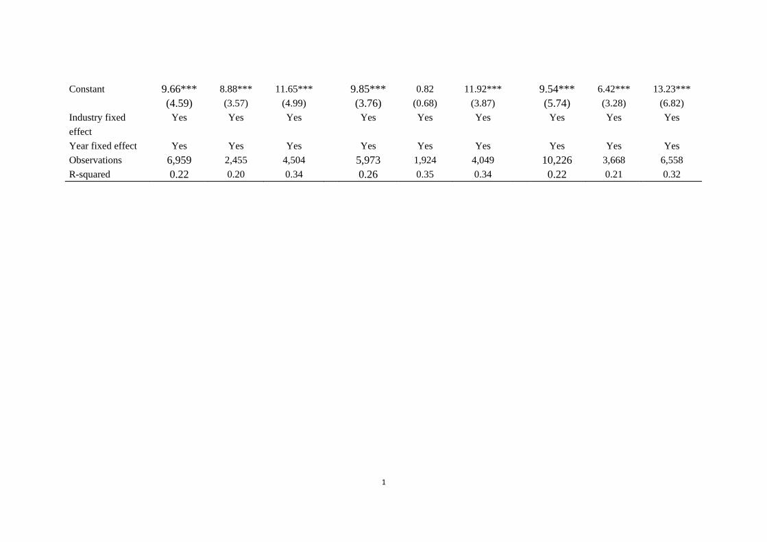
1

Constant 9.66*** 8.88*** 11.65*** 9.85*** 0.82 11.92*** 9.54*** 6.42*** 13.23***

(4.59) (3.57) (4.99) (3.76) (0.68) (3.87) (5.74) (3.28) (6.82)

Industry fixed

effect

Yes Yes Yes Yes Yes Yes Yes Yes Yes

Year fixed effect Yes Yes Yes Yes Yes Yes Yes Yes Yes

Observations 6,959 2,455 4,504 5,973 1,924 4,049 10,226 3,668 6,558

R-squared 0.22 0.20 0.34 0.26 0.35 0.34 0.22 0.21 0.32