Elementary Number Theory - Department of Mathematicskab/509/bigbook.pdf · D.IV Gauß’ Lemma . ....
415
Elementary Number Theory Peter Hackman HHH Productions November 1, 2009
Transcript of Elementary Number Theory - Department of Mathematicskab/509/bigbook.pdf · D.IV Gauß’ Lemma . ....

Elementary Number Theory
Peter HackmanHHH Productions
November 1, 2009

ii
c© P Hackman, 2009.

Contents
Preface ix
A Divisibility, Unique Factorization 1
A.I The gcd and Bezout . . . . . . . . . . . . . . . . . . . . . . 1
A.II Two Divisibility Theorems . . . . . . . . . . . . . . . . . . 7
A.III Unique Factorization . . . . . . . . . . . . . . . . . . . . . 9
A.IV Residue Classes, Congruences . . . . . . . . . . . . . . . . . 12
A.V Order, Little Fermat, Euler . . . . . . . . . . . . . . . . . . 21
A.VI A Brief Account of RSA . . . . . . . . . . . . . . . . . . . . 33
B Congruences. The CRT. 37
B.I The Chinese Remainder Theorem . . . . . . . . . . . . . . 37
B.II Euler’s Phi Function Revisited . . . . . . . . . . . . . . . . 44
* B.III General CRT . . . . . . . . . . . . . . . . . . . . . . . . . . 48
B.IV Application to Algebraic Congruences . . . . . . . . . . . . 53
B.V Linear Congruences . . . . . . . . . . . . . . . . . . . . . . 54
B.VI Congruences Modulo a Prime . . . . . . . . . . . . . . . . . 56
B.VII Modulo a Prime Power . . . . . . . . . . . . . . . . . . . . 60
C Primitive Roots 69
iii

iv CONTENTS
C.I False Cases Excluded . . . . . . . . . . . . . . . . . . . . . 69
C.II Primitive Roots Modulo a Prime . . . . . . . . . . . . . . . 72
C.III Binomial Congruences . . . . . . . . . . . . . . . . . . . . . 76
C.IV Prime Powers . . . . . . . . . . . . . . . . . . . . . . . . . . 81
C.V The Carmichael Exponent . . . . . . . . . . . . . . . . . . . 88
* C.VI Pseudorandom Sequences . . . . . . . . . . . . . . . . . . . 92
C.VII Discrete Logarithms . . . . . . . . . . . . . . . . . . . . . . 94
* C.VIII Computing Discrete Logarithms . . . . . . . . . . . . . . . 95
D Quadratic Reciprocity 107
D.I The Legendre Symbol . . . . . . . . . . . . . . . . . . . . . 107
D.II The Jacobi Symbol . . . . . . . . . . . . . . . . . . . . . . 118
D.III A Cryptographic Application . . . . . . . . . . . . . . . . . 123
D.IV Gauß’ Lemma . . . . . . . . . . . . . . . . . . . . . . . . . 123
D.V The “Rectangle Proof” . . . . . . . . . . . . . . . . . . . . 127
D.VI Gerstenhaber’s Proof . . . . . . . . . . . . . . . . . . . . . 129
* D.VII Zolotareff’s Proof . . . . . . . . . . . . . . . . . . . . . . . 131
E Some Diophantine Problems 143
E.I Primes as Sums of Squares . . . . . . . . . . . . . . . . . . 143
E.II Composite Numbers . . . . . . . . . . . . . . . . . . . . . . 150
E.III Another Diophantine Problem . . . . . . . . . . . . . . . . 156
E.IV Modular Square Roots . . . . . . . . . . . . . . . . . . . . . 160
E.V Applications . . . . . . . . . . . . . . . . . . . . . . . . . . 165
F Multiplicative Functions 167
F.I Definitions and Examples . . . . . . . . . . . . . . . . . . . 167

CONTENTS v
F.II The Dirichlet Product . . . . . . . . . . . . . . . . . . . . . 169
F.III Mobius Inversion . . . . . . . . . . . . . . . . . . . . . . . . 172
* F.IV Two More Results . . . . . . . . . . . . . . . . . . . . . . . 175
F.V Primitive Roots, Again . . . . . . . . . . . . . . . . . . . . 179
F.VI A Combinatorial Application . . . . . . . . . . . . . . . . . 181
F.VII The Sum of Divisors . . . . . . . . . . . . . . . . . . . . . . 184
F.VIII Cyclotomic Polynomials . . . . . . . . . . . . . . . . . . . . 187
G Continued Fractions 195
G.I Motive, Definitions . . . . . . . . . . . . . . . . . . . . . . . 195
G.II Basic Theorems . . . . . . . . . . . . . . . . . . . . . . . . 199
* G.III Negative Irrationalities . . . . . . . . . . . . . . . . . . . . 205
G.IV Best Rational Approximation . . . . . . . . . . . . . . . . . 206
G.V Where Are the “Continued Fractions”? . . . . . . . . . . . 210
G.VI Finite Continued Fractions . . . . . . . . . . . . . . . . . . 213
G.VII Cornacchia’s Algorithm . . . . . . . . . . . . . . . . . . . . 216
H “QCF” and Pell’s Equation 223
H.I An Algorithm for Quadratic Irrationalities . . . . . . . . . . 223
H.II Conjugates . . . . . . . . . . . . . . . . . . . . . . . . . . . 227
H.III x2 −Dy2 = ±1 . . . . . . . . . . . . . . . . . . . . . . . . . 228
H.IV x2 −Dy2 = N . . . . . . . . . . . . . . . . . . . . . . . . . 240
H.V Inequalities . . . . . . . . . . . . . . . . . . . . . . . . . . . 244
H.VI Periodicity . . . . . . . . . . . . . . . . . . . . . . . . . . . 245
* H.VII Periodicity, Continued . . . . . . . . . . . . . . . . . . . . . 247
J Special Topics on Continued Fractions 255

vi CONTENTS
J.I Matrix Notation . . . . . . . . . . . . . . . . . . . . . . . . 255
J.II Equivalent Quadratic Irrationalities . . . . . . . . . . . . . 257
J.III Equivalence and Continued Fractions . . . . . . . . . . . . 258
* J.IV An Alternative Approach . . . . . . . . . . . . . . . . . . . 263
J.V Reciprocal Expansions . . . . . . . . . . . . . . . . . . . . . 266
J.VI Selfreciprocity, Partial Quotients . . . . . . . . . . . . . . . 268
J.VII Symmetry of the Pk, Qk . . . . . . . . . . . . . . . . . . . . 271
* J.VIII Moving Forward One Period . . . . . . . . . . . . . . . . . 271
* J.IX Running a Period Backwards . . . . . . . . . . . . . . . . . 275
* J.X More on Pell-Like Equations . . . . . . . . . . . . . . . . . 277
J.XI More on x2 −Dy2 = N . . . . . . . . . . . . . . . . . . . . 283
K Z[i], Other Number Rings 291
K.I Preparations . . . . . . . . . . . . . . . . . . . . . . . . . . 291
K.II Unique Factorization in Z[i] . . . . . . . . . . . . . . . . . . 296
K.III The Number of Representations . . . . . . . . . . . . . . . 306
K.IV Z[−12
+ i√
32
] . . . . . . . . . . . . . . . . . . . . . . . . . . 308
L Primality and Factorization 313
L.I Introduction . . . . . . . . . . . . . . . . . . . . . . . . . . 313
L.II Special Numbers, Special Factors . . . . . . . . . . . . . . . 314
L.III Trial Division . . . . . . . . . . . . . . . . . . . . . . . . . . 317
L.IV Lists of Primes . . . . . . . . . . . . . . . . . . . . . . . . . 317
L.V Fast Exponentiation . . . . . . . . . . . . . . . . . . . . . . 320
L.VI Primality: Fermat and Miller-Rabin . . . . . . . . . . . . . 321
L.VII Lehmer, Lucas, Pocklington . . . . . . . . . . . . . . . . . . 327
L.VIII Factoring: Pollard p− 1 . . . . . . . . . . . . . . . . . . . . 335
CONTENTS vii
L.IX Factoring, Pollard rho . . . . . . . . . . . . . . . . . . . . . 336
L.X “Waiting For a Square” . . . . . . . . . . . . . . . . . . . . 344
L.XI CFRAC . . . . . . . . . . . . . . . . . . . . . . . . . . . . . 347
L.XII Elimination Modulo 2 . . . . . . . . . . . . . . . . . . . . . 354
L.XIII Quadratic Sieve . . . . . . . . . . . . . . . . . . . . . . . . 358
L.XIV Lucas Sequences and Primality . . . . . . . . . . . . . . . . 362
L.XV Mersenne Numbers . . . . . . . . . . . . . . . . . . . . . . 371
L.XVI Lucas and Modular Square Roots . . . . . . . . . . . . . . 374
L.XVII Scalar Formulas . . . . . . . . . . . . . . . . . . . . . . . . 377
Bibliography 381
Tables 389

viii CONTENTS

Preface
My last new assignment at Linkoping University was to a course in Elemen-tary Number Theory. While somewhat removed from my algebraic interestsand competence, that course (which I conducted for five years) turned outto be an extremely rewarding and challenging experience, largely due to theenthusiasm of the students.
Never content to just copy text books, I put a lot of energy into findingnew proofs, new ways of organizing the material, and some at least unusualtopics. This quest for inspiration produced a lot of notes that I decided tocompile into a short text on retiring from the University. As you might haveguessed, the project grew into a full-size book.
What I hoped to contribute to the existing literature is a perhaps slimmerand more affordable volume. At the same time I wished to include someexciting and challenging, yet completely elementary, material not found incurrent texts.
“Elementary” means that almost no Analysis is used, and almost no “Ab-stract” Algebra. Algebra really becomes abstract only with the introductionof techniques like homomorphisms, direct sums and quotient constructions.We do, however, speak of (number) rings, fields, and residue classes of inte-gers, and their arithemetic.
Among the more unusual material is a reasonably complete account of Cor-nacchia’s algorithm for solving x2 +Dy2 = p, using Euclid’s Algorithm, andthat of Lagrange (revived by Matthews and Mollin) for x2 −Dy2 = N , us-ing infinite continued fractions. There are strong analogies between the twotheories, which I emphasize by using exactly the same wording in severalparallel passages. Modular square roots is another of my favorite topics,and I present two algorithms for them, that of Berlekamp and the one usingLucas sequences (or, equivalently, Cipolla’s algorithm) each exploiting someinteresting theoretical item.
ix

x PREFACE
To keep the material within bounds I had to make some clear decisions whatnot to include. One main decision was to not give proofs of the statistics andcomplexity of algorithms. There are comprehensive accounts in the books byRiesel, Bach-Shallit, and Crandall-Pomerance cited in the Bibliography.
Another decision was to give fewer applications. The motivational valueof applications does not depend on their quantity; besides, who wants tocompete with such excellent texts (in Cryptography) as Trappe-Washington,or Buchmann? To be sure, almost all of the math relevant to these accounts,is included here. Whenever I found an application worthy of inclusion it wasusually because it strengthened some of the main theoretical ideas of thetext.
A few words about style. For the most part I stick to the strict Definition-Example-Theorem-Proof-Example format simply because I want to make itclear where things begin and end. Also, many readers (like me) will want toskip longer proofs on a first reading.
Having dabbled in journalism I try to paragraph and display often. I havealso tried to minimize the number of cross-references. Further , by numberingeverything in one sequence, and boxing theorems and definitions I hope tomake it easier on the reader. As I never refer back to a subsection, these areun-numbered.
Finally, there is no numbering of equations, as reference to them is strictlylocal. They are labeled by one to three stars. I simply hate references like“we now return to the study of the differential operator (17) in Section XVIIof Chapter Q” (that operator of course being the Laplacian).
Books are referred to by author name. Very few articles are cited; in thesecases I give full reference in the text, but I have also collected them at theend of the text.
I strongly advocate the use of computers as a means of generating and inves-tigating examples. To really understand an algorithm, or a result, it helpsto program it. There are suggestions for computer projects, ranging in com-plexity from a few lines to maybe one or two pages.
Hopefully the suggested projects still allow the math to dominate over moredelicate programming issues. Ideally much more work should be spent onchecking and tracing, and varying the input and the parameters, than on de-vising the program. This text is not conceived as a book on “computational”number theory.

xi
There are “suggestions for computing” sprinkled throughout the exercises,and the reader will often have the option to use programs of his own designor rely on existing packages, such as Maple, Mathematica, and PARI. Toascertain the feasibility of the algorithms to anyone with moderate program-ming experience I have written and run simple programs on just about anyalgorithm persented here,
In my courses students could choose their programming language freely (butmulti-precision arithmetic is imperative). A very popular language is Python,which is the language I used in constructing and checking all my examples,and the tables at the end of the book.
You are never alone. Students, friends, and former colleagues helped andinspired me in several ways. Mikael Langer and Jan-Ake Larsson graciouslyaided the traumatic transition from Plain TEX to LATEX. Hans Lundmark andNiels Moller read large chunks of the text and offered suggestions and cor-rections, immensely enhancing the readability of the text. Hans also helpedme with a number of programming issues.
Par Kurlberg (Erdos number two) read an early version of Chapter L, andoffered valuable insights and comments. I am also grateful to him for intro-ducing me to the Python programming language several years ago. I havealso received valuable input and support from an email correspondence withKeith Matthews of Brisbane, Australia.
Finally, I wish to acknowledge the generous help from Thomas Bellman inexplaining some of the mysteries of Python.
It is my hope that this text will give something back to the subject thatbrightened the last five years of my career.
Linkoping, Sweden, October 2007,
Peter Hackman

xii PREFACE

Chapter A
Divisibility, UniqueFactorization
A.I The gcd and Bezout
We assume you are familiar with the integers, their addition, subtraction, andmultiplication. We will later introduce algebraic integers, especially complexintegers. When we want to distinguish ordinary integers from more generalones we use the expression “rational integer”.
We will make repeated use of division with remainder: Given integers n > 0,and m, there are (unique) integers q and r, 0 ≤ r < n, such that m = qn+ r.
The existence of q, r is easily proved. The set of numbers m − qn, q ∈ Zcontains non-negative numbers. If m ≥ 0, m itself is one such number. Ifm < 0, pick m−mn. r is then chosen as the smallest non-negative number ofthe form m−qn. If r ≥ n, then m−(q+1)n is smaller and still non-negative,contradiction.
We have invoked the Well-ordering Principle:
“Every non-empty set of non-negative integers contains a smallest element.”
On a few occasions we use the absolutely least remainder, satisfying |r| ≤n/2, or more precisely, −n/2 < r ≤ n/2. If m = qn + r, n/2 < r < n, thenalso m = (q + 1)n+ (r − n), with −n/2 < r − n < 0.
We start with a very simple definition:
1

2 CHAPTER A. DIVISIBILITY, UNIQUE FACTORIZATION
A.I.1 Definition. The integer m is a factor of the integer n, or mdivides n, or n is divisible by m, if there is an integer q, satisfyingn = mq.
Notation: m|n. The notation for “m does not divide n” is m - n.
The number 0 is obviously divisible by any integer. If a divides m and n,then a also divides all rm, sn, rm+ sn, for integers r, s.
A.I.2 Definition. The greatest common divisor of the two integersm,n (not both =0) is the greatest integer d which divides both. Notation:d = (m,n) or d = gcd(m,n).
A.I.3 Example. (8,−4) = 4, (7, 11) = (4, 9) = 1. �
By convention (0, 0) = 0. In all other cases (m,n) is positive (“positive” inthis text means “> 0”).
For m 6= 0 obviously (m, 0) = |m|, the absolute value of m.
We have defined the greatest common divisor with reference to the usualtotal ordering of the integers.
More significantly, it is also the greatest common divisor according to thepartial ordering of divisibility. That is, every other common divisor of m andn is not only smaller than d = (m,n), but also divides it.
That is part c) of the following Theorem:
A.I.4 Theorem.
a) Let d = (m,n). There are integers r, s such that d = rm+ sn.
b) The linear Diophantine equation e = xm + yn is solvable in integersx, y if and only if (m,n)|e.

A.I. THE GCD AND BEZOUT 3
c) Every common divisor of m,n divides their greatest common divisor.
Proof. We first show how b) follows from a). If d = (m,n), d = rm + sn,and e = qd, then e = qrm+ qsn, proving one direction of the equivalence.
Conversely, assume e = xm+ yn. Since d = (m,n) divides xm, yn, xm+ ynit follows immediately that d|e. This was the easier direction, as we neverused a).
For the proof of a) we can assume that m,n 6= 0. Let d = rm + sn bethe least positive number of that form. Such integers do indeed exist, e.g.,|m|, |n|, and every non-empty set of positive integers has a smallest element.
We first show that d divides both m and n. Perform the division:
m = qd+ t = q(rm+ sn) + t; 0 ≤ t < d.
The remainder t = (1− qr)m− qsn is of the same form as d but smaller, andt ≥ 0. The minimality of d thus forces t = 0, i.e., d|m.
In the same manner we show d|n. But every common factor of m,n obviouslydivides d = rm + sn. Therefore, d must be divisible by all common factorsin m,n, hence d is the greatest among them. This finishes the proof of bothparts a) and c) of the Theorem. �
Remark: The word Diophantine always refers to solvability in integers.
A.I.5 Definition. The integers m,n 6= 0 are relatively prime if(m,n) = 1, i.e., if their only common factors are ±1.
For relatively prime m,n, by the Theorem above, the equation xm+ yn = 1,Bezout’s Identity, is solvable in integers. Trivially, xm+ ny = 1, for integersx, y, implies (m,n) = 1.
The Euclidean Algorithm is a very old and fast method for determining(m,n). If m ≥ n, the number of bit operations required is quadratic inthe number of bits in the binary representation of m. For detailed discus-sions of complexity questions of this kind I refer to more comprehensive textsin Number Theory.

4 CHAPTER A. DIVISIBILITY, UNIQUE FACTORIZATION
We explain by example why Euclid gives the greatest common divisor. Thenwe redo our solution in a way that simultaneously, in the case (m,n) = 1,solves Bezout’s identity.
A closer analysis of our Examples could be formalized into a computationalproof of our previous Theorem.
A.I.6 Example (Euclidean Algorithm). Let us compute (37, 11) = 1.We start by dividing one number by the other:
37 = 3 · 11 + 4.
By the principles we have used repeatedly above, each common factor of 37and 11 is also one of 11 and 4 = 1 · 37− 3 · 11.
On the other hand, each common factor of 11 and 4 is one of 37 = 3 ·11+1 ·4and 4 as well. Hence, the two pairs 37, 11, and 11, 4, have the same commonfactors. In particular their greatest common divisors are the same.
The pattern continues:
37 = 3 · 11 + 4
11 = 2 · 4 + 3
4 = 1 · 3 + 1
whence
(37, 11) = (11, 4) = (4, 3) = (3, 1) = 1.
The following is a simple example with (m,n) > 1:
77 = 3 · 21 + 14
21 = 1 · 14 + 7
14 = 2 · 7 + 0
whence
(77, 21) = (21, 14) = (14, 7) = (7, 0) = 7.
�
Clearly, the gcd is the last non-zero remainder in this division scheme.

A.I. THE GCD AND BEZOUT 5
A.I.7 Example (Extended Euclid). We now show how to modify the al-gorithm so as to simultaneously solve Bezout (“Extended Euclidean Algo-rithm”). We start with two relations no one could possibly challenge:
1 · 37 + 0 · 11 = 37
0 · 37 + 1 · 11 = 11.
We then divide the first right member by the second: 37−3 ·11 = 4 and per-form the corresponding row operation: “equation 1 minus 3 times equation2”.
We arrive at 1 · 37− 3 · 11 = 4.
We now drop the first equation above and add the one just derived:
0 · 37 + 1 · 11 = 11
1 · 37− 3 · 11 = 4
These we combine in the same way as above. Divide: 11 − 2 · 4 = 3. Form“(new) equation 1 minus 2 times (new) equation 2”, yielding−2·37+7·11 = 3.After one more step we arrive at:
1 · 37 + 0 · 11 = 37
0 · 37 + 1 · 11 = 11 37− 3 · 11 = 4
1 · 37− 3 · 11 = 4 11− 2 · 4 = 3
−2 · 37 + 7 · 11 = 3 4− 3 = 1
3 · 37− 10 · 11 = 1
and we have solved Bezout! �
Note that each step only requires that the coefficients of two equations bestored. After division, the first equation is dropped, the second equationmoves to the top, and a new equation takes its place. The algorithm iseminently programmable.
A.I: Exercises
1. Solve Bezout for each of the following pairs: (17,29), (33,81), (48,81).

6 CHAPTER A. DIVISIBILITY, UNIQUE FACTORIZATION
2. Using the identity Xnd−1 = (Xd−1)(X(n−1)d+X(n−2)d+· · ·+1), determinethe gcd’s (215−1, 23−1), (210−1, 215−1), (215−1, 29−1), or, quite generally,(2m − 1, 2n − 1). If you represent these numbers in binary, what will Euclidlook like?
3. Let m,n be integers. Show that
(m,n) =(
m− n
2, n
)if both are odd.
What can be said about (2m, 2n), and (2m,n), assuming n odd in the secondcase?
From these observations, devise an alternative Euclidean algorithm usingno divisions (division by 2 is a right shift in binary representation, checkingparity is a bitwise “and” with 1).

A.II. TWO DIVISIBILITY THEOREMS 7
A.II Two Divisibility Theorems
We will make repeated use of the following two Divisibility Theorems. Notethe decisive role played by Bezout.
A.II.1 Theorem (First Divisibility Theorem). If m|ab, and(m, a) = 1, then m|b.
Proof. Bezout gives us x, y with xm + ya = 1. Multiplication by b yieldsb = bxm + yab. The terms of the right member are divisible by m, the firstone trivially, the second one by asssumption. Hence m divides their sum,i.e., m|b. �
A.II.2 Theorem (Second Divisibility Theorem). If both m,n di-vide a, and (m,n) = 1, then their product mn divides a.
Proof. The divisibility assumptions may be written n|a = qm. We arealso assuming (m,n) = 1. The previous Theorem immediately gives n|q,hence mn|mq = a. �
A.II: Exercises
1. If x divides my, ny, and (m,n) = 1, then x divides y.
2. Let a, b be relatively prime integers. Suppose x0a+y0b = 1. Find the generalsolution to the linear Diophantine equation xa + yb = 1. Then generalize tothe situation (a, b) = d > 1.
3. Suppose the positive integers m,n satisfy n3 + n = m4. Show that m,n areeven; hence or otherwise, 16|n.
4. The polynomial f(X) = a0Xd + a1X
d−1 + · · · + ad has integer coefficients.Let X = p/q, (p, q) = 1, be a rational root. Show that p|ad, and q|a0. Hint:rewrite the relation f(p/q) = 0 as a relation between integers.

8 CHAPTER A. DIVISIBILITY, UNIQUE FACTORIZATION
5. A common way of factoring a number is to write it as a difference of twosquares: a2 − b2 = (a + b)(a− b).
(a) Let h be an odd positive integer. Show that
24k+2 + 15
, k > 1, and 32h+2 + 3h+1 + 1
are composite. Hint: a2 + b2 = (a + b)2 − 2ab.
(b) In the case of the first number of the previous item, you will be ableto decompose 24k+2 + 1 into two factors one of which is divisible by5. Which of them? The answer will depend on the remainder of k ondivision by some small positive integer. Determine the cases.
(c) Show that a2 + 4a is composite, if a is an odd positive integer > 1(trivial for even a).

A.III. UNIQUE FACTORIZATION 9
A.III Unique Factorization
We recall a familiar concept.
A.III.1 Definition. A prime number is an integer p > 1 divisible onlyby the trivial factors ±1 and ±p.
The set of prime numbers is infinite. If p1 < p2 < · · · < pd are prime numbers,then the smallest divisor p > 1 of 1 + p1p2 · · · pd is a prime number differentfrom all of these.
Lest you jump to conclusions, note that 1+2 ·3 ·5 ·7 ·11 ·13 = 30031 = 59 ·509is composite.
You will be familiar with the following results, but maybe not with theirproofs.
A.III.2 Theorem (Prime Factorization, Existence). Every inte-ger n > 1 is a product of prime numbers.
Proof. Induction on n. Let p be the smallest divisor > 1 of n. It is aprime number. If p = n we are through. Otherwise we apply induction tothe quotient 1 < n/p < n. �
The uniqueness part is preceded by a little Lemma, a special case of our FirstDivisibility Theorem (A.II.1).
A.III.3 Lemma. Let q be a prime number, a, b integers. Assume thatq divides their product ab. Then q divides either a or b.
Proof. If q does not divide a, then (q, a) = 1 is the only possibility. TheFirst Divisibility Theorem then immediately gives q|b. �

10 CHAPTER A. DIVISIBILITY, UNIQUE FACTORIZATION
A.III.4 Corollary. If n = p1 · p2 · p3 · · · pk is a prime factorization of n,and the prime number q divides n, then q equals one of the pj’s.
Proof. If k = 1, then obviously q = p1. If k > 1, and q 6= p1, then qdivides p2 · · · pk and we can proceed by induction on k. �
A.III.5 Theorem (Unique Factorization). The prime factorizationof n > 1 is unique, up to the order of the factors.
Proof. Suppose n = p1 · · · pk = q1 · · · ql, k ≤ l, are two prime factorizationsof n. If k = 1, then n is a prime number, and obviously l = 1, q1 = p1.
If k > 1, then q1 equals one of the pj’s, say q1 = pj, by the Corollary. Dividingboth members by this common factor we are reduced to studying the shorterfactorizations of n/pj, and the result now follows by induction on k. �
A.III: Exercises
1. If u, v, x > 0 are integers, (u, v) = 1, and uv = x2, then u, v, too, are perfectsquares. Can you prove this without using unique factorization in primefactors? Generalize to arbitrary powers.
2. Let a, b be positive integers satisfying aj = bk for positive and relativelyprime integers j, k. Show that a = rk, b = rj for some positive integer r.
3. Let p be a prime number, n a positive integer. Let vp(n) denote the largestinteger k ≥ 0 such that pk|n. Further, let the floor bac denote the largestinteger m ≤ a.
(a) Express the number of integers m, 1 ≤ m ≤ n, divisible by p, as afloor.
(b) Express vp(n!) as a sum of floors.
(c) Find the number of final zeros, v5(n!), for n = 2006.

A.III. UNIQUE FACTORIZATION 11
4. Pythagorean triples. Suppose x, y, z are positive integers satisfying x2+y2 =z2. Suppose also that they are without common factors > 1, forcing themto be pairwise relatively prime. We say that x, y, z is a proper, or primitive,Pythagorean triple.
Suppose further, as we may, that x is odd, and y is even. From the rela-tion (z − x)(z + x) = y2 deduce a parametric representation of all properPythagorean triples x, y, z. Start by determining (x + z, z − x).
(You may wish to connect this with the rational representation of the pointson the circle x2 + y2 = R2 obtained by intersecting the circle with a linethrough the point (−R, 0) of given rational slope – your parameters will havea familiar trigonometric interpretation.)
5. Let a0, a1, . . . , an−1 be given (positive) distinct integers. Show that thereare (positive) integers D,E such that the numbers Daj + E are pairwiserelatively prime.
Hint: If p is a prime dividing two of the numbers Daj+E, then it also dividestheir difference. Construct D as the product of certain prime numbers, andlet E be some other prime.

12 CHAPTER A. DIVISIBILITY, UNIQUE FACTORIZATION
A.IV Residue Classes, Congruences
A.IV.1 Definition. We fix an integer n > 0. The (residue) class ofm, modulo n, denoted [m], or m + (n), is the set of all numbers of theform m+ rn, r ∈ Z.
Note that the class symbol [m] contains no reference to the given integer,the modulus n. Some writers affix a subscript n to the class symbol in caseof ambiguity. In that case I prefer the notation m+ (n). For one thing, it iseasier to type.
The class of zero, modulo 3, is [0] = {. . . ,−12,−9,−6,−3, 0, 3, 6, . . . } con-sisting of all multiples of 3. You can think of them as equidistant points onthe line, 3 units apart. Each of the numbers is said to represent the class.
The class of 1,
[1] = {. . . ,−11,−8,−5,−2, 1, 4, 7, . . . },
is obtained by shifting the zero class one step to the right along the line. Itconsists of the numbers that yield the remainder 1, on division by 3.
Another shift to the right gives us the class
[2] = {. . . ,−10,−7,−4,−1, 2, 5, . . . }.
These are the numbers yielding the remainder 2 on division by 3.
A third shift gives us back the class [3] = [0].
For general n > 0 we obtain n different, and pairwise disjoint, classes
[0], [1], [2], . . . , [n− 1].
Shifting one class n unit steps in either direction gives us back the same class.
Each integer belongs to exactly one class modulo n. We say that the n classesconstitute a partition of the set Z.
Those who have taken a course in Discrete Math will ask, what is the equiv-alence relation belonging to this partition. More concretely, the question is:when (for given n > 0) is a+ (n) = b+ (n)?
A.IV. RESIDUE CLASSES, CONGRUENCES 13
Equality clearly holds if and only if either of a and b belongs to the class ofthe other, i.e., if a and b differ by a multiple of n.
Another way of expressing this condition is that n divide the difference:n|(a− b).
A third way of phrasing the condition is that a and b leave the same remainderon division by n.
We introduce a name and notation for this condition.
A.IV.2 Definition. The integers a and b are congruent modulo n ifn|(a− b). Notation: a ≡ b (mod n).
Anyone familiar with the concept (from Discrete Math) verifies easily thatthis is indeed an equivalence relation (symmetric, transitive, reflexive). Oth-ers can safely ignore the issue.
More important is the fact that we can do arithmetic on classes.
A.IV.3 Lemma. Fix n > 0. Assume a1 ≡ b1 (mod n), a2 ≡ b2(mod n). Then a1 ± a2 ≡ b1 ± b2 (mod n) and a1 · a2 ≡ b1 · b2 (mod n).
Proof. We content ourselves with proving the second property – the firstone is even easier.
We are assuming that n|(a1 − b1) and n|(a2 − b2). Then n also dividesa1a2 − b1b2 = a2(a1 − b1) + b1(a2 − b2). �
In words, the Lemma just proved states that the class of a sum, difference,or product of two numbers depends only on the class of the terms or factors.
Therefore the following definition is meaningful:
A.IV.4 Definition.
[a]± [b] = [a± b]; [a] · [b] = [a · b].

14 CHAPTER A. DIVISIBILITY, UNIQUE FACTORIZATION
As the arithmetic operations are derived from operations on integers one eas-ily proves that the usual laws hold. Addition and multiplication are commu-tative (independent of the order of the terms or factors). They are associative(no need for parentheses). And we have a distributive law :
[a]([b] + [c]) = [a][b] + [a][c].
A.IV.5 Example. Most of the time we want to represent our classes bythe numbers 0, 1, . . . n− 1. Adding, subtracting or multiplying two represen-tatives usually leads outside this set; we remedy this by dividing by n andkeeping the remainder.
For our first set of examples we fix n = 8. Then
[4] + [6] = [10] = [2]; [4] · [6] = [24] = [0]; [5] · [9] = [45] = [5],
as 45 = 5 · 8 + 5. Finally, [5] · [5] = [25] = [1].
In the second example the multiplication of two non-zero classes yields thezero class. We say that the non-zero classes [4] and [6] are zero-divisors.If the product of two classes equals [1] they are said to be inverses of oneanother; the two classes are then invertible. For n = 8 the classes of 1,3,5,7are their own inverses.
For n = 7 all non-zero classes are invertible:
[1] · [1] = [1]; [2] · [4] = [1]; [3] · [5] = [1]; [6] · [6] = [1].
Notation (n = 7): [3]−1 = [5]; [5]−1 = [3]. We sometimes use the notationa−1 for a representative of the class [a]−1.
�
Let us record the formal definitions:
A.IV.6 Definition.
a) The class [a] modulo n > 0 is invertible if there exists a class [b]satisfying [a][b] = [1].
b) The class [a] 6= [0] is a zero-divisor if there exists a class [b] 6= [0]satisfying [a][b] = [0].

A.IV. RESIDUE CLASSES, CONGRUENCES 15
How do we recognize invertible classes and zero-divisors?
A.IV.7 Theorem. Fix n > 0. The class [m] = m + (n) is invertible ifand only if (m,n) = 1.
Proof. The relation [r][m] = [1] is equivalent to n|(rm − 1), i.e., to theexistence of an integer s with sn = rm − 1, rm − sn = 1. Therefore theinverse [r] exists if and only if there are integers r, s such that rm− sn = 1,i.e., if and only if (m,n) = 1. �
A.IV.8 Corollary. For a prime number n all non-zero classes modulon are invertible.
�
We have already seen the example n = 7.
The proof is constructive. Inverse classes may be computed by solvingBezout, (A.I.7), i.e., by performing the Extended Euclidean Algorithm.
A.IV.9 Example. Fix n = 37. Let us determine the inverse class to [11](modulo 37).
In an earlier example we solved Bezout:
3 · 37− 10 · 11 = 1, −10 · 11 ≡ 1 (mod 37).
At the class level this translates to [11][−10] = [1]. This gives us our inverseclass [11]−1 = [−10] = [27]. �
An invertible class cannot be a zero-divisor. For if [r][m] = [1]; [q][m] =[0], [q] 6= [0], then [0] 6= [q] = [q][1] = [q][r][m] = [r][0] = [0], contradiction.
Our next result therefore shows that each non-zero class is either invertibleor a zero-divisor.

16 CHAPTER A. DIVISIBILITY, UNIQUE FACTORIZATION
A.IV.10 Theorem. n as before. The class [m] 6= [0] is a zero-divisor ifand only if (m,n) > 1.
Proof. We already know “only if”: a zero-divisor [m] is non-invertible, i.e.,(m,n) > 1.
For the “if” part, suppose (m,n) = d > 1. We then have
m · nd
= n · md
so the product in the left member is divisible by n.
At the class level we therefore get:
[m] · [nd] = [0].
The second factor is clearly not the zero class; since d > 1, n/d < n is notdivisible by n. �
A.IV.11 Example. This time we let n = 15 = 3 · 5. The invertible classesare those [m], 0 < m < n, for which (m,n) = 1, i.e., for which m is divisibleby neither 3 nor 5, i.e., the classes of 1, 2, 4, 7, 8, 11, 13, 14;. In fact:
[1] · [1] = [2] · [8] = [4] · [4] = [7] · [13] = [11] · [11] = [14] · [14] = [1].
(note, e.g., that
[14][14] = [−1][−1] = [1]; [11][11] = [−4][−4] = [16] = [1].)
The remaining classes are zero-divisors. If m is divisible by 3, multiplicationby [5] yields the zero class. If m is divisible by 5, we multiply by [3] to getthe zero class. For instance, [10][3] = [0]. �
We will move back and forth between class notation and congruences, choos-ing whatever seems more convenient at the moment. Congruence notation isoften preferable when several different moduli are involved.
We will use the following simple idea repeatedly:

A.IV. RESIDUE CLASSES, CONGRUENCES 17
A.IV.12 Lemma (Cancellation). If ac ≡ bc (mod n), and (c, n) = 1,then a ≡ b (mod n)
Proof. At the class level we are assuming [a][c] = [b][c], and [c] invertible.Multiplying the equation by [c]−1 gives [a] = [b]. �
A.IV.13 Example (Tournaments). We want to schedule a tournamentinvolving 10 teams, numbered 0, 1, . . . , 9 = N . The tournament is to be in9 rounds, each team playing in each round and meeting every other teamexactly once.
A classical scheme is the following. Order the 10 teams in circular fashionlike this:
0 1 2 3 49 8 7 6 5
This setup represents round number 0. The team in the top row plays theteam below it, e.g., teams 3 and 6 meet in the zeroth round.
We now fix the zero in its place and shift the other numbers cyclically counter-clockwise:
0 2 3 4 51 9 8 7 6
This will be round number 1. Another cyclic shift, still fixing the zero, givesus round number 2:
0 3 4 5 62 1 9 8 7
The process is repeated. After eight shifts we get:
0 9 1 2 38 7 6 5 4

18 CHAPTER A. DIVISIBILITY, UNIQUE FACTORIZATION
and this is to be our round number 8, the final round. The next cyclic shiftwill bring back the original arangement.
The reader is invited to devise his or her graphical explanation why thisscheme works, that is, why no team plays any other team more than once.
Here we offer our explanation in terms of the modulo-calculus. The crucialfact is that 9 is odd, so that (2, 9) = 1, i.e., the class 2 + (9) is invertible.(Explicitly, the inverse class of 2 + (N), N odd, is (N + 1)/2 + (N).)
Obviously team 0 meets every other team exactly once; it meets team r, r <9, in round r, and team 9 in round 0.
Now look at a number in some other fixed position in the upper row. Callit m. After a cyclic shift it is replaced either by m′ = m + 1 or (if m = 9)by m′ = 1 = m − 8, that is, m′ ≡ m + 1 (mod 9). The same goes for thenumber n just below it, it is replaced by n′, where n′ ≡ n+ 1 (mod 9). Thesum, s = m+ n, thereby changes into s′ ≡ s+ 2 (mod 9).
As the sum in round 0 is ≡ 0 (mod 9), the sum in round r, 0 ≤ r ≤ 8, is≡ 2r (mod 9).
So here is how we devise our tournament. In round m, team m opposes team0 (except team 9 opposes team 0 in round 0, note that 9 ≡ 0 (mod 9).)
In round r, r 6= m, team m opposes the unique team n satisfying
m+ n ≡ 2r (mod 9). (∗)
In order to justify this, we first note the symmetry of the condition. If teamm plays team n, then certainly team n plays team m by (*).
Also, each team m 6= 0 meets team 0 exactly once.
Team m 6= 0 is never scheduled to meet itself. For if n = m, then 2m ≡ 2r(mod 9). As 2 is invertible modulo 9, this means m ≡ r (mod 9), m = r.But in (*) we are assuming r 6= m.
Team m, 0 < m < 9, gets to play every other team n, 0 < n < 9, exactlyonce. We prove this by determining which round: simply solve 2r ≡ m + n(mod 9), multiplying again by the inverse of 2 modulo 9. The solution (inthis case r ≡ 5(m + n) (mod 9)) is unique modulo 9, hence r, 0 ≤ r ≤ 8, isuniquely determined.
The reader will note that we never used N = 9 except in the explicit Exampleabove. It could be any odd positive number. �

A.IV. RESIDUE CLASSES, CONGRUENCES 19
A.IV: Exercises
1. Determine, whenever possible, the inverses of 11, 25, 26, modulo 1729.(Short hand calculation.)
2. Verify that the classes of 11, 20 modulo 73 are inverses of one another. RunExtended Euclid for the two pairs (73,20), (73,11). Do you see a pattern?Can you explain it?
3. Let a, b be relatively prime integers.
(a) Show that (a + 2b, 2a + 3b) = 1.
(b) Show that (a + 2b, 2a + b) = 1 or 3. Exemplify the two cases!
(c) Can you generalize to (pa + qb, ra + sb), ps− qr 6= 0?
4. Verify that 10k ≡ 1 (mod 9) for all positive integers k. Use this fact toexplain the divisibility test known as “casting out nines”, using the sum ofthe digits to check divisibility by 3 or 9.
Then, by computing the residues of 10k modulo 11, devise a similar test fordivisibility by 11.
Then suggest a simple test for detecting errors in multiplying two integers.
5. Can you find a test for divisibility by 13 and 7? Hint: Look at 103.
6. (a) Find those n that can be expressed as n ≡ x2 (mod 7), and (mod 8),respectively.
(b) Find those n that can be expressed as n = x2 + y2 (mod 8), x, yintegers.
(c) Let f(X) = a0Xd + a1X
d−1 + · · · + ad be a polynomial with integercoefficients. Show that f has no integer roots if the constant ad andthe sum of the coefficients are both odd.
(d) Show that x31 + x3
2 + x33 ≡ 0 (mod 9) implies that at least one xi ≡ 0
(mod 3).
(e) Show that numbers n ≡ 7 (mod 8) cannot be expressed as a sum ofthree squares.
(f) More generally, show the same for all numbers of the form 4k(8n + 7).(A difficult theorem by Gauß states that all other positive integers aresums of three squares).
7. (a) Assume that the prime number p 6= 2, 7 can be be expressed as p =a2 + ab + 2b2, a, b integers. Show that p ≡ 1, 2, or 4 (mod 7). Veryuseful trick: multiply by 4 and complete the squares.

20 CHAPTER A. DIVISIBILITY, UNIQUE FACTORIZATION
(b) Assuming p = a2 + ab + 2b2, show that p = u2 + 7v2, u, v integers.Hint: Use previous exercises to show that b is even.
8. (a) Find all integer solutions to a2−ab+ b2 = 1. Hint: Multiply by 4, andcomplete the squares.
(b) Assume that the prime number p > 3 can be expressed asp = a2 − ab + b2. Show that p ≡ 1 (mod 3).
(c) Assume that the integer m can be expressed as m = a2 − ab + b2, a, bintegers. Show that it can also be expressed as m = x2 + 3y2, x, yintegers. Distinguish the cases a or b even, and a, b both odd.
(d) Assume that the integer m can be expressed as m = a2 + ab− b2, a, bintegers. Show that it can also be expressed as m = x2 − 5y2, x, yintegers. Distinguish the cases a or b even, and a, b both odd.
9. Let a > 1 be an integer. Prove that(a− 1,
ad − 1a− 1
)= (a− 1, d)
by noting, for instance, that ak ≡ 1 (mod a− 1).
Then state and prove a similar statement about(a− b,
ad − bd
a− b
).
10. There are infinitely many prime numbers ≡ 3 (mod 4). Assume the con-trary. Let P be the product of all prime numbers ≡ 3 (mod 4) and derive acontradiction by studying the prime factors of 4P + 3.
Similarly, prove that there are infinitely many primes ≡ 5 (mod 6), and ≡ 2(mod 3).
11. N is an odd number. Can 1 + N2 be a perfect square? Or a cube? Or anarbitrary perfect (positive) power? Hint: look at a suitable congruence.
12. Let m,n be positive integers.
(a) Show that the congruence x2 − y2 = (x + y)(x − y) ≡ m (mod n) isunsolvable in integers if 4|n and m ≡ 2 (mod 4).
(b) Show that it is solvable if m or n is odd (in the first case the equationx2 − y2 = m is solvable!)
(c) After these warm-ups, prove that x2−y2 = (x+y)(x−y) ≡ m (mod n)is solvable if and only if 4 - n or m 6≡ 2 (mod 4).
13. Suggestions for computing: Extended Euclid, solving Bezout, findingmodular inverses. You may also want a very simple routine computing onlythe gcd of two integers.

A.V. ORDER, LITTLE FERMAT, EULER 21
A.V Order, Little Fermat, Euler
The concept of order is basic to several primality tests. We often relate theorder of a class to the Euler Function so we give its definition right away.
A.V.1 Definition. The Euler Function, denoted φ, is defined by thefollowing, for positive integers n:
For n = 1, φ(1) = 1.
For n > 1, φ(n) is the number of invertible classes modulo n; in otherwords, the number of integers m, 0 ≤ m ≤ n− 1, satisfying (m,n) = 1.
A.V.2 Example. By one of the last results of the previous Section (Corol-lary A.IV), φ(p) = p− 1 for all prime numbers p, as all non-zero classes areinvertible.
For a prime power n = pk start by noting that (m,n) > 1 if and only p|m.So we start with the pk classes and delete those corresponding to multiplesof p. There are pk/p = pk−1 of these, so φ(pk) = pk − pk−1 = pk(1− 1/p).
We have studied n = 15 in an earlier example. The non-invertible classescorrespond to multiples of 3 and 5. There are 5 multiples of 3 between 0and 14, and 3 multiples of 5. So we delete these, and put back the zero classwhich we deleted twice: φ(15) = 15− 5− 3 + 1 = 8.
The invertible classes are, once again, [1], [2], [4], [7], [8], [11], [13], [14]. �
In the context of the Chinese Remainder Theorem (B.I.4) we will prove aresult enabling us to compute φ(n) once we know the prime factorization ofn.
A.V.3 Definition. Fix the positive integer n. The order of m modulon, denoted
ordn(m),
is defined as the least positive exponent d for which
[m]d = [1].
If clear from the context, the subscript n may be omitted.

22 CHAPTER A. DIVISIBILITY, UNIQUE FACTORIZATION
The existence of such an exponent will be proved presently. Before we givethe proof, let us give the orders of the invertible classes modulo 15:
A.V.4 Example.
a 1 2 4 7 8 11 13 14ord15(a) 1 4 2 4 4 2 4 2
Note, for instance, that
72 ≡ 49 ≡ 4 (mod 15); 73 ≡ 13 (mod 15); 74 ≡ 1 (mod 15).
�
The following Theorem gives the basic facts about the order concept. It willbe convenient to define negative powers of an invertible class. For positivek, set [a]−k = ([a]−1)k, a positive power of the inverse class.
A.V.5 Theorem (Main Theorem on Order). Fix n > 0, let [a] bean invertible class modulo n, i.e., (a, n) = 1. Then:
a) There is at least one exponent d > 0 for which [a]d = [1].
b) Let d denote the least positive exponent with that property. Then:
[a]e = [1] ⇐⇒ d|e.
c) For integers j, k,
[a]j = [a]k ⇐⇒ j ≡ k (mod d).
Proof. a) As there are a finite number of classes, there are exponents0 ≤ j < k for which [a]j = [a]k = [a]j · [a]k−j. Multiplying by (the negativepower) [a]−j yields [1] = [a]k−j, k − j > 0
b) Divide: e = qd + r, 0 ≤ r < d. We then have [1] = [a]e = ([a]d)q · [a]r =[1]q · [a]r, i.e., [a]r = [1]. The minimality of d forces r = 0, whence d|e.
A.V. ORDER, LITTLE FERMAT, EULER 23
c) By the same argument as in part a), the assumption implies [a]k−j = [1].Part b) then gives d|(k − j) as desired. �
If we know that some power of a class equals [1] we need not compute everypositive power below it in order to determine the true order:
A.V.6 Theorem. Fix the modulus n > 0. Suppose [a]d = [1] for somepositive exponent d. Then d = ordn(a) if and only if
[a]d/q 6= [1]
for all prime factors q in d.
Proof. Denote the true order by k. We know by the previous Theoremthat k|d. If k < d, then by unique factorization some prime factor q in d ismissing in k (or appears with lower multiplicity), i.e., k divides d/q for thatfactor.
Then, contrary to our assumption, [a]k = [1] yields [a]d/q = [1]. This contra-diction proves the Theorem. �
A.V.7 Example. One simple example is offered by the prime number n =13. We will presently see (“Little Fermat”) that all invertible classes modulo13 have orders dividing 13− 1 = 12 = 2 · 2 · 3.
To check whether a class [a] has order 12, we need therefore only compute[a]12/2 and [a]12/3. For instance, [2]6 = [12] = [−1]; [2]4 = [3], so ord13(2) =12.
As we have not proved Little Fermat yet we had better check [2]12 = [1] aswell: [2]12 = ([2]6)2 = [−1]2 = [1]. �
Fermat’s Little Theorem is a special case of Euler’s Theorem, to be provedbelow. As it allows an independent proof we give that first. (Those familiarwith elementary Group Theory from a course in Abstract Algebra will rec-ognize Fermat and Euler as special cases of Lagrange’s Theorem on ordersof subgroups.)

24 CHAPTER A. DIVISIBILITY, UNIQUE FACTORIZATION
A.V.8 Lemma (“Freshman’s Dream”). Let p be a prime number,a, b integers. Then
(a+ b)p ≡ ap + bp (mod p)
Proof. We refer to the Binomial Theorem. The expansion of (a + b)p
consists of terms of the form(p
k
)ak · bp−k;
(p
k
)=
p!
k!(p− k)!; 0 ≤ k ≤ p.
If 0 < k < p the numerator contains the prime factor p which does not cancel,as it does not appear in either factor of the denominator. So all binomialcoefficients except the first and the last are divisible by p. This proves thatthe two members of the stated congruence differ by a multiple of p. �
A.V.9 Theorem (Fermat’s Little Theorem). Let p be a primenumber
a) For any integer a,ap ≡ a (mod p).
b) If p - a, i.e., if [a] is invertible, then
ap−1 ≡ 1 (mod p).
c) For invertible [a], ordp(a)|p− 1.
Proof.
a) It is enough to prove this for 0 ≤ a ≤ p− 1. Writing a = 1 + 1 + · · ·+ 1,and using the Lemma repeatedly, we get
ap ≡ (1 + 1 + · · ·+ 1)p ≡ 1p + 1p + · · ·+ 1p ≡ a (mod p).
b) At the class level we can write part a) as [a]p = [a]. Multiplying bothmembers by [a]−1 gives [a]p−1 = [1] which is the class formulation of b).

A.V. ORDER, LITTLE FERMAT, EULER 25
c) This follows immediately from part b) and the Main Theorem. �
We now turn to the general theorem. First a useful little Lemma:
A.V.10 Lemma. Fix the integer n > 0. Let f = φ(n) and leta1, a2, . . . , af represent all the f invertible classes modulo n. Suppose(a, n) = 1. Then the products aa1, aa2, . . . , aaf also represent all theinvertible classes modulo n.
Proof. There are two things to prove. The first is that the classes [aaj]are indeed invertible. The second is that they are all different.
If the classes [x], [y] are invertible, [x][r] = [1], [y][s] = [1] then so is theirproduct: [x][y][r]|s] = [1]. That takes care of the first part.
For the second part, assume that [a][aj] = [a][ak]. Multiplying both membersby [a]−1 immediately gives [aj] = [ak]. So different [aj] produce different [aaj].�
A.V.11 Example. Let n = 15, a = 7. Then:
[aj] 1 2 4 7 8 11 13 14[aaj] 7 14 13 4 11 2 1 8
The second row is a re-ordering of the first. �
A.V.12 Theorem (Euler’s Theorem). Let n > 0 as before. The or-der of each invertible class modulo n is a factor in φ(n), in other words:
aφ(n) ≡ 1 (mod n) for (a, n) = 1.
Proof. Let f, a1, a2, . . . , af be as in the Lemma. The Lemma gives:
[a1][a2] · · · [af ] = [aa1][aa2] · · · [aaf ],
[a1][a2] · · · [af ] = [af ][a1][a2] · · · [af ].

26 CHAPTER A. DIVISIBILITY, UNIQUE FACTORIZATION
Multiplying both members by the inverse classes of all the [aj], we are leftwith [a]f = [1], as claimed. �
A.V.13 Example. We have seen that φ(15) = 8. Therefore each invertibleclass modulo 15 has an order dividing 8. We tabulated the orders at thebeginning of this Section; they were 1, 2, or 4.
For the prime number 7 the theoretical maximum, φ(7) = 7 − 1 = 6, isindeed achieved, by a = 3, 5 (their classes are inverses of one another). Forinstance, 32 ≡ 2 6≡ 1 (mod 7); 33 ≡ 6 6≡ 1 (mod 7). The order 1 (as always)is achieved by [1] only, and only the class of 6 ≡ −1 (mod 7) has order 2|6.Only the classes of 2, 4 (again inverses of one another) remain; their order is3|6. Check! �
A.V.14 Example (Decimal Fractions, Prime Denominator). Let p beprime number 6= 2, 5. As (10, p) = 1 the class 10 + (p) is invertible, and hasan order d, satisfying 10d ≡ 1 (mod p), i.e.,
10d = 1 + ap, a < 10d. (∗)
According to Little Fermat, d|(p− 1). We rewrite (*) as follows:
1
ap=
1
10d − 1;
1
p=
a · 10−d
1− 10−d.
If a = a0 · 10d−1 + a1 · 10d−2 + · · ·+ ad−1 the numerator is α = a0 · 10−1 + a1 ·10−2 + · · ·+ ad−1 · 10d−1; in decimal notation: α = 0.a0a1 . . . ad−1.
Recalling the geometric series:
a
1− k= a(1 + k + k2 + · · ·+ kn + · · · ); |k| < 1
we expand:
1
p= α+ α · 10−d + α · 10−2d + · · ·+ α·10−nd + · · ·
resulting in the periodic decimal expansion:
1
p= 0.a0a1 . . . ad−1a0a1 . . . ad−1a0a1a2a3 . . . (∗)
Conversely, suppose (*) holds for some period d. Then
10d · 1
p= a0a1a2 . . . ad−1.a0a1 . . . ad−1a0a1 . . .
= a.a0a1 . . . ad−1a0a1 . . .

A.V. ORDER, LITTLE FERMAT, EULER 27
and10d − 1
p= a = a0 · 10d−1 + a1 · 10d−2 + · · ·+ ad−1
so that 10d ≡ 1 (mod p). From this emerges that the shortest period mustequal the exact order of 10 modulo p.
E.g., for p = 13 it is 6 =(p− 1)/2 , as 102 ≡ 9, 103 ≡ −1, 106 ≡ 1 (mod 13),and 1/13 = 0.0769230769 . . . . And for p = 7 it is p− 1 = 6, as 102 ≡ 32 ≡ 2(mod 7), 103 ≡ 6 (mod 7), 1/7 = 0.1428571428 . . . �
A.V.15 Example (Decimal Fractions, Composite Denominator). Forcomposite N a similar result holds. The decimal expansion of 1/N is purelyperiodic if (10, N) = 1, i.e., if neither 2 nor 5 divides N . The period d equalsthe order of 10 modulo N and is a factor in φ(N).
If (10, N) > 1 the decimal expansion cannot be purely periodic. By thereasoning above, the period d would entail 10d ≡ 1 (mod N). But if ad ≡ 1(mod N), then clearly a and ad−1 are inverse to one another modulo N . Andinvertibility means (a,N) = 1.
Let us look at an example, N = 840 = 23 · 3 · 5 · 7. The expansion is1/N = 0.001190476190476109 . . . . It has a preperiod of three places, 001,followed by a periodic part, of period 6. How do we explain this?
Multiplying by 103 gives: 103/N = 1.190476190467 . . . ,
103
N− 1 =
103 − 1 ·NN
=1000− 840
840=
4
21= 0.190476190476 . . .
and (10, 21) = 1. The evil factors of N , the three 2’s and the single 5, cancel,because 103 is divisible by all of them.
The order of 10 modulo 21 is 6, (1020 − 1)/21 = 47619, and1/21 = 0.0476190476190 . . . .
And, finally, 4 · 47619 = 190476.
We have already explained the period 6. The new modulus, 21, is the resultof dividing out all factors 2 and 5 from N , and 6 is the order of 10 modulo21.
103 is the smallest power of 10 divisible by all the 2- and 5-factors of 840=23 ·5·21. It is therefore also the smallest power 10e for which 840|10e(106−1)(as 106 − 1 is not divisible by 2 or 5).

28 CHAPTER A. DIVISIBILITY, UNIQUE FACTORIZATION
So, from that power on, but not earlier, the powers of 10 modulo 840 repeatperiodically, with period 6. �
What is the order of a power? The following Theorem answers that question.It is again preceded by a very useful Lemma.
A.V.16 Lemma. Let m,n be integers, not both = 0. Let further d =(m,n). Then (m
d,n
d
)= 1.
Proof. By Bezout, there are integers r, s with rm+ sn = d. Dividing bothmembers by d gives
rm
d+ s
n
d= 1,
and the result is immediate. �
A.V.17 Theorem (Order of a Power). Still considering classesmodulo n > 0. Suppose ordn(a) = d. Then
ordn(ak) =d
(d, k).
Proof. By our Main Theorem
(ak)e ≡ 1 (mod n) ⇐⇒ d|ke⇐⇒ d
(d, k)|e · k
(d, k).
As d/(d, k) and k/(d, k) are relatively prime by the Lemma, our First Divis-ibility Theorem then shows that
(ak)e ≡ 1 (mod n) ⇐⇒ d
(d, k)|e.
So the least positive e with the property stated in the left member is e =d/(d, k). Hence, ordn(ak) = d/(d, k). �

A.V. ORDER, LITTLE FERMAT, EULER 29
A.V.18 Example. There are two extreme cases, (d, k) = 1 and k|d.
For instance, modulo 13 we have verified that ordn(2) = 12. The Theoremthen shows that the classes [2]5 = [6], [2]7 = [11], [2]11 = [7] have that sameorder, as the exponents are relatively prime to 12.
The class of [2]6 = [64] = [−1] has order 2 = 12/6 as predicted by theTheorem. �
We have exemplified the fact that mutually inverse classes have the sameorder – we leave the simple general proof as an exercise.
A natural question regards the order of a product. The answer is simple ifthe orders of the two factors are relatively prime.
A.V.19 Theorem (Order of a Product). Still working modulo n >0. Suppose the orders of a, bmodulo n are r, s respectively, with (r, s) = 1.Then ordn(ab) = rs.
Proof. Often a natural way of proving equality between two numbers isto prove mutual divisibility.
ordn(ab) divides rs:
([a][b])rs = ([a]r)s · ([b]s)r = [1][1] = [1].
rs divides ordn(ab):
Let the order of the product be e. We then have ([a][b])e = [1], [a]e[b]e = [1].Raising both members to the power r (remembering that [a]r = [1]) gives[b]re = [1]. So the order of [b] divides re: s|re.
As (s, r) = 1, our First Divisibility Theorem (A.II.1) gives s|e. Similarly,raising the first equation to the power s, we get r|e. As (r, s) = 1, the twodivisibility relations, r|e, s|e, give rs|e, by the Second Divisibility Theorem(A.II.2). �
A.V.20 Example. n = 7. ord7(2) = 3, ord7(6) = 2, so ord7(2 · 6) =ord7(5) = 6.
When (r, s) > 1 little can be said. Take n = 17. It is easy to check that theclasses of 3, 5, 6, 11, 12 all have order 16 – one need only check that their8th powers equal [−1] 6= [1], as 2 is the only prime factor in 16, and 8=16/2.

30 CHAPTER A. DIVISIBILITY, UNIQUE FACTORIZATION
You are invited to check that the classes of [3][6] = [1], [3][11] = [−1], [6][12] =[4], and [3][5] = [−2] have orders 1,2,4, and 8, respectively.
The reader is invited to explain these orders by writing 3, 5, 6,11,12, andtheir products, as powers of 3, modulo 17.
�
A.V: Exercises
1. (a) Compute 515 (mod 7) and 713 (mod 11). Short hand calculation.
(b) Compute (597 + 1133)8 (mod 24).
(c) Show that 5, 7, 35|n13 − n and 170|(n17 − n) for all integers n.
(d) Show that the classes [m], [m]−1 modulo n > 0 have the same order.
(e) The prime factors of n > 0 are all greater than 61. Show that n60 − 1is divisible by 16 · 9 · 25 · 7 · 11 · 13 · 31 · 61.
(f) Let p be a prime ≥ 7. Show that p4 ≡ 1 (mod 240)
2. Determine φ(70), and enumerate the invertible classes modulo 70.
3. Let a be a positive integer. Show that the last digits of a and a10 are thesame.
Show that there is no corresponding result for the last k digits, k = 2, 3,unless (a, 10) = 1. Under the latter condition, what is the least exponentd > 1 such that ad and a have the same k last digits?
4. (a) Let p, q be two different prime numbers. Show that pq−1 + qp−1 ≡ 1(mod pq).
(b) Let m be a positive integer. Show that m143−m13−m11+m is divisibleby 143.
(c) Let p, q be two different primes such that 2p ≡ 2 (mod q) and 2q ≡ 2(mod p). Show that 2pq ≡ 2 (mod pq).
5. (a) Determine, by hand calculation, the order of 2 modulo 7, 9, 11, 13.
(b) Using the previous item, determine the order of 2 modulo 77, 91, 99and 143.
6. (a) p is a prime, ordp(a) = 3. Show that ordp(1 + a) = 6. Hint: Computea2 + a + 1 modulo p.

A.V. ORDER, LITTLE FERMAT, EULER 31
(b) Suppose the prime number p divides n4−n2 +1. Show that ordp(n) =12. Hence, or otherwise, prove that p = 12k + 1 for some integer k.
7. Let p be an odd prime. Show that p|(bn − 1) implies p|(bd − 1) where d isa proper divisor of n, or that p ≡ 1 (mod n). Use this to factor 312 − 1completely.
8. Show by hand calculation that x81 ≡ x (mod 935) for all integers x (usingthe factorization of 935, of course). Generalize!
9. Let p be a prime > 2. Show that the relation 2p ≡ 1 (mod 2p + 1) impliesthat 2p + 1 is a prime number.
Example: p = 1103.
10. Suppose p is a prime factor of bn +1. Show that p is a factor of bd +1 whered|n and the quotient n/d is odd, or that p ≡ 1 (mod 2n). You might startby considering the least k for which p|(bk + 1).
11. Let n > 1 be a composite number, and let p be a simple prime factor of n(meaning that p, but not p2, divides n). Then
p -(
n
p
).
Hint: Write the binomial coefficient as a quotient of two products of exactlyp factors each.
How would you modify the statement and the solution in the case pk|n,pk+1 - n?
12. Let n > 1 be an integer. Show that n - 2n − 1. Hint: Look at the smallestprime factor of n.
13. Let a be an integer, 1 ≤ a ≤ 34 = 5 · 7 − 1. Let m = 12 = 5 + 7. Find theleast positive integer d such that mda ≡ a (mod 35). The answer dependson (a, 35).
14. The composite number N is a pseudoprime to the base a, (a,N) = 1, ifaN−1 ≡ 1 (mod N). Determine whether the number 45 is a pseudoprime tothe bases 17 or 19 respectively. Hand calculation, use the prime factorizationof 45.
15. Determine the number of incongruent bases for which 91 is a pseudoprime.
16. Let n = pq be the product of two different odd primes. Show that n isa pseudoprime to the base b if and only if bd ≡ 1 (mod n) where d =(p− 1, q − 1).

32 CHAPTER A. DIVISIBILITY, UNIQUE FACTORIZATION
17. Show that p2, where p is an odd prime, is a pseudoprime to the base n ifand only if
np−1 ≡ 1 (mod p2).
18. (a) Let a > 1 be an integer, and p - a(a2 − 1) a prime. Put
n =a2p − 1a2 − 1
.
Show (geometric sums!) that n is a composite integer (two assertions!)
(b) Show that an−1 ≡ 1 (mod n).
(c) Conclude that infinitely many integers n are pseudoprimes to the basea.
Why did we not use n = (ap − 1)/(a− 1)?
19. Suggestions for computing: At this point you could read up on fastexponentiation, Section L.V, and the probabilistic Miller-Rabin primalitytest in the last Chapter, and write a simple program. The problems inSection L.VI. require very little in the way of programming.

A.VI. A BRIEF ACCOUNT OF RSA 33
A.VI A Brief Account of RSA
In this Section we briefly describe the RSA public key cryptographic scheme.As there are many excellent comprehensive accounts in the literature (Buch-mann, Trappe-Washington) we dwell on the number theory involved, leavingmost of the practical issues aside.
The mathematics behind RSA is summed up in the following two Lemmas.The first is a special case of a general Theorem to be proved in the nextChapter.
A.VI.1 Lemma. Let n = pq be the product of two different prime num-bers. Then φ(n) = (p− 1)(q − 1).
Proof. We can prove this the same way we did in the special case n =15 = 3 · 5. There are n = pq classes modulo pq, represented by the numbersm with 0 ≤ m ≤ n− 1. The non-invertible classes are represented by thosem with (m, pq) > 1, i.e., those divisible by p or q. There are q and p ofthese, respectively. Only m = 0 is divisible by both p and q: by our SecondDivisibility Theorem (A.II.2) a number divisible by both must be divisibleby their product, as (p, q) = 1.
So we subtract q and p classes and put back the zero class, which we sub-tracted twice. Therefore:
φ(pq) = pq − q − p+ 1 = (p− 1)(q − 1).
�
The second Lemma is sometimes overlooked in the literature, probably be-cause the probability of randomly choosing an a with (a, pq) > 1 is very smallwhen p, q are large.
A.VI.2 Lemma. Still assuming n = pq. For all integers a, and positiveintegers k, we have
akφ(n)+1 ≡ a (mod n),
whether (a, n) = 1 or not.

34 CHAPTER A. DIVISIBILITY, UNIQUE FACTORIZATION
Proof. If (a, n) = 1, Euler’s Theorem (A.V.12) states that aφ(n) ≡ 1(mod n), so the result follows on raising both members to the power k, andmultiplying them by a.
Next consider the case where (a, n) > 1. This means that a is divisible byp or q. If a is divisible by both, it is divisible by their product n, and theresult is trivial in this case. So we can assume that p|a and q - a.
Consider the differenceb = akφ(n)+1 − a.
Under our assumption it is trivially divisible by p. The exponent is f =kφ(n) + 1 = k(p− 1)(q − 1) + 1. So by Fermat’s Little Theorem
af − a = (aq−1)k(p−1) · a− a ≡ 1k(p−1) · a− a ≡ 0 (mod q).
So b is divisible by both p and q, hence by their product, by our SecondDivisibility Theorem (A.II.2). �
We now briefly describe the RSA scheme. Bob expects a message fromAlice. She codes the message into a number a according to some simplescheme known to both. Bob chooses two big prime numbers p, q (big =at least 100 decimal digits), and publishes their product n. He chooses anencryption exponent e, (e, φ(n)) = 1, which is also made public.
Alice sends ae (reduced modulo n). Bob, knowing p, q, hence also φ(n) =(p−1)(q−1), easily determines the inverse class [d], of [e], modulo φ(n). Wethen have the relation de ≡ 1 (mod φ(n)); de = kφ(n) + 1. By the secondLemma he can recover a as ade ≡ a (mod n).
It is assumed to be difficult to recover a from a knowledge of ae (mod n)without factoring n, but no one has proved it. It is almost impossible todetermine d from e without factoring n. In fact, there is a probabilisticalgorithm (see exercise in Section L.VI) that cracks n with great probabilityonce an inverse pair modulo φ(n) is known.
Many larger books include comprehensive discussions on the practical prob-lem of generating large prime numbers, on their choice, on the choice ofexponents, etc. Many texts also discuss various attacks on RSA.
The letters R, S, A are the initials of Rivest, Shamir, and Adleman.
A critical point is how to perform modular exponentiations economically.This is discussed in our last Chapter, on Factorization and Primality Tests,where further applications of Little Fermat and the order concept are given.See, e.g., Section L.V.
A.VI. A BRIEF ACCOUNT OF RSA 35
A.VI: Exercises
1. (a) Let n > 0 be a square-free integer, i.e., not divisible by a square > 1.Show that aφ(n)+1 ≡ a (mod n), even if (a, n) > 1. Start by lookingat the prime factors of n.
(b) Suppose, conversely, that
aφ(n)+1 ≡ a (mod n)
for all a. Show that n is square-free. Hint: If p2|n, p prime, look atthe congruence taken modulo p2.
2. Let n = pq, where p 6= q are two (large) prime numbers. Show that p, qmay be determined if n and φ(n) are known. Hint: Knowing their sum andproduct you can derive a quadratic equation for them.
3. Let a be a non-zero integer, n > m positive integers. Show that the greatestcommon divisor of a2n
+ 1 and a2m+ 1 is 1 or 2. Describe the cases. Hint:
If p is an odd prime, and p|(a2m+ 1), then p|(a2n − 1).
4. Let N > 1 be an odd integer. Show that the congruence aN−1 ≡ −1(mod N) is impossible. Hint: Let vq(n) denote the multiplicity k of q inthe factorization of n, i.e., qk|n, qk+1 - n. Consider the order of a moduloeach prime factor p in N , and modulo N . Show that aN−1 ≡ −1 (mod N)implies that v2(p− 1) > v2(N − 1) and derive a contradiction.
36 CHAPTER A. DIVISIBILITY, UNIQUE FACTORIZATION

Chapter B
Congruences. The CRT.
B.I The Chinese Remainder Theorem
This is as good a place as any to introduce the least common multiple of twointegers.
B.I.1 Definition. Let m,n be non-zero integers. The least commonmultiple of m and n, denoted [m,n], or lcm(m,n), is the smallest (pos-itive) integer divisible by both m and n.
B.I.2 Example. [3, 4] = [3,−4] = [4, 6] = 12. �
The example shows that the lcm of two positive numbers may be their prod-uct or not. The following Theorem gives the full story.
B.I.3 Theorem. The lcm of two positive integers is given by
[m,n] =m · n(m,n)
.
It therefore equals their product if and only if m and n are relativelyprime, (m,n) = 1. Furthermore, any common multiple of m and n isdivisible by their least common multiple.
37

38 CHAPTER B. CONGRUENCES. THE CRT.
Proof. Let e be any common multiple, m|e, n|e. This is clearly equivalentto
m
(m,n)| e
(m,n),
n
(m,n)| e
(m,n).
Asm/(m,n) and n/(m,n) are relatively prime (Lemma A.V.16), the two con-ditions are equivalent to e/(m,n) being divisible by their product, accordingto the Second Divisibility Theorem, (A.II.2). That is, to:
m
(m,n)· n
(m,n)
∣∣∣ e
(m,n).
Multiplying by (m,n) we therefore see that e is a common multiple of m,nif and only if
m · n(m,n)
∣∣∣ewhich proves both parts of the Theorem. �
We now turn to the simplest case of the Chinese Remainder Theorem, thatinvolving two simultaneous congruences.
B.I.4 Theorem (CRT, Two Congruences). Let n1, n2 be two posi-tive integers. The pair of simultaneous congruences
x ≡ a1 (mod n1)
x ≡ a2 (mod n2)
is solvable if and only if (n1, n2)|(a1−a2). The solution is unique modulom = [n1, n2], i.e., the solution set is a single residue class modulo m.
In particular, the pair of congruences is solvable if (n1, n2) = 1. Thesolution is then unique modulo the product n1 · n2.
Proof. The solution set to the first congruence is {x = a1 + r · n1, r ∈ Z},that of the second congruence is {x = a2 + s · n2, s ∈ Z}.
The two sets have at least one element x in common if and only if there areintegers r, s with a1+r ·n1 = a2+s·n2, i.e., if and only there are r, s satisfyinga1− a2 = s ·n2− r ·n1. By our early results on linear Diophantine equations(A.I.4), this is equivalent to (n1, n2)|a1 − a2. This settles the existence part.

B.I. THE CHINESE REMAINDER THEOREM 39
As for uniqueness, fix one solution x. Then y is another solution if and onlyif x− y ≡ 0 (mod n1) and x− y ≡ 0 (mod n2), i.e., if and only if x− y is acommon multiple of n1, n2, i.e., if and only if x− y is divisible by their lcm,i.e., if and only if x ≡ y (mod [n1, n2]). �
The case of two congruences will suffice for our purposes in several theoreticalinstances. However, it is only fair to answer the obvious question about thesolvability of l > 2 simultaneous congruences. A necessary condition is thateach subsystem of two congruences be solvable. We prove the most importantcase now, and save the general case for later.
B.I.5 Theorem (CRT, l > 2 Congruences). The system of simulta-neous congruences
x ≡ a1 (mod n1)x ≡ a2 (mod n2)
...x ≡ al (mod nl)
is solvable if the nj are pairwise relatively prime, i.e., if (nj, nk) = 1whenever j 6= k.
The solution is unique modulo n1n2 · · ·nl.
Proof. We have already settled the case l = 2. Now let l > 2. Suppose,by way of induction, that the Theorem has been proved for l− 1. Let x ≡ b2(mod n2 · · ·nl) be the general solution of the last l − 1 congruences. Wecombine this with the first congruence into
x ≡ a1 (mod n1)
x ≡ b2 (mod n2 · · ·nl).
The induction step will follow at once if we can prove that (n1, n2 · · ·nl) = 1.We have assumed (n2, n1) = · · · = (nl, n1) = 1, i.e., that the classes ofn2, . . . , nl are invertible modulo n1. Then, by the same argument as in theproof of Lemma (A.V.10) just before Euler’s Theorem so is their product,which is the same as saying that (n1, n2 · · ·nl) = 1.
That last part could also be proved using the prime factorizations of thevarious nj. �

40 CHAPTER B. CONGRUENCES. THE CRT.
The running time of the CRT, as given, is quadratic in the bitlength of theproduct modulus.
B.I.6 Example. At least for hand calculations there are two ways to solvea Chinese Congruence System.
Suppose we are to solve the system
x ≡ 1 (mod 3)
x ≡ 2 (mod 5)
x ≡ 3 (mod 7)
with 3, 5, 7 obviously relatively prime in pairs. We start by solving Bezoutfor the first two moduli:
r1 · 3 + r2 · 5 = 1, 2 · 3− 1 · 5 = 6− 5 = 1,
with
−5 ≡ 1 (mod 3)
−5 ≡ 0 (mod 5)
and
6 ≡ 0 (mod 3)
6 ≡ 1 (mod 5).
We then get the solution to the first two congruences by multiplying the firstpair by 1, the second by 2, and adding:
x ≡ 1 · (−5) + 2 · 6 ≡ 7 (mod 3 · 5).
This is then combined with the third congruence, and the two together aretreated exactly the same way as the first two:
x ≡ 7 (mod 15)
x ≡ 3 (mod 7).
Solve Bezout again:
1 · 15− 2 · 7 = 1, 15− 14 = 1
and another superposition gives us:
x ≡ 7 · (−14) + 3 · 15 ≡ −53 ≡ 52 (mod 15 · 7),
B.I. THE CHINESE REMAINDER THEOREM 41
i.e.,x ≡ 52 (mod 105)
We could also solve three Bezout identities. Let n1 = 3, n2 = 5, n3 = 7Putting M = n1n2n3,Mi = M/ni, we determine ri, si i = 1, 2, 3 such that
riMi + sini = 1, i = 1, 2, 3
Putting xi = riMi we see that xi ≡ 1 (mod ni) and xi ≡ 0 (mod Mi), i.e.,xi ≡ 0 (mod nj), j 6= i.
The solution is then
x ≡ a1x1 + a2x2 + a3x3 (mod n1n2n3).
In our numerical example, with a1 = 1, a2 = 2, a3 = 3, we get:
−1 · (5 · 7) + 12 · 3 = −35 + 36 = 1
1 · (3 · 7)− 4 · 5 = 21− 20 = 1
1 · (3 · 5)− 2 · 7 = 15− 14 = 1
andx ≡ 1 · (−35) + 2 · 21 + 3 · 15 ≡ 52 (mod 105)
�
Remark: The quantities xi = riMi are called the idempotents (“like-potentelements”) of the Chinese congruence system, as x2
i ≡ xi modulo the productmodulus. They are orthogonal meaning that the product of any two differentxi is congruent to zero modulo the product modulus.
B.I.7 Example. It is instructive to tabulate the solutions of a pair of con-gruences for any combination of right members a1, a2. In the case n1 = 3, n2 = 5,the special pairs
10 ≡ −5 ≡ 1 (mod 3)
10 ≡ −5 ≡ 0 (mod 5)
and
6 ≡ 0 (mod 3)
6 ≡ 1 (mod 5)

42 CHAPTER B. CONGRUENCES. THE CRT.
combine to give the solution x ≡ a1 · 10 + a2 · 6 (mod 15) to the general pair
x ≡ a1 (mod 3)
x ≡ a2 (mod 5).
We tabulate the result for all possible pairs a1, a2:
a1\a2 0 1 2 3 40 0 6 12 3 91 10 1 7 13 42 5 11 2 8 14
The first row (below the horizontal line) gives the multiples of 6 modulo 15.The first column (to the right of the vertical line) gives the multiples of 10modulo 15. The remaining elements are the sum modulo 15 of the leftmostelement in the same row and the uppermost element in the same column.
Here is the corresponding table for n1 = 4, n2 = 5:
a1\a2 0 1 2 3 40 0 16 12 8 41 5 1 17 13 92 10 6 2 18 143 15 11 7 3 19
We leave it to the reader to contemplate the result of reading off the resultsdiagonally. Do you see a pattern? Can you explain it? �
B.I: Exercises
1. Determine all solutions of the congruence system x ≡ 1 (mod 7); x ≡ 4(mod 9); x ≡ 3 (mod 5).
2. Find all integers x such that 5x + 8 is divisible by 11 and 13.
3. Find all solutions to
x ≡ 2 (mod 7)4x ≡ 5 (mod 11)3x ≡ 2 (mod 13).

B.I. THE CHINESE REMAINDER THEOREM 43
4. Determine the least positive remainder of
21379
modulo 77 = 7 · 11.
Hand calculation!
44 CHAPTER B. CONGRUENCES. THE CRT.
B.II Euler’s Phi Function Revisited
In this Section we prove a property that allows us to compute φ(n) (A.V.1)whenever a full prime factorization of n is known. The CRT plays a decisiverole in the proof. The following Lemma reformulates an earlier observation:
B.II.1 Lemma. Suppose the integers n1, n2 > 0 are relatively prime.Let 0 ≤ a1 < n1, 0 ≤ a2 < n2 and let 0 ≤ x < n1 · n2 be the uniquesolution to the congruence pair
x ≡ a1 (mod n1)
x ≡ a2 (mod n2)
Then the class x+ (n1n2) is invertible if and only if the classes a1 + (n1)and a2 + (n2) are.
Proof. As a1 + (n1) = x + (n1), and a2 + (n2) = x + (n2) we are statingthat the class x+ (n1n2) is invertible if and only if x+ (n1) and x+ (n2) are,or equivalently:
(x, n1n2) = 1 ⇐⇒ (x, n1) = (x, n2) = 1.
We proved the left arrow in the course of proving the CRT, B.I.5.
The right arrow is trivial. �
An immediate consequence of the Lemma is that we have a bijection betweeninvertible classes x+(n1n2) and pairs of invertible classes (a1 + (n1), a2 + (n2)),whenever (n1, n2) = 1. As there are φ(n1n2) of the former, and φ(n1)φ(n2)of the latter, we have proved the following Theorem:
B.II.2 Theorem (Multiplicativity of φ). Let n1, n2 be positive inte-gers satisfying (n1, n2) = 1. Then:
φ(n1n2) = φ(n1)φ(n2).
�

B.II. EULER’S PHI FUNCTION REVISITED 45
B.II.3 Example. Let us return to the example n1 = 4, n2 = 5, where wearrived at the following table:
a1\a2 0 1 2 3 40 0 16 12 8 41 5 1 17 13 92 10 6 2 18 143 15 11 7 3 19
By the proof of the Theorem, we get the invertible classes modulo 20 byselecting only those a1 that are invertible modulo 4, i.e., a1 = 1, 3, and thosea2 that are invertible modulo 5, i.e., a2 = 1, 2, 3, 4.
We are left with:
a1\a2 1 2 3 41 1 17 13 93 11 7 3 19
clearly illustrating not only φ(4 · 5) = φ(4) · φ(5) = 2 · 4 = 8, but also why.�
B.II.4 Example. It is now clear how to compute φ(n) whenever a primefactorization
n = pe11 p
e22 · · · p
ekk
is known. Here the pj are k different prime numbers, and the exponents ej arepositive. In an earlier example (A.V.2) we have computed φ(pk) = pk−pk−1.
Repeated application of the Theorem yields
φ(n) = φ(pe11 )φ(pe2
2 ) · · ·φ(pekk )
= pe11 (1− 1
p1
)pe22 (1− 1
p2
) · · · pekk (1− 1
pk
)
= n(1− 1
p1
)(1− 1
p2
) · · · (1− 1
pk
)
Let, more concretely, n = 105 = 3 · 5 · 7. The Theorem gives φ(n) =φ(3)φ(5)φ(7) = 2 · 4 · 6 = 48.
The form we arrived at last has a nice combinatorial interpretation:
φ(3 · 5 · 7) = 3 · 5 · 7(1− 1
3)(1− 1
5)(1− 1
7)

46 CHAPTER B. CONGRUENCES. THE CRT.
Multiplying the parentheses, and expanding, we get the alternating sum
φ(3 · 5 · 7) = 3 · 5 · 7− 5 · 7− 3 · 7− 3 · 5 + 3 + 5 + 7− 1.
The interpretation is the following:
We start with all of the 105 classes. We then delete all classes correspondingto multiples of 3, 5, and 7, respectively. Their numbers are 5 · 7, 3 · 7, 3 · 5respectively.
This however results in deleting the 3 classes corresponding to multiples of5 · 7 twice; those corresponding to multiples of 3 · 7 (5 in number) also twice,and the same for the 7 classes corresponding to multiples of 3 · 5. So we putthem back again.
But then we have deleted the zero class three times, and put it back threetimes, so we have to delete that one class again.
Those who have taken a course in Discrete Math may recognize this as aspecial application of the Principle of Inclusion-Exclusion. Of course, thealternating sum is not suitable for computation. �
B.II: Exercises
1. m, p are positive integers, (m, p) = 1. Show that m divides φ(pm− 1). Hint:It is a one-line proof.
2. Show that there are no numbers n with φ(n) = 14 and ten satisfying φ(n) =24. Determine these, and be careful to prove you found them all.
3. r, d, k are positive numbers, (r, d) = 1, and d|k. Consider the arithmeticsequence r + td, t = 0, 1, 2, . . . , k/d− 1. Show that the number of elementsthat are relatively prime to k is φ(k)/φ(d). Note the special case (d, k/d) = 1allowing a simple proof.
Hint: Let p1, p2, . . . , ps be those primes that divide k but not d. Lookfor those t that satisfy a certain set of congruence systems r + td ≡ yi
mod pi, i = 1, 2, . . . , s.
4. Show that there are arbitrarily long sequences of integers, x, x + 1, x +2, . . . x + n, that are divisible each by a square > 1.
5. Suggestions for computing: A routine solving a Chinese congruence sys-tem, issuing a warning when the data are incompatible.

B.II. EULER’S PHI FUNCTION REVISITED 47
A sequential program for solving systems of more than two congruences,checking compatibility at each step.
Or a program computing the idempotents (in the case of pairwise relativelyprime moduli). You may prefer a recursive program.

48 CHAPTER B. CONGRUENCES. THE CRT.
* B.III General CRT
We now proceed to proving the CRT in its full generality. We prepare theproof by generalizing the lcm and gcd to include the case of more than twonumbers, and by formally introducing multiplicities of prime factors. Fornon-zero numbers m1,m2, . . . ,mn we naturally let (m1,m2, . . . ,mn) denotethe greatest (positive) number dividing all the mj. Obviously,
(m1,m2, . . . ,mn) = (m1, (m2, . . . ,mn)).
And for non-zero numbers m1,m2, . . . ,mn we let [m1,m2, . . . ,mn] denote theleast number divisible by all the mj. Obviously,
[m1,m2, . . . ,mn] = [m1, [m2, . . . ,mn]].
We now turn our attention to multiplicities.
B.III.1 Definition. For any non-zero integer n, and any prime numberp, we denote by vp(n) the largest exponent e ≥ 0 such that pe divides n.It is called the multiplicity of p in (the factorization of) n.
We record a few elementary observations:
B.III.2 Lemma.
a) The positive integers m,n are equal if and only if vp(m) = vp(n) forall prime numbers p.
b) m divides n if and only if vp(m) ≤ vp(n) for all prime numbers p.
c) For non-zero integers m,n, all primes p, vp(mn) = vp(m) + vp(n).
d) For all but finitely many prime numbers p, we have vp(n) = 0.

* B.III. GENERAL CRT 49
�
We will be concerned with the multiplicities of primes entering the gcd andlcm of two numbers.
B.III.3 Lemma. Let m,n be non-zero integers. Then, for all primenumbers p:
a) vp((m,n)) = min(vp(m), vp(n)),
b) vp([m,n]) = max(vp(m), vp(n)).
Proof. For the first part, note that pe divides (m,n) if and only if pe dividesboth m and n, i.e., if and only if e ≤ both vp(m) and vp(n). This proves thatvp((m,n)) must equal the smaller of these two numbers.
For the second part, note that pe is divisible by the p-power entering [m,n] ifand only if pe is divisible by the corresponding factors of both m and n, i.e.,if and only if e ≥ both vp(m) and vp(n). This proves that vp([m,n]) mustequal the greater of these two numbers. �
Before going on with the CRT we pause to reprove an earlier result.
B.III.4 Theorem. For positive integers m,n,
[m,n] =mn
(m,n).
Proof. It is enough to compare the multiplicities of any prime p. By theresult above, the multiplicity for the left member is:
vp([m,n]) = max(vp(m), vp(n)).
And the multiplicity for the right member is
vp(mn)−vp((m,n)) = vp(m)+vp(n)−min(vp(m), vp(n)) = max(vp(m), vp(n)).
�

50 CHAPTER B. CONGRUENCES. THE CRT.
The next, very special, Lemma unlocks the induction step in the proof of thegeneral CRT.
B.III.5 Lemma. Let m1,m2, . . . ,mn, n ≥ 3, be positive integers.Then:[
(m1,m2), (m1,m3), . . . , (m1,mn)]
=(m1, [m2,m3, . . . ,mn]
).
Proof. Let p be an arbitrary prime. It suffices to prove that p enters bothmembers with the same multiplicity in their respective factorizations. Wemay arrange that vp(mn) is the greatest among vp(m2), vp(m3), . . . , vp(mn).
Consider the left member first. A moment’s reflection makes it clear thatthe multiplicity of p in that lcm equals the multiplicity of p in the last term,i.e., it equals vp((m1,mn)), as p can enter the preceding terms with at mostthat multiplicity.
As for the right member, by our arrangement, and the previous Lemma,vp([m2,m3, . . . ,mn]) = vp(mn). Then
vp
((m1, [m2,m3, . . . ,mn])
)= min
(vp(m1), vp([m2,m3, . . . ,mn]
)= min
(vp(m1), vp(mn)
)= vp
((m1,mn)
).
�
We can now prove the CRT in the desired full generality:
B.III.6 Theorem (General CRT, l > 2 Congruences). The sys-tem of simultaneous congruences
x ≡ a1 (mod n1)x ≡ a2 (mod n2)
...x ≡ al (mod nl)
is solvable if and only if the congruences are solvable in pairs, i.e., if andonly if (nj, nk)|(aj − ak) whenever j 6= k. The solution is unique modulo[n1, n2, . . . , nl].

* B.III. GENERAL CRT 51
Proof. The proof proceeds by induction on l. The conditions are clearlynecessary.
We have already proved the case l = 2. For the induction step, assume l ≥ 3.Assume we have established the solution x = a0 + ([n2, . . . , nl]) for the lastl − 1 congruences.
It remains to prove the solvability of the pair
x ≡ a1 (mod n1),
x ≡ a0 (mod [n2, . . . , nl]).
By the case l = 2 we must prove that (n1, [n2, . . . , nl]) divides a1 − a0.
By the preceding Lemma, (n1, [n2, . . . , nl]) is the lcm of all the (n1, nk), k >1. Therefore it suffices to prove that each (n1, nk), k > 1, divides a1 −a0. However, a1 − a0 ≡ a1 − ak ≡ 0 (mod nk), k > 1, by the inductionassumption.
So, a fortiori, a1−a0 ≡ 0 (mod (n1, nk)), by the assumption of the Theorem,and we have proved the solvability part.
By the case l = 2, the solution is unique modulo
[n1, [n2, . . . , nl]] = [n1, n2, . . . , nl],
which settles the uniqueness part. �
B.III.7 Example. Let us look at a simple example:
x ≡ 3 (mod 6)
x ≡ 12 (mod 15)
x ≡ 6 (mod 21).
The compatibility conditions are easily verified. For instance, (6, 15) = 3divides 9 = 12− 3. The first pair requires the determination of r, s such thatx = 6r + 3 = 15s + 12, 6r − 15s = 9. Extended Euclid gives −2 · 6 + 1 ·15 = (6, 15) = 3. Multiplication by 3 gives the solution r = −6, s = −3,x = −33 ≡ 27 (mod 30), where 30 = [6, 15]. This is then combined in thesame manner with the last congruence, yielding x ≡ 27 (mod 210). �

52 CHAPTER B. CONGRUENCES. THE CRT.
B.III: Exercises
1. Determine the least positive integer n such that n ≡ k − 1 (mod k) fork = 1, 2, . . . , 10.
2. Consider a quadratic form Q(x, y) = ax2+bxy+cy2 with integer coefficients.x, y are integers.
Suppose the coefficients are relatively prime (not necessarily in pairs), i.e.,(a, b, c) = 1. Let p be a prime number. Show that Q assumes at least onevalue not divisible by p.
Now let M be an arbitrary integer. Show that there are x, y such thatQ(x, y) and M are relatively prime.
3. y, M are positive integers, (y, M) = 1. m is another positive integer. Showthat there is an integer x such that (y +Mx,m) = 1. Start with m = primepower.
4. (a) Let m, p1, p2, . . . , pr be positive integers, relatively prime, but not nec-essarily in pairs. Example: 2 · 3, 3 · 5, 25.q1, q2, . . . , qr are given integers. Show that the congruence system
pjx ≡ qj (mod m), j = 1, 2, . . . r,
is solvable if and only if
piqj ≡ pjqi (mod m) i, j = 1, 2, . . . , r.
Hint: Start by deriving a Bezoutian identity for q1, q2, . . . , qr,m
(b) Show that the solution (when it exists) is unique modulo m.

B.IV. APPLICATION TO ALGEBRAIC CONGRUENCES 53
B.IV Application to Algebraic Congruences
The CRT is a convenient tool for reducing algebraic congruences, f(x) ≡ 0(mod n), modulo composite n, to the case of, e.g., prime powers. We willdeal with that special case later.
The following result will be used in the Chapter on Primitive Roots.
B.IV.1 Lemma. Let n = n1n2 where the factors are relatively prime,and ≥ 3. The congruence x2 ≡ 1 (mod n) then has at least four solutionsmodulo n, i.e., the solution set consists of at least four different residueclasses modulo n.
Proof. Consider the four different congruence pairs
x ≡ ±1 (mod n1)
x ≡ ±1 (mod n2).
Each of the pairs is uniquely solvable modulo n, by the CRT, producing fourdifferent residue classes modulo n. In each case the solutions x satisfy
x2 ≡ 1 (mod n1)
x2 ≡ 1 (mod n2),
i.e., x2−1 is divisible by both n1 and n2. By the Second Divisibility Theorem,this implies that x2 − 1 is divisible by their product, i.e. x2 ≡ 1 (mod n). �
Where did the assumption ni ≥ 3 enter the proof? It is needed to ensurethat 1 and −1 are incongruent modulo ni.
B.IV.2 Example. Let us return to the example n = 4 · 5 = 20, and thetable we derived:
a1\a2 0 1 2 3 40 0 16 12 8 41 5 1 17 13 92 10 6 2 18 143 15 11 7 3 19

54 CHAPTER B. CONGRUENCES. THE CRT.
We display the four cases by keeping a1 = 1, a1 = 3 ≡ −1 (mod 4) anda2 = 1, a2 = 4 ≡ −1 (mod 5):
a1\a2 1 4
1 1 93 11 19
�
B.V Linear Congruences
The number n, as usual, is a positive integer.
In this short section we study linear congruences , ax ≡ b (mod n). No reallynew theory is required.
B.V.1 Theorem. The congruence ax ≡ b (mod n), a - n, is solvable ifand only if (a, n)|b.
The solution, in this case, is unique modulo n/(a, n). In other words, thesolution set is a residue class modulo n/(a, n), or, equivalently, is madeup of (a, n) different residue classes modulo n.
As usual, we express this by saying that the congruence has (a, n) solu-tions modulo n.
Proof. The congruence ax ≡ b (mod n) is equivalent to the existence ofan integer y with ax− b = ny; b = ax− ny. Thus the congruence is solvableif and only if there are x, y satisfying b = ax − ny. This, as we have notedmany times before, is equivalent to (a, n)|b. That takes care of the existencepart.
For the uniqueness part, assuming the condition of the Theorem, we get anequivalent congruence by dividing everything by (a, n). Letting a′ = a/(a, n),b′ = b/(b, n), n′ = n/(a, n), our congruence is equivalent to
a′x ≡ b′ (mod n′).

B.V. LINEAR CONGRUENCES 55
Now note that (a′, n′) = 1 (Lemma A.V.16), i.e., a′ is invertible modulo n′.Letting r′ represent the inverse class of a′ + (n′), r′a′ ≡ 1 (mod n′), this lastcongruence is equivalent to
x ≡ r′a′x ≡ r′b′ (mod n′),
so the solution set is indeed the residue class r′b′ + (n′) = r′b′ + (n/(a, n)).�
The modulus n′ = n/(a, n) is sometimes called the period of the solution.
B.V.2 Example. A very simple example is given by 27x ≡ 18 (mod 36)with (27, 36) = 9 | 18. Dividing by 9 we get the equivalent congruence 3x ≡ 2(mod 4). The class of 3 modulo 4 is its own inverse, 3 · 3 ≡ 1 (mod 4).Multiplying by 3 gives us the equivalent congruence x ≡ 3 · 2 ≡ 2 (mod 4).
So the solution set is the residue class 2+(4). Modulo 36 we get the 9 residueclasses 2 + (36), 6 + (36), 10 + (36), . . . , 34 + (36). �
B.V: Exercises
1. Which of the following linear congruences are solvable? Solve those that are.Be careful to give the right period.
(a) 21x ≡ 12 (mod 35)
(b) 21x ≡ 14 (mod 35)
(c) 15x ≡ 21 (mod 36)

56 CHAPTER B. CONGRUENCES. THE CRT.
B.VI Congruences Modulo a Prime
We now turn to algebraic congruences of higher degree. It is convenient tostart with the simplest modulus possible, a prime number p. The main resultis known as Lagrange’s Theorem
(Luigi Lagrange, 1776-1813, Piemontese mathematician. Lagrange was chris-tened Giuseppe Lodovico, but wrote in French and published under the nameJoseph-Louis. The inscription on his statue at Piazza Lagrange in Turinreads: “A Luigi Lagrange - La Patria”).
Most proofs given in the literature are somewhat specialized – here we tryto connect with some more general principles.
We fix a prime number p and a polynomial f(X) = a0Xd + a1X
d−1 + · · · +ad−1X + ad, of degree d, with integer coefficients, and a0 not divisible by p.We first state a Lemma on polynomial division:
B.VI.1 Lemma. Let a be an integer. Then there are an integer r anda polynomial q(X), with integer coefficients, such that
f(X) = q(X)(X − a) + r.
�
In place of formal proof we remind the reader that division of one polynomialby another, in this case X − a, leaves a remainder of lower degree, a rationalconstant r. As X − a has leading coefficient 1, we never divide coefficients,so all numbers appearing in the process are integers.
We now state and prove Lagrange’s Theorem:
B.VI.2 Theorem (Lagrange on Congruences mod p). The alge-braic congruence f(x) ≡ 0 (mod p) has at most d solutions modulo p.
Proof. The case d = 1, i.e., a linear congruence, is covered by the resultof the previous Section. The solution set to ax + b ≡ 0 (mod p), p - a, is asingle residue class modulo p/(p, a) = p.

B.VI. CONGRUENCES MODULO A PRIME 57
We now turn to the case d > 1. Let a + (p) be one solution class (if thereare no solutions there is nothing to prove!). Perform the division f(X) =q(X)(X − a) + r, according to the Lemma, with q of degree d − 1. Modulop we get 0 ≡ f(a) ≡ q(a)(a− a) + r (mod p), so r ≡ 0 (mod p).
Therefore f(X) ≡ q(X)(X − a) (mod p) in the sense of coefficientwise con-gruence. If b+(p) is a solution class of the congruence, then f(b) ≡ q(b)(b−a)(mod p).
If a prime number divides a product, it divides one of the factors, b ≡ a(mod p) or q(b) ≡ 0 (mod p). By induction we may assume that the con-gruence q(x) ≡ 0 (mod p) has at most d− 1 solutions modulo p. Hence thecongruence f(x) ≡ 0 (mod p) has at most d− 1 + 1 solutions modulo p. �
B.VI.3 Example. Let us solve the congruence f(x) = x2 +x+5 (mod 11).
We start by completing the square:
0 ≡ x2 + x+ 5 ≡ x2− 10x+ 5 ≡ (x− 5)2 + 5− 25 ≡ (x− 5)2− 9 (mod 11).
So we are reduced to
y2 ≡ (x− 5)2 ≡ 9 (mod 11).
The congruence y2 ≡ 9 (mod 11) has the two obvious solutions y ≡ ±3(mod 11). By Lagrange there can be no more solutions. So our originalproblem reduces to x−5 ≡ ±3 (mod 11), giving us the solutions x = 8+(11)and x = 2 + (11). �
Note that we do not introduce “classroom formulas” involving “square roots”.First, such “modular square roots” may not exist: e.g., the congruence x2 ≡ 2(mod 11) has no solutions at all. Second, if they do exist they come in pairs,and there is no canonical way to choose one of the two roots, in such away that, e.g., the product rule for square roots holds. In the real case, bycontrast, the (positive) square root of a non-negative number is unique, witha nice multiplicativity property,
√ab =
√a ·√b.
It should perhaps be noted that solving the quadratic congruence x2 ≡ m(mod p) is far from trivial, for large p, except for those p belonging to certaincongruence classes. We will return to that question later on.
The following Theorem shows the power of polynomial congruences in prov-ing numerical ones.

58 CHAPTER B. CONGRUENCES. THE CRT.
B.VI.4 Theorem (Wilson’s Theorem). Let p be a prime number.Then (p− 1)! ≡ −1 (mod p).
Proof. The case p = 2 is trivial, so let us assume p odd.
Consider the polynomial f(X) = Xp−1 − 1. By Little Fermat we havef(k) ≡ 0 (mod p) for k = 1, 2, . . . , p − 1, giving p − 1 incongruent solutionsmodulo p. By Lagrange there can be no further solutions.
By the proof of Lagrange each root produces a factor, e.g.,
f(X) ≡ (X − 1)q(X) (mod p)
(coefficientwise congruence), with q of degree p − 2. As there are no zero-divisors modulo p we must have q(k) ≡ 0 (mod p) for k = 2, 3, . . . , p − 1.Repeating the argument several times we arrive at the factorization
f(X) ≡ (X − 1)(X − 2) · · · (X − (p− 1)) (mod p),
again in the sense of coefficientwise congruence.
Putting X = 0 we get −1 ≡ (−1)(−2) · · · (−(p − 1)) (mod p). As p − 1 iseven we get our result. �
An alternative proof is given in the exercises. The converse is also true. If−(n − 1)! ≡ 1 (mod n), then every non-zero class modulo n is invertible.Namely, the inverse is minus the product of the other non-zero classes. Andthis can only happen if n is prime, by Corollary A.IV.
B.VI: Exercises
1. Show that (n− 1)! ≡ 0 (mod n) if n is composite and not equal to 4.
2. Prove Wilson’s Theorem (B.VI.4) by pairing factors and noting that onlythe classes of ±1 are their own inverses modulo p (why?).
3. p is an odd prime. Show that (p− 3)! ≡ (p− 1)/2 (mod p).
4. Let p > 5 be a prime. Show that (p − 1)! + 1 has at least two differentprime factors (one of them is given by Wilson’s Theorem). One possibleroute would be to show that (p − 1)! is divisible by (p − 1)2. Assume that(p− 1)! + 1 is a power of p and derive a contradiction.
B.VI. CONGRUENCES MODULO A PRIME 59
5. (a) f(X) is a polynomial with integer coefficients, of degree d. Show thatg(X) = Xdf(1/X) also is a polynomial with integer coefficients. De-scribe them in terms of f .
(b) Consider f(X) modulo n > 0. Let a, (a, n) = 1 be an invertible rootmodulo n. Show that its inverse modulo n is a root of g
(c) Let p be a prime number. Suppose the constant term of f is 1, and thatf has d roots modulo p. Show that its first-degree coefficient equalsminus the sum of the inverses (mod p) of the roots of f .
(d) Consider the integerp−1∑k=1
(p− 1)!k
Show that it is divisible by p2. Consider the polynomialf(X) = Xp−1 − 1, use the previous item, and the value of f(p) mod-ulo p.

60 CHAPTER B. CONGRUENCES. THE CRT.
B.VII Modulo a Prime Power
The main obstacle to solving a polynomial congruence modulo the primepower pk is finding the solutions modulo p. Once they are found, the problemreduces to the linear case.
The general theory is preceded by an Example (continuing B.VI.3.)
B.VII.1 Example. We want to solve the algebraic congruence f(x) = x2 +x+ 5 ≡ 0 (mod 112).
Any x satisfying the congruence also satisfies the same congruence takenmodulo 11. So it is quite natural to start with the solution classes to thelatter congruence and then seek to “refine” or “modify” them, so that theywork modulo 112 as well.
So we plug x = x0 + r · 11, with x0 = 2 or 8, into the congruence:
(x0 + r · 11)2 + (x0 + r · 11) + 5 ≡ 0 (mod 112).
Expanding, and sorting terms, we get:
(x20 + x0 + 5) + r · (2x0 + 1) · 11 ≡ 0 (mod 112).
The sum in the first pair of parentheses is f(x0) ≡ 0 (mod 11) by the choiceof x0. The second one contains the derivative f ′(x0) = 2x0 + 1.
Writing f(x0) = s·11 we see, dividing by 11, that our congruence is equivalentto:
s+ r · f ′(x0) ≡ 0 (mod 11),
which is a linear congruence (in r), modulo 11. We now separate the twocases.
x0 = 2: In this case f(2) = 1 · 11, s = 1, and f ′(2) = 2 · 2 + 1 = 5 so we getthe following:
1 + 5r ≡ 0 (mod 11).
The inverse class of 5 + (11) is 9 + (11). Multiplying the congruence by 9therefore gives:
r+ 9 ≡ 0 (mod 11), r ≡ 2 (mod 11), x ≡ 2 + 2 · 11 ≡ 24 (mod 112).
x0 = 8: This time f(x0) = f(8) = 77 = 7 · 11, s = 7, and f ′(x0) = 2 · 8 + 1,so we are led to the following linear congruence:
7 + 17r ≡ 7 + 6r ≡ 0 (mod 11).

B.VII. MODULO A PRIME POWER 61
The inverse class of 6 + (11) is 2 + (11) yielding
14 + r ≡ 3 + r ≡ 0 (mod 11), r ≡ 8 (mod 11),
and the solution is
x ≡ 8 + r · 11 = 96 (mod 112).
�
In both cases each solution class x0 + (11) refined to a unique solution classmodulo 112. Essential to both cases was the fact that f ′(x0) 6≡ 0 (mod 11).
We now turn to the general theory. We start with a very basic case of Taylor’sTheorem.
B.VII.2 Theorem (Short Taylor). Let f(x) be polynomial with in-teger coefficients, x0 and h integers. Then
f(x0 + h) ≡ f(x0) + f ′(x0)h (mod h2).
Proof. By linearity (e.g., of differentiation), it is enough to deal with mono-mials f(x) = xk, f ′(x) = kxk−1. By the Binomial Theorem,
f(x0 + h) = (x0 + h)k = xk0 + khxk−1
0 + terms containing higher powers of h
≡ f(x0) + f ′(x0)h (mod h2).
�
The main result of this Section is known as Hensel’s Lemma (Kurt Hensel,Prussian mathematician, 1861-1941). We have already exemplified the The-orem in the case p = 11, k = 1.
B.VII.3 Theorem (Hensel’s Lemma). Let f(x) be polynomial withinteger coefficients, Suppose the integer a, hence the whole class a+(pk),satisfies the congruence
f(a) ≡ 0 (mod pk), k ≥ 1.

62 CHAPTER B. CONGRUENCES. THE CRT.
We seek to modify a to a solution x = a+ r · pk of the congruence
f(x) ≡ 0 (mod pk+1).
Such a modification is uniquely determined modulo pk+1 if and only iff ′(a) 6≡ 0 (mod p).
Proof. We rewrite the assumption f(a) ≡ 0 (mod pk) as f(a) = s · pk.
We seek to determine r (uniquely, modulo p) so that
f(a+ r · pk) ≡ 0 (mod pk+1).
By Taylor’s Theorem,
f(a+ r · pk) ≡ f(a) + r · f ′(a)pk (mod r2p2k)
with 2k ≥ k + 1, so the condition can be re-written as
f(a) + r · f ′(a)pk ≡ 0 (mod pk+1),
i.e.,s · pk + f ′(a) · rpk ≡ 0 (mod pk+1).
Dividing everything by pk we see that this is equivalent to the following linearcongruence in r:
s+ f ′(a) · r ≡ 0 (mod p).
If f ′(a) 6≡ 0 (mod p) this congruence is uniquely solvable modulo p, hencethe refinement a′ = a+ rpk exists, and is uniquely determined modulo pk+1.
If f ′(a) ≡ 0 (mod p), and s 6≡ 0 (mod p), the congruence is obviously notsolvable.
And if s ≡ f ′(a) ≡ 0 (mod p), any r will do, i.e., the whole class a + (pk)satisfies the congruence f(x) ≡ 0 (mod pk+1). The congruence is solvable,but we do not get a unique solution modulo pk+1. �
B.VII.4 Example. We illustrate the pathological last two cases of the proof.
a) We start with the congruence f(x) = x3 + x2 + 3 ≡ 0 (mod 5). Thesolutions are easily found by trial and error: they are x = 1+(5) and 2+(5).

B.VII. MODULO A PRIME POWER 63
We now try to modify the first class to a solution for the same congruencetaken modulo 52 = 25.
In this case we have f(1) = 5 = s · 5, where s = 1, and f ′(1) = 5. Tryingx = 1 + r · 5 the procedure of the proof leads to the linear congruences+ 5 · r = 1 + 5 · r ≡ 1 + 0 · r ≡ 5, which is clearly impossible.
b) Now we study instead f(x) = x3 + x2 + 23 ≡ 0 (mod 25). Modulo 5 it isthe same congruence as above, so again one solution class is 1 + (5).
This time f(1) = 5 · 5, f ′(1) = 5.
Trying x = 1 + r · 5 leads to the linear congruence 5 + 5 · r ≡ 0 (mod 5),which is visibly true for all r. So we obtain the solution class 1 + (5) for thiscongruence as well.
Modulo 25 we get five solution classes, of course: 1 + (25), 6 + (25), 11 +(25), 16 + (25), 21 + (25).
The solution class 2 + (5) does not give rise to these pathologies. In the firstexample it refines to 12 + (25), in the second to 17 + (25). �
B.VII.5 Example. This example shows how the pathology noted above canbe used to advantage, sometimes.
We study the congruence f(x) = x2 − b ≡ 0 (mod 2e) where b is an oddinteger, and e ≥ 3. Suppose we have found a solution a, obviously odd. Doesit refine to a solution for the congruence f(x) = x2 − b ≡ 0 (mod 2e+1)?
As f ′(x) = 2x ≡ 0 (mod 2), for all x, no solution can have a unique refine-ment modulo 2e+1. Therefore it is somewhat pointless (and messy) to tryx = a+ r · 2e– much better to try x = a+ r · 2e−1 instead!
As always, we rewrite the assumption on a as a2 − b = s · 2e. With the x weare trying we get
f(x) = (a+ r · 2e−1)2 − b
= a2 − b+ 2ar · 2e−1 + r2 · 22e−2
= s · 2e + 2ar · 2e−1 + r2 · 22e−2.
By assumption, e ≥ 3, so 2e− 2 = e+ (e− 2) ≥ 3 + (e− 2) = e+ 1. Hencethe congruence f(x) = x2 − b ≡ 0 (mod 2e+1) translates into
s · 2e + 2ar · 2e−1 ≡ 0 (mod 2e+1).

64 CHAPTER B. CONGRUENCES. THE CRT.
Dividing everything by 2e we get the equivalent linear congruence s+ar ≡ 0(mod 2). Recall that a ≡ 1 (mod 2). So our solution indeed refines – simplytake r ≡ s (mod 2)!
Now it is easy to determine those odd b for which the congruence x2 ≡ b(mod 23) is solvable. As 12 ≡ 32 ≡ 52 ≡ 72 ≡ 1 (mod 8) it is solvable iffb ≡ 1 (mod 8).
The above argument then shows how any of these solutions can be refinedinductively modulo higher and higher powers.
So, for odd b, and e ≥ 3, the congruence x2 ≡ b (mod 2e) is solvable if andonly if b ≡ 1 (mod 8). �
Remark: We note that the solution set modulo 8, in the case of solvabil-ity, is given by two classes modulo 4: 1 + (4), and 3 + (4). Followingthe procedure of the Example, we see inductively that the solution set ofx2 ≡ b (mod 2)e, e ≥ 3, is given by two classes modulo 2e−1, or, equivalently,4 classes modulo 2e.
The case of an odd prime presents no pathologies, as f ′(x) = 2x ≡ 0 (mod p)if and only if x ≡ 0 (mod p). The case of p = 2 is in many contexts the sourceof some very stimulating confusion.
Once we have dealt with prime powers, the case of an arbitrary moduluspresents no problems. By the Chinese Remainder Theorem (B.I.4, B.I.5),it can be reduced to congruences modulo the prime powers entering thefactorization of n. This is clear from our last Theorem of this Chapter:
B.VII.6 Theorem. Suppose n = n1n2, where n1, n2 > 0; (n1, n2) = 1.The algebraic congruence f(x) ≡ 0 (mod n) is solvable if and only thetwo congruences f(x) ≡ 0 (mod n1), and f(x) ≡ 0 (mod n2), are.
If the first of these has e1 solutions modulo n1, and the second has e2solutions modulo n2, the original congruence has e1e2 solutions modulon1n2.
Proof. Any x satisfying the original congruence must satisfy the two aux-iliary ones, so the “only if” part is trivial.

B.VII. MODULO A PRIME POWER 65
Now suppose xi + (ni), i = 1, 2 satisfy the two auxiliary congruences. Thenthe Chinese congruence pair
x ≡ x1 (mod n1)
x ≡ x2 (mod n2)
produces a unique class x+(n1n2) satisfying f(x) ≡ f(xi) ≡ 0 (mod ni), fori = 1, 2. The Second Divisibility Theorem (A.II.2) then shows that this isequivalent to f(x) ≡ 0 (mod n1n2).
The “if” part, and the quantitative statement, both follow from this obser-vation. �
B.VII.7 Example. A simple example is afforded by the congruence x2 ≡ 25(mod 72 = 23 · 32).
The congruence x2 ≡ 25 ≡ 1 (mod 3) has the solution classes ±1 + (3).Using Hensel’s Lemma (B.VII.3), these refine uniquely to the two solutionclasses ∓5 + (9) for x2 ≡ 25 ≡ 7 (mod 9).
The congruence x2 ≡ 25 ≡ 1 (mod 8) has the four solution classes 1 +(8), 3 + (8), 5 + (8), 7 + (8), as noted above. So the original congruence has2 · 4 = 8 solution classes modulo 72. The reader might like to determinethem, or at least check them. Their least positive representatives modulo 72are 5, 13, 23, 31, 41, 49, 59, 67. �
B.VII: Exercises
1. Suppose that x is inverse to a modulo pk, where p is a prime. Show how torefine x into an inverse to a modulo pk+1.
2. The conclusion of Hensel’s Lemma may be strengthened, so as to speed upthe refining process for large powers of p. Show this.
If you are familiar with Newton’s Method from (numerical) Analysis youwill perhaps see a close analogy (quadratic convergence).
3. We wish to solve the congruence 2x ≡ 3 (mod 5e), e ≥ 1. Hensel’s Lemmaleads us to putting x = k0 + k15 + k252 + · · ·+ ke−15e−1, where the ki are tobe determined.
4. Find all solutions to x3 ≡ 8 (mod 31) and x3 ≡ 8 (mod 312). Hand calcu-lation: the first part can be reduced to a quadratic congruence, completionof squares, and a (short) simple linear search.

66 CHAPTER B. CONGRUENCES. THE CRT.
5. (a) Solve the congruence x2 + x + 34 ≡ 0 (mod 3, 9, 27, 81) (short handcalculation).
(b) Solve the same congruence modulo 51, 25, 153.
(c) Solve x2 + x + 5 ≡ 0 (mod 17) and (mod 172).
6. (a) The congruence x2 ≡ 1 (mod 91) has exactly four solution classes;determine these.
(b) How many solution classes does the congruence
x2 ≡ 1 (mod 1729)
possess? Determine at least one 6≡ ±1 (mod 1729).
7. Consider the congruence X4 − 15X2 + 1 ≡ 0 (mod 16). Show that theleft member can be factored into to quadratic factors. Explain how thisfactorization proves the non-solvability of the congruence. Also show thatthe left member does not factor into a linear and a cubic factor (note that16 is not a prime number!)
Finally show that the left member does not factor modulo 32.
8. p is an odd prime not dividing D or k. Suppose the congruence
x2 −Dy2 ≡ k (mod pn)
has m solution pairs (x, y) modulo pn. Show that
x2 −Dy2 ≡ k (mod pn+1)
has mp solutions modulo pn+1.
Try to generalize to arbitrary quadratic forms ax2 + bxy + cy2 – can youfind the proper condition on the coefficents or some quantity derived fromthem?
9. (a) Derive the full Taylor expansion (cf. B.VII.2) f(X + h) = f(X) +hf ′(X) + · · · , by using the Binomial Theorem on each monomial.
(b) Let f be an integer polynomial, and m an integer. Show, using theTaylor expansion of f(m + h) that there is some n such that f(n) isproperly divisible by f(m). Hence conclude that f cannot assume onlyprime values.
10. Let p be an odd prime. Consider the product p(X) =∏
(X − t) where truns over a full system of representatives of the invertible classes modulon = pk, k ≥ 1. The degree of that polynomial is φ(pk). It is not congruentto Xφ(n)− 1 for k ≥ 2, in the sense of coefficientwise congruence – note thatLagrange does not apply as there are zero-divisors modulo pk.

B.VII. MODULO A PRIME POWER 67
Instead it holds that
p(X) ≡ (Xp−1 − 1)pk−1(mod pk)
One possible route may be the following:
(a) Prove that
Y (Y − 1 · pk)(Y − 2 · pk) · · · (Y − (p− 1) · pk) ≡ Y p (mod pk+1),
in the sense of coefficientwise congruence.
(b) Using the last congruence, for Y = X − a, 0 < a < pk, p - a, andinduction on k, prove the congruence stated above. For instance, inthe case k = 2, combine (a) with the identity
(X − 1)(X − 2) · · · (X − (p− 1)) = Xp−1 − 1 + pg(X).

68 CHAPTER B. CONGRUENCES. THE CRT.

Chapter C
Primitive Roots
C.I False Cases Excluded
Primitive roots are an important theoretical tool, e.g., in our discussion ofpower residues later on. Their existence, or non-existence, explains some ofthe phenomena we have already encountered. In the case of existence theylead to the concept of discrete logarithms, and some cryptographic schemesconnected with them.
First we give their definition.
C.I.1 Definition. Let n be a positive integer, and put f = φ(n).A primitive root modulo n (or “for n”) is an integer g such thatordn(g) = f , in other words, such that the powers 1, g, g2, . . . , gf−2, gf−1
are pairwise incongruent modulo n.
Clearly, the property of being a primitive root only depends on the classg + (n) of g modulo n. Yet another way of phrasing the definition is todemand that the powers [1], [g], [g2], . . . , [gf−2], [gf−1] exhaust the invertibleclasses modulo n. Or, equivalently: that for each m, with (m,n) = 1, thereexist an exponent k such that
m ≡ gk (mod n).
69

70 CHAPTER C. PRIMITIVE ROOTS
That exponent k, the index (or discrete logarithm) of m modulo n, w.r.t. g,is then uniquely determined modulo f :
gl ≡ gk (mod n) ⇐⇒ l ≡ k (mod f).
Before discussing the question of existence, let us give a simple example.
C.I.2 Example. Let n = 7. In an earlier Example (A.V.13) we noted thatthe orders of 3 and 5 modulo 7 are 6, so these two are primitive roots modulo7. The following table lists the indices of 1, 2, . . . , 6 with respect to theseprimitive roots.
g\m 1 2 3 4 5 63 0 2 1 4 5 35 0 4 5 2 1 3
Note that the classes 3 + (7), 5 + (7) are inverses of one another, and thatthe indices w.r.t to these two bases add up to 6. �
We now prove a Lemma on binomial congruences that will help us excludeall those n for which there are no primitive roots. The letter f still denotesφ(n).
C.I.3 Lemma. Suppose g is a primitive root modulo n. Then the con-gruence
xk ≡ 1 (mod n)
has (k, f) ≤ k solutions modulo n.
Proof. Put x ≡ gy (mod n), with y yet to be determined. Our binomialcongruence is then equivalent to a linear congruence modulo f :
xk ≡ 1 (mod n) ⇐⇒ gky ≡ 1 (mod n) ⇐⇒ ky ≡ 0 (mod f).
In the Section on linear congruences, B.V, we noted that this is equivalentto
k
(k, f)y ≡ 0 (mod
f
(k, f)),
with (k, f) solution classes modulo f . �

C.I. FALSE CASES EXCLUDED 71
C.I.4 Lemma. In the following cases there are no primitive roots mod-ulo n:
a) n = n1n2, with n1, n2 ≥ 3 and (n1, n2) = 1.
b) n = 2e, e ≥ 3.
Proof. In case a), we proved in Lemma B.IV.1 that the congruence x2 ≡ 1(mod n) possesses at least 4 > 2 solutions modulo n. So that case is excludedby the Lemma above.
In case b) we easily exhibit the following four incongruent solutions to thecongruence x2 ≡ 1 (mod n):
x ≡ ±1 (mod 2e); x ≡ ±1 + 2e−1 (mod 2e).
We check the last two:
(1± 2e−1)2 = 1± 2 · 2e−1 + 22e−2 ≡ 1 (mod 2e)
as 2e− 2 > e for e ≥ 3.
So that case, too, is excluded by the previous Lemma. �
The first case implies that n cannot have two different odd prime factors. Ifn has one odd prime factor, the factor 2 can enter its factorization only withmultiplicity one, as 22 > 3. So we have proved the following:
C.I.5 Theorem (Provisional). A primitive root modulo n can exist atmost in the following cases:
n = 2, n = 4, n = pk, and n = 2 · pk,
where p is an odd prime.
�
For n = 2 obviously g = 1 is a primitive root. For n = 4, take g = 3.
72 CHAPTER C. PRIMITIVE ROOTS
In the remaining cases the existence of primitive roots is far from obvious.We will devote one Section to proving the case n = p, and then return toodd prime powers later on. The extra factor 2 will then present no problem,according to the following Theorem.
C.I.6 Theorem. Suppose g is an odd primitive root modulo the oddpositive integer n. Then g is also a primitive root modulo 2n.
Remark: If g is an even primitive root, then g + n is an odd one.
Proof. We first note that, for odd g, (g, n) = 1 =⇒ (g, 2n) = 1.
Next we note that φ(2n) = φ(2)φ(n) = φ(n) = f . So, by Euler’s Theorem,gf ≡ 1 (mod 2n).
And gk 6≡ 1 (mod n) for 0 < k < f trivially implies gk 6≡ 1 (mod 2n). Sothe exact order of g modulo 2n must equal f . �
C.II Primitive Roots Modulo a Prime
Let p be a prime number. This section is devoted to a proof of the existenceof a primitive root modulo p. As in all known proofs a main ingredient isLagrange’s Theorem (B.VI.2) on algebraic congruences modulo p. You maywant to review that Theorem. Other important ingredients are the Theoremson the order of a power and a product.
C.II.1 Theorem (Primitive Roots mod p). Let p be a prime num-ber. Then there is a primitive root modulo p, i.e., an element g satisfyingordn(g) = φ(p) = p− 1.
Proof. Choose an element a such that ordn(a) = d is maximal. We wish toprove that d = f = p− 1. We assume that d < f and derive a contradiction.
According to Lagrange, the congruence xd ≡ 1 (mod p) has at most d < p−1solutions modulo p. So we let b be a non-solution. This is the same as sayingthat e := ordp(b) does not divide d.

C.II. PRIMITIVE ROOTS MODULO A PRIME 73
Consider the prime factorizations of d, e. The fact that e - d translates tothe existence of a prime factor q dividing e to higher multiplicity than d. Inother words, there exist a prime number q and exponents k > j ≥ 0, suchthat
d = qj · r, (q, r) = 1
e = qk · s, (q, s) = 1.
By the Theorem on the order of powers (A.V.17), we then have
ordp(aqj
) = r,
ordp(bs) = qk.
As (qk, r) = 1, by the Theorem on the order of a product (A.V.19), we thenget
ordp(aqj · bs) = qk · r > qj · r = d,
contradicting the maximality of d. This contradiction proves the Theorem.�
By exactly the same reasoning one can prove the following
C.II.2 Corollary (of Proof). Let n be a positive integer, and let a +(n) be an invertible class modulo n, of maximal order e. Then the orderof any other class b+ (n) divides e.
�
The proof given above is obviously non-constructive. Can primitive roots becomputed?
Indeed they can, if we know how to decompose p−1 into prime factors. Onenaive method is then to select r = 2, 3, . . . , and compute their various powers
r(p−1)/q (mod p)
for all prime factors q|(p− 1).
As soon as all these powers, for a given a, are incongruent to 1 (mod p),we have found a primitive root, in fact the least positive one (we are usingTheorem A.V.6.) The chances of a small primitive root are fairly good.

74 CHAPTER C. PRIMITIVE ROOTS
One will then need an algorithm for fast exponentiation, e.g., the one givenin Section L.V. It is a built-in feature in Python and Maple, by the way.
C.II.3 Example. Let p = 40487, a prime. We have the factorization p−1 =2 · 31 · 653. Using fast exponentiation one verifies that r = 2, 3 satisfy
r(p−1)/2 ≡ 1 (mod 40487)
so neither 2 nor 3 is a primitive root. The above congruence reflects the factthat both 2 and 3 are squares modulo p:
341052 ≡ 2 (mod p), 213952 ≡ 3 (mod p)
so that2(p−1)/2 ≡ 340105p−1 ≡ 1 (mod p),
by Little Fermat, and similarly for 3.
No use testing r = 4 = 22!
r = 5 is more successful:
5(p−1)/2 ≡ −1 (mod p)
5(p−1)/31 ≡ 32940 (mod p)
5(p−1)/653 ≡ 4413 (mod p)
so 5 is the least positive primitive root modulo 40487. �
C.II.4 Example (Decimal Fractions, Continued). In one of Robert Rip-ley’s (1890-1949) “Believe It Or Not” books the number N = 142857 is citedas having a remarkable property. When multiplied by 2, 3 ,4, 5, 6, its digitsare simply shifted cyclically, e.g., 5 · 142857 = 714258. How remarkable isthat, and what is the explanation?
Well, 7 · 142857 = 999999, i.e., (106− 1)/7 = 142857, so 142857 is the periodin the decimal expansion of 1/7.
For instance, the relation 5 · 142857 = 714258 can be rewritten as 5/7 =5·0.1428571428 · · · = 0.7142587142 · · · = 105·(1/7)−14285, 105 = 5+7·14285,so that:
105 ≡ 5 (mod 7).
The fact that all the multiples N, 2N, 3N, . . . , 6N are cyclical shifts of Nsimilarly reflects the fact that 1, 2, 3, 4, 5, 6 are powers of 10 modulo 7, i.e.,10 ≡ 3 (mod 7) is a primitive root modulo 7.

C.II. PRIMITIVE ROOTS MODULO A PRIME 75
Modulo 13, by contrast, the order of 10 is 6, and the powers of 10 are1, 3, 4, 9, 10, 12. The expansion of 1/13 is 0.076923076 . . . , and the ex-pansion of 9/13 is 0.692307692 . . . a shift by two places, corresponding to102 ≡ 9 (mod 13).
On the other hand 5/13 = 0.38461538 . . . , 7/13 = 0.538461538 . . . are notcyclic shifts of 1/13, but they are cyclic shifts of one another, reflecting thefact that 7 · 10 ≡ 5 (mod 13).
A moment’s reflection makes it clear that the invertible classes modulo 13are partitioned into two sets, the powers of 10 modulo 13, and the classes of7 · 10k, k = 0, 1, 2, 3, 4, 5, 6, modulo 13, with each of the two sets having thecyclic shift property. Here the factor 7 can be replaced by any non-power of10 modulo 13.
Those who have taken a course in Abstract Algebra will recognize the twosets as the cosets of the subgroup generated by 10, in the group of invertibleclasses modulo 13.
Now, it is easy to write a program finding small primes for which 10 is aprimitive root. The first few examples are 7, 17, 19, 23, 29, 47, 59, 61, 97,109, 113, 131, 149, 167, 179, 181, 193.
For instance,
N =1016 − 1
17= 588235294117647
and
2 ·N = 1176470588235294,
not quite a cyclic shift! The explanation is simple: as 1/17 < 1/10 thedecimal expansion begins with a zero:
1
17= 0.058823529411764705 . . .
so we would have to put that zero in front of N . That, I suppose, is thereason N = 588235294117647 did not make it into Ripley’s book.
Mathematically, the significance of 10 being a primitive root modulo theprime p is that the expansion of 1/p has the maximum possible period, p−1.�

76 CHAPTER C. PRIMITIVE ROOTS
C.III Binomial Congruences
In this Section we study binomial congruences, i.e., congruences of the formbxn ≡ a (mod n). Most of the time b = 1, and we can reduce to that case if(b, n) = 1, of course.
We assume that n possesses a primitive root. We already know this is thecase when n = 2, 4, p, 2p, for an odd prime p. In the next Section we willprove the remaining cases n = pk, 2 · pk.
Now assume (a, n) = 1, and let f = φ(n). By far the most important case isthat of n = p, an odd prime, p - a, and f = p − 1. The reason is that thecase of a prime power may, often more conveniently, be reduced to that of aprime, using Hensel’s Lemma (B.VII.3).
We now give a general condition for the solvability of the congruence xm ≡ a(mod n). An important special case, m = 2, will be used repeatedly in laterChapters.
C.III.1 Theorem (Euler’s Criterion). Assumptions as above. Thecongruence
xm ≡ a (mod n)
is solvable if and only if
af/(f,m) ≡ 1 (mod n).
Proof. Let g be a primitive root. We can write a ≡ gk (mod n). We putx ≡ gy (mod n), and turn the given congruence into a linear one:
xm ≡ a (mod n) ⇐⇒ gmy ≡ gk (mod n) ⇐⇒ my ≡ k (mod f).
By our Theorem on linear congruences this linear congruence is solvable iny if and only if (m, f)|k. As also (m, f)|f , this is equivalent to
(m, f)|(k, f).
The latter divisibility relation is equivalent to
f
(k, f)| f
(m, f),

C.III. BINOMIAL CONGRUENCES 77
i.e., to
ordn(a) = ordn(gk)| f
(m, f).
According to the basic theory of “order” (A.V.5), this is equivalent to
af/(m,f) ≡ 1 (mod n).
�
C.III.2 Example.
a) We first study the congruence x5 ≡ 2 (mod 13). Here f = 13 − 1 = 12,and f/(f, 5) = 12/1 = 12. The congruence is solvable, as
a12 ≡ 1 (mod 13),
by Little Fermat. Clearly, the congruence x5 ≡ a (mod 13) is solvable for alla, 13 - a (and trivially for 13|a).
b) What about x4 ≡ 10 (mod 13)? Here f/(f,m) = 12/4 = 3. Trying Eulerwe get
103 ≡ (−3)3 ≡ −1 6≡ 1 (mod 13).
So this congruence is not solvable.
c) Our next example is x2 ≡ 10 (mod 13). Here f/(m, f) = 12/(12, 2) = 6and
106 ≡ (−3)6 ≡ (−27)2 ≡ (−1)2 ≡ 1 (mod 13)
so the congruence is solvable. It is easy to find the solution classes 6 + (13)and −6 + (13) = 7 + (13)
The Legendre/Jacobi symbol (D.I.2, D.II.1), and Quadratic Reciprocity(D.I.12) will supply us with a faster method for deciding whether a givenquadratic congruence is solvable or not.
d) In contrast with the case p = 13, let us show that the congruence x2 ≡ a(mod 19), 19 - a, is solvable if and only if x4 ≡ a (mod 19) is.
This is immediate from Euler’s Criterion, as (18, 2) = (18, 4) = 2 whence18/(18, 2) = 18/(18, 4) = 9. �

78 CHAPTER C. PRIMITIVE ROOTS
C.III: Exercises
1. Verify that 2 is a primitive root modulo 29. Determine all solutions to thecongruences xm ≡ 1 (mod 29), where m = 7, 14, 21, 4, 12.
2. Let p ≡ 1 (mod 8) be a prime number. Show that the polynomial X4 + 1divides Xp−1 − 1, hence (Fermat, Lagrange!) that it has exactly four rootsmodulo p – do this without using primitive roots.
Then express the roots in a primitive root. Give at least two examples.
3. 5 is a primitive root modulo p = 23, 3 ditto modulo p = 17, and 2 is onemodulo p = 13. Use these primitive roots to determine in each case thosenumbers m, (m, p) = 1, for which there exists some d such that md ≡ −1(mod p).
Compare the results and explain the difference between 23 on the one hand,and 13,17 on the other. And what is the crucial difference between 13 and17?
4. Careless reasoning – and carelessly chosen examples! – may mislead oneinto believing that the smallest positive root modulo p is itself a prime. Thesmallest counterexample is p = 41; you can find other examples in the tableat the end of the book.
Verify that the orders of 2,3,5 modulo p are 20, 8, and 10, respectively.Hand calculation possible. Note, for instance, that 210 = 28 · 22 where theresidue of 28 is obtained by repeated squaring modulo p. How do the abovecomputations show that the order of 6 is 40? Can you state a general result?(We will prove it later.)
5. p is an odd prime, d is a positive integer. Describe, using primitive roots, thesolutions to the congruence xd ≡ 1 (mod p) (be careful to give the correctperiod) and show that they are powers of one single solution.
6. For which invertible right members (i.e., (y, 91)= 1, etc.) are the followingcongruences solvable?
(a) x6 ≡ y (mod 91).
(b) x7 ≡ y (mod 77).
(c) x5 ≡ y (mod 55).
Hand calculation. Be careful to give the correct periods, and proper theo-retical explanation.

C.III. BINOMIAL CONGRUENCES 79
7. Let p be an odd prime number, and k a positive integer, not divisible byp− 1. Show that
1k + 2k + · · ·+ (p− 1)k ≡ 0 (mod p).
Hint: Turn the sum into a geometric one.
8. Let g be a primitive root modulo p, and u 6≡ 0 (mod p). Compute theexpression
p−2∑j=1
uj · (1− gj)−1 (mod p).
One way to do this is to convert the expression into one of the form
−p−1∑m=1
(m + 1)k ·m−1 (mod p)
and use the previous exercise. The answer may be given in terms of thediscrete logarithm k of u modulo p, given by the condition
gk ≡ u (mod p).
The expression is useless for computing k. In later Sections we will discusssome algorithms.
9. What can be said about the product of all primitive roots modulo p?
10. Prove Wilson’s Theorem (B.VI.4) by expressing everything in primitiveroots.
11. (a) n is a positive integer, (y, n) = 1. Show that the congruence xk ≡ y(mod n) has a solution of the form x ≡ yu (mod n) if and only ifordn(y) is relatively prime to k.
(b) Let n = 29 and consider the congruence x4 ≡ 16 (mod n). Verify thatthe solutions can be written x = x0z
k, k ∈ Z (what is their number?)and that exactly one of them is of the form yu, y = 16.
12. Let p, q be different odd primes.
(a) Show that there is some r that is a primitive root for both p and q.
(b) Determine the number of incongruent powers of r modulo m = pq.What is the condition that this number is the maximal possible portionof φ(pq)?
(c) Give the condition for the existence of an r such that every x, (x,m) = 1is congruent to plus or minus a power of r modulo pq.

80 CHAPTER C. PRIMITIVE ROOTS
13. Let p 6= q be two (large) odd primes, and e an odd number. Show that thenumber of solutions (mod pq) to the congruence
ten ≡ t (mod pq)
equalsg(n) =
(1 + (en − 1, p− 1)
)(1 + (en − 1, q − 1)
)and is at least 9. Can you give a lower estimate of g(n) in terms of the primefactorizations of p− 1, q − 1?
Do you see the cryptological significance of this result in connection withRSA (Section A.VI,) for e = the encryption key? You might like to checkup on “fixed points” in Riesel’s book.

C.IV. PRIME POWERS 81
C.IV Prime Powers
It is convenient to prepare the general case by studying the case p2, p odd,first.
C.IV.1 Theorem. Let p be an odd prime. Let g be a primitive rootmodulo p. Then either g or g + p is a primitive root modulo p2.
Proof. Let r denote g or g+ p. By assumption, the order of r modulo p isp−1. If re ≡ 1 (mod p2), then, a fortiori, re ≡ 1 (mod p), so ordp(r) dividese: p− 1|e.
By Euler’s Theorem (A.V.12), we also have e|φ(p2) = p(p− 1), which meansthat e equals p− 1 or p(p− 1). We will show that gp−1 ≡ 1 (mod p2) implies(g + p)p−1 6≡ 1 (mod p2).
That is, if the order of g is less than p(p− 1), then the order of g + p equalsthat number. That will complete the proof of the Theorem.
Now, by the Binomial Theorem,
(g + p)p−1 ≡ gp−1 + (p− 1) · gp−2p (mod p2),
as the omitted terms contain higher powers of p. By assumption, gp−1 ≡ 1(mod p2), yielding
(g + p)p−1 ≡ 1 + (p2 − p) · gp−2 (mod p2),
(g + p)p−1 ≡ 1− p · gp−2 (mod p2).
If the two members were congruent to 1 modulo p2, we would get:
p2|p · gp−2,
which is impossible, as the prime number p does not divide g. �
C.IV.2 Example. Let us return to the example p = 40487. In an earlierexample (Ex. C.II.3) we determined its least positive primitive root, g = 5.Using fast exponentiation (Section L.V) we get
5p−1 ≡ 1 (mod 404872)
82 CHAPTER C. PRIMITIVE ROOTS
so 5 is not a primitive root modulo p2.
The Theorem instead supplies us with the primitive root g + p = 40492.
The smallest positive primitive root is 10. For r = 6, 7, 8, r(p−1)/2 ≡ 1(mod p), so these are not even primitive roots modulo p. But 10(p−1)/k ≡−1, 36722, 11601 (mod p) for k = 2, 31, 653 (the prime factors of p−1) showsthat 10 is a primitive root modulo p, and 10p−1 ≡ 580947964 6≡ 1 (mod p2)then shows that 10 is a primitive root modulo p2 (no need to test 9, as 9 isa square).
This is the smallest odd prime having the property that its smallest primitiveroot modulo p is not a primitive root modulo p2.
The next larger example, p = 6692367337 was found by Andrzej Paszkiewiczseveral years ago and was communicated to me by Juliusz Brzezinski. Thesmallest positive primitive root modulo p is 5, the smallest modulo p2 is 7.
�
Before proving the general case, we recall a convenient piece of notation. Letp be a prime number. If pk, but not pk+1, divides n, we put
vp(n) = k
(the multiplicity of p in n, B.III.1). An important observation is the following:
C.IV.3 Lemma. If vp(m) = k, and vp(n) > k, then vp(m+ n) = k.
Proof. Writing m = pkq, p - q, and n = pk+1r, we get m+n = pk(q+p ·r),and obviously p does not divide the second factor. �
The result we want to prove is:
C.IV.4 Theorem (Primitive Roots mod pk). If g is a primitiveroot modulo p2, where p is an odd prime, then it is also one moduloevery power pk, k ≥ 2.

C.IV. PRIME POWERS 83
The Theorem will follow from the following Lemma and its Corollary.
C.IV.5 Lemma. Let p be an odd prime. Suppose a = 1 + t wherevp(t) = j ≥ 1. Then ap = 1 + u where vp(u) = j + 1.
Proof.
(1 + t)p = 1 + p · t+
(p
2
)· t2 +
(p
3
)· t3 + · · · = 1 + u
Obviously vp(pt) = j+1. The last displayed term, and the omitted terms, aredivisible by p3j > pj+1 at least, and the third term is divisible by p2j+1 > pj+1
(we are using p 6= 2) so their sum s satisfies vp(s) > j + 1. By our Lemmaabove,
vp(u) = 1 + vp(pt) = j + 1.
�
C.IV.6 Corollary. If g is a primitive root modulo p2, then, for j ≥ 1,we have
gpj−1(p−1) = 1 + t where vp(t) = j,
hencegpj−1(p−1) 6≡ 1 (mod pj+1).
We first prove the Corollary:
Proof. The proof is by induction, starting with j = 1. By Little Fermat,gp−1 ≡ 1 (mod p), and by assumption, gp−1 6≡ 1 (mod p2). This means thatgp−1 = 1 + t where p, but not p2, divides t, i.e., vp(t) = 1. That is the basestep. The induction step follows by repeated application the Lemma. �
And now we prove the Theorem.
Proof. Observe that the order of g modulo pk must divide φ(pk) = pk−1(p−1), and be divisible by ordp2(g) = p(p − 1). It is therefore of the formpj−1(p− 1), j ≥ 2. The Corollary makes it clear that j = k. �

84 CHAPTER C. PRIMITIVE ROOTS
We now deal with the case n = 2e, e ≥ 3. In the first Section we provedthat there is no primitive root in this case, i.e., there is no class of theorder φ(n) = 2e/2 = 2(e−1). There is however one of the next best possibleorder. That is the content of the following Theorem. Like the odd case, it ispreceded by a divisibility Lemma.
C.IV.7 Lemma. If a = 1 + t, v2(t) = k ≥ 2, then a2 = 1 + u, v2(u) =k + 1.
Proof.
(1 + t)2 = 1 + 2t+ t2; v2(2t) = k + 1; v2(t2) = 2k > k + 1.
�
C.IV.8 Theorem. Let n = 2e, e ≥ 3. Then ordn(5) = 2e−2 = n/4.
The classes of ±5j, 0 ≤ j < 2e−2, exhaust the invertible classes modulon (i.e., the odd ones).
Proof. Repeated application of the Lemma and its proof withk = 2, 3, . . . , j yields
(1 + 22)2j ≡ 1 + 2j+2 (mod 2j+3), j ≥ 0,
proving the first statement.
As for the second statement, we note that the number of the classes indicatedis 2e−1. Having determined the order of 5 modulo n, all that remains is toprove
5j 6≡ −5k (mod 2e),
for integers j, k.
That, however, is true already modulo 4. �
C.IV.9 Example. Let n = 2e, e ≥ 3, and a an odd integer. We return tothe congruence
x2 ≡ a (mod n),

C.IV. PRIME POWERS 85
which we studied in the context of Hensel’s Lemma, B.VII.3. Setting
x ≡ ±5y (mod n); 0 ≤ y < n/4,
and
a ≡ ±5k (mod n); 0 ≤ k < n/4,
we are led to the following
52y ≡ ±5k (mod n).
By the proof of the last Theorem, only the plus sign can hold. So, remem-bering that ordn(5) = n/4, we obtain the following linear congruence:
2y ≡ k (modn
4).
As n/4 is even, this congruence is solvable if and only if k is even, k = 2m.It is then equivalent to
y ≡ m (modn
8)
So the given congruence is solvable if and only if a is of the form
a ≡ 52m ≡ 25m (mod 2e)
Clearly, all the admissible a are congruent to 1 modulo 8, so the condition
a ≡ 1 (mod 8)
is necessary for solvability.
Is it sufficient? The condition just given is satisfied by exactly 1/8 of theclasses modulo n, or, equivalently, by 1/4 of the invertible (odd) ones.
However, selecting the plus sign in the beginning of the solution, and thenselecting the even powers, also means selecting 1/4 of the invertible classes.So the number of classes a+(n) satisfying the last two conditions is the same,and the two conditions are indeed equivalent. �
As the main result of this Chapter is scattered all over the place we repeatit here for ease of reference:

86 CHAPTER C. PRIMITIVE ROOTS
C.IV.10 Theorem (Existence of Primitive Roots). A primitiveroot modulo n exists in the following cases, and only these:
n = 2; n = 4; n = pk, and n = 2pk; where p is an odd prime.
The maximal order modulo n = 2e, e ≥ 3, is φ(n)/2 = 2e−2, and isachieved by the class of 5.
C.IV: Exercises
1. Find a primitive root for each of p = 11, 13, 17, 22, 121, 35, then in eachcase describe all primitive roots in a suitable manner – in particular givetheir number.
2. If g is a primitive root modulo n, φ(n) = f , which powers of g are alsoprimitive roots? Deduce that the number of primitive roots equals φ(f).
3. Considering φ(f) for f = φ(p), φ(p2) . . . explain why we should expect thestep from p to p2 to be special when proving the existence of primitive roots.
4. p is a prime number, with primitive root g. Describe those powers of g theorders of which equal a given q|(p− 1), hence determine their number.
5. p is a prime number, q divides p−1. Determine the number of classes modulop of order divisible by q, as a sum. Then give a simple upper estimate anda simple condition for equality.
6. Review the proof for p2. Let g be a primitive root modulo p. Consider theelements r = g + kp, 0 ≤ k ≤ p − 1, congruent modulo p, but not modulop2. Show that if one of them is not a primitive root modulo p2, then theremaining ones are. Hence show that exactly one element in each such classis not a primitive root modulo p2. Hint: Look at the expression for φ(p2).
7. Let g be a primitive root modulo the odd prime power pk, k ≥ 3. Showthat g + p2 is a primitive root, too. What is the corresponding result for2k, k ≥ 4?
8. Let p be an odd prime. Prove, without using primitive roots (e.g., by induc-tion), that the congruence xd ≡ 1 (mod pm) has at most d roots modulo pm.

C.IV. PRIME POWERS 87
Then copy the proof for p to prove that there are primitive roots modulo pm.It is probably convenient to write d = q · pk, p - q and reduce the exponentk using Euler’s Theorem, A.V.12.
9. p is an odd prime. Suppose that
xp ≡ 1 (mod pb).
Show thatx ≡ 1 (mod pa)
for 1 ≤ a ≤ b− 1.
10. (a) p is an odd prime, p - y. Show that the congruence xp2 ≡ y (mod p2)is solvable if and only if xp ≡ y (mod p2) is.
(b) Show that xp ≡ y (mod p3) is solvable if and only if xp ≡ y (mod p2)is.
(c) Does the previous part hold if xp is replaced by xp2in the two congru-
ences?
(d) n is an odd integer, q = pe is a prime power, with p odd, or e ≥ 2.Show that the number of solutions to xn ≡ −1 (mod q) equals thenumber of solutions to xn ≡ 1 (mod q).
88 CHAPTER C. PRIMITIVE ROOTS
C.V The Carmichael Exponent
Let n be an integer > 1. Euler’s Theorem (A.V.12) states that the order ofany invertible class divides φ(n). In many cases that is a very crude estimate.
C.V.1 Example. n = 1729 = 7 · 13 · 19. Here φ(n) = 6 · 12 · 18 = 1296. Butaccording to Little Fermat, for (a, 1729) = 1 it holds that
a6 ≡ 1 (mod 7); a12 ≡ 1 (mod 13); a18 ≡ 1 (mod 19).
As [6, 12, 18] = 36 we get a36 ≡ 1 (mod 7, 13, 19); a36 ≡ 1 (mod 7 · 13 · 19),a much smaller exponent. �
In the course of proving the existence of primitive roots modulo a prime weestablished the following (cf. C.II.2):
C.V.2 Lemma. Let a, with (a, n) = 1, have maximal order r modulon. Then the order of any other b, (b, n) = 1, divides r.
�
This leads us to the following Definition:
C.V.3 Definition. The exponent, or Carmichael function, of n, de-noted λ(n), is the maximal order of an invertible class modulo n. (Byconvention, λ(1) = 1.)
(R. D. Carmichael, American mathematician, 1879-1967.)
We have established the following basic cases:
λ(2) = 1
λ(4) = 2
λ(2e) = 2e−2 =φ(2e)
2, e ≥ 3
λ(pe) = pe−1(p− 1) = φ(pe), p odd prime.

C.V. THE CARMICHAEL EXPONENT 89
Our reduction to these basic cases is based on the following two Lemmas:
C.V.4 Lemma. Let n = n1n2, n1, n2 > 1, (n1, n2) = 1. Assumeordni
(a) = ri, i = 1, 2. Then ordn(a) = [r1, r2]. (Recall the notation[r, s] for the least common multiple.)
Proof. Assume ae ≡ 1 (mod n), then the same congruence must holdmodulo n1, n2; therefore e must be divisible by both r1 and r2, hence bytheir least common multiple r = [r1, r2].
Conversely, from ari ≡ 1 (mod ni), i = 1, 2, follows immediately that ar ≡ 1(mod ni), i = 1, 2, hence ar ≡ 1 (mod n1n2).
Therefore e = r is the smallest positive exponent satisfying ae ≡ 1 (mod n1n2).�
C.V.5 Lemma. n = n1n2 as in the previous Lemma. If ordn1(ai) =ri, i = 1, 2, then there is an a ≡ ai (mod ni) satisfying ordn(a) = [r1, r2].
Proof. The existence of an a ≡ ai (mod ni) follows from the ChineseRemainder Theorem, B.I.5. As the order of a modulo ni is the order of ai
modulo ni the result now follows from the previous Lemma. �
Using the Lemmas repeatedly we arrive at the following result:
C.V.6 Theorem. Let n = 2e0pe11 p
e22 · · · p
edd be the prime factorization
of n. Here e0 ≥ 0; the pi are distinct odd primes, and the exponentsei ≥ 1; i ≥ 1. Then
λ(n) = [λ(2e0), pe1−11 (p1 − 1), pe2−1
2 (p2 − 1), . . . , ped−1d (pd − 1)].
�
If there is at least one odd prime factor, and e0 ≤ 2, the factor 2e0 contributesnothing, as p1 − 1 is even.

90 CHAPTER C. PRIMITIVE ROOTS
C.V.7 Example. n = 1729 = 7 · 13 · 19. We saw above that λ(1729) =[6, 12, 18] = 36. How many classes have this maximal order? A sufficientcondition for ordn(a) to be maximal is that a be a primitive root modulo7, 13, 19. If g is a primitive root modulo the prime p, then gk is of the sameorder if and only if (k, p− 1) = 1. The number of primitive roots modulo pis therefore φ(p− 1).
So the number of classes of maximal order is at least φ(6)φ(12)φ(18) = 48.The smallest primitive roots mod 7, 13, 19 are 3, 2, 2. Solving a Chinesecongruence system we find a = 990 to be of maximal order.
But the condition is not necessary! As already [12, 18] = 36 the order of 2modulo 1729 is [3, 12, 18] = 36. �
The reader is invited to find the correct number of elements of maximal order.
C.V: Exercises
1. See the last Example, last sentence.
2. Determine the maximal order of an invertible class modulo 1001, and exhibitat least one class of that order.
3. Determine λ(55) and the number of classes modulo 55, of maximal order.
4. Show that λ(N)|N for N = 12 · 13 and N = 16 · 17. Can you construct anexample divisible by 29?
5. The composite integer N > 1 is a Carmichael number if λ(N)|N − 1, i.e., ifaN−1 ≡ 1 (mod N) for (a,N) = 1.
(a) Verify that 561, 1005, 1729 are Carmichael numbers.
(b) Let p, q be different primes. Show that N = pq is not a Carmichaelnumber. Hint: Can we have p− 1, q − 1|(N − 1)?
(c) Show that Carmichael numbers are square-free, i.e., not divisible bythe square of a prime.
(d) Show that N is Carmichael if and only if N is square-free, andp− 1|(N − 1) for all its prime factors p.
6. Let N be an odd positive integer. The number of solutions to the congruencexN−1 ≡ 1 (mod N) is
∏p|N (N − 1, p− 1).

C.V. THE CARMICHAEL EXPONENT 91
7. Determine the Carmichael exponent of 10e, e ≥ 5. Show that the elementsof maximal order modulo 10e fall into 32 classes modulo 8 · 25 = 200. Canyou find them, or at least their number? Find at least one that is not aprimitive element modulo 5e.
8. Determine those N (finite in number) for which aN+1 ≡ a (mod N). Hint:First show that N must be squarefree, then determine the prime factors ofN starting from the bottom.

92 CHAPTER C. PRIMITIVE ROOTS
* C.VI Pseudorandom Sequences
This Section is a bit off-topic, but its methods are closely related to the restof the Chapter. It could be skipped on a first reading.
We wish to generate sequences modulo a big number m > 0, exhibiting anirregular random-like behavior. They should be easy and fast to construct.For cryptographic purposes their behavior should be hard to predict, so theirconstruction should be hard to detect. That is a much more stringent re-quirement and we will ignore it here.
A popular construction is affine iteration, or the linear congruential generatorletting an affine function f(X) = Y = aX + b (mod m) act repeatedly onan initial value x0. We denote the iterates by xn = fn(x0).
If we assume that the function is invertible, the iteration will have a leastperiod d > 0, xd ≡ x0 (mod m), xk 6≡ x0 (mod m) for 0 < k < d.
By the same argument as for invertible residue classes, every exponent e > 0with xe ≡ f e(x0) ≡ x0 (mod p) is a multiple of d. We hope to arrange thatthis period is exactly m; our sequence of iterates will then assume every value(mod m) exactly once in every period.
The function f is invertible if (a,m) = 1. Suppose ar ≡ 1 (mod m). ThenY = aX+b if and only if X = r(Y −b), proving invertibility. We will assume(a,m) = 1.
We will also assume that (b,m) = 1 and that every prime divisor of m alsodivides a− 1. (If 4 divides m we assume that 4 divides a− 1.)
Then ((a − 1)x + b,m) = 1 for all x, as no prime factor p|m can divide(a− 1)x+ b ≡ b (mod p).
We now proceed to prove that the sequence sk = fk(x0) has least period mregardless of x0. We will deal with m = prime power first, then reduce thegeneral case to that special case.
C.VI.1 Lemma. The least period of the sequence xk is the least n forwhich
an − 1
a− 1≡ 0 (mod m).
(for a = 1 the left member is interpreted as n+ 1.)
* C.VI. PSEUDORANDOM SEQUENCES 93
Proof. By an easy induction
fk(x) = akx+ b(1 + a+ a2 + · · ·+ ak−1) = akx+ bak − 1
a− 1.
We will have fk(x0) ≡ x0 (mod m) if and only if
0 ≡ (ak − 1)x0 + bak − 1
a− 1≡ ak − 1
a− 1[(a− 1)x0 + b] (mod m).
We have shown that the factor in brackets is invertible modulo m, hence thecondition is equivalent to
ak − 1
a− 1≡ 0 (mod m).
�
C.VI.2 Lemma. Assumptions and notation as above. Let m = pe bean odd prime power.Then the least period of the sequence fk(x0) is m.
Proof. Let m = pe. We are assuming a− 1 = t, vp(t) = d ≥ 1. We provefirst that vp((a
pn − 1)/(a− 1)) = n.
Recall (C.IV.5) that b = 1+u, vp(u) = j ≥ 1 implies bp = 1+v, vp(v) = j+1.Using this repeatedly, we get vp(a
pn−1) = n+d, hence vp((apn−1)/(a−1) =
n+ d− d = n.
Setting n = e this relation shows that (ape − 1)/(a− 1) ≡ 0 (mod pe), hencethe period divides pe. Choosing n < e, it shows that (apn − 1)/(a − 1) 6≡ 0(mod pe), hence the period cannot be a smaller power of p. �
C.VI.3 Lemma. Assumptions and notation as above. Let m = 2e.Then the least period of the sequence fk(x0) is m.
Proof. The case e = 1 is trivial. Now assume e ≥ 2. This time theassumption is a = 1+t, vp(t) ≥ 2. Recalling (C.IV.7) that b = 1+u, v2(u) =

94 CHAPTER C. PRIMITIVE ROOTS
j ≥ 2 implies b2 = 1 + v, v2(v) = j + 1, the proof proceeds exactly as in theodd case. �
We now prove the general result.
C.VI.4 Theorem. Notation and assumptions as before. The least pe-riod of the sequence xk = fk(x0) equals m.
Proof. Let the minimal period modulo m be N.
Let p be a prime factor of m, vp(m) = e. Taken modulo pe the minimalperiod of the sequence is pe; it also repeats with period N . Hence pe|N . Asthis holds for all of the prime powers dividing m we must have m|N .
However, as xm ≡ x0 modulo each pe, by the Second Divisibility Theorem(A.II.2), xm ≡ x0 modulo their product m, so m is indeed a period, hencealso the least period. �
This kind of sequence is cryptologically insecure. Setting yk ≡ xk − xk−1
(mod m), k > 0, we have yk+1 ≡ ayk (mod m), k > 0, hence ay2k+1 ≡
ayk+2yk (mod m). Assuming (a,m) = 1 we see that dk+1 = y2k+1 − yk+2yk is
a multiple m of m. In fact, the gcd of several successive dk is often a verysmall multiple of m.
Solving y1 ≡ ay0 (mod m) for a we have a guess to test. As soon as yk+1 6≡ayk (mod m) we find that m is too big, and we remove the offending factor,so as to get the largest multiple that divides yk+1 − ayk. We may have hadto make that kind of reduction already when determining a.
It can be proved that the number of yk that determine the whole sequenceis bounded by 2 logam. So we will discover an error pretty quick. Detailswould take us too far afield.
C.VII Discrete Logarithms
Let g be a primitive root modulo n. For any b, (b, n) = 1, the least non-negative number m satisfying
gm ≡ b (mod n)

* C.VIII. COMPUTING DISCRETE LOGARITHMS 95
is called the index of b, modulo n, with respect to the base g (or discretelogarithm) and denoted logg(b). (Sometimes an extra subscript n is added).
It has the following properties:
logg(ab) ≡ logg(a) · logg(b) (mod φ(n))
logg(ak) ≡ k · logg(a) (mod φ(n)).
The proofs are easy, and left to the reader.
The problem of determining the discrete logarithm logg(a) from the knowl-edge of g, n, a is considered to be very difficult. The ElGamal cryptographicscheme profits from this difficulty (as long as it persists). We sketch it briefly.
A large prime number q, and a primitive root g for it, are made public. Alicechooses a secret exponent d, and publishes gd (reduced modulo q). Bobwants to send the message M (encoded as a number < q). He picks anexponent e at random, computes gde ≡ (gd)e (again, reduced modulo q), andsends the pair
(ge, s) = (ge,Mgde).
Alice, knowing d, computes r ≡ gde ≡ (ge)d (mod q) and solves the congru-ence rM ≡ s (mod q) for M .
It is assumed that there is no way of computing gde from gd and ge, withoutdetermining either d or e.
* C.VIII Computing Discrete Logarithms
Let g be a primitive root modulo the prime number P . LetN = φ(P ) = P−1,and let a, 0 < a < P be given. Solving the congruence
gx ≡ a (mod P )
is the Discrete Logarithm Problem, and it is notoriously difficult. The al-gorithms given below (except Index Calculus) have a running time that isexponential in the bitlength of P – around the square root of P , or of thelargest prime factor of P − 1.
Of the more elementary ones, the Pohlig-Hellman algorithm is probably theeasiest to understand, as it rests on two of the main ideas of this text. One

96 CHAPTER C. PRIMITIVE ROOTS
is reduction to prime powers and Chinese Remaindering. The other is suc-cessive refinement of a solution modulo increasing prime powers. Let us dealwith the Chinese Remaindering part first.
Pohlig-Hellman, Reduction to Prime Powers
Let N = n1n2 · · ·nd, ni = peii , be the prime factorization of N . The pi are
distinct prime numbers, and all the ei are positive. Put Ni = N/ni, andai = aNi so that the order of ai modulo P divides ni. Also put gi = gNi sothat gi is of exact order ni.
Assume that we have managed to solve the congruences
gxii ≡ ai = aNi (mod P ).
Assume further thatd∑
i=1
yiNi = 1
and setx =
∑i
xiyiNi.
ThengxiNi = gxi
i ≡ ai = aNi (mod P )
andg
Pi xiyiNi ≡ a
Pi yiNi ≡ a (mod P ).
So x =∑
i xiyiNi solves the problem. As yiNi ≡ 1 (mod ni) and yiNi ≡ 0(mod nj), j 6= i, x satisfies the Chinese congruence system (B.I.5):
x ≡ xi (mod ni).
If we are to solve several Discrete Log problems it might be best to precom-pute the idempotents zi = yiNi ≡ 1 (mod ni), ≡ 0 (mod nj), j 6= i.
Continuation, Refinement modulo pe
Let p be one of the prime factors of N , and e > 0 its multiplicity. PutM = N/pe, and b = aM , r = gM , so that the order of b divides pe and theorder of r is exactly pe. We have reduced the problem to solving
rx ≡ b; ordP (b) | ordP (r) = pe.

* C.VIII. COMPUTING DISCRETE LOGARITHMS 97
Set
x = x0 + x1p+ x2p2 + · · ·+ xe−1p
e−1; 0 ≤ x0, x1, . . . , xe−1 < p.
We first find x0. Putting
r0 = rpe−1
, b0 = bpe−1
we see that r0 has order p, b0 has order 1 or p, and x0 satisfies
rx00 ≡ b0 (mod P ).
By some search procedure (more about that later) we find x0. Clearly x ≡ x0
(mod p).We now show how to refine this modulo p2. The rest will be a simpleiteration.
Put
c1 = b · r−x0 = rx1p+x2p2+···+xe−1pe−1
.
Raise this equation to the power pe−2:
b1 = cpe−2
1 ≡ (rpe−1
)x1 ≡ rx10 (mod P )
where the same search procedure produces x1.
Then form c2 = c1 · r−x1p, so that
c2 = rx2p2+···+xe−1pe−1
,
raise this to the power pe−3, and so on, to determine x2.
Note that in the right member the base will always be r0 = rpe−1.
C.VIII.1 Example. Let P = 199, N = 198 = 2 · 32 · 11. A primitive rootis 3. We want to solve gx ≡ 2 (mod P ).
First we determine x modulo 2. By the discussion above we are to raise 2, 3to the power 198/2 = 99, and solve 299 ≡ (399)x (mod 199). Now 299 ≡ 1(mod 199) so we get x ≡ 0 (mod 2) without even computing 399 (mod 199)(it must be ≡ −1, anyway).
Next we want the residue of x modulo 11 so we take the exponent 198/11 =18. Here 218 ≡ 61; 318 ≡ 125 (mod 199). Simply raising 125 to the power1, 2, . . . finds the solution 1257 ≡ 61 (mod 199), so x ≡ 7 (mod 11).

98 CHAPTER C. PRIMITIVE ROOTS
Finally, to get xmodulo 9, we take 198/(32) = 22, b ≡ 222 ≡ 180 (mod 199), r ≡322 ≡ 175 (mod 199). We have to solve
b ≡ 180 ≡ rx0+3x1 ≡ 175x0+3x1 (mod 199), 0 ≤ x0, x1 < 3.
Now, b3 ≡ 106 ≡ r3 (mod 199) so x ≡ 1 (mod 3), hence x0 = 1. The inverseof 175 modulo 199 is 58, and 180 · 58 ≡ 92 (mod 199). We have to solve:
180 ≡ 1751+3x1 (mod 199)
92 ≡ 1753x1 ≡ 106x1 (mod 199),
whence x1 = 2 (as it cannot be 0 or 1). So x ≡ 1 + 2 · 3 = 7 (mod 9).
So we have found x ≡ 0 (mod 2), x ≡ 7 (mod 11, 9). The last two congru-ences state that x ≡ 7 (mod 99), and the first states that x is even, yieldingthe discrete logarithm x = 7 + 99 = 106. �
Baby Steps, Giant Steps
If P − 1 has a large prime factor p, a linear search through the classes tosolve gx ≡ a may not be feasible. In that case the Baby Steps, Giant Stepsalgorithm of D. Shanks (1917-1996) may be helpful. Its main drawback is itsstorage requirements.
We assume given an element g of known order d, modulo P . We assumeknown that gx ≡ a (mod P ). We let m ∈ Z denote the ceiling of
√d, so
that m− 1 <√d ≤ m.
Then each number x, 0 ≤ x ≤ d − 1, may be written x = x0 + mx1, where0 ≤ xi ≤ m − 1, i = 1, 2. The congruence gx ≡ a (mod P ) may then berewritten thus:
gx0+mx1 ≡ a; (gm)x1 ≡ (g−1)x0 · a (mod P ).
We make a list of the pairs [(gm)i, i], i = 0, 1, 2, . . . ,m − 1 (those are thegiant steps), and another list of the products a · (g−1)j, j = 0, 1, 2, . . . ,m− 1(the baby steps). We look for a match, (gm)x1 ≡ (g−1)x0 · a (mod P ), andthen x = x0 +mx1 solves the problem.
One could sort one of the lists, and run through the other, searching for amatch in the first list.

* C.VIII. COMPUTING DISCRETE LOGARITHMS 99
It is easy to search a sorted list. Just look at the middle of list, then you willknow in which half to search next. The search moves through the list, whichis unchanged in the process.
Sorting could be done with an “in-place Quicksort”. Python has a built-inmethod. Wikipedia is a surprisingly good first source of information (to becomplemented with other documents, of course).
Sorting algorithms typically require O(n log n) operations, so we should ex-pect something on the order of
√d. Buchmann’s book on Cryptography has
a fuller discussion of these complexity issues. An alternative to sorting ishashing, described in Crandall-Pomerance. It is faster. Python users willcheck up on “dictionaries”.
(The idea behind hashing is simple. Instead of throwing things in a heap andstart looking for them afterwards, we keep a record of where we put them,i.e., we label them suitably. A simple example of such a labeling, a hashfunction, is to extract the last 32 bits. Of course, it may happen that severalnumbers are labeled the same, and there are various strategies for handlingthis.
In our applications, such collisions are often short, and can be handled witha simple linear search.)
It is reasonable to sort the list of giant steps, as these are independent of a.If only one a is investigated, it is more economical to create the a · (g−1)j
sequentially. If one of them does not match, it is discarded, and the next oneis investigated. This saves both time and storage. The value of j is storedand updated at each step.
If P has all its prime factors below a moderate multiple of the square root,Pohlig-Hellman, even with linear search, is faster than Shanks. So one reallyshould use Shanks only in conjunction with Pohlig-Hellman, at the level ofprime factors of P − 1. As generally only the smallest prime factors appearwith multiplicity > 1, it is often enough to use Shanks at the prime powerlevel.
C.VIII.2 Example. Let P = 71, a prime number. The smallest positiveprimitive root is g = 7, of order 70. We show how Shanks’ algorithm appliesto the congruence 7x ≡ 3 (mod 71). The inverse of 7 modulo 71 is 61 ≡ −10(mod 71). The ceiling of
√70 is m = 9.
The following is the list of baby steps (I have included the exponents for the

100 CHAPTER C. PRIMITIVE ROOTS
reader’s convenience):
[[3, 0], [41, 1], [16, 2], [53, 3], [38, 4], [46, 5], [37, 6], [56, 7], [8, 8]]
For instance, 3 · (61)7 ≡ 56 (mod 71), explaining the next to last element.
Here are the giant steps:
[[1, 0], [47, 1], [8, 2], [21, 3], [64, 4], [26, 5], [15, 6], [66, 7], [49, 8]]
where, for instance, 21 ≡ (79)3 (mod 71).
We find a matching 8: 8 ≡ 3 · (61)8 ≡ (79)2 (mod 71), 3 ≡ 78 · 718 (mod 71),i.e., x = 26. �
Index Calculus
This method is quite old. It was invented for the purpose of creating tablesof discrete logarithms. We introduce it directly by an example.
Take p = 2017. One primitive root is g = 5. We want to solve gx ≡ 23(mod p).
We form a factor base, consisting of all prime numbers below a certain bound.In this case we choose the bound 7: 2, 3, 5, 7. By some random trial-and-errorprocedure we find a power gy such that the least positive residue of a · gy hasall its factors in (“factors over”) the factor base. I found:
23 · g794 ≡ 3 (mod p).
Then we find a number of powers of g that also factor over the base, e.g.,
g859 ≡ 315 ≡ 32 · 5 · 7 (mod p)g1150 ≡ 48 ≡ 24 · 3 (mod p)g1060 ≡ 6 ≡ 2 · 3 · 5 · 7 (mod p)g1875 ≡ 210 ≡ 24 · 32 (mod p)g75 ≡ 90 ≡ 2 · 32 · 5 (mod p)g32 ≡ 50 ≡ 2 · 52 (mod p)
The reason for overdetermination will presently be revealed.

* C.VIII. COMPUTING DISCRETE LOGARITHMS 101
Taking discrete logarithms of each congruence gives a system of congruencesmodulo p− 1 = 2016. We denote the discrete logs by “log”:
2 log 3 + log 5 + log 7 ≡ 859 (mod p− 1)4 log 2 + log 3 ≡ 1150 (mod p− 1)log 2 + log 3 ≡ 1060 (mod p− 1)log 2 + log 3 + log 5 + log 7 ≡ 1875 (mod p− 1)log 2 +2 log 3 + log 5 ≡ 75 (mod p− 1)log 2 +2 log 5 ≡ 32 (mod p− 1)
We will presently discuss the systematics in solving the system. Here we findthe solution by inspection.
As g = 5, log 5 = 1. The last equation gives us log 2 = 32 − 2 = 30.Substituting this into the third equation gives log 3 = 1060− 30 = 1030.
Finally, the relation 23 · g794 ≡ 3 (mod p) gives log 23 = log 3 − 794 =1030− 794 = 236.
There are quite a few practical issues connected with this algorithm. Howbest to solve the very sparse systems that arise is far from trivial. Even thefactoring part has to be managed with some cunning. An important questionis also the optimal size of the factor base. For these questions I must referto Crandall-Pomerance, who also discuss time and storage complexity.
With these difficulties suitable managed, The Index Calculus algorithm winsover the previous algorithms, but costs a lot more programming effort.
How do we solve the linear system AX ≡ Y (mod N), where Y is a givencolumn matrix, and the column X is sought ?
By the Chinese Remainder Theorem (B.I.5) we easily reduce to the primepowers pei
i entering the factorization of N . We will definitely need to pre-compute the solutions to zi ≡ 1 (mod pei
i ); zi ≡ 0 (mod pej
j ), j 6= i.
Gaussian elimination modulo a prime p is just like the real case; the importantthing is that we need to, and can, invert non-zero pivot elements, hence createzeros in the rows below them.
As for prime powers, we need to know how to pass from pe to pe+1. We doso by a kind of Henselian refinement (cf. B.VII.3), as follows.
Suppose we know
AX ≡ Y (mod pe); AX = Y + peV

102 CHAPTER C. PRIMITIVE ROOTS
We modify X to X + peU . U is then found from the condition
A(X + peU) ≡ Y + peAU + peV ≡ Y (mod pe+1),
i.e.,
AU + V ≡ 0 (mod p).
If A is a square matrix, the determinant of which is not divisible by p we getunique solvability modulo pe. If this holds for every prime power dividing N ,then, by the CRT, the system is uniquely solvable modulo N .
We can now explain why we want an overdetermined system. The determi-nant of a square system is far from unlikely to be zero modulo a small primefactor in p − 1. In that case we will get a parametrical solution. Workingwith these is a bit messy.
For instance, if the solution modulo 2 is v0+tv1, it may very well happen thatv0+v1, but not v0, refines to a solution modulo 4 (assuming p ≡ 1 (mod 4)).Here, e.g., the first four equations form a subsystem the determinant ofwhich is zero. The last four have determinant= 3, a factor in 2016, etc.By overdetermination we hope to force unique solvability modulo all primefactors.
One may not need a complete factorization of N . Should we work modulo acomposite integer M and encounter a non-invertible, non-zero, pivot elementa, (a,M) > 1, we can factorize further!
Pollard Rho
The Pollard rho method creates collisions am · gn ≡ aq · gr (mod P ) througha pseudo-random iterative process. Then am−q ≡ gr−n (mod P ). At thesame time we want gx ≡ a (mod P ), so that gr−n ≡ gx(m−q) (mod P ), i.e.,r−n ≡ x(m− q) (mod d), where d is the order of g modulo P . The solutionof this congruence is of the form x ≡ x0 (mod d/k) where k = (m − q, d),and 0 ≤ x0 < d/k.
If k is not too large, one may then find the required x (mod d) by testingx = x0 + s · (d/k), s = 0, 1, 2, . . . k − 1.
Unlike Baby Steps, Giant Steps, the storage requirements are minimal. Pol-lard is very easy to program, and there are no sorts or searches. Like theSteps method, Pollard’s algorithm does not rely on a factorization – on the

* C.VIII. COMPUTING DISCRETE LOGARITHMS 103
other hand, it does not benefit from a factorization with all prime factorssmall.
Therefore it seems reasonable to use it only on the level of congruences mod-ulo q where q is a prime factor of P − 1. And so I state it in terms of anelement g of known order d, and an element a known to be a power of gmodulo P .
We start with x0 = y0 = 1 = a0g0. By the iteration to be described presently,we create a sequence xi ≡ amigni (mod P ) and, simultaneously, yi = x2i,until xi − yi ≡ 0 (mod P ).
We will then have created our collision.
At each turn of the loop we update xi to xi+1, and yi = x2i to x2i+1, and thento x2i+2 = yi+1. At the same time the exponents are updated. That meansthree evaluations at every turn, and many values are computed twice. Hereis the update:
xi+1 ≡
a · xi ≡ ami+1gni (mod p) if 0 < xi ≤ P/3
xi · xi ≡ a2mig2ni (mod p) if P/3 < xi < 2P/3
xi · g ≡ amigni+1 (mod p) if 2P/3 < xi < P
The exponents are of course reduced modulo d each time. (The displayedformulas show how they are updated, e.g., in the first case mi+1 = mi +1, ni+1 = ni.)
The expected number of iterations before achieving a collision is somewherearound
√d. As soon as xi ≡ x2i (mod P ) the iterates will occur with period
i – the loop of the letter ρ (before that, the algorithm passes through apre-period, the stem of the ρ.)
C.VIII.3 Example. P = 2017, again. The primitive root is again g = 5.We want to solve gx ≡ 23 (mod P ). After 37 turns of the loop (slightly lessthan the square root) we get (omitting indices)
x ≡ amgn ≡ y ≡ aqgr ≡ 497 (mod P )
withm ≡ 1408; n ≡ 1162 (mod P − 1),
q ≡ 0; r ≡ 810 (mod P − 1).
Solving the linear congruence
x(m− q) ≡ r − n (mod P − 1)

104 CHAPTER C. PRIMITIVE ROOTS
we getx ≡ 47 (mod 63)
with period 63 = (P − 1)/32.
We first try x = x0 = 47, giving
k ≡ gx0 ≡ 1125 (mod P ).
We then multiply repeatedly by the factor
h ≡ g63 ≡ 500 (mod P )
until we get the right result. It turns out that
k · h3 ≡ 23 (mod P )
so the solution is
x ≡ 47 + 3 · 63 ≡ 236 (mod P − 1).
�
Remark: We will almost certainly get a period (less than or) equal to(P − 1)/2e where 2e is the full power of 2 dividing P − 1. The reason isthat the middle case involves a doubling of the exponents as long as their2-power factor is < 2e. Normally that factor is very small compared to P −1.
If the method is used in conjunction with Pohlig-Hellman, the current orderis a prime number q, and the case q = 2 should perhaps be treated separately.If g is of order 2 modulo P , then the solution of gx ≡ t (mod P ) is easy tofind as we will then have g ≡ −1 (mod P ) and t ≡ ±1 (mod P ).
C.VIII.4 Example. With the worst of luck we could get a period =1 whenworking at the prime factor level. While preparing this text I ran Pohlig-Hellman + rho on gx ≡ y = 29 (mod P ), for the prime modulus P = 2127−1,with primitive root 43.
The prime factorization of P − 1 is of the form
P − 1 = Q · 77158673929 = Q ·R
where R is the largest prime factor, and Q is the product of 14 smallerprime factors. Raising g, y to the power Q, and working with period R, after

* C.VIII. COMPUTING DISCRETE LOGARITHMS 105
418761 turns of the loop I arrived at a collision am · gn ≡ aq · gr (mod P )with m = q, n = r, not just congruent modulo R!
No use continuing then, as we have entered the period of the iteration.
In such a case one could start over with a modified update function or a lowpower of a, correcting afterwards.
I tried the inverse of 29 modulo P :
58669373607058355769547346108925553699,
which worked fine, giving the discrete logarithm
7674656079829188187419548415804075963,
then negated the answer modulo P − 1, giving the result
162466527380640043544267755300080029763.
Computer resources allowing one could run several processes in parallel untilone of them results. �

106 CHAPTER C. PRIMITIVE ROOTS

Chapter D
Quadratic Reciprocity
D.I The Legendre Symbol
We start with a definition right away:
D.I.1 Definition. Let n be a positive integer, and (a, n) = 1. Thenumber a is said to be a quadratic residue modulo n if the congruence
x2 ≡ a (mod m)
is solvable. If (a, n) = 1 and the congruence is unsolvable, a is said to bea quadratic non-residue modulo n.
The property of being a residue or non-residue clearly only depends on theclass of a modulo n.
We will mainly deal with the case when n = a prime number p. In that caseit is convenient to have the Legendre symbol :
107

108 CHAPTER D. QUADRATIC RECIPROCITY
D.I.2 Definition. Let p be an odd prime. The Legendre symbol isdefined by the following requirements:
(ap
)=
+1 if a is a quadratic residue modulo p
0 if p divides a
−1 if a is a quadratic non-residue modulo p
The case p|a is often left undefined.
In inline formulas the symbol is usually written (a/n).
D.I.3 Example. p = 13. Squaring all the invertible classes we get( a
13
)= 1 ⇐⇒ a ≡ 1, 4, 9, 3, 12, or 10 (mod 13).
�
Let us see how Euler’s Criterion (C.III.1) from the previous Chapter trans-lates to this special case. As p is an odd prime, φ(p) = f = p− 1 is even, sof/(f, 2) = f/2 = (p − 1)/2. The general Euler Criterion then immediatelygives (a
p
)= 1 ⇐⇒ a(p−1)/2 ≡ 1 (mod p).
Setting a(p−1)/2 = x, we see, by Little Fermat (A.V.9) that x2 ≡ np−1 ≡ 1(mod p). That congruence has the two solution classes x ≡ ±1 (mod p). ByLagrange (B.VI.2) it can have no other solutions.
So, in case (a/p) = −1, x must be congruent to −1 modulo p. We arrive atthe following very neat formulation:
D.I.4 Theorem (Euler’s Criterion). Let p be an odd prime, and sup-pose p does not divide a. Then:(a
p
)≡ a(p−1)/2 (mod p).

D.I. THE LEGENDRE SYMBOL 109
�
The Legendre symbol has a nice multiplicativity property :
D.I.5 Theorem. Let g be a primitive root modulo the odd prime p.Then (gk
p
)= (−1)k.
Proof. The Theorem states simply that the quadratic residues modulo pare exactly the even powers of g. So, let us study the congruence
x2 ≡ gk (mod p).
Putting x ≡ gy (mod p) we arrive, as usual, at a linear congruence in theexponents:
2y ≡ k (mod p− 1).
As (p− 1, 2) = 2, this is solvable if and only if 2|k, and the result follows. �
From this we immediately get
D.I.6 Corollary. (abp
)=
(ap
)( bp
).
Proof. If a ≡ gk (mod p), and b ≡ gl (mod p), both members equal(−1)k+l = (−1)k(−1)l.
We have assumed that (a, p) = (b, p) = 1. If a or b is divisible by p, bothmembers equal 0. �
The Corollary could also have been inferred from the Euler Criterion.
D.I.7 Example. The Corollary states among other things that the productof two quadratic residues or two non-residues modulo an odd prime is aquadratic residue. The first statement is trivially true, the second is not.And it is not generally true for a composite modulus. For instance, it iseasy to check (by squaring all invertible classes) that 2,7, and 2 · 7 = 14 arequadratic non-residues modulo 15. �

110 CHAPTER D. QUADRATIC RECIPROCITY
D.I.8 Example. p = 13. It is easy to check that g = 2 is a primitive rootfor p (check g6, g4 6≡ 1 (mod 13)). The even powers, hence the quadraticresidues, are:
1 ≡ g0; 4 ≡ g2; 3 ≡ g4; 12 ≡ g6; 9 ≡ g8; 10 ≡ g10 (mod 13).
�
The Theorem of Quadratic Reciprocity will allow us to compute the Legen-dre symbol by reducing the size of the numbers involved. However, two casesmust be dealt with separately. They are covered by the First and Second Sup-plementary Theorems, often known by their German name Erganzungssatze(“erster und zweiter Erganzungssatz”).
The first of them is an immediate consequence of the Euler Criterion:
D.I.9 Theorem (First Supplementary Theorem). For an oddprime p, (−1
p
)= (−1)(p−1)/2.
�
As (p−1)/2 ≡ 0 (mod 2) if and only if p ≡ 1 (mod 4), the latter congruenceis the condition for −1 to be a quadratic residue modulo the odd prime p.
The second Erganzungssatz is preceded by a complex version of “Freshman’sDream” (A.V.8) from the first Chapter. It deals with complex integers m+ni,m, n ∈ Z. Two such numbers are said to be congruent modulo p if theirrespective real and imaginary parts are.
D.I.10 Lemma (Freshman’s Dream). For ordinary, or complex, in-tegers, and for any prime number p,
(a+ b)p ≡ ap + bp (mod p).
The proof in the complex case is the same as in the real case. �

D.I. THE LEGENDRE SYMBOL 111
D.I.11 Theorem (Second Supplementary Theorem). Let p be anodd prime. Then
(2
p
)=
{1 if p ≡ 1, 7 (mod 8),
−1 if p ≡ 3, 5 (mod 8).
Proof. We start with the undisputable identity (1 + i)2 = 2i, which wecombine with an application of Freshman’s Dream, (1+ i)p ≡ 1+ ip (mod p).Using
(1 + i)p = (1 + i) · (1 + i)2·(p−1)/2 = (1 + i)(2i)(p−1)/2
we arrive at
1 + ip ≡ (1 + i) · 2(p−1)/2 · i(p−1)/2 (mod p). (∗)
We continue with the case p ≡ 1 (mod 4), p = 4k + 1, and leave the detailsof the other case as an exercise.
In this case, ip = i4ki = i, so we have the factor 1 + i in both members. Wefirst multiply the two members by 1 − i, giving the common factor 2, thenby (p + 1)/2, which is the inverse of 2 modulo p. By these operations thecommon factor 1 + i cancels.
The second factor in the right member of (*) is congruent to (2/p), by Euler’sCriterion (D.I.4). The third equals 1 if p ≡ 1 (mod 8), and −1 if p ≡ 5(mod 8) (check!). Putting everything together we arrive at
(2
p
)=
{1 if p ≡ 1 (mod 8),
−1 if p ≡ 5 (mod 8).
If p ≡ 3 (mod 4), the left member of (*) equals 1 + ip = 1 − i = −i(1 + i),so again the factor 1 + i cancels, and the rest is as above. �
This Theorem is often stated in the form(2
p
)= (−1)(p2−1)/8
112 CHAPTER D. QUADRATIC RECIPROCITY
Of, course, this power is never computed. The smallest positive remainder ofN > 0 modulo 8 is most conveniently found using the “bitwise and” operatoron N and 7.
The following is the main result of this Chapter, and the deepest Theoremin this text. Over the years some 200 proofs have been produced, none ofthem very direct or intuitive, except maybe in some other, more advanced,context. We will prove it in later Sections.
The first to prove it was C.F. Gauß (1777-1855) who produced at least sixdifferent proofs. We will prove it several times in later Sections.
D.I.12 Theorem (Quadratic Reciprocity). Let p, q be two differentodd primes. Then (p
q
)=
(qp
)· (−1)(p−1)(q−1)/4.
Equivalently, the two symbols are equal, except if p ≡ q ≡ 3 (mod 4)(check the cases!).
�
D.I.13 Example.
a) 107 is a prime number, ≡ 3 (mod 4). We compute the symbol (91/107):( 91
107
)=
(7 · 13
107
)=
( 7
107
)( 13
107
)= −
(107
7
)(107
13
)= −
(2
7
)( 3
13
).
The minus sign comes from 7 ≡ 107 ≡ 3 (mod 4) and the Reciprocity The-orem. Note that 13 ≡ 1 (mod 4), so that factor contributes no change ofsign.
The last equality comes from the fact that the symbol only depends on theclass of the numerator modulo the denominator, i.e., we have replaced 107with its remainders on division by 7, and 13.
By the Second Supplementary Theorem, (2/7) = 1. (D.I.11).
And, finally, (3/13) = (13/3) = (1/3) = 1, as 13 ≡ 1 (mod 4), so the resultis −1; 91 is a non-residue modulo 107.

D.I. THE LEGENDRE SYMBOL 113
The Jacobi symbol (D.II.1), to be introduced in the next Section, will obviatethe need for factorization.
b) In this example we study the symbol (−3/p) for any odd prime p 6= 3.The First Supplementary Theorem (D.I.9), and Reciprocity, give(−3
p
)=
(−1
p
)(3
p
)= (−1)(p−1)/2 · (−1)(p−1)(3−1)/4
(p3
).
The two signs in the last member are equal, so we are left with
(−3
p
)=
(p3
)=
{1 if p ≡ 1 (mod 3),
−1 if p ≡ 2 (mod 3).
�
We next deal with prime powers and composite moduli.
D.I.14 Theorem.
a) Let p be an odd prime, k a positive integer, and a an integer notdivisible by p. Then a is a quadratic residue modulo pk if and only if(a/p) = 1.
b) The odd integer a is a quadratic residue modulo 2e, e ≥ 3, if and onlyif a ≡ 1 (mod 8).
Proof. Part b) has been proved twice before (B.VII.5, C.IV.9) so let usturn to part a).
“Only if” is easy: if x2 ≡ a (mod pk), then, a fortiori, x2 ≡ a (mod p).
The “if” part is an easy induction, using Hensel’s Lemma (B.VII.3). Supposewe have found an x satisfying x2 ≡ a (mod pj). With f(x) = x2−a, we havef ′(x) = 2x. As p - x, hence p - 2x, Hensel’s Lemma shows that x refines toy ≡ x (mod pj) with f(y) = y2 − a ≡ 0 (mod pj+1). �
D.I.15 Example. Is 57 a quadratic residue modulo 784 = 24 · 72?

114 CHAPTER D. QUADRATIC RECIPROCITY
In the Section on algebraic congruences (see B.VII) we proved that a congru-ence is solvable, modulo a product of relatively prime moduli, iff it is solvablemodulo both factors.
So the question is reduced to the solvability of x2 − 57 ≡ 0 modulo 24, and72. We easily compute (57/7) = (1/7) = 1, proving solvability modulo 72.
Also, 57 ≡ 1 (mod 8), so the congruence is solvable modulo 24 as well. Theanswer is yes, 57 is a quadratic residue modulo 784.
(The number of solution classes is 8 – why? – and the smallest positivesolution is 29.) �
D.I: Exercises
1. Complete the proof of the Second Supplementary Theorem for the casesp ≡ 3, 7 (mod 8).
2. Find a primitive root modulo 11 and one modulo 13. Use them to describeand compute all quadratic residues and non-residues in both cases.
Then do the same for cubic residues and explain the difference. (A cubicresidue is an x representable as x ≡ y3 (mod p), (y, p) = 1.)
3. Let p be an odd prime. What is the number of squares (not just invertibleones) modulo p? Modulo pk (do odd and even k separately)? Modulo 2k?Modulo an arbitrary integer?
4. Solve the congruence x3 ≡ 8 (mod 41), with a minimum of computation orsearching (reduce to a quadratic congruence). Then solve x3 ≡ 8 (mod 412).
5. The integer a - p is a biquadratic residue if the congruence x4 ≡ a (mod p)is solvable.
(a) Show that −1 is a biquadratic residue modulo the odd prime p if andonly if p ≡ 1 (mod 8).
(b) p = 4k + 3, k a positive integer, is a prime number. Show for everyinteger a, p - a, that exactly one of a or −a is a quadratic residuemodulo p. Then show that a is a biquadratic residue modulo p if andonly if a is a quadratic residue.
6. Assume that −1 is a quadratic residue modulo the odd prime p, i.e., thatp ≡ 1 (mod 4). Show that −4 is a biquadratic residue modulo p. Forinstance, use the solutions to X2 ≡ −1 (mod p) to express the solutions toX4 ≡ −4 (mod p).

D.I. THE LEGENDRE SYMBOL 115
7. There are infinitely many prime numbers ≡ 1 (mod 4). Assume the con-trary, and let P be the product of all prime numbers ≡ 1 (mod 4). Derivea contradiction by considering the prime factors of 4P 2 + 1.
Similarly, prove that there are infinitely many primes ≡ 1 (mod 6).
8. (a) The symbol (−5/p), where p is an odd prime, depends only on theclass of p modulo 20. Show this, and determine the symbol in allcases. Exemplify each case.
(b) Replace −5 by ±q, q prime 6= p. Describe (motivate!) in which casesthe quadratic character (±q/p) depends only on the class of p moduloq, and in which cases it depends on a larger modulus.
9. The prime p is given by p = 8n + 1, where n is a positive integer. Let gbe a primitive root modulo p. Show that the solutions to the congruencex2 = ±2 are given by
x ≡ ±(g7n ± gn) (mod p).
10. Let p be an odd prime. Show that (a/p) = −1 if and only if ordp(a) andp− 1 are divisible by exactly the same power of 2.
11. (a) p, q are two different odd primes, p ≡ ±q (mod 4a). Show that (a/p) =(a/q). Hint: It is enough to prove this for a= odd prime (why?).
(b) Determine (3/p) for p = 5, 7, 11, 13.
(c) Conclude that 3 is a quadratic residue modulo the odd prime p if andonly if p ≡ ±1 (mod 12).
12. Let p be a prime number. Find a criterion for the solvability of x2 ≡ a(mod pe) if a = pkq, (p, q) = 1, k < e.
13. p, q, are odd primes, q ≡ 1 (mod p). Show that plus or minus p is a quadraticresidue modulo q. Exemplify.
14. (a) p is an odd prime. Show that the polynomial congruence f(X) =Xp−1 − 1 ≡ 0 (mod p) has the roots 1, 2, . . . , p− 1 modulo p.
(b) Use this fact to determine ∏1≤j≤(p−1)/2
(X2 − j2)
and ∏1≤j≤(p−1)/2
(X − j2)
modulo p.

116 CHAPTER D. QUADRATIC RECIPROCITY
(c) Finally determine the two polynomials whose roots modulo p are allquadratic residues, and all quadratic non-residues. Connect with Eu-ler’s Criterion (C.III.1), and note that you never used the existence ofprimitive roots.
(d) Determine the product modulo p of all the quadratic residues, usingthe previous item and/or primitive roots.
15. p is an odd prime number. Compute or describe (modulo p) the products
(a) 1 · 2 · · · (p− 1)/2
(b) 2 · 4 · · · (p− 1)
(c) 1 · 3 · 5 · · · (p− 2)
The answer depends on the class of p modulo 4 or 8.
16. We want a direct proof that (−3p ) equals 1 if p ≡ 1 (mod 3). Let r be an
element of order 3 modulo p (prove its existence!). Show that r2 + r +1 ≡ 0(mod p), and complete the squares.
(a) Now assume that p ≡ 2 (mod 3). Show that the congruences x3 ≡ a(mod p) are uniquely solvable p, for all a. Choosing a = 8 (for exam-ple!), prove that the congruence x2 +2x+4 ≡ 0 (mod p) is unsolvable,hence (−3
p ) = −1.
(b) Now let us prove that p ≡ 1 (mod 5) yields (5p) = 1. Let r be of order 5
(prove existence!), show that 1+ r + r2 + r3 + r4 ≡ 0 (mod 5), then setx = r + r4 and show that x2 + x ≡ 1 (mod 5). Complete the squares.
17. (a) We are looking for solutions to x2 ≡ −1 (mod p) where p ≡ 1 (mod 4)is a prime number. Show, using Euler’s Criterion, how a solution maybe determined once we know a quadratic non-residue a (mod p).
(b) In the two cases p ≡ 5 (mod 8) and p ≡ 17 (mod 24) one special(small) value can be used for a. Exemplify the cases p = 29, 41 (andthereby solve the congruence in (a)). The remaining case, therefore, isp ≡ 1 (mod 24).
18. Let p be an odd prime number. Show that the least positive quadraticnon-residue modulo p is a prime.
19. Let p be a prime of the form
p = 2q − 1
where q is a prime ≡ 1 (mod 4). Show that 10 is a quadratic residue mod-ulo p. Exemplify.

D.I. THE LEGENDRE SYMBOL 117
20. Assume that both p and q = 2p−1 are primes, e.g., p = 7 and q = 13. Showthat n = p(2p− 1) is a pseudoprime to the base b (p. 31) if and only if b isa quadratic residue modulo n.
21. Let p be an odd prime. x is an integer satisfying x 6≡ ±1 (mod p).
(a) Which u (mod p) satisfy the congruence
x− 1 ≡ u(x + 1) (mod p)
for some x?
(b) Using a), determine the number of classes x2 − 1 (mod p) that arequadratic residues or non-residues. Their number depends on the classof p modulo 4.
(c) Suppose p ≡ 3 (mod 4). Exhibit a bijective correspondence betweenthose classes x2−1 (mod p), x 6≡ 0 (mod p) that are quadratic residuesmodulo p and those that are not. Hint: look at inverse pairs.
(d) What can be said about the classes x2 − a2 (mod p) for a fixed andx 6≡ ±a (mod p)?
22. Let p be a prime number ≡ 3 (mod 4), a - p. Show that a is a primitiveroot modulo p if and only if the order of −a modulo p is (p− 1)/2.
23. Consider the polynomial
f(X) = (X2 − p)(X2 − q)(X2 − pq),
where p, q are distinct odd primes. Obviously there are no rational integerroots. Can you find p, q (or even some simple sufficient condition) such thatthe equation is solvable modulo every integer n > 0? Start with primes andprime powers.
24. The polynomial X4 +1 has non-trivial factorizations modulo every prime p.Prove the following cases.
(a) Modulo 2, or p ≡ 1 (mod 8): four linear factors.
(b) Modulo p ≡ 5 (mod 8): two quadratic factors, without linear term.
(c) Modulo p ≡ 3, 7 (mod 8): two quadratic factors with linear terms.Note that the numbers ±2 have opposite quadratic characters mod-ulo p.

118 CHAPTER D. QUADRATIC RECIPROCITY
D.II The Jacobi Symbol
The Jacobi symbol extends the Legendre symbol, and the notation is thesame (C G Jacobi, Prussian mathematician, 1804-1851).
D.II.1 Definition. Let n be an odd positive integer,
n =k∏
i=1
peii , ei > 0 ∀i,
its prime factorization. The Jacobi symbol is then defined, for arbitraryintegers m, (m,n) = 1, by
(mn
)=
k∏i=1
(mpi
)ei
.
(The factors entering the right member are Legendre symbols.)
It would not be unnatural to define (m/n) = 0 if (m,n) > 1, but it is rarelydone.
D.II.2 Example. If m is a quadratic residue modulo n, then all the Leg-endre symbols in the right member above equal +1. So (m/n) = 1 is anecessary condition for m to be quadratic residue. It is not sufficient. Forinstance, ( 2
15
)=
(2
3
)(2
5
)= (−1)(−1) = 1
but 2 is not a quadratic residue modulo 15. �
This “defect” of the Jacobi symbol has proved useful in Cryptography.
The Jacobi symbol has nice multiplicativity properties :

D.II. THE JACOBI SYMBOL 119
D.II.3 Theorem.
a) ( m
n1n2
)=
(mn1
)(mn2
).
b) (m1m2
n
)=
(m1
n
)(m2
n
).
Proof. Part a) follows readily from the definition. Part b) is an easyconsequence of the corresponding property of the Legendre symbol. �
The two Supplementary Theorems, and the Quadratic Reciprocity Theorem,have their counterparts for the Jacobi symbol:
D.II.4 Theorem. For odd positive integers m,n:
a) (−1
n
)= (−1)(n−1)/2.
b) ( 2
n
)= (−1)(n2−1)/8.
c) (mn
)=
( nm
)(−1)(m−1)(n−1)/4.
Proof. The proof of each statement is a fairly easy induction on the num-ber of prime factors involved. The base step in each of parts a)-c) is thecorresponding result for prime numbers.
What is needed, then, is the identity ab− 1 = a(b− 1)+ (a− 1) so that, e.g.,
(−1)(ab−1)/2 = (−1)a(b−1)/2(−1)(a−1)/2 = (−1)(b−1)/2(−1)(a−1)/2

120 CHAPTER D. QUADRATIC RECIPROCITY
for odd integers a, b. Letting n = ab, b prime, this gives the induction stepfor part a).
For b), replacing a by a2, and b by b2, we get, similarly,
(−1)(a2b2−1)/8 = (−1)a2(b2−1)/8(−1)(a2−1)/8 = (−1)(b2−1)/8(−1)(a2−1)/8.
c) is dealt with similarly, exercise. �
D.II.5 Example. The following computation determines the Legendre sym-bol (91/103), without factoring.( 91
103
)= −
(103
91
)= −
(12
91
)= −
( 22
91
)( 3
91
)=
(91
3
)=
(1
3
)= 1.
In fact, 202 ≡ 91 (mod 103).
The first step comes from 91 ≡ 103 ≡ 3 (mod 4), and Reciprocity. Thesecond is division. The third extracts two factors 2 from the numerator ofthe symbol. Then comes another Reciprocity step, and finally one moredivision. The process continues until we get a one in the numerator.
If we try, somewhat improperly, to compute a Jacobi symbol (m/n), (m,n) >1, following the formal rules, we will arrive at a 0, not a 1, in the numerator.Accepting the definition (m/n) = 0 in this case, we need not really checkrelative primality before computing!
One example of this:(21
33
)=
(33
21
)=
(12
21
)=
( 2
21
)2
·( 3
21
)=
(21
3
)=
(0
3
).
The reason for the zero is that (apart from extraction of 2-factors) we aremainly doing Euclid on the odd numbers 21, 33. – inverting and dividing.The gcd of the numerator and denominator remains unchanged, =3, throughthe process. �
D.II.6 Example. Another example, with fewer explanations.( 93
107
)=
(107
93
)=
(14
93
)=
( 2
93
)( 7
93
)= −
( 7
93
)= −
(93
7
)= −
(2
7
)= −1.
We used the Second Supplementary Theorem twice, noting, e.g., that 93 ≡ 5(mod 8). In the Reciprocity Steps we used 93 ≡ 1 (mod 4). �

D.II. THE JACOBI SYMBOL 121
D.II.7 Example. This time the denominator, 1729, is not a prime number.We compute the symbol (17/1729) (check the steps!):( 17
1729
)=
(1729
17
)=
(12
17
)=
( 22
17
)( 3
17
)=
( 3
17
)=
(17
3
)=
(2
3
)= −1.
However, for (a, 1729) = 1, the factorization 1729 = 7 · 13 · 19, along withLittle Fermat, implies
a36 =
(a6)6 ≡ 1 (mod 7)
(a12)3 ≡ 1 (mod 13)
(a18)2 ≡ 1 (mod 19)
whence a36 ≡ 1 (mod 7 · 13 · 19). As 1728/2 = 864 = 36 · 24 we get (witha = 17)
17(1729−1)/2 ≡ 1 6≡ −1 (mod 1729),
i.e., the Euler Criterion (D.I.4) does not hold for the Jacobi symbol in general.As the simple example 27 ≡ 8 (mod 15) shows, we need not even get a +or −1 in trying to apply the Euler Criterion. So normally we would not fallinto the trap here. �
This “defect” used to be exploited in a probablistic primality test, that ofSolovay-Strassen. The test detects a composite number with probability atleast 50%. It has however been superseded by the Miller-Rabin test (SectionL.VI), which has a greater chance of detecting compositeness, and, in fact,detects all the composites that Solovay-Strassen does. They are equivalentif n ≡ 3 (mod 4).
D.II: Exercises
1. Compute the Legendre symbol (7411/9283)
2. Determine the number of solutions to the quadratic congruences x2+x+1 ≡0 (mod p) and x2 + x + 21 ≡ 0 (mod p) where p = 83 and 97.
3. (a) Let p be an odd prime, representable as p = a2 + b2 where a is odd(later we will show that every prime p ≡ 1 (mod 4) has such a repre-sentation.) Show that a is a quadratic residue modulo p.
(b) If p ≡ 5 (mod 8), also determine (b/p).

122 CHAPTER D. QUADRATIC RECIPROCITY
4. Show that no integers can be represented in any of the forms
4x2 + 1y2 + 2
,4x2 − 1y2 − 2
,x2 − 22y2 + 3
,x2 + 23y2 + 4
where x, y, y2 > 1 are integers.
Also find examples, with y = 2·prime, of integers of the form (x2+1)/(y2+2)and (x2 + 1)/(y2 − 2).
5. a, b are integers, b > 0 is odd, and 2a + b > 0. Compare the two symbols(a/(2a + b)) and (a/b).
The answer depends on the class of a modulo 4.
6. Suggestions for computing: A Jacobi routine, returning (m/n) if (m,n) =1, and 0 otherwise. The program should warn against illegitimate input.

D.III. A CRYPTOGRAPHIC APPLICATION 123
D.III A Cryptographic Application
The “defect” of the Jacobi symbol, not to fully distinguish between quadraticresidues and non-residues, is at the heart of several cryptographic schemes.Here we present one due to Goldwasser and Micali.
Bob wants to send a message to Alice. For the sake of simplicity, let usassume it consists of one bit m = 0 or 1.
Alice chooses two large prime numbers p, q of approximately the same size.The product n = pq is made public (it is assumed that n is so large thatit cannot be factored in a reasonable amount of time). Also, a number y, anon-residue modulo p and q, is chosen at random and published. y satisfiesthe following: (y
p
)=
(yq
)= −1;
(yn
)= 1.
Now Bob chooses a number x at random (the probability that (x, n) > 1 isvery small) and computes
c ≡
{x2 (mod n) if m = 0,
yx2 (mod n) if m = 1.
He then sends c.
Alice, knowing p and q, evaluates (c/p) and (c/q). She concludes
m =
{0 if both symbols = 1
1 if the symbols = −1
Eve, the eavesdropper, knowing only n, can only compute (y/n) = 1 in eithercase.
D.IV Gauß’ Lemma
Gauß’ Lemma is used in many proofs of Quadratic Reciprocity. It also pro-duces very quick proofs of the Supplementary Theorems. Therefore it isworthy of its own Section. However, even stating it takes some preparation.Basic to the Lemma (and to other discussions of Quadratic Residues) is thenotion of a half-system of residues. Let p be an odd prime. One example ofsuch a half-system is
P = {1, 2, 3, . . . , p− 1
2}
124 CHAPTER D. QUADRATIC RECIPROCITY
It obviously represents half of the p − 1 invertible classes modulo p. Thedecisive property, earning the name, is the following:
D.IV.1 Lemma. For each x, p - x there is exactly one r ∈ P , and onesign, + or -, such that
x ≡ ±r (mod p).
Proof. This is almost obvious, as the numbers m, 0 < m < p, not in P ,
m =p+ 1
2,p+ 3
2, . . . , p− 2, p− 1,
are congruent to
−p− 1
2, . . . ,−2,−1
modulo p. �
Now take an arbitrary a, p - a, and consider the products ar, r ∈ P . As wehave seen, for each r ∈ P there exists an s ∈ P , such that ar ≡ ±s (mod p).
No s can appear twice. For if there were r, r′, s ∈ P satisfying
ar ≡ s (mod p)
ar′ ≡ −s (mod p)
then, adding the two congruences, we would get p|a(r+r′). This is impossible,as p is prime, p - a, and 2 ≤ r + r′ ≤ p− 1.
And if there were r, r′, s ∈ P satisfying
ar ≡ s (mod p)
ar′ ≡ s (mod p)
we would have p|a(r − r′), hence r ≡ r′ (mod p).
So we arrive at a new Lemma:
D.IV.2 Lemma. Suppose p - a. Letting r run through the half-systemP , and setting ar ≡ ±s, s ∈ P , the s obtained run through all of P , eachs ∈ P appearing exactly once.

D.IV. GAUSS’ LEMMA 125
�
D.IV.3 Example. We exemplify the last Lemma. Letting p = 11 the half-system P consists of 1, 2, 3, 4, 5. Let a = 3. We then get
3 · 1 ≡ 3 (mod 11)3 · 2 ≡ −5 (mod 11)3 · 3 ≡ −2 (mod 11)3 · 4 ≡ 1 (mod 11)3 · 5 ≡ 4 (mod 11)
and the numbers 1, 2, 3, 4, 5 appear exactly once in the right members. �
We can now finally state and prove Gauß’ Lemma.
D.IV.4 Theorem (Gauß’ Lemma). Let the r, s be as in the previousLemma. Let N be the number of minus signs appearing in the congru-ences ar ≡ ±s (mod p). Then(a
p
)= (−1)N .
Proof. Let R denote the product of all the r ∈ P , i.e., ((p−1)/2)!, reducedmodulo p. Multiplying all the congruences ar ≡ ±s (mod p), and using theprevious Lemma, we get the congruence a(p−1)/2R = (−1)NR (mod p).
As p - R, the factor R cancels. By the Euler Criterion we are left with(ap
)≡ a(p−1)/2 ≡ (−1)N (mod p).
�
D.IV.5 Example. In the Example just before the Theorem, the number ofminus signs is even, N = 2. Therefore (3/11) = 1. Indeed, 52 ≡ 3 (mod 11).�
D.IV.6 Example (Second Supplementary Theorem, again.). The casea = 2 is particularly attractive, as 0 ≤ 2r ≤ p−1 for all r ∈ P . Therefore, ther giving rise to minus signs, are simply those for which (p−1)/2 < 2r ≤ p−1.

126 CHAPTER D. QUADRATIC RECIPROCITY
Let us study the case p ≡ 3 (mod 4) in more detail. We can group theelements in P in the following manner:{
1, 2, . . . ,p− 3
4
} {p+ 1
4, . . . ,
p− 3
2,p− 1
2
}For r from the first group, 0 ≤ 2r ≤ (p − 3)/2 < (p − 1)/2. For r fromthe second group, (p − 1)/2 < (p + 1)/2 ≤ 2r ≤ p − 1, so it is the secondgroup that produces the minus signs. The number of elements in that groupis (p− 1)/2− (p− 3)/4 = (p+ 1)/4, so
(2
p
)= (−1)(p+1)/4 =
{1 if p ≡ 7 (mod 8)
−1 if p ≡ 3 (mod 8)
The case p ≡ 1 (mod 4) is easier, and left to the reader. �
D.IV: Exercises
1. Complete the last Example just above.

D.V. THE “RECTANGLE PROOF” 127
D.V The “Rectangle Proof”
We will give several proofs of Quadratic Reciprocity. The first, by Gauß, isthe one usually given in the literature. It leans heavily on the Gauß Lemma(D.IV.4). We start with a variant of that Lemma.
D.V.1 Lemma. In Gauß’ Lemma in the previous Section, let a = q,an odd prime 6= p, and let P denote the halfsystem j = 1, 2, . . . ,(p − 1)/2 (cf. p. 123). Further let N denote the number of j ∈ P ,for which qj ≡ −k (mod p) for some k ∈ P .
Then(p−1)/2∑
j=1
⌊jqp
⌋≡ N (mod 2),
so that, S denoting the sum in the left member,
(−1)S = (−1)N =(qp
).
Proof. Let j ∈ P , i.e., 1 ≤ j ≤ (p− 1)/2. Divide by p:
jq =⌊jqp
⌋· p+ rj, 0 ≤ rj < p. (∗)
The remainder rj is either of the form k ∈ P or p−k =≡ k+1 (mod 2), k ∈P . By the previous Section, each k ∈ P appears exactly once.
The number of remainders ≡ k+ 1 (mod 2), k ∈ P, is N . So the sum of theremainders is the sum of all the k’s plus N ones:
(p−1)/2∑j=1
rj ≡(p−1)/2∑
k=1
k +N (mod 2).
Summing the equations (*) for j = 1, 2, . . . , (p− 1)/2 therefore gives
q
(p−1)/2∑j=1
j ≡ S · p+
(p−1)/2∑k=1
k +N (mod 2).

128 CHAPTER D. QUADRATIC RECIPROCITY
As p, q are odd, the two sums cancel modulo 2, and the equation reduces to
0 ≡ S +N (mod 2); S ≡ N (mod 2).
�
We now turn to the proof of the Theorem. Form the rectangle having vertices(0, 0), (p/2, 0), (0, q/2), (p/2, q/2) in an orthonormal system. We count thenumber of lattice points (x, y), x, y ∈ Z, in the interior of that rectangle, i.e.,those having 0 < x < p/2; 0 < y < q/2; their number is obviously
p− 1
2· q − 1
2.
We can also count these points by drawing the diagonal from (0, 0) to (p/2, q/2)and counting the number of points above and below it.
The equation of the diagonal is y = qx/p; py−qx = 0. As (p, q) are relativelyprime there are no lattice points on the diagonal.
We now count the number of points (x, y) below the diagonal. For givenx = j, 0 < j ≤ (p− 1)/2, we must have 0 < y < qj/p; 1 ≤ y ≤ bqj/pc, so thenumber of admissible y is ⌊jq
p
⌋.
Summing over j, the number of lattice points below the diagonal is then
S =
(p−1)/2∑j=1
⌊jqp
⌋satisfying
(−1)S = (−1)N =(qp
),
by the Lemma.
In the same manner, interchanging the roles of p and q, the number of latticepoints above the diagonal equals
T =
(q−1)/2∑j=1
⌊jpq
⌋satisfying
(−1)T =(pq
).

D.VI. GERSTENHABER’S PROOF 129
As
S + T =p− 1
2· q − 1
2
we arrive at (qp
)(pq
)= (−1)S+T = (−1)(p−1)(q−1)/4
thereby finishing the proof. �
D.VI Gerstenhaber’s Proof
Many proofs of Quadratic Reciprocity calculate with complex roots of unity.The most accessible among these seems to be the proof by Murray Gersten-haber in the American Mathematical Monthly, in 1963. The idea goes backto F.G.M. Eisenstein (1823-1852).
Let p and q denote two different odd primes. We introduce the followingnotation.
ω := exp(2πi
p), ε := exp(
2πi
q).
These complex numbers satisfy ωp = εq = 1. From some elementary courseyou know that the roots of the equations Xp = 1 and Xq = 1 are given bythe powers ωj, j = 0, 1, . . . p − 1 and εk, k = 0, 1, . . . , q − 1. The exponentsare full sets of representatives modulo p and q, respectively.
We further haveεj = εk ⇐⇒ j ≡ k (mod q).
As q is odd, (q,−2) = 1, so the set 0,−2,−4, . . . ,−2(q−1) is also a full set ofrepresentatives modulo q (we proved this in the context of Euler’s Theorem,Lemma A.V.10.)
So the roots to the equation Xq − 1 = 0 may also be written εk, k =0,−2,−4, · · · − 2(q − 1). This yields the factorization
Xq − 1 = (X − 1)(X − ε−2)(X − ε−4) · · · (X − ε−2(q−1)).
Substituting X → X/Y , and multiplying both members by Y q then yields
Xq − Y q = (X − Y )(X − ε−2Y )(X − ε−4Y ) · · · (X − ε−2(q−1)Y ).
From this we get the following Lemma:

130 CHAPTER D. QUADRATIC RECIPROCITY
D.VI.1 Lemma.
Xq − Y q = (X − Y )(εX − ε−1Y )(ε2X − ε−2Y ) · · · (εq−1X − ε1−qY ).
Proof. We start with the factorization just derived:
(Xq − Y q) = (X − Y )(X − ε−2Y )(X − ε−4Y ) · · · (X − ε−2(q−1)Y ).
Each factor in (X − ε−2mY ) can be re-written as ε−m(εmX − ε−mY ). Theexponents of the extracted factors form an arithmetic sum. Their product istherefore
(ε)−1−2−···−(q−1) = (ε)−(q−1+1)(q−1)/2 = 1,
as the exponent is divisible by q (note that (q − 1)/2 is an integer). �
One final Lemma precedes the proof of the Quadratic Reciprocity Theorem.
D.VI.2 Lemma. Suppose (a, p) = 1. Let P again denote the half-system 1, 2, . . . , (p− 1)/2.
∏k∈P
ωak − ω−ak
ωk − ω−k=
(ap
).
Proof. By the arguments in the previous Section, it is clear that eachfactor in the denominator appears exactly once in the numerator, with thesame sign if ak ≡ s (mod p), s ∈ P , and the opposite sign if ak ≡ −s(mod p), s ∈ P . The Lemma thus follows immediately from Gauß’ Lemma.�
We are now ready to prove the Quadratic Reciprocity Theorem:
Proof. We put a = q in the results above and further refine the productin the last Lemma. We look more closely at a typical factor.
Dividing the identity of the first Lemma by X − Y , and substitutingX = ωk, Y = ω−k, we may write
ωqk − ω−qk
ωk − ω−k=
∏1≤j≤q−1
(εjωk − ε−jω−k).

* D.VII. ZOLOTAREFF’S PROOF 131
Note that k runs over the half-system P of representatives modulo p, andthat j runs over a full system modulo q. This injustice is remedied by pairingthe factors corresponding to j , 1 ≤ j ≤ (q − 1)/2, and q − j.
Remembering that εq = 1, we can replace q − j by −j, obtaining
(εjωk − ε−jω−k)(ε−jωk − εjω−k) = ω2k + ω−2k − ε2j − ε−2j.
With 1 ≤ k ≤ (p− 1)/2 and j now running over the half-system Q : 1 ≤ j ≤(q − 1)/2, we have (p− 1)(q − 1)/4 such factors. Their product is (q/p):(q
p
)=
∏k∈P
ωak − ω−ak
ωk − ω−k
=∏k∈P
∏j∈Q
(ω2k + ω−2k − ε2j − ε−2j)
We now interchange the roles of p and q. In exactly the same manner wearrive at the representation of (p/q) as a product:(p
q
)=
∏k∈P
∏j∈Q
(ε2j + ε−2j − ω2k − ω−2k).
This product is made up of the same (p− 1)(q − 1)/4 factors as before, butwith opposite signs. This immediately gives the desired result(p
q
)= (−1)(p−1)(q−1)/4
(qp
).
�
* D.VII Zolotareff’s Proof
This proof requires a fair amount of preparation on permutations and theirsigns. Most of the material will be familiar to those who have taken a coursein Abstract Algebra. However, for the convenience of the reader I include afull discussion of the algebraic prerequisites.
A permutation of a finite set is the same as a bijective function from theset to itself. The elements of the set will be often be denoted 1, 2, 3, . . . n or0, 1, 2, . . . n− 1. The latter notation will be the most natural in dealing withresidue classes mod n, for instance.

132 CHAPTER D. QUADRATIC RECIPROCITY
Permutations are often notated like this:
s :
(1 2 3 4 52 1 4 5 3
)Each element in the second row is the image of the one above it, that is,s(1) = 2, s(2) = 1, s(3) = 4, s(4) = 5, s(5) = 3.
The product of two permutations is defined as their composition: st(m) =s(t(m)). The product of s taken d times is of course denoted sd. The inversepermutation is denoted s−1. It can be visualized by swapping the two rowsin the representation above, and permuting the columns so as to get the firstrow in straight order:
s−1 :
(2 1 4 5 31 2 3 4 5
)=
(1 2 3 4 52 1 5 3 4
)As there are finitely many permutations on a finite set, for a given s twopowers must be equal: sd = se, d < e. Multiplying by s−d = (s−1)d givesse−d = id, the identical permutation, id(m) = m.
The least positive k with sk = id is called the order of s. The reader isinvited to check that the order of the s given above is 6.
We have already encountered the inverse of s If the order of s is d, so thatsd= id, then s−1 = sd−1.
A permutation on a set partitions the set into disjoint orbits.
The elements m,n are said to belong to the same orbit if n = sk(m) forsome non-negative k. The reader familiar with the concept will easily checkthat this is an equivalence relation. For instance, symmetry follows as n =sk(m) ⇐⇒ m = sd−k(n), where d is the order of s.
The elements of one orbit are permuted cyclically. Imagine them arranged ina circular fashion with the permutation acting counter-clock-wise, mappingone element to the next along the circle.
In our example, one orbit is 1, 2: s(1) = 2, s(2) = 1. We use the notations = (1 2) to describe this permutation. It could also be written (2 1).
There is one other orbit, 3, 4, 5: s(3) = 4, s(4) = 5, s(5) = 3, denoted bys = (3 4 5) = (4 5 3) = (5 3 4). Then s is the product of these two in arbitraryorder: s = (1 2)(3 4 5) = (3 4 5)(1 2) (the right factor acts first). The twocycles commute, because they are disjoint.

* D.VII. ZOLOTAREFF’S PROOF 133
We now define the sign of a permutation. It is commonly defined as (−1)N
where N is the number of inversions, the number of times a larger numberprecedes a smaller number in the second row of the matrix described above.
In our example the inversions are 2 = s(1) > s(2) = 1, 4 = s(3) > s(4) = 3,and 5 = s(4) > s(5) = 3. Their number is odd, hence the sign is −1.The cyclic permutation (3 4 5) has two inversions: 4 = s(3) > s(5) = 3,5 = s(4) > s(5) = 3. Their number is even, hence the sign +1.
We use the terms odd and even for permutations having sign −1 or +1,respectively.
We now determine the sign of a product.
Let us introduce the expression
∆ =∏
n≥k>j≥1
(Xk −Xj)
where the Xj are indeterminates, and the elements of the set are notated1, 2, . . . , n.
For any polynomial p(X1, X2), . . . , Xn) we set
ps(X1, X2), . . . , Xn) = p(Xs(1), Xs(2), . . . , Xs(n))
so that, in particular,
∆s =∏
(Xs(k) −Xs(j)).
Each factor of the product ∆ enters ∆s exactly once, possibly with the op-posite sign. The number of factors in either case is n(n− 1)/2.
Therefore∆s = ±∆.
Each factor (Xs(k) − Xs(j)) having s(k) < s(j) contributes a minus sign tothe product, the remaining factors a plus sign. The number of minus signstherefore equals the number of inversions, that is:
∆s = sign(s)∆
where sign(s) denotes the sign of s.
For instance, for s = (1 2 3) (n = 3) we have
∆ = (X3 −X1)(X3 −X2)(X2 −X1)

134 CHAPTER D. QUADRATIC RECIPROCITY
and∆s = (X1 −X2)(X1 −X3)(X3 −X2) = (−1)2∆ = ∆.
For s = (1 2) the reader easily checks that ∆s = −∆.
D.VII.1 Lemma. sign(st) = sign(s)sign(t).
Proof. By definition, ∆t = sign(t)∆. Then also
∆st =∏
(Xst(k) −Xst(j)) =( ∏
(Xt(k) −Xt(j)))s
= (∆t)s
(note that t acts first) so that
sign(st) =∆st
∆=
∆st
∆t· ∆t
∆=
(∆t)s
∆t· ∆t
∆=
(±∆)s
±∆· ∆t
∆
=∆s
∆· ∆t
∆= sign(s) · sign(t).
�
D.VII.2 Corollary. A permutation and its inverse have the same sign.
Proof. Apply the product rule just derived to
s−1s = id
and use the fact that id is even as it has no inversions at all. �
We now determine the signs of cyclic permutations. Once they are known,we can determine the sign of any permutation by decomposing it into disjointcycles.
D.VII.3 Lemma. The sign of a simple transposition (2-cycle) (i i+1)is −1.

* D.VII. ZOLOTAREFF’S PROOF 135
Proof. There is exactly one inversion. �
D.VII.4 Lemma. The sign of an arbitrary transposition (i i + m) isalso −1.
Proof. We need to prove that the given transposition is the product of anodd number of simple ones.
This follows easily by induction once we prove:
(i i+ k + 1) = (i+ k i+ k + 1)(i i+ k)(i+ k i+ k + 1)
We only have to check the product action, in three steps, on the three ele-ments entering the parentheses.
i+ k + 1 → i+ k → i → ii+ k → i+ k + 1 → i+ k + 1 → i+ ki → i → i+ k → i+ k + 1
�
We finally deal with cycles of arbitrary length:
D.VII.5 Lemma. The sign of a k-cycle (p1 p2 . . . pk) is (−1)k+1. Thatis, a cycle of even length is an odd permutation, a cycle of odd length iseven.
Proof. This follows easily by induction from the case k = 2 just proved,and the following relation:
(p1 p2 . . . pk+1) = (p1 p2 . . . pk)(pk pk+1).
The reader is invited to check the action of either member on the elementsin parentheses. �
The Multiplication Permutation
We now begin the proof of Quadratic Reciprocity. p, q are two different oddprime numbers. Let g denote a primitive root modulo p. It acts on the

136 CHAPTER D. QUADRATIC RECIPROCITY
classes of 1, 2, . . . , p − 1 by multiplication. By invertibility the elements g ·1, g ·2, . . . , g ·(p−1) are pairwise incongruent modulo p, that is, multiplicationby g permutes the invertible classes modulo p.
D.VII.6 Lemma. The permutation s just described is odd.
Proof. It is cyclic: (1 g g2 . . . gp−2), of even length, as
s(1) ≡ g, s(g) ≡ g2, . . . , s(gp−3) ≡ gp−2, s(gp−2) ≡ qp−1 ≡ 1 (mod p).
�
Now consider the permutation performed by any invertible class, on multi-plication.
D.VII.7 Lemma. Let 1 ≤ r ≤ p − 1. The permutation s(m) ≡ rm(mod p), m = 1, 2, . . . , p−1, has the sign (r/p), i.e., it is even if and onlyif r is a quadratic residue modulo p.
Proof. Writing r ≡ gk (mod p) we know that (r/p) = (−1)k. As g per-forms a permutation of sign −1, gk performs a permutation of sign (−1)k.�
D.VII.8 Example. We exemplify this for p = 7. Multiplying 1, 2, 3, 4, 5, 6by 2 yields, on reduction modulo p, 2, 4, 6, 1, 3, 5, i.e., the permutation is(1 2 4)(3 6 5) which is even. This is due to 2 being a quadratic residue, 2 ≡ 32
(mod 7).
3 is a quadratic non-residue, in fact a primitive root modulo 7. It affords thecyclic permutation (1 3 2 6 4 5), which is of even length, hence odd. �
The Matrix Transpose Permutation
We now consider an m× n–matrix , the elements of which we denote by
X(i, j), 1 ≤ i ≤ m, 1 ≤ j ≤ n.

* D.VII. ZOLOTAREFF’S PROOF 137
We assume that the elements represent a permutation of the numbers1, 2, . . . ,mn or 0, 1, 2, . . .mn − 1, after “straightening out” the matrix. Wedo this by reading the elements row-wise.
That amounts to ordering the indices as follows: We have (i, j) < (k, l) ifk > i (second element lower), or if i = k, l > j (elements in the same row,second element further to the right). Equivalently, the element X(i, j) hasthe number (i− 1)n+ j in that enumeration.
In the matrix (X(1, 1) X(1, 2) X(1, 3)X(2, 1) X(2, 2) X(2, 3)
)the element X(1, 3) succeeds X(1, 1) and precedes X(2, 1).
We will need to know the sign of the permutation effected by transposing thematrix. In our example we want to compare the straightening of the abovematrix with that of X(1, 1) X(2, 1)
X(1, 2) X(2, 2)X(1, 3) X(2, 3).
D.VII.9 Lemma. Assume that the elements of the matrix are in as-cending order, when enumerated as above (i.e., 1 to mn or 0 to mn− 1)The sign of the matrix transpose permutation then is
(−1)mn(m−1)(n−1)/4.
Proof. We count the number of inversions.
Consider an arbitrary pair of positions (k, l), (i, j), where k > i or k = i, l >j. Transposing the matrix amounts to interchanging the column and rowindices, yielding the pair (l, k), (j, i). In the second case, k = i, no inversionresults.
In the first case there are m(m − 1)/2 possible pairs k, i. One such pairresults in an inversion if and only l < j, which means n(n − 1)/2 possiblecases. The total number of inversions is therefore mn(m − 1)(n − 1)/4. Sothe permutation afforded by transposing the matrix is of sign
(−1)(m−1)(n−1)mn/4.

138 CHAPTER D. QUADRATIC RECIPROCITY
�
D.VII.10 Lemma. Suppose the elements of the matrix are not in as-cending order. The sign of the matrix transpose permutation will thenstill be
(−1)mn(m−1)(n−1)/4.
Proof. Suppose the given ordering arises from the standard arrangementby the permutation s. Denote the permutation discussed above by u. Thenour permutation can be described as first performing s−1 to get everythingback in straight order, followed by the matrix transposition t, and then by s.The resulting permutation, u = sts−1, has the same sign as t by the productrule, as s and s−1 have the same sign. �
Remark: An alternative proof is to note that exactly those moves that wouldproduce an inversion from the standard order will, from the given order,either create an inversion or destroy the one we already had. So the numbersof inversions in the two situations are congruent modulo 2.
D.VII.11 Example. The matrix(2 3 45 6 1
)arises from the standard order by the cyclic permutation
s = (1 2 3 4 5 6), s−1 = (6 5 4 3 2 1).
The composition sts−1 then reads:(2 3 45 6 1
)→
(1 2 34 5 6
)→
1 42 53 6
→
2 53 64 1
.
Straightening out the matrices it reads
sts−1 = (1 2 3 4 5 6)(2 4 5 3)(6 5 4 3 2 1) = (3 5 6 4).
�
We will apply this to the case m = p and n = q, both odd. The factors m,nin the exponent do not affect the sign. So in this case the sign is simply
(−1)(p−1)(q−1)/4 (∗)

* D.VII. ZOLOTAREFF’S PROOF 139
The proof of Quadratic Reciprocity
Write down the numbers 0, 1, 2, . . . pq − 1,corresponding to all the classesmodulo pq, in straight order in a p× q–matrix :
0 1 2 . . . q − 1q q + 1 q + 2 . . . 2q − 1. . . . . .
(p− 1)q (p− 1)q + 1 (p− 1)q + 2 . . . pq − 1
The elements of each row are mutually incongruent modulo q.
The elements of a column are mutually congruent modulo q, but incongruentmodulo p. This because we move down the columns by repeated addition ofq, and different multiples of q are incongruent modulo p
From the bottom of the column we reach the top by adding yet another qand reducing modulo pq, i.e., dividing by pq and keeping the least positiveremainder.
We now permute the elements within each row by replacing the j term in(m − 1)q + j with the least positive remainder of pj modulo q. We thusperform the same permutation within each row so that the whole columnsare permuted.
We have proved that each such permutation is of sign (p/q). As the numberof rows is odd, the resulting product too is of sign (p/q).
The first column is not affected by this operation. In the second columnthe first element is now p′, the least positive remainder of p modulo q. Thefollowing elements are p′ + q, p′ + 2q, etc.
One of these, say the j :th one is p. Several cyclic permutations within thecolumn will bring p to the top.
As the length of each column is odd, all these permutations are even. Onperforming further cyclic permutations within the second column we canbring 2p to the top. In the same manner we bring 3p to the top of the thirdcolumn, etc. All these permutations are even.

140 CHAPTER D. QUADRATIC RECIPROCITY
We finally arrive at the following matrix:0 p 2p . . . (q − 1)pq q + p q + 2p . . . q + (q − 1)p. . . . . .
(p− 1)q (p− 1)q + p (p− 1)q + 2p . . . (p− 1)q + (q − 1)p
(∗∗)
everything taken modulo pq. The total sign of this permutation is still (p/q).
But we could have achieved the same result by a different route. Start bywriting down the same elements in the same order, but in a q/p–matrix:
0 1 2 . . . p− 1p p+ 1 p+ 2 . . . 2p− 1. . . . . .
(q − 1)p (q − 1)p+ 1 (q − 1)p+ 2 . . . pq − 1
We then permute the rows in the same way as before, but with p and qinterchanged. A permutation of sign (q/p) will result in the transpose of(**).
We retrieve (**) by transposing the last matrix, a permutation whose signwe determined above, (*).
We finally arrive at Quadratic Reciprocity:
(p
q) = (−1)(p−1)(q−1)/4(
q
p) .
D.VII.12 Example. The following Example illustrates all the steps in thecase p = 5, q = 7. We started from
0 1 2 3 4 5 67 8 9 10 11 12 1314 15 16 17 18 19 2021 22 23 24 25 26 2728 29 30 31 32 33 34
We then multiplied the first row by 5, and reduced it modulo 7:(0 5 3 1 6 4 2
), and permuted the remaining rows in the same man-
ner. As a result the whole columns were permuted:0 5 3 1 6 4 27 12 10 8 13 11 914 19 17 15 20 18 1621 26 24 22 27 25 2328 33 31 29 34 32 30

* D.VII. ZOLOTAREFF’S PROOF 141
We then permuted the columns cyclically several times so as to bring theelements 0, p, 2p, . . . (q − 1)p to the top:
0 5 10 15 20 25 307 12 17 22 27 32 214 19 24 29 34 4 921 26 31 1 6 11 1628 33 3 8 13 18 23
(∗ ∗ ∗)
The sign of the resulting permutation is (5/7) = −1.
We then started afresh from
0 1 2 3 45 6 7 8 910 11 12 13 1415 16 17 18 1920 21 22 23 2425 26 27 28 2930 31 32 33 34
This time we multiplied by the remainder of 7 modulo 5, that is, by 2:
0 2 4 1 35 7 9 6 810 12 14 11 1315 17 19 16 1820 22 24 21 2325 27 29 26 2830 32 34 31 33
We then permuted each column cyclically several times so as to get the row(0 7 14 21 28
)on top:
0 7 14 21 285 12 19 26 3310 17 24 31 315 22 29 1 820 27 34 6 1325 32 4 11 1830 2 9 16 23
The resulting permutation is of sign (7/5) = (2/5) = −1 Transposing finally

142 CHAPTER D. QUADRATIC RECIPROCITY
led to 0 5 10 15 20 25 307 12 17 22 27 32 214 19 24 29 34 4 921 26 31 1 6 11 1628 33 3 8 13 18 23
(∗∗)
The sign of the matrix transposition is
(−1)(7−1)(5−1)/4
= 1. �

Chapter E
Some Diophantine Problems
E.I Primes as Sums of Squares
Let p be a prime number. We want to give conditions for it to be representableas a sum of squares, p = a2 + b2, a, b ∈ Z. The techniques introducedwill allow as to deal with other similar Diophantine problems, such as p =a2 +m · b2, m = ±2,±3.
The case p = 2 is immediate: 2 = 12 + 12. We also easily exclude the casep ≡ 3 (mod 4). As m2, n2 ≡ 0 or 1 (mod 4), we must have m2 + n2 ≡0, 1, or 2 (mod 4).
In order to handle the case p ≡ 1 (mod 4) we prove the following Lemma,due to Norwegian mathematician Axel Thue (1863-1922).
E.I.1 Lemma (Thue’s Lemma). Let p ≥ 2 be an integer, and x aninteger with (x, p) = 1. Then there exist integers m,n, 0 < |m|, |n| < √
psatisfying
mx ≡ n (mod p).
One might say that the idea of Thue’s Lemma is to represent an invertibleclass as a “quotient” of relatively small numbers. This trick often turns acongruence into an equality. The proof is based on the surprisingly productiveDirichlet Principle: if n objects are distributed overm < n boxes, two of them
143

144 CHAPTER E. SOME DIOPHANTINE PROBLEMS
must belong to the same box.
Proof. We recall the notation bac for the “floor” or “integral part” of a,the greatest integer n satisfying n ≤ a.
We now form all possible numbers of the form mx − n, 0 ≤ m,n ≤ b√pc.Their number is (b√pc+1)2 > p. As their number is greater than the numberof classes modulo p, two of them must be congruent modulo p:
m1x− n1 ≡ m2x− n2 (mod p); (m1 −m2)x ≡ (n1 − n2) (mod p).
Here m1 6≡ m2 (mod p), or n1 6≡ n2 (mod p).
In fact, both conditions must hold. Obviously m1 ≡ m2 (mod p) wouldgive n1 ≡ n2 (mod p). Conversely, assume p|(n1 − n2) = x(m1 − m2). As(p, x) = 1, the First Divisibility Theorem (A.II.1) would imply p|(m1 −m2).
Putm = m1−m2, n = n1−n2. By the restriction on the sizes ofm1,m2, n1, n2
we easily see that 0 < |m|, |n| < √p, and we are done. �
E.I.2 Theorem. The prime number p is representable as a sum ofsquares, p = a2 + b2, if and only if p = 2 or p ≡ 1 (mod 4).
Proof. It remains to settle the case p ≡ 1 (mod 4).
We first note that (−1
p
)≡ (−1)(p−1)/2 = 1 (mod p),
as (p− 1)/2 is even by assumption. So we find an x satisfying
x2 ≡ −1 (mod p). (∗)
Next Thue’s Lemma supplies us with m,n, 0 < |m|, |n| < √p, satisfying
mx ≡ n (mod p).
Multiplying (*) by m2 gives m2x2 ≡ −m2 (mod p), whence
m2 + n2 ≡ m2 +m2x2 ≡ 0 (mod p).

E.I. PRIMES AS SUMS OF SQUARES 145
The sizes of m,n immediately imply 0 < m2 + n2 < 2p. Therefore, thecongruence implies m2 + n2 = p, and we are done. �
The representation p = x2 + y2 is essentially unique, i.e., unique up to orderof terms and signs of the x, y:
E.I.3 Theorem. LetN be an odd number, representable in two differentways as N = x2 + y2 = u2 + v2 (assuming x, u of equal parity, we areassuming that x2 6= u2 and y2 6= v2). Then there is a factorizationN = PQ where both factors are > 1.
Hence, if p is a prime number, its representation as p = x2 + y2, x > 0odd, y > 0 even, is unique.
Proof. Factoring the two members of u2 − x2 = y2 − v2 we get(u − x)(u + x) = (y − v)(y + v). All numbers involved are even, so wemay write
u− x
2· u+ x
2=y − v
2· y + v
2.
Let e denote the gcd of (u+ x)/2 and (y − v)/2;
u+ x
2= eg,
y − v
2= eh, (g, h) = 1,
where all e, g, h are 6= 0. Using the First Divisibility Theorem we see thatg|(y + v)/2, and h|(u− x)/2, whence, for some f , the factorizations
u− x
2= fh,
y + v
2= fg.
Combining these relations we easily obtain
x = eg − fh,
y = eh+ fg,
i.e., in complex form,
x+ iy = (eg − fh) + i(eh+ fg) = (e+ if)(g + ih),
and, in like manner,u+ iv = (e+ if)(g − ih),

146 CHAPTER E. SOME DIOPHANTINE PROBLEMS
whenceN = x2 + y2 = u2 + v2 = (e2 + f 2)(g2 + h2)
with both factors ≥ 2.
Note that, e.g., x2 +y2 = (x+ iy)(x− iy) = (e+ if)(e− if)(g+ ih)(g− ih).�
Our technique of proof (using Thue’s Lemma) is eminently programmable.The formal proof that our algorithm below really works is best presentedwithin the framework of continued fractions, and will be given (and general-ized) later on.
However, in the remark following the Example, we indicate a more directproof. We then describe another algorithm, which is perhaps easier to un-derstand, but which does not generalize too well.
E.I.4 Example. Let p = 73, a prime number ≡ 1 (mod 4).
First we need to solve the congruence x2 ≡ −1 (mod p). This is easy oncewe have found a quadratic non-residue a. Setting x ≡ a(p−1)/4 (mod 73), theEuler Criterion (D.I.4) gives
x2 ≡ a(p−1)/2 ≡ −1 (mod p).
Trying a = 2, 3, . . . , the first non-residue is a = 5, giving x = 27. Next weperform Extended Euclid (A.I.7) on the pair 73, 27. Although we will needonly half of the steps, we give them all below.
1 · 73 + 0 · 27 = 73
0 · 73 + 1 · 27 = 27 73− 2 · 27 = 19
1 · 73− 2 · 27 = 19 27− 1 · 19 = 8
−1 · 73 + 3 · 27 = 8 19− 2 · 8 = 3
3 · 73− 8 · 27 = 3 8− 2 · 3 = 2
−7 · 73 + 19 · 27 = 2 3− 2 = 1
10 · 73− 27 · 27 = 1
(−27 · 73 + 73 · 27 = 0)
Among the right members, the first one <√
73 is n = 8. The coefficient3 in the corresponding left member is less than 8 <
√73 – it is the same
as the 3 occuring in the next right member. That is the general theoreticalfact that we will not prove formally here. So m = −3, and n = 8, satisfym · 27 + n ≡ 0 (mod 73). By the proof of the Theorem they are the solutionto our problem: m2 + n2 = 32 + 82 = 73. �

E.I. PRIMES AS SUMS OF SQUARES 147
Remark: The reason I did all of Euclid was to exhibit a beautiful symmetry.Read the right members from the top down, and the coefficients for 27 fromthe bottom up, and you will see the pattern. Start from the last equation,Bezout, which expresses the fact that 272 ≡ −1 (mod 73) – and thus isknown before we even start Euclid. Add the obvious identity −27 · 73 + 73 ·27 = 0 below it.
The crucial observations are the following. The right members decrease, bythe very construction of Euclid. The coefficients for 27 in the left membershave alternating signs, and their absolute values decrease when read from thebottom up. That is because (working downwards) at each step we subtractnumbers of opposite signs.
Also every equation can be reconstructed by a row operation on the twoequations just below it. Namely, by construction: row(k+ 2) = row(k)−m ·row(k + 1), for some m, hence row(k) = row(k + 2) +m · row(k + 1), for thesame m.
From this it may be seen that the coefficients for 27 (apart from their signs),read from the bottom up, also arise from Euclid applied to 73 and 27.
Omitting the first equation, the number of equations given above must beeven, as the sign for 27 · 27 in the last equation must equal −1. So by thesymmetry stated above, in the middle of the Extended Euclidean Algorithmwe must have something like this:
ap± bx = c,
dp∓ cx = b.
Here x is the solution to x2 ≡ −1 (mod p) (p need not be a prime number;we are only assuming the solvability of the congruence). Multiplying the firstequation by c, and the second by b, and adding, gives p(ac+ bd) = b2 + c2.
All that remains, then, is to prove ac + bd = 1. Think of this expressionas plus or minus the determinant formed from the left members of the twoequations. Each step in Extended Euclid may be conceived of as a rowoperation, followed by swapping the two rows. So the determinants belongingto successive pairs of equations must be the same, except for alternating signs.
As the determinant formed from the first pair of equations equals 1, we getac+ bd = ±1, and only the plus sign is possible, as p, b2 + c2 > 0.
Even if p is not a prime number, we still have (b, c) = (p, x) = 1, so therepresentation p = b2 + c2 is proper, in the sense introduced later.

148 CHAPTER E. SOME DIOPHANTINE PROBLEMS
A slightly different take on Thue’s Lemma, with applications, can be found inKeith Matthews, “Thue’s theorem and the diophantine equation x2−Dy2 =±N”, Mathematics of Computation, 71 (239):1281-1286, 2001.
E.I.5 Example. Here we describe another algorithm for solving a2+b2 = p.It goes back to Fermat’s proof by “infinite descent”. It is slightly slower thanthe Extended Euclid method.
Again we start with x2 + 1 ≡ 0 (mod p) and set a0 = x, b0 = 1. We alsointroduce r0 > 0 by x2 + 1 = r0 · p.
Suppose after a number of steps we have achieved
a2k + b2k = rkp, rk ≥ 1.
If rk > 1 we look for a step leading to a smaller multiple of p. Divide ak, bkby rk (note that we are using the remainder, positive or negative, closest tozero):
ak = mkrk + Ak; |Ak| ≤ rk/2,bk = nkrk +Bk; |Bk| ≤ rk/2.
As rk|(a2k + b2k) it then holds that rk|(A2
k +B2k) ≤ r2
k/2, that is,
A2k +B2
k = rk+1rk, rk+1 ≤1
2rk.
Now setak+1 + ibk+1 = (ak + ibk)(Ak − iBk)/rk.
It is clear from the expressions that the right member is a complex integer,as both
akAk + bkBk = (a2k + b2k)− akmkrk − bknkrk
andbkAk − akBk = (nkAk −mkBk)rk
are divisible by rk.
We then get
a2k+1 + b2k+1 =
(a2k + b2k)(A
2k +B2
k)
r2k
=(rkp)(rkrk+1)
r2k
= rk+1 · p
with rk+1 ≤ rk/2, and clearly the the algorithm will terminate within anumber of steps bounded by log2 p.
In our previous example we get: a0 = 27, b0 = 1, a20 + b20 = 10 · 73, r0 = 10.

E.I. PRIMES AS SUMS OF SQUARES 149
The division step is A0 = 27 − 3 · 10 = −3, B0 = 1, yielding a1 + ib1 =(27 + i)(−3− i)/10 = −8− 3i, whence 82 + 32 = 1 · 73, and we are finished.
�
E.I: Exercises
1. Following the procedure for p = x2 + y2, show that every prime p ≡ 1 or 3(mod 8) can be represented in the form p = x2+2y2, where x, y are integers.
2. Let p be a prime number ≡ 1 or 7 (mod 8). Following the proof forp = x2 + y2, and using Thue’s Lemma, show that p can be representedas p = x2 − 2y2, where x, y are integers.
Probably you will manage to solve x2 − 2y2 = −p. Using x2 − 2y2 =(x− y
√2)(x+ y
√2) and multiplying by a suitable quantity, you will get the
right sign.
3. Prove that the prime number p is representable as p = 2x2 +3y2 if and onlyif p ≡ 5, 11 (mod 24). The condition (−6/p) supplies you with four possibleclasses, reduction modulo 3 and 8 excludes two of them, Thue does the rest.
What are the relevant congruence conditions for p = x2 + 6y2?
4. Let p, x be integers, p > x > 0, (p, x) = 1. Show that Extended Euclid (asin Example E.I.4) produces equations of the form skp + tkx = rk > 0 with∣∣∣∣ tk rk
tk+1 rk+1
∣∣∣∣ = ±p
Use this to give a constructive proof of Thue’s Lemma.
5. Suggestions for computing: Combining a Jacobi routine (for findinga quadratic non-residue) and Extended Euclid, write the following primenumbers as a sum of two squares:
(a) 2 70688 88573
(b) 15 25852 86200 53909
(c) 2 78584 90014 12425 44371 60997
150 CHAPTER E. SOME DIOPHANTINE PROBLEMS
E.II Composite Numbers
We now turn to the question of representing a composite number as a sumof squares. First a little Lemma:
E.II.1 Lemma. If the positive integers a, b are representable as a sumof squares, then so is their product.
Proof. Assuming a = m2 + n2 = (m + ni)(m − ni), b = r2 + s2 =(r + si)(r − si), the proof is almost immediate:
ab = (m+ ni)(r + si)(m− ni)(r − si)
=((mr − ns) + i(ms+ nr)
)((mr − ns)− i(ms+ nr)
)= (mr − ns)2 + (ms+ nr)2.
�
We now have the following Theorem:
E.II.2 Theorem. The positive integer N is representable as a sum ofsquares if and only if primes p ≡ 3 (mod 4) enter its factorization witheven multiplicity.
Proof. Given the trivial representation p2 = p2 + 02, the “if” part is animmediate consequence of the Lemma above.
For the “only if” part, assume N = m2 + n2, and that p ≡ 3 (mod 4) is aprime factor of N .
We take a closer look at the congruence m2 + n2 ≡ 0 (mod p). We claimthat both m and n are divisible by p, hence that N is divisible by p2.
By way of contradiction, assume p - m. Then also p - n. We now achieve ourcontradiction by comparing Legendre symbols:
1 =(m2
p
)=
(−n2
p
)=
(−1
p
)·(n2
p
)= −1 · 1 = −1.
E.II. COMPOSITE NUMBERS 151
We used the First Supplementary Theorem (D.I.9): As (p − 1)/2 is odd,(−1)(p−1)/2 = −1.
So p|m, p|n, p2|N . By an easy induction on the multiplicity vp(N) (or on N),using the representation
N
p2=
(mp
)2
+(np
)2
,
we may assume that N/p2 is exactly divisible by an even power of p (e.g.,p0 . . . ), so that N is, too. �
E.II.3 Example.
a)
221 = 17 ·13 = (4+ i)(3+2i)(4− i)(3−2i) = (10+11i)(10−11i) = 102 +112
but also
221 = (4 + i)(3− 2i)(4− i)(3 + 2i) = (14− 5i)(14 + 5i) = 142 + 52.
b) 539 = 72·11 is not a sum of squares, as 11 ≡ 3 (mod 4), of odd multiplicity.
c) 833 = 72 · 17 = 72(42 + 12) = 282 + 72. �
Perhaps a more interesting result regards what is usually known as “proper(or primitive) representation” in the literature. The proof is usually done inthe context of complex integers. An independent proof is given here.
In the exercises you are invited to prove that the conditions in the Theoremare equivalent to the solvability of x2 ≡ −1 (mod a).
E.II.4 Theorem (Proper Representation). The positive integer a isproperly representable as a sum of squares,
a = m2 + n2 = (m+ in)(m− in), (m,n) = 1,
if and only if the prime factor 2 enters its factorization at most once, andprime factors p ≡ 3 (mod 4) not at all.

152 CHAPTER E. SOME DIOPHANTINE PROBLEMS
Proof. (Necessity) In the course of the last proof we showed thatm2 + n2 ≡ 0 (mod p), where the prime number p ≡ 3 (mod 4), impliesthat both m and n are divisible by p, hence (m,n) > 1.
And if m2 + n2 ≡ 0 (mod 4), m and n must be both even or both odd.In the latter case m2 ≡ n2 ≡ 1, m2 + n2 ≡ 2 (mod 4), contradicting theassumption. Hence (m,n) ≥ 2 > 1. �
The sufficiency part of the Theorem will follow from the following two Lem-mas. The first of them reduces the question, inductively, to that of (odd)prime powers.
E.II.5 Lemma. Assume a, b, c, d rational integers, satisfying (a, b) =(c, d) = (a2 + b2, c2 + d2) = 1. Put u + iv = (a + ib)(c + id). Thenalso (u, v) = 1.
Proof. Any prime number dividing u+ iv (i.e., one dividing both u and v)will divide (the real and imaginary parts of) (ua+vb)+i(va−ub) = (u+iv)(a−ib) = (a2+b2)(c+id) and, in the same manner, it will divide (u+iv)(c−id) =(c2 + d2)(a+ ib). As it cannot divide both a2 + b2 and c2 + d2, it must divideeither c+ id or a+ ib, which is impossible, as (a, b) = (c, d) = 1. �
The second Lemma takes care of odd prime powers.
E.II.6 Lemma. Assume a2 + b2 = p, where p is a prime number ≡ 1(mod 4). Obviously, then, a 6≡ b (mod 2), and (a, b) = 1. Let
un + ivn = (a+ ib)n, so that u2n + v2
n = pn.
Then un, vn too are of opposite parity (obviously), and (un, vn) = 1.
Proof. Any integer dividing un + ivn will divide all um + ivm, m ≥ n.Therefore it suffices to prove the Lemma for n = 2k; k = 0, 1, 2, 3, . . . .
By induction all we need to prove is the following: If u, v are of oppositeparity, and (u, v) = 1, then the same holds for the real and imaginary partsof (u+ iv)2 = u2 − v2 + 2iuv.

E.II. COMPOSITE NUMBERS 153
Under the stated assumption u2 − v2 is obviously odd and 2uv even. Anyodd prime q dividing uv divides u or v but not both. So q divides u2 or v2,but not both, hence cannot divide their difference. �
Here is how the Theorem follows. Clearly, the second Lemma proves it forprime powers. The proof now uses induction on the number of prime powersentering the representation N = 2e · pe1
1 · · · pekk , e = 0 or 1.
The inductive step is provided by the first Lemma, where we take a2 + b2 tobe one of the prime powers, assuming already proved that the product of theremaining prime powers is representable as c2 + d2, (c, d) = 1. �
E.II.7 Example.
a) 172 = (4+i)2(4−i)2 = (15+8i)(15−8i) = 152+82 is a proper representationof 289.
b) 34 = 2 · 17 = (1 + i)(4 + i)(1− i)(4− i) = (3 + 5i)(3− 5i) = 32 + 52 is aproper representation of 34.
c) The representation 833 = 282 + 72 is not proper, as (28, 7) = 7. Assuming833 = m2 + n2 leads to the congruence m2 + n2 ≡ 0 (mod 7). As we haveseen in the proof above, that would imply that both m and n are divisibleby 7. Hence there is no proper representation of the number 833.
d) The representation 68 = 4 · 17 = 82 + 22 is not proper. Assuming 68 =m2 + n2 leads to m2 + n2 ≡ 0 (mod 4) which is possible only if m and n areboth even. Hence the number 68 cannot be properly represented as a sum ofsquares. �
We record a nice Corollary to the Theorem just proved.
E.II.8 Corollary.
a) If P,Q, not both even, are properly representable in the form x2 + y2,then so is their product.
b) If N is properly representable in the form N = x2 + y2, then the sameis true of every integer P > 1 dividing N .

154 CHAPTER E. SOME DIOPHANTINE PROBLEMS
�
E.II: Exercises
1. Which of the numbers 112, 851, 829, 629, 605 can be represented (resp.properly represented) as the sum of two squares? Hand calculation, withtheoretical explanations.
2. Let m be an odd positive integer. Give an explicit bijection between thesolution sets to the Diophantine equations x2 + y2 = m and x2 + y2 = 2m.
Do the same for the sets of proper solutions.
By “explicit” is meant an expression for both the mapping and its inverse,with proper verifications.
3. Represent 9061 as the sum sum x2 + y2, x ≥ y ≥ 0, of two integer squares,in four different manners.
The divisibility theory in Z[i] (Chapter K) will show that the exact numberis four.
Assuming that, how many lattice (integer) points are there on the circlex2 + y2 = 9061?
4. Assume a not divisible by p. Show that the congruence x2 +y2 ≡ a (mod p)is solvable. Hint: How many incongruent elements are there of the formx2 − a or y2, respectively?
5. We wish to show that the Diophantine equation y2 = x3 + 7 is unsolvable.Hint: Add a one to both members, and show that not every prime factor ofthe right member is ≡ 1 (mod 4).
6. Show that−1 is a quadratic residue modulo n if and only if n = 2e·p1·p2 · · · pk
where e = 0 or 1 and the odd prime factors pj ≡ 1 (mod 4).
7. The following is a classical and useful observation:
Ifx2 ≡ a2 (mod N),
butx 6≡ ±a (mod N),
then N is composite (why?)
Suppose D ≥ 2 (the case D = 1 is dealt with above, E.I.3).

E.II. COMPOSITE NUMBERS 155
(a) Show that (a2 + Db2)(c2 + Dd2) can be expressed as m2 + Dn2 in twodifferent ways.
(b) Now assume that s2 +Dt2 = u2 +Dv2 = N are two different represen-tations of the number N in this special form. Show that (sv)2 ≡ (tu)2
(mod N), but sv 6≡ ±tu (mod N). For the latter inequality, use (a).Under the given assumptions, therefore, N is composite.

156 CHAPTER E. SOME DIOPHANTINE PROBLEMS
E.III Another Diophantine Problem
We now let p be prime 6= 2, 3 and ask for conditions for it to be representableas p = 3m2 + n2. A necessary condition is easy to derive. If 3m2 + n2 ≡ 0(mod p), then (n2
p
)=
(−3
p
)(m2
p
).
As neither m nor n can be divisible by p, the two symbols involving theirsquares equal one. So a necessary condition is(−3
p
)= 1.
In the Example following the statement of Quadratic Reciprocity (D.I.13)we proved that this condition is equivalent to p ≡ 1 (mod 3).
We now prove the sufficiency of that condition. We follow the pattern of thefirst Section as closely as possible, until it breaks down.
Again, we solve the congruence x2 ≡ −3 (mod p) for x. Again, Thue’sLemma supplies us with m,n, 0 < |m|, |n| < √
p, such that mx ≡ n (mod p).Multiplying the congruence x2 ≡ −3 (mod p) by m2 we arrive at the congru-ence 3m2 + n2 ≡ 0 (mod p). This is where the pattern breaks down. Owingto the inequalities for m,n, we can only conclude that 3m2 + n2 < 4p, hencethat 3m2 + n2 = p, 2p or 3p.
The case 3m2 + n2 = 2p is easily excluded. We would get ≡ 2 (mod 3), but3m2 + n2 ≡ 0 or 1 (mod 3) for all m, n.
If n2 + 3m2 = 3p, n must be divisible by 3: n = 3k. So in this case we get3k2 + m2 = p as desired. In the first case there is nothing to prove. So wehave indeeed proved the following:
E.III.1 Theorem. Let p be a prime 6= 2, 3. The equation 3m2 +n2 = pis solvable in integers if and only if p ≡ 1 (mod 3).
�
A problem closely related to the one just studied is p = x2 ± xy + y2 forp 6= 2, 3. It is easy to prove that the same condition, p ≡ 1 (mod 3),

E.III. ANOTHER DIOPHANTINE PROBLEM 157
is necessary for solvability. Just let x, y run through all possible pairs ofclasses modulo 3.
If p ≡ 1 (mod 3) we first solve p = 3m2 + n2. Then put ±q = −m+ n, n =m ± q, yielding p = 4m2 ± 2mq + q2 = (2m)2 ± (2m)q + q2 which is of thedesired form.
We have proved:
E.III.2 Theorem. Let p be a prime 6≡ 2, 3. The equationp = x2 ± xy + y2 is solvable in integers if and only if p ≡ 1 (mod 3).
�
Of course, both equations are solvable for p = 3 and unsolvable for p = 2.
E.III.3 Example.
a) 7 = 3 · 12 + 22 = 22 + 2 · 1 + 12
b) 13 = 3 · 22 + 12 = 32 + 3 · 1 + 12
c) 19 = 3 · 12 + 42 = 32 + 3 · 2 + 22
d) 997 = 3 · 182 + 52 = 362 − 36 · 13 + 132 �
A practical method for solving the Diophantine equation 3m2 + n2 = p,Cornacchia’s algorithm, will be given in the Chapter on Continued Fractions(G.VII).
E.III: Exercises
1. (a) Let p be a prime number 6= 2, 5. Show that(5p
)= 1 ⇐⇒ p ≡ 1, 4 (mod 5)
(b) Suppose p satisfies one of these congruence conditions. Show that thereare integers x, y, k, 1 ≤ k ≤ 4 such that
x2 − 5y2 = −k · p

158 CHAPTER E. SOME DIOPHANTINE PROBLEMS
Show that the only possibilities are k = 1, 4.
(c) Assume x2 − 5y2 = −p solvable in integers. Find one solution tox2 − 5y2 = −1 and use it to show that
x2 − 5y2 = p
is solvable.
(d) Assume x2 − 5y2 = −4p solvable in integers. From one solution con-struct one for x2 − 5y2 = p (you may have to distinguish two cases).
2. Suppose p = 2a2 +2ab+3b2. Show that p ≡ 2, 3 (mod 5), that we can solve2p = u2 + 5v2, and 3p = u2 + 5v2, but that the equation p = u2 + 5v2 isunsolvable.
3. Let p be a prime, such that (−5/p)=1.
(a) Show, using Thue’s Lemma (E.I.1), that we can find integers x, y, ksuch that x2 + 5y2 = k · p, where 1 ≤ k ≤ 5.
(b) If k = 4, 5 we can reduce to the cases k = 1, 2 on dividing out commonfactors (calculate modulo suitable integers).
(c) Suppose x2 + 5y2 = 2p or 3p. Show that we may assume x and ycongruent modulo 2 (both odd!), or modulo 3, respectively. Use thisto show that the equation 2u2 + 2uv + 3v2 = p is solvable in these twocases.The previous exercise then shows that the two cases are equivalent,i.e., x2 + 5y2 = 2p is solvable if and only if x2 + 5y2 = 3p is.Examples: p = 47, 43 (or, more generally: p ≡ 3, 7 (mod 20)).
4. If x, y, z are integers satisfying x3 + y3 ≡ z3 (mod 9), then at least one ofthem is divisible by 3.
5. Suppose x, y can both be written in the form m2 + 3n2, m, n ∈ Z. Showthat the same holds for their product.
6. Suppose x = m2 + 3n2, (m,n) = 1. Show that x is the product of primenumbers p ≡ 1 (mod 3), and possibly a factor 4. Is the converse true?
7. Suppose x3 = m2 + 3n2, where x, m, n are integers, (m,n) = 1. Show thatx = a2 + 3b2 where a, b are integers, and (a, b) = 1. By looking at thecomplex factors, deduce factorizations of m,n in terms of a, b.
8. A special case of Fermat’s Last Theorem. Consider a solution in integersto the equation x3 + y3 = z3, where (x, y, z) = 1 (so that the numbers

E.III. ANOTHER DIOPHANTINE PROBLEM 159
are pairwise relatively prime). We wish to find a solution involving smallernumbers.
First show that we can assume x, y of equal parity. From the factorization(x + y)(x2 − xy + y2) = z3 deduce a relation of the form 2p(p2 + 3q2) = z3
where (p, q) = (2p, p2 + 3q2) = 1 (be careful to check each step here!).Conclude that p2 + 3q2 and 2p are cubes.
Using the previous Exercise, deduce a factorization of 2p in smaller cubes anddeduce from them a smaller (in some suitable sense) solution to x3+y3 = z3.You will have to deal the case 3|p separately, and be very, very careful.
How does that prove the non-solvability of that equation?
If you are stumped, you may wish to consult the text by H. M. Edwards.

160 CHAPTER E. SOME DIOPHANTINE PROBLEMS
E.IV Modular Square Roots
The last Section indicates the usefulness of algorithms for solving the quadraticcongruence x2 ≡ n (mod p), where p is a prime, and n is a quadratic residuemodulo p. You may want to read through the Section on fast exponentiation(Section L.V) first.
Easy Cases
We deal with the simplest cases first.
E.IV.1 Example. In the following cases there are explicit expresssions forthe solution to the congruence x2 ≡ n (mod p).
a) p = 4k + 3.
b) p = 8k + 5, n2k+1 ≡ 1 (mod p).
c) p = 8k + 5, n2k+1 ≡ −1 (mod p).
We now outline the three cases:
a) As n(p−1)/2 = n2k+1 ≡ 1 (mod p), by Euler’s Criterion, we have n2k+2 ≡ n(mod p). So the solution is x ≡ ±nk+1 ≡ n(p+1)/4 (mod p).
Before turning to cases b), c), note that n(8k+5−1)/2 = n4k+2 ≡ 1 (mod p), byEuler’ Criterion, hence n2k+1 ≡ ±1 (mod p), in this case.
b) Take x ≡ ±nk+1 ≡ ±n(p+3)/4 (mod p).
c) This time n2k+1 ≡ −1 (mod p), so the choice y ≡ ±nk+1 = n(p+3)/4
(mod p) gives a solution to y2 ≡ −n (mod p), wrong sign!
So we need to solve r2 ≡ −1 (mod p).
By the second Erganzungssatz,(2
p
)= −1, 2(p−1)/2 = 24k+2 ≡ −1 (mod p)
So r = 22k+1 = 2(p−1)/4 satisfies r2 ≡ −1 (mod p), and x = ±ry satisfiesx2 ≡ n (mod p). �

E.IV. MODULAR SQUARE ROOTS 161
E.IV.2 Example. We give numerical examples for all three cases.
a) 43 = 4 · 10 + 3, so k = 10. Let us look at x2 ≡ 11 (mod 43).
Here (11/43) = −(43/11) = −(−1/11) = 1 and the solution to is x ≡±1110+1 ≡ ±21 (mod 43).
b) 101 = 8 · 12 + 5, so k = 12.
(5/101) = (101/5) = (1/5) = 1, and 52k+1 = 525 ≡ 1 (mod 101).
So the solution to x2 ≡ 5 (mod 101) is x ≡ ±512+1 ≡ ±56 (mod 101).
c) Here we solve x2 ≡ 13 (mod 101), where (13/101) = (101/13) = (10/13) =1, and 132k+1 ≡ −1 (mod 101).
Now 1313 ≡ 47 (mod 101), and 225 ≡ 10 (mod 101) so the solution is x ≡±470 ≡ ±66 (mod 101). �
Berlekamp’s Method
E.IV.3 Example. One approach to the square root problem is to turn thequadratic congruence into a linear one. Let us start with the easy case, p ≡ 3(mod 4). To be explicit, we want to solve x2 ≡ n ≡ 6 (mod 19), knowingthat (6/19) = 1. The trick is to determine x(p−1)/2 ≡ x9 (mod 19), and useEuler’s Criterion (D.I.4).
Squaring the given congruence twice leads to x4 ≡ 17; x8 ≡ 4 (mod 19),hence (x/19) ≡ ±1 ≡ x9 ≡ 4x (mod 19). Multiplying by 5 gives x ≡ ±5(mod 19).
The reason that both signs produce solutions is that (−1/19) = −1, so onesolution will be a quadratic residue, the other not.
However, in this case it is better to go one step further: ±x ≡ x10 ≡ 4x2 ≡4 · 6 ≡ 5 (mod 19). That amounts to computing n(p+1)/4, so we are reallyrepeating the old method. �
E.IV.4 Example. Trying the same for p ≡ 1 (mod 4) will not work. Clearlyodd powers produce one single linear term kx (mod p), and even powers pro-duce a constant. Since d = (p− 1)/2 is even we will arrive at xd ≡ the onlypossible constant, 1 (by Euler’s Criterion).

162 CHAPTER E. SOME DIOPHANTINE PROBLEMS
The trick now is to replace the given quadratic congruence by a differentone, by substitution. To be explicit, let us try x2 ≡ 3 (mod 13). Puttingx = y−1 we replace the old congruence by (y−1)2 ≡ 3 (mod 13), y2 ≡ 2y+2(mod 13). We then get
y3 ≡ 2y2 + 2y ≡ 6y + 4 (mod 13)
y6 ≡ (6y + 4)2 ≡ 10y2 + 9y + 16 ≡ 29y + 36 ≡ 3y + 10 (mod 13)
By Euler’s Criterion we arrive at
3y + 10 ≡ y6 = y(13−1)/2 ≡( y
13
)≡ ±1 (mod 13).
Multiplying by 9, the inverse to 3 modulo 13, we get: y+12 ≡ ±9 (mod 13); y ≡5, 10 (mod 13), whence x ≡ y − 1 ≡ ±9 (mod 13). �
E.IV.5 Example (The Algorithm, P ≡ 1 (mod 4)). The substitutionworked because there was a linear term in the left member. Why did we notget a constant?
Suppose the powering of y had produced a constant term only. As we onlyused the equation for the roots, not the roots themselves, that constant wouldbe independent of the root.
I.e., we would have either y(p−1)/2 ≡ 1 or y(p−1)/2 ≡ −1 (mod p), for both, i.e.,both would be quadratic residues, or both would be non-residues. However,the constant term of the congruence y2 − 2y − 2 ≡ 0 (mod 13), is theirproduct, and as (−2/13) = (2/13) = −1, the two roots must be of oppositequadratic character!
These observations readily generalize. So now we can outline an algorithm,to solve x2 ≡ b (mod p), (b/p) = 1.
1) Find, by some random procedure, an m, such that ((m2 − b)/p) = −1.Introduce the new unknown y = x +m; x = y −m, turning the congruenceinto y2 ≡ 2my + (−m2 + b) ≡ Ay +B (mod p).
2) Establish the doubling rule:
(Cy +D)2 ≡ 2(C2A+ CD)y + (D2 + C2B) (mod p),
and the one-step rule,
(Cy +D)y ≡ Cy2 +Dy ≡ (2AC +D)y +BC (mod p).
E.IV. MODULAR SQUARE ROOTS 163
Then, by the fast exponentiation scheme (see section L.V) derive the con-gruences
±1 ≡ y(p−1)/2 ≡ Py +Q (mod p),
where P 6≡ 0 (mod p).
3) Solve the two linear congruences Py + Q ≡ ±1 (mod p), and returnx = y −m. Or solve one of them, and return x = ±(y −m). �
The fast exponentiation scheme is essential here; a naive linear search, bytrial squaring all classes modulo p is far too slow.
Elwyn Berlekamp (1940- ) is an American mathematician and informationtheorist. The above method was adapted from a general method of his forsplitting polynomials mod p into factors of lower degree.
Another approach to modular square roots utilizes so-called Lucas sequences,and will be outlined in the last Chapter.
E.IV: Exercises
1. Suggestions for computing: Find square roots (or disprove their exis-tence) of
(a) 17, 19, 31, 41 modulo the prime number
2 78584 90014 12425 44371 60997
(b) 17,19,31,41 modulo the prime number
72 07242 88365 15754 88249 70521
.
2. A more ambitious project would be to compute square roots modulo a com-posite number, using one of the algorithms of this section, along with Henselrefinement (B.VII.3) and the CRT. At least, then, solve x2 ≡ y (mod n) for(y, n) = 1. You might be content to do prime powers, e.g., solve x2 ≡ 17(mod 2e) or (mod 43e).
3. (a) Suppose we know square roots r1, r2 . . . , rk of n modulo the (different)odd prime numbers p1, p2 . . . , pk. Denote their product by M andassume (n, M) = 1. Suppose further that we have determined the

164 CHAPTER E. SOME DIOPHANTINE PROBLEMS
idempotents (see p. 41) for the set of moduli p1, p2 . . . , pk. Giveexpressions for the full set of solution classes of the congruence x2 ≡ n(mod M).
(b) A Gray code is an enumeration of all bitlists of length k where eachpossible list of 0’s and 1’s appears exactly once and each list dif-fers in exactly one position from the previous one. E.g., k = 2 :[0, 0], [1, 0], [1, 1] [0, 1].One such Gray code can conveniently be described by indicating whichposition to change (from 0 to 1 or vice versa) in each step. Numberthe positions 0, 1, . . . , k− 1. Start with an all-zero list. In step n, n =1, 2, . . . , 2k − 1, change the list in position v2(n), e.g., change the listin position 0 if n is odd. The example above was produced in thatmanner.Show that this produces a Gray code. Hint: Look at the results fork = 2, 3, deduce a pattern, generalize and prove.
(c) Show how this Gray code (or rather the v2(n)’s) can be used to orga-nize the computation of modular square roots in the first part of thisExercise.

E.V. APPLICATIONS 165
E.V Applications
E.V.1 Example (Electronic Coin Flipping). Here is a spectacular ap-plication of modular square roots, and the Chinese Remainder Theorem. Itis due to Venezuelan computer scientist Manuel Blum (1938-).
Alice picks two large prime numbers, p, q ≡ 3 (mod 4), and sends theirproduct n = pq to Bob. Bob chooses an integer x, (x, n) = 1, at random andsends its square s (reduced modulo n). So s ≡ x2 (mod pq).
Alice can rapidly determine the square roots ±z1, ±z2 of s modulo p and q,respectively, as suitable modular powers of s. Solving the Chinese congruencesystem
z ≡
{z1 (mod p)
z2 (mod q)
she finds the two pairs of roots z ≡ x, n − x (mod pq) and z = y, n − y(mod pq) satisfying x ≡ y modulo one of the primes and x ≡ −y modulo theother. She is asked to choose one root – that is the flip – and communicatesher choice to Bob.
If she chooses x or n−x Bob declares her the winner. Otherwise he proclaimshimself to be the winner.
He can justify this claim, as x ± y ≡ 0 modulo p or q, and x ± y ≡ 2x 6= 0modulo the other prime. This means that (x ± y, pq) equals one of the twoprimes, i.e., knowing both x and one of y and n− y, he can factor n.
The book by Trappe-Washington has a hilarious discussion on electronicpoker. �
We turn to yet another application of modular square roots, due to M.Blum,L. Blum, and M.Shub. It is a cryptologic scheme, secure, but not very fast.It is suited for sending short messages, e.g., for key exchange.
We precede the discussion with a little Lemma.
E.V.2 Lemma. Let N = pq, where p, q are prime numbers, both con-gruent to 3 modulo 4. Let x be a quadratic residue modulo N . Then, outof the four solution classes to y2 ≡ x (mod N), exactly one is a quadraticresidue modulo N .

166 CHAPTER E. SOME DIOPHANTINE PROBLEMS
Proof. Modulo p, q we have the solutions y ≡ ±a (mod p), and y ≡ ±b(mod q). Now (−1/p) = (−1/q) = −1 so in both cases exactly one of thetwo signs gives a quadratic residue. Choosing the right sign in both cases,and using the Chinese Remainder Theorem to find y (mod N), proves theresult. �
E.V.3 Example. Now to the application. Bob wants to send a messageof k bits m1,m2, . . . ,mk to Alice. Alice chooses two large prime numbersp, q ≡ 3 (mod 4), and publishes their product N . Bob chooses a seed x0, aquadratic residue modulo N , at random, then computes
x1 ≡ x20 (mod N), x2 ≡ x2
1 (mod N), . . . , xk+1 ≡ x2k (mod N)
(all reduced to least positive residues modulo N). He encrypts each mj byadding xj modulo 2, nj ≡ xj +mj (mod 2). The operation involves only thelowest bit bj of xj.
(In practice, the bit strings may be represented as binary words; the modularaddition is then a bit-wise exclusive-or.)
Bob sends the string of nj, along with xk+1, to Alice.
Alice, knowing the factorization N = pq, easily finds the square roots of xk+1
modulo p, q. We have seen that this is particularly easy for prime moduli≡ 3 (mod 4). And in fact a power of a quadratic residue is automaticallyalso a quadratic residue.
She then chooses in either case the one that is a quadratic residue modulo por q. She combines the two to find xk (mod N) by the Chinese RemainderTheorem.
The process is repeated until she has found all the xj, j = 1, 2, . . . , k. Ex-clusive-oring recovers the plaintext bits, as mj ≡ nj + bj (mod 2). �
E.V: Exercises
1. Refer to the last Example above. Let π(x0) denote the period of the sequencex0, x1, . . . . Show that
π(x0)|λ(λ(N)),
or better even π(x0)|λ(ordN (x0)), where λ is the Carmichael function (C.V.3).An essential observation is that the order of all quadratic residues moduloN must be odd. Hint: If v2(ordN (x)) = k > 0, then v2(ordN (x2)) = k − 1(prove).

Chapter F
Multiplicative Functions
F.I Definitions and Examples
This Chapter does not belong to the main thread of this text and can beskipped. Our main motive for including it is that it gives a different per-spective on the Phi function, (A.V.1), and a new proof of the existence ofprimitive roots modulo a prime number (C.II.1).
F.I.1 Definition. An arithmetic function is a function from the pos-itive integers to R or C.
The most important examples are the multiplicative ones:
F.I.2 Definition. The arithmetic function is multiplicative if
(m,n) = 1 =⇒ f(mn) = f(m)f(n)
(forcing f(1) = 1 if f 6≡ 0).
Clearly a multiplicative function is fully determined by its values for primepowers pk, k > 0.
167

168 CHAPTER F. MULTIPLICATIVE FUNCTIONS
Here are a few examples. The first three are used in constructing furtherexamples.
F.I.3 Example.
a) ι given by ι(1) = 1; , ι(n) = 0 for n > 1.
b) The identity function I, I(n) = n, n ≥ 1.
c) The constant function [1] : [1](n) = 1, n ≥ 1.
d) The maximal square-free factor of n, i.e., the product of all distinct primefactors of n. E.g., for n = 180 = 22 · 32 · 5 it is 2 · 3 · 5 = 30.
e) f(n) = 2N where N is the number of prime divisors of N. �
We did not include the already familiar Phi function in this list – we willlater prove its multiplicativity, using some of the general principles to bedeveloped in this Chapter.
F.I: Exercises
1. n is a positive integer. s(n) = t1(n) − t3(n) where t1(n), t3(n) denote thenumber of divisors of n congruent to 1, or 3, respectively, modulo 4. Showthat s(n) is a multiplicative function. Using this, express s(n) in the multi-plicities of those prime factors in n that are congruent to 1 or 3 modulo 4.

F.II. THE DIRICHLET PRODUCT 169
F.II The Dirichlet Product
F.II.1 Definition. Let f, g be arithmetic functions. Their Dirichletproduct (or, multiplicative convolution) is defined by
(f ∗ g)(n) =∑d|n
f(d)g(n
d) =
∑d|n
g(d)f(n
d) =
∑de=n
f(d)g(e).
The sums extend over all positive divisors of n.
The middle members illustrate that the Dirichlet product is commutative,f ∗ g = g ∗ f .
It is also associative, in fact:(f ∗ (g ∗ h)
)(n) =
((f ∗ g) ∗ h
)(n) =
∑ijk=n
f(i)g(j)h(k),
a triple sum.
There is an identity for this product, namely ι, ι(1) = 1, ι(n) = 0, n > 1.“Identity” means that ι ∗ g = g, check this. If f ∗ g = ι, then we say, ofcourse, that f and g are (Dirichlet) inverses of one another.
An important special case of a Dirichlet product is the summatory functionof an arithmetic function:
F.II.2 Definition. The summatory function F of the arithmetic func-tion f is defined as the Dirichlet product of f and the constant function[1], that is, F = f ∗ [1]. Concretely,
F (n) =∑d|n
f(d) · 1 =∑d|n
f(d).
If f is multiplicative, then so is F . This will follow presently from a moregeneral result. We first give an important example.

170 CHAPTER F. MULTIPLICATIVE FUNCTIONS
F.II.3 Theorem. The summatory function of the Euler Phi function isthe identity function I, i.e.,∑
d|n
φ(d) =∑d|n
φ(n/d) = n.
Proof. The first equality comes from the fact that an arbitrary divisor ofn may also be written in the form n/d.
For the second, let 1 ≤ m ≤ n, (m,n) = d. Then (m/d, n/d) = 1 and1 ≤ m/d ≤ n/d.
This sets up a bijection between those m, 1 ≤ m ≤ n−1, for which (m,n) =d, and the invertible classes modulo n/d. i.e., their number is φ(n/d).
Further, the only m, 1 ≤ m ≤ n, with (m,n) = n, is m = n, and φ(n/n) =φ(1) by definition.
Summing over all possible d we get the result. �
F.II.4 Example. Let us exemplify the proof for n = 15, where d = 1, 3, 5, 15.
The numbers m, 1 ≤ m ≤ 15, with (m,n) = 1 are those divisible by neither3 nor 5: m = 1, 2, 4, 7, 8, 11, 13, 14. Their number is φ(15) = 8.
The numbers m, 1 ≤ m ≤ 15, with (m,n) = 5 are m = 1 · 5, 2 · 5 withm/5 = 1, 2, corresponding to the 2 = φ(3) invertible classes modulo 3.
The numbersm, 1 ≤ m ≤ 15, with (m,n) = 3, arem = 1·3, 2·3, 3·3, 4·3 withm/3 = 1, 2, 3, 4, corresponding to the 4 = φ(5) invertible classes modulo 5.
Finally, the only m with (m,n) = 15 is m = 15, m/15 = 1, and by definitionφ(1) = 1. �
The main result of this Section is that the Dirichlet product of two mul-tiplicative functions is itself multiplicative. We precede the result with adivisibility Lemma:

F.II. THE DIRICHLET PRODUCT 171
F.II.5 Lemma. Let n = n1n2 where n1, n2 > 1 and (n1, n2) = 1. Anydivisor d|n, d > 0 can be written in unique fashion as a product d1 · d2,where d1, d2 > 0, di|ni, i = 1, 2.
Proof. It is easy to give a proof using unique prime factorization. However,in order not to forget the foundations of our divisibility theory we give a morefundamental proof.
We first deal with uniqueness. Suppose d1d2 = e1e2, with e1, e2 > 0, ei|ni.Then d1|e1e2, (d1, e2)|(n1, n2) = 1, hence d1|e1 by the First Divisibility Theo-rem. In like manner d2|e2. As d1d2 = e1e2, the two divisibility relations mustbe equalities.
Next we deal with existence. Let d1 = (d, n1)|n1. As (d/d1, n/d1) = 1, therelation
d
d1
|n1
d1
· n2
yields that d2 = d/d1 divides n2, whence the result. �
F.II.6 Theorem. The Dirichlet product f ∗g of two multiplicative func-tions f, g is itself multiplicative. In particular, the summatory functionF of f is multiplicative.
Proof. Given n = n1n2, n1, n2 > 0, (n1, n2) = 1, we want to prove that(f ∗ g)(n) = (f ∗ g)(n1)(f ∗ g)(n2) so we have a closer look at the sum∑
d|n
f(n
d)g(d).
Writing d = d1d2 as in the Lemma above, we get a double sum:∑d1|f1
∑d2|n2
f(n1
d1
· n2
d2
)g(d1d2).
We are assuming that f, g are multiplicative, so that
f(n1
d1
· n2
d2
) = f(n1
d1
)f(n2
d2
),

172 CHAPTER F. MULTIPLICATIVE FUNCTIONS
andg(d1d2) = g(d1)g(d2).
By this token the double sum reduces to the product of the two simple sums:∑d1|n1
f(n1
d1
)g(d1) = (f ∗ g)(n1),
and ∑d2|n2
f(n2
d2
)g(d2) = (f ∗ g)(n2),
proving that
(f ∗ g)(n) =∑d|n
f(n
d)g(d) = (f ∗ g)(n1)(f ∗ g)(n2).
F.III Mobius Inversion
We now wish to find the inverse of the constant function [1], if it exists. Itwill be denoted by µ.
Let us try low prime powers:
([1] ∗ µ)(1) = 1 · µ(1) = 1,
whence µ(1) = 1; then
([1] ∗ µ)(p) = 1 · µ(p) + 1 · µ(1) = 0,
whence µ(p) = −1; and then
([1] ∗ µ)(p2) = 1 · µ(1) + 1 · µ(p) + 1 · µ(p2) = 0,
so that µ(p2) = 0.
From this a pattern emerges. We must have, for any prime p: µ(p) = −1,µ(pk) = 0, k > 1.
If µ is to be multiplicative (as we hope) we are led to the following definition:

F.III. MOBIUS INVERSION 173
F.III.1 Definition. The Mobius Mu Function µ : Z+ → Z is definedby µ(1) = 1,
µ(n) = µ(p1p2 · · · pk) = (−1)k,
if n is the product of distinct (simple) prime factors pi, and
µ(n) = 0
otherwise.
It is obvious that µ is multiplicative. We can now state and prove the desiredresult:
F.III.2 Theorem. The functions µ and [1] are Dirichlet inverses of oneanother.
Proof. Obviously ([1] ∗ µ)(1) = 1. Also, it is easy to see that
([1] ∗ µ)(pk) = 1 · µ(p) + 1 · µ(1) = −1 + 1 = 0
all other terms of the sum defining the Dirichlet product being zero.
The identity([1] ∗ µ)(n) = ι(n), ∀n ∈ Z+
now follows because both members are multiplicative and agree on primepowers. �
We now arrive at the fundamental Mobius Inversion Formula.
F.III.3 Theorem (Mobius Inversion). If f is an arithmetic function,and
F (n) = ([1] ∗ f)(n) =∑d|n
f(d),
thenf(n) = (µ ∗ F )(n) =
∑d|n
µ(n
d)F (d).

174 CHAPTER F. MULTIPLICATIVE FUNCTIONS
Proof.f = ι ∗ f = (µ ∗ [1]) ∗ f = µ ∗ ([1] ∗ f) = µ ∗ F.
�
We note the following Corollary
F.III.4 Corollary.
φ(n) =∑d|n
µ(n
d)d = (µ ∗ I)(n).
Proof. This is an immediate consequence of the above Theorem and theidentity (F.II.3) ∑
d|n
φ(d) = n.
�
F.III.5 Corollary. The Euler Phi function is multiplicative.
Proof. It is the Dirichlet product of two multiplicative functions. �
F.III.6 Example.
φ(6) = µ(1) · 6 + µ(2) · 3 + µ(3) · 2 + µ(6) · 1= 6− 3− 2 + 1 = 2.
�
The reader should compare the following Example with the same Examplein the CRT Section, B.II.3.
F.III.7 Example.
φ(105) =µ(1) · 105 + µ(3) · 5 · 7 + µ(5) · 3 · 7 + µ(7) · 3 · 5+ µ(5 · 7) · 3 + µ(3 · 7) · 3 + µ(3 · 5) · 7 + µ(3 · 5 · 7) · 1
=105− 35− 21− 15 + 3 + 5 + 7− 1 = 48.
�

* F.IV. TWO MORE RESULTS 175
* F.IV Two More Results
For the sake of completeness we prove a few additional results on Dirichletinverses.
F.IV.1 Theorem. Let f be an arithmetic function. A Dirichlet inverseg exists if and only if f(1) 6= 0. It is then unique, and given by thefollowing recurrence:
g(n)f(1) = −∑
d|n,d<n
g(d)f(n
d). (∗)
Proof. The condition f(1) 6= 0 is necessary as we must have g(1)f(1) =ι(1) = 1.
We set g(1) = 1/f(1) and assume, by way of induction, that g(k) has beendefined for all proper divisors k, k|n, 1 ≤ k < n. Equation (*) then showshow to define g(n). As equation (*) expresses the condition ι(n) = 0, n > 1,g is uniquely determined by that condition, and g(1)f(1) = 1, and is theDirichlet inverse of f . �
F.IV.2 Theorem. The Dirichlet inverse of a multiplicative function isitself multiplicative.
Proof. Suppose g∗f = ι, where f is multiplicative. Let n = n1n2, (n1, n2) =1, n1, n2 > 1. By induction on n (the case where at least one ni = 1 is obvi-ous) we may assume that g(d1d2) = g(d1)g(d2) for di|ni, di < ni, i = 1, 2.
Then ∑d|n
g(d)f(n
d) = 0,
as n > 1, so that

176 CHAPTER F. MULTIPLICATIVE FUNCTIONS
g(n) = g(n)f(1) = −∑
d|n,d<n
g(d)f(n
d) =
= −∑
d1|n1,d2|n2,
∑d1d2<n
g(d1)g(d2)f(n1
d1
)f(n2
d2
)
= −(∑d1|n1
g(d1)f(n1
d1
))(∑d2|n2
g(d2)f(n2
d2
)) + g(n1)g(n2)f(1)f(1)
= g(n1)g(n2).
�
F.IV: Exercises
1. n is a positive integer. Let∑′
1≤k<n denote summation over those k for which(k, n) = 1. Show that ∑
1≤k<n
′k =
12n · φ(n).
2. φ is the Euler phi-function, m,n are positive integers, and d = (m,n) theirgreatest common divisor.
Prove:φ(mn)
φ(m)φ(n)=
d
φ(d).
In particular, show that φ(mn) = φ(m)φ(n) if and only if (m,n) = 1.
3. Determine the sums
(a) ∑d|n
µ(d)d,
(b) ∑d|n
µ(d)φ(d).
The answers may be expressed in the Euler function and the primefactors of the given integer. Start with prime powers.
(c) Show that sum s(n) in a) is the Dirichlet inverse of the Euler func-tion φ(n). First prove that it is multiplicative, which means that theDirichlet product need be computed only for prime powers.

* F.IV. TWO MORE RESULTS 177
4. The sum ∑d|n
|µ(d)|
is a power of two. Describe the exponent.
5. n is a positive integer. Let B(x) be the number of m, 1 ≤ m ≤ x for which(m,n) = 1. B(n) is of course φ(n) for which you know an expression, as asum. How should that expression be modified in order to hold for arbitraryx? Hint: study a few simple examples, then reflect on the true meaning ofthe expression for φ(n).
6. Suppose the function f is defined for all positive real (or at least rational)numbers, and let
g(x) =∑
1≤k≤x
f(x
k).
Prove thatf(x) =
∑1≤k≤x
g(x
k)µ(k).
Also prove the converse. Hint: Arrange a certain double sum in a way thatexploits the basic properties of the µ function.
7. An arithmetic function f is called completely multiplicative if f(mn) =f(m)f(n) for all pairs of positive integers m,n.
(a) Give examples.
(b) Can you give an example of two completely multiplicative functionsthe Dirichlet product of which is not completely multiplicative?
(c) Show that a multiplicative function f is completely multiplicative ifand only if f(pk) = f(p)k for all prime numbers p.
(d) Show that a multiplicative function f, 6= 0, is completely multiplicativeif and only if its Dirichlet inverse is give by f−1(n) = µ(n)f(n) for allpositive integers n.
8. Let f be an arithmetic function. Prove the relation
n∑1
′
f(k) =∑d|n
(µ(d)
∑1≤k≤n/d
f(kd)),
where the prime indicates summation over those k for which (k, d) = 1. Forinstance, start by collecting all terms, of the right member, belonging to onesingle value of the product kd.

178 CHAPTER F. MULTIPLICATIVE FUNCTIONS
9. (a) Suppose, for a fixed positive integer k, that the relation
T (n) =∑d|n
dkS(n
d))
holds for the two arithmetic functions S, T . Express S(n) in T (d), d|n.In particular, find the Dirichlet inverses of the functions f(n) = nk.
(b) n is an odd integer ≥ 3. We wish to determine the sum
S(n) =∑
1≤k≤ 12(n−1)
′k,
(summing over k, (k, n) = 1). Show first that∑d|n
d · S(n
d) =
∑1≤k≤ 1
2(n−1)
k,
an arithmetic sum. Solve this relation for S(n), using a).
10. Using the ideas of the previous problem, find the sum
S(n) =∑
1≤k≤n−1
′k2,
(summing over k, (k, n) = 1), using
n−1∑k=1
k2 =16n(n− 1)(2n− 1).

F.V. PRIMITIVE ROOTS, AGAIN 179
F.V Primitive Roots, Again
F.V.1 Example. As an application of the Euler function we prove againthe existence of a primitive root modulo p, Theorem C.II.1, where p is aprime number. That is, we prove again the existence of an element g oforder φ(p) = p− 1 modulo p. We assume p > 2.
The invertible classes modulo p are the non-zero ones. By Little Fermatthey are the roots of the polynomial Xp−1 − 1. The possible orders d of anyinvertible class are divisors of p − 1, p − 1 = de. For such d the polynomialXd − 1 divides Xp−1 − 1, by the familiar identity:
Xde − 1 = (Xd − 1)(X(e−1)d +X(e−2)d + · · ·+ 1) = (Xd − 1)q(X).
We claim that for each d, d|(p − 1), the polynomial Xd − 1 has exactly droots modulo p.
The reason is that there are no zero-divisors modulo p; if (ad − 1)q(a) ≡ 0(mod p) one of the factors must be congruent to zero modulo p. As thenumber of solutions modulo p is de and the two factors have at most d and(d− 1)e solution classes they must have exactly d and d(e− 1) respectively.
We now let ψ(c) denote the number of elements of (exact) multiplicativeorder c modulo p. (If c does not divide p− 1, then ψ(c) = 0). If c divides d,and d divides p− 1, then any element of order c is a root of Xd − 1, whence∑
c|d
ψ(c) = d =∑c|d
φ(c).
The Mobius Inversion Formula (F.III.3) then yields, for d|(p− 1),
ψ(d) =∑c|d
µ(c)(d
c) = φ(d).
In particular,ψ(p− 1) = φ(p− 1) > 0,
which establishes the existence of elements of order p − 1. In fact, we evenestablished, without extra effort, their exact number. �

180 CHAPTER F. MULTIPLICATIVE FUNCTIONS
F.V: Exercises
1. If you try to transfer the argument above to the question of primitive rootsmodulo p2 – where there are zero-divisors – you cannot reason exactly asabove. Can you resolve the difficulty?

F.VI. A COMBINATORIAL APPLICATION 181
F.VI A Combinatorial Application
We now give a combinatorial application of the Phi and Mobius functions.
Suppose we want to make a necklace with n beads, in a colors. They are flaton the side to be worn against the body.
The number of colorings is obviously an. However, arranging the beadssymmetrically at the vertices of a regular polyhedron it is natural to regardtwo colorings as equivalent if one can be brought into the other by rotatingthe polyhedron.
Lumping equivalent colorings together into classes results in a partition ofthe an colorings. We wish to determine the number of equivalence classes.
For instance, if the colors are R, G, and the number of beads is six we identifythe two colorings
R G G RG R R G
R G G R
by a π/6 rotation and the colorings
R R G GG R R G
G G R R
by a half-turn.
There are n rotations of the polyhedron. They can be written
id , r, r2, . . . , rn−1, (rn = id ),
where r is the counterclockwise rotation 2π/n. Each coloring is brought intoitself by applying the rotation r n times. There is a least positive number0 < d ≤ n having the property that rd rotates a coloring into itself. In theexamples above, d = 2 and 6. For
R RG G
R R
it is 3.
The number d divides n. For if n = qd+ t, 0 ≤ t < d, rt = rn · rd−q has thesame property as rd, hence, by minimality, t = 0.

182 CHAPTER F. MULTIPLICATIVE FUNCTIONS
We call the number d thus defined the order of the coloring. We now de-termine the number f(d) of colorings having order d. f(m) = 0 if m - n, ofcourse.
As each of the an colorings is of some order we have∑d|n
f(d) = an.
The Mobius Inversion Formula then immediately gives
f(d) =∑k|d
µ(d
k)ak.
Now let F (n) denote the number of classes of equivalent colorings. Take onecoloring from each class. Performing the n rotations on each of them givesus nF (n) colorings.
Here each of the f(d) colorings of order d, d|n will appear n/d times, rotatedby id, rd, r2d, . . . rn−d. So:
nF (n) =∑d|n
f(d) · nd
=
=∑k|d
∑d|n
akµ(d
k)n/k
d/k.
The double summation extends over all pairs k, d satisfying k | d |n.
We fix k, and sum the factor after ak over d. Setting d′ = d/k, n′ = n/k, weobtain ∑
d:k|d|n
µ(d
k)n/k
d/k=
∑d′|n′
µ(d′)n′
d′= φ(n′) = φ(
n
k),
that is,
nF (n) =∑k|n
akφ(n
k) =
∑k|n
an/kφ(k).
The reader is invited to exemplify this formula.
The reader who has taken a course in Abstract Algebra may recognize this asan instance of Burnside’s Counting Theorem. φ(k) is the number of rotationsof order k, and an/k is the number of colorings fixed by each of these.

F.VI. A COMBINATORIAL APPLICATION 183
For n = p, a prime number, we arrive at a new proof of Little Fermat (A.V.9),as the sum in the right member (two terms!) must be divisible by p. Thissame formula can then be used recursively to prove Euler’s Theorem (A.V.12)for prime powers. And using the multiplicativity of the Phi function one canprove it for any modulus. See the exercises.
F.VI: Exercises
1. Use the necklace Example to prove Little Fermat and Euler’s Theorem, asindicated above.
184 CHAPTER F. MULTIPLICATIVE FUNCTIONS
F.VII The Sum of Divisors
We give one final example of a multiplicative function, and show the classicalresult characterizing even perfect numbers.
F.VII.1 Definition. For positive integers n, the sum of divisors func-tion, σ(n), is defined as the sum
σ(n) =∑d|n
d
of all positive divisors of n.
The following result is almost trivial:
F.VII.2 Lemma. For n > 1,
σ(n) ≥ n+ 1,
equality holding if and only if n is a prime number.
�
F.VII.3 Theorem. σ is a multiplicative function.
Proof. It is the summatory function of the identity function, I(n) = n. �
As with most multiplicative functions one wants to know its value for primepowers.

F.VII. THE SUM OF DIVISORS 185
F.VII.4 Lemma. Let p be a prime number, e a positive exponent. Then
σ(pe) =pe+1 − 1
p− 1.
Proof. It is a geometric sum:
σ(pe) = 1 + p+ p2 + · · ·+ pe =pe+1 − 1
p− 1.
�
The expression for p = 2 is particularly simple: σ(2e) = 2e+1 − 1.
Now for the main result of this Section:
F.VII.5 Definition. The positive integer n is perfect if σ(n) = 2n, i.e.,if n equals the sum of its divisors < n.
No odd perfect numbers are known, but it is known that they must havemany prime factors and be very large.
Here is the result characterizing the even ones. Prime numbers of the form2s − 1 (forcing s to be prime, as shown in the last Chapter) are calledMersenne primes.
F.VII.6 Theorem. The even number n is perfect if and only if it is ofthe form
n = 2s−1(2s − 1), s ≥ 2,
where the second factor is a Mersenne prime.
Proof. If n is of the given form, then, by multiplicativity, and the Lemmasabove, σ(n) = σ(2s−1)σ(2s − 1) = (2s − 1)2s = 2n.

186 CHAPTER F. MULTIPLICATIVE FUNCTIONS
For the converse assume n even, and σ(n) = 2n. Writing n = 2s−1t, s ≥ 2, todd, the assumption is:
2st = 2n = σ(n) = σ(2s−1)σ(t) = (2s − 1)σ(t).
As (2s, 2s − 1) = 1 it follows that 2s|σ(t), hence (reading from the oppositedirection), (2s − 1)|t. We spell this out:
t = (2s − 1)u,
σ(t) = 2s · u.
We now see that σ(t) = t+u, which means that t has only these two divisors.Hence u = 1, and t = 2s − 1 is a prime, and n has the form asserted. �
In December 2008, 46 Mersenne primes had been discovered, so 46 perfectnumbers are known. Among the smallest ones is 24 · (25− 1) = 16 · 31 = 496.The sum of divisors < 496 is (1 + 2 + 4 + 8 + 16) + (1 + 2 + 4 + 8) · 31 =31 + 15 · 31 = 16 · 31.
F.VII: Exercises
1. Show that 2s−1 prime forces s prime. Or, more generally, for integers a > 1,that (as − 1)/(a− 1) prime forces s prime.

F.VIII. CYCLOTOMIC POLYNOMIALS 187
F.VIII Cyclotomic Polynomials
As another application of the Mobius function we determine the so-calledcyclotomic polynomials Φn(X).
Recall (F.III.1) that µ is the Dirichlet inverse of the constant function [1]:(µ ∗ [1])(n) = 1 for n = 1, 0 otherwise. In plaintext:
∑d|n
µ(d) =
{1 if n = 1,
0 if n > 1.
Now consider the polynomial Fn(X) = Xn − 1. Its complex roots are thepowers εk, k = 0, 1, 2, . . . n − 1, where ε = exp(2πi/n). Each root α has atrue order d, the least positive exponent for which αd = 1, i.e., for which αis a root of Fd(X) = Xd − 1.
F.VIII.1 Definition. The root α is primitive for Fn(X) = Xn− 1, ora primitive n-th root (of unity), if its order equals n.
The following result is proved exactly as for orders of invertible residue classesmodulo n (A.V.5).
F.VIII.2 Lemma.
a) ε = exp(2πi/n) is primitive for Fn.
b) The order of any root of Fn(X) divides n.
c) The order of εk equals n/(k, n).
d) εk is a primitive n-th root if and only if (k, n) = 1.
�
We can now define our object of study:

188 CHAPTER F. MULTIPLICATIVE FUNCTIONS
F.VIII.3 Definition. The n-th cyclotomic polynomial Φn(X) is theproduct
∏(X − α) extended over all the primitive n-th roots α.
The word “cyclotomic” comes from the Greek, meaning “circle-dividing”.Clearly, the degree of Φn(X) is φ(n). Furthermore:
F.VIII.4 Lemma.Fn(X) =
∏d|n
Φd(X).
Proof. The roots of Fn(X) are by construction the complex numbers oforder dividing n. �
F.VIII.5 Example.
a) For a prime number p, all k, 1 ≤ k ≤ p − 1, are relatively prime to p.Hence all roots to Fp(X), except X = 1, are primitive, i.e.,
Φn(X) =Xp − 1
X − 1= Xp−1 +Xp−2 + · · ·+ 1.
b)
Φ8(X) =F8(X)
F4(X)=X8 − 1
X4 − 1= X4 + 1.
If the order of an 8-th root is not 8, it divides 4, hence belongs to X4 − 1.
c)
Φ6(X) =(X6 − 1)(X − 1)
(X3 − 1)(X2 − 1)=X3 + 1
X + 1= X2 −X + 1.
We start with all 6 roots of X6 − 1. We then exclude the roots of order 2,and 3. But then we exclude the root 1 twice, so we put it back again. �
Now we can prove our main Theorem:

F.VIII. CYCLOTOMIC POLYNOMIALS 189
F.VIII.6 Theorem.
Φn(X) =∏k|n
Fk(X)µ(n/k).
Proof. Induction over the number of prime factors. The case n = 1 (zeroprime factors) is obvious. We have already seen that
Φp(X) = Fp(X)+1 · F1(X)−1 = Fp(X)µ(p/p) · F1(X)µ(p/1)
for a prime number p. That takes care of the case of one prime factor.
Now assume the Theorem proven for d with fewer than k prime factors, andlet n have k + 1 prime factors. Consider the identity
Fn(X) = Φn(X) ·∏d|n
′Φd(X),
where the prime denotes the omission of the index n. We may assume, byinduction, that the Theorem holds for the factors after the product sign:
Φd(X) =∏k|d
Fk(X)µ(d/k), d|n, d < n.
Collect the contributions to one single factor Fk, k|n, k < n (so that theinduction hypothesis applies). The resulting exponent is:
−µ(n
k) +
∑d:k|d|n
µ(d
k).
Note that k, n are fixed; the sum extends over those d|n that are divisible byk.
Writing d′ = d/k, n′ = n/k this can be rewritten as∑d′|n′
µ(d′)− µ(n
k).
As n > k, n′ > 1, the first sum is 0, and we are left with the single term−µ(n/k). Therefore
Fn(X) = Φn(X) ·∏k|n
′Fk(X)−µ(n/k).

190 CHAPTER F. MULTIPLICATIVE FUNCTIONS
As µ(n/n) = 1 the result follows on multiplication of both members by∏k|n
′Fk(X)µ(n/k).
�
We finally note:
F.VIII.7 Theorem. Φn(X) is a polynomial with rational integer coef-ficients and leading coefficient 1.
Proof. In the last Theorem some Fk enter with exponent 1, others withexponent −1. The Theorem therefore represents Φn(X) as the quotient oftwo integer polynomials. As the denominator has leading coefficient one, thequotient has integer coefficients. Already the defintion of Φn(X) shows thatits leading coefficient equals one. �
F.VIII.8 Example. Two further examples:
a) n = 12, µ(12/2) = µ(2 · 3) = 1;µ(12/6) = µ(12/4) = −1.
Φ12(X) =(X12 − 1)(X2 − 1)
(X6 − 1)(X4 − 1)
=X6 + 1
X2 + 1= X4 −X2 + 1.
b) n = 30 = 2 · 3 · 5. Here µ(30/2) = µ(30/3) = µ(30/5) = 1, µ(30/6) =µ(30/10) = µ(30/15) = −1.
Using the rule a2− b2 = (a− b)(a+ b) and a3 + b3 = (a+ b)(a2− ab+ b2) weget:
Φ30(X) =(X30 − 1)(X2 − 1)(X3 − 1)(X5 − 1)
(X15 − 1)(X − 1)(X6 − 1)(X10 − 1)
=(X15 + 1)(X + 1)
(X3 + 1)(X5 + 1)=X10 −X5 + 1
X2 −X + 1
= X8 +X7 −X5 −X4 −X3 +X + 1.
�

F.VIII. CYCLOTOMIC POLYNOMIALS 191
Remark 1: Φ2(X) = X + 1. For n ≥ 3, f = φ(n) is even. For these n, −1is not a root of Φn(X). The roots come in inverse pairs: εk, εp−k, so theirproduct equals 1. As the degree of Φn(X) is even, its constant term equalsone.
The reciprocal polynomial, XfΦn(1/X), has the same roots as Φn(X). Itscoefficients are the same as those of Φn(X), in reverse order, so its leadingcoefficient equals 1. As the two polynomials have the same roots and thesame leading coefficients, they must be equal. Φn(X) is self-reciprocal, orpalindromic.
Remark 2: The perceptive reader will no doubt have noticed that we moreor less derived a general multiplicative Mobius inversion formula, replacingsums by products, and factors by exponents.
An Application Of Cyclotomic Polynomials
Cyclotomic polynomials arise in many ways in the context of factoring. Oneinstance is numbers of the special form an − bn. Those factors that do notdivide factors of the form ad − bd, d|n, will divide a homogenized expres-sion related to Φn(x), bfΦn(a/b). Riesel’s book has a wealth of remarkableformulas related to this issue.
Looking closer at the case b = 1 we will derive a special case of a marveloustheorem in Number Theory.
Let n ≥ 3 and let d|n be a factor < n. Clearly the polynomial Φn(X), byits construction, must divide the polynomial (Xn − 1)/(Xd − 1). The samethen holds for the numbers produced by substituting a value a for X.
Therefore (ad − 1,Φn(a)) divides (ad − 1, (an − 1)/(ad − 1)). Setting n =qd the second number in parentheses may be written as a geometric sum,a(q−1)d + a(q−2)d + · · · + 1. As all the terms in that sum are congruent to 1modulo ad − 1, and there are q of them, we conclude that
(ad − 1,Φn(a)) | (ad − 1, q) | q,
which is of some significance in itself (the common factors are small).
Now let a = n. Obviously Φn(n) ≡ 1 (mod n), so that (Φn(n), q) = 1. As(nd − 1,Φn(n)
)|q, the only possibility is (nd − 1,Φn(n)) = 1.
Let p be a prime factor of Φn(n). As the relative primality holds for any

192 CHAPTER F. MULTIPLICATIVE FUNCTIONS
proper factor d|n, it holds that
nd 6≡ 1 (mod p)
for these, hence
ordp(n) = n.
By Little Fermat, therefore, n|(p− 1), p = 1 + kn, i.e., the class of 1 modulon contains a prime number. We have almost proved the following:
F.VIII.9 Theorem. Let n ≥ 3 (n = 2 is a trivial case). Then the classof 1 modulo n contains infinitely many prime numbers.
Proof. We have shown that the class in question contains a prime p =1 + kn. Now repeat the discussion above with r · n, r - k, in place of n,thus producing a prime p = 1 + lrn. Obviously, this process can be repeatedindefinitely so as to produce an infinite sequence of primes ≡ 1 (mod n). �
A beautiful theorem by Dirichlet states that every invertible class modulo ncontains infinitely many primes. You can find it in Apostol’s book.
Peter Gustav Lejeune Dirichlet (1805-1859) pioneered the use of analytictools in Algebraic Number Theory.
F.VIII: Exercises
1. A recursive procedure for computing Φn(X). If q is a prime dividing n, thenΦqn(X) = Φn(Xq), prove this.
If q is a prime not dividing n, then Φqn(X) = Φn(Xq)/Φn(X), prove this.
For odd n, also note, and prove, Φ2n(X) = Φn(−X).
2. (a) Compute Φn(1). Treat n = prime power first.
(b) Compute Φn(−1). It is convenient to start with odd n, and powers of2.
3. Using relations like1− εk = εk/2(ε−k/2 − εk/2),

F.VIII. CYCLOTOMIC POLYNOMIALS 193
Euler’s formula for the sine function, the previous exercise, and Gauß’ Lemma(D.IV.4), derive an expression for the product of all sin(amπ/n) where a runsover a whole or a half system of invertible classes modulo n, and (m,n) = 1.
The case where n is neither an odd prime power nor twice an odd primepower is the easiest (as 4|φ(n)). The cases where n is a prime power (odd,or power of 2) are the most striking. Start with m = 1. The answer willinvolve Legendre symbols.
4. Let f = φ(n). Form the polynomial
Ψ(X) = (X − i)fΦ(X + i
X − i
).
Show that its leading coefficient is real, and that all its roots are real (findthem!). Conclude that its coefficients are rational integers. Determine Ψ(0)(in various cases). What trigonometric identities can you deduce?
5. Consider the algebraic congruence
Φn(X) ≡ 0 (mod q)
where q is a prime not dividing n.
(a) Show (e.g., using ideas from the last subsection) that if a is a root,then ordq(a) = n, so that q ≡ 1 (mod n).
(b) Assume, conversely, that q ≡ 1 (mod n). Show that the congruenceΦn(X) ≡ 0 (mod q) is solvable, and has φ(n) solutions modulo q.
(c) Also show that vq(Φn(a)) = vq(an − 1) for each solution.
6. (continued) Now consider the case n = n1 · qα where q - n1. Let a bea solution to the congruence above. Show that ordn(a) divides n1 (easy);then show, using the trick of the last subsection in two different ways, thatordn(a) = n1 and that vq(Φn(a))=1.
Finally note that q can only be the largest prime factor of n.
Exemplify the two exercises by studying Φ20(X) modulo 5, 41, 15.
7. Let sd be the sum of roots of unity of exact order d. Determine the sum∑d|g sd (for instance, use the relation between roots and coefficients of a
polynomial). An expression for sd follows immediately.
Now do the same for primitive roots modulo p.
8. Let p1 = 2, 3, 5, . . . , pN be the N first primes. Use the special case of Dirich-let’s Theorem proved here, to show that there exists a prime number P suchthat (pk/P ) = 1 for all 1 ≤ k ≤ N .
The trick is to find the right modulus on which to apply Dirichlet.

194 CHAPTER F. MULTIPLICATIVE FUNCTIONS
Conclude, for this P , that all positive numbers up to a certain limit arequadratic residues modulo P , hence not primitive roots. That is, for anygiven integer M > 0 there exists a prime P such that the least positiveprimitive root for P is > M .

Chapter G
Continued Fractions
G.I Motive, Definitions
Our presentation of this topic owes a lot to that of Harold Stark (1939 -). Ithas a strong geometric slant.
Most texts give the theory as an infinite analog of Extended Euclid, (A.I.7)and derive theorems about rational approximations as an afterthought. Herewe start with the approximations right away. You will not see very much ofthe continued fractions themselves, until the end of the Chapter (they arehorrible to type).
Consider the straight line given by the equation y = αx, in a an orthonormalcoordinate system. We assume α > 0, and (for the time being) irrational.We are looking for a sequence of rational approximations
Ck =pq
qk, pq, qk ∈ Z, k ≥ −1,
converging to the slope α. It has proved fruitful to introduce the vectors
vk =
(qkpk
)of slope Ck.
One obvious requirement is
|α− pk
qk| → 0.
195

196 CHAPTER G. CONTINUED FRACTIONS
A stronger requirement is given by the vertical distance from the head of thevector vk to the line y = αx, i.e., the distance between the points (qk, pk)and (qk, αqk),
d = |αqk − pk|.
We require d → 0. That is a stronger requirement as it will turn out thatqk → +∞.
We allow ourselves to start with
v−1 =
(01
)
of infinite slope. Sometimes it is convenient start with v−2 =
(10
), of zero
slope.
Next we set (q0p0
)=
(1a0
),
where a0 = bα0c, the floor of α0 = α (the largest integer ≤ α).
Of all vectors, with integer coordinates, and first coordinate =1, it is the onecoming closest to (
1α0
)from below.
We now determine that integral linear combination(q1p1
)=
(01
)+ a1
(q0p0
)=
(01
)+ a1
(1a0
)whose slope lies just above α0
We first choose that irrational number α1 (instead of the integer a1) givingequality, so that (
q−1
p−1
)+ α1
(q0p0
)=
(01
)+ α1
(1a0
)is of slope α0:
α0 =α1a0 + 1
α1
,

G.I. MOTIVE, DEFINITIONS 197
whence
α1 =1
α0 − a0
.
Then the head of our linear combination will land on the line y = αx. Wewant to stop just before that; therefore we replace α1 by its floor: a1 = bα1c.Our next step will be to determine the integral linear combination
v2 =
(q2p2
)= a2
(q1p1
)+
(q0p0
)= a2v1 + v0
giving a slope just below α. Again we first determine the irrational numberα2 so that the linear combination
v′2 = α2v1 + v0
is of slope exactly = α.
We have already defined α1 so that
v′1 = α1v0 + v−1
is of slope α, andv1 = a1v0 + v−1,
where a1 = bα1c.
Subtracting the two equations gives
v1 = v′1 − (α1 − a1)v0.
We are requiring that
v′2 = α2v1 + v0 = α2[v
′1 − (α1 − a1)v0] + v0
have the same slope, α, as v′1. That will happen if and only if the coefficient
for v0 equals zero, i.e., if and only if:
α2 =1
α1 − a1
.
Again, the head of our vector lands on the line. We moved forward, belowthe line, until reaching it. Again we stop just before it, i.e., again we takethe floor of α2:
a2 = bα2c.
We are led to the following recursive definitions :
198 CHAPTER G. CONTINUED FRACTIONS
G.I.1 Definition. Define the irrational numbers αk, and the integersak, the partial quotients, by:
α0 = α, a0 = bα0c; αk+1 =1
αk − ak
, ak+1 = bαk+1c, k ≥ 0.
Further define the vectors
vk =
(qkpk
)∈ Z2, k ≥ −1,
recursively by (q−1
p−1
)=
(01
),(
q0p0
)=
(1a0
),(
qk+1
pk+1
)= ak+1
(qkpk
)+
(qk−1
pk−1
), k ≥ 0, (Rk)
having slopes (the convergents of α):
Ck+1 =pk+1
qk+1
=ak+1pk + pk−1
ak+1qk + qk−1
; (C−1 = ∞, C0 = a0).
G.I.2 Example (A computation). We choose α =√
14 and obtain thefollowing:
α0 =√
14 = 3 + (√
14− 3); a0 = 3
α1 =1√
14− 3=
√14 + 3
5= 1 +
√14− 2
5; a1 = 2
α2 =5√
14− 2=
√14 + 2
2= 2 +
√14− 2
2; a2 = 2
α3 =2√
14− 2=
√14 + 2
5= 1 +
√14− 3
5; a3 = 1
α4 =5√
14− 3=√
14 + 3 = 6 + (√
14− 3); a4 = 6
so that a0 = 3, a1 = 1, a2 = 2, a3 = 1, a4 = 6. From that point on, the ak

G.II. BASIC THEOREMS 199
repeat periodically: a5 = a1 = 1; a6 = a2 = 2 . . . This happens because inthe next step we once again invert
√14− 3.
From our recurrence
pk+1 = ak+1pk + pk−1, qk+1 = ak+1qk + qk−1, k ≥ 0,
we now obtain the following table:
k −1 0 1 2 3pk 1 3 4 11 15qk 0 1 1 3 4
ak+1 3 1 2 1 6Ck ∞ 3 4 11/3 15/4
with the odd Ck lying above, the even ones below,√
14.
For instance,
C2 =p2
q2=a2p1 + p0
a2q1 + q0=
2 · 4 + 3
2 · 1 + 1=
11
3<√
14.
�
G.II Basic Theorems
We are now ready to prove a couple of Theorems.
G.II.1 Theorem. The determinant
pkqk−1 − qkpk−1 =
∣∣∣∣qk−1 qkpk−1 pk
∣∣∣∣ = (−1)k−1, k ≥ 0.
Proof. Induction on k, by column operations. k = 0:
∣∣∣∣q−1 q0p−1 p0
∣∣∣∣ =
∣∣∣∣0 11 a0
∣∣∣∣ = −1.
k → k + 1:

200 CHAPTER G. CONTINUED FRACTIONS
∣∣∣∣qk qk+1
pk pk+1
∣∣∣∣ =
∣∣∣∣qk ak+1qk + qk−1
pk ak+1pk + pk−1
∣∣∣∣ =
∣∣∣∣qk qk−1
pk pk−1
∣∣∣∣ = −∣∣∣∣qk−1 qkpk−1 pk
∣∣∣∣ .�
Here we never used the exact meaning of the integers ak.
An important consequence is:
G.II.2 Theorem. Every vector with integral components:(sr
), r, s ∈ Z,
can be written as an integral linear combination(sr
)= l
(pk
qk
)+m
(pk−1
qk−1
)= lvk +mvk−1; l,m ∈ Z.
Proof. This follows simply by viewing this vector equation as a linearsystem of equations, of determinant ±1 6= 0:
s = lpk +mpk−1
r = lqn +mqk−1
and solving for l,m. Multiplying the first equation by qk−1, the second bypk−1, and subtracting, gives sqk−1 − rpk−1 = (pkqk−1 − qkpk−1)l = ±1 · l, andsimilarly for m. �
Those who remember their Linear Algebra will recall the interpretation of a2× 2-determinant as a signed, or oriented, area.
For odd k this area equals +1, i.e., the two column vectors span a parallel-logram of area 1, with the second vector lying “to the left” of the first. Infact, the two vectors will lie on opposite sides of the line y = αx. We willprove this later.
For even k, the area also equals 1, but the orientation is the opposite tothe odd case. The geometric significance of a column operation is that twovertices of the parallellogram are translated along the line connecting them,changing neither the base nor the altitude, hence not the area.

G.II. BASIC THEOREMS 201
Another consequence is the following:
G.II.3 Theorem. pk, qk, k ≥ 0, are relatively prime.
�
G.II.4 Theorem. If, in the recurrence (Rk) above, the integer ak+1 isreplaced by αk+1 we obtain a vector of slope equal to α:
α =αk+1pk + pk−1
αk+1qk + qk−1
.
Proof. Induction on k.
The case k = 0 follows directly from our previous definition:
α1 =1
α0 − a0
=⇒ α0 =α1a0 + 1
α1
=α1p0 + p−1
α1q0 + q−1
.
We now turn to the induction step.
Suppose αk+1 has been defined so that the vector
v′k+1 = αk+1vk + vk−1 (∗)
is of slope = α. Suppose we then define
vk+1 = ak+1vk + vk−1, (∗∗)
where ak+1 is the floor of αk+1.
We must show that the recurrence for the α produces that αk+2 for whichthe vector
v′k+2 = αk+2vk+1 + vk (∗ ∗ ∗)
has slope α.
Combining (*) and (**) we get:
v′k+1 − vk+1 = (αk+1 − ak+1)vk,
vk+1 = v′k+1 − (αk+1 − ak+1)vk.

202 CHAPTER G. CONTINUED FRACTIONS
Plugging this into (***) then gives
v′k+2 = αk+2v
′k+1 + [1− αk+2(αk+1 − ak+1)]vk.
By the recurrence for the α the expression in brackets equals zero, so thevector v′
k+2 has the same slope as v′k+1, i.e., its slope equals α. �
Remark: The critical reader will wonder where we used the fact that theinteger ak is the floor of αk. It is the choice giving the inequalities αk+1 > 1and ak+1 ≥ 1 needed to set things in motion.
G.II.5 Example. In our introductory example we found the convergent
C2 =p2
q2=a2p1 + p0
a2q1 + q0=
2 · 4 + 3
2 · 1 + 1=
11
3.
Replacing a2 = 2 by α2 = (√
14 + 2)/2 we get
(√
14 + 2) · 4 + 2 · 3(√
14 + 2) · 1 + 2 · 1=
4√
14 + 14√14 + 4
=√
14,
as promised by the Theorem. �
G.II.6 Theorem. |Ck − α| < 1
qkqk+1≤ 1/k2.
Proof. Using our earlier observations we get:
|Ck − α| = |pk
qk− α|
= |pk
qk− αk+1pk + pk−1
αk+1qk + qk−1
| = |pkqk−1 − pk−1qk|(αk+1qk + qk−1)qk
=1
qk(αk+1qk + qk−1)<
1
qk(ak+1qk + qk−1)
=1
qkqk+1
.
This proves the first inequality. The second equality follows becuse the qkare a strictly increasing sequence of positive integers, for k ≥ 1.
G.II. BASIC THEOREMS 203
This in turn follows from the recurrence (Rk) and the fact that αk+1 > 1, k ≥ 0,so that ak+1 ≥ 1. And this finally comes from
1 > αk − ak > 0, k ≥ 0,
yielding αk+1 = 1/(αk − ak) > 1. �
We note an immediate Corollary.
G.II.7 Corollary.Ck → α
as k → +∞.
And, better still:
|pk − qkα| = qk|Ck − α| < 1
qk+1
→ 0.
�
As we have noted before, the expression |pk − qkα| signifies the vertical dis-tance from the head of vk to the line y = αx.
In the discussion on “best approximation” below (Section G.IV) it is essentialto realize that the vectors vk with odd k lie above the line y = αx, thosewith even k below.
By our motivating discussion at the beginning of this Chapter, we expect thefollowing to hold:
G.II.8 Theorem. For odd k, Ck > α, for even k, Ck < α.
Proof. Remove the absolute value signs in the proof of the last Theorem.The denominator being positive, we see that Ck − α has the same sign aspkqk−1 − qkpk−1 = (−1)k−1. �
Most books show by calculation that the sequence of even convergents isincreasing: C0 < C2 < C4 < . . . , and that of odd convergents decreasing:C1 > C3 > C5 > . . . , e.g., Ck−1 < Ck+1 < Ck for even k + 1.

204 CHAPTER G. CONTINUED FRACTIONS
A more geometric proof comes from noting that each Ck, k ≥ 1, must liebetween the two preceding ones.
This is because the vector vk+1 is a positive linear combination of vk andvk−1, hence lies strictly between them. The corresponding relation then musthold for their slopes.
G.II: Exercises
1. Compute the first five ak, αk, Ck for α =√
2. Compare to the irrationality1−
√2, and its powers. Do you see a pattern? Can you prove it?
If you know about musical intervals, you may enjoy comparing the tempered,and some Pythagorean, variants of the tritone interval.
2. Compute the first five ak, αk, Ck for α =√
6. Look more closely at theirrationalities pk + qk
√6, and a few products among these, and guess a
pattern. The correct pattern will be stated and proved later in the text.
3. We want to compute log10 a, where a is a rational number > 1, using con-tinued fractions. (In order to avoid finite continued fractions, you may wishto avoid an integer power of 10.)
You will probably be led to introducing b0 = 10, b−1 = a, and a recurrenceexpressing the rational number bk+1 in the bk, bk−1, determining the partialquotient ak as the largest integer satisfying bak
k ≤ bk−1. Plus, of course, therecurrence for the convergents.
In this manner, a short hand calculation will give you, for instance, log10 2and log10 3, with four correct decimal places.
Again, if you know about musical intervals, knowing rational approximationsto the logarithms of 2, 3, etc. you may enjoy comparing the Pythogareanand tempered fifth, among others.
If you turn this into a computer algorithm what problems do you encounter(or foresee) in treating the bk as exact rationals, or as floats?
Remark: This algorithm was presented by my grandfather, Professor Sev-erin Johansson (1879-1929), in a book on mathematical eduction in primaryand secondary schools in Finland (Swedish title: “Matematiken i Finlandsskola”). It was his idea that short hand calculations of this kind would helpdemystify logarithms.

* G.III. NEGATIVE IRRATIONALITIES 205
* G.III Negative Irrationalities
For the application to Pell’s Equation x2 − Dy2 = ±1 it will suffice to un-derstand the case just treated, that of positive α. We made that assump-tion as signs tend to confuse. For the discussion on the general equationx2 −Dy2 = N , however, it will be convenient to be able to deal with nega-tive numbers, as well.
The following discussion may be skipped on first reading; the reader maywish to return to it in connection with the last Sections of this Chapter.
Thus, let β0 = β < 0 be negative. If bβc = −m, set α0 = α = β + m,0 < α < 1. Defining
bk = bβkc, βk+1 =1
βk − bk, k ≥ 0
we will have b0 = −m, a0 = 0. But then β1 = 1/(β0−b0) = 1/(α0−a0) = α1,hence bk = ak for all k ≥ 1. Most importantly, all bk, k ≥ 1, are positive.
Now look at the recurrence for the convergents:
(s−1
r−1
)=
(01
),
(s0
r0
)=
(10
);
(sk+1
rk+1
)= bk+1
(sk
rk
)+
(sk−1
rk−1
), k ≥ 0.
Clearly the sk form an increasing sequence of positive integers, and the rk adecreasing sequence of negative integers, from k = 0 on. We also see thatthe vector in the left member is a positive linear combination of the twopreceding ones, hence lies between them.
Then look at the corresponding recurrence for the convergents to α:(q−1
p−1
)=
(01
),
(q0p0
)=
(1−m
);
(qk+1
pk+1
)= bk+1
(qkpk
)+
(qk−1
pk−1
), k ≥ 0.
Comparing the two we easily see that(qkpk
)=
(sk
rk +msk
), k ≥ 0,
so that, quite reasonably,pk
qk=rk
sk
+m.

206 CHAPTER G. CONTINUED FRACTIONS
From this we see, e.g., that rksk−1 − skrk−1 = pkqk−1 − qkpk−1 = (−1)k+1
and that in this case too the odd convergents lie above β, and the even onesbelow it.
G.IV Best Rational Approximation
The letter α still denotes an irrational number. We do not suppose α > 0.
G.IV.1 Lemma. Suppose s > 0, r are integers with
|sα− r| < |qkα− pk|
Then s ≥ qk+1.
Proof.
We have already pointed out that |sα − r| is the vertical distance from thepoint (s, r) to the line y = αx.
We also noted in G.II.2 that(sr
)= l
(qkpk
)+m
(qk+1
pk+1
)= lvk +mvk+1,
with integer coefficients l,m. Recall that the heads of vk and vk+1 lie onopposite sides of the line.
If l ≥ 0,m > 0 , then obviously s ≥ qk+1. We will prove that this is the onlypossible case.
If l > 0,m = 0, the the assumption |sα− r| < |qkα− pk| is not satisfied.
So let us assume one of l,m is < 0. The other must then be > 0, else s wouldbe negative. We proceed to derive a contradiction.
Let us assume l = −n < 0, m > 0 (the opposite case is similar, and left tothe reader). We then have(
sr
)= −n
(qkpk
)+m
(qk+1
pk+1
)= −nvk +mvk+1.

G.IV. BEST RATIONAL APPROXIMATION 207
With tails at the origin, the heads of the two terms now lie on the same sideof the line y = αx. Summing the two vectors entails summing their verticaldistances from the line (draw a diagram!):
|sα− r| = n|qkα− pk|+m|qk+1α− pk+1| ≥ |qkα− pk|
contrary to the assumption of the Theorem. �
G.IV.2 Corollary. If
|α− r
s| < |α− pk
qk|, k ≥ 0,
then s > qk.
Proof. Suppose, by way of contradiction, that
|α− r
s| < |α− pk
qk|
and, at the same time, s ≤ qk. Multiplying these two inequalities gives:
s|α− r
s| < qk|α−
pk
qk|,
|sα− r| < |qkα− pk|.By the preceding Theorem that would imply s ≥ qk+1 > qk.
This contradiction completes the proof. �
Remark: Another consequence of the Theorem is that
|qkα− pk| < |qk−1α− pk−1|, k ≥ 0.
We cannot have equality, as that would imply α rational. The oppositeinequality would result in qk−1 ≥ qk+1, by the Theorem.
So the vertical distances |qkα− pk| decrease as k increases.
G.IV.3 Theorem. If r, s > 0 are integers such that
|α− r
s| < 1
2s2,
then r/s is a convergent for α.

208 CHAPTER G. CONTINUED FRACTIONS
Proof. For the case r > 0, choose k such that qk ≤ s < qk+1. We prove theTheorem by showing rqk − spk = 0.
By the last Theorem
|αqk − pk| ≤ |αs− r| < 1
2s.
Therefore;
|rqk − spk| = |s(αqk − pk)− qk(αs− r)| <
< s1
2s+ qk
1
2s≤
≤ 1
2+
1
2= 1,
i.e., |rqk−spk| < 1. As the expression in the absolute value sign is an integer,it must equal = 0, as we hoped. �
We now apply all of this to Pell’s equation.
G.IV.4 Theorem. Let D be a positive integer, not a square. Suppose
x2 −Dy2 = n, |n| <√D,
where x, y are positive integers.
Then x/y is a convergent (G.I.1) for α.
Proof. The case n > 0 is the easiest. One proves that
0 <x
y−√D <
1
2y2,
and the result is then immediate from the preceding Theorem.
We now prove the inequality. Dividing the given equation by y2, and factor-ing, we get
(x
y−√D)(
x
y+√D) =
n
y2. (∗)
The second factor, and the right member, are positive, hence the same holdsfor the first factor:
x
y>√D > n,
x
y+√D > 2n.

G.IV. BEST RATIONAL APPROXIMATION 209
Dividing (∗) by x/y +√D gives the result.
In the case n = −m, m > 0, the factorization
(y
x− 1√
D)(y
x+
1√D
) =m
D· 1
x2, 0 <
m
D<
√D
D=
1√D
shows, in the same manner, that y/x is a convergent for 1/√D.
But if β = 1/α, α =√D > 1, then b0 = 0 and β1 = 1/(β − 0) = α = α0.
Inductively we then see that βk = αk−1, k ≥ 1. This shift is seen to result ininverting all the convergents, and we are reduced to the previous case. �
G.IV.5 Example. The last paragraph of the proof is best understood byan example.
Take α0 =√
6, β0 = 1/α. An easy computation gives α0 = 2, α1 = 2, α2 =4, α3 = 2, after which the αk repeat with period 2.
As the floor of β0 equals b0 = 0 we see that β1 = α0 =√
6 so that β2 = α1 = 2,etc.
Now let us have a closer look at the approximating vectors. For α we obtain
v−1 =
(01
),v0 =
(12
),v1 = 2
(12
)+
(01
)=
(25
), . . .
For β we get:
w−1 =
(01
),w0 =
(10
)(NB! ),
w1 = 2
(10
)+
(01
)=
(21
),w2 = 2
(21
)+
(10
)=
(52
), . . .
Here we clearly see how the two coordinates are interchanged. This phe-nomenon will then continue, as the w satisfy the same recurrence as the v,with a unit shift in the indices. Thus the convergents are inverted, and thepattern generalizes to the case of arbitrary
√D, D > 1. �
G.IV.6 Example. Let d = 6. The first few convergents are easily computed(exercise!)
C0 = 2, C1 =5
2, C2 =
22
9, C3 =
49
20, C4 =
218
89.

210 CHAPTER G. CONTINUED FRACTIONS
The cases covered by the Theorem are x2 − 6y2 = ±1 and x2 − 6y2 ± 2.Reducing modulo 6, we exclude the minus sign in the first case, and the plussign in the second (as we can only have x2 ≡ 0, 1, 3, 4 (mod 6)).
The remaining cases are solvable:
52 − 6 · 22 = 1
222 − 6 · 92 = −2
and 5/2, 22/9, are indeed convergents for√
6.
The succeeding convergents produce further solutions in a periodic fashion:
492 − 6 · 202 = 1
2182 − 6 · 892 = −2
. . .
The reason for this periodicity will be explained in the next Chapter. �
Remark: x/y being a convergent does not mean that the pair x, y equalssome pair pk, qk. It could happen that (x, y) > 1. This possibility is ruledout if the right member is squarefree, i.e., not divisible by a perfect squarea2 > 1.
On the other hand, it can very well happen that x2 − Dy2 = a2, and yet(x, y) = 1. This often leads to a factorization of D. We will explain this inthe last Chapter (Sections L.X, L.XI).
The equation x2 −Dy2 = 1 always possesses solutions x, y > 0, if D > 0 isnot a perfect square. We will prove this in the next Chapter.
G.V Where Are the “Continued Fractions”?
We answer the question by unwinding our recurrence for the αk, ak. From
αk+1 =1
αk − ak
, αk = a1 +1
αk+1
,
we get
α = α0 = a0 +1
α1
= a0 +1
a1 +1
α2
=

G.V. WHERE ARE THE “CONTINUED FRACTIONS”? 211
= a0 +1
a1 +1
a2 +1
α3
= . . .
By induction one may prove that the convergents Ck are obtained in eachstep by replacing the last αk with ak:
C1 = a0 +1
a1
; C2 = a0 +1
a1 +1
a2
, . . .
The fact that Ck → α as k → +∞ justifies writing α as an infinite continuedfraction:
α = a0 +1
a1 +1
a2 +1
a3 +1
. . .
From this one may see that an (ultimately) periodic continued fraction cor-responds to a quadratic irrationality, i.e., a root of a quadratic equationaX2 + bX + c with integer coefficients. Suppose, for instance, that a0 =2; a2 = a4 = 4 = . . . , a1 = a3 = 2 = . . . . with periodicity from a1 on (thereader is invited to study examples of longer period, or even supply a genrealargument).
Then
α = a0 +1
a1 +1
a2 +1
a1 +1
a2 + . . .
= 2 + β
where, evidently,

212 CHAPTER G. CONTINUED FRACTIONS
β =1
a1 +1
a2 + β
=1
2 +1
4 + β
so that
β =4 + β
9 + 2β
leading to the quadratic equation
β2 + 4β − 2 = 0; β = −2±√
6.
We keep the positive root:β =
√6− 2,
henceα = 2 + β =
√6.
The following notation is often used: α = [1; 2, 3] where the bar indicates theperiod 2, 3 and the 1 is the preperiod.
The converse is also true: quadratic irrationalities give rise to (ultimately)periodic continued fractions. We will prove this later.
G.V: Exercises
1. Determine the irrational number having the periodic expansion [9, 9, 18].

G.VI. FINITE CONTINUED FRACTIONS 213
G.VI Finite Continued Fractions
Up to now we have assumed α irrational. If α = m/n, m, n > 0, (m,n) = 1,we expect a steadily improving sequence of rational approximations pk/qk toterminate with pk/qk = m/n.
In fact, if we were to have qk+1 > n, the general inequality∣∣mn− pk
qk
∣∣ < 1
qkqk+1
would give |mqk − npk| < n/qk+1 < 1, hence mqk − nqk = 0, m/n = pk/qk,and we can do no better than that!
However, more can be said. The (finite) continued fractions expansion ofm/n turns out to be the same thing as Extended Euclid (A.I.7)! This ismost easily explained by example. Recall the following example from thatSection, with m = 37, n = 11:
1 · 37 + 0 · 11 = 37 = r−2
0 · 37 + 1 · 11 = 11 = r−1 37− 3 · 11 = 4
1 · 37− 3 · 11 = 4 = r0 11− 2 · 4 = 3
−2 · 37 + 7 · 11 = 3 = r1 4− 1 · 3 = 1
3 · 37− 10 · 11 = 1 = r2 3− 3 · 1 = 0
11 · 37− 37 · 11 = 0 = r3
We now compare this to the determination of the αk and ak:
α0 =37
11; a0 = 3
α1 =1
37
11− 3
=11
37− 3 · 11=
11
4; a1 = 2
α2 =1
11
4− 2
=4
11− 2 · 4=
4
3; a2 = 1
α3 =1
4
3− 1
=3
1= 3; a3 = 3
(α4 =1
α3 − a3
; no!! )
Clearly, taking the floor of a rational number amounts to performing a di-vision with remainder, and the ak are therefore the successive quotients in
214 CHAPTER G. CONTINUED FRACTIONS
Euclid. The numerators of the αk are the remainders, and the recurrenceproducing one α from the previous one amounts to using that remainder asthe new divisor in the next step of Euclid.
Next look at the convergents pk/qk. The basic recurrence is(q−2
p−2
)=
(10
),(
q−1
p−1
)=
(01
),(
qk+1
pk+1
)= ak+1
(qkpk
)+
(qk−1
pk−1
), k ≥ −1.
But the right members rk satisfy almost the same recurrence:
rk+1 = −ak+1rk + rk−1; k ≥ −1,
as the ak are the successive quotients in Euclid. Hence the coefficients of theleft members in Extended Euclid:
(1, 0), (0, 1), (1,−3), (−2, 7), (3,−10), (11,−37)
satisfy that same recurrence, so, except for an alternating sign, they mustequal the (pk, qk):(
q−2
p−2
)=
(10
),
(q−1
p−1
)=
(10
),
(q0p0
)= a0
(q−1
p−1
)+
(q−2
p−2
)=
(13
),
(q1p1
)= a1
(q0p0
)+
(q−1
p−1
)=
(27
),
(q2p2
)= a2
(q1p1
)+
(q0p0
)=
(310
),
(q3p3
)= a3
(q2p2
)+
(q1p1
)=
(1137
).
Having seen the pattern in one example the reader should have no difficultyin supplying a formal proof for (or at least accept) the following Theorem:
G.VI.1 Theorem. Given m,n > 0, (m,n) = 1. The (finite) contin-ued fractions expansion of m/n relates to Extended Euclid as follows.

G.VI. FINITE CONTINUED FRACTIONS 215
Suppose
1 ·m+ 0 · n = r−2
0 ·m+ 1 · n = r−1
q0 ·m− p0 · n = r0
q1 ·m− p1 · n = −r1. . .
qd−1 ·m− pd−1 · n = (−1)d−1rd−1 = (−1)d−1
qd ·m− pd · n = (−1)drd = 0
with qd = n, pd = m,
then (with αk, ak as defined by the continued fractions expansion):
αk =rk−2
rk−1
, ak = bαkc, 0 ≤ k ≤ d,
rk+1 = −ak+1rk + rk−1, −1 ≤ k ≤ d− 1.
G.VI.2 Example (Decimal Fractions, again). Let p be a prime number6= 2, 5, A simple pseudo-random generator of decimal digits is the decimalexpansion of r/p, 0 < r < p. It is periodic, and if 10 is a primitive root,it has maximal period p − 1. One could of course use a primitive root bas base, in order to achieve maximal period. If b is large we can generatepseudo-random sequences of large integers. If b = 2, as is often the case, wehave a bit generator of maximal period.
One can prove that the generator has fairly good statistical properties, e.g.,strings of length just around the number of digits in p appear with approxi-mately the same frequency.
However, it is useless for cryptographic purposes, as already a small portionof the sequence suffices to reconstruct r, p once we know the number of digitsin p. The critical number is 2d+ 1 where d is the number of digits in p.
We illustrate this by an example. The general idea will be clear from that.
Take r/p = 13/107 = 0.121495327 . . . . It has a period of 53 = (107 − 1)/2.We assume known that p has 3 digits, 102 < p < 103, so that 2p2 < 2 · 106.

216 CHAPTER G. CONTINUED FRACTIONS
From the first 7 decimals of the expansion we see that
|rp− 0.121495| < 5 · 10−7 =
1
2 · 106<
1
2p2
so r/p is a convergent in the continued fractions expansion of 121495/1 000 000(according to G.IV.3).
So we easily find r, p by doing a bit of Extended Euclid:
1 · 1 000 000 + 0 · 121495 = 1 000 000
0 · 1 000 000 + 1 · 121495 = 121495 1 000 000− 8 · 121495 = 28040
1 · 1 000 000− 8 · 121495 = 28040 121495− 4 · 28040 = 9335
−4 · 1 000 000 + 33 · 121495 = 9335 28040− 3 · 9335 = 35
13 · 1 000 000− 107 · 121495 = 35
and we can stop here, as 2 · 35 · 107 < 106.
Actually p can be reconstructed from any segment of 7 decimals, as we seeby multiplying r/p by a suitable power of 10. �
G.VI.3 Example. The example 10/97 = 0.10309 . . . shows that 2d dec-imals may not suffice. Performing Extended Euclid on the pair 104, 1030yields −7 · 104 +68 · 1030 = 40, leading to the conclusion that we are lookingat the decimal expansion of 7/68. Using 104, 1031 (because of the 9 in thefifth place) leads to the desirable identity −10 · 104 + 97 · 1031 = 7. �
G.VII Cornacchia’s Algorithm
In this Section we present an algorithmic approach to finding all properinteger solutions x, y; (x, y) = 1, to the Diophantine equation
x2 +Dy2 = N.
All that is assumed is that D,N are positive integers.
The algorithm presented was published by the Italian mathematician G.Cornacchia in 1908. Our presentation is adapted (with corrections) from anexposition by A. Nitaj in Expositiones Mathematicae, 13 (1995), pp. 358-365,“L’algorithme de Cornacchia”.
G.VII. CORNACCHIA’S ALGORITHM 217
Now, if x, y is a solution satisfying (x, y) = 1, then also (y,N) = 1, so y isinvertible modulo N . Hence there is some integer P , unique modulo N , suchthat
x+ Py ≡ 0 (mod N). (∗)Plugging this into x2 + Dy2 = N we get y2(P 2 + D) ≡ 0 (mod N). Byinvertibility, the factor y2 cancels, and we are left with
P 2 +D ≡ 0 (mod N).
Furthermore, Px−Dy ≡ Px+ P 2y ≡ P (x+ Py) ≡ 0 (mod N), hence
Px−Dy ≡ 0 (mod N). (∗∗)
The formulas (*) and (**) can be put together like this:
(P + i√D)(x+ iy
√D) ≡ 0 (mod N) (∗ ∗ ∗)
(real part ≡ 0, imaginary part ≡ 0). The original P 2 + D ≡ 0 (mod N)can be reconstructed from (*) and (**) as they combine to y(P 2 + D) ≡ 0(mod N) and (y,N) = 1.
We say that x, y is a solution produced by, or belonging to, P . Our concernis to find all solutions belonging to any P satisfying P 2 ≡ −D (mod N).Clearly, if x, y is a solution belonging to P , then −x, y is one belonging to−P . The roots to P 2 ≡ −D (mod N) come in pairs, but we need onlybother with those belonging to P : 0 < P ≤ N/2 (for instance).
By our first Lemma we will never have to check whether a solution x, yproduced by our algorithms is proper.
G.VII.1 Lemma. Let P be an integer satisfying P 2 +D ≡ 0 (mod N).Let further x, y be integers satisfying x + Py ≡ 0 (mod N), andx2 +Dy2 = N . Then (x, y) = 1 (and (y,N) = 1).
Proof. We know that (x+ iy√D)(x− iy
√D) = x2 +Dy2 = N . Formula
(***) above may be written (P + i√D)(x+ iy
√D) = (a+ ib
√D)N, a, b,∈ Z.
Hence, dividing by x + iy√D, P + i
√D = (a + ib
√D)(x − iy
√D), so that
bx− ay = 1, proving (a, b) = 1. �
Next, let us deal with uniqueness. We often view x + iy√D, rather than
x, y, as a solution to x2 + Dy2 = (x + iy√D)(x − iy
√D) = N . We use a

218 CHAPTER G. CONTINUED FRACTIONS
prime to denote complex conjugation: (x + iy)′ = x− iy for real x, y. Withα = x+ iy
√D the equation under investigation reads α · α′ = N .
G.VII.2 Lemma. Let αi = xi + yi
√D, i = 1, 2, be solutions to
x2i +Dy2
i = N,
belonging to the same P . Then the two solutions differ at most in signif D > 1. If D = 1 they may also differ by the factor ±i, i.e., (x1, y1) =(±x2,±y2), or (D = 1) also (x1, y1) = (∓y2,±x2).
Proof. Obviously u+ iv√D = γ = α1/α2 satisfies
u2 +Dv2 = γ · γ′ =α1 · α′1α2 · α′2
=N
N= 1
We will prove that u and v are integers. From u2 +Dv2 = 1 then will followthat u+ iv
√D = ±1 or, if D = 1, u+ iv = ±1, ±i.
Let us compute the quotient:
x1 + iy1
√D
x2 + iy2
√D
=(x1 + iy1
√D)(x2 − iy2
√D)
(x2 + iy2
√D)(x2 − iy2
√D)
=(x1x2 +Dy1y2) + i(x2y1 − x1y2)
√D
N
We must prove that
x1x2 +Dy1y2 ≡ 0 (mod N)
x2y1 − x1y2 ≡ 0 (mod N)
This follows immediately on substituting xi ≡ Pyi (mod N), i = 1, 2, andP 2 +D ≡ 0 (mod N), in the two left members above. �
The next Theorem is the first step towards actually finding a solution.
G.VII. CORNACCHIA’S ALGORITHM 219
G.VII.3 Theorem. Let x 6= 0, y > 0, (x, y) = 1, be a proper solutionto x2 + Dy2 = N , satisfying x + Py = qN , where 0 < P < N , andP 2 +D ≡ 0 (mod N). Then, excluding the trivial case x2 + (N − 1)y2 =N, x = y = q = 1, P = N − 1, q/y is a convergent in the finite continuedfractions expansion of P/N .
Proof. We note at first that q ≥ 0, otherwise we would get|x| = |qN − Py| ≥ N .
We will also need the following useful little observation. As (x− y)2 ≥ 0 forreal x, y it holds that 2xy ≤ x2 + y2. Equality occurs if and only if x = y.
Now ∣∣qy− P
N
∣∣ =∣∣qN − Py
yN
∣∣ =∣∣ xyN
∣∣.As (x, y) is proper, we cannot have x = y. (x = y = would lead to the case weexcluded) Therefore 2|xy| < x2 + y2 ≤ x2 +Dy2 = N , and |x|/yN < 1/2y2.By our previous results (G.IV.3) this proves that q/y is a convergent to P/N .�
Comparing to the result of the previous Section we see that the equationqN − yP = x will be produced by Extended Euclid, and that |x| will bea remainder. Which of them? Obviously, it must be <
√N . The next
Theorem gives the simple answer.
G.VII.4 Theorem. Performing Extended Euclid on P,N , let rj be thefirst remainder <
√N . Then the corresponding equation reads
qj · P − pj ·N = (−1)jrj.
The desired solution belonging to P (if it exists) is then y = qj, x =(−1)j+1rj.
Proof. We know by the previous Theorem that the desired solution mustbe x = ±rk, y = qk for some k ≥ j. The equation x2 +Dy2 = N then forces|x| <
√N, y <
√N/D.

220 CHAPTER G. CONTINUED FRACTIONS
Assuming j < k we must have qj < qk <√N/D, whence 0 < r2
j +Dq2j < 2N .
As qj ·P − pj ·N = (−1)jrj we easily see that the left member is divisible byN , hence equal to it:
(qjP − pjN)2 +Dq2j = (P 2 +D)q2
j − 2qjpjN + p2jN
2 ≡ 0 (mod N).
This, however, violates the uniqueness Lemma proved above. So we musthave j = k. �
G.VII.5 Example. Let N = 97, a prime number ≡ 1 (mod 3). By theresults in the previous Chapter, the equation x2 + 3y2 = 97 is solvable inintegers. The solution to P 2 ≡ −3 (mod 97) is P ≡ ±26 (mod 97). By ourprevious remarks it is enough to deal with P = 26 – changing the sign ofP will only change the sign of x or y, i.e., it produces essentially the samesolution.
We perform a little bit of Euclid:
1 · 97 + 0 · 26 = 97
0 · 97 + 1 · 26 = 26 97− 3 · 26 = 19
1 · 97− 3 · 26 = 19 26− 1 · 19 = 7
−1 · 97 + 4 · 26 = 7
Here x = 7 is the first remainder <√
97 and we immediately read off thesolution x, y = 7, 4, 97 = 72 + 3 · 42. �
G.VII.6 Example. In this example we study the Diophantine equation
x2 +Dy2 = N,
with D = 17, N = 2922. The prime factorization of N is 2922 = 2 · 3 ·487. The square roots of −17 modulo 2, 3, 487 are 1,±1, ±38, respectively.Applying the Chinese Remainder Theorem gives the solutions to P 2 +D ≡ 0(mod 2922) as ±449 and ±1423.
Let us try Extended Euclid on 2922, 1423 first. We stop as soon as theremainder in the right member is less than the square root of 2922:
1 · 2922 + 0 · 1423 = 2922
0 · 2922 + 1 · 1423 = 1423
1 · 2922− 2 · 1423 = 76
−18 · 2922 + 37 · 1423 = 55
19 · 2922− 39 · 1423 = 21

G.VII. CORNACCHIA’S ALGORITHM 221
However, 212 +17 ·392 = 26298 = 9 ·2922, so there are no solutions belongingto P = ±1423.
Now, let us try 449:
1 · 2922 + 0 · 449 = 2922
0 · 2922 + 1 · 449 = 449
1 · 2922− 6 · 449 = 228
−1 · 2922 + 7 · 1423 = 221
2 · 2922− 13 · 1423 = 7
This time we are successful:
72 + 17 · 132 = 2922
so the four couples (x, y) = (±7,±13), belonging to P = ±449, are the onlysolutions to the given Diophantine Equation. �
G.VII: Exercises
1. Warmup. Solve x2 + 2y2 = 107. Note that the modular square root of −2is a power of −2 modulo 107 (Section E.IV).
2. Further suggestions for computing: If you do not have a modular squareroots routine, solve x2 +2y2 = 4512273113 = p knowing that 34885593452 ≡−2 (mod p).
3. N = 72022699481, a prime. Assuming that you already have a routine formodular square rooting, decide which of the equations N = x2 +Dy2, whereD = 1, 2, 3, 5, 7, 11, 13, 17 are solvable in integers, and find solutions.
In at least one case with (−D/N) = 1 you will only find integers x, y satis-fying N |(x2 + Dy2) but N 6= x2 + Dy2. Which?

222 CHAPTER G. CONTINUED FRACTIONS

Chapter H
“QCF” and Pell’s Equation
H.I An Algorithm for Quadratic Irrational-
ities
H.I.1 Definition. A quadratic irrationality is a root to an equationof the form
Ax2 −Bx+ C = 0, A 6= 0,
with integer coefficients.
(We assume that D = B2 − 4AC is not a perfect square; otherwise αwould be rational).
A quadratic irrationality looks like this:
α =B ±
√D
2A, D = B2 − 4AC.
We can write it in the form
α =P +
√D
Qwhere Q|(D − P 2). (∗)
223

224 CHAPTER H. “QCF” AND PELL’S EQUATION
H.I.2 Theorem. Let α > 0 be as in (∗). Then all the irrationalities inits continued fractions expansion are of the same form.
Proof. Let n = bαc and put
β =1
α− n.
Plugging in the expression for α, we get
β =Q√
D + P − nQ=
Q√D − (nQ− P )
We then multiply by the quantity√D + (nQ− P ), obtaining
β =Q(√D + nQ− P )
D − (nQ− P )2.
Since Q|(D − P 2), the denominator is also divisible by Q.
We introduce the notation P ′ = nQ− P , and write D − (P ′)2 = QQ′. Thisgives us
β =P ′ +
√D
Q′
where indeed Q′|(D− (P ′)2
), of the same form as in (∗), and the process can
be continued. �
In order to avoid cumbersome multi-name labels and sticky historic issues Iwill simply call this algorithm QCF, Q as in “quadratic”.
Special Case α0 =√D
Let α0 =√D, D not a perfect square.
Reintroducing our old notation, we may write
αj =Pj +
√D
Qj
where Qj|(D − P 2j ),

H.I. AN ALGORITHM FOR QUADRATIC IRRATIONALITIES 225
starting withP0 = 0, Q0 = 1.
Putting n = aj = bαjc, the computations above yield
αj+1 =Pj+1 +
√D
Qj+1
,
wherePj+1 = ajQj − Pj and D − P 2
j+1 = QjQj+1.
.
This gives a recurrence for computing αj, aj and Pj, Qj.
We recall our old recurrence for the convergents:
p0
q0= a0 = bα0c,
p1
q1=
1 + a0a1
a1
,
pj+1
qj+1
=aj+1pj + pj−1
aj+1qj + qj−1
, j ≥ 1.
Remark: From
Qj ·Qj+1 = D − P 2j+1, Qj ·Qj−1 = D − P 2
j
we immediately see
(Qj+1 −Qj−1)Qj = P 2j − P 2
j+1 = (Pj+1 + Pj)(Pj − Pj+1).
Here Pj+1 = ajQj − Pj, Pj+1 + Pj = ajQj.
So dividing by Qj, and transposing terms, we arrive at
Qj+1 = Qj−1 + aj(Pj − Pj+1).
This means that we can avoid division at the cost of a second-order recur-rence, as for the pj, qj. It is then natural to extend the definition of theQ one step backwards: Q−1 = D, which is consistent with the recurrence(check!). This device cuts a few percent off the running time.
A computer program will start by initializing P0; Q−1, Q0; a0; p−1, p0; q−1, q0.The update order is P, Q, a, p, q. Note, for instance, that the update for Qinvolves the updated value of P .
We will need a simple (rational) way of computing the floors of the αj.

226 CHAPTER H. “QCF” AND PELL’S EQUATION
H.I.3 Theorem. If Q > 0, settingm = b√Dc, the floor of our quadratic
irrationality is given by
⌊P +√D
Q
⌋=
⌊P +m
Q
⌋.
If Q < 0, ⌊P +√D
Q
⌋=
⌊P +m+ 1
Q
⌋.
Proof. The integer m is given by the requirement
m <√D < m+ 1.
Assuming that Q > 0, we have
P +m
Q<P +
√D
Q.
There can be no integer strictly between the two members. Indeed, assuming
P +m
Q< n <
P +√D
Q
would lead to
m < Qn− P <√D.
But there is no integer strictly between the outer members, as m = b√Dc.
Therefore the quadratic irrationalities
P +√D
Q,
P +m
Q,
have the same floor, completing the case Q > 0.
If Q < 0, dividing the inequality P +m+ 1 > P +√D by Q reverses it:
P +m+ 1
Q<P +
√D
Q.

H.II. CONJUGATES 227
If there were an integer n between the two members, we would get the in-equality
m+ 1 > Qn− P >√D,
which again is impossible. �
H.II Conjugates
We have encountered irrationalities of the form
α = p+ q√D,
where p, q are rational and D is a positive integer, not a perfect square.Alongside α we will have to study its conjugate
α′ = p− q√D.
(earlier we used the prime for complex conjugation).
It is easy to see thatα · α′ = p2 − q2D,
so that the product of α and its conjugate is rational.
If α is rational, i.e., q = 0, then α = α′, and conversely.
It is easy to prove the laws
(α+ β)′ = α′ + β′
(α · β)′ = α′ · β′,and
(cα)′ = c · α′ for rational c,
not to mentionα′′ = α.
Simply expand the two members.
We also sometimes need to take the conjugate of a quotient:
(α
β)′ =
α′
β′.

228 CHAPTER H. “QCF” AND PELL’S EQUATION
This relation is trivially true if the denominator is rational. The generalproof runs like this:
(α
β)′ = (
α · β′
β · β′)′ =
α′ · β′′
β · β′=α′ · ββ · β′
=α′
β′.
Note that multiplying the numerator and denominator by the conjugate ofthe latter produced a rational denominator.
One important consequence is the following: If α satisfies a quadratic equa-tion with rational coefficients, then α′ must satisfy the same equation. Wesee this by conjugating the equation, and using the laws above.
We will make repeated use of the following observation.
Let α = p+q√D, p, q integers, and suppose α ·α′ = p2−Dq2 = M. Similarly,
let β = r + s√D, satisfying β · β′ = r2 −Ds2 = N.
Then the product γ = α · β = u + v√D satisfies u2 − Dv2 = γ · γ′ =
(αβ)(αβ)′ = αα′ββ′ = MN .
H.III x2 −Dy2 = ±1
We will show that Pell’s Equation x2 − Dy2 = ±1 (D > 0 not a perfectsquare) has the solution x = pk, y = qk where pk/qk is a convergent toα =
√D.
Using the QCF (Section H.I) we will be able to find a convergent with thatproperty without computing p2
k −Dq2k.
In the last two Sections, we will prove, in the case of α0 =√D, that there is
an m > 0 such that
αm+2 =1
αm+1 − am+1
=1
α0 − a0
= α1
(it will presently be revealed why we use m+ 1 for the period). That is,
αm+1 − am+1 = α0 − a0.
We then see that αm+1 − α0 = αm+1 −√D is an integer, namely am+1 − a0.
We therefore set αm+1 = α0 + n =√D + n.

H.III. X2 −DY 2 = ±1 229
As shown in the same Section, the conjugate α′m+1 = n−√D will satisfy
−1 < α′m+1 < 0.
For this value of l, it must then hold that αm+1 = α0 + a0 =√D + b
√Dc,
i.e., Pm+1 = n = b√Dc, Qm+1 = 1.
By our general formulas,
√D =
pmαm+1 + pm−1
qkαm+1 + qm−1
=pm
√D + (pm−1 + npm)
qm√D + (qm−1 + nqm)
.
The equation above is of the following form
√D =
p√D + q
r√D + s
,
whereps− qr = pmqm−1 − pm−1qm = (−1)m+1.
From
√D(r
√D + s) = p
√D + q;
(p− s)√D = rD − q,
we identify:p = s, q = rD,
otherwise√D would be rational.
We conclude:(−1)m+1 = p2 −Dr2,
proving:
H.III.1 Theorem. The equation x2 −Dy2 = ±1 is solvable in integersx, y > 0, for at least one sign, and a solution is given by x = pmy = qm,where pm/qm is a convergent to
√D. If the period m+1 is odd, then the
equation x2 −Dy2 = −1 is solvable in positive integers x, y.

230 CHAPTER H. “QCF” AND PELL’S EQUATION
�
Now if x2−Dy2 = (x− y√D)(x+ y
√D) = −1 and u+ v
√D = (x+ y
√D)2
we see easily that u2−Dv2 = (x+y√D)2(x−y
√D)2 = (−1)2 = 1. We have
proved:
H.III.2 Theorem. The equation x2 − Dy2 = 1 is solvable in integersx, y > 0, and the solution is given by x = pm, y = qm, where pm/qm is aconvergent to
√D.
�
The fact that a solution is given by a convergent was proved in the Sectionon “Best Approximation” (G.IV).
Remark: The use of the “QCF” in solving Pell’s equation is implicit in thework of the two Englishmen John Wallis (1616-1703) and William Brouncker(1620-1684).
A method similar to theirs was known to the Indian mathematician Bhaskarain the 12th century. It produces essentially the same calculations with a fewshortcuts along the way. A clear exposition of the two methods and theirrelationship is given on pp. 25-36, in Edwards’ book, listed under “Historic”in the Bibliography. That the “English method” actually works was provedby Lagrange in 1769.
I am grateful to J White of the Australian National University for clearingup some of the history.
The equation having −1 as right member need not be solvable. It is obviouslynot solvable if −1 is a quadratic non-residue modulo D, e.g., if D has a primefactor p ≡ 3 (mod 4). It is solvable if D = prime p ≡ 1 (mod 4) but that isfar from trivial (see the exercises).
By the same method of proof we show the general identity:
H.III.3 Theorem.
(−1)k+1Qk+1 = p2k −Dq2
k.

H.III. X2 −DY 2 = ±1 231
Remark: A moment’s reflection will make it clear that the period l = m+ 1marks the first appearance of the denominator Ql = 1. Hence the followingconverse to the previous result H.III.1.
H.III.4 Corollary. If the period of√D is even, the equation x2−Dy2 =
−1 has no integer solutions.
�
Let us prove the Theorem.
Proof. Once again we start from the identity
√D =
pkαk+1 + pk−1
qkαk+1 + qk−1
,
where we substitute
αk+1 =Pk+1 +
√D
Qk+1
,
obtaining√D =
pk(Pk+1 +√D) + pk−1Qk+1
qk(Pk+1 +√D) + qk−1Qk+1
.
Multiplying up the denominators gives:√D · (qk(Pk+1 +
√D) + qk−1Qk+1) = pk(Pk+1 +
√D) + pk−1Qk+1.
By a similar identification as in the previous proof,
pk = qkPk+1 + qk−1Qk+1
Dqk = pkPk+1 + pk−1Qk+1
We eliminate Pk+1 multiplying the first equation by pk, and the second by−qk, and adding:
p2k −Dq2
k = (pkqk−1 − qkpk−1)Qk+1 = (−1)k+1Qk+1.
�
The condition for terminating the algorithm in solving the equationx2 − Dy2 = ±1, therefore, is Qk+1 = 1. For the equation x2 − Dy2 = 1the condition is Qk+1 = (−1)k+1 (or just ±1).

232 CHAPTER H. “QCF” AND PELL’S EQUATION
In the next Section we will prove that the Qk remain of moderate size, whichis an important point. That is also the idea behind the use of continuedfractions in factorization.
H.III.5 Example (A Computation). Take D = 14, whose expansion wedetermined in the previous Chapter.
√14 = 3 + (
√14− 3)
1√14− 3
=
√14 + 3
5= 1 +
√14− 2
5
5√14− 2
=
√14 + 2
2= 2 +
√14− 2
2
2√14− 2
=
√14 + 2
5= 1 +
√14− 3
55√
14− 3=√
14 + 3 = 6 + (√
14− 3)
From the middle members we read off the Pk, Qk; the rightmost membersgive the ak.
We verify that this is in tune with the QCF.
P0 = 0, Q0 = 1; a0 = b√
14c = 3
P1 = 3 · 1− 0 = 3, Q1 = (14− 32)/1 = 5; a1 =⌊3 + b
√14c
5
⌋= 1
P2 = 1 · 5− 3 = 2, Q2 = (14− 22)/5 = 2; a2 =⌊2 + b
√14c
2
⌋= 2
P3 = 2 · 2− 2 = 2, Q3 = (14− 22)/2 = 5; a3 =⌊2 + b
√14c
5
⌋= 1
P4 = 1 · 5− 2 = 3, Q4 = (14− 32)/5 = 1; a4 =⌊3 + b
√14c
1
⌋= 6
From the usual recurrence
pk = akpk−1 + pk−2, qk = akqk−1 + qk−2, k ≥ 1,
p−1 = 1, q−1 = 0, p0 = a0, q0 = 1,

H.III. X2 −DY 2 = ±1 233
we then get the following table:
k −1 0 1 2 3pk 1 3 4 11 15qk 0 1 1 3 4
Pk+1 0 3 2 2 3(−1)k+1Qk+1 1 −5 2 −5 1
ak+1 3 1 2 1 6
�
From the last column we read off 152 − 14 · 42 = 1. This may be written
(15 + 4√
14)(15− 4√
14) = 1,
and x+ y√
14 = 15 + 4√
14 is known as the least positive solution to
(x+ y√
14)(x− y√
14) = 1.
That solution is defined as the least irrationality x+y√D, x, y ∈ Z, for which
x2−Dy2 = 1, x, y > 0. It can also be characterized as the least x+y√D > 1
for which x2 −Dy2 = 1.
All other solutions are plus or minus integral (positive or negative) powersof that solution. This will result from the following Theorem:
H.III.6 Theorem. Let x0 + y0
√D, x, y ∈ Z, be minimal among num-
bers x0 + y0
√D > 1 satisfying x2
0 −Dy20 = 1. Let further x + y
√D > 1
be an arbitrary solution of the equation x2 −Dy2 = 1. Then there is aninteger k > 0 such that
x+ y√D = (x0 + y0
√D)k.
Proof. Let us deal with existence first. Any solution z = x + y√D > 1
must satisfy y > 0, as the inverse quantity, 1/z = x− y√D is < 1. And, as
x− y√D > 0 we must also have x > 0.
Further, x2−Dy2 = 1 entails x, y relatively prime. We have proved (G.IV.4)that x/y = some convergent pk/qk. As the pk, qk increase with k, there mustbe a smallest pk + qk
√D satisfying p2
k −Dq2k = 1.

234 CHAPTER H. “QCF” AND PELL’S EQUATION
Now assume that the statement of the Theorem is false. Then there wouldbe a k ≥ 0 such that:
(x0 + y0
√D)k < x+ y
√D < (x0 + y0
√D)k+1,
whence
1 < (x+ y√D)(x0 − y0
√D)k < x0 + y0
√D
(recall that (x0 − y0
√D)(x0 + y0
√D) = 1).
Setting u+ v√D = (x+ y
√D)(x0 − y0
√D)k we would then get
u2 −Dv2 = (u+ v√D)(u− v
√D)
= (x+ y√D)(x0 − y0
√D)k(x− y
√D)(x0 + y0
√D)k
= 1
contrary to the choice (minimality) of x0 + y0
√D. �
A solution 0 < x + y√D < 1 is the inverse to the solution 1 < x − y
√D, a
positive power of x0 + y0
√D. So x+ y
√D is a negative power of x0 + y0
√D.
And a negative solution is the negative of a positive solution.
H.III.7 Example. We now give a more impressive example, D = 29, butomit the computations.
k −1 0 1 2 3 4pk 1 5 11 16 27 70qk 0 1 2 3 5 13
Pk+1 0 5 3 2 3 5(−1)k+1Qk+1 1 −4 5 −5 4 −1
ak+1 5 2 1 1 2 10
We obtain 702 − 29 · 132 = −1 with 70 + 13√
29 as least positive solution.According to a general result (see below) squaring it gives the least positivesolution to x2 − 29 · y2 = 1. The square is:
(70 + 13√
29)2 = 9801 + 1820√
29
so that
98012 − 29 · 18202 = 1
(corresponding to Q10 = 1).

H.III. X2 −DY 2 = ±1 235
What happens, quite generally, when we move one period (five steps) forwardis that the elements pj+5 + qj+5
√29 arise by multiplying pj + qj
√29 by
70 + 13√
29.
We will prove this fact in a later Section (J.VII).
For instance, p20 − 29 · q2
0 = −4, where p0 + q0√
29 = 5 + 1 ·√
29.
Hence p5 + q5√
29 = (5 + 1 ·√
29)(70 + 13√
29) = 727 + 135 ·√
29. with
7272 − 29 · 1352 = +4 = (−1) · (−4)
The table above verifies this claim:
p5 = a5p4 + p3 = 10 · 70 + 27 = 727;
q5 = a5q4 + q3 = 10 · 13 + 5 = 135.
�
We conclude this Section with an extension of our Theorem on solutions tox2 −Dy2 = 1
H.III.8 Theorem. Assume that D is not a perfect square, and that theDiophantine equation x2 − Dy2 = −1 is solvable. Let z0 = x0 + y0
√D
be the smallest solution > 1 to that equation, and z1 = x1 + y1
√D the
smallest solution > 1 to x2 −Dy2 = 1. Then z1 = z20 .
Proof. The fact that x0, y0 > 1, and the existence of a minimal solution,are proved much in the same manner as the previous case.
Now, let us first prove that z0 < z1. Assume the contrary:
x0 + y0
√D > x1 + y1
√D.
Multiplying by the (positive) inverse quantity 1/z1 = x1 − y1
√D < 1 yields
x0 + y0
√D > u+ v
√D = (x0 + y0
√D)(x1 − y1
√D) > x2
1 −Dy21 = 1
satisfying u2 −Dv2 = −1, contradicting the choice of z0.

236 CHAPTER H. “QCF” AND PELL’S EQUATION
Next, assume
z20 = (x0 + y0
√D)2 > x1 + y1
√D = z1 > x0 + y0
√D.
We derive a contradiction by multiplying by the inverse quantity 1 > 1/z0 =−x0 + y0
√D > 0:
x0 + y0
√D > (x1 + y1
√D)(−x0 + y0
√D) = u+ v
√D > 1,
with u2−Dv2 = −1, contradicting the choice of z0. This contradiction provesthat the first inequality is false.
And equality is then the only possibility; otherwise z20 = s+ t
√D < z1 would
satisfy s2 −Dt2 = 1, contradicting the choice of z1. �
Combining the last two Theorems we derive the following Corollary:
H.III.9 Corollary. Suppose the equation x2 − Dy2 = −1, D > 0 nota square, is solvable in positive integers. Let x0 + y0
√D be the smallest
solution > 1 to that equation. Then the solutions x + y√D > 1 are
given by the odd positive powers of that quantity. And the solutionsx+ y
√D > 1 to x2 − dy2 = 1 are given by the even powers.
�
H.III: Exercises
1. Show that −1 is a quadratic residue modulo 34, but that the equationx2 − 34y2 = −1 is unsolvable in integers,
(a) by determining the (short) period of the expansion of√
34, and/or
(b) by reduction modulo 8.
2. Give all integer solutions to the equation x2 − 10y2 = −1. Then use theresult to describe the solutions to the equation 4x2 +4xy−9y2 = −1. Whatneeds to be established about the solutions to the first equation?
3. Suppose that D = 4d + 1, positive, not a perfect square. Consider thecontinued fractions expansion of (
√D + 1)/2. Suppose
αl =√
D + Pl
Ql.

H.III. X2 −DY 2 = ±1 237
Show that Ql is even, and that
p2 − pr + dr2 = ±Ql/2,
where p/r is a convergent to D.
4. D, k positive integers, D not a perfect square. Let p + q√
n be minimalamong those p + q
√n >
√k, p, q ∈ Z satisfying the equation p2 − nq2 = k.
Show that p, q are positive. Hint: consider p− q√
n.
5. Suppose x, y, both odd , satisfy the equation x2 − dy2 = ±4. Define therational numbers u, v by:
u + v√
d = (x + y
√d
2)3.
Show that u, v are integers satisfying the equation u2 − dv2 = ±1.
6. (a) Give the continued fractions expansions of a =√
d2 ± 1, d ∈ Z . Giveexamples of both kinds.
(b) Determine the least positive solution of Pell’s equation x2 − ny2 = 1,where n = d2 + 2.
7. (a) Find, by inspection, the least positive solution to x2 − 13y2 = −1.(Start by finding the class of x modulo 13.) Use it to find the leastpositive solution to x2 − 13y2 = +1.
(b) Find, by inspection, the least positive solution to x2 − 30y2 = 1. Useit to decide whether x2 − 30y2 = −1 is solvable.
8. (a) Show that the arithmetic sum 1+2+3+ · · ·+n is a perfect square forinfinitely many n. Reduce the question to the solvability of a suitablePellian equation.
(b) Show the same for the sums 1+2+3+· · ·+2n and 1+2+3+· · ·+2n+1.
9. D is a positive integer, not a perfect square. Let xn + yn
√d > 1 be the
positive solutions (i.e., xn, yn > 0) to the equation x2 − dy2 = 1. Let p bean arbitrary positive integer. Show that there exists an integer n such thatp|yn.
Hint: imitate the theory of order for invertible classes. Or reduce to someother Pellian equation.
10. Let p ≡ 1 (mod 4) be a prime number. We want to show that the equationx2−py2 = −1 is solvable in integers. Our starting point is the least positivesolution (t, u) to t2 − pu2 = 1. Show first that t is odd and u is even.
Then show that one of the following two cases holds:
238 CHAPTER H. “QCF” AND PELL’S EQUATION
t + 12
= pa2,t− 1
2= b2,
ort + 1
2= a2,
t− 12
= pb2.
Show that the second case leads to a solution to x2 − py2 = 1, contrary tothe choice of (t, u).
Then deduce, using the first case, a solution to x2 − py2 = −1.
11. Use the techniques of the last Exercise to show that one of the equationsx2−py2 = ±2 is solvable if p ≡ 3 (mod 4). Describe the cases correspondingto either sign.
12. D is an odd number (≥ 11, say) that we wish to factor, using its continuedfractions expansion. Suppose we have found a convergent p/q, (p, q) = 1,giving the equation p2 −Dq2 = R2 where R is an integer:
Dq2 = (p−R)(p + R), D|(p−R)(p + R).
Suppose now that we face the failure of having D|(p − R) (we can assumethis, as we are not assuming that R is positive). Show that the explanationis the following:
(a) q is odd. Show that ((p − R)/D, p + R) = 1. Conclude that there arepositive integers s, t, (s, t) = 1 such that
s2 −Dt2 = 2R,
and that s/t is an earlier convergent in the expansion of√
D.
(b) q is even. Show that ((p−R)/D, p+R) = 2 and determine s, t as above,but with
s2 −Dt2 = R.
Also show that R is odd.How do the numbers p + q
√D and s + t
√D relate to one another?
13. Suppose |p1q2 − p2q1| = 1, p1, p2, q1, q2 integers. Further assume
p1
q1< α <
p2
q2,
where α is irrational. Show that one of the inequalities∣∣α− p1
q1
∣∣ <1
2q21

H.III. X2 −DY 2 = ±1 239
or ∣∣α− p2
q2
∣∣ <1
2q22
must hold, so that one of the two fractions is a convergent to α.
Hint: Assume the reverse (non-strict) inequalities in both cases. Show, anduse
p2
q2− p1
q1=
∣∣α− p2
q2
∣∣ +∣∣α− p1
q1
∣∣and the inequality between the arithmetic and the geometric mean of twonumbers.

240 CHAPTER H. “QCF” AND PELL’S EQUATION
H.IV x2 −Dy2 = N
The inquisitive reader will have asked about the relationship between twointeger solutions to x2 − Dy2 = N ; Q = |N | > 1 (still assuming that D isnot a perfect square).
We restrict ourselves to proper solutions, satisfying (x, y) = 1, forcing (y,Q) =1. In that case there is an integer u satisfying yu ≡ 1 (mod Q), whence(xu)2 ≡ D (mod Q). Setting P ≡ −xu (mod Q), −Q/2 < P ≤ Q/2, wehave P 2 ≡ D (mod Q), and x+ Py ≡ 0 (mod Q).
Furthermore, Px+Dy ≡ Px+ P 2y ≡ P (x+ Py) ≡ 0 (mod Q), hence
Px+Dy ≡ 0 (mod Q).
Our findings can be put together like this:
(P +√D)(x+ y
√D) ≡ 0 (mod Q).
Note that the condition P 2 ≡ D (mod Q) can be reconstructed from thatrelation as y(P 2−D) ≡ P (Py+x)−(Px+Dy) ≡ 0 (mod Q), and (y,Q) = 1.
By our earlier terminology (p. 217), the solution (x, y) or x + y√D belongs
to P , satisfying P 2 ≡ D (mod Q).
H.IV.1 Theorem. Let αi = xi + yi
√D, i = 1, 2, be solutions to
x2i −Dy2
i = εiN, εi = ±1,
belonging to the same P . Then their quotient u + v√D is an integer
solution to the equation u2 −Dv2 = ε1 · ε2.
Proof. Obviously u+ v√D = γ = α1/α2 satisfies
γ · γ′ = (α1 · α′1)/(α2 · α′2) = ε1N/ε2N = ε1 · ε2.
We must prove that u and v are integers.

H.IV. X2 −DY 2 = N 241
Let us compute the quotient:
x1 + y1
√D
x2 + y2
√D
=(x1 + y1
√D)(x2 − y2
√D)
(x2 + y2
√D)(x2 − y2
√D)
=(x1x2 −Dy1y2) + (x2y1 − x1y2)
√D
ε2N.
Again setting Q = |N | we must prove that
x1x2 −Dy1y2 ≡ 0 (mod Q),
x2y1 − x1y2 ≡ 0 (mod Q).
This follows immediately on substituting xi ≡ Pyi (mod N), i = 1, 2, andP 2 −D ≡ 0 (mod N), in the two left members above. �
Here is a simple converse:
H.IV.2 Theorem. If x1+y1
√D is a solution to the equation x2−Dy2 =
N , belonging to P , and u + v√D is a solution to u2 − Dv2 = ε = ±1,
then their product x2 +y2
√D is a solution to x2−Dy2 = ε ·N , belonging
to P .
Proof. “Belonging” is the issue. However, (P +√D)(x1 + y1
√D) ≡ 0
(mod Q) obviously implies
(P +√D)(x2 + y2
√D) ≡ (P +
√D)(x1 + y1
√D)(u+ v
√D) ≡ 0 (mod Q).
�
H.IV.3 Example. The cleanest case is that of N = a prime number p. Inthat case there are at most two values (modulo p) for P . To be explicit, letus study the equation
x2 − 2y2 = −17.
The solutions to P 2 ≡ 2 (mod 17) are P ≡ ±6 (mod 17). By simple trialand error we find the solution x + y
√2 = 1± 3
√2 belonging to P = ∓6, as
1− 3 · 6 = −17.
The general solution to x2− 2y2 = ±1 is ±(1 +√
2)m, m ∈ Z, so the generalsolution to x2 − 2y2 = ±17 is
x+ y√
2 = ±(1± 3√
2) · (1 +√
2)m, m ∈ Z,

242 CHAPTER H. “QCF” AND PELL’S EQUATION
even powers giving the solutions to x2− 2y2 = −17, odd powers giving thoseto x2 − 2y2 = 17. �
H.IV.4 Example. The two equations x2−34y2 = ±33 are both solvable inintegers. x + y
√34 = ±(1± 1 ·
√34) works for the minus sign, x + y
√34 =
±(13± 2 ·√
34) does it for the plus sign.
Their quotient is not an integer solution to x2−34y2 = −1. In fact the latterequation is not solvable at all in integers as we have seen in an earlier exercise(p. 236). The reason is that the first set of solutions belongs to P = ±1whereas the second set belongs to P = ±10:
(10 +√
34)(13 + 2√
34) = 33(6 + 1√
34) ≡ 0 (mod 33).
�
Obviously this case was possible because we had more than two square roots.By contrast we have the following result:
H.IV.5 Theorem. Let p be a prime number, D a positive number, not aperfect square, not divisible by p. Suppose the two equations x2−Dy2 =±p are solvable in integers. Then so is the equation x2 −Dy2 = −1.
Proof. Let ±P + (p) be the square roots of D modulo p – by Lagrangethere are only two of them, as p is a prime number.
Let x1+y1
√D satisfy x2
1−Dy21 = p, and let x2+y2
√D satisfy x2
2−Dy22 = −p.
They each belong to either P or −P . Possibly by changing the sign of oneyi we can arrange that both belong to the same P .
Then by the previous Theorem their quotient provides an integer solution tox2 −Dy2 = −1. �
Remark: The proof goes through also for odd prime powers pk, as D stillhas only two square roots modulo pk. If the right members are ±2k, k ≥ 3,the square roots of D are residue classes of the form ±P (mod 2k−1) (see p.64). Following the proof above we will perhaps be left with a factor 2 in thedenominator, producing a solution to x2 −Dy2 = −22 = −4 (check this).
If x, y are even, (x/y)2 −D(y/2)2 = −1. If x, y are odd, an earlier exercise(p. 237) shows that u + v
√D = ((x + y
√D)/2)3 is an integer solution to
u2 −Dv2 = −1.

H.IV. X2 −DY 2 = N 243
These results are contained in the work of Canadian mathematician RichardMollin.
H.IV: Exercises
1. Complete the discussion (case D = ±2k) of the last Remark.
2. Suppose x+y√
D is a solution to x2−Dy2 = ±Q, Q > 0, belonging to P . As-sume Q >
√D and |P | ≤ Q/2. Using the relation (P +
√D)(x + y
√D) ≡ 0 (mod Q),
construct a solution u + v√
D to u2−Dv2 = ±Q′, Q′ > 0, also belonging toP , and with Q′ < Q. Do you see the significance of this reduction?
3. Describe the solutions to the Diophantine equation x2−5y2 = ±4. Show thaty = ±Fk, the Fibonacci numbers given by the recurrence Fk+2 = Fk+1 +Fk, k ≥ 0, F0 = 0, F1 = 1 (in many accounts they start with F1.) Thenexpress the corresponding x in terms of Fibonacci numbers.

244 CHAPTER H. “QCF” AND PELL’S EQUATION
H.V Inequalities
Still assuming α =√D, we now fill the gap we left in Section H.III. We show
some inequalities for the P,Q appearing in the QCF and conclude periodicity(from k = 1 on).
Alongside
αk =Pk +
√D
Qk
we will have to study its conjugate
α′k =Pk −
√D
Qk
.
The αk and their conjugates α′k each satisfy a first-order recurrence (we areusing our general result on conjugates of quotients):
αk+1 =1
αk − ak
; α′k+1 =1
α′k − ak
; α0 =√D, α′0 = −
√D.
Since 1 > αk−ak > 0 we immediately see αk+1 > 1, i.e., αk > 1 for all k ≥ 1.
As for the conjugates, an easy induction shows that all α′k are negative. Fromthis follows that the denominator of α′k+1 is < −1.
So −1 < α′k+1 < 0. That is, we inductively see that −1 < α′k < 0 for allk ≥ 1. Summing up:
αk ≥ 1, −1 < α′k < 0, k ≥ 1;
There is a name for these conditions. The quadratic irrationality αk, k ≥ 1,is reduced (more on that in H.VII.1).
From the inequality 0 < αk − α′k = 2√D/Qk then emerges that all Qk > 0.
Furthermore, αk + α′k = 2Pk/Qk > 0, k ≥ 1, yielding Pk > 0, k ≥ 1.
From α′k < 0 then follows Pk <√D.
Finally, αk = (Pk +√D)/Qk > 1 gives Qk < 2
√D.
We have proved:

H.VI. PERIODICITY 245
H.V.1 Theorem. The Pk, Qk appearing in the QCF for√D satisfy the
following inequalities:
P0 = 0, 0 < Pk <√D, k ≥ 1,
and0 < Qk < 2
√D, k ≥ 0.
�
Thus the right members of the equations p2k −Dq2
k = (−1)k+1Qk+1 are of asmaller order of magnitude than D (not to mention pk, qk).
H.VI Periodicity
Since Pk, Qk can only assume finitely many values, two of the αj, sayαk, αk+l, l > 0, must be the same. This immediately gives periodicity fromαk on. And that also means that their denominators, the Qk, repeat period-ically (eventually).
We now show that if periodicity occurs from k+1 ≥ 2 on, it also occurs fromk on. By backwards induction it then follows that the expansion of α0 =
√D
is periodic from k = 1 on.
This is the idea. We know αk+1 = αk+1+l, l > 0. If we can prove that αk, k ≥1, is uniquely determined by αk+1 (and the condition of being reduced), itwill follow that we also must have αk = αk+l.
We conjugate and invert the recurrence for the αk :
αk − ak =1
αk+1
,
α′k − ak =1
α′k+1
; ak = − 1
α′k+1
+ α′k.
Using −1 < α′k < 0, from the last displayed equation we get
− 1
α′k+1
− 1 < ak < − 1
α′k+1
.

246 CHAPTER H. “QCF” AND PELL’S EQUATION
As ak is an integer, it is uniquely determined by that condition.
From this then follows that
αk = ak +1
αk+1
is uniquely determined by αk+1, as desired.
Rejoice!
H.VI: Exercises
1. Suggestions for computing: The obvious project is to write a QCF rou-tine, solving x2 −Dy2 = ±1, and determining the period. It is nice to havelater on for factoring, “wait-for-a square” (Section L.X).
As a test of your program, letting D = 1729, decide whether x2−Dy2 = −1is solvable, and find the right member N of next smallest absolute value,for which x2 −Dy2 = N is solvable. Finally, decide which of the equationsx2 −Dy2 = 4, 9, 16 are solvable in relatively prime integers. You could alsocheck the table at the end of the book.

* H.VII. PERIODICITY, CONTINUED 247
* H.VII Periodicity, Continued
We now give the full truth on the periodicity issue for quadratic irrationali-ties.
We first show again that the expansion of a reduced irrationality is ultimatelyperiodic. The proof is independent of the previous Section.
We then turn to general quadratic irrationalities. We prove that the irra-tionalities appearing in their expansions are ultimately reduced, hence thattheir expansions are ultimately periodic.
Finally we prove that the irrationality α is reduced if and only if it its expan-sion is purely periodic.
The immediate application is α =√D,D ≥ 1, as one easily sees that
α1 =1√
D − b√Dc
is reduced.
First we recall the notation.
Given the positive irrationality α = α0 the αk, k ≥ 1, are recursively givenby
ak = bαkc, αk+1 =1
αk − ak
.
We now assume that α satisfies the quadratic equation
AX2 −BX + C = 0,
with integer coefficients A,B,C, A ·C 6= 0, the discriminant, d = B2− 4AC,of which is positive, but not a perfect square. The roots of the equation arethe conjugate irrationalities
α, α′ =B ±
√d
2A,
whose denominator 2A divides d− B2. One can prove by induction that allthe succeeding αk are of the same form (cf. the beginning of this Chapter).
We denote the larger root by α, the smaller one by α′. Which is whichdepends on the sign of A.

248 CHAPTER H. “QCF” AND PELL’S EQUATION
Remark: In our old notation
X = αk =Pk +
√D
Qk
, D − P 2k = QkQk+1.
The quantity αk is seen to satisfy the equation
(QkX − Pk)2 −D = 0, Q2
kX2 − 2PkQkX − (D − P 2
k ) = 0
which simplifies to QkX2 − 2PkX − Qk+1 = 0, by the identities above. Its
discriminant is d = 4P 2k + 4QkQk+1 = 4D.
We spell out the relationship between the roots and the coefficients of theequation AX2 −BX + C = 0:
α · α′ =C
A, α+ α′ =
B
A.
Let us recall the definition of “reduced”.
H.VII.1 Definition. The quadratic irrationality α is reduced if
α > 1, 0 > α′ > −1.
We record a few observations in the following Lemma. Most of the proofsare easy exercises.
H.VII.2 Lemma.
a) α is reduced if and only if −1/α′ is.
b) If α is reduced, then the same holds for
β =1
α− bαc.
So, if αk is reduced, the same holds for all the succeeding αj.

* H.VII. PERIODICITY, CONTINUED 249
c) In fact,
β =1
α− n
is reduced if and only if n = bαc.
d) Suppose α is reduced, bαc = n. If
β =1
α− n
is the first step in the expansion of α, then
−1
α′=
1
(−1/β′)− n
is the first step in the expansion of −1/β′.
e) Assume α reduced. The product of the roots, α · α′, being equal toC/A, and negative, implies that A,C are of opposite sign, i.e., AC < 0.
Proof. We prove d). The second equation is easily derived from the first,solving for α, and then conjugating:
α = n+1
β1
α=
1
n+1
β−1
α′=
1
−n+ (−1
β′).
The main issue is that the floor of −1/β′ also equals n. We have seen that
− 1
β′= −α′ + n.
As 0 > α′ > −1 this proves that
n < − 1
β′< n+ 1.

250 CHAPTER H. “QCF” AND PELL’S EQUATION
�
Our next observation requires a more detailed proof:
H.VII.3 Lemma. Assuming α reduced, and A,B,C, d as above, it holdsthat
|A|+ |C| <√d.
Proof. The following inequality,
(α− 1)(α′ + 1) > 0,
is immediately clear from the definition.
The expressions for α, α′ yield
α− α′ =
√d
|A|.
Expanding the inequality therefore gives
0 < α · α′ + α− α′ − 1 =C
A+
√d
|A|− 1.
The coefficients A,C being of opposite sign, we have −C/A = |C|/|A|,whence
1 +|C||A|
= 1− C
A<
√d
|A|,
and the result follows. �
Remark: In our old notation, the Lemma states that Qk + Qk−1 <√d =
2√D.
The following Lemma helps us put everything together.
H.VII.4 Lemma. Suppose α is reduced, and satisfies the quadraticequation
AX2 −BX + C = 0
* H.VII. PERIODICITY, CONTINUED 251
with discriminant d > 0. Then β = 1/(α − bαc) satisifies a quadraticequation
A′X2 −B′X + C ′ = 0
having the same discriminant.
Proof. The proof is pure computation.
Let us set n = bαc and invert the relation above:
α = n+1
β.
We plug this into the equation:
A(n+1
β)2 −B(n+
1
β) + C = 0.
Multiplying by β2 we obtain the equation
(An2 −Bn+ C)β2 + (2An−B)β + A = 0,
of discriminant
d′ = (2An−B)2 − 4(An2 −Bn+ C) · A = · · · = B2 − 4AC = d.
�
We can now state and prove the weaker form of our principal result:
H.VII.5 Theorem (Provisional). Assume the quadratic irrationalityα reduced. Then its continued fractions expansion is ultimately periodic.
Proof. By our Lemmas, each αk is reduced, satisfying a quadratic equation
Ax2 −Bx+ C = 0
with integer coefficients, and of the same discriminant d.

252 CHAPTER H. “QCF” AND PELL’S EQUATION
The coefficients A,B,C satisy the following inequalities:
|A|+ |C| <√d; d = B2 − 4AC.
There can be only a finite number of pairs A,C satisfying that condition. Foreach pair A,C there are at most two integers B satisfying B2 − 4AC = d.
Hence there are only a finite number of αk and ak appearing in the expansionof α. For some k ≥ 0, l > 0 it must then hold that αk+l = αk . But thenautomatically αn+l = αn for all n ≥ k.
This proves the Theorem in the stated weaker form. �
We now show how the general case can be reduced to the case of a reducedirrationality α.
H.VII.6 Theorem. If α is a quadratic irrationality, its continued frac-tions expansion is ultimately periodic.
Proof. We prove that one αj is reduced; we are then back in the situationot the preceding Theorem.
The construction makes it clear that αk > 1 for all k ≥ 1. We are finished ifwe can prove that some α′k is negative, because then:
αk+1 =1
αk − bαkc> 1, 0 > α′k+1 =
1
α′k − bαkc> −1,
i.e., αk+1 is reduced.
Now, if αk, α′k are both positive, they are the roots of an equation
AX2 −BX + C = 0,
where A and C are of equal sign, AC > 0, as the product of the two roots,C/A, is positive.
Putting n = bαkc then gives
αk =B +
√d
2A> n.

* H.VII. PERIODICITY, CONTINUED 253
We are assuming
α′k =B −
√d
2A> 0.
Summing the two inequalities we then get
B
A> n;
AB
A2> n; A(An−B) < 0.
We saw above that
αk+1 =1
αk − bαkc, α′k+1 =
1
α′k − bαkc
satisfy the quadratic equation A′X2 +B′X + C ′ = 0, where
A′ = An2 −Bn+ C
B′ = 2An−B
C ′ = A
(recall n = bαkc ≥ 1, k ≥ 1).
The product of the first and third coefficients of this equation then equals
A2n2 − ABn+ AC = AC + An(An−B) < AC,
as n > 0 and A(An−B) < 0.
As long as this product is positive it will therefore diminish by at least oneunit in each step. It can never become zero, because in this case one of theroots would equal zero. But all the αk, α
′k are irrational.
So, after a finite number of steps we must arrive at an equationA′′X2 − B′′X + C ′′ = 0 where A′′C ′′ < 0, and the product of the roots,C ′′/A′′, is negative.
But then the smaller root must be negative. By the beginning of the proof,that is exactly what we had to prove. �
We now turn to the proof of the definitive Theorem on reduced irrationalities.
H.VII.7 Theorem. The quadratic irrationality α has a purely periodiccontinued fractions expansion if and only if it is reduced.
254 CHAPTER H. “QCF” AND PELL’S EQUATION
Proof.
α reduced necessary:
In the proof of the last Theorem we showed that the αk are reduced fromsome k = k0 on. However, if the sequence of the αj is periodic from k = 0on it must hold that α0 is reduced. For if the period is l > 0, then for somemultiple nl > k0 we must have α0 = αnl, so that α0 is reduced, as αnl is.
α reduced sufficient:
We assume that α is reduced. We already know that the sequence of the αj
is ultimately periodic. We also know that they are all reduced.
So we can assume that some αk+1 has a purely periodic expansion.
We also know that
αk = ak +1
αk+1
is reduced.
Denoting the period by l, by assumption, αk+1+l = αk+1. If we can provethat αj+1+l = αj+1 implies αj+l = αj, we can show by backwards inductionthat α0 = αl, proving the Theorem.
The proof is the same as at the end of the preceding Section: αj is uniquelydetermined by αj+1, and the condition that αj, too, is reduced. �

Chapter J
Special Topics on ContinuedFractions
J.I Matrix Notation
In this Section we show how to rewrite some of our previous relations inmatrix form. First we have the recursion for the convergents pk/qk:
(qk+1 qkpk+1 pk
)=
(qk qk−1
pk pk−1
) (ak+1 1
1 0
), k ≥ 0.
We have the following initial condition:(q0 q−1
p0 p−1
)=
(1 0a0 1
)=
(0 11 0
) (a0 11 0
).
Repeating we thus obtain:
(qk+1 qkpk+1 pk
)=
(qk qk−1
pk pk−1
) (ak+1 1
1 0
)=
(qk−1 qk−2
pk−1 pk−2
) (ak 11 0
) (ak+1 1
1 0
)= . . .(
q0 q−1
p0 p−1
) (a1 11 0
)· · ·
(ak 11 0
) (ak+1 1
1 0
)=
255

256 CHAPTER J. SPECIAL TOPICS ON CONTINUED FRACTIONS
=
(0 11 0
) (a0 11 0
) (a1 11 0
)· · ·
(ak 11 0
) (ak+1 1
1 0
).
Replace k by k − 1 in the first and last members above:(qk qk−1
pk pk−1
)=
(0 11 0
) (a0 11 0
) (a1 11 0
)· · ·
(ak−1 1
1 0
) (ak 11 0
).
Premultiplying both members by the matrix(0 11 0
)interchanges the rows of the left member and cancels the first matrix factorof the right member.
(pk pk−1
qk qk−1
)=
(a0 11 0
)· · ·
(ak−1 1
1 0
) (ak 11 0
)(∗)
The recurrence for the αk,
αk+1 =1
αk − ak
(∗∗)
may be inverted:
αk = ak +1
αk+1
=akαk+1 + 1
αk+1
and rewritten as a matrix product:(αk
1
)= C ·
(ak 11 0
) (αk+1
1
).
The constant C = 1/αk+1 cancels on dividing the two components.
By successive combination we thus obtain(α1
)=
(α0
1
)= C ′ ·
(a0 11 0
)· · ·
(ak−1 1
1 0
) (ak 11 0
) (αk+1
1
)= C ′
(pk pk−1
qk qk−1
) (αk+1
1
),

J.II. EQUIVALENT QUADRATIC IRRATIONALITIES 257
where we used (*). C ′ is again a constant that cancels on division.
So we have proved again that the recurrence (**) implies
α =pkαk+1 + pk−1
qkαk+1 + qk−1
.
We also see again that
det
(pk pk−1
qk qk−1
)= pkqk−1 − pk−1qk = (−1)k+1
as the matrix is the product of k + 1 matrices of determinant = −1.
J.II Equivalent Quadratic Irrationalities
J.II.1 Definition. Given two quadratic irrationalities α, β, β is said tobe equivalent to α if there are integers p, q, r, s, ps− qr = ±1 satisfying
β =pα + q
rα + s.
In view of the previous Section it is natural to think of the equivalence asgiven by the matrix (
p qr s
),
ps− qr = ±1 being its determinant.
It is also given by the matrix
−(p qr s
)of the same determinant.
We now prove that ”equivalence” is indeed an equivalence relation!
It is trivially reflexive,
α =1α+ 0
0α+ 1.

258 CHAPTER J. SPECIAL TOPICS ON CONTINUED FRACTIONS
The proof of symmetry proceeds by inverting the above relation:
α =sβ − q
−rβ + p
of the same determinant.
The matrix (s −q−r p
)is plus or minus the inverse of the matrix(
p qr s
),
depending on the sign of the determinant.
As for transitivity we rewrite the relation
β =pα + q
rα + s,
in matrix form:
c ·(β1
)=
(p qr s
) (α1
), c 6= 0.
Assuming that γ is equivalent to β,
d ·(γ1
)=
(t uv w
) (β1
), d 6= 0,
we arrive at
dc ·(γ1
)=
(t uv w
) (p qr s
) (α1
), cd 6= 0,
where the product matrix is of determinant plus or minus one, proving thatγ is then equivalent to α.
J.III Equivalence and Continued Fractions
We have seen in the first and second Sections that two quadratic irrationali-ties that appear in the same continued fractions expansion are equivalent. We

J.III. EQUIVALENCE AND CONTINUED FRACTIONS 259
have also seen (H.VII.6, proof) that every quadratic irrationality is equivalentto a reduced one.
In this section we will prove that two reduced quadratic irrationalities areequivalent if and only if they appear in the same expansion. What remainsto prove is ”only if”. We will be led to a non-symmetric assumption on thesigns of the p, q, r, s, so it may appear that we can expand from one quantityto the other but not conversely. But if we arrive at the reduced irrationalityα from the likewise reduced quantity β, the converse will also hold, as theexpansion of β is periodic, so that β appears again, after α.
We now enter a lengthy discussion on the signs of the matrix elementsp, q, r, s.
Given
β =pα + q
rα + s, ps− qr = ±1,
where β, α are reduced quadratic irrationalitites. Our aim is to prove thatwe can assume that the p, q, r, s are of equal sign, hence can all be assumednon-negative.
We may assume that all coefficients, except possibly one, are non-zero. If twocoefficients are zero (remembering that ps − qr = ±1), then either β = ±α– and only the plus sign can hold, as α, β > 0. Or β = ±1/α, which isimpossible as α, β > 1.
We then note that we cannot have three of them positive and the fourthnegative (or the other way around). In that case ps− qr would be a sum oftwo integers of equal sign, hence of absolute value greater than one.
Nor can it happen that p, q are of one sign and r, s of the opposite sign (oneof the four possibly=0).
As α is positive, that would force β to be negative.
We can also rule out the case with p, r of equal sign and q, s of the oppositesign (one of the four possibly =0). Conjugating:
β′ =pα′ + q
rα′ + s,
would give β′ positive, as α′ is negative.
There remain the two possibilities(p qr s
)= ±
(+ −− +
)or ±
(+ ++ +
)

260 CHAPTER J. SPECIAL TOPICS ON CONTINUED FRACTIONS
(one of the four quantities possibly zero).
In the first case we simply invert the relation
α =sβ − q
−rβ + p,
where all coefficients are of the same sign. Possibly after changing our nota-tion we may therefore assume
β =pα + q
rα + s,
with non-negative coefficients.
We are now ready to prove the following Theorem.
J.III.1 Theorem. If α and β are equivalent reduced quadratic irra-tionalities, then β appears in the continued fractions expansion of α,and conversely.
Proof. Our introductory discussion proves that we may assume
β =pα + q
rα + s, p, q, r, s ≥ 0, ps− qr = ±1.
If r = 0, then p = s = 1 and β = α+ q, q ≥ 0. Conjugating gives β′ = α′+ q.This forces q = 0, otherwise we would have β′ > 0, as α′ > −1. So in thatcase β = α and the assertion is trivially true.
If s = 0, we see in the same manner that
β =pα + 1
α= p+
1
α, bβc = p,
that is,
α =1
β − bβc,
so that α is reached in one single step from β.
We now show that we achieve this situation after a finite number of steps inthe expansion of β.

J.III. EQUIVALENCE AND CONTINUED FRACTIONS 261
Thus let n = bβc. A simple computation shows the relation
1
β − n=
1
(pα + q
rα + s)− n
=rα + s
(p− rn)α+ (q − ns)
between reduced quadratic irrationalities. We are assuming r, s > 0, hencethe coefficients in the denominator must be non-negative (by the introductorydiscussion).
If p− rn = 0 or q − ns = 0 we are through by the above discussion.
Otherwise we continue. Note that we are always obtaining irrationalities > 1.
As each step diminishes the sum of the positive coefficients the process mustfinally produce a zero coefficient in the denominator, and then we are finished,by the introductory discussion. �
J.III.2 Example. The Theorem says that the reduced irrationalities of theform
[P,Q] =P +
√D
Q; Q|(D − P 2),
fall into disjoint cycles of equivalent irrationalities.
For D = 19, there is only one cycle, of length 6:
[4, 1] → [4, 3] → [2, 5] → [3, 2] → [3, 5] → [2, 3] → [4, 1] . . .
For D = 29 there is a cycle of length one, α = [5, 2], as
bαc =⌊5 +
√29
2
⌋= 5;
1
α− 5=
2√29− 5
= α
and one of length five:
[5, 1] → [5, 4] → [3, 5] → [2, 5] → [3, 4] → . . .
�

262 CHAPTER J. SPECIAL TOPICS ON CONTINUED FRACTIONS
J.III: Exercises
1. Pell’s equation revisited.
Consider the reduced quadratic irrationality
α =√
D + n, n = b√
Dc,
D still denoting a positive integer, not a perfect square.
Find the quadratic equation (with integer coefficients) satisfied by α (andits conjugate).
Denoting the period of α by l, deduce a relation
α = αl =pα + q
rα + s; ps− rq = (−1)l,
and, from that, another quadratic equation for α. Deduce
(p + s)2 − 4r2D = (−1)l · 4.
How do you deduce a solution to Pell’s equation t2 −Du2 = ±1 from that?
2. Using the theory of equivalence, and relations of the form
α =pα + q
rα + s, ps− qr = −1,
prove that the period of α is odd if and only if t2 −Du2 = −1 is solvable inintegers. (cf. H.III.1, H.III.4.)
3. Let (t, u) be a solution to Pell’s equation t2 − Du2 = ±1. Multiply theequation you derived in the first problem above by u; by suitably re-writingthe first-degree term, and retracing the steps of the previous problem, derivea relation of the form
α =pα + q
rα + s, ps− qr = ±1.
* J.IV. AN ALTERNATIVE APPROACH 263
* J.IV An Alternative Approach
We give here an alternative proof of the equivalence Theorem (J.III.1) lookingat the expansion “from the other end”. Although the proof will be slightlylonger, and perhaps more difficult, we gain a little more information.
We start with a Lemma, providing the base step of a “hidden induction”. Inthe sequel β is always a positive irrational number, and α > 1.
J.IV.1 Lemma. Suppose
β =(rt+ 1)α+ r
tα+ 1,
where r > 0, t ≥ 1 are integers. Then α = β2 in the expansion of β, and(rt+ 1)/t, r/1 are successive convergents.
Proof. Setting
γ = t+1
α> 1, α =
1
γ − t,
we see that t is the floor of γ and that
β =rt+ 1 + r(γ − t)
t+ (γ − t)=rγ + 1
γ= r +
1
γ, r = bβc, γ =
1
β − bβc,
whence γ = β1, α = β2.
Furthermore, recalling our vector notation, and the basic recurrence, fromG.I.1,
v−1 =
(01
), v0 =
(1r
), v1 = t
(1r
)+
(01
)=
(t
rt+ 1
),
whencep1
q1=rt+ 1
t,
p0
q0=r
1,
proving the assertion about convergents. �
Now we look at a more general case.

264 CHAPTER J. SPECIAL TOPICS ON CONTINUED FRACTIONS
J.IV.2 Theorem. Still assuming β > 0, α > 1.This time assume that
β =rα + s
tα+ u
with ru− st = ±1, t > u > 0 (forcing r, s ≥ 0). Then α = βk for some k,and
r
t=pk
qk,
s
u=pk−1
qk−1
,
so, again, two successive convergents may be read off from the coefficientsof the relation expressing β in α.
Proof. If r or s were negative, both would be, as ru−st = ±1, and t, u > 0.But then β < 0. This contradiction proves the statement in parentheses.
Basically we will perform Euclid on t and u, remembering that (t, u) = 1 asru− st = ±1. If u > 1, the first step is t = nu+ v, u > v > 0. Introducing
γ = n+1
α; n = bγc, α =
1
γ − bγc,
the given relation turns into
β =r + s(γ − n)
t+ u(γ − n)=sγ + (r − ns)
uγ + (t− nu),
where, still, u > t− nu > 0. We cannot have r − ns < 0 if the determinantis to remain = ∓1, and β > 0.
We continue in the same manner until arriving at
β =aδ + b
cδ + 1
with c > 1. We must then have a = bc± 1 as the determinant will still equal±1.
The plus sign is the situation of the Lemma. We see that δ is reached in twosteps from β, and, inductively, that α is reached in a number of additionalsteps. Assuming this proved for γ, by induction (on u) we see that α isreached in the next step.

* J.IV. AN ALTERNATIVE APPROACH 265
As for the convergents the Lemma dealt with the base step. Assume γ =βk−1, α = βk and, by way of induction, that(
qk−1
pk−1
)=
(us
),
(qk−2
pk−2
)=
(t− nur − ns
).
Remembering that bβkc = bαc = n we then get(qkpk
)= n ·
(qk−1
pk−1
)+
(qk−2
pk−2
)= n ·
(us
)+
(t− nur − ns
)=
(tr
),
proving the statement about convergents.
In the case of the minus sign we introduce
ω = (c− 1) +1
δ, bωc = c− 1, δ =
1
ω − (c− 1),
leading to
β =aδ + b
cδ + d=a+ b[ω − (c− 1)]
c+ [ω − (c− 1)]=bω + (b− 1)
ω + 1,
which is again the situation of the Lemma, and the rest of the proof is as inthe previous case. �
We finally give our most general result, an observation due to Australianmathematician Keith Matthews.
J.IV.3 Theorem. Still assuming α > 1, β > 0, assume that
β =rα + s
tα+ u
with r, t, u > 0, s ≥ 0, ru − st = ±1. Then there exists an m ≥ 0 suchthat α + m = βk for some k, and at least r/t is a convergent in thecontinued fractions expansion of β.
Proof. Assume u ≥ t, else we are in the case of the previous Theorem.Divide: u = mt+ v, 0 ≤ v < t.
We first deal with the case v = 0, u = mt. As (t, u) = 1 we must have t = 1,hence
β =rα + s
α+m

266 CHAPTER J. SPECIAL TOPICS ON CONTINUED FRACTIONS
and s = rm± 1, so that
β =r(α+m)± 1
α+m
The plus sign means that α+m is produced from β in one step.
In the case of the minus sign we rewrite thus:
β =r(α+m− 1) + (r − 1)
(α+m− 1) + 1
and the Lemma applies (with t = 1, r replaced by r − 1, and α +m − 1 inplace of α).
If v > 0, then
β =r(α+m) + (s− rm)
t(α+m) + (u−mt),
with 0 < u − mt < t. Further s − rm ≥ 0, as the determinant equals ±1.Now apply the previous Theorem and its proof (the end) to this situation.
�
J.V Reciprocal Expansions
Let α, β, connected by
β =pα + q
rα + s, ps− qr = ±1,
be equivalent quadratic irrationalities. By our previous convention the ex-pansion from β leading to α is afforded by the matrix(
p qr s
).
We have proved its product representation(p qr s
)=
(b0 11 0
)· · ·
(bk−1 11 0
)·(bk 11 0
),
where the bj are the partial quotients of the expansion:
b0 = bβc,
β = b0 +1
β1
=b0β1 + 1
β1
,

J.V. RECIPROCAL EXPANSIONS 267
and so on.
We proved earlier (H.VII.2) that −1/β′,−1/α′ are reduced as α, β are. Start-ing from
β =pα + q
rα + s,
conjugating,
β′ =pα′ + q
rα′ + s,
and inverting:
α′ =sβ′ − q
−rβ′ + p,
it is straightforward to prove that
− 1
α′=
p(−1
β′) + r
q(−1
β′) + s
,
i.e., that transition is afforded by the matrix transpose(p rq s
)=
(bk 11 0
)·(bk−1 11 0
)· · ·
(b0 11 0
)with the same factors, but in the opposite order.
Now the matrix (bk 11 0
)performs the transition from the reduced quantity βk, bk = bβkc, to thereduced quantity α:
α =1
βk − bk; βk = bk +
1
α. (∗)
In an earlier Section (H.VII.2) we proved that then, also:
bk =⌊−1
α′
⌋. (∗∗)
This means that the matrix (bk 11 0
)
268 CHAPTER J. SPECIAL TOPICS ON CONTINUED FRACTIONS
does represent the first step in the expansion of
−1
α′.
From this we see, inductively, that the last derived matrix product representsthe expansion leading
from−1
α′to−1
β′.
If the original expansion is
β → β1 → β2 → · · · → α,
the derived expansion is
−1
α′→ · · · → −1
β′2→ −1
β′1→ −1
β′.
We therefore obtain this expansion from that leading from β to α by revers-ing the order of the partial quotients. We say that the two expansions arereciprocal to one another.
In particular, if β = α, and the given relation represents one period in theexpansion of α, the period of −1/α′ will be the same running backwards.
A simple example is
α =√
6 + 2 = [4, 2];−1
α′=
√6 + 2
2= [2, 4].
Check!
J.VI Selfreciprocity, Partial Quotients
Ifα = α0 =
√D + n, n = b
√Dc,
is reduced, of period l, then
−1
α′l=−1
α′0=
1√D − n
= α1
which means that the expansion in this case is self-reciprocal.

J.VI. SELFRECIPROCITY, PARTIAL QUOTIENTS 269
Looking at the identical expansions
α1 → α2 → α3 → · · · → αl
−1
α′l→ −1
α′l−1
→ −1
α′l−2
→ · · · → −1
α1
we conclude that
αk =−1
α′l+1−k
, k ≥ 1.
As (*) and (**) of the previous Section show, αk and −1/α′k+1 have the samefloor. Therefore:
ak = bαkc =⌊ −1
α′k+1
⌋= bαl−kc = al−k, k ≥ 0,
(the case k = 0 is covered by periodicity).
Note that in the first identity the index sum is l + 1, in the second it is l.
For α =√D the expansion is the same, except for α0, a0, so the expansion
in this case is “almost” self-reciprocal. The above identities then hold fork ≥ 1.
For the convenience of the reader we repeat our previous examples to illus-trate this symmetry. It is visible in the last row of the two tables. Note againthat we were studying the expansion of
√D, where al = 2a0.
D = 14:k −1 0 1 2 3pk 1 3 4 11 15qk 0 1 1 3 4
Pk+1 0 3 2 2 3(−1)k+1Qk+1 1 −5 2 −5 1
ak+1 3 1 2 1 6
D = 29:k −1 0 1 2 3 4pk 1 5 11 16 27 70qk 0 1 2 3 5 13
Pk+1 0 5 3 2 3 5(−1)k+1Qk+1 1 −4 5 −5 4 −1
ak+1 5 2 1 1 2 10
Remark 1: An interesting thing happens when the period l is odd, l = 2m−1.As we have seen, this is equivalent to the equation p2 − Dy2 = −1 beingsolvable in integers.

270 CHAPTER J. SPECIAL TOPICS ON CONTINUED FRACTIONS
In this case,
α1 =−1
α′2m−1
, α2 =−1
α′2m−2
, . . . , αm =−1
α′2m−l
=−1
α′m,
i.e.,√D + Pm
Qm
=Qm√D − Pm
so that
D = P 2m +Q2
m. (∗ ∗ ∗)
This is illustrated in the example D = 29 above, with period 5 and 29 =P 2
3 +Q23 = 22 + 52.
Clearly, (D,Qm) > 1 or −1 is a quadratic residue modulo D. We prove belowthat the first case is impossible.
If D is a prime number ≡ 1 (mod 4) earlier Exercises show that the periodis in fact odd, as the equation p2 − Dy2 = −1 is then shown to be solv-able. So we have here a new method for representing p a a sum of squares,(cf. Section E.I), in fact one that does not depend on solving the congru-ence x2 ≡ −1 (mod p). In all fairness it should be pointed out that themethod explained earlier, using Euclid, is much faster (of polynomial, notexponential, complexity).
Remark 2: By the QCF (Section H.I) D − P 2m = Qm ·Qm−1 so (***) means
that Qm−1 = Qm. If D = P 2m +Q2
m is odd this entails that Q = Qm must bethe odd term. This is because we have the following situation:
p2 −Dq2 ≡ ±Qr2 −Ds2 ≡ ∓Q
where p/q, r/s are successive convergents.
As ps − qr = ±1, we cannot have all p, q, r, s odd. And if one of p or q iseven, the other must be odd; and correspondingly for r, s. This proves thatQ must be odd.
Also, we cannot have d = (Q,D) > 1. If that were the case, d would divideboth p2 and r2, which is impossible, as ps− qr = ±1, so that (p, r) = 1.

J.VII. SYMMETRY OF THE PK , QK 271
J.VII Symmetry of the Pk, Qk
From the examples above it appears that the Qk exhibit the same symmetryas the ak, and that the Pk do so with a slight shift. We now explain this.
First recall the QCF recurrence:
Pk+1 = akQk − Pk, D − P 2k+1 = QkQk+1.
Starting from
αk =
√D + Pk
Qk
and using the above recurrence (with k − 1 in place of k) we get√D + Pl+1−k
Ql+1−k
= αl+1−k =−1
α′k=
Qk√D − Pk
=Qk(
√D + Pk)
D − P 2k
=
√D + Pk
Qk−1
, k ≥ 1,
hence, as we hoped to prove:
Pl+1−k = Pk, k ≥ 1; Ql−k = Qk, k ≥ 0.
The examples above (p. 269) give ample illustration.
* J.VIII Moving Forward One Period
We take another look at the relation
√D =
pk(Pk+1 +√D) + pk−1Qk+1
qk(Pk+1 +√D) + qk−1Qk+1
,
or√D ·
(qk(Pk+1 +
√D) + qk−1Qk+1
)= pk(Pk+1 +
√D) + pk−1Qk+1.
We rewrite it differently this time:
(Pk+1 +√D)(qk
√D − pk) = Qk+1(pk−1 − qk−1
√D)
and conjugate:
−(Pk+1 −√D)(qk
√D + pk) = Qk+1(pk−1 + qk−1
√D).

272 CHAPTER J. SPECIAL TOPICS ON CONTINUED FRACTIONS
As (Pk+1 −√D)(Pk+1 +
√D) = −Qk+1Qk by the QCF, we can also
rewrite it thus:
pk + qk√D =
Pk+1 +√D
Qk
(pk−1 + qk−1
√D)
or
pk + qk√D =
Qk+1
Qk
Pk+1 +√D
Qk+1
(pk−1 + qk−1
√D)
=Qk+1
Qk
αk+1(pk−1 + qk−1
√D), k ≥ 0.
Driving this recurrence all the way to the bottom, remembering thatQ0 = 1, p−1 + q−1
√D = 1, we arrive at:
pk + qk√D =
Qk+1
Qk
· αk+1 · (pk−1 + qk−1
√D)
=Qk+1
Qk
· Qk
Qk−1
· αk+1 · αk · (pk−2 + qk−2
√D)
...
=Qk+1
Qk
· Qk
Qk−1
· · · Q1
Q0
· αk+1 · αk · · ·α1,
hence:
J.VIII.1 Theorem (Lagrange’s Product Formula).
pk + qk√D = Qk+1 · αk+1 · αk · · ·α1.
�
From the account in Edwards’ book it appears that this Product Formula, isalready present in the work of Wallis and Brouncker. In fact, their idea was tochoose Pk+1 so as to make both components of (Pk+1 +
√D)(pk−1 + qk−1
√D)
divisible by Qk. Among the possible choices they picked the largest Pk+1 <√D. Bhaskara’s approach differed from theirs in allowing Pk+1 >
√D, i.e.,
he chose to minimize the absolute value |D − P 2k+1|.

* J.VIII. MOVING FORWARD ONE PERIOD 273
Implicit in this discussion is the fact that x + y√D = pk−1 + qk−1
√D is a
solution to the equation x2 − Dy2 = ±Qk belonging to −Pk, hence also toPk+1 ≡ −Pk (mod Qk), cf. pp. 217 and 240.
We now look at a special case. If the period is l, so that Ql = 1, we get
pl−1 + ql−1
√D = αl · αl−1 · · ·α1
andpk+l + qk+l
√D = Qk+l+1 · αk+l+1 · αk+l · · ·αl+1 · αl · · ·α1 =
Qk+1 · (αk+1 · αk · · ·α1) · (αl · · ·α1) = (pk + qk√D)(pl−1 + ql−1
√D).
We have proved:
J.VIII.2 Theorem. Let α =√D, D a positive integer, not a perfect
square. Let l be the period of its expansion so that (H.III.3)
p2l−1 −Dq2
l−1 = (−1)l.
Then it holds that
pl+k + ql+k
√D = (pk + qk
√D)(pl−1 + ql−1
√D) (∗)
for all k ≥ −1.
�
The Theorem says that we move one period forward by multiplication withthe least positive solution to x2 −Dy2 = ±1.
We have given Examples in an earlier Section, see p. 235.

274 CHAPTER J. SPECIAL TOPICS ON CONTINUED FRACTIONS
J.VIII: Exercises
1. Generalize Lagrange’s Product Formula to the case α = (P +√
D)/Q whereQ|(D − P 2).
2. Give a new derivation of (*) by noting that the two members (running over afull period) satisfy the same first order recurrence with positive coefficients,and begin and end the same.

* J.IX. RUNNING A PERIOD BACKWARDS 275
* J.IX Running a Period Backwards
Due to self-reciprocity, within a period the solutions to p2k − Dq2
k = ±Qk
appear in pairs, except possibly in the middle. For instance, in the caseD = 29, we have (look back at the Examples above, p. 269)
112 − 29 · 22 = 5,
162 − 29 · 32 = −5,
corresponding to k = 1, 2. How do they relate to one another? The answer isthat the respective solutions will differ by a factor x+ y
√D, x2−Dy2 = ±1,
after one of them is conjugated.
In order to prove this we recall the two symmetry relations (J.VII), with aslightly different indexing.
Qk+1 = Ql−k−1, k ≥ −1,
and
α′l−k−1 =−1
αk+2
, k ≥ −1.
Start again with
pk + qk√D = Qk+1 · αk+1 · αk · · ·α1.
Replace k by l − k − 2 and conjugate:
pl−k−2 − ql−k−2
√D = Ql−k−1 · α′l−k−1 · α′l−k−2 · · ·α′1 =
Qk+1 · α′l−k−1 · α′l−k−2 · · ·α′1 = Qk+1 ·−1
αk+2
· · · −1
al
.
Now multiplying this by
pl−1 + ql−1
√D = αl · αl−1 · · ·α1 = (αl · · ·αk+2) · (αk+1 · · ·α1)
we get
(pl−k−2 − ql−k−2
√D)(pl−1 + ql−1
√D) = (−1)l−k−1Qk+1 · αk+1 · αk · · ·α1
= (−1)l−k−1(pk + qk√D),
proving:

276 CHAPTER J. SPECIAL TOPICS ON CONTINUED FRACTIONS
J.IX.1 Theorem. Let α =√D, D a positive integer, not a perfect
square. Let l be the period of its expansion so that
p2l−1 −Dq2
l−1 = (−1)l.
Then it holds that
pk + qk√D = (−1)l−k−1(pl−k−2 − ql−k−2
√D)(pl−1 + ql−1
√D)
for −1 ≤ k ≤ l − 1.
�
J.IX.2 Example. In the case D = 29, with k = 2, the left member is
p2 + q2√D = 16 + 3
√29
Here the period is l = 5, and l − k − 2 = 1, p4 + q4√
29 = 70 + 13√
29,p1 − q1
√29 = 11− 2
√29. And:
(70 + 13√
29) · (11− 2√
29) = 16 + 3√
29.
�
J.IX: Exercises
1. If Q = Qj = ±Qk appear within the same period, the corresponding x, ysatisfying x2 −Dy2 = ±Q cannot belong (cf. p. 217) to the same P (whynot?). Show, by examining the QCF recurrence, that if one belongs to Pthe other belongs to −P .
2. Give an alternative proof along the same lines as the last exercise of theprevious Section (comparing recurrences that begin and end the same).

* J.X. MORE ON PELL-LIKE EQUATIONS 277
* J.X More on Pell-Like Equations
An intriguing special case is that of D = a prime number, D ≡ 3 (mod 4).In that case the period l must be even, by H.III.1, l = 2k + 2. Using thatvalue of k, still setting zj = pj + qj
√D for arbitrary j, the general identity
(J.IX.1)zk = (−1)l−k−1z′l−k−2 · zl−1
becomes:zk = (−1)k+1z′k · zl−1.
Multiplying by zk, and remembering
zk · z′k = p2k −Dq2
k = (−1)k+1Qk+1,
we obtain:(pk + qk
√D)2 = z2
k = Qk+1 · (pl−1 + ql−1
√D).
This means that Qk+1 must divide p2k + Dq2
k. As it is also plus or minusp2
k −Dq2k, Qk+1 must divide both the sum and difference, 2p2
k and 2Dq2k. As
(p2k, q
2k) = 1 this means that Qk+1 divides 2D. We cannot have Qk+1 = 1
as that would force a shorter period. And, as Qk+1 < 2√D, temporarily
assuming D > 3, it cannot divide the odd prime factor D. Hence Qk+1 = 2.
So we have proved the solvability of one of the two Diophantine equations
x2 −Dy2 = ±2.
We assumed D > 3; however, the case D = 3 is trivially true (x = y = 1).
The sign must be chosen so that ±2 is a quadratic residue modulo D. Recallthat −1 is a non-residue in this case, so exactly one of the two cases holds.
If D ≡ 3 (mod 8), we must take the minus sign, as (2/D) = −1. If D ≡ 7(mod 8), the plus sign holds, as (2/D) = 1.
We arrive at the following Theorem:
J.X.1 Theorem. Let D be an odd prime.
a) If D ≡ 3 (mod 8), the equation x2−Dy2 = −2 is solvable in integers,x2 − Dy2 = 2 is unsolvable, and the period of the continued fractionsexpansion of
√D is congruent to 2 modulo 4.

278 CHAPTER J. SPECIAL TOPICS ON CONTINUED FRACTIONS
b) If D ≡ 7 (mod 8), the equation x2 −Dy2 = 2 is solvable in integers,x2 − Dy2 = −2 is unsolvable, and the period of the continued fractionsexpansion of
√D is divisible by 4.
Proof. It remains only to discuss the length of the periods.
The period is 2k+ 2, the sign in the right member is (−1)k+1 (see the begin-ning of this Section).
In case a) the sign is −1, hence k + 1 is odd, k is even, k = 2m, and theperiod is 2k + 2 = 4m+ 2.
In case b) the sign is +1, hence k + 1 is even, k is odd, k = 2m− 1, and theperiod is 2k + 2 = 4m. �
Although this result is of a very classical type, I have not found the explicitstatement about the periods in older books.
The solvability in either case can be proved more directly, as previous exer-cises show, see p. 238.
J.X.2 Example. One example with D ≡ 3 (mod 8) is D = 19. We have132 − 19 · 32 = −2 and the period is 6, almost accessible to hand cal-cuation (the ak of the first period are 4, 2, 1, 3, 1, 2, the convergents are4/1, 9/2, 13/3, 48/11, 61/14, 170/39).
An example with D ≡ 7 (mod 8) is D = 31, having period 8 and leading(halfway through, of course) to 392 − 31 · 72 = 2.
Note that39 + 7
√31
39− 7√
31=
1
2(39 + 7
√31)2 = 1520 + 273
√31
gives the least positive solution to x2−31 ·y2 = 1 according to the discussionin the previous Section.
The reader might want to try D = 23, having period 4, by hand. �
The last Theorem states that one half of the period determines the otherhalf. Can we hope that the first occurence of Qk+1 = 2 determines the leastpositive solution to x2−Dy2 = ±1 as in the Example above? Indeed we can,by the following Theorem.

* J.X. MORE ON PELL-LIKE EQUATIONS 279
J.X.3 Theorem. Still assuming that D is a prime ≡ 3 (mod 4), thesituation Qk+1 = 2 can occur only once every period, i.e., only halfwaythrough it.
Proof. Let x/y, u/v be convergents to√D satisfying
x2 −Dy2 = u2 −Dv2 = ±2.
Assume x+ y√D > u+ v
√D. Then
r + s√D =
x+ y√D
u+ v√D> 1; r2 −Ds2 = 1.
Let us prove that r, s are integers. Multiplying the numerator and denomi-nator by u− v
√D we get
r + s√D =
(x+ y√D)(u− v
√D)
±2.
As x, y, u, v must be odd we see that xu−Dyv and yu− xv are even, hencer, s are integers.
As r + s√D > 1 it is a positive power of the least solution p + q
√D > 1
to p2 − Dq2 = 1 (cf. H.III.6), say r + s√D = (p + q
√D)n. By an earlier
result (cf. Section J.VII) this means that x+y√D is n periods removed from
u+ v√D, hence that they do not belong to the same period. �
As is clear from Edwards’ book, the trick of stopping at Qk+1 = 2, squaringthe solution, and dividing by two, was known to Bhaskara.
Now, let us deal with primes D ≡ 1 (mod 4).
J.X.4 Theorem. Let D be a prime number ≡ 1 (mod 4). Then theequation x2 − Dy2 = ±2 is unsolvable; the period of
√D is odd, and
x2 −Dy2 = −1 is thus solvable.
Proof. The first statement is easy, as x2 ≡ 0, 1 (mod 4) and also Dy2 ≡0, 1 (mod 4), hence x2 −Dy2 ≡ 0,±1 6≡ 2 (mod 4).

280 CHAPTER J. SPECIAL TOPICS ON CONTINUED FRACTIONS
However, by exactly the same reasoning as in the next to last Theorem, ifthe period of
√D were even, the equation x2−Dy2 = ±2 would be solvable.
Hence the period is odd, and x2 −Dy2 = −1 is therefore solvable. �
So, of the three Diophantine equations
x2 −Dy2 = −1,±2
for a given odd prime D, one is solvable, the other two not, and all threecases occur.
We conclude this Section by looking at products D = pq, where p 6= q areodd prime numbers. We derive two special results.
J.X.5 Theorem. Assume p ≡ q ≡ 3 (mod 4). Then the period of√pq
is even, and the equation px2−qy2 = ±1 is solvable for exactly one choiceof the sign. From this follows one special case of Quadratic Reciprocity,that of p ≡ q ≡ 3 (mod 4).
Proof. The period is even because x2−pqy2 = −1 is unsolvable in integers,−1 being a quadratic non-residue modulo p (and q).
As before (p. 277) we can solve x2 − pqy2 = Q, (x, y) = 1, where Q is adivisor of 2D = 2pq, hence Q = ±2, ±2p, ±2q, ±p, or ± q.
In the cases with Q even, x, y must be odd. That would give 1 − 1 ≡ 2(mod 4), impossible. Hence, x2 − pqy2 = ±p or ±q, say ±p (by choice ofnotation), is solvable. Then x is divisible by p, x = pz, hence pz2− qy2 = ±1is solvable in relatively prime integers z, y.
We then have (pq
)=
(pz2
q
)=
(±1
q
)= ±1,
so the sign must be chosen as (p/q).
At the same time (qp
)=
(qy2
p
)=
(∓1
q
)= ∓1 = −
(pq
),
giving the special case of Quadratic Reciprocity. �

* J.X. MORE ON PELL-LIKE EQUATIONS 281
J.X.6 Example. p = 7, q = 11. The period of√
77 is 6. Halfway throughthe period (3 steps, easy hand calculation) we arrive at 352− 7 · 11 · 42 = −7,hence 7 · 52 − 11 · 42 = −1. �
J.X.7 Theorem. Assume p ≡ q ≡ 1 (mod 4). If the period of√pq is
even, the Diophantine equation px2 − qy2 = ±1 is solvable for at leastone choice of the sign. In this case (p/q) = (q/p) = 1.
Hence, if (p/q) = −1 (hence, by Quadratic Reciprocity, also (q/p) = −1),the period of
√pq must be odd, and the Diophantine equation x2−pqy2 =
−1 is solvable.
Proof. Assume that the period in question is even. Exactly as in the proofof the previous Theorem we can exclude the cases x2−pqy2 = ±2, ±2p, ±2q.(Check!)
So (possibly after changing our notation), the equation x2 − pqy2 = ±p issolvable, and again we conclude that pz2 − qy2 = ±1 is solvable in relativelyprime integers z, y. Then(p
q
)=
(pz2
q
)=
(±1
q
)= 1,
and (qp
)=
(qy2
p
)=
(∓1
p
)= 1,
and the Theorem follows. �
J.X.8 Example. The smallest example would be p = 5, q = 13, (13/5) =(3/5) = −1; but as 5 · 13 = 82 + 1, 82 − 65 · 12 = −1, this example is trivial,of period 1.
The next smallest example, p = 17, q = 29, pq = 493, is quite formidable.The least positive solution is x = 683982, y = 3085:
6839822 − 493 · 30852 = −1,
and the period is 9. �
J.X.9 Example. The condition (p/q) = (q/p) = −1 is sufficient, but notnecessary, for the solvability of x2 − pqy2 = −1.

282 CHAPTER J. SPECIAL TOPICS ON CONTINUED FRACTIONS
A trivial counterexample is p = 5, q = 29, (29/5) = (4/5) = 1, and
122 − 5 · 29 · 12 = −1.
�
The following problems partly prepare for the questions to be dealt with inin the next Section. They show, amongst other things, that if D = 2, 3, wecan restrict our attention to equations x2 −Dy2 = N where N is positive.
J.X: Exercises
1. Using the ideas of the first few Theorems of this Section, prove that x2 −2py2 = −1 is solvable in integers if the prime number p ≡ 5 (mod 8).
If you have written a QCF routine you will easily find examples of two primesp ≡ 1 (mod 8), with x2 − 2py2 = −1 solvable or unsolvable.
2. Check that the period of D = 23 is in accordance with Theorem J.X.1.
3. Prove that the equation x2−2y2 = N , N an integer, is solvable in relativelyprime integers if and only if x2 − 2y2 = −N is.
4. (a) Let N be an integer. Prove that the equation x2 − 3y2 = N is notsolvable in relatively prime integers (“properly solvable”) if 4|N .
(b) Out of the two equations x2 − 3y2 = ±N at most one is properlysolvable.
(c) Let N be odd. Then x2 − 3y2 = N is properly solvable if and only ifx2 − 3y2 = −2N is.

J.XI. MORE ON X2 −DY 2 = N 283
J.XI More on x2 −Dy2 = N
In this Section we discuss the Diophantine equation x2 − Dy2 = N , whereD > 0 is not a perfect square. Setting Q = |N | we will deal with the casesx2 −Dy2 = ±Q simultaneously.
There will be one exception: D = 2, 3, where we assume N > 0 for thetime being. Later we will remove that assumption. K Matthews has shownin Expositiones Mathematicae, 18 (2000), 323-331, how to avoid this proce-dure. His treatment leans heavily on a discussion on equivalent quadraticirrationalities that we wished to avoid here. We will sketch his approach atthe end of the Section.
Now, if x, y is a solution satisfying (x, y) = 1, then also (y,Q) = 1, so yis invertible modulo N . Hence there is some integer P , unique modulo Q,such that x + Py ≡ 0 (mod Q). Plugging this into x2 − Dy2 = N we gety2(P 2 −D) ≡ 0 (mod Q). By invertibility, the factor y2 cancels, and we areleft with P 2 −D ≡ 0 (mod Q).
We say that x, y is a solution produced by, or belonging to, P , (cf. p. 217).Recall from an earlier Section (H.IV) that this amounts to
(P +√D)(x+ y
√D) ≡ 0 (mod Q). (∗)
Our concern is to find all solutions belonging to any P satisfying P 2 ≡ D(mod N). Clearly, if ±x,±y is a solution belonging to P , then ∓x,±y is onebelonging to −P , and conversely. We may assume −Q/2 < P ≤ Q/2.
In that same Section we showed how to find all solutions belonging to a givenP , from one single solution. So we will concentrate on how to find one ofthem, or prove nonexistence.
We precede our algorithm with a Lemma.
J.XI.1 Lemma.
a) Let P be an integer satisfying P 2 − D ≡ 0 (mod Q). Let furtherx, y 6= 0 be integers satisfying x+ Py ≡ 0 (mod Q), and x2 −Dy2 = N .Then (x, y) = 1 (and (y,N) = 1). This is also true if x2 − Dy2 = 2N ,with N odd.

284 CHAPTER J. SPECIAL TOPICS ON CONTINUED FRACTIONS
b) With x, y, P as in a), put (x + Py)/Q = p, y = q. Assume x, y >0. Then p = pk, q = qk for some convergent pk/qk to the quadraticirrationality (P +
√D)/Q.
c) For every convergent p/q, (p, q) = 1, to (P +√D)/Q,
N |((Qp− Pq)2 −Dq2.
)
Proof.
a) We know that (x + y√D)(x − y
√D) = x2 − Dy2 = N . Formula (*)
above may be written (P +√D)(x+ y
√D) = (a+ b
√D)N, a, b,∈ Z. Hence,
dividing by x+ y√D, P +
√D = (a+ b
√D)(x− y
√D), so that bx− ay = 1,
proving (x.y) = 1.
In the second case we similarly find that (x, y) = 1 or 2. However, asx2 −Dy2 = 2N , and N is odd, only the first case can be true.
b) As (x, y) = 1, we easily see that (x + Py)/Q, y are also relatively prime.We now use the criterion from the Section on Best Approximation, G.IV.Assuming x2 −Dy2 = (x+ y
√D)(x− y
√D) = Q, form the difference:∣∣∣(x+ Py)/Q
y− P +
√D
Q
∣∣∣ =∣∣∣x− y
√D
yQ
∣∣∣ =∣∣∣ 1
y(x+ y√D)
∣∣∣.We need to prove that the denominator is greater than 2y2. This is obvious ifD ≥ 5. If D = 2, 3 we are assuming x2−Dy2 > 0, x > y
√D, x+ y
√D > 2y
so this case goes through as well.
c) This follows immediately from the fact that N |(P 2 −D). �
The Algorithm
We now have a closer look at the continued fractions expansion of α0 =(P +
√D)/Q. Setting αk+1 = (R +
√D)/S we have
P +√D
Q=pkαk+1 + pk−1
qkαk+1 + qk−1
=
=(Rpk + Spk−1) + pk
√D
(Rqk + Sqk−1) + qk√D
=pk
√D + rk
qk√D + sk

J.XI. MORE ON X2 −DY 2 = N 285
with
pksk − qkrk = pk(Rqk + Sqk−1)− qk(Rpk + Sqk−1)
= S(pkqk−1 − qkpk−1)
= (−1)k+1S.
From(P +
√D)(sk + qk
√D) = Q(rk + pk
√D)
the usual identification yields
sk + Pqk = Qpk,
Dqk + Psk = Dqk.
Multiplying the two equations by sk, −qk, and adding, we get
s2k −Dq2
k = (−1)k+1QS. (∗∗)
Now if the equation x2−Dy2 = N, x, y > 0, has a proper solution belongingto P , the solution must be of the form
x = Qpk − Pqk = sk
y = qk
according to the Lemma.
Equation (**) then tells us to look for |S| = 1 in the expansion of (P +√D)/Q. Note that a pre-period S need not be positive.
It can then happen that
I) The pre-period produces an S, |S| = 1, and the right sign. Then we havefound a solution.
or:
II) Neither the pre-period nor the first period produces |S| = 1. Then thereare no solutions.
or:
III) The first period produces S = 1 with the right sign. Then we have founda solution.
or:

286 CHAPTER J. SPECIAL TOPICS ON CONTINUED FRACTIONS
IV) It produces S = 1, with the wrong sign, and even period. Then there isno solution.
or, finally,
V) The first period may give S = 1, with the wrong sign, and an odd periodlength. Then the next period will give a solution.
We enter the first period as soon as we obtain a reduced quantity. We enterthe second period as soon as the first quantity of the first period is repeated.
The condition for α > 1, 0 > α′ > −1 can be stated as a number of suitableinequalities involving only rational integers.
J.XI.2 Example. Let D = 5. Suppose 5 is a quadratic residue modulo Q.There are only two reduced quantities of the form (R +
√5)/S, S|(5 − R2),
namely α = 2 +√
5, (1 +√
5)/2. They each form a cycle of length 1, i.e.,1/(α− bαc) = α.
Letting P 2 ≡ 5 (mod Q), and expanding (P +√
5)/Q, we will sooner orlater land in one of the two cycles. However, as x2 − 5y2 = ±2 is impossible(already modulo 4), we can only land in the first cycle.
If one step produces a solution for x2 − 5y2 = ±Q, the next step will give asolution to x2 − 5y2 = ∓Q, as the period is one.
So, if 5 - Q, the Diophantine equation x2 − 5y2 = ±Q is solvable if and onlyif 5 is a quadratic residue modulo Q!
Earlier exercises (p. 158) outlined a proof using Thue’s Lemma (E.I.1). �
J.XI.3 Example. Let D = 3, and Q not divisible by 3 or 2. Assume that3 is a quadratic residue modulo Q. This means that p ≡ ±1 (mod 12) foreach prime dividing Q (exercise). Let P 2 ≡ D (mod Q).
There are exactly two reduced irrationalities (R+√
3)/S; S|(3−R2), namely1 +
√3 and (1 +
√3)/2, forming one single period. That is, if one is α, and
the other is β, then 1/(α− bαc) = β.
This means that the denominators S = 1, 2 will both appear, at the latestwhen we enter the first period of (P +
√3)/Q. One will produce a solution
to x2 − 3y2 = ±Q; the other to x2 − 3y2 = ∓2Q.
As (±Q/3) = ±(Q/3) we see that the upper signs hold if and only if Q is aquadratic residue modulo 3. Note that we get solutions belonging to each P .�

J.XI. MORE ON X2 −DY 2 = N 287
J.XI.4 Example. The equations x2 − 2y2 = ±Q, Q odd, are even easier,assuming that 2 is a quadratic residue modulo Q, i.e., that p ≡ ±1 (mod 8)for all prime factors p|Q.
In this case there is only one admissible irrationality, 1 +√
2, with periodone. So the algorithm will produce solutions to both equations belonging toany P with P 2 ≡ 2 (mod Q). �
J.XI.5 Example. It could very well happen that x + Py = 0, and notjust x + Py ≡ 0 (mod Q), for some solution x, y and some P satisfying−Q/2 < P ≤ Q/2, P 2−D ≡ 0 (mod Q). That would mean y = ±1, x = ∓P ,as x, y are supposed to be relatively prime, that is P 2 −D = ±Q.
One example is the equation x2 − 17y2 = 19, where x = 6, y = 1 is onesolution belonging to P = −6, and 6− 6 · 1 = 0
This happens because zero is a convergent to (P+√D)/Q! In fact, as−1/2 <
β0 = (−6 +√
17)/Q < 0, b0 = −1, and we get β1 = 1/(β0 + 1) < 2, b1 = 1,hence (
q−1
p−1
)=
(01
),(
q0p0
)=
(1−1
),(
q1p1
)= b1
(1−1
)+
(01
)=
(10
).
The choice P = 6, gives a faster solution, x = −6, y = 1, because the floorof (6 +
√17)/19 equals zero. The reader might want to check that. �
J.XI.6 Example. Let us try to solve x2 − 79y2 = 97. 79 and 97 are bothprime numbers, and (79/97) = (18/79) = (2/79) = 1. The square roots of79 modulo 97 are P ≡ ±46 (mod 97).
Expanding (46 +√
79)/97 gives the following preperiod:
[R,S] = [46, 97] → [−46,−21] → [25, 26] → [1, 3].
We then land in a period of reduced quantities, of length 6:
[R,S] = [8, 5] → [7, 6] → [5, 9] → [4, 7] → [3, 10] → [7, 3].
No denominator has absolute value 1, hence the equation x2− 79y2 = 97 hasno solutions belonging to P = 46.

288 CHAPTER J. SPECIAL TOPICS ON CONTINUED FRACTIONS
Trying P ≡ −46 (mod 97), the pre-period again will produce nothing, andwe will then land in another cycle of length 6, and no denominator =1. Ifthe elements of the previous cycle are of the form α, the new cycle consists ofthe various −1/α′. The reader who has written a QCF program might wantto check this. �
J.XI.7 Example. Let us try x2 − 79y2 = ±15. The square roots of 79modulo 15 are P ≡ ±2,±7 (mod 15).
Trying P ≡ ±2 lands in the wrong cycle. P ≡ 7 is more successful; we landin the right cycle
[7, 15] → [8, 1](→ [8, 15] → [7, 2])
right away. No computation is needed to find the solution x = 8, y = 1to x2 − 79y2 = −15. As the period is even we will find no solutions tox2 − 79y2 = 15. �
J.XI.8 Example. Now, let us try x2 − 79y2 = ±27 = 33. The values for Pare P ≡ ±5 (mod 27).
After the preperiod[5, 27] → [−5, 2]
producing nothing, we again land in the right cycle,
[7, 15] → [8, 1](→ [8, 15] → [7, 2])
The convergents are easily determined:(q−1
p−1
)=
(01
);
(q0p0
)=
(10
);
(q1p1
)=
(11
);
(q2p2
)=
(21
);
yieldingx = Qp2 − Pq2 = 27 · 1− 5 · 2 = 17; y = q2 = 2,
satisfying x2−79y2 = −27. As the period is even, the equation x2−79y2 = 27is not solvable. �
J.XI.9 Example. The square roots of 34 modulo 33 are P ≡ ±1, ±10.
The equation x2−34y2 = −33 has the obvious solution x = y = 1, belongingto P = −1.
The equation x2 − 34y2 = 33 has the less obvious solution x = 13, y = 2belonging to P = 10 : 13 + 2 · 10 = 33.

J.XI. MORE ON X2 −DY 2 = N 289
That may seem odd, as the period of the reduced quantity 5 +√
34 in thiscase is even, =4. However, the solution to the second equation appears onlyin the preperiod of (10 +
√34)/33, in fact, after one step. The reader may
wish to check this. �
Remark: Matthews’ Approach
We begin by recalling the notation. x, y > 0 will denote an integer solutionto x2 −Dy2 = ±Q = N . It is assumed to belong to P > 0, where P 2 ≡ D(mod Q), and x + Py ≡ 0 (mod Q). Then also Px + Dy ≡ Px + P 2y ≡ 0(mod Q).
Matthews’ approach starts with the following equivalence between√D and
(P +√D)/Q:
P +√D
Q=
(P +√D)(x+ y
√D)
Q(x+ y√D)
=(x+ Py)/Q)
√D + (Px+Dy)/Q
y√D + x
with determinant (x(x+Py)− y(Px+Dy))/Q = (x2−Dy2)/Q = ±1. Notethat the coefficients are indeed integers.
Then invoking our last result on equivalent irrationalities (J.IV.3) he painlessly,without restriction on the sign of N in the case D = 2, 3, infers that the ex-pansion of (P +
√D)/Q leads to
√D, and that
(x+ Py)/Q
y
is the corresponding convergent!
The significance of Matthews’ proof is that, working directly with x2−Dy2 =N , D = 3, (i.e., not with −2N , if N < 0), we are guaranteed to find thefundamental solution x+ y
√D with minimal y > 0, in these cases too.
A generalization was later published in K. Matthews, “The Diophantineequation ax2 + bxy + cy2 = N,D = b2 − 4ac > 0”, Journal de Theoriedes Nombres de Bordeaux, 14 (2002) 257-270.
It is available on the Internet at http://www.numbertheory.org/papers.
html#patz.
J.XI: Exercises
290 CHAPTER J. SPECIAL TOPICS ON CONTINUED FRACTIONS
1. Write the condition for a quadratic irrationality to be reduced as at mostfour inequalitites involving rational integers. One possible extension is towrite a program determining all admissible reduced quantities (P +
√D)/Q,
Q|(D − P 2), for a given integer D > 0, not a square.
2. If the period of a +√
D, a = b√
Dc, is of even length, then the same holdsfor the periods of all reduced quantities (P +
√D)/Q, Q|(D − P 2). And
conversely. Prove!
3. (Hand calculation possible).
(a) Determine the solutions to x2 − 2y2 = ±17. In particular, in eithercase find those solutions for which y > 0 is minimal.
(b) Determine the solutions to x2− 3y2 = ±13 (whichever is solvable) andx2 − 3y2 = ±26 (whichever is solvable). In particular, in either casefind those solutions for which y > 0 is minimal.
(c) Solve x2 − 3y2 = ±73,±146, knowing that 212 ≡ 3 (mod 146).
4. Suggestions for computing: If you have written a QCF routine, modify,and extend, it to find solutions to the equations
(a)x2 − 28y2 = ±111
knowing that 192 ≡ 28 (mod 37).
(b)x2 − 237y2 = 1009
knowing that 6742 ≡ 237 (mod 1009). (1009 is a prime number).
Chapter K
Z[i], Other Number Rings
K.I Preparations
We prepare our discussion on unique factorization in Z[i] with a few defini-tions. The first one should be familiar by now.
K.I.1 Definition. A number ring is a set R of complex or real num-bers, containing zero and one, and closed under addition, subtraction andmultiplication.
Closure under the arithmetic operations simply means that they do not leadoutside the set, i.e., the sum, difference, and product of two numbers in Rbelong to R.
K.I.2 Definition. A number field is a number ring F where everynon-zero element α has its multiplicative inverse 1/α in F .
K.I.3 Example. Our number fields will almost invariably be F = Q[√D]
or F = Q[i√D] where D is a positive integer, not a perfect square.
The latter type of field is often denoted F = Q[√−D].
291

292 CHAPTER K. Z[I], OTHER NUMBER RINGS
The elements are m+ n√D, m, n ∈ Q, or m+ in
√D, respectively. Closure
under addition and subtraction are obvious. Multiplication is no big issue,e.g., (m+ n
√D)(s+ t
√D) = ms+ ntD + (ns+mt)
√D.
And the multiplicative inverse of α = m+ n√D 6= 0 is
α−1 = (m− n√D)/(m2 −Dn2).
The denominator m2−Dn2 is non-zero, cf. p. ??. Division by α is multipli-cation by α−1. �
K.I.4 Example. Our number rings will be suitable subrings of the fieldsjust described. We have already encountered Z[i].
For a less obvious example, take Z[ε] where ε =(−1 + i√
3)/2, the root toX3 = 1 of least positive argument. The other roots are 1 and (−1−i
√3)/2 =
ε′ = 1/ε = ε2.
As X3 − 1 = (X − 1)(X2 +X + 1) it also holds that ε2 + ε+ 1 = 0.
Closure under addition and subtraction is obvious. Let us have a closer lookat multiplication:
(m+ nε)(s+ tε) = ms+ (mt+ ns)ε+ ntε2 = (ms− nt) + (mt+ ns− nt)ε,
as ε2 + ε + 1 = 0. The crucial fact is that ε satisifies a polynomial equationwith leading coefficient 1, and all coefficients integers. It is an algebraicinteger.
In the same manner one verifies the ring property of Z[ω] = Z[(1 +√D)/2]
where D is an integer, positive or negative, |D| square-free (not divisible bya square > 1) satisfying D ≡ 1 (mod 4).
The idea is the same, ω is an algebraic integer, satisfying ω2−ω+(1−D)/4 =0.
In fact, all elements of Z[ω] are algebraic integers, and all algebraic integersin Q[
√D] lie in Z[ω]. Exercise.
If D 6≡ 1 (mod 4), square-free, the corresponding statement is true for thering Z[
√D]. �
When discussing prime factorization in the ring Z we achieved uniqueness byinsisting on dealing only with positive numbers. Otherwise, we would havehad to take signs into account.

K.I. PREPARATIONS 293
When dealing with negative integers as well, the negatives of prime numbersshould be given equal status to the primes themselves. Primes and theirnegatives are the irreducibles in Z; they still allow only the trivial factors±1, ±p. And we will now have unique factorization in irreducibles, up to thesigns of the various factors.
What would the “trivial” factors be in more general number rings? What isso trivial about ±1 is they are the invertible elements in Z, also known asunits ; in fact they are their own (multiplicative) inverses.
K.I.5 Definition. Let R be a number ring. The element α ∈ R is aunit in (of) R if there is some β ∈ R satisfying αβ = 1.
K.I.6 Definition. Let R be a number ring. The non-unit, non-zeroelement π ∈ R is irreducible in R if the relation αβ = π, α, β ∈ R,implies that α or β is a unit.
Before we determine the units of some rings it is convenient to introduce thenorm in certain number fields.
K.I.7 Definition. Let K be a quadratic number field, i.e., K = Q[√D]
or K = Q[i√D], D positive, not a perfect square. The norm,
N(a+ b√D), of α = a+ b
√D, a, b ∈ Q is the element α · α′ = a2 −Db2.
The norm of α = a+ ib√D, a, b ∈ Q is α · α′ = a2 +Db2.
Recall that α′ denotes a−b√D in the real case, and a−ib
√D in the complex
case.
In the complex case the norm is always ≥ 0, and only 0 has zero norm. Inthe real (first) case the norm can assume both positive and negative values.
But, again, only 0 is of zero norm. For, if a2 − Db2 = 0, looking at anarbitrary prime factor p|D we get vp(D) = 2(vp(a)− vp(b)), hence all vp(D)are even, and D would be a square, contrary to assumption.

294 CHAPTER K. Z[I], OTHER NUMBER RINGS
We have used the following multiplicativity property many times in earlierChapters.
K.I.8 Lemma. In any quadratic number field,
N(αβ) = N(α)N(β).
Proof.
(αβ)(αβ)′ = αβα′β′ = (αα′)(ββ′).
�
We are now ready to determine the units in a few number rings. We startwith two complex quadratic rings having more than two units.
K.I.9 Theorem. The units in R = Z[i] are ±1, ±i.
Proof. Obviously these four elements are invertible.
Assume m + ni, m, n ∈ Z invertible: (m + ni)(r + si) = 1, r, s ∈ Z. Takingnorms we get (m2 + n2)(r2 + s2) = 1 which is possible only if both normsequal 1. This gives us m+ ni = ±1,±i as the only possible units. �
K.I.10 Theorem. Let ε = (−1+ i√
3)/2. The units in R = Q[ε] are thesix elements ±1 ± ε, ±ε2 (the roots of X6 − 1).
Proof. We first determine the norm of m + nε in Z[i√
3]. As m + nε =(m − n/2) + in
√3/2 we can rewrite the elements as (r + si
√3)/2 where
r = 2m − n, s = n and r, s are congruent modulo 2, i.e., both even or bothodd. The norm is then (r2 + 3s2)/4 so we are to solve the Diophantineequation r2 + 3s2 = 4. The solution r = ±2, s = 0 immediately gives thetrivial units ±1.

K.I. PREPARATIONS 295
Then there are the solutions r = ±1, s = ±1 (independent signs) giving thefour solutions ±(1±
√3)/2. The solutions with r = −1 are ε, ε2; those with
r = 1 are −ε2,−ε. �
In the real number ring Z[√D] the units are the elements of norm +1 or −1,
i.e., the solutions to m2 −Dn2 = ±1.
We already know, from the theory of continued fractions, that there areinfinitely many units of norm +1, and we know of cases where units of norm−1 exist, or not.
We should give a final, more exotic, example, of units in a ring.
K.I.11 Example. Let ω = (1 +√
5)/2. Consider the number ring Z[ω].Recall that this is a ring, as ω satisfies the equation X2 + X − 1 = 0 withleading coefficient one.
The elements m + n(1 +√
5)/2 are more conveniently written(r + s
√5)/2 where r ≡ s (mod 2). The units are the elements of norm
±1, r2 − 5s2 = ±4. The square roots of 5 modulo 4 are, trivially, P = ±1.
For −4 we immediately find the solutions (1±√
5)/2 belonging to ±1 respec-tively. We know from Section H.IV that we get all solutions by multiplyingeach with all solutions to x2 − 5y2 = ±1. They are x+ y
√5 =±(2 +
√5)n,
n ∈ Z. Their number is infinite. �
We should give a name to the other trivial factor of an irreducible.
K.I.12 Definition. Two elements of a number ring R are associates ifthey differ by a unit factor.
Of course, if α = δβ, δγ = 1, then β = γα, so the situation is totallysymmetric. We also see that associates are mutually divisible.
The converse is also true, for if α = δβ, β = γα, then (1 − δγ)α = 0, henceδγ = 1.
So the only factors of an irreducible element are its associates and the units.
K.I.13 Example. We will presently determine all irreducibles in Z[i]. Herewe give just a few examples.

296 CHAPTER K. Z[I], OTHER NUMBER RINGS
A couple of examples are π = 1 + i, 4 + i, 3 + 2i, 5 + 2i, 5 + 4i having primenorm 2, 17, 13, 29, 41. Recall that the norm is multiplicative. If π = αβ,one of the two factors must then have norm equal to 1, i.e., one factor mustbe a unit. Hence these five, and in fact all elements of prime norm, areirreducible.
Another class of examples is represented by π = 11 of norm 112 = 121.Again, if π = αβ, neither factor a unit, both factors must be of norm 11.However, a norm is a sum of two squares, and 11 ≡ 3 (mod 4) is not sucha sum. Recall that this was the easy case, accessible by simple computingmodulo 4. �
K.II Unique Factorization in Z[i]
As in Z the key to unique factorization is Euclid and Bezout, so our first taskis to establish an analogue to the division algorithm in Z[i]. What shouldwe demand of the remainder on division of a + bi by m + ni? It should bein some sense smaller than m+ ni, and the natural measure of its size is thenorm.
K.II.1 Theorem (Complex Division). Let a+ bi and m+ ni 6= 0 beelements of R = Z[i]. Then there are elements p + qi, r + si ∈ R, suchthat
a+ bi = (p+ qi)(m+ ni) + r + si, 0 ≤ N(r + si) < N(m+ ni).
Proof. We start by exact division in the field K = Q[i]:
a+ bi
m+ ni= t+ ui, t, u ∈ Q.
We then replace the rational numbers t, u by the nearest integers p, q with|p− t| ≤ 1/2, |q−u| ≤ 1/2, so that N((t+ui)− (p+ qi)) ≤ (1/2)2 +(1/2)2 =1/2 < 1.
Setting r + si = [(t− p) + i(u− q)](m+ ni) we then have
a+ bi = (p+ qi)(m+ ni) + [(t− p) + i(u− q)](m+ ni)
= (p+ qi)(m+ ni) + (r + si)

K.II. UNIQUE FACTORIZATION IN Z[I] 297
and
N(r + si) = N [(t− p) + i(u− q)]N(m+ ni)
≤ 1
2N(m+ ni) < N(m+ ni).
�
Remark: Students sometimes ask how we can be so sure that the remainderis a complex integer. By its expression it does not exactly look like one. Itis the difference of two complex integers!
K.II.2 Example. We want to divide 4 + 7i by 3 − i. The exact, rational,quotient is (4+7i)(3+ i)/(3− i)(3+ i) = (5+25i)/10 = (1+5i)/2. Here thereal and imaginary parts sit halfway between two integers so we have fourchoices of a nearest complex integer. We pick 0 + 2i, and the result is:
4 + 7i = 2i(3− i) + 2 + i,
where N(2 + i) = 5 < 10 = N(3− i). �
We now give the theory of common divisors parallelling that of Z. A greatestcommon divisor would be one of greatest possible norm, but how unique isit? We take a Bezoutian route to it.
K.II.3 Theorem (On the Greatest Common Divisor). Let thetwo elements α1, α2 6= 0 in R = Z[i] be given. Then among the non-zeroelements β1α1 + β2α2, β1, β2 ∈ R there is some, δ, of smallest possiblenorm.
The number δ is a common divisor of α1, α2.
Every common divisor of α1, α2 divides δ. It is therefore a commondivisor of greatest possible norm. Two such greatest common divisorsare mutually divisible, hence associates.
Proof. Only the statement in the second paragraph wants proof.
Suppose, e.g., that δ does not divide α1. Then perform the division: α1 =κδ + ρ, with 0 ≤ N(ρ) < N(δ). But ρ is of the form α1 − κ(β1α1 + β2α2)=

298 CHAPTER K. Z[I], OTHER NUMBER RINGS
λ1α1 + λ2α2, hence of the same form as δ. As δ was chosen 6= 0, and ofminimal norm, we must have ρ = 0. �
We write δ = (α1, α2), for any greatest common divisor of α1, α2 although itis not quite unique. For instance, (α1, α2) = 1 means that the only commondivisors in R are ±1,±i.
K.II.4 Example. We can find the greatest common divisor by Euclid, justas in Z. Let us try (7 + 6i, 4 + 7i):
7 + 6i = 1 · (4 + 7i) + (3− i)
4 + 7i = 2i · (3− i) + (2 + i)
3− i = (1− i)(2 + i)
so (7 + 6i, 4 + 7i) = 2 + i. �
The two Divisibility Theorems for rational integers (A.II.1, A.II.2) carry overwith almost the same proofs, so we omit these.
K.II.5 Theorem (The Two Divisibility Theorems).
a) If α divides βγ, and (α, γ) = 1, then α divides β.
b) If α, β divide γ, and (α, β) = 1, then the product αβ divides γ.
�
K.II.6 Corollary. If the irreducible element π divides αβ, then it di-vides one of the factors.
Proof. If π - α, then (π, α) = 1, hence π|β. �
An immediate induction gives

K.II. UNIQUE FACTORIZATION IN Z[I] 299
K.II.7 Corollary. If the irreducible element π divides α1α2 · · ·αd, thenit divides one of the factors.
�
So now we can prove the existence and (in some sense) uniqueness of factor-ization in R.
K.II.8 Theorem. Every non-zero, non-unit, element of R is a productof irreducible elements.
Proof. Otherwise there is a counterexample α of minimal norm. It is notirreducible, i.e., α = βγ, where neither factor is a unit, hence both factorsare of lower norm. By the choice of α they are then products of irreducibles.But then so is their product α, contradiction. �
The next Theorem states that factorization into irreducibles is unique up tounit factors.
K.II.9 Theorem (Unique Factorization). Suppose
α = π1 · π2 · · ·πd = ε · π′1 · π′2 · · ·π′e, d ≤ e,
where ε is a unit, the πi, π′j irreducible.
Then d = e, and the factors π′k may be reordered in such a way that πk
and π′k are associates.
Proof. The proof is an easy induction on d. If d =1, then obviously e = 1,otherwise π1 would decompose into several non-unit factors.
Now for the step d − 1 → d. Suppose the Theorem already proved ford−1 ≥ 1. As π1 divides the product in the right member, it must divide oneof the factors, say π′j, π
′j = π1κ. As π′j is irreducible, and π1 is a non-unit, κ

300 CHAPTER K. Z[I], OTHER NUMBER RINGS
must be a unit, i.e., π1 and π′j are associates. We reorder the factors of theright member so that new π′1 = old π′j.
We can then divide both members by π1 and move κ to the unit factor ε.
As the product of units, εκ, is a unit, the induction step goes through. �
We will refer to the above result as the Unique Factorization Property of R.
K.II.10 Example. 13 = (3 + 2i)(3 − 2i) = i(3 + 2i)(−i)(3 − 2i) =(−2 + 3i)(−2− 3i). �
K.II.11 Example. In an earlier Example (K.II.4) we determined(7 + 6i, 4 + 7i) = 2 + i. For hand calculation it might be more convenientto look at the norms first: N(7 + 6i) = 85, N(4 + 7i) = 65. Any commonfactor must divide the two norms, hence it must divide (85, 65) = 5. The gcdcannot be 5 = (2 + i)(2− i) so it must be one of the two irreducible factors2 + i or 2− i. A simple check gives 2 + i. �
We now finally determine which primes in Z are reducible or irreducible inR.
K.II.12 Lemma. The prime number p ∈ Z is reducible in R if and onlyif it is a sum of two squares, i.e., if and only if it is a norm.
Proof. One direction is immediate: If p = a2+b2, then p = (a+ib)(a−ib).
In the opposite direction, if p = (a+ bi)(c+ di), neither factor a unit, then,taking norms, p2 = (a2 + b2)(c2 + d2). As neither factor equals one, bothmust equal p. �
K.II.13 Corollary. Primes p ∈ Z, p ≡ 3 (mod 4) remain irreducible inR.
Proof.a2 + b2 ≡ 0, 1, or 2 (mod 4).

K.II. UNIQUE FACTORIZATION IN Z[I] 301
�
We can now give a new proof of an old result:
K.II.14 Theorem. Primes p ≡ 1 (mod 4) are reducible in R, hencethey are sums of two squares.
Proof. As (−1/p) = 1, the congruence
x2 ≡ −1 (mod p)
is solvable. So, for some x ∈ Z, p|(x2+1) = (x+i)(x−i). If p were irreducibleit would have to divide one of the factors. This is impossible as p does notdivide the imaginary parts ±1. Hence p is reducible. �
Note that the prime 2 = (1 + i)(1− i) is also reducible.
We conclude this Section by determining all the irreducible elements of R.
K.II.15 Theorem. The irreducible elements are the associates to
a) 1 + i
b) prime numbers p ≡ 3 (mod 4)
c) a± bi where p = a2 + b2 is a prime number ≡ 1 (mod 4)
Proof. Let the irreducible be α = a + ib, of norm N = N(α) = α · α′ =a2 + b2. The number α, being irreducible, must divide some prime factor pof N , p = α · γ. If γ is a unit, α and p are associates, and we are in case b),as other prime numbers are reducible.
Otherwise p2 = N(p) = N(α)·N(γ) with both factors > 1, N(α) = α·α′ = p.If p = 2 = −i(1+i)2 = (1+i)(1−i) we are in case a), as α must be associatedto one of the two irreducible factors. If p ≡ 1 (mod 4) we are in case c). �

302 CHAPTER K. Z[I], OTHER NUMBER RINGS
K.II.16 Example (Computation of π). From Calculus the reader mayknow about the series
arctanx = x− x3
3+x5
5− · · · , |x| < 1
derived by expanding 1/(1+t2), |t| < 1, in a geometric series, and integratingfrom 0 to x.
Actually, the series converges for x = ±1 as well, and gives the expected result±π/4. However, it takes a greater effort to prove that sum, and convergenceis too slow to be of practical value for the computation of π.
The arctan series is a Leibniz series, i.e., it is of the form
∑n>0
(−1)nan, a0 ≥ a1 ≥ a2 · · · ≥ an−1 ≥ an · · · → 0
Approximating the sum of such a series with a partial sum, the error ismajorized by the absolute value of the first term excluded – these facts areproved in any serious book on Analysis. (If the an sequence is convex, i.e., ifthe (positive) differences an − an+1 decrease, one can prove that the error isminorized by half that term).
In our specific example, if the last term included is (−1)nx2n+1/(2n+ 1) theerror is ≤ |x2n+3|/(2n+ 3). So one would want to substitute as small valuesas possible for x.
One way to do this is to use the identity
arctan1
2+ arctan
1
3=π
4
and substitute x = 1/2, 1/3 in the series. The identity follows directly from(2 + i)(3 + i) = 5(1 + i) on comparing arguments.
It is natural to ask for improvements. We need identities involving productsor quotients of numbers of the form a + i resulting in an associate of 1 + i,or an odd power.

K.II. UNIQUE FACTORIZATION IN Z[I] 303
Let us check the factorization of some small numbers:
2 + i = 2 + i
3 + i = (1 + i)(2− i)
4 + i = 4 + i
5 + i = (1 + i)(3− 2i)
6 + i = 6 + i
7 + i = (1− i)(2 + i)2
Here we see by mere inspection that
(7 + i)(3 + i)2 = 50 · (1 + i)
whence
arctan1
7+ 2 arctan
1
3=π
4
which is a slight improvement.
The reader may enjoy writing a small program finding numbers of the forma2 + 1 that factor over a small base consisting of 2 and a few prime numbersp ≡ 1 (mod 4), then factoring further, and combining to produce the desiredmultiples of 1± i.
The numbers a = 8, 18, 38, 57, 239, 268 will probably strike the reader asuseful. He/she will probably discard findings like (13 + i)(2 + i)(4 + i) =85(1 + i).
�
K.II: Exercises
1. (a) Factor 12 and 6 + 8i into irreducibles in the ring Z[i] = R.
(b) Same ring. Determine the gcd g = (15, 3 + i).
(c) g as in the previous item. Find the inverse class of 66 + 171 i modulog in R (suitably defined).

304 CHAPTER K. Z[I], OTHER NUMBER RINGS
2. Solve, whenever possible, or prove unsolvability, in complex integers x, y:
(a) x(1 + 2i) + y(3 + i) = 1
(b) x · 2 + y(3 + i) = 1− i
(c) x(4 + i) + y(3 + 2i) = 1
3. (a) We study the residue classes m+ni+(2+2i), i.e., the sets of complexintegers m+ni+(a+ib)(2+2i), a+ib ∈ Z[i]. Show that each class hasa representative m + ni, with |m| ≤ 1,−1 ≤ n ≤ 2. Find the numberof classes.
(b) Then show that each complex integer m+ni, of odd norm, is associatedto exactly one number ≡ 1 (mod 2 + 2i).
4. Show that the equation x2 + y2 − 3t2 − 3u2 = 0 is unsolvable in integers.
5. R = Z[i].
(a) Let q be a prime number, ≡ 3 (mod 4). Show that q divides m+ in inR if and only if q divides both m and n. Conclude that the number ofresidue classes modulo q is N(q) = q2.
(b) Let p = a2 + b2 be a prime number, ≡ 1 (mod 4). Let the integer jsatisfy j2 ≡ −1 (mod p). Show that j can be chosen so that a+bj ≡ 0(mod p).
(c) Show, using the last item, that there is a bijection between the classesmodulo p in Z and the classes modulo a + ib in R. The number ofresidue classes modulo a + ib, therefore, equals p = N(a + ib).
6. A geometric (and more general) approach to the norm. Let z = a+ib, (a, b) =1. Consider the square with vertices at 0, z, iz, (1 + i)z.
(a) Show that the area of the square is N(a + ib) = a2 + b2.
(b) Convince yourself that the number of lattice points (complex integers)in the interior of the square, plus 0, equals the area a2 +b2. Hint: Finda suitable set of unit squares that cover the same area.
(c) Show that every complex integer is congruent modulo z to exactly oneof the lattice points considered above. Conclude that N(z) equals thenumber of residue classes modulo z.
(d) Can you modify the above proof to deal with the case (a, b) > 1 aswell?

K.II. UNIQUE FACTORIZATION IN Z[I] 305
7. Let K denote the quadratic number field Q[√
D], where D is a positive ornegative square-free number (i.e., not divisible by a perfect square > 1).
Show that the set of algebraic integers (p. 292) in K is the ring
(a) Z[√
D] if D ≡ 2, 3 (mod 4).
(b) Z[(1 +√
D)/2] if D ≡ 1 (mod 4).
8. Suggestions for computing. See the last Example above.

306 CHAPTER K. Z[I], OTHER NUMBER RINGS
K.III The Number of Representations
Assume that N admits the representation
N = x2 + y2 = (x+ iy)(x− iy)
as a sum of two squares. Recall the condition for this: primes p ≡ 3 (mod 4)should only enter the factorization of N with even multiplicity. We nowdetermine the number of all representations.
As a byproduct one will be able to determine the number of proper repre-sentations, (x, y) = 1, very quickly.
We first fix some notation. Assume that
N =∏
1≤j≤r
pej
j ·∏
1≤k≤s
qfk
k · 2g
where pj = a2j + b2j = (aj + ibj)(aj − ibj) = πj · π′j are primes ≡ 1 (mod 4),
and qk are primes ≡ 3 (mod 4).
In Z[i] the full factorization is
N = (x+ iy)(x− iy) =∏
1≤j≤r
(πjπ′j)
ej ·∏
1≤k≤s
qfk
k · (1 + i)g(1− i)g
=∏
1≤j≤r
(πjπ′j)
ej ·∏
1≤k≤s
qfk
k · (−i)g(1 + i)2g
We first determine a complete set of non-associate x+ iy. “Complete” meansthat each u + iv,N = (u + iv)(u − iv), is to be an associate to (exactly)one member of the set. Note that within the set we do (and must) allowconjugates.
For instance, if N = 172, then (4 + i)2 = 15 + 8i, 172 + 0i, (4− i)2 = 15− 8iis such a complete set, and the number of representations is 4 · 3 = 12, thefactor 4 coming from the number of units.
First of all, if qdk|(x + iy) then also qd
k|(x − iy) so x + iy and x − iy containthe same number of qk, and we rediscover the fact that all the fk are even.
And, as 1+ i, 1− i are associates, and 1+ i|(x+ iy) if and only if 1− i|(x− iy)we see that x+ iy and x− iy contain the same number of factors 1 + i.
As for the factors πej
j · π′jej we note that πdj |x ± iy if and only if π′j
d|x ∓ iy.Therefore we simply have the ej + 1 choices how many factors πj go into
K.III. THE NUMBER OF REPRESENTATIONS 307
x+ iy and how many go into x− iy, determining the corresponding numbersfor the π′j.
Our complete set therefore has ∏1≤j≤r
(ej + 1)
elements. We then get all possible x+ iy by multiplying these with the fourunits.
We have proved:
K.III.1 Theorem. Notation as above. Assume that prime numbersq ≡ 3 (mod 4) only enter the factorization of N with even multiplicity.
The number or representations N = x2 + y2, taking the order and signcombinations of x, y into account, is then
4∏
1≤j≤r
(ej + 1).
�
K.III.2 Example. N = 17 · 293 = 414613. Fixing one factor, 4 + i, of 17,gives us the following four possibilities:
(4 + i)(5 + 2i)3 = 118 + 633i
(4 + i)(5 + 2i)2(5− 2i) = 29(4 + i)(5 + 2i) = 29(18− 14i)
(4 + i)(5 + 2i)(5− 2i)2 = 29(4 + i)(5− 2i) = 29(22− 3i)
(4 + i)(5− 2i)3 = 402− 503i
Choosing the factor 4−i leads to the conjugates of these four (in the oppositeorder). Then, finally, we have the choice of four unit factors. That accountsfor the 4(1 + 1)(3 + 1) = 32 representations of N .
We easily read off the proper representations of N . They are
N = 414613 = 1182 + 6332 = 4022 + 5032.
�

308 CHAPTER K. Z[I], OTHER NUMBER RINGS
We now sketch the result on the number of proper representations of an oddnumber N . We leave 2N as an exercise.
K.III.3 Theorem. Assume that N is the product
t∏j=1
pej
j
of t prime powers, each prime pj ≡ 1 (mod 4). Then the number ofproper representations N = x2 + y2, (x, y) = 1, taking the order and signcombinations of x, y into account, is 2t+2. Ignoring these, the number is2t−1.
Proof. (sketch). Refer to the notation of the previous Theorem and itsproof. When distributing the πj, π
′j over the factors x+ iy, x− iy the whole
power πej
j must go into one factor and the conjugate power into the other.Otherwise one of them would be divisible by πj · π′j = pj, hence x, y wouldhave the common factor pj. So for each prime pj we have two choices whichpower goes where. That gives 2t choices, all of them proper (cf. E.II.4).
Then we have counted everything twice, so there are really 2t−1 genuinelydifferent representations. Taking order and sign combinations into accountwe have to multiply by 8, hence the number is 2t+2. �
K.IV Z[−12 + i
√3
2 ]
Our next example of a quadratic number ring is Z[i√
3]. The elements arem + in
√3, m, n ∈ Z and the norm is m2 + 3n2. The only elements of norm
1 are ±1, hence these are the only units.
We try to establish a division algorithm as we did for Z[i]. Just as in thatcase we want to replace an exact quotient p+ iq
√3, p, q ∈ Q by the nearest
m+in√
3, m, n ∈ Z. But taking the norm of the difference (p−m)+i(q−n)√
3we only get the estimate
(p−m)2 + 3(q − n)2 ≤ (1/2)2 + 3(1/2)2 = 1,
and we need strict inequality (cf. the proof of Theorem ??).

K.IV. Z[−12
+ I√
32
] 309
No use trying! If there were a division algorithm we would be able to proveunique factorization the same way as in Z[i]. But the following is a verysimple counterexample:
4 = 2 · 2 = (1 + i√
3)(1− i√
3).
The numbers entering both factorizations are irreducible. As their normsare =4, any nontrivial factor would have to have norm =2, which is clearlyimpossible.
And, as the only units are ±1, the number 2 is not associated with 1 + i√
3or 1− i
√3.
We are looking at the wrong ring! Look instead at R = Z[ε], where ε =(−1 + i
√3)/2. In that ring we have shown (1 ± i
√3)/2 to be units, and in
this larger ring 1± i√
3 = 2 · (1± i√
3)/2. Hence, in R the two factorizationsdiffer by unit factors.
So we try to prove the existence of a division algorithm in that ring, instead.We have shown (K.I.10) that the norm of p+ qε, p, q,∈ Q, is
(2p− q)2 + 3q2
4=
4p2 − 4pq + 4q2
4= p2 − pq + q2.
Let m,n be integers; then
N((p−m) + (q − n)ε) =(2p− q + n− 2m)2 + 3(q − n)2
4.
We first choose n so that |q − n| ≤ 1/2. We then choose m so that|p− q/2 + n/2−m| ≤ 1/2. Then
N((p−m)+(q−n)ε) =(2p− q + n− 2m)2 + 3(q − n)2
4≤ 1 + 3/4
4=
7
16< 1.
So now the whole theory goes through, and
K.IV.1 Theorem. R has the Unique Factorization Property (cf.K.II.9).
�

310 CHAPTER K. Z[I], OTHER NUMBER RINGS
Remark: A more direct proof would have been to look at the expression(p−m)2− (p−m)(q−n)+ (q−n)2 and choosing m,n to be nearest integersto p, q. This gives the inequality (p−m)2−(p−m)(q−n)+(q−n)2 ≤ 3/4. Theabove procedure gives a sharper estimate and therefore covers more cases,e.g., where 3 is replaced by 7 or 11.
The following results are analogous to those on Z[i] and admit similar proofs.
K.IV.2 Theorem. R = Z[ε], where ε = (−1 + i√
3)/2.
a) The prime number 3 is reducible. Its factorization into irreducibles is
3 = −ε2(1− ε)2.
b) A rational prime is reducible in R if and only if it is the norm of anelement in R.
c) Primes p ≡ 2 (mod 3) remain irreducible in R.
d) Primes p ≡ 1 (mod 3) are reducible in R. They are the normsm2 − mn + n2 of irreducible elements m + nε, or, stated differently ,p = (m+ nε)(m+ nε′) = m2 −mn+ n2.
Proof. Part a) is a simple computation, taking into account that ε2+ε+1 =0. The number 1− ε = (3− i
√3)/2 is irreducible, as its norm, 3, is prime.
For part b), simply note that N(m+nε) = (m+nε)(m+nε′) = N(m+nε′),where both factors have the same norm. So if p is a norm it is the productof two non-unit factors.
Conversely, suppose p = α · β, where neither factor is a unit. Then N(p) =p2 = N(α)N(β) where the factors are ordinary positive integers > 1. There-fore p = N(α) = N(β).
For part c) we use b). If p = N(m + nε) = m2 − mn + n2 then 4p =(2m− n)2 + 3n2. Modulo 3 we get 2 ≡ 0 or 1 (mod 3), contradiction.
For part d) we note that (−3/p) = 1 by an early Example on QuadraticReciprocity (Ex. D.I.13). Let x2 ≡ −3 (mod p), so that p|(x+i
√3)(x−i
√3).

K.IV. Z[−12
+ I√
32
] 311
If p were irreducible it would have to divide x+ i√
3 or x− i√
3, impossible.So p is a norm, by part b). �
And, now, in a manner very similar to Z[i] we can prove the following The-orem.
K.IV.3 Theorem. The irreducible elements in R are the associates of
a) 1− ε = (3 + i√
3)/2;
b) prime numbers p ≡ 2 (mod 3);
c) m + nε,m + nε′ = m + nε2, m, n ∈ Z; satisfying m2 −mn + n2 = pwhere p is a prime number ≡ 1 (mod 3).
Proof. Let the irreducible be α, of norm N = N(α) = α ·α′. The numberα, being irreducible, must divide some prime factor p of N , p = α · γ. If γ isa unit, α and p are associates, and we are in case b), as other prime numbersare reducible.
Otherwise p2 = N(p) = N(α)·N(γ) with both factors > 1, N(α) = α·α′ = p.If p = 3 = −ε2(1− ε)2 we are in case a). If p ≡ 1 (mod 3) we are in case c).�
Remark: In Section E.III we proved that all primes p ≡ 1 (mod 3) can bewritten in the form p = x2 + 3y2 and derived the form m2 ±mn + n2 fromthat.
Going in the opposite direction is easy if n (or m) is even, n = 2s, becausethen m2 − 2ms + 4s2 = (m − s)2 + 3s2. If both m and n are odd, thenm2 −mn+ n2 = ((m+ n)/2)2 + 3((m− n)/2)2 (cf. old exercise, page 20).
In the exercises you are invited to study further number rings using thetechniques just established.
K.IV: Exercises
1. The norm. Refer to the last problem on p. 304.

312 CHAPTER K. Z[I], OTHER NUMBER RINGS
We are in the ring R studied in this Section. Let z = (m+in√
3)/2 ∈ R, withm,n of equal parity. Form the parallellogram with vertices in 0, z, θz, (1+θ)z,where θ = (1 + i
√3)/2.
Relate its area, and the number of ring elements inside the parallellogramto the norm of z, and the number of residue classes modulo z, copying theideas of the cited problem as closely as possible.
2. In the ring R = Z[i√
5], show that that 2 · 3 = (1 + i√
5)(1 − i√
5) are twofactorizations of 6 into irreducible factors (check the norms) showing that Rdoes not possess the Unique Factorization Property.
3. (You may have worked this problem before, in the context of Thue’s Lemma,E.I.1.)
(a) Let θ = (1 +√
5)/2 and let R denote the number ring Z[θ] (check thering property!). Copy the theory for the ring Z[ε] as closely as possibleto show that R has the Unique Factorization Property.
(b) Let p 6= 2, 5 be a prime number representable as p = x2 + xy− y2, x, yintegers. Show that p ≡ 1 or 4 (mod 5).
(c) Show that (5/p) = 1 if and only if p ≡ 1 or 4 (mod 7). Copying thetheory for Z[ε], show that p is representable as p = x2 + xy − y2, x, yintegers (the norm in R).
(d) Conclude that p = u2 − 5v2 for suitable integers u, v. The case wherex, y are both odd is solved by setting y = x− 2z.
4. (a) Let θ = (1 + i√
7)/2 and let R denote the number ring Z[θ] (check thering property!). Copy the theory for the ring Z[ε] as closely as possibleto show that R has the Unique Factorization Property.
(b) Let p 6= 2, 7 be a prime number representable as p = x2 + xy + 2y2,x, y integers. Show that p ≡ 1, 2 or 4 (mod 7).
(c) Show that (−7/p) = 1 if and only if p ≡ 1, 2, or 4 (mod 7). Copyingthe theory for Z[ε], show that p is representable as p = x2 + xy + 2y2,x, y integers (the norm in R).
(d) Determine the parities of x, y in that representation and conclude thatp = u2 + 7v2 for suitable integers u, v.
5. An algorithm for solving x2 + xy + y2 = p, p = 3 ·n + 1, a prime. Fill in thedetails, comparing to the algorithm given previously (E.I.5) for x2 + y2 = p.
First, find x, y, such that a0 = xn 6≡ 1 (mod p), b0 = yn ≡ 1 (mod p).Using a3
0 − b30 ≡ 0 (mod p), prove that a2
0 + a0b0 + b20 = r0 · p. By division,
find A0, B0, such that A20 + A0B0 + B2
0 = r1r0, with r1 < r0. Prove thata1 − b1ε = (a0 − εb0)(A0 − ε2B0)/r0 is an integral linear combination of 1and ε, and proceed inductively from there.

Chapter L
Primality and Factorization
L.I Introduction
In this Section we present some of the primality tests and factorization meth-ods in use up until the early 80’s. There are several reasons for presentingthese apparently outmoded algorithms.
First, they are still useful in finding small factors of a number. Second, theyare for the most part easy to program, and therefore invite some instructiveexperimentation and toying with the concepts and the basic theory. Third,several of the modern methods elaborate on the classical methods so thatthe latter are still of didactical value as an introduction to the former.
The running times given should be taken with a grain of salt. For all theexamples I used a 1.83 GHz 32–bit computer, and all of the programs werewritten in the high-level language Python 2.5. They would run several timesfaster if written and run in C.
No serious effort was spent on optimizing the programs. While it is certainlyessential to minimize, e.g., the number of multiplications at each turn of aloop, my main concern was the programming effort involved.
Perhaps the inclusion of the now-defunct CFRAC algorithm wants justifica-tion. I am assuming that the reader has already devised a QCF routine andwants to put it to further use. The least he can do is “wait-for-a square”that requires very little additional programming.
Also, several of the techniques involved, among them Gaussian elimination
313

314 CHAPTER L. PRIMALITY AND FACTORIZATION
mod 2, large prime variation, and the Brillhart-Morrison square-rooting pro-cess, are essential to the Quadratic Sieve algorithm, as is the earlier discussionon prime generation.
The early abort strategy is useful in other algorithms involving trial divisionover lists, e.g., the Index Calculus algorithm (p. 100) for discrete logarithms.Therefore, CFRAC could serve as a gentle introduction to these algorithms.It is also easier to illustrate in small examples.
So here we are, back in the 70’s, but with the computer power of the 21st cen-tury. Hopefully, this Chapter will urge the reader to study the comprehensivetexts listed under “Computational” in the Bibliography, and the surveys byMontgomery and Bernstein listed in the Web section there.
L.II Special Numbers, Special Factors
Numbers of the form an ± 1 have attracted a lot of attention through theyears. In order to study them we recall the geometric sum identity:
xn − 1 = (x− 1)(xn−1 + xn−2 + · · ·+ x+ 1).
For odd n, replacing x by −x, and multiplying by −1, we also have
xn + 1 = (x+ 1)(xn−1 − xn−2 + · · · − x+ 1).
L.II.1 Theorem. Let a, n be integers, a even, n ≥ 2. If an + 1 is aprime, then n is a power of two.
Proof. Suppose n = t · u where u > 1 is odd. Then, putting x = at in thelast identity above, we get
an + 1 = (at)u + 1 = xu + 1 = (x+ 1)(xu−1 − xu−2 + · · · − x+ 1)
with the first factor strictly between 1 and an + 1, showing an + 1 to becomposite. Hence n has no odd factors. �

L.II. SPECIAL NUMBERS, SPECIAL FACTORS 315
L.II.2 Theorem. Let n, a be integers, a > 1, n ≥ 1. If (an− 1)/(a− 1)is a prime, then n is prime, too.
Suppose n is composite, n = t · u, where t, u > 1. Then, putting x = at inthe first identity above,
an − 1
a− 1=xu − 1
a− 1=x− 1
a− 1(xu−1 + xu−2 + · · ·+ x+ 1)
= (at−1 + at−2 + · · ·+ 1)(xu−1 + xu−2 + · · ·+ x+ 1),
showing (an − 1)/(a− 1) to be composite. Hence n is a prime. �
Numbers of the form Fn = 22n+ 1 are known as Fermat numbers. The first
five of them, F0 = 3, F1 = 5, F2 = 17, F3 = 257, F4 = 65537, are primenumbers. No further Fermat primes are known. We will later (L.VII.6) givea necessary and sufficient condition for a Fermat number to be a prime.
Numbers of the form Mp = 2p−1 are known as Mersenne numbers. Numbersof the form (10p − 1)/(10− 1) are called (decimal) repunits.
In September 2008 46 Mersenne primes were known. The prime number
243 112 609 − 1
was announced on August 23, 2008. Most prime number records have beenMersenne primes.
The prime decimal repunits known as of this writing are those with exponents2, 19, 23, 317, 1031. A few more repunits have been found to be ”probable”primes.
We can say something about the possible prime factors of either kind.
L.II.3 Theorem (Factors of Mersenne Numbers). Let p ≥ 3 be aprime, and q a prime factor of 2p− 1. Then q ≡ 1 (mod 2p), also q ≡ ±1(mod 8).
Proof. By assumption, 2p ≡ 1 (mod q), and by Little Fermat, 2q−1 ≡ 1(mod q). So ordq(2) divides both the prime number p and q − 1. It cannot

316 CHAPTER L. PRIMALITY AND FACTORIZATION
be 1, so it must equal p, whence p|(q − 1), q = 1 +mp. As q and p are odd,m must be even, m = 2k, q = 1 + 2kp.
So p divides (q − 1)/2. As 2p ≡ 1 (mod q), also 2(q−1)/2 ≡ 1 (mod q). ByEuler’s Criterion, (2/q) = 1, and by the Erganzungssatz (D.I.11) q ≡ ±1(mod 8). �
L.II.4 Theorem (Factors of Fermat Numbers). IfN = 22n
+ 1, n ≥ 2, and p is prime factor of N , then p ≡ 1 (mod 2n+2).
Proof. As 22n ≡ −1 (mod p), 22n+1 ≡ 1 (mod p), and 2 is the only primefactor of 2n+1, we see that ordp(2) = 2n+1, for any prime factor p (cf. A.V.6).By Little Fermat, this implies that p− 1 is divisible by 8, as n ≥ 2.
Further, as p ≡ 1 (mod 8), 2 must be a quadratic residue modulo p. ByEuler’s Criterion that means that ordp(2)|(p − 1)/2, so that, in fact, p ≡ 1(mod 2n+2). �
L.II.5 Example. A simple but classic example. The factors of the Fermatnumber
N = F5 = 232 + 1
must be of the form 1 + k · 128. In fact, the prime factorization is
N = 641 · 6 700 417 = (5 · 128 + 1) · (52 347 · 128 + 1).
N is a ten-digit number, accessible by trial division, to be discussed below.
A quick way to verify the factor 641 is:
641 = 24 + 54 = 5 · 27 + 1
Hence,
54 · 228 ≡ 1 (mod 641),
−24 · 228 ≡ 1 (mod 641),
232 ≡ −1 (mod 641).
�
Riesel’s book has lots of material on numbers of special algebraic forms.

L.III. TRIAL DIVISION 317
L.III Trial Division
Almost the only method that factors a number and simultaneously verifies theprimality of the factors is trial division. It is all but useless, however, whendealing with, say, 15-16-digit-numbers composed of two primes of similar size.
Let the number be N . We set a ceiling at its square root. We then keepdividing N by 2, 3, 6 − 1, 6 + 1, 2 · 6 − 1, 2 · 6 + 1, . . . The first time thedivision leaves no remainder we have found a prime factor p. We check themultiplicity k of p and list these numbers. Then we set N = N/pk and lowerthe ceiling to the square root of that number. We continue in this manner.When we hit the ceiling possibly one factor remains. It is determined by yetanother division.
This method verifies the primality of
N = 45122 73113
in perhaps 0.2 seconds. An 11-digit-number like
N = 4 13369 70097
requires slightly more, but well less than a second.
Factoring
N = 31 61907 57417 40159 = 39 229 207 · 806 008 537
even today takes about half a minute, way too slow!
Therefore the practical use of trial division is limited to perhaps finding thesmallest prime factors up to, say, 5 · 105 or even smaller.
If trial division is required on several numbers it might be profitable to createa list of prime numbers once and for all, using the Sieve of Eratosthenes.
L.IV Lists of Primes
Some factoring algorithms require a list of prime numbers of moderate size.The classical way to create such a list is the Sieve of Eratosthenes. Say wewant to list all prime numbers from 2 to 150. We start by making a list of

318 CHAPTER L. PRIMALITY AND FACTORIZATION
all odd numbers from 3 to 149:
[3, 5, 7, 9, 11, 13, 15, 17, 19, 21, 23, 25, 27, 29, 31,
33, 35, 37, 39, 41, 43, 45, 47, 49, 51, 53, 55, 57, 59,
61, 63, 65, 67, 69, 71, 73, 75, 77, 79, 81, 83, 85, 87, 89,
91, 93, 95, 97, 99, 101, 103, 105, 107, 109, 111, 113, 115, 117, 119,
121, 123, 125, 127, 129, 131, 133, 135, 137, 139, 141, 143, 145, 147, 149]
Starting with the 3 in position 0 we run through the list in steps of 3 andreplace each following multiple of 3 by a zero:
[3, 5, 7, 0, 11, 13, 0, 17, 19, 0, 23, 25, 0, 29, 31,
0, 35, 37, 0, 41, 43, 0, 47, 49, 0, 53, 55, 0, 59,
61, 0, 65, 67, 0, 71, 73, 0, 77, 79, 0, 83, 85, 0, 89,
91, 0, 95, 97, 0, 101, 103, 0, 107, 109, 0, 113, 115, 0, 119,
121, 0, 125, 127, 0, 131, 133, 0, 137, 139, 0, 143, 145, 0, 149]
Next we look at the 5 in position 1, and replace the numbers 5 · 5, 7 · 5, etc.,i.e., the numbers in positions 1+m ·5, m ≥ 2 = (5−1)/2, by zeros. We neednot look at multiples below the square, as they have already been zeroed.The starting position for any given p in the list is (p2 − 3)/2, in this case(52 − 3)/2 = 11.
[3, 5, 7, 0, 11, 13, 0, 17, 19, 0, 23, 0, 0, 29, 31,
0, 0, 37, 0, 41, 43, 0, 47, 49, 0, 53, 0, 0, 59,
61, 0, 0, 67, 0, 71, 73, 0, 77, 79, 0, 83, 0, 0, 89,
91, 0, 0, 97, 0, 101, 103, 0, 107, 109, 0, 113, 0, 0, 119,
121, 0, 0, 127, 0, 131, 133, 0, 137, 139, 0, 143, 0, 0, 149]
We proceed similarly with the 7 in position 2, zeroing all numbers in positions2 +m · 7, m ≥ 3 = (7− 1)/2 (21 and 35 already zeroed):
[3, 5, 7, 0, 11, 13, 0, 17, 19, 0, 23, 0, 0, 29, 31,
0, 0, 37, 0, 41, 43, 0, 47, 0, 0, 53, 0, 0, 59,
61, 0, 0, 67, 0, 71, 73, 0, 0, 79, 0, 83, 0, 0, 89,
0, 0, 0, 97, 0, 101, 103, 0, 107, 109, 0, 113, 0, 0, 0,
121, 0, 0, 127, 0, 131, 0, 0, 137, 139, 0, 143, 0, 0, 149]

L.IV. LISTS OF PRIMES 319
Next in line is a zero in position 3. We simply skip that position and proceedto the 11 in position 4. This time only the numbers 121 and 143 are zeroed.
[3, 5, 7, 0, 11, 13, 0, 17, 19, 0, 23, 0, 0, 29, 31,
0, 0, 37, 0, 41, 43, 0, 47, 0, 0, 53, 0, 0, 59,
61, 0, 0, 67, 0, 71, 73, 0, 0, 79, 0, 83, 0, 0, 89,
0, 0, 0, 97, 0, 101, 103, 0, 107, 109, 0, 113, 0, 0, 0,
0, 0, 0, 127, 0, 131, 0, 0, 137, 139, 0, 0, 0, 0, 149]
Next in line would be 13. However, 132 = 169 > 150, and we have alreadyzeroed all the lower multiples of 13, so we stop here. It only remains to putin the number 2 and throw out the zeros:
[2, 3, 5, 7, 11, 13, 17, 19, 23, 29, 31,
37, 41, 43, 47, 53, 59,
61, 67, 71, 73, 79, 83, 89,
97, 101, 103, 107, 109, 113,
127, 131, 137, 139, 149]
One time- and space-saving device is to start with a list of ones, and workwith the positions rather than the numbers. Sieving will produce a list ofones and zeros, indicating the positions of the odd primes and composites.
With limited storage one will have to sieve in blocks. For instance, mycomputer readily sieves out the prime positions up to 108 in a matter ofseconds, but resists sieving out the primes beyond 3 · 107.
Here is one possible solution. Fix the upper limit = n, and a blocklength B,say 106. Use an ordinary sieve to find all primes up to r =
√n. Use only
these to sieve beyond that limit. Let pmax be the largest prime ≤√n.
Imagine the odd numbers from T = 2 + pmax to n divided into blocks, each,except the last, of length B. We sieve each block for positions. Initializeeach block with all 1’s. After sieving, for each remaining 1 output the primecorresponding to that position, and append it to your list, or whatever.
For each prime p you will need to know where to start sieving within a block.Suppose its left endpoint is L, odd (it is of the form T + 2kB). It is inposition 0. Where is the nearest multiple of p located? If the position is y,we have to solve
L+ 2y = (2m+ 1)p

320 CHAPTER L. PRIMALITY AND FACTORIZATION
with 0 ≤ y < p, i.e., 2y = (p − L) + 2mp, y = (p − L)/2 + mp. In otherwords, y is the least non-negative remainder of (p − L)/2 on division by p.We zero the ones in positions y, y + p, y + 2p · · · < B. From one block tothe next each y is simply updated as the remainder of y − B on division bythe corresponding prime number p.
This suggestion is an adaption of algorithm 3.2.1 in Crandall-Pomerance,designed to find primes in a given interval.
That book, and that of Bach-Shallit, suggest further improvements.
L.V Fast Exponentiation
Many tests and algorithms require the computation of high powers of somegiven number modulo a positive number, an ≡? (mod m). Just multiplyingone factor at a time is far too slow. The fast algorithm to be explained canbe shown to be quadratic in (the bitlength of) the modulus, and linear inthe exponent.
It is a built-in function in Python, Maple, and Mathematica.
Say we are supposed to compute a55 (mod m). We determine the binaryrepresentation 55 = 25 + 24 + 22 + 2 + 1 = (110111)2 (cf. Section L.XII)which we read from left to right,
1 = 1(11)2 = 2 · 1 + 1 = 3,
(110)2 = 2 · 3 + 0 = 6,(1101)2 = 2 · 6 + 1 = 13,
(11011)2 = 2 · 13 + 1 = 27,(110111)2 = 2 · 27 + 1 = 55.
Here the ones and zeros in the left members are the bits of 55.
Each step in our algorithm consists of a squaring, followed by a multiplicationby a (always a) if there is a one in the left member:
a→ a2 · a = a3 → (a3)2 · a0 = a6 →→ (a6)2 · a = a13 → (a13)2 · a = a27 →→ (a27)2 · a = a55.
All operations are of course to be taken modulo m.

L.VI. PRIMALITY: FERMAT AND MILLER-RABIN 321
Another, slower, variant, proceeds from right to left: a55 = (a2)27 · a =(a4)13 · a2 · a = (a8)6 · a4 · a2 · a = (a16)3 · a4 · a2 · a etc. Here we neednot establish the binary representation of the exponent beforehand. What iscomputed at each stage is the product of all factors except the first. Eachtime the base is squared.
In the last step indicated above, corresponding to a zero in the binary rep-resentation, the base is squared, but not multiplied to the product.
A recursive variant starts with 55 = 27+28, then splits these two exponents,and so on.
L.VI Primality: Fermat and Miller-Rabin
There are mainly two types of primality tests. Here we deal with negative,or probabilistic, tests that declare a number either composite or probablyprime. Some prefer the term “compositeness tests”. Later we will deal withsome deterministic tests.
For numbers of some special form, e.g., Fermat or Mersenne numbers, thereare simple necessary and sufficient conditions for their primality. We will dealwith those too. The practicality of these tests when applied to very largenumbers is a different matter, of course. We start with the contrapositive toLittle Fermat:
The number N is composite if, for some a, (a,N) = 1, aN−1 6≡ 1 (mod N).
Unfortunately, there are composite numbers N such that no a, (a,N) = 1,falsifies Little Fermat. They are known as Carmichael numbers (see p. 90).One such number is 1729 = 7·13·19. The reason for the failure of the Fermattest is that 7 − 1, 13 − 1, 19 − 1 all divide 1729 − 1. Therefore, if a is notdivisible by 7, 13, or 19, a1728 ≡ 1 modulo 7, 13, and 19, hence also modulotheir product.
An improvement is offered by the Miller-Rabin- test, which rests on thefollowing simple, but extremely useful observation:
N is certainly composite if there are x, y such that x 6≡ ±y (mod N),but x2 ≡ y2 (mod N).
For, if N is prime, and N |(x− y)(x+ y), then N must divide one of the twofactors.

322 CHAPTER L. PRIMALITY AND FACTORIZATION
The Miller-Rabin test applies this observation for y = 1. Assuming N odd(of course), write N − 1 = 2du where d > 0, and u is odd. We find the factoru by repeatedly dividing N − 1 by 2, until the result is odd (division by 2 isa shift, checking parity is a bitwise “and” with 1).
If au ≡ ±1 (mod N) no conclusion is possible.
If au 6≡ ±1 (mod N) we keep squaring. If it happens that x = a2ku 6≡ −1(mod N) while x2 ≡ 1 (mod N), then N is composite. The same holds, ofcourse, if aN−1 6≡ 1 (mod N).
If N is composite, at least 3/4 of the possible a will reveal it (for the proofsee Bressoud-Wagon, Childs, Rosen). The strategy of the Miller-Rabin testis, of course, to test several bases.
The estimate 3/4 is, on the average, very pessimistic. The analyticallyminded reader will find some results in Damgard-Landrock-Pomerance: “Av-erage Case Error for the Strong Probable Prime Test”, Mathematics of Com-putation, Vol.61, 1993, No. 203, pp. 177-194.
L.VI.1 Example. Let us look at the Carmichael number N = 1729. Weeasily find N − 1 = 26 · 27. Now
x = 254 ≡ 1065 6≡ −1 (mod 1729),
andx2 = 2108 ≡ 1 (mod 1729).
This proves that N is composite.
We were lucky in not reaching the highest level, the Fermat test. That factgives us a factorization for free. From
(1065− 1)(1065 + 1) ≡ 0 (mod 1729)
we find the factors(1064, 1729) = 133
and(1066, 1729) = 13,
whence 1729 = 133 · 13. �
The Miller-Rabin test can fail in two ways. Either already au ≡ 1 (mod N),or there is some k, 0 ≤ k ≤ d − 1, such that a2ku ≡ −1 (mod N). If N is

L.VI. PRIMALITY: FERMAT AND MILLER-RABIN 323
composite, in either case we say that N is a strong pseudoprime to the basea. Cf. the weaker concept “pseudoprime”, introduced in earlier exercises, p.31.
If the choice of several bases a fails to expose N as composite the time is ripeto try some deterministic test.
Prime Generation
Sometimes one wants to create large (probable) primes, e.g., for use in anRSA cipher (see page 33). For the multipolynomial version of the QuadraticSieve, or for the purpose of creating examples, one may want whole lists ofmoderately-sized primes.
We suggest here a number of simple algorithms for finding the smallest primenumber ≥ than a given odd integer N .
Consider the arithmetic progression N, N +2, N +4, . . . . Before subjectingany of these numbers to a Miller-Rabin test we want to throw out thosehaving small factors. There are basically three strategies.
We start by creating a list of small odd primes using a basic Eratosthenesroutine. The optimal upper bound of this list depends on the number N .It could be as low as 10 for small N (no Eratosthenes required!) or severalthousand for N with a few hundred digits.
The first strategy begins by trial-dividing the candidate N + 2 · k againstthe list. As soon as we find a prime dividing N + 2 · k it is discarded. Withthe bound 10 (primes 3, 5, 7) we will exclude about one half of all the oddnumbers; with the bound 1000 we will keep approximately 1/6 of them.
If N + 2 · k is not divisible by any prime in the list we apply Miller-Rabin toit. For smaller N it seems faster to take the product P of all the primes inthe list and then compute the gcd g = (P,N + 2 · k). If g = 1 the candidateis tested.
The second strategy is to use a sieve. We compute for each pk in the list theleast positive remainders qk of (pk−N)/2, modulo pk We decide on a sievinginterval, say from N to N + 1022; for smaller N that is more than we need,but that seems to matter very little. We start with a list of 512 ones, andchange each of these in positions ≡ qk (mod pk) to zero. For each remainingone, say in position j, the number N + 2 · j is tested for primality.

324 CHAPTER L. PRIMALITY AND FACTORIZATION
Sieving seems to be fastest alternative for larger numbers.
The third strategy is to list the residues of N modulo all the pk. If at least oneof these is zero we updateN toN+2, simultaneously augmenting the residuesby 2, and reducing modulo pk (preferably by subtraction, not division). Assoon as we have created a list without zeros we continue with a Miller-Rabintest as above.
As an indication of the significance of the parameters involved, I have ex-perimented with the number N = b
√10519c, a 260-digit odd number. With
primes up to 1000, after 67 trials I finally found a candidate, N + 782, thatpassed the Miller-Rabin test. With primes up to 8167 (1024 primes) thisnumber was reduced to 50. Going up to 50 000 reduced the number of can-didates further, to 36, but the over-all performance was slowed down by thegreater number of divisions.
Sieving, by contrast, profited from the use of more primes.
L.VI: Exercises
1. Let N = 1105. Show that N is Carmichael number (p. 90). Find thefactorization 1105− 1 = 2t · u, with u odd. Then show how to find numbersa, b, such that aubu 6≡ a2u ≡ b2u ≡ −1 (mod 1105), and conclude that 1105is a strong pseudoprime to the bases a, b, but not to their product.
(You may even be able to solve the resulting Chinese congruence system byhand.)
The bases a, b are perhaps not the first ones you would try!
2. Using a powering routine of your own (or one built in your favorite program-ming language), write a program that Miller-Rabin-tests a given number toa given base, or a list of bases.
As a warmup, expose the numbers 7 418 629, 564 651 361 as composite. Checkthat the number 25 326 001 passes the test to the bases 2, 3, 5. Also checkthat N = 1502 40184 97471 76241, is a strong pseudoprime to the bases2, 3, 4, 6 but not to the base 12.
(Miller-Rabin-testing to the base 12 will factor N , and there is a very simplerelationship between the two factors. Explore!)
3. (a) Find the smallest base exposing the number
6 85286 63395 04691 22442 23605 90273 83567 19751 08278 43866 81071
as composite.

L.VI. PRIMALITY: FERMAT AND MILLER-RABIN 325
(b) D Bleichenbacher, who constructed this example may have wanted tomake the test look bad. The penalty for this is that the Miller-Rabintest finds a factor (this is rare)! Does your program find it?
4. Prime power detection. Let n = pk, an odd prime power.
(a) Let a, (a, n) = 1, be an integer. Show that p|(an−1 − 1, n)
(b) If n|a2s − 1, then either n|as − 1 or n|as + 1.
(c) Assume now that n is revealed as composite by a Miller-Rabin-test,base a. Show that g = (an−1 − 1, n) is a proper factor of n, i.e., afactor satisfying 1 < g < n. Hint: Let n − 1 = 2t · u, u odd, andconsider the smallest f such that a2f ·u ≡ 1 (mod n).
(d) Now devise a test that with high probability determines whether theodd number n is a prime power or not.
(e) If you want examples of (an−1 − 1, n) 6= p, try n = p3, a = 2, wherep = 1093, 3511, the two known so-called Wieferich primes, satisfying2p−1 ≡ 1 (mod p2).
5. This exercise connects with the RSA cryptographic scheme, discussed brieflyin Section A.VI. It uses the ideas behind the Miller-Rabin Test. Let p 6= qbe two large prime integers, n = pq their product, and φ(n) = (p−1)(q−1).Assume that d and e are inverses of one another modulo φ(n). The purposeof the exercise is to show that with great probability the factorization n = pqmay be found from the knowledge of d and e.
(a) Let de − 1 = 2t · u, where t ≥ 1 (why?), and u odd. Assume thatau, (a, n) = 1, is of greater order modulo p than modulo q (the ordersare powers of 2, prove this). Then show that, for some s < t,
(a2s·u − 1, n) = q.
(b) We now need to prove that, for a substantial portion of the invertibleclasses modulo a+(n), au has different orders modulo p and q. In fact,at least φ(n)/2 of them have this property. Let g be a primitive rootmodulo both p and q (existence by CRT, prove it). Now study theChinese congruence system:
a ≡
{gx (mod p)gy (mod q)
First, if gu is of higher order modulo p than modulo q, choosing x odd,and y arbitrary, show that the solution a is of higher order modulo pthan modulo q.

326 CHAPTER L. PRIMALITY AND FACTORIZATION
Next, if the two orders are the same, let x, y be of opposite parities,but otherwise arbitrary, and show that the solution a is of differentorder modulo p and q.
Now devise a probabilistic algorithm determining the factors p, q from theknowledge of d, e.

L.VII. LEHMER, LUCAS, POCKLINGTON 327
L.VII Lehmer, Lucas, Pocklington
We now turn to positive, or deterministic, tests. Such a test will reveal withabsolute certainty that N is prime, or it will reveal N as probably composite.Of course, we never test for primality without doing a Miller-Rabin test first.
The following Theorem, due to French mathematician E. Lucas (1842-1891),is the simplest converse to Little Fermat.
L.VII.1 Theorem (Primitive Root Criterion). If, for some a,
aN−1 ≡ 1 (mod N),
and, for all prime numbers q dividing N ,
a(N−1)/q 6≡ 1 (mod N),
then N is a prime, and a is a primitive root modulo N .
Proof. The assumption means that the order of a modulo N is N − 1.That order is also a factor in φ(N), so N − 1 ≤ φ(N).
But modulo a composite number there are always non-zero non-invertibleclasses, so in that case φ(N) < N − 1.
The only possibility left is that N is a prime. �
If N is really prime, then there is a 50% chance of a being a quadraticresidue modulo N . Euler’s Criterion then gives a(N−1)/2 ≡ 1 (mod N), soquite probably the base first chosen will reveal nothing.
L.VII.2 Example. We exemplify with
N = 1 02233 38353 29657
Here is the result of the test, using the base 3. The Fermat test is superfluous

328 CHAPTER L. PRIMALITY AND FACTORIZATION
if the number has already been subjected to the Miller-Rabin test.
N − 1 = 2 · 2 957 · 146 063 · 295 877
3N−1 ≡ 1 (mod N)
3(N−1)/2 ≡ 1 02233 38353 29656 (mod N)
3(N−1)/2957 ≡ 32422 47673 63906 (mod N)
3(N−1)/146063 ≡ 69730 26463 21792 (mod N)
3(N−1)/295877 ≡ 73678 57524 08036 (mod N)
All the results, except the first, being 6≡ 1 (mod N), this proves N prime.
The factors of N−1 were found by trial division, which should really be com-bined with some other method. Determining the primality of N by completetrial division is slower, but feasible. �
Here is a variant due to H.C. Pocklington (1870-1952).
L.VII.3 Theorem (Pocklington). Let p be a prime factor of N , andq one of N − 1, vq(N − 1) = k, so that qk|(N − 1). If, for some a,
(a(N−1)/q − 1, N) = 1,
andaN−1 ≡ 1 (mod N),
then p ≡ 1 (mod qk).
If q is not too small, we might use trial division, over the sparse sequence1 +m · qk, m ≥ 1, in order to determine the primality of N . The larger q is,the fewer divisions will be required.
If q >√N no division at all is required! In that case, all prime factors of N
must be larger than its square root, which is possible only if N is a primenumber.
Further, one could lump together several of the q (all taken with their propermultiplicity) satisfying the conditions of the Theorem, possibly with differentbases, thus producing an even sparser sequence.

L.VII. LEHMER, LUCAS, POCKLINGTON 329
And, again, if their product exceeds√N , we have proved the primality of
N .
We will give a more systematic approach later, in Example L.IX.3.
Here is the proof of the Theorem:
Proof. The second part of the assumption means that
ordp(a)|(N − 1).
The first part of the assumption implies that
p - a(N−1)/q − 1 so that ordp(a) -N − 1
q.
We spell things out. Write d =ordp(a) = q` ·s, N −1 = qk · t, where q dividesneither s nor t. Then d|(N − 1) gives ` ≤ k, s|t, and d - (N − 1)/q gives` 6≤ k− 1. Hence ` = k, so that the full power qk dividing N − 1 must divideordp(a).
By Little Fermat we conclude that qk| ordp(a)|(p− 1). �
L.VII.4 Example. Just to illustrate what the Theorem says, we take thefollowing example:
N = 61 89700 19642 69013 74495 62111.
Luckily, N − 1 has many small prime factors, and easily cracks on trialdivision:
N − 1 = 2 · 3 · 5 · 17 · 23 · 89 · 353 · 397 · 683 · 2113 · 29315 42417
Note that the largest prime factor q is much smaller than the square root ofN :
b√Nc = 2487 91080 95803.
We cannot use the base 2, as
2(N−1)/q ≡ 1 (mod N).
In fact, this relation holds for all the prime factors, except 89 (which happensto be the order of 2 modulo N).

330 CHAPTER L. PRIMALITY AND FACTORIZATION
So we test the base 3:
m = 3(N−1)/q − 1 ≡ 18 05910 65836 31708 35540 66745 (mod N) (∗)
and, indeed,(m,N) = 1.
The possible factors therefore are of the form 1 + k · q, where we need onlylook at 1 < 1 + k · q <
√N , i.e., 0 < k ≤ 8486. Trialdividing against these
candidates reveals N to be prime in no time at all.
We could have done without trial division by verifying (*) for the threelargest prime factors 683, 2113, 29315 42417, the product of which exceedsthe square root of N . The base 3 works for all three of them. �
L.VII.5 Example. We have mentioned Mersenne numbers (L.II.3) like
N = 2127 − 1
(note that 127 is a prime). Later we will give a necessery and sufficientcondition for their primality. Let us see how Pocklington applies to thisnumber.
It is easy to find all factors of N − 1 below a million, by trial division. Theirproduct is
Q = 2 · 33 · 72 · 19 · 43 · 73 · 127 · 337 · 5419 · 92 737 · 649 657.
Removing all factors ≤ 73 we still get
P = 127 · 337 · 5419 · 92 737 · 649 657 >√N.
Here we give the results of a computer run using the base 3. Base 2 does notwork at all.
base= 3
prime factors to be used are
[649657, 92737, 5419, 337, 127, 73, 43, 19, 7, 3, 2]
fermat test: 3 **(N-1)=1 modulo N
factor= 649657 , multiplicity= 1
acc. product= 649657
power= 3 **((N-1)/ 649657 )=
53406944723912930814563848724821333530 modulo N
gcd(power-1,N)= 1

L.VII. LEHMER, LUCAS, POCKLINGTON 331
factor= 92737 , multiplicity= 1
acc. product= 60247241209
power= 3 **((N-1)/ 92737 )=
150550836351600033767904108065981737908 modulo N
gcd(power-1,N)= 1
factor= 5419 , multiplicity= 1
acc. product= 326479800111571
power= 3 **((N-1)/ 5419 )=
26695659649525653566430798996420549056 modulo N
gcd(power-1,N)= 1
factor= 337 , multiplicity= 1
acc. product= 110023692637599427
power= 3 **((N-1)/ 337 )=
95859789961691791874930359127846942304 modulo N
gcd(power-1,N)= 1
factor= 127 , multiplicity= 1
acc. product= 13973008964975127229
power= 3 **((N-1)/ 127 )=
1237940039285380274899124224 modulo N
gcd(power-1,N)= 1
acc. product now exceeds sqrt(N)
The Primitive Root Criterion could also be put to work. One has the choiceof stepping up the base from 2 and upwards, until a primitive root is found,or finding candidates by a random process. In this case the latter approachwould probably be faster, as the least positive primitive root is 43.
The original test, by E Lucas, is based on the factorization of N + 1, whichis not that hard to determine. See the end of the Chapter, L.XV. �
Remark: Dividing out the prime factors of N − 1 = 2127 − 2 that we found,leaves the quotient M = 771586 73929. We easily see that it is less than thesquare of the last prime factor that we found, q = 649 657 (q2 > 1011 > M).
But this means that M cannot be composite, as all of its prime factors mustbe larger than q. So, without further effort, we find the complete factorizationof N .
This idea is also exploited in the so-called “large prime variation” of theContinued Fractions and Quadratic Sieve methods, for factoring.
Our next Example is elevated to the status of a Theorem.

332 CHAPTER L. PRIMALITY AND FACTORIZATION
L.VII.6 Theorem (Pepin’s Test for Fermat Numbers). Let N bethe Fermat number
Fm = 22m
+ 1, m ≥ 1.
Then N is a prime if and only if
3(N−1)/2 ≡ −1 (mod N).
Proof. For the “if” part we note that q = 2 is the only prime factor ofN − 1, that 22m|(N − 1), and that (N − 1)/2 >
√N . The condition of the
Theorem yields that
(3(N−1)/2 − 1, N) = (−2, N) = 1,
which proves the “if” part.
The “only if” part follows at once from Euler’s Criterion and the simple factthat ( 3
N
)=
(22m+ 1
3
)=
(2
3
)= −1.
�
L.VII.7 Example. The only known Fermat primes so far are Fk, 0 ≤ k ≤ 4:3, 5, 17, 257, 65537. The smallest composite Fk is N = F5 = 232 + 1 =28633 11531, as we have seen above. For that number,
3(N−1)/2 ≡ 10 324 303 6≡ −1 (mod N).
Fermat numbers are a popular testing ground for factorization algorithms.�
Proth’s test gives a primality criterion for another restricted class of numbers:
L.VII.8 Theorem (Proth’s Test). Let N = k · 2m + 1, m ≥ 1, wherek is odd, and k < 2m. Suppose, for some base a, that
a(N−1)/2 ≡ −1 (mod N).
Then N is a prime.

L.VII. LEHMER, LUCAS, POCKLINGTON 333
Proof. Again (a(N−1)/2 − 1, N) = (−2, N) = 1, and 2m >√N , yielding
the result. �
Proth’s test reveals nothing if N is prime and a is a quadratic residue moduloN . In that case
a(N−1)/2 ≡ +1 (mod N)
by Euler’s Criterion.
If, however,a(N−1)/2 6≡ ±1 (mod N),
then, of course, N is composite.
A variant, then, is the folllowing:
L.VII.9 Theorem. Assumptions as in the previous Theorem. Supposethe Jacobi symbol ( a
N
)= −1.
Then N is prime if and only if
a(N−1)/2 ≡ −1 (mod N).
The proof is really the same as for Pepin’s test. �
Trial and error will produce an a satisfying( a
N
)6= 1
in a very short time.
L.VII: Exercises
1. Using little more than fast powering and a gcd routine, verify (interactively)that the following numbers are primes:
(a) 1 + 2 · 3 · 5278
(b) 934(2127 − 1) + 1

334 CHAPTER L. PRIMALITY AND FACTORIZATION
(c) N = 180 · (2127 − 1)2 + 1 (a 78 digit number).
In the last two examples, assume known that 2127 − 1 is a prime.
2. By a combination of Miller-Rabin and Proth tests, determine which of thefollowing numbers are prime:
(a) 199 · 2854 + 1
(b) 409 116 489 · 287 + 1
(c) 1 205 1351 · 296 + 1
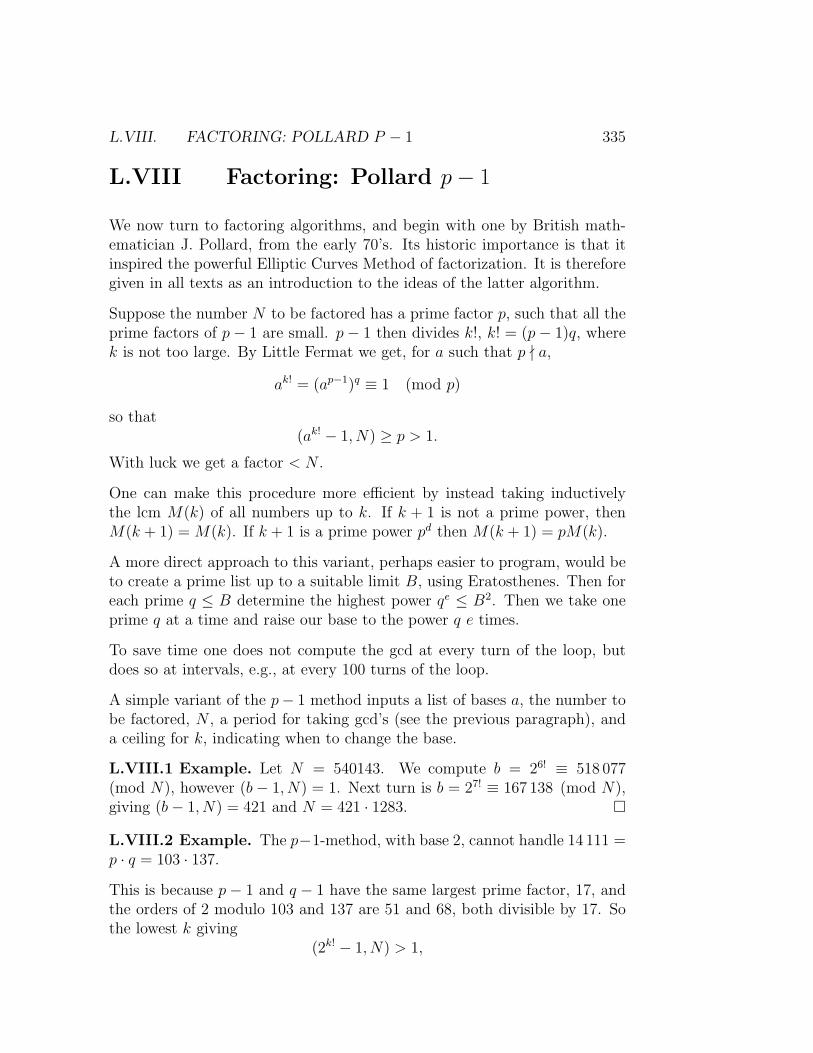
L.VIII. FACTORING: POLLARD P − 1 335
L.VIII Factoring: Pollard p− 1
We now turn to factoring algorithms, and begin with one by British math-ematician J. Pollard, from the early 70’s. Its historic importance is that itinspired the powerful Elliptic Curves Method of factorization. It is thereforegiven in all texts as an introduction to the ideas of the latter algorithm.
Suppose the number N to be factored has a prime factor p, such that all theprime factors of p− 1 are small. p− 1 then divides k!, k! = (p− 1)q, wherek is not too large. By Little Fermat we get, for a such that p - a,
ak! = (ap−1)q ≡ 1 (mod p)
so that(ak! − 1, N) ≥ p > 1.
With luck we get a factor < N .
One can make this procedure more efficient by instead taking inductivelythe lcm M(k) of all numbers up to k. If k + 1 is not a prime power, thenM(k + 1) = M(k). If k + 1 is a prime power pd then M(k + 1) = pM(k).
A more direct approach to this variant, perhaps easier to program, would beto create a prime list up to a suitable limit B, using Eratosthenes. Then foreach prime q ≤ B determine the highest power qe ≤ B2. Then we take oneprime q at a time and raise our base to the power q e times.
To save time one does not compute the gcd at every turn of the loop, butdoes so at intervals, e.g., at every 100 turns of the loop.
A simple variant of the p− 1 method inputs a list of bases a, the number tobe factored, N , a period for taking gcd’s (see the previous paragraph), anda ceiling for k, indicating when to change the base.
L.VIII.1 Example. Let N = 540143. We compute b = 26! ≡ 518 077(mod N), however (b− 1, N) = 1. Next turn is b = 27! ≡ 167 138 (mod N),giving (b− 1, N) = 421 and N = 421 · 1283. �
L.VIII.2 Example. The p−1-method, with base 2, cannot handle 14 111 =p · q = 103 · 137.
This is because p− 1 and q − 1 have the same largest prime factor, 17, andthe orders of 2 modulo 103 and 137 are 51 and 68, both divisible by 17. Sothe lowest k giving
(2k! − 1, N) > 1,

336 CHAPTER L. PRIMALITY AND FACTORIZATION
is k = 17. And thenN |2k! − 1,
as both 51 and 68 divide 17!.
The probability for something similar happening for large N is negligible.Also, really small factors should be found by trial-division before attemptinganything else. �
L.VIII.3 Example. Factoring
N = 83910 72126 67598 13859 = 45456 46757 · 1 84595 78087,
using the base 2, and a gcd-period of 100, takes little more than a second onmy machine, in fact much less, when using the lcm approach. This is becauseone of the prime factors minus one has small prime factors:
45456 46757− 1 = 22 · 7 · 8837 · 18371.
N = 31 61907 57417 40159 = 806 008 537 ·39 229 207 takes longer. Here is thereason:
806 008 537− 1 = 2 · 3 · 3 731 521,
39 229 207− 1 = 2 · 3 · 6 538 201.
Using the naive k! approach is at least ten times slower than using a primelist as indicated above.
There are further improvements (“phase two”, “stage two”) see, e.g., Crandall-Pomerance. Without these refinements, the Pollard rho algorithm, to bepresented below, usually wins. �
L.IX Factoring, Pollard rho
The rho method, another invention of Pollard’s, is very easy to program. Itdoes not depend on exponentiations, but does require Euclid. Each turn ofthe loop requires three polynomial evaluations, and half of the values arecomputed twice, a waste we can live with. Richard Brent has proposed avariant avoiding this, see the end of this Section.
N is the number we want to factor. The number p is an unknown prime fac-tor, e.g., the smallest one. We already know, by a Miller-Rabin test (SectionL.VI), that N is composite.

L.IX. FACTORING, POLLARD RHO 337
We try to create a sequence of numbers x0, x1, x2, . . . which appears to ex-hibit a random distribution modulo N , such that eventually two of them arecongruent modulo p. One does this by repeated application of a simple poly-nomial function f – often f(X) = X2 + c, c 6= 0,−2, or f(X) = X2 +X + 1will do the trick. The optimal number of iterations is some moderate multipleof N1/4, which we set as the ceiling for the number of turns of the loop.
We then choose some x0 and form x0, x1 = f(x0), x2 = f(x1), . . .
If xj − xi ≡ 0 (mod p) then also f(xj) − f(xi) ≡ 0 (mod p). Therefore itseems reasonable to form x2k − xk so that the distance keeps increasing. Sowe work with the two sequences xk, yk = x2k in parallel, which means threeevaluations for each iteration, as the y-sequence is updated twice.
In our quest for factors, at each turn of the loop we compute the gcd d =(x2k−xk, N) and output d,N/d if i d 6= 1, N (and then Miller-Rabin-test thefactors and continue). If we do not achieve a factorization before hitting theceiling we repeat with a different function. A recursive program (starting bytrialdividing out all factors below, say, 104) will handle at least any 30-digitnumber in a few minutes, with reasonable confidence. The worst case is anumber composed of two primes of similar size.
This particular iteration scheme is due to the American computer scientistRobert Floyd (1936-2001).
L.IX.1 Example. N = 540143.
Using f(x) = x2 + 1 and x0 = y0 = 1 we get
x1 = 2, y1 = 5, (5− 2, N) = 1
x2 = 5, y2 = 677, (677− 5, N) = 1
x3 = 26, y3 = 455 057, (455 057− 26, N) = 1
. . .
x24 = 26 630, y24 = 174 822, y24 − x24 = 148 192, (148 192, N) = 421.
�
One should not take gcd’s at every turn of the loop. Better to assign aperiod and multiply that number of differences (modulo N , of course) beforetaking the gcd. In order not to miss small factors, we trial-divide as alreadymentioned.
The optimal period would depend on the expected number of iterations.Already a period of 100 makes the time spent on Euclid relatively negligible.

338 CHAPTER L. PRIMALITY AND FACTORIZATION
L.IX.2 Example. In the Sections on trial division and Pollard p−1 we stud-ied the factorization of the number N = 31 61907 57417 40159 = 39 229 207 ·806 008 537, Using f(X) = X2 +X + 1, x0 = 1, gives a factorization withina fraction of a second. Taking gcd’s at intervals of 100 speeds things up bya factor 10.
Using f(X) = X2 + 1, x0 = 1, is about 8 times as slow. The performancemay vary greatly and unpredictably with the choice of the iterating functionf . �
The expected number of iterations lies somewhere around a moderate multi-ple of the square root of the smallest prime factor, assuming random behavior.
Suppose we randomly pick one out of p objects numbered 0, 1, . . . , p− 1. (Inour application the objects are the classes modulo the smallest prime factorp.) Suppose we do so m times, repeats allowed.
For each j, 0 ≤ j ≤ p − 1, we let Xj denote the stochastic variable definedby Xj = 1 if the j:th element is picked at least once, Xj = 0 otherwise.
Consider the sumX = X0 +X1 + · · ·+Xp−1.
X = k if k different objects are picked. The expected number q(m, p) ofdifferent outcomes on m trials therefore equals the expected value of X.
The expectation of any Xj obviously equals the probability that element jis picked. The probability that it is not picked is (1− 1/p)m, the probabilitythat it is picked therefore equals 1−(1−1/p)m. From this we see, by summingthe expectations, that
q(m, p) = p ·(
1− (1− 1
p)m
).
Applying Taylor’s Theorem to f(x) = (1 + x)m gives
f(x) = 1 +mx+m(m− 1)
2x2 + error
where the absolute value of the error term is less than m(m−1)(m−2)|x|3/6.
Substituting x = −1/p we obtain the following approximation for q(m, p) :
q(m, p) = m− m(m− 1)
2p+ error

L.IX. FACTORING, POLLARD RHO 339
with error term less than m(m− 1)(m− 2)/(6p2). So q(m, p) is less than mby a couple of units if m is a small multiple of
√p, in other words, for such
a choice of m the expected number of repeats is positive.
More on this topic, with explicit calculations of probabilities can be found inelementary textbooks on probability, under the heading “birthday paradox”.
Brent’s Modification
We give here a modified approach by Australian mathematician R Brent(1946-). Let the iterates be xm, yn. We update m,n and x, y according tothe following scheme:
(m,n) =(1,2)
(2,4)
(4, 7), (4,8)
(8, 13), (8, 14), (8, 15), (8,16)
(16, 25), (16, 26), (16, 27), (16, 28), (16, 29), (16, 30), (16, 31), (16,32)
. . .
The number of pairs in each row is a power of 2. Note how the index differenceincreases by one unit in each step, and only y is iterated on. Try to see thewhole of the pattern before reading further.
One could program this scheme as follows. Initialize m = 1, n = 2, andthe iterates x = x1 (input value) and y = x2 = f(x1). Suppose we havereached (m,n) = (2k−1, 2k), x = xm, y = yn. We then put r = n, x = y, n =m + n + 1, and y is iterated on m + 1 times. Then put m = r, and iterateon y, update n, until n = 2 ·m = 2k+1. Simultaneously form the differencesx−y and multiply them to the product. Take gcd’s at intervals, as indicatedabove.
Clearly higher iterates will be formed than with the Floyd method, but therewill be fewer evaluations, about 2/3 as many. The actual gain in speed isabout 20 − 25%. Riesel’s book discusses the mathematics involved in thisestimate, at least for f(X) = X2 + a.
L.IX.3 Example (A Pratt Certificate). Wishing once to factor the re-punit (1041 − 1)/9 completely, I trial divided to the limit 106 (again, weshould really combine this with some other factoring method) and Miller-

340 CHAPTER L. PRIMALITY AND FACTORIZATION
Rabin-tested (to several bases) the cofactor:
1041 − 1
9= 83 · 1231 · 53897 · 20176 37099 00322 80374 86579 42361.
Here the large cofactor N is a strongly suspected prime. We need to knowwith absolute certainty that it is prime. Hoping to expose it with Pockling-ton’s method (L.VII.3) I tried to factor N−1, again trialdividing to the limit106, and Miller-Rabin-testing the cofactor:
N − 1 = 23 · 3 · 5 · 11 · 41 · 9661 · 3 85889 69828 15807 76323.
The cofactor M = 3 85889 69828 15807 76323 is again a strong suspect, andis subjected to the same procedure:
M − 1 = 2 · 13 · 947 · 15 67255 69929 97351.
This time a Miller-Rabin test shows that the large cofactor
L = 15 67255 69929 97351
is composite. Pollard rho finds the factors L = 271 58563 ·5770 76077. Thesefactors are so small that full trial division will expose their primality. Ifinstead we stick to trialdividing only up to 106, we find 271 58562 = 2 ·32 ·19 ·79411 and 5770 76077−1 = 22 ·34 ·17 81099, with 1781099−1 = 2·11·19·4261.
I could now work from the bottom up, verifying the primality of1718099, 577076077, 27158563, L, M, and, finally, N , using Pocklington. Ob-viously this test lends itself splendidly to recursive programming.
Note that one need not really use all prime factors of N − 1. For instance,we can always exclude the factor 2.
In our example, the smallest base b for which
(b(N−1)/2 − 1, N) = 1
is 19 (a primitive root, in fact), and we do not need that step at all.
One could of course work with the factors of N −1 in descending order, untiltheir product exceeds
√N . Problems arise, of course, when the second largest
prime factor is so large that we cannot even achieve a tentative factorization.
This certification scheme due to V. Pratt, combines equally well with thePrimitive Root Test. The primality proof achieved goes under the name ofPratt certificate. �

L.IX. FACTORING, POLLARD RHO 341
L.IX: Exercises
1. (H W Lenstra, J Pintz, W L Steiger, E Szemeredi). Prove the followingstatements.
(a) Suppose n is a positive integer satisfying n ≤ 33m. If there is a positiveinteger a such that
a3m ≡ 1 (mod n), (a3m−1 − 1, n) = 1,
then n is a prime or a product of two primes ≡ 1 (mod 3m).
(b) Suppose n = (x · 3m + 1)(y · 3m + 1) ≤ 33m and
n = A · 32m + B · 3m + 1, 0 < A < 3m, 0 < B ≤ 3m.
Then xy = A, x + y = B.
(c) Suppose n = A · 32m + B · 3m + 1, 0 < A < 3m, 0 < B ≤ 3m. Then nis a prime if and only if
i. there is a positive integer a such that
a3m ≡ 1 (mod n), (a3m−1 − 1, n) = 1,
andii. B2 − 4A is a square
Hint: (X − x)(X − y) = X2 − (x + y)X + xy.
2. Use the rho method with f(X) = X2 + 1 to factorize
(a) 36563 94819 17866 84703 into two factors, and
(b) 3245 64576 76789 98977 into three. Miller-Rabin-test the factors to sev-eral bases (if you have a program for complete trial division, you canuse that as a deterministic primality test.)
3. A more ambitious project would be to write a full recursive factoring pro-gram trialdividing out the factors below 105 or 104, then using rho to findfurther factors, returning a full set of Miller-Rabin-tested factors. Ideally,if running too long, it should output the factors it found, along with thecofactor, certified to be composite.
Your program should be able to handle
(a) 526 31814 39815 23188 28920 59893
(b) 12051351 · 296 + 1
(c) 2109 − 255 + 1

342 CHAPTER L. PRIMALITY AND FACTORIZATION
(d) (1037 − 1)/9
(e) (1047 − 1)/9
(f) 2136 + 1
(g) 593 + 1
(h) 34 56456 45675 75787 68689 79790 808113
(i) 3225 − 1 (This one will take some time, possibly 15 minutes).
4. The performance of the rho method varies greatly with the input. The sameholds for the p−1 method of the previous section, but, as indicated there, forother reasons. You may enjoy writing a similar program as in the previousexercise and testing the same numbers.
A number that p− 1, but not rho, will easily crack is 1053− 1. Find, and atleast Miller-Rabin-test, the factors. Then use that same program to explainthe success of the p− 1 method.
5. A natural continuation of the previous exercises would be to find Prattcertificates for the large factors.
6. You may also like to try the Fermat number F8 = 228+1 which was cracked
in 1980, by Brent and Pollard, using a somewhat special iteration function,x210
+ 1, and initial value x0 = 3. You can find the explanation in Riesel’sbook or in the original article, “Factorization of the Eighth Fermat Number”,Mathematics of Computation, Vol. 36, No. 154, (Apr., 1981), pp. 627-630.
Today, a standard rho routine will find two factors, P,Q (in about twicethe time). Surprisingly, even the larger factor Q (62 digits) can be Pratt-certified in “reasonable” time, a couple of minutes. The smaller factor Pcan (today) be certified by full trial division.
You may then be able to explain Brent and Pollard’s conclusion: “I amnow entirely persuaded to employ the method, a handy trick, on giganticcomposite numbers”.
Needless to say, perhaps, modern factorization routines and primality testscrack F8 in just a second or two. You should not try this exercise on a slowcomputer. If you wish to try F7 = 227
+ 1 you should definitely use thespecial iteration function f(x) = x29
+ 1, intitial value x0 = 3, which runsabout six times as fast as a standard iteration.
Brent-Pollard’s general idea was to use the iteration function xm + 1 if therequired prime factors were known to be congruent to 1 modulo m.
7. Further suggestions for computing:
(a) Find primitive roots for some of the primes p you have encountered.Their computation relies on fast exponentiation (Section L.V) and fac-toring p− 1.

L.IX. FACTORING, POLLARD RHO 343
(b) A possible extension then is computing Discrete Logarithms, using,preferably, Pohlig-Hellman plus rho, as described in Section C.VII.

344 CHAPTER L. PRIMALITY AND FACTORIZATION
L.X “Waiting For a Square”
We now look at the crudest algorithm using continued fractions. Expanding√N , using the QCF (Section H.I), leads to the following relations:
p2k −Nq2
k = (−1)k+1Qk+1,
where pk, qk are steadily increasing, and 0 < Qk+1 < 2√N .
For some even k + 1 it might occur that Qk+1 is a perfect square =R2, say.It then holds that N |(pk −R)(pk +R). With bad luck one factor is divisibleby N , otherwise one of the gcd’s (pk − R,N) and (pk + R,N) produces agenuine factor of N .
If we are unlucky we continue until we register success. Perhaps one shouldhave a ceiling for the number of iterations; some moderate multiple of N1/4
will usually do.
L.X.1 Example. We have tried trial division, Pollard p − 1, and Pollardrho on the number 31 61907 57417 40159. The method just described cracksthat number in less than 0.1 seconds, after 7294 iterations, using not muchmore than 20 lines of code.
The right member Qk+1 is 33 235 225 = 57652 = R2. The corresponding pk
(reduced modulo N of course) is 18 92398 34711 35378. And we get:
(pk +R,N) = 806 008 537,
(pk −R,N) = 39 229 207.
�
Note that only the pk, not the qk, need be computed. And one should perhapsreduce them to their least absolute value remainders.
The reasonable range for this method seems to be up to about 25 digits.
L.X.2 Example. Unlike our previous examples, the following,
N = 203 80237 72101 12418 68065 58119
= 14060 51123 · 20292 56729 · 714 284 357
has three prime factors. The rho method finds the factors about 10 times asfast as “wait for a square” (using a gcd-period of 100). The main gain is infinding the first factor.
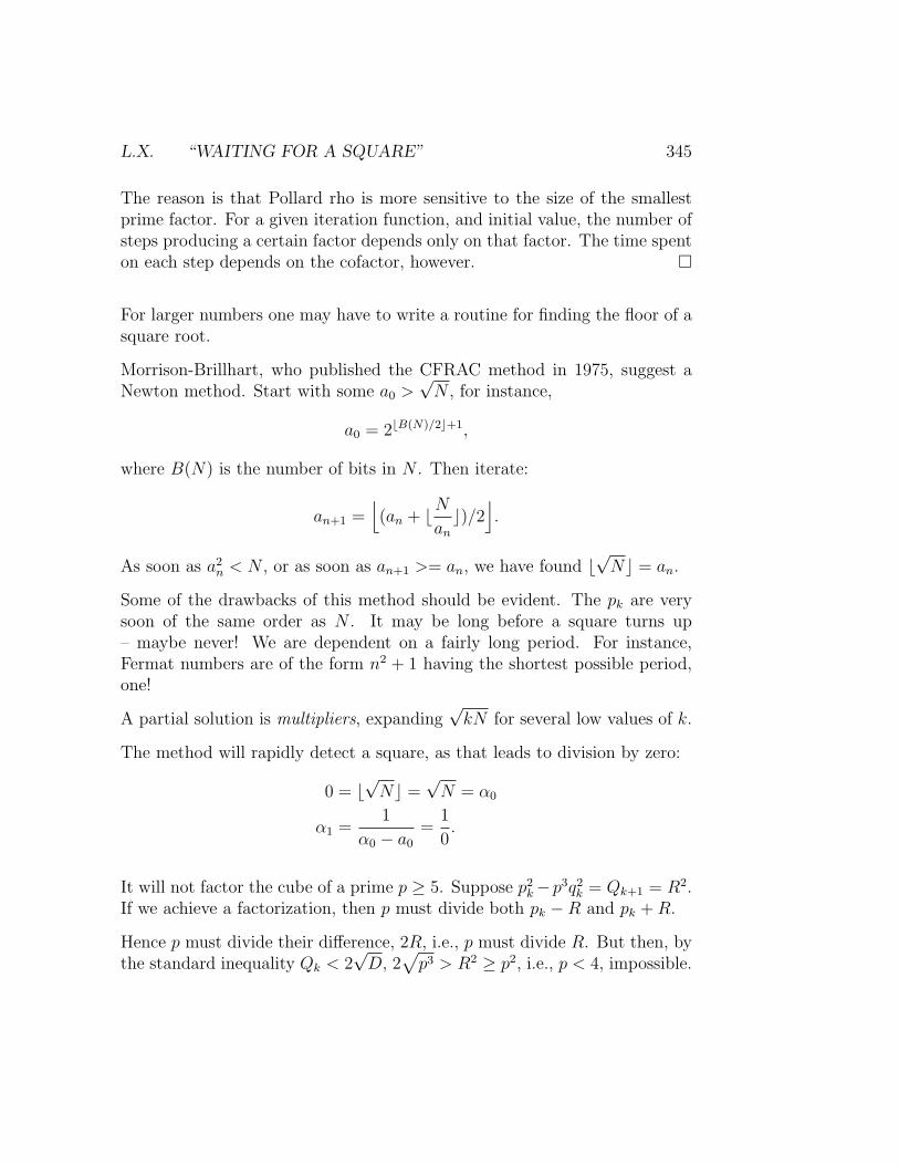
L.X. “WAITING FOR A SQUARE” 345
The reason is that Pollard rho is more sensitive to the size of the smallestprime factor. For a given iteration function, and initial value, the number ofsteps producing a certain factor depends only on that factor. The time spenton each step depends on the cofactor, however. �
For larger numbers one may have to write a routine for finding the floor of asquare root.
Morrison-Brillhart, who published the CFRAC method in 1975, suggest aNewton method. Start with some a0 >
√N , for instance,
a0 = 2bB(N)/2c+1,
where B(N) is the number of bits in N . Then iterate:
an+1 =⌊(an + bN
an
c)/2⌋.
As soon as a2n < N , or as soon as an+1 >= an, we have found b
√Nc = an.
Some of the drawbacks of this method should be evident. The pk are verysoon of the same order as N . It may be long before a square turns up– maybe never! We are dependent on a fairly long period. For instance,Fermat numbers are of the form n2 + 1 having the shortest possible period,one!
A partial solution is multipliers, expanding√kN for several low values of k.
The method will rapidly detect a square, as that leads to division by zero:
0 = b√Nc =
√N = α0
α1 =1
α0 − a0
=1
0.
It will not factor the cube of a prime p ≥ 5. Suppose p2k−p3q2
k = Qk+1 = R2.If we achieve a factorization, then p must divide both pk −R and pk +R.
Hence p must divide their difference, 2R, i.e., p must divide R. But then, bythe standard inequality Qk < 2
√D, 2
√p3 > R2 ≥ p2, i.e., p < 4, impossible.

346 CHAPTER L. PRIMALITY AND FACTORIZATION
L.X: Exercises
1. If you have already written a QCF routine, use “Wait for a Square” to factorthe numbers
(a) 36563 94819 17866 84703
(b) 5038 40507 49619 52087 41373
(c) 35419 05253 35205 94597 94529
(On the last number, Pollard rho will be much slower).
You should at least Miller-Rabin-test the factors. However, they are so smallthat full trial division will expose their primality in reasonable time.

L.XI. CFRAC 347
L.XI CFRAC
The idea behind CFRAC, published in the early 70’s, is one does not waitfor squares, one creates them.
We start by creating a list of primes, by Eratosthenes. We have checked thatthe number to be factored, N is composite, after extracting small factors,using trial division and/or the Pollard methods. N is odd, of course.
Note that p2k − Nq2
k = (−1)k+1Qk+1, (pk, qk) = 1; so if p is an odd primefactor of Qk+1, we must have (N/p) = 1. We therefore throw out all the oddprimes for which N is not a quadratic residue. We augment the list by thesign −1.
Then we run QCF. Each (−1)k+1Qk+1, k odd or even, is trialdivided againstthe factor base. If (−1)k+1Qk+1 factors completely, the exponents (takenmodulo 2) are stored in one list each, for every successful Qk+1. The exponentof −1 will be 1, if k is even, 0, if k is odd. At the same time the Qk+1 andpk are listed.
By Gaussian elimination mod 2 (to be explained in Section L.XII) we find acomplete set of independent relations modulo 2 among the exponent vectors.For each relation we multiply those (−1)k+1Qk+1 whose exponent vectorsenter the relation with coefficient 1. The product of these will be a square.At the same time we multiply the corresponding pk.
We call the resulting products Q = R2, and p. Multiplying the relations
p2k −Nq2
k = (−1)k+1Qk+1, p2k ≡ (−1)k+1Qk+1
shows thatp2 ≡ R2 (mod N),
and one can only hope that (p+R,N) or (p−R,N) produces a non-trivialfactor of N (it suffices to study one of them).
This method was first used with success by Brillhart and Morrison, in 1970,to factor F7 = 2128 +1, a 39-digit number. They used a multiplier, 257, aftersome experimentation, to get a reasonably long period, and an optimal factorbase. The factorization took several hours. Note that, unlike Pollard rho,the CFRAC method is insensitive to the size of the smallest prime factor.
The prime factorization of F7 is
59 64958 91274 97217 · 57 04689 20068 51290 54721.

348 CHAPTER L. PRIMALITY AND FACTORIZATION
A modern algorithm, run on a modern computer, finds the factors in lessthan a second.
There are a number of refinements.
One is “early abort”. The bigger the factor base, the more Qk’s factor overit. However, expanding the factor base also means that many unsuccessfulfactoring attempts last longer. The strategy then is to interrupt trial divisionsthat seem to last too long. At one or two cuts of the factor base one checkswhether the unfactored portion of Qk exceeds a prescribed fraction of 2
√N .
If so, the factoring process is interrupted and the next Qk is examined.
Another is “large prime variation” . If a number fails to factor completelyover the factor base, the remaining factor R is seen to be a prime number ifit is less than the square p2
max of the last prime of the factor base.
It is then saved. If Qk and Ql, l > k, have R as their largest prime divisor,then QkQl/R
2 factors over the factor base. At the same time we have tomatch this with pkpl ·R−1 (mod N).
(One will actually have to lower the limit quite a bit below p2max, to increase
the frequency of repeats. A moderate multiple kpmax, say 100 ≤ k ≤ 200,seems to work well).
If m > 1 different Qk contain the same large prime factor R, then m − 1factorizations are created.
The inversion and division step in the next to last paragraph, although oftenindicated in the literature, is not really needed.
Fix the first Qk having the large prime factor R. Consider each succeedingQl having that same large prime factor R. Q′
l = QkQl is then of the formQ′′
lR2 where Q′′
l factors over the factor base. Knowing the exponent vectors ofQk, Ql (ignoring the large prime factor R) we add these to get the exponentvector of Q′′
l
We then find the relations between the exponent vectors of the Q’s afterreplacing each of the Ql by Q′′
l .
Finally , for each relation (modulo 2) between the exponent vectors, multiplythe Q’s entering the relation, with each of the Ql replaced by Q′
l, and extractthe square root of that product (which is a perfect square, by construction).That can be done using an algorithm by Brillhart and Morrison to be pre-sented later. In this procedure we can determining the exponents modulo 2right away when trial dividing, at the cost of having to keep the Q’s.

L.XI. CFRAC 349
An alternative is to sum the corresponding nonreduced exponent vectors andhalve the sum, much as in the Example below.
The result is then matched against the product of the p’s with each pl replacedby pkpl. This variant appears to be slower.
Including a large prime variation in a CFRAC program requires a great dealof extra programming effort, including a sort. One stores triples consistingof Qk, preceded by their factor lists (headed by the large prime or 1), andthe corresponding pk. The triples are sorted, and collisions of first elements> 1 (the large prime) are handled as indicated above.
More details can be found in Riesel.
Finally, there are faster alternatives to the standard Gaussian algorithm fordetermining the dependencies, requiring, however, a much greater program-ming effort. These are of even greater importance in the more modern algo-rithms, such as the Quadratic and Number Field Sieves.
Without any of these refinements the reasonable range for using CFRAC(as a pastime) seems to be up to 35 digits. It has been supplanted by theQuadratic Sieve.
L.XI.1 Example. We illustrate a simple variant of the method on N =12007001 (cf. the discussion in Riesel’s book). Like most didactical examplesit is really too small to illustrate the advantages of CFRAC over, e.g., trialdivision.
We use a factor base of nine elements, -1, and the eight smallest primes suchthat (N/p) = 1. The base is
−1, 2, 5, 23, 31, 43, 53, 59, 61.
We run QCF and make lists of the 10 first k, pk, (−1)k+1Qk+1, such that(−1)k+1Qk+1 factors completely over the factor base. The pk are reduced

350 CHAPTER L. PRIMALITY AND FACTORIZATION
modulo N. We arrive at the following table:
k pk ±Qk+1
5 2 228 067 409 668 093 1475
17 20 40020 10 806 646 −97623 7 209 052 236026 11 477 859 −15527 6 764 708 204829 10 273 669 400031 4 333 614 189132 7 018 490 −2440
The matrix of exponent vectors, written as a list of lists, is
[[0, 3, 1, 0, 0, 0, 0, 0, 0],
[0, 0, 2, 0, 0, 0, 0, 1, 0],
[0, 4, 2, 0, 0, 0, 0, 0, 0],
[1, 4, 0, 0, 0, 0, 0, 0, 1],
[0, 3, 1, 0, 0, 0, 0, 1, 0],
[1, 0, 1, 0, 1, 0, 0, 0, 0],
[0, 11, 0, 0, 0, 0, 0, 0, 0],
[0, 5, 3, 0, 0, 0, 0, 0, 0],
[0, 0, 0, 0, 1, 0, 0, 0, 1],
[1, 3, 1, 0, 0, 0, 0, 0, 1]]
For instance, −976 = (−1) ·24 ·61, accounting for the fourth row. The matrixis typically sparse.
Gaussian elimination produces the following five (not just one!) linear rela-tions (modulo 2) among the exponent vectors:
[[0, 0, 1, 0, 0, 0, 0, 0, 0, 0],
[1, 1, 0, 0, 1, 0, 0, 0, 0, 0],
[1, 0, 0, 0, 0, 0, 0, 1, 0, 0],
[1, 0, 0, 1, 0, 1, 1, 0, 1, 0],
[1, 0, 0, 1, 0, 0, 0, 0, 0, 1]]

L.XI. CFRAC 351
The single 1 in the first relation reflects the fact that the correspondingQ = 400 is a square.
Let us have a closer look at the fourth relation. Numbering from 0 to 9,it expresses that the product of number 0,3,5,6,8 of the ±Q above is aperfect square. Indeed, the sum of the corresponding exponent vectors is[2, 18, 2, 0, 2, 0, 0, 0, 2] with all exponents even. Halving them gives
[1, 9, 1, 0, 1, 0, 0, 1].
Ignoring the sign (the first component) we see that Q = R2 where R =29 · 5 · 31 · 61 = 4840960.
The product of the corresponding pk is
p ≡ 2 228 067·10 806 646·11 477 859·6 764 708·4 333 614 ≡ 10 842 960 (mod N).
A little bit of Euclid then yields the (prime) factors
(p±R,N) = 3001, 4001,
and, indeed, N = 3001 · 4001.
The other four relations turn out to lead to only the trivial factors, on takingthe gcd’s.
We are still in the range where wait-for-a-square is faster (trial division isfaster yet). The first square Q2k is Q68 = 1024 = 322 and the correspondingp67 is ≡ 11 238 777 (mod N), and (11 238 777− 32, N) = 3001, (11 238 777 +32, N) = 4001.
The period of√N , should you wonder, is 870. �
L.XI.2 Example. We sketch here Brillhart-Morrison’s alternative methodfor finding the (modular) square root of a product, known to be a square. Itis useful also in the context of the Quadratic Sieve.
Suppose the product is Q1Q2 · · ·Qn. Suppose, for k < n, we have achievedthe factorization Q1Q2 · · ·Qk = d1d2 · · · dke
2 where di|Qi, i = 1, 2, . . . k andare relatively prime in pairs (initially, Q1 = Q1 · 1).
We store r = d1d2 · · · dk, the “reduced product”, and e, the “free factor”(reduced modulo N). We find the gcd, g = (r,Qk+1).
g contributes the factor g2 to the total product, and is therefore multipliedto the free factor. It has the form g = d′′1d
′′2 · · · d′′k, where d′′i divides di;
di = d′id′′i , i = 1, 2, . . . k.

352 CHAPTER L. PRIMALITY AND FACTORIZATION
The quotient dk+1 = Qk+1/g is relatively prime to r/g, which now has theform d′1d
′2 · · · d′k. We have achieved
Q1Q2 · · ·Qk+1 = (d′1d′2 · · · d′k · dk+1)(ge)
2
where the factor in the first pair of parentheses is our new reduced product,and the product ge is our new free factor (to be reduced modulo N).
When k + 1 = n, the reduced product must itself be a a square, since thewhole product is, by assumption, The final step is to multiply its square rootto the free factor, modulo N .
In the Example above, the factors are 40, 976, 155, 2048, 1891. The first gcdis (40, 976) = 8, giving our first reduced product = 5 · 122 = 610, and freefactor = 8.
Next, (610, 155) = 5, so our new reduced product is (610/5) ·(155/5) = 3782,and the new free factor is 5 · 8 = 40.
We now look at the fourth factor, 2048. This time we get (3782, 2048) = 2,new reduced product 1891 · 1024 = 1936384, and free factor 2 · 40 = 80.
The last factor is 1891, (1 936 384, 1 891) = 1 891, giving the reduced product1 936 384/1891 = 1024 and free factor 1891 · 80 = 151280. 1024 = 322 so thedesired square root is 32 · 151 280 = 4 840 960.
�
L.XI.3 Example. The following example
N = 6589 68977 39494 03132 93285 74193 88201
has 34 digits. The factorization is
N = 474 64739 77078 59989 · 13 88333 69903 04709.
Using a very simple program, and a factor base of 300 primes, led to 21relations, (the typical proportion seems to be 5-10% of the length of thefactor base).
Typically (for the case of two prime divisors), about half of them, 11 to beexact, led to factorizations. For, e.g., three primes, a greater portion factors,and generally, any factorization will occur.
The whole process took me 267 seconds, 0.12 of which were spent on rowreduction. In the example above, I also tried a smaller base, of 200 primes,

L.XI. CFRAC 353
looking for 200+a few extra factorizations (the extras are usually not neces-sary, the system will be singular anyway).
That choice cut the running time by 50 seconds. A simple early abort stategy,stopping at the 50th prime, if the unfactored portion exceeded 2
√N/100, cut
the time by another 75 seconds.
I have also tried a crude large prime variant, with a factor base of 100 primesbringing the running time down to 80 seconds.
A more sophisticated program combines the two tricks. With the same basis,moving the cut down to 15th prime, and lowering the limit for the unfactoredportion to 2
√N/500, I brought the running time down to 40 seconds (for
larger numbers, the divisor 1000 seems more appropriate). Introducing cutsat the 10th and 30th primes, with divisors 500 and 105 brought the runningtime down to 20 seconds. Clearly, early aborts produce great effects giventhe scant extra programming effort.
My method of dealing with the large primes was to set a negative numberof extras, extra= −k · L, where k lies somewhere between 0.4 and 0.6. Thedesirable number of factorizations was set to L+extra. The large primelimit was set at 200 times the largest prime in the factor base, and shouldpossibly be set lower for a number this size. Each time a large prime wasdetected the variable extra, hence also the target number of factorizations,was augmented by one. The number of large primes in this case was around1000, and there were about 75 repeats, yielding enough factorizations.
Denoting by FF the number of full factorizations over the factor base, andFL the number of factorizations including a large prime, a more orthodoxprocedure is to go on factoring until FF + k · FL exceeds the size of thefactor base. k is a constant < 1, something like 0.6− 0.7 will do.
The number 257 ·F7 = 257 · (2128 + 1) is a historically interesting example asit was first cracked using CFRAC (the multiplier 257, found by experimen-tation, was introduced in order to achieve a reasonably long period).
Using a base of 200 primes and large prime variation with −120 “extras”,my program ran for about 15 minutes, a 50% improvement over the basicalgorithm.
An early abort at the 15th prime, with divisor 1000 took 5 minutes off that.A second cut, at the 50th prime, with divisor 106, produced an even moredrastic reduction, to less than 4 minutes.

354 CHAPTER L. PRIMALITY AND FACTORIZATION
Keeping the first divisor, raising the second one to 4 · 107, and moving thecuts back to positions 10 and 30, reduced the running time even further, to138 seconds. I have not made any further experiments on numbers of thissize.
S Wagstaff and C Pomerance experimented a lot with these parameters inthe 80’s, but with much larger numbers and on a base of 959 primes. Theyrecommended a second cut at the 95th prime, with divisor 4 · 107.
These running times are not very impressive in comparison with newer meth-ods. There are more devices for speeding up a CFRAC program. However,given the greater efficiency of the newer methods, it is doubtful whetheranyone would like to spend his energy on such efforts. Already a single-polynomial Quadratic Sieve, without large prime variation, is as fast, or evenfaster than CFRAC when we go beyond 35 digits.
A simple Elliptic Curves program of mine, comprising maybe 120 lines ofcode, cracks F7 in a second. That method , like Pollard rho, is sensitive tothe size of the smallest prime factor, which in this case has 17 decimal digits.
CFRAC was developed and implemented by Brillhart and Morrison in 1970.Their original article, “A Method of Factoring and the Factorization of F7”was published in Mathematics of Computation, Vol. 29, No. 129, Jan., 1975,pp. 183-205, and is yet today a very delightful and historically interestingread.
�
L.XII Elimination Modulo 2
Here we exemplify a standard algorithm for Gaussian elimination modulo 2.
We want to determine the dependencies among the rows of the matrix
1 1 01 0 10 0 11 1 1
We want to eliminate from right to left. Therefore we augment the matrix

L.XII. ELIMINATION MODULO 2 355
by an identity matrix to the left :
1 0 0 0 1 1 00 1 0 0 1 0 10 0 1 0 0 0 10 0 0 1 1 1 1
From elementary Linear Algebra you will recall that the elimination processcreates zero rows to the right of the vertical line. The rows to the left of thezero rows will then give a complete set of linear relations among the the rows– they record the total row operation that produced the zero row.
“Complete” means every linear relation is a (unique) linear combination ofthese rows.
Looking at the last column we already have a zero in the first position. Inthe next position there is a one, and adding that row to the two rows belowit creates zeros in their places:
1 0 0 0 1 1 00 1 0 0 1 0 10 1 1 0 1 0 00 1 0 1 0 1 0
We now delete the row we used, and the last column:
1 0 0 0 1 10 1 1 0 1 00 1 0 1 0 1
Next we add the first row to the third:
1 0 0 0 1 10 1 1 0 1 01 1 0 1 1 0
Again we delete the row we used, and the last column:
0 1 1 0 11 1 0 1 1
Finally we add the first row to the second:
0 1 1 0 11 0 1 1 0

356 CHAPTER L. PRIMALITY AND FACTORIZATION
Deleting the first row, and the last column now leaves us with the coefficientsof the relations between the four rows:
1 0 1 1
Each row in the matrix is a list (or whatever) of binary numbers that happento equal 0 or 1, with lots of zero bits. The procedure is made more efficientby converting the list of binary numbers to one number, or one string of bits,using the shift and “bitwise or” operators. In Python the construction mightlook like this:
def pack(v):
n=0L
for k in v:
n=(n<<1)|k
return n
where v is the list representing a row in the matrix. The shift, <<, representsmultiplication by 2, and the “or” operator (the vertical) adds in the bit k tothe last place of n.
It pays to work in blocks by shifting n to the left (n << 32) repeatedly andpacking segments of 32 elements of the list v. An alternative is to pack intoseveral 32-bit words, and do the elimination in blocks.
The list of the four given rows will look like this on the screen, in decimalnotation:
[6, 5, 1, 7].
Augmenting to the left with an identity matrix will look like adding 64 =26, 32 = 25, 16, 8 to these numbers. The 2-powers are represented by leftshifts of 1. The additions again are “bitwise or” operators.
The additions modulo 2 used in creating zeros are bitwise exclusive-or oper-ators. Deletion of a zero column is division by two, represented by a shiftoperator (the routine can be arranged so as to save these shifts for last).
The “unpacking” is executed by “bitwise and” and shifts. In Python it mightlook like:
def unpack(n):
v=[]
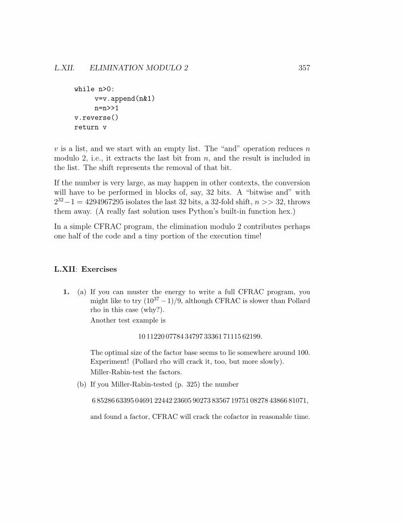
L.XII. ELIMINATION MODULO 2 357
while n>0:
v=v.append(n&1)
n=n>>1
v.reverse()
return v
v is a list, and we start with an empty list. The “and” operation reduces nmodulo 2, i.e., it extracts the last bit from n, and the result is included inthe list. The shift represents the removal of that bit.
If the number is very large, as may happen in other contexts, the conversionwill have to be performed in blocks of, say, 32 bits. A “bitwise and” with232−1 = 4294967295 isolates the last 32 bits, a 32-fold shift, n >> 32, throwsthem away. (A really fast solution uses Python’s built-in function hex.)
In a simple CFRAC program, the elimination modulo 2 contributes perhapsone half of the code and a tiny portion of the execution time!
L.XII: Exercises
1. (a) If you can muster the energy to write a full CFRAC program, youmight like to try (1037− 1)/9, although CFRAC is slower than Pollardrho in this case (why?).Another test example is
10 11220 07784 34797 33361 71115 62199.
The optimal size of the factor base seems to lie somewhere around 100.Experiment! (Pollard rho will crack it, too, but more slowly).Miller-Rabin-test the factors.
(b) If you Miller-Rabin-tested (p. 325) the number
6 85286 63395 04691 22442 23605 90273 83567 19751 08278 43866 81071,
and found a factor, CFRAC will crack the cofactor in reasonable time.

358 CHAPTER L. PRIMALITY AND FACTORIZATION
L.XIII Quadratic Sieve
Orientation
The most important modern factoring algorithms are the Elliptic CurvesMethod (ECM), the Multiple Polynomial Quadratic Sieve (MPQS), and theNumber Field Sieve (NFS). Of these the first and the third depend on exten-sive theoretical preparations beyond the scope of this text. The QuadraticSieve is very elementary in comparison. The analysis of its performance isless elementary, of course.
NFS is responsible for some recent spectacular factoring records, althoughits practicality has been questioned. ECM is best suited for finding primefactors of 20-30 digits, even in very large numbers. It is remarkable in itsminimal storage requirements and the modest programming effort that goesinto it.
As an introduction to the full Quadratic Sieve algorithm, as described in,e.g., Crandall-Pomerance, I will first outline a simple version of the singlepolynomial Quadratic Sieve. Even in this simple form, requiring a few pagesof code, the QS outdoes CFRAC (even with large prime variation and earlyaborts) at least from 35 digits upwards. It is not nearly as fast as the MPQSor ECM, but it will crack 40-digit numbers while you check your email and45-digit numbers while you prepare a meal.
The number we wish to factor is denoted N . It is odd and has been provencomposite. By trivial division (up to, say, 5 · 105 ) and, e.g., a standard rhoroutine (with, say, 106 turns of the loop) we have removed all smaller factors,perhaps up to 10 digits. A more serious program would remove even largerfactors, using the ECM.
We let m denote the floor of√N . We will use a sieving polynomial f(X) =
(X+m)2−N . We are looking for X-values in a symmetric interval |X| ≤M ,M much smaller than m (the sieving interval), for which f(X) factors over afactor base. Such a base consists of the sign −1 and prime numbers p belowa prescribed smoothness bound B. Of these we need only keep the prime 2(if N ≡ 1 (mod 8)) and those odd p for which (N/p) = 1, of course.
The factorizations determine exponent vectors modulo 2. By Gaussian elim-ination we can find combinations of vectors that sum to zero modulo 2.Multiplying the corresponding polynomial values f(X) on the one hand, andthe corresponding (X +m)2 on the other hand, we arrive at congruences of

L.XIII. QUADRATIC SIEVE 359
the form a2 ≡ b2 (mod N). Hopefully one or both of the gcd’s (a± b,N) willthen reveal a proper factor of N .
The product a of the X +m modulo N is easy to determine if we store the(X + m)-values in a list as we go along. Storing the corresponding f(X)-values, and using Brillhart–Morrison’s algorithm, we find the value for b.
We cannot afford to trial-divide all the values of f(X) over the factor base.We must have some crude method of selection of the X to try.
The basic idea, soon to be modified, is the following. For each prime p thereare two square-roots of N modulo p. Let us call them ±r. For each numberof the form X = k · p± r in the sieving interval the prime number p dividesf(X). If we start with a list of ones we could multiply in those factors p intheir respective locations. Doing this for all p, we would find which f(X)factor completely.
There is however one error and several flaws in this procedure. We areforgetting multiple factors – small primes frequently are. For instance, ifN ≡ 1 (mod 8), half of the values are divisible by 8. Sieving over smallprimes is also very time-consuming. It is furthermore too time-consumingto compute all the polynomial values. The modified idea is to first find outwhich polynomial values are reasonably close to factoring, and only thenperform the trial division.
In dealing with approximations we also replace multiplication by the fasteroperation addition, i.e., we work with (approximate) logarithms, e.g., theintegers closest to the various 2-logarithms. I found it expedient to excludeseveral small primes, when sieving.
Also we do not check whether the logarithms, in the location correspondingtoX, sum approximately to log(|f(X)|). Instead we choose a constant target,the log of the average of |f(X)|. As m2 approximates N , and X2 is smallcompared to N , |(X + m)2 − N | ≈ |2mX|, the average of which is mM .Our target is therefore taken as an approximation of log(m) + log(M) ≈log(N)/2 + log(M).
We will have to subtract a small error term d to compensate for the fact thatwe leave out small primes and ignore prime powers. In case we introduce thelarge prime variation, described in the context of CFRAC, a common choiceis to subtract d = 2 · pmax where pmax] is the largest prime of the factor base.
Those X that produce a sum of logarithms exceeding log(N)/2+ log(M)−dare those for which we trialdivide f(X) over the factor base. That saves a lot

360 CHAPTER L. PRIMALITY AND FACTORIZATION
of work. Only perhaps a few hundred values in a million are tested – or evencomputed! – and a substantial portion of these yield full factorizations. Thisportion will depend on details of the program, such as the choice of errorterm and the number of primes (or prime powers!) excluded from sieving.
With limited storage we are forced to work in blocks, i.e., we process intervalsof a given length L, from the center outwards: [0, L) [−L, 0), [L, 2L) . . . . Onmy machine the ideal seems to be L = 106.
The number of blocks need not be specified in the single polynomial version;we could check the accumulated number of exponent vectors after each blockand quit sieving as soon as it exceeds the size F of the factor base (in all myruns 0.97 ∗ F sufficed).
With large prime variation it is not quite that easy. We must attach someweight to the number of large prime factorizations as we did with the CFRAC,and go on sieving until the weighted sum exceeds the length of the factorbase (or slightly less). A suggestion of Silverman’s is to stop when FF +(1−R)FL > R· the length of the factor base, where R is slightly less than 1, sayR = 0.96. FF again denotes the number of fully factored polynomial values,FL the number of those values including one large prime outside the factorbase.
For 39 digits the expected number of blocks is maybe 100, for 49 digitsseveral thousand –working with multiple polynomials reduces the sievinginterval drastically. The smoothness bound could be 45 000-50 000 for 39-40 digits, maybe 110 000-120 000 for 45-46 digits. These bounds are againsmaller in the full multiple polynomial algorithm, and smaller yet with largeprime variation - which in this case requires more storage than in CFRAC.The elimination stage is also more of an issue in QS as the factor bases fornumbers of a given size are much larger.
If the quantities a + b, a − b, hence also a, b, have an odd prime factor incommon it must belong to the factor base. As we have already weeded outsmall factors this means that QS will never crack a prime power. If you get100 relations in the elimination step and none of them leads to a factorizationyou will know why. Should you enter a square (prime or not), your factorbase would be about twice the expected size. It would probably make someof your parameter choices far from optimal.
But a serious factoring program should check this pathology at the beginning.The Newton procedure we have explained earlier for finding the floor of asquare root, is easily modified to find exact square roots, cubic roots, etc.

L.XIII. QUADRATIC SIEVE 361
Multiple Polynomials
Anyone who has written a basic QS program will have noticed how the num-ber of fully factored reports diminish as we travel away from the origin.Peter Montgomery’s ingenious idea was to introduce several sieving polyno-mials of the form (aX + b)2 −N , and sieve each over a shorter interval. Bychoosing a, b so that a | (b2 −N), the polynomial can be written in the forma(aX2 + 2bX + c) = ag(X), i.e., all its values are divisible by a.
By a skillful choice of a we can achieve that the values of g(X) are on theaverage of the same magnitude as those of (X + m)2 − N , or even slightlysmaller. We assume 0 < b < a/2. Then the minimum of ag(X) is closeto X = 0, so we sieve over a symmetric interval, |X| ≤ M . The minimumvalue is −N . The greatest values are assumed at the endpoints, and areapproximately a2M2−N . It is reasonable to make these two equal in absolutevalue, i.e., a2M2 ≈ 2N, a ≈
√2N/M . The approximate maximum of |g(X)|
is N/a ≈M√N/√
2.
Classical MPQS now chooses a to be the square of a prime number q. b is thento be taken as a square root of N modulo q2, available by, e.g. Berlekamp(+Hensel), or the Lucas sequences to be introduced in the next Section. Thesquare rooting routine can be avoided by choosing q ≡ 3 (mod 4). In thatcase the solution to x2 ≡ b (mod q) is, as we have noted before, x ≡ ±b(q+1)/4
(mod q).
There are two roots between 0 and a and we can choose the one closest to0. q can be generated by the methods introduced earlier. Note that we neednot determine c = (b2 −N)/a.
The sieving proceeds much as in the single polynomial case, only we have tothe factor a into account when trial dividing. Also, the average of |g(X)| ismore like
√2NM/3. Note that the factor base is the same as in the single
polynomial case – we are looking for primes p that divide (aX + b)2 − N ,hence we still require that (N/p) = 1.
The most time-consuming step when initializing a new polynomial is to inverta modulo each prime p in the factor base (or at least those used in sieving)so as to determine the roots of ag(X) modulo p. The square roots of Nmodulo p are computed at the beginning of the program and reused whendetermining the roots of a new sieving polynomial.
The extra effort in expanding a single polynomial routine to one using mul-tiple polynomials is surprisingly small, especially in comparison with large

362 CHAPTER L. PRIMALITY AND FACTORIZATION
prime variation. One should attempt the former first, as it brings down thelength of the lists involved.
The‘self-intializing” QS, known as SIQS, chooses a to be the product ofseveral prime numbers in the factor base. If a is composed of 5 prime factors,say, there are 32 square roots b of N modulo a, but as ±b yield the samepolynomial values we keep only half of them. Nonetheless, that means thatwe need only one inversion step to produce the roots of 16 polynomials, whichis a considerable saving when factoring large numbers.
For very clear accounts of the details I refer to Bressoud and Crandall-Pomerance (the Quadratic Sieve is Pomerance’s invention). The latter bookalso explains SIQS.
A very full, practical, account of SIQS is Scott Contini’s MSc thesis, down-loadable from his website, http://www.crypto-world.com/Contini.html.
The QS originated with Pomerance. Multiple polynomials is Peter Mont-gomery’s idea. The classical reference is Robert D Silverman: “The Multi-ple Polynomial Quadratic Sieve”, Mathematics of Computation, 48, No 177(1987), 329-339.
A reader with experience in the C programming language might enjoy study-ing the code in http://www.friedspace.com/QS/ (by William Hart, 28pages) or http://www.boo.net/∼jasonp/qs.html (by Jason Papadoupolos,99 pages).
L.XIV Lucas Sequences and Primality
Some earlier methods have relied on factoring N − 1 easily. Maybe we donot get enough factors that way. Then perhaps N + 1 might prove moresuccessful. The tool is Lucas sequences. For more details on these, see thebooks by Riesel and Bressoud-Wagon.
We study the linear recurrence
Sn+2 − PSn+1 +QSn = 0; n ≥ 0; S0, S1 given.
P,Q are integers. A popular choice is P = Q = 5 or P = 1, Q = ±2,±3, . . .– the theoretical reason for this is explained in Bressoud-Wagon.
The sequence S0, S1, S2, . . . then also consists of integers, uniquely deter-mined by the conditions. We will consider the same sequence taken modulo
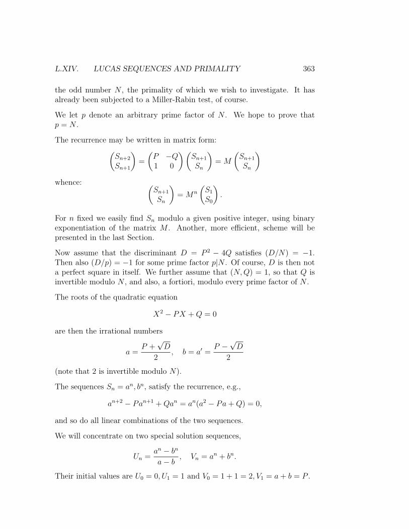
L.XIV. LUCAS SEQUENCES AND PRIMALITY 363
the odd number N , the primality of which we wish to investigate. It hasalready been subjected to a Miller-Rabin test, of course.
We let p denote an arbitrary prime factor of N . We hope to prove thatp = N .
The recurrence may be written in matrix form:(Sn+2
Sn+1
)=
(P −Q1 0
) (Sn+1
Sn
)= M
(Sn+1
Sn
)whence: (
Sn+1
Sn
)= Mn
(S1
S0
).
For n fixed we easily find Sn modulo a given positive integer, using binaryexponentiation of the matrix M . Another, more efficient, scheme will bepresented in the last Section.
Now assume that the discriminant D = P 2 − 4Q satisfies (D/N) = −1.Then also (D/p) = −1 for some prime factor p|N . Of course, D is then nota perfect square in itself. We further assume that (N,Q) = 1, so that Q isinvertible modulo N , and also, a fortiori, modulo every prime factor of N .
The roots of the quadratic equation
X2 − PX +Q = 0
are then the irrational numbers
a =P +
√D
2, b = a′ =
P −√D
2
(note that 2 is invertible modulo N).
The sequences Sn = an, bn, satisfy the recurrence, e.g.,
an+2 − Pan+1 +Qan = an(a2 − Pa+Q) = 0,
and so do all linear combinations of the two sequences.
We will concentrate on two special solution sequences,
Un =an − bn
a− b, Vn = an + bn.
Their initial values are U0 = 0, U1 = 1 and V0 = 1 + 1 = 2, V1 = a+ b = P .

364 CHAPTER L. PRIMALITY AND FACTORIZATION
From the identity
2(an+1 − bn+1) = (a+ b)(an − bn) + (a− b)(an + bn)
we conclude (dividing by a− b) that
2Un+1 = PUn + Vn.
Another useful formula is the doubling formula:
U2n = UnVn,
which follows directly from the conjugate rule
a2n − b2n = (an − bn)(an + bn),
again by division.
Now suppose Un ≡ 0, Un+1 ≡ m (mod N), where m is some integer. Thatis m times the initial values U0 ≡ 0, U1 ≡ 1 (mod N). This means thatthe sequence will repeat from n on, but multiplied by m. Hence also U2n =U3n = · · · = 0.
There is a shortest period k > 0 satisfying U0 = Uk = U2k = · · · = 0. Wenow prove that every other period is a multiple of k.
L.XIV.1 Lemma. Let M > 0 be a positive modulus, satisfying(Q,M) = 1. Let further k be the smallest positive index for whichUk ≡ 0 (mod M), and n > 0 an arbitrary index satisfying Un ≡ 0(mod M). Then k divides n.
Proof. We first note that if two irrationalities of the form r+ s√D, r, s ∈
Z, are (componentwise) divisible by M , then so is their product.
We next recall that ab = Q, so the invertibility of Q entails that of a and bmodulo M .
We then have the following equivalence:
Un ≡ 0 (mod M) ⇐⇒ an ≡ bn (mod M)
⇐⇒ a2n ≡ (ab)n = Qn (mod M),

L.XIV. LUCAS SEQUENCES AND PRIMALITY 365
where we get from the rightmost member to the middle member on multipli-cation by the the inverse to an modulo M . And from the first to the secondon multiplication by a− b =
√D.
Letting QR ≡ 1 (mod M), and multiplying the last congruence by Rn, weget
Un ≡ 0 (mod M) ⇐⇒ (a2R)n ≡ 1 (mod M).
k is by assumption the least n > 0 having that property. Hence it is the orderof a2R modulo M , and the Lemma follows by the general theory of orders ofinvertible classes, (A.V.5), readily generalizable to this case (exercise!). �
The number k is not the period of the sequence Un, properly speaking, onlyof the zeros appearing in it. Bressoud calls it the “rank” of the U -sequence.
Now consider the sequence taken modulo p, where p is a prime number suchthat (D/p) = −1. We will need to generalize Little Fermat. First we stateyet another version of “Freshman’s Dream”.
We let x and y denote integers or quadratic irrationalities of the form
c+ d√D,
where c = r/s, d = t/u are rational numbers, with r, u relatively prime top, hence invertible modulo p. Hence it is meaningful to speak of r/s, t/umodulo p. Then:
L.XIV.2 Lemma (Freshman’s Dream).
(x+ y)p ≡ xp + yp (mod p).
�
We are still assuming that D is not a quadratic residue modulo p, hencenot a perfect square. We will use the first part of the following Corollary toFreshman’s Dream. Applied to the situation above, and the two roots a, b,it implies ap ≡ b, bp ≡ a (mod p).
L.XIV.3 Corollary.(Dp
)= −1 ⇒ (c+ d
√D)p ≡ c− d
√D (mod p),

366 CHAPTER L. PRIMALITY AND FACTORIZATION
(Dp
)= 1 ⇒ (c+ d
√D)p ≡ c+ d
√D (mod p).
Proof.
(c+ d√D)p ≡ cp + dpD(p−1)/2
√D ≡ cp + dp
(Dp
)√D ≡ c+ d
(Dp
)√D
Here we used Euler’s Criterion and Little Fermat. �
With our previous notation, and the chosen p, it then holds that
Up ≡ap − bp
a− b≡ b− a
a− b≡ −1 (mod p),
and
Up+1 ≡ap+1 − bp+1
a− b
≡ a · b− b · aa− b
≡ 0 (mod p).
This shows that Uk ≡ 0 (mod p) occurs with period p+1 or a factor of p+1,if (D/p) = −1, and with period p− 1, or a factor of p− 1, otherwise.
So at least we have a pseudoprime test:
L.XIV.4 Theorem. Assumptions and notation as above. If
UN+1 6≡ 0 (mod N),
then N is composite.
L.XIV.5 Example. N = 450 74455 37641. With P = 1, Q = 3, D = −11,(D/N) = −1) one obtains UN+1 ≡ 72 44374 53394 6≡ 0 (mod N), and N iscomposite. It is a Carmichael number (cf. p. 90), N = pqr = 9091 · 18181 ·27271, with p− 1, q− 1, r− 1 dividing N − 1, resisting a simple Fermat test.(Note that the factors are of the form t+ 1, 2t+ 1, 3t+ 1.) �

L.XIV. LUCAS SEQUENCES AND PRIMALITY 367
One can prove the following sufficient condition for primality, in analogywith the Primitive Root test (L.VII.1):
L.XIV.6 Theorem. Assumptions as above. Suppose UN+1 ≡ 0(mod N), but U(N+1)/q 6≡ 0 (mod N) for each prime factor q|(N + 1).Then N is prime.
�
The proof depends on an investigation into the relevant analogue ofCarmichael’s λ function (C.V.3), the maximal order function ω(N). Onecan prove ω(N) ≤ 0.8N < N + 1 if N has at least two different primefactors.
In the case of of a prime power N = pt one proves that ω(N) divides pt±pt−1
(generally), and equals pt±1 (from the assumption). However, pt±1 - pt±pt−1
except when t = 1.
The details are given in Bressoud-Wagon and Riesel.
The following is the Lucas analogue of Pocklington’s Theorem. It was firstdiscovered by Swedish mathematician and computer scientist Hans Riesel(1929-), later rediscovered and published by Michael Morrison.
L.XIV.7 Theorem (Riesel-Morrison). Assumptions as above. Sup-pose UN+1 ≡ 0 (mod N), but (U(N+1)/q, N) = 1 for some of the primefactors q|N . Let F be the product of the corresponding prime powers qk
dividing N. Then every prime factor p|N is congruent to + or −1 moduloF .
Proof. Let p be a prime factor of N , and let d be the order of the U -sequence modulo p.
The assumptions say that d divides N +1, but none of the (N +1)/q. In thesame manner as in the proof of Pocklington (see L.VII.3) we infer that F |d.
Further, by the general theory, d divides p + 1 or p− 1, so F divides one ofthese numbers. �

368 CHAPTER L. PRIMALITY AND FACTORIZATION
L.XIV.8 Example. Let us have a look at
N = 59 64958 91274 97217,
a factor of the Fermat number F7. The prime factorization ofN + 1 is 2 · 3 · 733 · 1356 28897 51591.
Looking for a recurrence
Un+2 − PUn+1 +QUn = 0,
with (D/N) = (P 2−4Q/N) = −1, we fix P = 1, and step upQ = ±2, ±3 . . . .The choice Q = 3, giving D = −11, is the first that works. A computer runproduced the following:
P, Q, D = 1 2 -7 , (D/N) = 1
P, Q, D = 1 -2 9 , (D/N) = 1
P, Q, D = 1 3 -11 , (D/N) = -1
prime factors of 59649589127497218 :
[13562889751591L, 733, 3, 2]
testing the factor q= 13562889751591
U((N-J)/q): 11132979547214806
gcd with N: 1
testing the factor q= 733
U((N-J)/q): 7106250345218906
gcd with N: 1
testing the factor q= 3
U((N-J)/q): 57414734989485274
gcd with N: 1
testing the factor q= 2
U((N-J)/q): 9394399751895754
gcd with N: 1
proving the primality of Q without the slightest doubt. (The J stands forthe Jacobi symbol (D/N) = −1.) �
L.XIV.9 Example. Next we look at R = 407477800048937789623. Is itprime? R + 1 = 23 times a product of simple factors. The same proceduregives
P, Q, D = 1 2 -7 , (D/N) = 1
P, Q, D = 1 -2 9 , (D/N) = 1

L.XIV. LUCAS SEQUENCES AND PRIMALITY 369
P, Q, D = 1 3 -11 , (D/N) = 1
P, Q, D = 1 -3 13 , (D/N) = 1
P, Q, D = 1 4 -15 , (D/N) = -1
prime factors of 407477800048937789624 :
[12040620145783L, 71699, 59, 2]
testing the factor q= 12040620145783
U((N-J)/q): 193977511718274844669
gcd with N: 1
testing the factor q= 71699
U((N-J)/q): 373867674101395430255
gcd with N: 1
testing the factor q= 59
U((N-J)/q): 198619893718259475088
gcd with N: 1
testing the factor q= 2
U((N-J)/q): 0
gcd with N: 407477800048937789623
So, according to Riesel-Morrison, every prime factor of R is congruent to +or −1 modulo F = 59 · 71 699 · 1 204 06201 45783 = (R+ 1)/8, hence there isroom for only one, i.e., R is prime.
Remark : The reader wishing to program this test should of course stop whenthe accumulated product of prime factors exceeds the square root, as we didin the case of Pocklington.
If we try the other factor of F7, M = 57 04689 20068 51290 54721, it turns outthat M+1 = 2·7·R, which makes the Lucas method a bit awkward comparedto, e.g., Pocklington, or the Primitive Root Test. The largest prime factor ofM −1 has 12 digits, so M −1 cracks easily, and M then yields to a PrimitiveRoot test, base, e.g., =21, the smallest positive primitive root. Pocklington,base 3, also works.
The success of either algorithm depends on the efficiency of your factoringalgorithm, and on the size of the factors found. A combination of the twomethods may be optimal. See the books already cited. �
The U -sequence test should really be accompanied by a computation of thecorresponding V -value – see the exercises at the end of the Chapter.
An intriguing application of Lucas sequences (with polynomial parameters) isgiven in Section 49 of Nagell’s book, where he proves that there are infinitely
370 CHAPTER L. PRIMALITY AND FACTORIZATION
many primes ≡ −1 modulo any given integer n ≥ 2 (cf. F.VIII.9). Theperiods of U -sequences plays a decisive role. Beware that his V are our U ,and his U are half our V .
L.XIV: Exercises
1. Explain why the choices P = ±1 and Q = 1 make for a very poor pseudo-primetest.
2. Express Vm+n in terms of Vm, Vn, and Vm−n, m ≥ n. Then do the same forthe U -sequence.
3. Let a, b be the roots of X2 − PX + Q = 0 (possibly modulo some positiveinteger). What is the equation satisified by a2, b2? Express the sequenceV2m, m = 0, 1, 2, 3, . . . belonging to the parameters P,Q, as a Vm-sequencebelonging to other parameters.
Then generalize to k in place of 2.
4. Let q be a prime number. Suppose U2m ≡ 0 (mod q). Show that eitherUm ≡ 0 or Vm ≡ 0 (mod q). Use this observation to devise the Lucas analogof the Miller-Rabin test, starting with the factorization n− (D/n) = 2t · u.

L.XV. MERSENNE NUMBERS 371
L.XV Mersenne Numbers
We now give a criterion for the primality of the Mersenne number N = Mp =2p − 1, where p is a prime number ≥ 3. It is due to E. Lucas, and Americanmathematician Derrick Lehmer (1905-1991).
We study the special recurrence
Sn+2 − 4Sn+1 + Sn = 0; n ≥ 0.
The roots of the equation x2 − 4x+ 1 = 0 are a = 2 +√
3, b = 2−√
3. Thediscriminant of the equation is D = 42 − 4 · 1 · 1 = 12 = 22 · 3.
AsN ≡ −1 (mod 8), the Jacobi symbol (2/N) = 1. FurtherN ≡ 3 (mod 4),N ≡ 1 (mod 3), so (3/N) = −(N/3) = −1. This means that the correspond-ing relation holds for at least one prime factor of N .
We have already shown that the sequences
Un =an − bn
a− b, n ≥ 0,
and
Vn = an + bn,
with initial values U0 = 0, U1 = 1 and V0 = 2, V1 = 4 satisfy the recurrence.
We also have
U2n = UnVn and V2n = V 2n − 2(anbn) = V 2
n − 2.
Setting
Tk = V2k−1
we have
Tk+1 = T 2k − 2, T1 = V1 = 4.
As D = (a− b)2 we also have the following identity:
V 2n −DU2
n = (an + bn)2 − (an − bn)2 = 4anbn = 4Qn. (∗)
We prove the sufficiency part of the Lucas(-Lehmer) criterion first.

372 CHAPTER L. PRIMALITY AND FACTORIZATION
L.XV.1 Theorem. If
Tp−1 = V(N+1)/4 ≡ 0 (mod N),
then N is a prime.
Proof. Let q be a prime factor of N . Obviously then
U(N+1)/2 = U(N+1)/4V(N+1)/4 ≡ 0 (mod q).
As V(N+1)/4 ≡ 0 (mod q), and Q = 1, the identity (*) shows that(U(N+1)/4, q) = 1.
This means that the exact order of the U -sequence, modulo q, equals(N+1)/2. It is also a factor of q±1. So (N+1)/2 ≤ q±1, q|N ≤ 2q+1 < 3q.That leaves room for only one prime factor, hence N = q. �
L.XV.2 Example. Here are the numbers (modulo N), produced by thealgorithm, proving 217 − 1 to be a prime number:
T1 = 4, T2 = 14 T3 = 194 T4 = 37634,T5 = 95799, T6 = 119121, T7 = 66179, T8 = 53645,T9 = 122218, T10 = 126220, T11 = 70490, T12 = 69559,T13 = 99585, T14 = 78221, T15 = 130559,T16 = 0.
The last prime record verified by hand was 2127 − 1. The Lucas-Lehmer testverifies this on my 1.83 GHz computer in about 0.001 seconds.
Riesel’s record from 1957-1961, 23217 − 1, a 969 digit number, takes about 2seconds.
The first record of the 1970’s, 2p − 1, p = 19937, a 6002 digit number,originally took 35 minutes to verify.
A straightforward application of the Lucas criterion on my computer wouldtake something like 7 minutes! Simply too much time is spent on squaringnumbers and reducing them modulo a large number only afterwards.
The books of Riesel and Crandall-Pomerance describe some strategies forfast squaring and algorithms for computing modulo large numbers of specialconstruction. �

L.XV. MERSENNE NUMBERS 373
We now turn to the necessity part.
L.XV.3 Theorem. If q = 2p − 1 is a prime, then Tp−1 ≡ 0 (mod q).
Proof. AsTp = T 2
p−1 − 2,
it suffices to prove that
Tp = V2p−1 ≡ −2 (mod q).
Recall the facts (2/q) = 1, (3/q) = −1 derived above. We will use theCorollary to Freshman’s Dream (L.XIV.3) above. Also (1+
√3)2 = 4+2
√3 =
2a.
First we recall the definition:
Tp = a(q+1)/2 + b(q+1)/2,
as q + 1 = 2p.
We are finished if we can prove that both terms are ≡ −1 (mod q).
Now
2(q+1)/2a(q+1)/2 = (1 +√
3)q+1 = (1 +√
3) · (1 +√
3)q ≡≡ (1 +
√3) · (1 +
√3)q ≡ (1 +
√3) · (1−
√3) ≡ −2 (mod q).
We applied the Corollary just mentioned to m+ n√
3 = 1 +√
3.
At the same time
2(q+1)/2 = 2 · 2(q−1)/2 ≡ 2 ·(2
q
)≡ 2 (mod q)
by Euler’s Criterion. We plug this into the congruence above, and thenmultiply by the inverse to 2 modulo q, yielding
a(q+1)/2 ≡ −1 (mod q),
and, by conjugation,b(q+1)/2 ≡ −1 (mod q),
whence the desired result, by addition. �

374 CHAPTER L. PRIMALITY AND FACTORIZATION
L.XVI Lucas and Modular Square Roots
Modular square roots, i.e., solutions to quadratic congruences of the type
x2 ≡ Q (mod p), p prime,
are essential to performing, e.g., Cornacchia’s Algorithm. They also appearin the context of certain factoring algorithms, such as the Quadratic Sieve.We have already given an algorithm due to Berlekamp (see Section E.IV).Here we give another one, using Lucas sequences.
As we have already seen, the case p ≡ 3 (mod 4) is particularly simple,just take x ≡ ±Q(p+1)/4 (mod p). So we now assume that p ≡ 1 (mod 4).Just like the previous algorithm this one depends on knowing a quadraticnon-residue modulo p.
We again study recurrences with characteristic polynomial X2 − PX + Q,having the zeros a, b. We assume P chosen so that
D = (a− b)2 = P 2 − 4Q
is a quadratic non-residue modulo p.
The letters U, V keep their old meaning.
Let m = (p+ 1)/2. Then
Vm = am + bm; V 2m = ap+1 + bp+1 + 2(ab)m = ap+1 + bp+1 + 2Qm.
By Euler’s Criterion, Q(p−1)/2 ≡ 1 (mod p), as (Q/p) = 1. Hence Q(p+1)/2 ≡Q (mod p).
We also know, by L.XIV.3, that ap ≡ b, bp ≡ a (mod p), hence ap+1 + bp+1 ≡2ab ≡ 2Q (mod p).
Putting these observations together we arrive at:
V 2m ≡ 4Q (mod p).
Using m · 2 ≡ 1 (mod p), and multiplying by m2, we obtain the following:
L.XVI.1 Theorem. Notation and assumptions as above. The solutionto the congruence x2 ≡ Q (mod p) is x ≡ ±mVm (mod p), where m =(p+ 1)/2.

L.XVI. LUCAS AND MODULAR SQUARE ROOTS 375
�
Remark: An alternative is: if Vm is even, then divide by two; if Vm is odd,add p, then divide.
Before we give an Example we express the result in terms of the U -sequenceas well.
L.XVI.2 Theorem. Notation and assumptions as above. The solutionto the congruence x2 ≡ Q (mod p) is x ≡ ±Um+1 (mod p), where m =(p+ 1)/2.
Proof. As UmVm = U2m = Up+1 ≡ 0 (mod p), by the general theory, andVm 6≡ 0 (mod p), Um ≡ 0 (mod p), am ≡ bm (mod p).
Further, we proved in the beginning that 2Um+1−PUm = Vm, so, multiplyingby m = (p + 1)/2 we see that Um+1 ≡ mVm (mod p), thereby finishing theproof. �
L.XVI.3 Example. For our example we take the prime numberp = 479255977 and Q = 2. Certainly (Q/p) = 1 as p ≡ 977 ≡ 1 (mod 8).
By trial and error we find a small P such that P 2 − 4Q is a quadratic non-residue modulo p. A simple Jacobi routine leads (e.g., by stepping up P ) tothe choice P = 7.
We compute Um+1, modulo p, m = (p + 1)/2 using, e.g., binary exponen-tiation of the matrix M introduced in the beginning. (The most efficientmethod is to use the scalar recursive formula for the Un given in the lastSection of this Chapter.)
We get x ≡ ±103 530 344 (mod p). �
Remark:
As Um ≡ 0 (mod p), that is, am ≡ bm (mod p), we also get bm+1 ≡ bam
(mod p) whence
Um+1 =am+1 − bm+1
a− b≡ aam − bam
a− b≡ a(p+1)/2 (mod p).

376 CHAPTER L. PRIMALITY AND FACTORIZATION
Quite reasonable, as
(a(p+1)/2)2 ≡ ap+1 ≡ ab ≡ Q (mod p).
With a little bit of Algebra we could prove more directly that a(p+1)/2 isindeed congruent to an ordinary integer modulo p. Those who know some“Abstract” Algebra will realize that the classes m + n
√D modulo p form
a finite field, i.e., all non-zero classes are invertible. (This is because thepolynomial X2−D is irreducible modulo p, D being a quadratic non-residue.)
The really important issue is the lack of zero-divisors. For, suppose(m + n
√D)(r + s
√D) ≡ 0 (mod p), with the first factor incongruent to 0
modulo p. Multiplying by the conjugate of the first factor gives(m2 − Dn2)(r + s
√D) ≡ 0 (mod p), where the first factor is a rational
integer incongruent to zero, as (D/p) = −1, and p - m,n. This forces thesecond factor to be congruent to zero modulo p.
Lagrange’s Theorem on polynomial congruences easily generalizes to thiscase. Hence the congruence x2 ≡ Q (mod p) can have only two solutions,those known to exist, as (Q/p) = 1, with irrational part n = 0
By this token the Lucas sequence solution connects with the so-called CipollaAlgorithm, given in, e.g., Crandall-Pomerance, and Bach-Shallit.
L.XVI: Exercises
1. Write a simple routine checking the primality of some Mersenne numbers,e.g., those mentioned in the texts, further 2107 − 1, 2277 − 1, 2719 − 1.
2. Using the scalar fomulas in the next Section, and the U -sequence algorithm,compute some modular square roots, e.g., solve x2 ≡ y (mod p) for
(a) y = −1, 17, 29, 41; p = 45122 73113
(b) y = 17, p = 2127 − 1
or the examples in Section E.IV.

L.XVII. SCALAR FORMULAS 377
L.XVII Scalar Formulas
I have chosen the matrix approach above for ease of presentation. In practiceit is much more efficient to deal with the Un and Vn directly. According tothe fast exponentiation scheme (Section L.V) ) we need formulas for passingfrom n to 2n, and from n to n+ 1.
One scheme is to work with the pair Un, Vn. Recall that a + b = P, ab =Q, a− b =
√D.
Doubling is easy. We have already seen that
U2n = UnVn.
And V2n is almost as easy:
V2n = a2n + b2n = (an + bn)2 − 2anbn = V 2n − 2Qn.
(of course, Qn is not computed each time, but updated according to thebinary exponentiation scheme).
As for passing from n to n+ 1, we have the following two identities, the firstof which we have already derived.
Un+1 =1
2(VnU1 + UnV1) =
1
2(PUn + Vn),
Vn+1 =1
2(VnV1 +DUnU1) =
1
2(DUn + PVn).
(Working modulo the odd number N , the 1/2 is to be interpreted as (N +1)/2.)
One quick way to establish these formulas is to check that both memberssatisfy the second order recurrence Sn+1 − PSn+1 + QSn = 0 and have thesame initial values S0, S1.
In matrix form, the identities read:(Un+1
Vn+1
)=
1
2
(P 1D P
) (Un
Vn
).
Another scheme is to work with the pair Un+1, Un. We then need identitiesenabling the step to U2n+2, U2n+1 (doubling and one-step) or to U2n+1, U2n
(doubling).
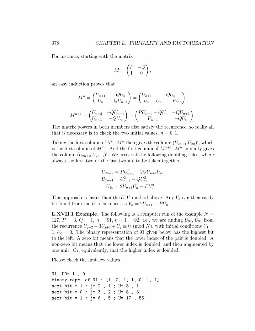
378 CHAPTER L. PRIMALITY AND FACTORIZATION
For instance, starting with the matrix
M =
(P −Q1 0
),
an easy induction proves that
Mn =
(Un+1 −QUn
Un −QUn−1
)=
(Un+1 −QUn
Un Un+1 − PUn
),
Mn+1 =
(Un+2 −QUn+1
Un+1 −QUn
)=
(PUn+1 −QUn −QUn+1
Un+1 −QUn
).
The matrix powers in both members also satisfy the recurrence, so really allthat is necessary is to check the two initial values, n = 0, 1.
Taking the first column of Mn ·Mn then gives the column (U2n+1 U2n)t, whichis the first column of M2n. And the first column of Mn+1 ·Mn similarly givesthe column (U2n+2 U2n+1)
t. We arrive at the following doubling rules, wherealways the first two or the last two are to be taken together:
U2n+2 = PU2n+1 − 2QUn+1Un,
U2n+1 = U2n+1 −QU2
n,
U2n = 2Un+1Un − PU2n.
This approach is faster than the U, V method above. Any Vn can then easilybe found from the U -recurrence, as Vn = 2Un+1 − PUn.
L.XVII.1 Example. The following is a computer run of the example N =127, P = 3, Q = 1, n = 91, n + 1 = 92, i.e., we are finding U92, U91 fromthe recurrence Uj+2− 3Uj+2 +Uj ≡ 0 (mod N), with initial conditions U1 =1, U0 = 0. The binary representation of 91 given below has the highest bitto the left. A zero bit means that the lower index of the pair is doubled. Anon-zero bit means that the lower index is doubled, and then augmented byone unit. Or, equivalently, that the higher index is doubled.
Please check the first few values.
U1, U0= 1 , 0
binary repr. of 91 : [1, 0, 1, 1, 0, 1, 1]
next bit = 1 : j= 2 , 1 ; U= 3 , 1
next bit = 0 : j= 3 , 2 ; U= 8 , 3
next bit = 1 : j= 6 , 5 ; U= 17 , 55

L.XVII. SCALAR FORMULAS 379
next bit = 1 : j= 12 , 11 ; U= 13 , 58
next bit = 0 : j= 23 , 22 ; U= 107 , 52
next bit = 1 : j= 46 , 45 ; U= 105 , 109
next bit = 1 : j= 92 , 91 ; U= 25 , 33
�
An alternative route to these, and many other, identities is to note thata− b =
√D, Un
√D = an − bn, so that:
2an = (an + bn) + (an − bn) = Vn + Un
√D,
an =1
2(Vn + Un
√D).
For instance:
an+1 =1
2(Vn+1 + Un+1
√D) = an · a =
Vn + Un
√D
2· V1 + U1
√D
2.
As the Un and Vn are rational integers, we may identify the rational andirrational parts, and we find again
Un+1 =1
2(VnU1 + UnV1) =
1
2(Vn + PUn),
Vn+1 =1
2(VnV1 + UnU1) =
1
2(PVn + Un).
Details and more identities can also be found in the books of Riesel andBressoud-Wagon. Crandall-Pomerance also give an account, but they usemore Algebra.
L.XVII: Exercises
1. Check the derivation of the update formulas for the (Un+1, Un)-pairs abovefrom the matrix products.
2. Derive as many identities as you possibly can from the relation
an =12(Vn + Un
√D).

380 CHAPTER L. PRIMALITY AND FACTORIZATION
3. (a) Denote the V -sequence belonging to the parameters P, Q by Vn(P,Q).Prove the identity:
Vn(Vk(P, 1), 1) = Vnk(P, 1)
(b) Can you generalize to the case where the first and third 1 are replacedby Q?
(c) Assuming that ((P 2 − 4)/N) = −1, so that ((P 2 − 4)/p) = −1 for atleast one prime factor p of N , that k is a product of prime powers,and n a prime, do you see how the ideas of Pollard’s p − 1 factoringalgorithm (L.VIII) translate to this situation?
(d) A more direct approach to the factoring problem would be to raise oneroot a of the equation X2 − PX + 1 = 0 to high powers modulo N ,again assuming ((P 2 − 4)/N) = −1, Discuss the connection. You mayderive inspiration from the ideas of Berlekamp’s algorithm, E.IV.
4. Suggestions for computing Write a program that computes Uq (mod p)for given parameters P,Q.
Show that n = 323 = 17 ·19 is a Lucas pseudoprime for the parameters P =1, Q = −1, i.e., n is composite, and UN ≡ 0 (mod n) for N = n + (D/n).
5. Let q be a prime number. Determine Vq−(D/n), where D is the discriminantP 2 − 4Q. How does this apply to the previous problem?
Compare these results to the case N = 5777 = 53 · 109.
6. Suppose that (D/n) = −1, but also (Q/n) = +1. Further suppose thatUn+1 ≡ 0 (mod n), and Vn+1 ≡ 2Q (mod n). Let m = (n + 1)/2. Showthat the irrational part of am (the term involving
√D) is congruent to zero
modulo n if and only if Um ≡ 0.
How can this observation be included in a Lucas primality test?
You may want to express both the assumptions and the conclusion in termsof the power sequence an. Cf. the paper by Jon Grantham, “A ProbablePrime Test with High Confidence”, Journal of Number Theory, 72, 32-47(1998), http://www.rni.net/∼pseudoprime/jgpapers.html
7. Under the assumptions of the previous problem, show that U2m+1 ≡ Q
(mod n), even if n is composite.

Bibliography
Elementary
Of the books below Rosen is the most comprehensive, the most consistentlyelementary, and the richest in applications.
Nagell’s book (translated from Swedish) is a very well-organized and well-written account of the elements from a time when the largest known primenumber was 2127 − 1.
Mollin gives the fundaments, but advances to the beginnings of AlgebraicNumber Theory. The book is slanted towards his interests in Pell-type Dio-phantine equations.
Stillwell’s book gives a very gentle introduction to some concepts in AlgebraicNumber Theory.
Childs, L., A Concrete Introduction to Higher Algebra, Springer-Verlag,UTM, 2nd ed., 1995.
Jones, G.A., Jones, J. M., Elementary Number Theory, Springer SUMS,1998.
Mollin, R. A., Fundamental Number Theory with Applications, CRC Press,1998.
Nagell, T., Introduction to Number Theory, Almqvist & Wicksell, Wiley,1951.
Niven, I., Zuckerman, H., Montgomery H., An Introduction to theTheory of Numbers, Wiley.
Rosen, K. H., Elementary Number Theory and its applications, PearsonInternational, 5th ed, 2005.
381

382 BIBLIOGRAPHY
Schumer, P., Introduction to Number Theory, PWS Publishing Co.
Stillwell, J., Elements of Number Theory, Springer-Verlag UTM, 2003.
Computational
The book by Bressoud alone is out of print. It has a good introduction toelliptic curves, and gives most of the background material as it goes along.
The more comprehensive books by Riesel and Crandall-Pomerance comple-ment one another. Riesel’s book gives most of the theoretical backgroundin numerous appendices, and lots of Pascal code. Crandall-Pomerance natu-rally covers more of recent developments. They give the algorithms in C-likepseudocode.
Bach-Shallit gives careful foundations of complexity theory, the theory offinite fields, and a survey of methods assuming the as yet unproved ”Gener-alized Riemann Hypthesis”
Bressoud-Wagon is not purely computational, has lots of entertaining andoriginal material.
Cohen’s book contains lots of elementary material despite its title.
Bach, E., Shallit, J., Algorithmic Number Theory, Vol. 1, MIT Press,1996.
Bressoud, D. M., Factorization and Primality Testing, Springer, 1988.
Bressoud, D.,Wagon, S., A Course in Computational Number Theory,Key College Publishing/Springer, 2000.
Cohen, H., A Course in Computational Algebraic Number Theory, SpringerGraduate Texts in Mathematics, 138, 1995.
Crandall, R., Pomerance, C., Prime Numbers - A Computational Per-spective Springer, 2005.
Riesel, H., Prime Numbers and Computer Methods for Factorization,Birkhauser Progress in Mathematics, vol. 126, 1994.

383
Applied
Books on Cryptography usually include most of the background materialfrom Number Theory. The two books listed below include discussions onseveral Discrete Logarithm algorithms, for instance. Trappe-Washington isthe more comprehensive book, also includes some Coding Theory.
The third book covers an astonishing range of applications, but does notexactly prove everything.
Buchmann, J., Introduction to Cryptography, Springer UTM 2003.
Trappe, W., Washington, L., Introduction to Cryptography with CodingTheory, Prentice Hall, 2002.
Schroeder, M.R., Number Theory in Science and Communication, Springer,1986.
Advanced
The two books listed deal with various advanced topics still mostly outsidethe realm of Algebraic Number Theory. There is very little overlap betweenthe two. Ireland-Rosen presupposes some Abstract Algebra, Rose demandsmore in the way of Analysis.
Ireland, K., Rosen, M., A Classical Introduction to Modern Number The-ory, Springer Graduate Texts 82, 1982.
Rose, H. E., A Course in Number Theory, Oxford Science Publications,1994.
Historic
Scharlau, W., Opolka, H., From Fermat to Minkowski, Lectures on theTheory of Numbers and its Historic Development, Springer UndergraduateTexts, 1984.
Edwards, H. M., Fermat’s Last Theorem, A Genetic Introduction to Alge-braic Number Theory, Springer Graduate Texts in Mathematics 50, 1977.

384 BIBLIOGRAPHY
Analytic
The first title below is an extremely well-written introduction, with full cov-erage of the elementary parts. The second title goes more deeply into theanalytic parts.
Apostol, T., Introduction to Analytic Number Theory, Springer Undergrad-uate Texts, 1976.
Brudern, J., Einfuhrung in die analytische Zahlentheorie, Springer-Lehrbuch,1995.
Elliptic
The books on elliptic curves that seem to require the least preparation are
Silverman, J., Tate, J., Rational Points on Elliptic Curves, SpringerUndergraduate Texts, 1992.
Washington, L., Elliptic Curves, Number Theory and Cryptography, Chap-man & Hall, 2003.
Algebraic
The textbooks below inevitably require some “Abstract” Algebra, but areamong the most concrete and clearly written accounts of the foundations.The essay by R Dedekind has a long and very interesting introduction by J.Stillwell.
Dedekind, R., Theory of Algebraic Integers, Cambridge University Press,in the series “Cambridge Mathematical Library”, 1996 , translated and in-troduced by J. Stillwell.
Holzer, L., Zahlentheorie, Teubner, 1958.
Stewart, I.N., Tall, D.O., Algebraic Number Theory, Chapman and Hall,1979.

385
Articles cited in the text
R. Brent, J. Pollard. “Factorization of the Eighth Fermat Number”. Math-ematics of Computation, Vol. 36, No. 154 (Apr., 1981), pp. 627-630.
J. Brillhart, M. Morrison. “A Method of Factoring and the Factorization ofF7”. Mathematics of Computation, Vol. 29, No. 129 (Jan. 1975), 183-205,
I. Damgard, P. Landrock, C. Pomerance. “Average Case Error for the StrongProbable Prime Test”. Mathematics of Computation, Vol.61 (1993), No.203, pp. 177-194.
M. Gerstenhaber. “The 152nd proof of the law of quadratic reciprocity”.Am. Math. Monthly, 70 (1963), 397-398.
J. Grantham. “A Probable Prime Test with High Confidence”, Journal ofNumber Theory, 72, (1998), 32-47.
Or: http://www.rni.net/∼pseudoprime/jgpapers.html
K. Matthews. “The Diophantine Equation x2 − Dy2 = N,D > 0”, Exposi-tiones Mathematicae, 18 (2000), 323-331.
For complements and corrections, refer to http://www.numbertheory.org/
papers.html#patz
K.Matthews, “The Diophantine equation ax2+bxy+cy2 = N,D = b2−4ac >0”, Journal de Thorie des Nombres de Bordeaux, 14 (2002) 257-270.
Available at the url above.
K. Matthews, “Thue’s theorem and the diophantine equation x2 − Dy2 =±N”, Mathematics of Computation, 71 No. 239 (2001), 1281-1286.
A. Nitaj. “L’algorithme de Cornacchia”, Expositiones Mathematicae 13,(1995), 358-365.
R. Silverman: “The Multiple Polynomial Quadratic Sieve”, Mathematics ofComputation, 48, No 177 (1987), 329-339.

386 BIBLIOGRAPHY
Web
Dario Alpern’s Site. Factoring and Discrete Logarithms with open sourcecode in Java. For Spanish version, delete “ENGLISH.HTM”.
http://www.alpertron.com.ar/ENGLISH.HTM
D. J. Bernstein’s Notes. A set of notes on integer factorization. Bern-stein’s website has lots of interesting material, not all of it related to math-ematics or computer science.
http://cr.yp.to/2006-aws/notes-20060309.pdf
J. Brillhart et al., Factorizations of bn± 1, b = 2, 3, 5, 6, 7, 10, 11, 12, Upto High Powers. Apart from the tables (nice for checking your own results)this book has a very concise resume of the theory and techniques involved,and some fascinating historical comments on the hardware.
http://www.ams.org/online bks/conm22/
S. Contini. Has Contini’s MSc thesis on the ”self-initializing” QuadraticSieve, downloadable in pdf:
http://www.crypto-world.com/Contini.html
W. Hart. Source code for SIMPQS. http://www.friedspace.com/QS/
Ikenaga’s Notes. Conceived as companion notes to Rosen’s text. Thesolution to x2 − 1141y2 = 1 was still wrong in December 2006.
http://marauder.millersville.edu/∼bikenaga/numth/numnote.html
Lenstra, H.W., Jr., Solving the Pell Equation.
http://www.ams.org/notices/200202/fea-lenstra.pdf
The MacTutor History of Mathematics Archive.
http://www-history.mcs.st-andrews.ac.uk/history/Indexes/Number Theory.
html
The Mathematical Atlas.
http://www.math.niu.edu/∼rusin/known-math/index/11-XX.html
Montgomery Survey. A very good survey of modern factorization meth-ods. Downloadable in postscript.

387
http://citeseer.ist.psu.edu/montgomery94survey.html
Number Theory Web.
http://www.numbertheory.org/ntw/
J. Papadoupolos. Source code for msieve, http://www.boo.net/∼jasonp/qs.html
PARI. Computer algebra system designed for fast computations in numbertheory.
http://pari.math.u-bordeaux.fr/
The Prime Pages.
http://primes.utm.edu/
Python Programming Language.
http://www.python.org/
Wikipedia. Often a surprisingly accurate first source (e.g., follow the ex-ternal links).
http://www.wikipedia.org
Wolfram MathWorld.
http://mathworld.wolfram.com/

388 BIBLIOGRAPHY

389

390 TABLES
Tables
x2 −Dy2 = ±1
Lists D : (x, y,±1, period)
2 : (1, 1,−1, 1) 3 : (2, 1, 1, 2) 5 : (2, 1,−1, 1)6 : (5, 2, 1, 2) 7 : (8, 3, 1, 4) 8 : (3, 1, 1, 2)10 : (3, 1,−1, 1) 11 : (10, 3, 1, 2) 12 : (7, 2, 1, 2)13 : (18, 5,−1, 5) 14 : (15, 4, 1, 4) 15 : (4, 1, 1, 2)17 : (4, 1,−1, 1) 18 : (17, 4, 1, 2) 19 : (170, 39, 1, 6)20 : (9, 2, 1, 2) 21 : (55, 12, 1, 6) 22 : (197, 42, 1, 6)23 : (24, 5, 1, 4) 24 : (5, 1, 1, 2) 26 : (5, 1,−1, 1)27 : (26, 5, 1, 2) 28 : (127, 24, 1, 4) 29 : (70, 13,−1, 5)30 : (11, 2, 1, 2) 31 : (1520, 273, 1, 8) 32 : (17, 3, 1, 4)33 : (23, 4, 1, 4) 34 : (35, 6, 1, 4) 35 : (6, 1, 1, 2)37 : (6, 1,−1, 1) 38 : (37, 6, 1, 2) 39 : (25, 4, 1, 2)40 : (19, 3, 1, 2) 41 : (32, 5,−1, 3) 42 : (13, 2, 1, 2)43 : (3482, 531, 1, 10) 44 : (199, 30, 1, 8) 45 : (161, 24, 1, 6)46 : (24335, 3588, 1, 12) 47 : (48, 7, 1, 4) 48 : (7, 1, 1, 2)50 : (7, 1,−1, 1) 51 : (50, 7, 1, 2) 52 : (649, 90, 1, 6)53 : (182, 25,−1, 5) 54 : (485, 66, 1, 6) 55 : (89, 12, 1, 4)56 : (15, 2, 1, 2) 57 : (151, 20, 1, 6 58 : (99, 13,−1, 7)59 : (530, 69, 1, 6) 60 : (31, 4, 1, 4) 61 : (29718, 3805,−1, 11)62 : (63, 8, 1, 4) 63 : (8, 1, 1, 2) 65 : (8, 1,−1, 1)66 : (65, 8, 1, 2) 67 : (48842, 5967, 1, 10) 68 : (33, 4, 1, 2)69 : (7775, 936, 1, 8) 70 : (251, 30, 1, 6) 71 : (3480, 413, 1, 8)72 : (17, 2, 1, 2) 73 : (1068, 125,−1, 7) 74 : (43, 5,−1, 5)75 : (26, 3, 1, 4) 76 : (57799, 6630, 1, 12) 77 : (351, 40, 1, 6)78 : (53, 6, 1, 4) 79 : (80, 9, 1, 4) 80 : (9, 1, 1, 2)82 : (9, 1,−1, 1) 83 : (82, 9, 1, 2) 84 : (55, 6, 1, 2)85 : (378, 41,−1, 5) 86 : (10405, 1122, 1, 10) 87 : (28, 3, 1, 2)88 : (197, 21, 1, 6) 89 : (500, 53,−1, 5) 90 : (19, 2, 1, 2)91 : (1574, 165, 1, 8) 92 : (1151, 120, 1, 8) 93 : (12151, 1260, 1, 10)94 : (2143295, 221064, 1, 16) 95 : (39, 4, 1, 4) 96 : (49, 5, 1, 4)97 : (5604, 569,−1, 11) 98 : (99, 10, 1, 4) 99 : (10, 1, 1, 2)

391
101 : (10, 1,−1, 1) 102 : (101, 10, 1, 2) 103 : (227528, 22419, 1, 12)104 : (51, 5, 1, 2) 105 : (41, 4, 1, 2) 106 : (4005, 389,−1, 9)107 : (962, 93, 1, 6) 108 : (1351, 130, 1, 8) 109 : (8890182, 851525,−1, 15)

392 TABLES
A Table Of Primitive Roots
For every odd prime≤ 5009 the least positive primitive root is listed. Format:[prime, leastprimitiveroot]. 1-1019
[3, 2], [5, 2], [7, 3], [11, 2], [13, 2],[17, 3], [19, 2], [23, 5], [29, 2], [31, 3],[37, 2], [41, 6], [43, 3], [47, 5], [53, 2],[59, 2], [61, 2], [67, 2], [71, 7], [73, 5],[79, 3], [83, 2], [89, 3], [97, 5], [101, 2],[103, 5], [107, 2], [109, 6], [113, 3], [127, 3],[131, 2], [137, 3], [139, 2], [149, 2], [151, 6],[157, 5], [163, 2], [167, 5], [173, 2], [179, 2],[181, 2], [191, 19], [193, 5], [197, 2], [199, 3],[211, 2], [223, 3], [227, 2], [229, 6], [233, 3],[239, 7], [241, 7], [251, 6], [257, 3], [263, 5],[269, 2], [271, 6], [277, 5], [281, 3], [283, 3],[293, 2], [307, 5], [311, 17], [313, 10], [317, 2],[331, 3], [337, 10], [347, 2], [349, 2], [353, 3],[359, 7], [367, 6], [373, 2], [379, 2], [383, 5],[389, 2], [397, 5], [401, 3], [409, 21], [419, 2],[421, 2], [431, 7], [433, 5], [439, 15], [443, 2],[449, 3], [457, 13], [461, 2], [463, 3], [467, 2],[479, 13], [487, 3], [491, 2], [499, 7], [503, 5],[509, 2], [521, 3], [523, 2], [541, 2], [547, 2],[557, 2], [563, 2], [569, 3], [571, 3], [577, 5],[587, 2], [593, 3], [599, 7], [601, 7], [607, 3],[613, 2], [617, 3], [619, 2], [631, 3], [641, 3],[643, 11], [647, 5], [653, 2], [659, 2], [661, 2],[673, 5], [677, 2], [683, 5], [691, 3], [701, 2],[709, 2], [719, 11], [727, 5], [733, 6], [739, 3],[743, 5], [751, 3], [757, 2], [761, 6], [769, 11],[773, 2], [787, 2], [797, 2], [809, 3], [811, 3],[821, 2], [823, 3], [827, 2], [829, 2], [839, 11],[853, 2], [857, 3], [859, 2], [863, 5], [877, 2],[881, 3], [883, 2], [887, 5], [907, 2], [911, 17],[919, 7], [929, 3], [937, 5], [941, 2], [947, 2],[953, 3], [967, 5], [971, 6], [977, 3], [983, 5],[991, 6], [997, 7], [1009, 11], [1013, 3], [1019, 2]

393
1021-2579
[1021, 10], [1031, 14], [1033, 5], [1039, 3], [1049, 3],[1051, 7], [1061, 2], [1063, 3], [1069, 6], [1087, 3],[1091, 2], [1093, 5], [1097, 3], [1103, 5], [1109, 2],[1117, 2], [1123, 2], [1129, 11], [1151, 17], [1153, 5],[1163, 5], [1171, 2], [1181, 7], [1187, 2], [1193, 3],[1201, 11], [1213, 2], [1217, 3], [1223, 5], 1229, 2],[1231, 3], [1237, 2], [1249, 7], [1259, 2], [1277, 2],[1279, 3], [1283, 2], [1289, 6], [1291, 2], [1297, 10],[1301, 2], 1303, 6], [1307, 2], [1319, 13], [1321, 13],[1327, 3], [1361, 3], [1367, 5], [1373, 2], [1381, 2],[1399, 13], [1409, 3], [1423, 3], [1427, 2], [1429, 6],[1433, 3], [1439, 7], [1447, 3], [1451, 2], [1453, 2],[1459, 3], [1471, 6], [1481, 3], [1483, 2], [1487, 5],[1489, 14], [1493, 2], [1499, 2], [1511, 11], [1523, 2],[1531, 2], [1543, 5], [1549, 2], [1553, 3], [1559, 19],[1567, 3], [1571, 2], [1579, 3], [1583, 5], [1597, 11],[1601, 3], [1607, 5], [1609, 7], [1613, 3], [1619, 2],[1621, 2], [1627, 3], [1637, 2], [1657, 11], [1663, 3],[1667, 2], [1669, 2], [1693, 2], [1697, 3], [1699, 3],[1709, 3], [1721, 3], [1723, 3], [1733, 2], [1741, 2],[1747, 2], [1753, 7], [1759, 6], [1777, 5], [1783, 10],[1787, 2], [1789, 6], [1801, 11], [1811, 6], [1823, 5],[1831, 3], [1847, 5], [1861, 2], [1867, 2], [1871, 14],[1873, 10], [1877, 2], [1879, 6], [1889, 3], [1901, 2],[1907, 2], [1913, 3], [1931, 2], [1933, 5], [1949, 2],[1951, 3], [1973, 2], [1979, 2], [1987, 2], [1993, 5][1997, 2], [1999, 3], [2003, 5], [2011, 3], [2017, 5],[2027, 2], [2029, 2], [2039, 7], [2053, 2], [2063, 5],[2069, 2], [2081, 3], [2083, 2], [2087, 5], [2089, 7],[2099, 2], [2111, 7], [2113, 5], [2129, 3], [2131, 2],[2137, 10], [2141, 2], [2143, 3], [2153, 3], [2161, 23],[2179, 7], [2203, 5], [2207, 5], [2213, 2], [2221, 2],[2237, 2], [2239, 3], [2243, 2], [2251, 7], [2267, 2],[2269, 2], [2273, 3], [2281, 7], [2287, 19], [2293, 2],[2297, 5], [2309, 2], [2311, 3], [2333, 2], [2339, 2],[2341, 7], [2347, 3], [2351, 13], [2357, 2], [2371, 2],[2377, 5], [2381, 3], [2383, 5], [2389, 2], [2393, 3],[2399, 11], [2411, 6], [2417, 3], [2423, 5], [2437, 2],[2441, 6], [2447, 5], 2459, 2], [2467, 2], [2473, 5],[2477, 2], [2503, 3], [2521, 17], [2531, 2], [2539, 2],[2543, 5], [2549, 2], [2551, 6], [2557, 2], [2579, 2],

394 TABLES
2591-4001
[2591, 7], [2593, 7], [2609, 3], [2617, 5], [2621, 2],[2633, 3], [2647, 3], [2657, 3], [2659, 2], [2663, 5],[2671, 7], [2677, 2], [2683, 2], [2687, 5], [2689, 19],[2693, 2], [2699, 2], [2707, 2], [2711, 7], [2713, 5],[2719, 3], [2729, 3], [2731, 3], [2741, 2], [2749, 6],[2753, 3], [2767, 3], [2777, 3], [2789, 2], [2791, 6],[2797, 2], [2801, 3], [2803, 2], [2819, 2], [2833, 5],[2837, 2], [2843, 2], [2851, 2], [2857, 11], [2861, 2],[2879, 7], [2887, 5], 2897, 3], [2903, 5], [2909, 2],[2917, 5], [2927, 5], [2939, 2], [2953, 13], [2957, 2],[2963, 2], [2969, 3], [2971, 10], [2999, 17], [3001, 14][3011, 2], [3019, 2], [3023, 5], [3037, 2], [3041, 3],[3049, 11], [3061, 6], [3067, 2], [3079, 6], [3083, 2],[3089, 3], [3109, 6], [3119, 7], [3121, 7], [3137, 3],[3163, 3], [3167, 5], [3169, 7], [3181, 7], [3187, 2],[3191, 11], [3203, 2], [3209, 3], [3217, 5], [3221, 10],[3229, 6], [3251, 6], [3253, 2], [3257, 3], [3259, 3],[3271, 3], [3299, 2], [3301, 6], [3307, 2], [3313, 10],[3319, 6], [3323, 2], [3329, 3], [3331, 3], [3343, 5],[3347, 2], [3359, 11], [3361, 22], [3371, 2], [3373, 5],[3389, 3], [3391, 3], [3407, 5], [3413, 2], [3433, 5],[3449, 3], [3457, 7], [3461, 2], [3463, 3], [3467, 2],[3469, 2], [3491, 2], [3499, 2], [3511, 7], [3517, 2],[3527, 5], [3529, 17], [3533, 2], [3539, 2], [3541, 7],[3547, 2], [3557, 2], [3559, 3], [3571, 2], [3581, 2],[3583, 3], [3593, 3], [3607, 5], [3613, 2], [3617, 3],[3623, 5], [3631, 15], [3637, 2], [3643, 2], [3659, 2],[3671, 13], 3673, 5], [3677, 2], [3691, 2], [3697, 5],[3701, 2], [3709, 2], [3719, 7], [3727, 3], [3733, 2],[3739, 7], [3761, 3], [3767, 5], [3769, 7], [3779, 2],[3793, 5], [3797, 2], [3803, 2], [3821, 3], [3823, 3],[3833, 3], [3847, 5], [3851, 2], [3853, 2], [3863, 5],[3877, 2], [3881, 13], [3889, 11], [3907, 2], [3911, 13],[3917, 2], [3919, 3], [3923, 2], [3929, 3], [3931, 2],[3943, 3], [3947, 2], [3967, 6], [3989, 2], [4001, 3],

395
4003-5009
[4003, 2], [4007, 5], [4013, 2], [4019, 2], [4021, 2],[4027, 3], [4049, 3], [4051, 10], [4057, 5], [4073, 3],[4079, 11], [4091, 2], [4093, 2], [4099, 2], [4111, 12],[4127, 5], [4129, 13], [4133, 2], [4139, 2], [4153, 5],[4157, 2], [4159, 3], [4177, 5], [4201, 11], [4211, 6],[4217, 3], [4219, 2], [4229, 2], [4231, 3], [4241, 3],[4243, 2], [4253, 2], [4259, 2], [4261, 2], [4271, 7],[4273, 5], [4283, 2], [4289, 3], [4297, 5], [4327, 3],[4337, 3], [4339, 10], [4349, 2], [4357, 2], [4363, 2],[4373, 2], [4391, 14], [4397, 2], [4409, 3], [4421, 3],[4423, 3], [4441, 21], [4447, 3], [4451, 2], [4457, 3],[4463, 5], [4481, 3], [4483, 2], [4493, 2], [4507, 2],[4513, 7], [4517, 2], [4519, 3], [4523, 5], [4547, 2],[4549, 6], [4561, 11], [4567, 3], [4583, 5], [4591, 11],[4597, 5], [4603, 2], [4621, 2], [4637, 2], [4639, 3],[4643, 5], [4649, 3], [4651, 3], [4657, 15], [4663, 3],[4673, 3], [4679, 11], [4691, 2], [4703, 5], [4721, 6],[4723, 2], [4729, 17], [4733, 5], [4751, 19], [4759, 3],[4783, 6], [4787, 2], [4789, 2], [4793, 3], [4799, 7],[4801, 7], [4813, 2], [4817, 3], [4831, 3], [4861, 11],[4871, 11], [4877, 2], [4889, 3], [4903, 3], [4909, 6],[4919, 13], [4931, 6], [4933, 2], [4937, 3], [4943, 7],[4951, 6], [4957, 2], [4967, 5], [4969, 11], [4973, 2],[4987, 2], [4993, 5], [4999, 3], [5003, 2], [5009, 3].
A Table of Discrete Logarithms
Primitive root =2, unless otherwise noted.
prime=3
[1, 2], [2, 1]
prime=5
[1, 4], [2, 1], [3, 3], [4, 2]
prime=7, primitive root = 3
[1, 6], [2, 2], [3, 1], [4, 4], [5, 5], [6, 3]

396 TABLES
prime=11, primitive root =2
[1, 10], [2, 1], [3, 8], [4, 2], [5, 4], [6, 9], [7, 7], [8, 3],
[9,6], [10, 5]
prime=13
[1, 12], [2, 1], [3, 4], [4, 2], [5, 9], [6, 5], [7, 11], [8, 3], [9,
8], [10, 10], [11, 7], [12, 6]
prime=17, primitive root =3
[1, 16], [2, 14], [3, 1], [4, 12], [5, 5], [6, 15], [7, 11], [8, 10],
[9, 2], [10, 3], [11, 7], [12, 13], [13, 4], [14, 9], [15, 6], [16,
8]
prime=19
[1, 18], [2, 1], [3, 13], [4, 2], [5, 16], [6, 14], [7, 6], [8, 3],
[9, 8], [10, 17], [11, 12], [12, 15], [13, 5], [14, 7], [15, 11],
[16,4], [17, 10], [18, 9]
prime=23, primitive root = 5
[1, 22], [2, 2], [3, 16], [4, 4], [5, 1], [6, 18], [7, 19], [8, 6],
[9, 10], [10, 3], [11, 9], [12, 20], [13, 14], [14, 21], [15, 17],
[16, 8], [17, 7], [18, 12], [19, 15], [20, 5], [21, 13], [22, 11]
prime=29
[1, 28], [2, 1], [3, 5], [4, 2], [5, 22], [6, 6], [7, 12], [8, 3],
[9, 10], [10, 23], [11, 25], [12, 7], [13, 18], [14, 13], [15, 27],
[16, 4], [17, 21], [18, 11], [19, 9], [20, 24], [21, 17], [22, 26],
[23, 20], [24, 8], [25, 16], [26, 19], [27, 15], [28, 14]
prime=31, primitive root =3
[1, 30], [2, 24], [3, 1], [4, 18], [5, 20], [6, 25], [7, 28],
[8,12], [9, 2], [10, 14], [11, 23], [12, 19], [13, 11], [14, 22],
[15,21], [16, 6], [17, 7], [18, 26], [19, 4], [20, 8], [21, 29], [22, 17],
[23, 27], [24, 13], [25, 10], [26, 5], [27, 3], [28, 16], [29, 9],
[30, 15]
prime=37
[1, 36], [2, 1], [3, 26], [4, 2], [5, 23], [6, 27], [7, 32], [8, 3],
[9, 16], [10, 24], [11, 30], [12, 28], [13, 11], [14, 33], [15, 13],
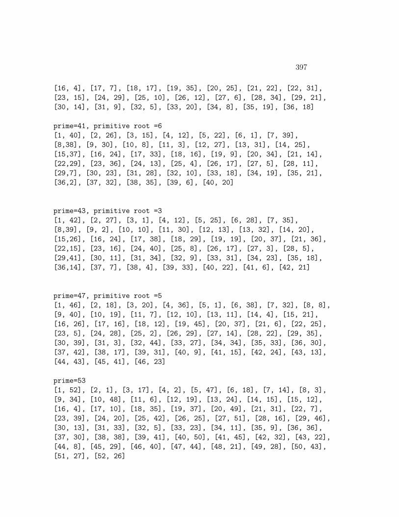
397
[16, 4], [17, 7], [18, 17], [19, 35], [20, 25], [21, 22], [22, 31],
[23, 15], [24, 29], [25, 10], [26, 12], [27, 6], [28, 34], [29, 21],
[30, 14], [31, 9], [32, 5], [33, 20], [34, 8], [35, 19], [36, 18]
prime=41, primitive root =6
[1, 40], [2, 26], [3, 15], [4, 12], [5, 22], [6, 1], [7, 39],
[8,38], [9, 30], [10, 8], [11, 3], [12, 27], [13, 31], [14, 25],
[15,37], [16, 24], [17, 33], [18, 16], [19, 9], [20, 34], [21, 14],
[22,29], [23, 36], [24, 13], [25, 4], [26, 17], [27, 5], [28, 11],
[29,7], [30, 23], [31, 28], [32, 10], [33, 18], [34, 19], [35, 21],
[36,2], [37, 32], [38, 35], [39, 6], [40, 20]
prime=43, primitive root =3
[1, 42], [2, 27], [3, 1], [4, 12], [5, 25], [6, 28], [7, 35],
[8,39], [9, 2], [10, 10], [11, 30], [12, 13], [13, 32], [14, 20],
[15,26], [16, 24], [17, 38], [18, 29], [19, 19], [20, 37], [21, 36],
[22,15], [23, 16], [24, 40], [25, 8], [26, 17], [27, 3], [28, 5],
[29,41], [30, 11], [31, 34], [32, 9], [33, 31], [34, 23], [35, 18],
[36,14], [37, 7], [38, 4], [39, 33], [40, 22], [41, 6], [42, 21]
prime=47, primitive root =5
[1, 46], [2, 18], [3, 20], [4, 36], [5, 1], [6, 38], [7, 32], [8, 8],
[9, 40], [10, 19], [11, 7], [12, 10], [13, 11], [14, 4], [15, 21],
[16, 26], [17, 16], [18, 12], [19, 45], [20, 37], [21, 6], [22, 25],
[23, 5], [24, 28], [25, 2], [26, 29], [27, 14], [28, 22], [29, 35],
[30, 39], [31, 3], [32, 44], [33, 27], [34, 34], [35, 33], [36, 30],
[37, 42], [38, 17], [39, 31], [40, 9], [41, 15], [42, 24], [43, 13],
[44, 43], [45, 41], [46, 23]
prime=53
[1, 52], [2, 1], [3, 17], [4, 2], [5, 47], [6, 18], [7, 14], [8, 3],
[9, 34], [10, 48], [11, 6], [12, 19], [13, 24], [14, 15], [15, 12],
[16, 4], [17, 10], [18, 35], [19, 37], [20, 49], [21, 31], [22, 7],
[23, 39], [24, 20], [25, 42], [26, 25], [27, 51], [28, 16], [29, 46],
[30, 13], [31, 33], [32, 5], [33, 23], [34, 11], [35, 9], [36, 36],
[37, 30], [38, 38], [39, 41], [40, 50], [41, 45], [42, 32], [43, 22],
[44, 8], [45, 29], [46, 40], [47, 44], [48, 21], [49, 28], [50, 43],
[51, 27], [52, 26]

398 TABLES
prime=59
[1, 58], [2, 1], [3, 50], [4, 2], [5, 6], [6, 51], [7, 18], [8, 3],
[9, 42], [10, 7], [11, 25], [12, 52], [13, 45], [14, 19], [15, 56],
[16, 4], [17, 40], [18, 43], [19, 38], [20, 8], [21, 10], [22, 26],
[23, 15], [24, 53], [25, 12], [26, 46], [27, 34], [28, 20], [29, 28],
[30, 57], [31, 49], [32, 5], [33, 17], [34, 41], [35, 24], [36, 44],
[37, 55], [38, 39], [39, 37], [40, 9], [41, 14], [42, 11], [43, 33],
[44, 27], [45, 48], [46, 16], [47, 23], [48, 54], [49, 36], [50, 13],
[51, 32], [52, 47], [53, 22], [54, 35], [55, 31], [56, 21], [57, 30],
[58, 29]
prime=61
[1, 60], [2, 1], [3, 6], [4, 2], [5, 22], [6, 7], [7, 49], [8, 3],
[9, 12], [10, 23], [11, 15], [12, 8], [13, 40], [14, 50], [15, 28],
[16, 4], [17, 47], [18, 13], [19, 26], [20, 24], [21, 55], [22, 16],
[23, 57], [24, 9], [25, 44], [26, 41], [27, 18], [28, 51], [29, 35],
[30, 29], [31, 59], [32, 5], [33, 21], [34, 48], [35, 11], [36, 14],
[37, 39], [38, 27], [39, 46], [40, 25], [41, 54], [42, 56], [43, 43],
[44, 17], [45, 34], [46, 58], [47, 20], [48, 10], [49, 38], [50, 45],
[51, 53], [52, 42], [53, 33], [54, 19], [55, 37], [56, 52], [57, 32],
[58, 36], [59, 31], [60, 30]
prime=67
[1, 66], [2, 1], [3, 39], [4, 2], [5, 15], [6, 40], [7, 23], [8, 3],
[9, 12], [10, 16], [11, 59], [12, 41], [13, 19], [14, 24], [15, 54],
[16, 4], [17, 64], [18, 13], [19, 10], [20, 17], [21, 62], [22, 60],
[23, 28], [24, 42], [25, 30], [26, 20], [27, 51], [28, 25], [29, 44],
[30, 55], [31, 47], [32, 5], [33, 32], [34, 65], [35, 38], [36, 14],
[37, 22], [38, 11], [39, 58], [40, 18], [41, 53], [42, 63], [43, 9],
[44, 61], [45, 27], [46, 29], [47, 50], [48, 43], [49, 46], [50, 31],
[51, 37], [52, 21], [53, 57], [54, 52], [55, 8], [56, 26], [57, 49],
[58, 45], [59, 36], [60, 56], [61, 7], [62, 48], [63, 35], [64, 6],
[65, 34], [66, 33]
prime=71, primitive root =7
[1, 70], [2, 6], [3, 26], [4, 12], [5, 28], [6, 32], [7, 1], [8, 18],
[9, 52], [10, 34], [11, 31], [12, 38], [13, 39], [14, 7], [15, 54],
[16, 24], [17, 49], [18, 58], [19, 16], [20, 40], [21, 27], [22, 37],
[23, 15], [24, 44], [25, 56], [26, 45], [27, 8], [28, 13], [29, 68],
[30, 60], [31, 11], [32, 30], [33, 57], [34, 55], [35, 29], [36, 64],

399
[37, 20], [38, 22], [39, 65], [40, 46], [41, 25], [42, 33], [43, 48],
[44, 43], [45, 10], [46, 21], [47, 9], [48, 50], [49, 2], [50, 62],
[51, 5], [52, 51], [53, 23], [54, 14], [55, 59], [56, 19], [57, 42],
[58, 4], [59, 3], [60, 66], [61, 69], [62, 17], [63, 53], [64, 36],
[65, 67], [66, 63], [67, 47], [68, 61], [69, 41], [70, 35]
prime=73, primitive root = 5
[1, 72], [2, 8], [3, 6], [4, 16], [5, 1], [6, 14], [7, 33], [8, 24],
[9, 12], [10, 9], [11, 55], [12, 22], [13, 59], [14, 41], [15, 7],
[16, 32], [17, 21], [18, 20], [19, 62], [20, 17], [21, 39], [22, 63],
[23, 46], [24, 30], [25, 2], [26, 67], [27, 18], [28, 49], [29, 35],
[30, 15], [31, 11], [32, 40], [33, 61], [34, 29], [35, 34], [36, 28],
[37, 64], [38, 70], [39, 65], [40, 25], [41, 4], [42, 47], [43, 51],
[44, 71], [45, 13], [46, 54], [47, 31], [48, 38], [49, 66], [50, 10],
[51, 27], [52, 3], [53, 53], [54, 26], [55, 56], [56, 57], [57, 68],
[58, 43], [59, 5], [60, 23], [61, 58], [62, 19], [63, 45], [64, 48],
[65, 60], [66, 69], [67, 50], [68, 37], [69, 52], [70, 42], [71, 44],
[72, 36]
prime=79, primitive root =3
[1, 78], [2, 4], [3, 1], [4, 8], [5, 62], [6, 5], [7, 53], [8, 12],
[9, 2], [10, 66], [11, 68], [12, 9], [13, 34], [14, 57], [15, 63],
[16, 16], [17, 21], [18, 6], [19, 32], [20, 70], [21, 54], [22, 72],
[23, 26], [24, 13], [25, 46], [26, 38], [27, 3], [28, 61], [29, 11],
[30, 67], [31, 56], [32, 20], [33, 69], [34, 25], [35, 37], [36, 10],
[37, 19], [38, 36], [39, 35], [40, 74], [41, 75], [42, 58], [43, 49],
[44, 76], [45, 64], [46, 30], [47, 59], [48, 17], [49, 28], [50, 50],
[51, 22], [52, 42], [53, 77], [54, 7], [55, 52], [56, 65], [57, 33],
[58, 15], [59, 31], [60, 71], [61, 45], [62, 60], [63, 55], [64, 24],
[65, 18], [66, 73], [67, 48], [68, 29], [69, 27], [70, 41], [71, 51],
[72, 14], [73, 44], [74, 23], [75, 47], [76, 40], [77, 43], [78, 39]
prime=83
[1, 82], [2, 1], [3, 72], [4, 2], [5, 27], [6, 73], [7, 8], [8, 3],
[9, 62], [10, 28], [11, 24], [12, 74], [13, 77], [14, 9], [15, 17],
[16, 4], [17, 56], [18, 63], [19, 47], [20, 29], [21, 80], [22, 25],
[23, 60], [24, 75], [25, 54], [26, 78], [27, 52], [28, 10], [29, 12],
[30, 18], [31, 38], [32, 5], [33, 14], [34, 57], [35, 35], [36, 64],
[37, 20], [38, 48], [39, 67], [40, 30], [41, 40], [42, 81], [43, 71],
[44, 26], [45, 7], [46, 61], [47, 23], [48, 76], [49, 16], [50, 55],
[51, 46], [52, 79], [53, 59], [54, 53], [55, 51], [56, 11], [57, 37],

400 TABLES
[58, 13], [59, 34], [60, 19], [61, 66], [62, 39], [63, 70], [64, 6],
[65, 22], [66, 15], [67, 45], [68, 58], [69, 50], [70, 36], [71, 33],
[72, 65], [73, 69], [74, 21], [75, 44], [76, 49], [77, 32], [78, 68],
[79, 43], [80, 31], [81, 42], [82, 41]
prime=89, primitive root = 3
[1, 88], [2, 16], [3, 1], [4, 32], [5, 70], [6, 17], [7, 81],
[8,48], [9, 2], [10, 86], [11, 84], [12, 33], [13, 23], [14, 9],
[15,71], [16, 64], [17, 6], [18, 18], [19, 35], [20, 14], [21, 82],
[22,12], [23, 57], [24, 49], [25, 52], [26, 39], [27, 3], [28, 25],
[29,59], [30, 87], [31, 31], [32, 80], [33, 85], [34, 22], [35, 63],
[36,34], [37, 11], [38, 51], [39, 24], [40, 30], [41, 21], [42, 10],
[43,29], [44, 28], [45, 72], [46, 73], [47, 54], [48, 65], [49, 74],
[50,68], [51, 7], [52, 55], [53, 78], [54, 19], [55, 66], [56, 41],
[57,36], [58, 75], [59, 43], [60, 15], [61, 69], [62, 47], [63, 83],
[64,8], [65, 5], [66, 13], [67, 56], [68, 38], [69, 58], [70, 79],
[71,62], [72, 50], [73, 20], [74, 27], [75, 53], [76, 67], [77, 77],
[78,40], [79, 42], [80, 46], [81, 4], [82, 37], [83, 61], [84, 26],
[85,76], [86, 45], [87, 60], [88, 44]
prime=97, primitive root =5
[1, 96], [2, 34], [3, 70], [4, 68], [5, 1], [6, 8], [7, 31], [8, 6],
[9, 44], [10, 35], [11, 86], [12, 42], [13, 25], [14, 65], [15, 71],
[16, 40], [17, 89], [18, 78], [19, 81], [20, 69], [21, 5], [22, 24],
[23, 77], [24, 76], [25, 2], [26, 59], [27, 18], [28, 3], [29, 13],
[30, 9], [31, 46], [32, 74], [33, 60], [34, 27], [35, 32], [36, 16],
[37, 91], [38, 19], [39, 95], [40, 7], [41, 85], [42, 39], [43, 4],
[44, 58], [45, 45], [46, 15], [47, 84], [48, 14], [49, 62], [50, 36],
[51, 63], [52, 93], [53, 10], [54, 52], [55, 87], [56, 37], [57, 55],
[58, 47], [59, 67], [60, 43], [61, 64], [62, 80], [63, 75], [64, 12],
[65, 26], [66, 94], [67, 57], [68, 61], [69, 51], [70, 66], [71, 11],
[72, 50], [73, 28], [74, 29], [75, 72], [76, 53], [77, 21], [78, 33],
[79, 30], [80, 41], [81, 88], [82, 23], [83, 17], [84, 73], [85, 90],
[86, 38], [87, 83], [88, 92], [89, 54], [90, 79], [91, 56], [92, 49],
[93, 20], [94, 22], [95, 82], [96, 48]

Index
algebraic congruence, 53, 56, 60algebraic integer, 292Alice, 34, 95, 123, 165, 166arithmetic function, 167associate, 295, 297
Bezout identity, 3baby steps, giant steps, 98BBS bit generator, 165belong(ing) to, 217, 240Berlekamp, 161best rational approximation, 206, 230binomial congruence, 76bitwise logic, 6, 112, 166, 322, 356Bob, 34, 95, 123, 165, 166Burnside’s counting theorem, 182
cancellation, 17Carmichael function, 88Carmichael number, 321CFRAC, 347Chinese remainder theorem, 38, 48,
50, 64, 89, 165Chinese remaindering, 96coloring, 181column operation, 199, 200computation of π, 301congruent, 13conjugate, 227, 293continued fraction, 195, 210, 344, 347convergent, 198, 211, 233Cornacchia’s Algorithm, 216cyclotomic polynomial, 187, 188
decimal fraction, 26, 27, 74, 215
Diophantine equation, 143, 154, 156,216, 220, 235, 243, 277, 280,281, 283, 294, 381
Dirichlet inverse, 169, 175, 187Dirichlet product, 169Dirichlet’s theorem, 192discrete logarithm, 94
computation, 95discriminant, 247, 251divisibility theorem
first, 7, 9, 29, 145, 298second, 7, 29, 298
division in number ring, 296, 308
early abort, 348Eisenstein, 129electronic coin flipping, 165ElGamal, 95equivalent quadratic irrationalities, 257,
258Erganzungssatz, 110Euclidean algorithm, 3, 157Euler phi function, 21, 44, 168, 174Euler’s criterion, 76, 108, 121, 332,
366Euler’s theorem, 25, 183Eve, 123extended Euclid, 5, 15, 213
factor base, 100fast exponentiation, 81, 163, 320, 342,
377Fermat number, 314, 331Fermat’s last theorem, 159
401

402 INDEX
field, 291finite, 376
finite continued fraction, 213floor, 196, 226freshman’s dream, 23, 110, 365
Gauß’ lemma, 123, 127Gaussian elimination, 347, 354Gerstenhaber, 129Gray code, 164greatest common divisor, 2, 297
Hensel’s lemma, 62
idempotent, 41inclusion-exclusion principle, 46index, 94index calculus algorithm, 100inverse, 14invertible class, 14irreducible, 293
Jacobi symbol, 118, 333
Lagrange’s product formula, 273, 274Lagrange’s theorem, 56, 72, 376large prime variation, 331, 348least common multiple, 37Legendre symbol, 108linear congruence, 54linear congruential generator, 92linear Diophantine equation, 2, 7, 38little Fermat, 24, 183, 321, 365Lucas sequence, 362
Mobius function, 172, 187Mobius inversion, 172, 182matrix notation, 255Mersenne
number, 185, 314, 330, 371prime, 185, 314, 371
modular square root, 57, 84, 160, 374moving forward one period, 271
multiplicative function, 167multiplicity, 48, 82
Newton method, 345norm, 293, 294, 311
order, 22of a product, 29of a power, 28
partial quotient, 197Pell’s equation, 208, 228Pell-type equation, 277, 283perfect number, 185periodic continued fraction, 212, 231,
247Pohlig-Hellman, 96, 104Pollard p− 1, 335Pollard rho
discrete log, 102factoring, 336
Pratt certificate, 339preperiod of continued fraction, 288primality test
Fermat, 321Lucas-Lehmer, 371Miller, 121Miller-Rabin, 321Pepin, 331Pocklington, 328, 340Proth, 332Solovay-Strassen, 121
primitive root, 69, 179modulo prime, 72modulo prime power, 81
primitive root criterion, 327proper representation, 151, 217, 308pseudoprime, 31pseudorandom, 92, 166, 215purely periodic, 254Pythagorean triples, 11

INDEX 403
QCF, 228, 270, 278, 344quadratic irrationality, 211, 223, 247
reduced, 248, 254, 259quadratic number
field, 293quadratic reciprocity
proof, 127, 129, 280stated, 112
quadratic residue, 107, 347quadratic sieve, 358
reciprocal expansions, 266self-, 268, 275
reciprocal polynomial, 191relatively prime, 3, 37repunit, 315residue class, 12Riesel-Morrison, 367ring, 291root of unity, 187RSA, 33running a period backwards, 275
shift, 6, 322, 356sieve of Eratosthenes, 317strong pseudoprime, 323sum of divisors, 184sum of squares, 143, 270summatory function, 169supplementary theorem
first, 110second, 110, 125
Taylor’s theorem, 61Thue’s lemma, 143, 156, 158tournament, 17trial division, 317
ultimately periodic, 251unique factorization, 10, 291, 299, 309unit, 293, 294
vertical distance, 195
wait for a square, 344Wilson’s theorem, 57, 58, 79
zero-divisor, 14