Elementary Data Structures and Recurrence Equationsfmt.cs.utwente.nl/courses/adc/lec2.pdfRecurrence...

Elementary Data Structures andRecurrence Equations

Lecture #2 of Algorithms, Data structures and Complexity

Joost-Pieter Katoen

Formal Methods and Tools Group

E-mail: [email protected]

September 3, 2002

c� JPK

#2: Data Structures + Recurrence Equations ADC (214020)

Overview� Abstract data types

– Specification versus implementation

� Elementary data structures

– Stacks, (priority) queues and (binary) trees

� Recurrence equations

– Computing Fibonacci numbers

� Solving recurrence equations

– Subtitution method– Recurrence tree method– Master method

c� JPK 1


Abstract data types

� An abstract data type (ADT) consists of: � Java collection

– a data structure, and– a collection of operations

(e.g., constructors, manipulation and access functions)

� Example ADTs: list, tree, stack, queue, priority queue, dictionary � � �

� Clear distinction between:

– how data objects behave and– how they are implemented

� This paradigm is also called data encapsulation (or data abstraction):

– data is only accessible outside the ADT via well-defined operations– the representation of data is only relevant to the implementation

� Distinguish between ADT specification and ADT implementation

c� JPK 2


ADT specification

� An ADT specification: � Java abstract class

– describes how the operations on the data objects behave– neither describes the internal representation of the data objects– nor the implementation of the operations

� They are “off-the-shelf” components to construct our algorithms

� The effect of operations is described by logical relations:

– precondition: statement to be true on calling the operation (user obligation!)– postcondition: statement to be true on result of the operation

� Basis for reasoning about the correctness of the ADT

� Example operation push(Stack � , Object � )

– precondition: true (i.e., vacuous statement)– postcondition: top of stack � = �

c� JPK 3


ADT implementation

� An ADT specification: � Java class

– details how the operations are implemented– details the internal representation of the data objects

� Having different ADT implementations of the same ADT specificationenables us to optimize performance

� Basis for reasoning about the efficiency of the ADT

� Example: push(Stack � , Object � ) for an array-implementation

void push � Stack � � int � � �top � � � � top � � ��

� � top � � � � � �

c� JPK 4


Efficiency of ADT implementations

efficiency of ADT implementations is of vital importance

� The time complexity of the operations on the ADT

– the insertion of data objects– the deletion of data objects– searching for data objects (i.e., look-up)

� The space complexity of the internal data representation

� There is typically a trade-off between time- and data efficiency

– fast data operations typically require extra storage (i.e., bytes)– compact storage often leads to slower operations

� Example: implementation of a priority queue

c� JPK 5










c� JPK 6


Example ADTs: Stacks and queues

� A stack � stores a collection of objects and supports operations:

– isEmpty( � ) returns true if � is empty, and false otherwise– push( � � � ) inserts element � into the stack �

– pop( � ) removes the most recently inserted element and returns it;requires non-empty �

� A queue � stores a collection of objects and supports operations:

– isEmpty( � ) returns true if � is empty, and false otherwise– enqueue( � � � ) inserts element � into the queue �– dequeue( � ) removes the element inserted the longest time ago and returns it;

requires non-empty �

� A stack supports last-in first-out operations, a queue first-in first-out

c� JPK 7


Stack implementation using unbounded arrays (I)

34

3

11

top34

3

11

top41

34

3

11

41

top11

34

3

11

top41

push(11)push(41) pop()

c� JPK 8


Stack implementation using unbounded arrays (II)

bool isEmpty � Stack � � �

return � top � � � � � � � �

void push � Stack � � int � � �

top � � � � top � � ��

� � top � � � � � �

int pop � Stack � � �top � � � � top � � � � � �

return � � top � � �� All operations take � �� time

a linked-list implementation avoids a priori declaration of array size

for pop no test for empty stack necessary; Why?

c� JPK 9


Queue implementation using bounded arrays (I)

1217

tail

head1217

head

tail

0

1217

head

0

9

tail

170

9

tail

head

enq(0) enq(9) deq() deq()

0

9

tail

head

c� JPK 10


Queue implementation using bounded arrays (II)

bool isEmpty � Queue � � �

return � head � � � � � tail � � � � �

void enqueue � Queue � � int � � �

� � tail � � � � � �tail � � � � � tail � � �� mod � �

int dequeue � Queue � � �

int � �� head � � � �

head � � � � � head � � �� mod � �

return � �

All operations take � �� time

for simplicity, overflow is not detected

any alternative implementations?

c� JPK 11


The ADT priority queue

� Consider objects that are equipped with a key (or, priority)

– assume each key is associated to at most one data object

� Objects are ordered according to their priority

� A priority queue � � stores a collection of such objects and supports:

– isEmpty( � � ) returns true if � � is empty, and false otherwise– insert(� � � � �� ) inserts element � with key� into the queue � �

– getMin(� � ) returns the element with smallest key; requires non-empty � �

– delMin(� � ) deletes the element with smallest key; requires non-empty � �

– getElt(� � �� ) returns object � with key� in � � ; requires� to be in � �

– decrKey( � � � � �� ) sets key of � to� ; requires � in � � and� � getKey � � � � � �

� Important data structure for greedy algorithms, discrete-eventsimulation, ...

comparable to the Java Map class (java.util)

c� JPK 12


An unsorted bounded array implementation

tail

head1712

48

head1712

48

tail

0 12

head1712

48

0 12

3 7

tail

head12 80 123 7

tail

ins(0,12) ins(3,7) delMin() getKey(0)

c� JPK 13


A sorted bounded array implementation

ins(0,12) ins(3,7) delMin() getKey(0)

tail

head1712

48 head

tail

0 1212

48

17head

tail

17 47

12

3

0

812

tail0 12

123

87

head

c� JPK 14


Comparing two priority queue implementationsImplementation Unsorted array Sorted array

Operation

isEmpty(� � ) � � � � � � � �

insert(� � � � �� ) � � � � � ��

getMin( � � ) � ��

delMin(� � ) � ��

getElt(� � �� ) � ��

decrKey( � � � � �� ) � ��

� this includes shifting all elements “to the right” of�

� � using binary search

we will consider yet another implementation in lecture # 3!

c� JPK 15


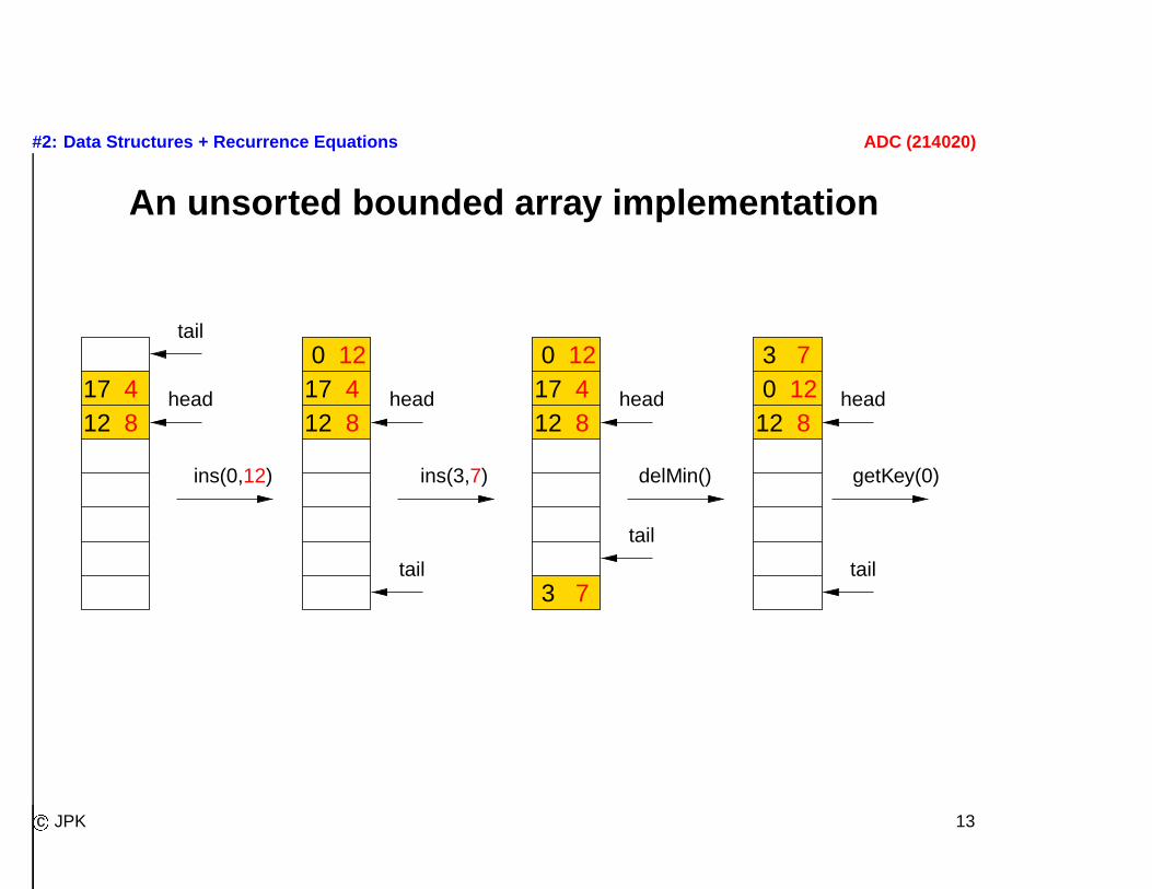
Binary trees (I)

� Lists organize data in a sequential order (a single successor)

– usually implied order in storage (e.g., sorted, FIFO, LIFO)– searching a specific data object requires traversing entire list– are there other ways to organize data?

� Consider a binary tree

– each data object has two pointers (left and right) to successive objects– this yields a storage structure like:

B

A

C

left right

6

12

225

key

leftchild of A child of A

right

parentof A and B

c� JPK 16


Binary trees (II)

� A binary tree is a set of nodes that is empty or else satisfies

– there is a single distinguished node called root– remaining nodes are divided into a left sub-tree and a right sub-tree– the left and right sub-tree of a leaf are empty

� in-degree of a node is 1 (except the root); its out-degree is maximally 2

� The level (or depth) of a node is its distance to the root

– the level of a tree is the maximum level of its leafs

balanced version is used as implementation of Java TreeMap class

c� JPK 17


Binary trees (III)

level 0

level 1

level 2

level 3

leve

l of

the

bina

ry tr

ee =

3

root

internal node

leaf

225

102

103 1056

4023

34

6

c� JPK 18


The benefits of binary trees

� Suppose you want to hold 30 data objects:

– Level 1 (root) holds 1 data object– Level 2 holds 2 data objects total: 3– Level 3 holds 4 data objects total: 7– Level 4 holds 8 data objects total: 15– Level 5 holds 16 data objects total: 31

� a data object can be traced in 5 steps (instead of 31) if stored handy

� Some facts about binary trees:

– there are at most � � nodes at level �

– a binary tree of level � contains at most �� nodes– a binary tree with� nodes has level at least ��

c� JPK 19


Listing the data objects of a binary tree (I)

225 225 225

225225225

102

103 1056

4023

34

6

102

103 1056

4023

34

6

102

103 1056

4023

34

6

102

103 1056

4023

34

6

102

103 1056

4023

34

6

102

103 1056

4023

34

6

Preorder traversal of a binary tree

c� JPK 20



225 225 225

225 225225

102

103 1056

4023

34

102

103 1056

4023

34

102

103 1056

4023

34

102

103 1056

4023

34

102

103 1056

4023

34

102

103 1056

4023

34

6 6 6

666

Inorder traversal of a binary tree

c� JPK 21



225 225 225

225 225225

102

103 1056

4023

34

102

103 1056

4023

34

102

103 1056

4023

34

102

103 1056

4023

34

102

103 1056

4023

34

102

103 1056

4023

34

6 6 6

666

Postorder traversal of a binary tree

c� JPK 22










c� JPK 23


Fibonacci numbers

� Consider the growth of a rabbit population, e.g.:

– suppose we have two rabbits, one of each sex– rabbits have bunnies once a month after they are 2 months old– they always give birth to twins, one of each sex– they never die and never stop propagating

� The # rabbits after � months is computed by:

� ��

� ��

� �� for� � �

� We thus obtain the sequence:

� 0 1 2 3 4 5 6 7 8 9 � � �

� �� 0 1 1 2 3 5 8 13 21 34 � � �c� JPK 24


A naive algorithm

int fibRec � int� � �

if � �� return� �

else return fibRec �� fibRec ��

� The # arithmetic steps � �� needed to compute fibRec � � � is:

� ��

� ��

� � � �� for� � �

� This is a recurrence equation!

� To decide the complexity class of fibRec we solve this equation(see also course on Combinatorics)

c� JPK 25


Applying the “substitution” method� � � � � � � �

� � � � � � � �

� � � �� for� � �

� Using induction we can prove (check!) that � ��

� How large is � � � � � � ? Can we give upper/lower bounds?

� It follows (by induction) that � �� for � � �

� But, this means that the complexity of fibRec is exponential:

fibRec � � ��

c� JPK 26


An iterative algorithm

int fibIter � int� � �

int curr � � � // current fib-numberif � �� curr � � �

int ppred � � � // pre-predecessorint pred � � � // predecessorfor ��

curr � pred� ppred �

ppred � pred � // shift ppredpred � curr � // shift pred

return curr �

� The # arithmetic steps � �� for � � � and 0 otherwise

� So, the complexity of fibIter is linear: fibIter � � ��

c� JPK 27


A matrix-exponentiation algorithm

� Is the fibIter algorithm optimal?

� No. The following matrix characterization helps:

� �

� �

� � � � � � � � � � � � � �

� � � � � � � � � � � � � ��

� � � � � � � � � � � � � � � �

� Thus, we can compute � � � � � � � � by matrix-powering:

� �� element (2,2) of� �

� ��

� Can we do matrix-powering efficiently? Luckily, we can!

c� JPK 28


Iterative squaring

int � � iterSq � int � �� int� � � //� � �

int � � Pow � � � // the zero-matrixif �� return� �

else if even �� Pow � iterSq ��

return Pow � Pow �

else � Pow � iterSq ��

return Pow � Pow ��

� The # arithmetic steps � � �� needed is:

� ��

� �� for� � �

� This yields a logarithmic complexity of iterSq: iterSq � � ��

c� JPK 29


Recall the practical implications

Maximal solvable input size if one operation takes 1 � second:

time allowed Recursive Iterative Matrix

1 msec 14 500 10� �

1 sec 28 � � � ��

1 min 37 � � � ��

1 hour 45 � � � ��

� Simplifying assumptions:

– only arithmetic operations were considered in the analysis– execution time is independent of the argument values

c� JPK 30


How to obtain recurrence equations from code?

� To obtain worst-case cost � � � � we inspect program fragments:

– for a sequence of blocks, add the individual costs– for an alternative of blocks, take the maximum of the alternatives– for a subroutine call take

�� where � �� is parameter size of call– for a recursive call, the cost is � �� where� �� is parameter size of call

we have applied this for the worst-case cost of Fibonacci programs already

� Note: obtaining recurrence equations for average-case analysis ismuch more difficult

– costs in case of alternative must be averaged (i.e., weighted sum)– if size of � �� and � �� vary, costs of subroutine/recursive calls must be

averaged

c� JPK 31










c� JPK 32


Some common recurrence equations

� Linear search: � � � � � � � � � � linear homogeneous

� Binary search: � � � � � � � � � � � non-linear homogeneous

� Bubblesort: � � � �� linear non-homogeneous

� Mergesort: � � � �� non-linear non-homogeneous

� Strassens’ matrix-multiplication: � � � ��

for linear (non-)homogeneous see course on Combinatorics

c� JPK 33


Solving recurrence equations

� For simple cases – occurring rarely here – closed-form solutionsexist, e.g.: see all course on Combinatorics

– � �� with � � � � � � has unique solution � ��

– � �� has unique solution � ��

– determining roots of characteristic equations– method of undetermined coefficients

� For the general case – occurring frequently here – no general solutiondoes exist

� Typical case: � � � ��

� � � � � � with � � � and �

– problem is divided into � similar problems of size� � each– non-recursive cost � �� to split problem or combine solutions of sub-problems

c� JPK 34


Technique 1: Substitution method

� The substitution method entails two steps:

1. guess the form of the solution (play with small input sizes)2. use induction to find the constants and to show that the solution works

� Example: � � � �� ; guess � � � ��

– proof obligation � �� for some appropriate � � �

– assuming it holds for � � � � � � � we do a check by substitution:

� ��

� (* removing floors makes it bigger *)

� ��

� (* some log-calculus using� � � � � � � � � � � � � � � � *)

� ��

� (* this follows immediately for � � � *)

� ��

– check base cases � � � � � � and � � � � � � and complete proof for � � �

c� JPK 35


Technique 2: The iteration method

Plug the recurrence back into itself until you recognize a pattern, e.g.:

� ��

� (* back-substitution *)� ��

� (* back-substitution again *)

� ��

� (* simplification *)

� ��

��

� ��

��

��

� ��

��

��

� ��

��

Assuming � � � � is constant, yields � � � ��

�

��

� � � � � �

� � � ��

this is easier to see using recursion trees

c� JPK 36


Technique 3: The recursion tree method (I)

� Visualize the back-substitution process as a tree, keeping track of

– the size of the remaining arguments in the recurrence– the nonrecursive costs

� very useful to obtain a good guess for substitution method

� The recurrence tree of � � � �� looks like:

..................

� ��

� ��

� �� remaining argumentfor recurrence

nonrecursive cost

c� JPK 37


Technique 3: The recursion tree method (II)

..................

..................

� ��

� ��

� ��

� ��

� ��

� � � � ��

� � � � � � leaves

��

� ��

� � � ��

� � � ��

sum overall levels

��

� �

� � �

cost perlevel

� � � ��

total cost forthe leafs

c� JPK 38


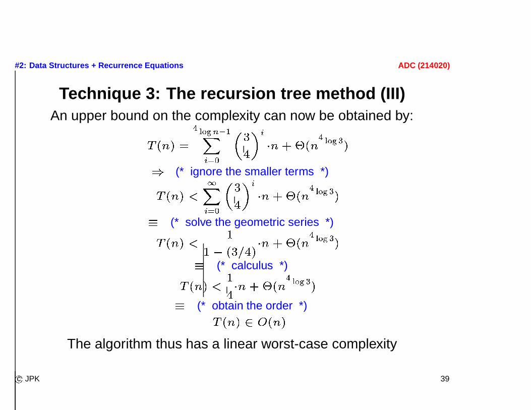
Technique 3: The recursion tree method (III)An upper bound on the complexity can now be obtained by:

� ��

��

� ��

��

�

� (* ignore the smaller terms *)

� ��

��

��

��

� � � � ��

� (* solve the geometric series *)

� ��

�

� � � � � � ��

� � � � ��

� (* calculus *)

� ��

��

� � � � ��

� (* obtain the order *)

� ��

The algorithm thus has a linear worst-case complexity

c� JPK 39


Technique 4: The Master theorem

� Consider: � � � ��

� � � � � � with � � � and �

– problem is divided into � similar problems of size� � each– non-recursive cost � �� to split problem or combine solutions of sub-problems– note that # leafs in the recursion tree is� � with � � � � � � � � � � �

� The Master theorem says:

if then1. � �� for some � � � � ��

2. � ��

3. � �� for some � � �

and � �� for some � � � � ��

� If none of the cases apply, the Master theorem gives no clue!

c� JPK 40


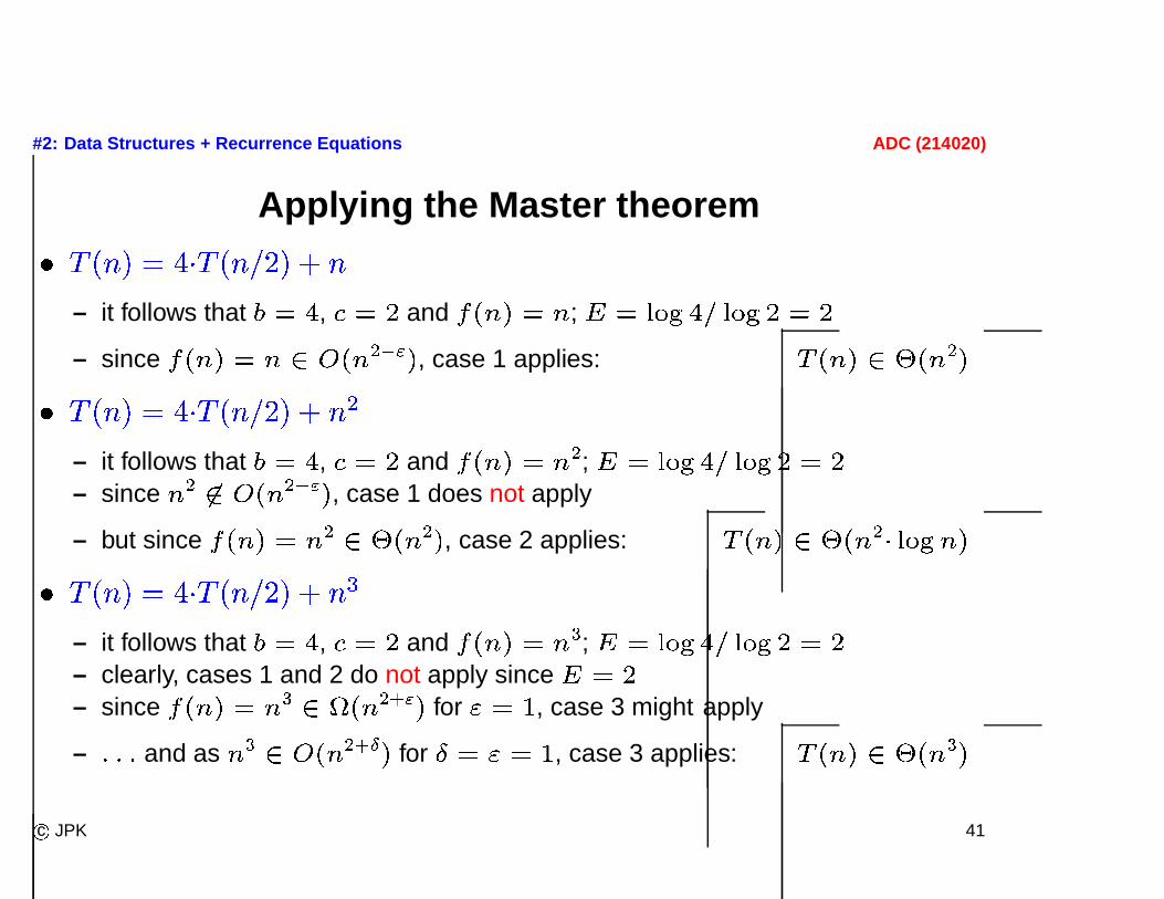
Applying the Master theorem

� � � � �� – it follows that � � � , � � � and � �� ; � � � � � � � � � � � � �

– since � �� , case 1 applies: � ��

� � � � ��

– it follows that � � � , � � � and � �� ; � � � � � � � � � � � � �

– since� �� , case 1 does not apply

– but since � �� , case 2 applies: � ��

� � � � ��

– it follows that � � � , � � � and � �� ; � � � � � � � � � � � � �

– clearly, cases 1 and 2 do not apply since � � �

– since � �� for � � � , case 3 might apply

– � � � and as� �� for � � � � � , case 3 applies: � ��

c� JPK 41


The Master theorem does not always apply

� � � � ��

– we have � � � , � � � and � �� ; � � �

– � � � �� since � ��

��

� case 1 of the Master theorem does not apply– � � � ��

� case 2 of the Master theorem does not apply– � �� since � ��

��

� case 3 of the Master theorem does not apply

� The Master theorem does not apply to this case at all!

� By substitution one obtains: � � � ��

c� JPK 42


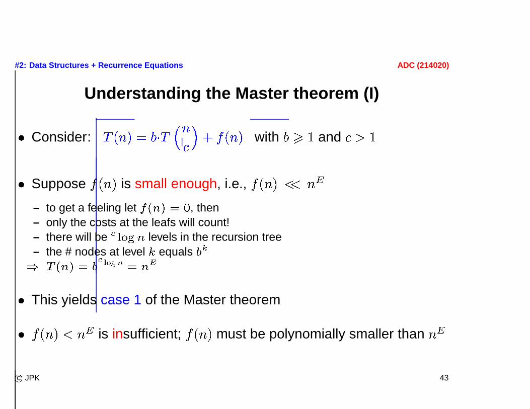
Understanding the Master theorem (I)


� � � � � � with � � � and �

� Suppose � � � � is small enough, i.e., � � � � � � ��

– to get a feeling let � �� , then– only the costs at the leafs will count!– there will be � � � � � levels in the recursion tree– the # nodes at level� equals ��

� � ��

� This yields case 1 of the Master theorem

� � � � � � �� is insufficient; � � � � must be polynomially smaller than ��

c� JPK 43


Understanding the Master theorem (II)


� � � � � � with � � � and �

� Suppose � � � � is large enough, i.e., � � � � � �

– if � �� is large enough, it will exceed � � � ��

– for instance � �� unless � � � �


� If � � � � and �� grow equally fast, the depth of the tree is important

– this perfect balance is what one wants to achieve with divide-and-conqueralgorithms!


c� JPK 44


Recurrence equations for some well-known algorithms

� Strassens’ matrix-multiplication: � � � ��

– we have� � � � � � �� is dominated by � ��

– case 1 of Master theorem applies and yields � ��

� Mergesort: � � � ��

– data is divided into equal-sized halves– and merging the sorted halves takes then � �� – � � � � � , but � ��

� � � , so case 1 does not apply

– but � �� , so by case 2 we obtain � �� c� JPK 45

Elementary Data Structures and Recurrence Equationsfmt.cs.utwente.nl/courses/adc/lec2.pdfRecurrence...

Documents

Transcript of Elementary Data Structures and Recurrence Equationsfmt.cs.utwente.nl/courses/adc/lec2.pdfRecurrence...