Electroactive Polymer Composites: Microscopic and ...
97
Electroactive Polymer Composites: Microscopic and Macroscopic Stability Thesis submitted in partial fulfillment of the requirements for the degree of ”DOCTOR OF PHILOSOPHY” by Stephan Rudykh Submitted to the Senate of Ben-Gurion University of the Negev 2012 Beer-Sheva
Transcript of Electroactive Polymer Composites: Microscopic and ...

Electroactive Polymer Composites:
Microscopic and Macroscopic Stability
Thesis submitted in partial fulfillment
of the requirements for the degree of
”DOCTOR OF PHILOSOPHY”
by
Stephan Rudykh
Submitted to the Senate of
Ben-Gurion University of the Negev
2012
Beer-Sheva

Electroactive Polymer Composites:
Microscopic and Macroscopic Stability
Thesis submitted in partial fulfillment
of the requirements for the degree of
”DOCTOR OF PHILOSOPHY”
by
Stephan Rudykh
Submitted to the Senate of
Ben-Gurion University of the Negev
Approved by the advisor
Approved by the Dean of the Kreitman School of Advanced Graduate Studies
2012
Beer-Sheva

This work was carried out under the supervision of
Professor Gal deBotton
Department of Mechanical Engineering,
Ben-Gurion University of the Negev,
Beer-Sheva, Israel
iii

Acknowledgments
Now, when the mysterious journey is nearing its end and the mist of terra incognita has
been scattered, revealing the beautiful detailed picture, there comes the time to thank
those who stood behind me supporting and encouraging.
I am in deep debt to my parents, Ludmila and Alexander. They made many sacrifices
so that I may pursue my education in the cruel times of the 1990’s in Russia. To my
deep sorrow, my father will not see the fruits of my work; he passed away just a few
months ago.
I would like to thank my lovely wife Anastasia and our daughters Anna and Daria. I
truly love you much more than this thesis, even though you may not believe so.
I would like to thank my advisor Prof. Gal deBotton - you have been like a father
for me in the scientific world, introducing me to the mystery of mechanics (I recall
the first lesson you gave me standing by the ”historical” board and writing the basics
of continuum mechanics...). Together we overcame the moments of desperation and
celebrated the excitements of new discoveries... I have already started missing those
days. I am sincerely grateful for all that I have learned from you and for you setting an
example with your inexhaustible scientific curiosity. Gal, thank you!
I was lucky to get the chance of working with Prof. Kaushik Bhattacharya who advised
me during my visit at Caltech. The semester I spent there was very special and provided
me with an important experience of working in Prof. Bhattacharya’s leading research
group. We discussed many ideas and I believe that pursuing all of them would have led
me to write several more theses. Truly, each discussion we had enriched and inspired
me in a unique way.
Finally, I thank Prof. Katia Bertoldi for fruitful discussions of various problems on
instabilities over the years via e-mails. At the very final stage of my study, I got the
chance of working with Prof. Bertoldi in Harvard University, thanks to the financial
support of the BSF Prof. Rahamimoff Award for Young Scientists. I thank Prof.
Bertoldi for the kind invitation and the opportunity to be a part of the outstanding
solid mechanics group.
From Beer-Sheva to Pasadena... on to Cambridge and back to Beer-Sheva, with the
help of all the good people along the way - here I am to submit the manuscript!
iv

Contents
Abstract 1
Chapter 1. Introduction 2
1.1. Motivation . . . . . . . . . . . . . . . . . . . . . . . . . . . . . . . . . . . 2
1.2. General Theoretical Background . . . . . . . . . . . . . . . . . . . . . . . 6
Chapter 2. Macroscopic Stability of Fiber Composites 11
2.1. Theory . . . . . . . . . . . . . . . . . . . . . . . . . . . . . . . . . . . . . 11
2.2. Fiber Reinforced Composites . . . . . . . . . . . . . . . . . . . . . . . . . 14
2.3. Finite Element Simulation . . . . . . . . . . . . . . . . . . . . . . . . . . 20
2.4. Applications . . . . . . . . . . . . . . . . . . . . . . . . . . . . . . . . . . 24
2.5. Conclusions . . . . . . . . . . . . . . . . . . . . . . . . . . . . . . . . . . 34
Chapter 3. Macroscopic Instabilities in Anisotropic Soft Dielectrics 36
3.1. Theory . . . . . . . . . . . . . . . . . . . . . . . . . . . . . . . . . . . . . 36
3.2. Applications to Soft Dielectric Laminates. . . . . . . . . . . . . . . . . . 37
Chapter 4. Microscopic Instabilities in EAPs 47
4.1. Theory. . . . . . . . . . . . . . . . . . . . . . . . . . . . . . . . . . . . . 47
4.2. Examples. . . . . . . . . . . . . . . . . . . . . . . . . . . . . . . . . . . . 53
4.3. Concluding Remarks . . . . . . . . . . . . . . . . . . . . . . . . . . . . . 67
Chapter 5. Thick-Wall EAP Balloon 68
Conclusions 73
Appendix A. Kinematic tensors of the TI invariants 75
Appendix B. Kinematic tensors of the electromechanical invariants 76
v

Appendix C. R-Matrix of the electromechanical instability analysis 77
Bibliography . . . . . . . . . . . . . . . . . . . . . . . . . . . . . . . . . . . 78
vi

List of Figures
1. A planar EAP actuator. . . . . . . . . . . . . . . . . . . . . . . . . . . . . . 2
2. The unstable domains of layered soft dielectric subjected to an electric excitation and
pre-stretch λ. A different types of instabilities and their domains are presented as
functions of the volume fraction of the stiffer phase c(f). . . . . . . . . . . . . . . 5
3. The kinematics of the incremental changes in the fields. . . . . . . . . . . . . . . 8
4. A scheme of a transversely isotropic composite and the associated physically motivated
invariants. . . . . . . . . . . . . . . . . . . . . . . . . . . . . . . . . . . . . 12
5. Schematic representation of the loading direction angle Θ. . . . . . . . . . . . . . 20
6. The hexagonal unit cell modeled in the finite element code COMSOL. . . . . . . . . 21
7. The dependence of the critical stretch ratio on the fiber volume fraction. The solid
curves correspond to fiber composites and the dashed curves to laminated composites.
The results of the numerical simulations are marked by triangles for k = 100 and
squares for k = 10. . . . . . . . . . . . . . . . . . . . . . . . . . . . . . . . . 25
8. The dependence of the critical stretch ratio on the loading direction. The solid,
dashed and short-dash curves correspond to composites with fiber to matrix shear
moduli ratio k = 50, 30 and 10, respectively. The simulation results are marked by
squares, triangles and circles for k = 50, 30 and 10, respectively. The thin continuous
curve shows the maximal loading angle Θm at which instability may occur. For all
curves c(f) = 0.5. . . . . . . . . . . . . . . . . . . . . . . . . . . . . . . . . . 26
9. The dependence of the maximal loading direction angle on the ratio between the shear
moduli. The solid, dashed and short-dash curves correspond to volume fractions of
the fiber c(f) = 0.1, 0.25 and 0.5, respectively. . . . . . . . . . . . . . . . . . . . 27
10. The critical stretch ratio as a function of the contrast between the phases shear moduli
for different loading directions. The continuous, dash and short-dashed curves corre-
spond to Θ = 0, π/16 and π/8, respectively. The results of the numerical simulation
are marked by squares, triangles and circles for Θ = 0, π/16 and π/8, respectively. . . 28
vii

11. The dependence of ω(G) and (ω(G))′ on the stretch ratio λ for the Gent composite with
Θ = 0, c(f) = 0.5, k = 100 and r = 1. The continuous curves correspond to ω(G)(λ)
for Jm = 0.1, 1, 10, 100 from right to left, while the dashed curves to (ω(G))′(λ). The
thin short-dash line corresponds to ω(H) for the neo-Hookean composite. The curve
crossings are marked by squares. The triangle indicates the critical stretch ratio for
these composites. . . . . . . . . . . . . . . . . . . . . . . . . . . . . . . . . 31
12. The dependence of the critical stretch ratio λc on the locking parameter Jm. The solid
line corresponds to shear moduli ratio k = 100, and the dashed curve to k = 50. The
dotted curve represents the lock-up stretch ratio. The numerical simulation results
are marked by squares and circles for k = 100 and 50, respectively. . . . . . . . . . 32
13. The dependence of the critical stretch ratio λc on the locking parameter Jm for k =
100. The solid, dashed and short-dashed curves correspond to Θ = 0, π/16 and π/8,
respectively. The results of the numerical simulations are marked by squares, triangles
and circles for Θ = 0, π/16 and π/8, respectively. The corresponding solutions for
the neo-Hookean composites are marked by dashed thin lines. The locking curve is
the dotted one. The thin continuous curve represents the maximal loading angle for
which instabilities were detected. . . . . . . . . . . . . . . . . . . . . . . . . . 33
14. Electroactive layered composite subjected to electric excitation . . . . . . . . . . . 40
15. Bifurcation diagrams of layered materials with different lamination angles as functions
of the critical stretch ratio and electric displacement field. The volume fractions of
the stiffer phase is c(f) = 0.2 for (a) and (b) and c(f) = 0.8 for (c) and (d); the phase
constant ratios are k = t = 10. Figures (a) and (c) are for small lamination angles,
and figures (b) and (d) are for large lamination angles. . . . . . . . . . . . . . . . 41
16. Bifurcation diagrams of layered materials as functions of the critical stretch ratio and
the lamination angle at different levels of electric excitations. The volume fraction
of the stiffer phase is c(f) = 0.2, the shear moduli ratio is k = 10, and the dielectric
constants ratio is t = 10. . . . . . . . . . . . . . . . . . . . . . . . . . . . . . 42
17. The failure surfaces of layered composites with different lamination angles as functions
of the critical stretch ratio and volume fraction of the stiffer phase subjected to a fixed
electrostatic excitation Dn = 4.0. The shear moduli ratio is k = 10, and the dielectric
constants ratio is t = 10. . . . . . . . . . . . . . . . . . . . . . . . . . . . . . 44
18. Electroactive layered composite subjected to electric excitation . . . . . . . . . . . 45
19. Bifurcation diagrams of layered materials subjected to aligned stretch and electrostatic
excitation at different angles as functions of the critical stretch ratio and electric
displacement. The volume fraction of the stiff phase is c(f) = 0.8 and the contrasts
between the elastic and dielectric moduli are k = t = 10. . . . . . . . . . . . . . 46
viii

20. Electroactive layered composite subjected to electric excitation. . . . . . . . . . . . 48
21. The unit cell of the layered media. . . . . . . . . . . . . . . . . . . . . . . . . 49
22. The dependence of the critical stretch ratio on the electric field for layered composites
with Θ = 0. The volume fractions of the stiffer phase are c(f) = 0.05, 0.1, 0.2, 0.5
(magenta, blue, green and red curves, respectively). The contrasts in the properties
of the phases are k = t = 10. The continuous and dashed curves represent the onset
of macroscopic and microscopic instabilities, respectively. . . . . . . . . . . . . . . 55
23. The dependence of the critical electric field on the dimensionless wave number k1h
for composite with volume fraction of the stiffer phase c(f) = 0.5. The contrasts in
the properties of the phases are k = t = 10. The continuous curves correspond to
those loading parameters for which the first instability occurs at k1h = 0 whereas the
dashed curves are for those parameters where the instability occurs at a finite wave
length. . . . . . . . . . . . . . . . . . . . . . . . . . . . . . . . . . . . . . 57
24. Bifurcation diagrams of layered composites with contrasts in the phase properties
k = t = 50 as functions of the critical stretch ratio and the referential electric field.
The volume fractions of the stiffer phase c(f) = 0.05, 0.1, 0.2 and 0.5 (magenta, blue,
green and red curves, respectively). The continuous and dashed curves represent the
onset of macroscopic and microscopic instabilities, respectively. . . . . . . . . . . . 58
25. Bifurcation diagrams of layered composites with volume fractions of the stiffer phase
c(f) = 0.05, 0.1, 0.2 and 0.5 (magenta, blue, green and red curves, respectively)
as functions of the electric field E and electric displacement D. The continuous
and dashed curves represent the onset of macroscopic and microscopic instabilities,
respectively. . . . . . . . . . . . . . . . . . . . . . . . . . . . . . . . . . . . 59
26. Bifurcation diagrams of layered composites with volume fractions of the stiffer phase
c(f) = 0.05, 0.1, 0.2 and 0.5 (magenta, blue, green and red curves, respectively)
as functions of the longitudinal mean stress and the referential electric field. The
continuous and dashed curves represent the onset of macroscopic and microscopic
instabilities, respectively. . . . . . . . . . . . . . . . . . . . . . . . . . . . . . 60
27. The longitudinal stresses as functions of applied electric field of layered composites
with volume fraction of the stiffer phase c(f) = 0.5. The dotted, continuous and
dashed curves correspond to the stresses along the equilibrium path λ = 2, onset of
macroscopic and microscopic instabilities, respectively. The red curves represent the
stresses in the stiffer phase and the blue ones correspond to the stresses in the softer
phase. The black curves represent the mean stresses. . . . . . . . . . . . . . . . . 61
ix

28. The failure surfaces of layered composites as functions of the critical stretch ratio and
volume fraction of the stiffer phase. The contrasts in the properties of the phases are
k = t = 10. The red, green, magenta and blue curves correspond to E = 1.0, 1.6, 1.8
and 2.0, respectively. The continuous and dashed curves correspond to the onset of
the macroscopic and microscopic instabilities, respectively. The dotted curves separate
the unified unstable domains according to the instability mode associated with each
part. . . . . . . . . . . . . . . . . . . . . . . . . . . . . . . . . . . . . . . 62
29. The macroscopic failure surfaces of layered composites as functions of the stretch ratio
and the volume fraction of the stiffer phase. The contrasts in the properties of the
phases are k = t = 10. (a) - E = 1.0; (b) - E = 2.0 . . . . . . . . . . . . . . . . . 63
30. Failure surfaces of layered composites with Θ = 0 as functions of the stretch ratio and
volume fraction of the stiffer phase. The contrasts in the properties of the phases are
k = t = 10. The blue, red, black, green, magenta and purple curves correspond to
E = 1.9, 1.925, 1.95, 1.975, 2.0 and 2.025, respectively. . . . . . . . . . . . . . . . 64
31. The bifurcation diagrams of layered composites with different lamination angles as
function of the critical stretch ratio and the referential electric field. The volume
fraction of the stiffer phase is c(f) = 0.2 and the contrasts in the properties of the
phases are k = t = 10. (a) - small angles; (b) - large angles . . . . . . . . . . . . . 65
32. Bifurcation diagrams as functions of the stretch ratio and lamination angle. The
contrasts in properties of the phases are k = t = 10. . . . . . . . . . . . . . . . . 66
33. Deformation of a thick-wall balloon due to (a) inflation pressure and (b) electrostatic
excitation. The continuous and dashed curves correspond to Ogden and neo-Hookean
materials, respectively. . . . . . . . . . . . . . . . . . . . . . . . . . . . . . . 69
34. The deformations of balloons with different wall thicknesses as functions of the pres-
sure with fixed electric excitation. The dashed curve corresponds to the thin-wall
approximation (210). . . . . . . . . . . . . . . . . . . . . . . . . . . . . . . . 70
35. Actuation cycles of a dielectric balloon subjected to (a) inflation pressure and (b)
electrostatic excitation. . . . . . . . . . . . . . . . . . . . . . . . . . . . . . . 71
36. Pumping cycle of a dielectric balloon subjected to (a) inflation pressure and (b) elec-
trostatic excitation. . . . . . . . . . . . . . . . . . . . . . . . . . . . . . . . 72
x

Abstract
This thesis is concerned with theoretical aspects of instability development in heteroge-
neous dielectrics capable of large elastic deformations. A general instability criterion is
introduced to identify the limiting case of large-scale or macroscopic instabilities. Multi-
scale instabilities are determined by application of Bloch-Floquet technique to periodic
media. I begin with the purely mechanical case, and develop a criterion for the onset of
macroscopic instabilities in spatial composites with randomly distributed aligned fibers.
This states that the composite fails when the compression in the fiber direction reaches
a certain value given by a compact explicit expression. The results are confirmed by 3-D
finite element simulations for which a unique algorithm of instability onset identification
was developed.
Motivated by experiments and possible applications, a coupled electromechanical
analysis is conducted in terms of the physically relevant referential electric field as
well as in terms of the electric displacement. In terms of the former, a closed form
solution is derived for the macroscopic instabilities for the class of layered neo-Hookean
dielectrics. A criterion for the onset of electromechanical multiscale instabilities for the
layered composites with anisotropic phases is formulated too. These reveal the essential
influence of the microstructure on the onset of instabilities. Specifically, it is found that
(i) macroscopic instabilities dominate at moderate volume fractions of the stiffer
phase
(ii) interface instabilities appear at small volume fractions of the stiffer phase
(iii) instabilities of finite length scales comparable with the microstructure size, take
place at large volume fractions of the stiffer phase
The instabilities of type (iii) do not appear in the purely mechanical case and dominate
in the region of high stiffer phase volume fractions. The unstable domains evolve with
an increase of the electric field: expand, meet, unite and create new unstable domains
in a certain way.
Finally, an exact solution for thick spherical balloons subjected to inflating pressure
and electric excitation is derived and possible applications of the observed instability
phenomenon to micro-pumps is discussed.
1

Chapter 1
Introduction
1.1 Motivation
Electroactive polymers (EAPs) respond to external electric stimuli by changing their
size and shape. These soft dielectrics can be utilized to convert electrical energy into
mechanical work. As promising actuators, EAPs offer the benefits of light weight, short
response time and simple principle of work. An example of an EAP planar actuator is
shown in Fig. 1. The top and bottom surfaces are covered with compliant electrodes
that enable to induce an electric field through the material thickness. The so-called
Maxwell stresses induced by the electrostatic field act to reduce the material thickness
and thanks to the Poisson’s effect lead to in-plane extension of the material.
Elastomer
Compliant Electrodes
V
Undeformed Configuration Deformed Configuration(by Maxwell Stresses)
Fig. 1. A planar EAP actuator.
The field of EAPs has been intensively studied experimentally and theoretically in
the last decade and consequently have now become feasible to use as actuators (Pel-
rine et al., 2000; Bar-Cohen, 2001; Bhattacharya et al., 2001; Lacour et al., 2004; Carpi
and DeRossi, 2005; Carpi et al., 2007; O’Halloran et al., 2008; Stoyanov et al., 2011).
However, in spite of the significant progress, these materials are limited by the ex-
tremely strong electric fields they require for meaningful actuation. The reason for this
is the poor electromechanical coupling in typical polymers which have a limited ratio
of dielectric to elastic modulus. One approach to tackle this issue is to make electroac-
2

tive polymer composites (EAPC) by combining an elastomer with a high dielectric or
even conductive material (Zhang et al., 2002; Huang et al., 2004). This approach has
shown to be promising in several experiments (e.g., Huang and Zhang, 2004; Stoyanov
et al., 2011). Moreover, theoretical estimations (deBotton et al., 2007; Tian et al., 2012;
Rudykh et al., 2011) have shown that the experimental results are only a beginning, and
proper optimization of microstructures can lead to orders of magnitude improvement in
the electromechanical coupling.
An important aspect of the EAPC behavior concerns the possible development of in-
stabilities under certain electromechanical loading conditions. On one hand, instabilities
are commonly considered as negative phenomena associated with failure. On the other,
they can be viewed as a trigger for giant deformations of specific structures (Mocken-
sturm and Goulbourne, 2006; Rudykh et al., 2012b) or for manipulating microstructural
patterns in composite media (Singamaneni et al., 2009, for purely mechanical case). The
latter can be utilized for controlling material properties, with a large variety of possible
applications such as wave guide filtering (Gei et al., 2010).
Before tackling the more complex problem of coupled instabilities, herein the corre-
sponding purely mechanical problem is investigated. A fundamental study of mechanical
instabilities in composite materials was performed by Biot (1965), who developed a the-
ory for pre-stressed rubber-like solids in finite deformation. Rosen (1965) estimated
the compressive strength of fiber composites based on a beam theory. A general dis-
cussion concerning the bifurcation phenomena was provided by Hill and Hutchinson
(1975). Among the methods that take into account imperfections in fiber composites
one should mention the works of Budiansky (1983); Fleck (1997) and Merodio and Pence
(2001). The problem of a localized failure at the free surface of orthotropic materials
was examined by deBotton and Schulgasser (1996).
In composite materials, bifurcations may occur at a scale which is significantly
smaller than the size of the specimen. Triantafyllidis and Maker (1985) determined the
onset of purely mechanical instabilities in periodic layered media at such microscopic
levels, as well as at the macroscopic level. These investigators noted that macroscopic
instabilities that occur at a scale significantly larger than the scale of the microstructure
can be detected with the help of the homogenized tensor of elastic moduli. The onset
of these instabilities is associated with loss of ellipticity of the homogenized governing
equations. Detecting instabilities at a smaller scale requires the use of more complicated
techniques such as Bloch wave analysis (e.g., Kittel, 2004). Geymonat et al. (1993)
showed that Floquet theorem or Bloch wave technique can be applied for analyzing the
characteristic unit cell and predicting the onset of failures at any scale.
Nestorovic and Triantafyllidis (2004) determined loss of stability in 2-D layered com-
3

posites subjected to combined shear and compression. Periodic fiber composites sub-
jected to in-plane transverse deformation were numerically examined by Triantafyllidis
et al. (2006) for the case of neo-Hookean phases, and by Bertoldi and Boyce (2008) for
both neo-Hookean and Gent phases. Michel et al. (2007) compared numerical results for
the transverse behavior and loss of stability of periodic porous fiber composites with cor-
responding predictions of the variational estimate of Lopez-Pamies and Ponte Castaneda
(2004). The 2-D finite element (FE) analyses performed in the above mentioned works
did not cover instabilities due to compression along the fibers. In this work the onset of
this important mode of failure (e.g., Merodio and Ogden, 2002; Qiu and Pence, 1997) is
analyzed. A numerical analysis requires examination of 3-D models subjected to finite-
strain loading conditions. Accordingly, in contrast to the FE models used in previous
works, a 3-D model is developed and appropriate techniques are applied for determining
the onset of instabilities. Complementary to the numerical study, analytical predictions
for the onset of stability loss in composites with random distribution of aligned fibers
are determined. An important result of the study of the purely mechanical stability is
that the onset of macroscopic instability occurs whenever the compression in the fiber
direction reaches the stretch ratio
λn =
(1− µ
µ
)1/3
, (1)
where µ and µ are the out-of-plane and isochoric shear moduli of the composite. This
result was reported by deBotton (2008); Rudykh and deBotton (2012) and Agoras et al.
(2009b). Additionally, a new upper estimate for composites with Gent phases is intro-
duced. Differently from the results of Agoras et al. (2009b), an analytical closed form
expression is derived for the onset of instabilities in these composites.
Towards the treatment of the coupled electromechanical problem, I recall that the
basic theory of elastic dielectrics that accounts for the Maxwell electrostatic stresses was
introduced by Toupin (1956). More recently, McMeeking and Landis (2005), Dorfmann
and Ogden (2005) and Suo et al. (2008) extended this theory.
While purely mechanical instabilities have been studied intensively for decades, the
coupled instability is a new topic and no results were available until lately. Electrome-
chanical instabilities such as pull-in instabilities (Plante and Dubowsky, 2006), electrical
breakdown (Kofod et al., 2003; Stoyanov et al., 2011) and failure mechanisms at high
electric fields (Wang et al., 2011) in homogeneous electroactive materials were studied
experimentally. Liu et al. (2010) and Molberg et al. (2010) investigated the electrical
breakdown of EAP composites with random distribution of high dielectric particles.
Dorfmann and Ogden (2010) examined the problem of surface instabilities account-
ing for the incremental governing equations in isotropic dielectrics. Recently, Bertoldi
4

0 . 0 0 . 2 0 . 4 0 . 6 0 . 8 1 . 00 . 6
0 . 8
1 . 0
1 . 2
1 . 4
1 . 6
1 . 8
2 . 0E = 1 . 6 F i n i t e s c a l e i n s t a b i l i t i e s
k 1 h ~ 2 �( f i n i t e w a v e s )
S t a b l e D o m a i nI n t e r f a c e i n s t a b i l i t i e s k 1 h ~ 2 �� ( s h o r t w a v e s )
c ( f )
�
M a c r o s c o p i c i n s t a b i l i t i e s k 1 h ~ 0 �( l o n g w a v e s )
Fig. 2. The unstable domains of layered soft dielectric subjected to an electric excitation and pre-stretch λ. A different types of instabilities and their domains are presented as functions of the volumefraction of the stiffer phase c(f).
and Gei (2011) investigated instabilities in soft layered dielectrics with isotropic phases
in which the electric field is perpendicular to the layers and pre-stretch is applied along
the layers. It is worth reminding that for this configuration no enhancement of the
actuation due to heterogeneity can be achieved. In contrast to this, when one of the
phases is anisotropic a significant enhancement of up to two orders of magnitude can
be achieved (Tevet-Deree, 2008; Tian et al., 2012; Rudykh et al., 2011). This motivates
the investigation of the onset of instabilities in composites with anisotropic phases.
In the context of macroscopic instabilities, an extension of the work by Dorfmann
and Ogden (2010) to a general class of multiphase electroactive materials undergoing
large deformations is introduced. Herein, a general criterion for the onset of macroscopic
instability in anisotropic media for planar problems is developed.
Previous works (Dorfmann and Ogden, 2010; Bertoldi and Gei, 2011) involve the
electrical displacement as a primary variable. However, this mathematically convenient
approach demands from experimentalists to control surface charge. This task is rather
difficult and hardly likely to be adopted in future since in potential applications the
electric excitation is induced by voltage. Contrary to the above mentioned works, in
this study the analysis is conducted in terms of a comprehensive variable, namely the
referential electric field. The latter is directly related to the applied voltage ∆φ as E0 =
∆φ/d, where d is the distance between the electrodes in the undeformed configuration.
Beyond the practicality of the proposed concept, it reveals a few important aspects of
5

the behavior that are hard to capture by making use of the “surface charge” formulation.
Among these are the identification of critical morphologies for which the composite
becomes extremely unstable and determination of critical voltages above which the
medium loses its stability or, conversely, becomes stable. The major result of this study
may be summarized as follow: in layered electroactive media three primary modes of
instabilities can be distinguished. These are characterized by different wavelengths and
are allocated depending on the composite morphology. These modes are shown in Fig. 2
as functions of the pre-stretch λ and the volume fraction of the stiffer phase c(f).
(i) The first mode is characterized by instabilities at long wavelengths and dominates
at moderate volume fractions of the stiffer phase.
(ii) The second mode corresponds to instabilities at short wavelengths and appears at
low volume fractions of the stiffer phase.
(iii) The third mode represents instabilities at finite wavelengths comparable with the
microstructure characteristic size. The instabilities of this mode occur at high
volume fractions of the stiffer phase.
The unstable domains evolve with the applied electric field: expand, meet, unite and
create new unstable domains in a certain way such that the overall unstable domain
extends with an increase of the electric field. The morphology and geometry of the
microstructure significantly impact the onset of instabilities.
The results for the purely mechanical instabilities in fiber composites are summarized
in Chapter 2 and are based on the work of Rudykh and deBotton (2012). The analysis of
electromechanical instabilities in anisotropic soft dielectrics with application to layered
media (Rudykh and deBotton, 2011) is presented in Chapter 3. The results related
to multiscale electromechanical instabilities (Rudykh et al., 2012a) are summarized in
Chapter 4. An example of usage of the electromechanical instability phenomenon with
possible application for micro-pumps is demonstrated in Chapter 5. The results of the
last chapter rely on the work of Rudykh et al. (2012b).
1.2 General Theoretical Background
The Cartesian position vector of a material point in a reference configuration of a body
B0 is X, and its position vector in the deformed configuration B is x. The deformation
of the body is characterized by the mapping
x = χ(X). (2)
6

The deformation gradient is
F =∂χ(X)
∂X. (3)
It is assumed that the deformation is invertible and hence F is non-singular, accordingly
J ≡ det F 6= 0. (4)
Physically, J is the volume ratio between the volumes of an element in the deformed
and the reference configurations, and hence J = dvdV
> 0.
The differential operators in the reference configuration are denoted Div(•) and
Curl(•) and the corresponding operators in the current configuration are div(•) and
curl(•), respectively. The deformation is assumed to be quasi-static and no magnetic
field is assumed to be present. Consequently, Maxwell equations reduce to
divD = 0, curlE = 0. (5)
Here D is the electric displacement and E is the electric field in the current configuration.
Following Dorfmann and Ogden (2005), these equations can be rewritten in terms
of the referential electric field E0 = FTE and the referential electric displacement D0 =
JF−1D as
DivD0 = 0 and CurlE0 = 0. (6)
In the absence of body forces the equilibrium equation is
DivP = 0, (7)
where P is the total nominal stress tensor which is the sum of purely elastic and elec-
trostatically induced Maxwell stresses. The corresponding total true or Cauchy stress
tensor is related to the nominal stress tensor via the relation σ = J−1PFT .
Consider hyperelastic dielectrics whose behaviors are characterized by a scalar-valued
energy-density function Ψ(F,E0)
P =∂Ψ(F,E0)
∂Fand D0 = −∂Ψ(F,E0)
∂E0(8)
For an incompressible material the nominal stress tensor is
P =∂Ψ(F,E0)
∂F− pF−T , (9)
where p is an arbitrary pressure.
The boundary conditions are
[[u]] = 0, [[σ]] · n = 0, [[D]] · n = 0 and n× [[E]] = 0, (10)
7

0
F
Xx
1e 2e
3e
Referenceconfiguration
Currentconfiguration
0 0 0
ijkl ijk ij, ,A G E
ijkl ijk ij, ,A G E
Fig. 3. The kinematics of the incremental changes in the fields.
where u = x−X is the displacement vector and n = JF−T N is normal to the boundary
at the current configuration. The notation [[•]] ≡ (•)+−(•)− denotes the jump between
the fields in the material and surrounding across the boundary. In general, the body
may be surrounded by another material as in the case of a multiphase medium, or by
vacuum in the case of an isolated body.
The incremental governing equations are (Dorfmann and Ogden, 2010)
DivP = 0, DivD0 = 0 and CurlE0 = 0. (11)
where P, D0 and E0 are infinitesimal changes in the nominal stress, electric displacement
and electrical field, respectively. The linearized constitutive equations are provided via
the electroelastic moduli tensors
A0iαkβ =
∂2Ψ
∂Fiα∂Fkβ, G0
iαβ =∂2Ψ
∂Fiα∂E0β
and E0αβ =
∂2Ψ
∂E0α∂E
0β
, (12)
namely,
Pij = A0ijklFkl + G0
ijkE0k and − D0
i = G0jkiFjk + E0
ijE0j . (13)
For an incompressible material the linearized constitutive relations are
Pij = A0ijklFkl + G0
ijkE0k − pF−Tij + pF−1
jk FklF−1li , −D0
i = G0jkiFjk + E0
ijE0j , (14)
where p is an incremental change in pressure. Consider the current configuration as a
new reference configuration (see Fig. 3). Recall that F = (grad v)F, where vi = xi is
8

an incremental displacement. The incremental “push-forward” of P, E0 and D0 to the
current configuration are
T = J−1PFT , D = J−1FD0 and E = F−T E0. (15)
In terms of these increments, the linearized constitutive equations are
Tij = Aijklvk,l + GijkEk − pδij + pvj,i, −Di = Gjkivj,k + EijEj, (16)
where
Aijkl = J−1FjαFlβA0iαkβ, Gijk = J−1FjαFkβG0
iαβ, Eij = J−1FiαFjβE0αβ. (17)
The electroelastic moduli possess the symmetries
Aijkl = Aklij, Gijk = Gjik and Eij = Eji. (18)
The incremental governing equations (11) become
divT = 0, divD = 0 and curlE = 0. (19)
Upon substitution of the linearized relations (16) in (19), the following equations are
obtained
Aijklvk,lj + GijkEk,j − p,i = 0 and Gjkivj,ki + EijEj,i = 0. (20)
The boundary conditions of the incremental fields are
[[v]] = 0, [[T]] · n = 0, [[D]] · n = 0 and n× [[E]] = 0. (21)
While Eqs. (5), (7) and (8) together with boundary conditions (10) define the electrome-
chanical boundary value problem, possible bifurcations of the solution are analyzed by
making use of the incremental Eqs. (19) together with boundary conditions (21).
Alternatively, an energy density function Φ can be written in terms of independent
variables F and D0 (Dorfmann and Ogden, 2005) such that
P =∂Φ(F,D0)
∂Fand E0 =
∂Φ(F,D0)
∂D0. (22)
Then the linearized constitutive equations are
Pij = A0ijklFkl +K0
ijkD0k and E0
i = K0jkiFjk +D0
ijD0j , (23)
where
K0iαβ =
∂2Φ
∂Fiα∂D0β
and D0αβ =
∂2Φ
∂D0α∂D
0β
. (24)
9
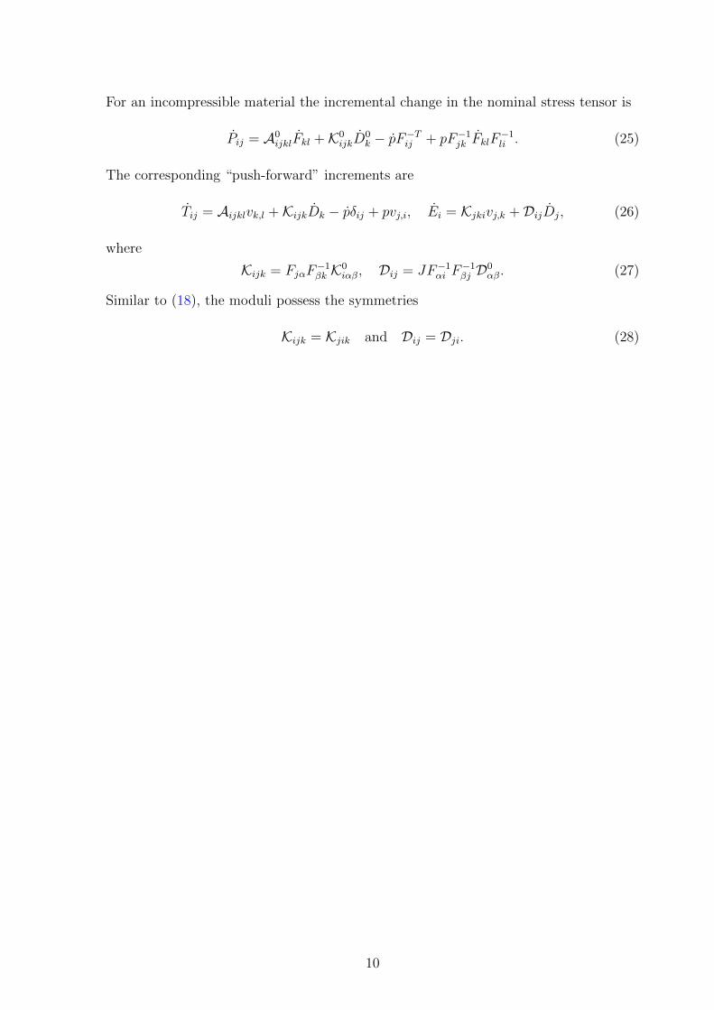
For an incompressible material the incremental change in the nominal stress tensor is
Pij = A0ijklFkl +K0
ijkD0k − pF−Tij + pF−1
jk FklF−1li . (25)
The corresponding “push-forward” increments are
Tij = Aijklvk,l +KijkDk − pδij + pvj,i, Ei = Kjkivj,k +DijDj, (26)
where
Kijk = FjαF−1βk K
0iαβ, Dij = JF−1
αi F−1βj D
0αβ. (27)
Similar to (18), the moduli possess the symmetries
Kijk = Kjik and Dij = Dji. (28)
10

Chapter 2
Macroscopic Stability of Fiber Composites
Composite materials are widely used in various engineering areas. Therefore character-
ization of their properties is of importance for both engineering applications and theo-
retical development of methods that can reduce the need for high-cost experiments. An
important and hard to predict characteristic is the one associated with loss of stability,
also referred to as “local buckling”. This phenomenon is mostly considered as a failure
mode that should be predicted and avoided. However, in some cases, such as in “snap-
through” mechanisms this phenomenon can be used for our benefit (e.g., O’Halloran
et al., 2008). In this chapter, only purely mechanical instabilities are considered.
2.1 Theory
In the purely mechanical case the energy-density function Ψ of an isotropic material
can be expressed in terms of the three invariants of the Cauchy-Green strain tensor
C ≡ FTF. It is common to express these invariants in the form
I1 = TrC, I2 =1
2(I2
1 − Tr(C2)), I3 = det C. (29)
A widely used isotropic and incompressible model that enables to capture the “lock-up”
effect of the molecular chain extension limit is the Gent (1996) model (e.g., Horgan
and Saccomandi (2002))
ΨG = −1
2µJm ln
(1− I1 − 3
Jm
). (30)
Here µ is the initial shear modulus and Jm is a dimensionless locking parameter corre-
sponding to the lock-up phenomenon such that in the limit (I1 − 3) → Jm, there is a
dramatic rise of the stresses and the material locks up. In the limit Jm →∞ this model
is reduced to the neo-Hookean model, namely
ΨH =µ
2
(I1 − 3
). (31)
The strain energy-density function of a transversely isotropic (TI) material, whose
preferred direction in the reference configuration is along the unit vector N, depends on
two additional invariants
I4 = N ·CN and I5 = N ·C2N. (32)
11
X1
X2
X3
γncosψγγnsinψγ
γp
λp
λp
λn
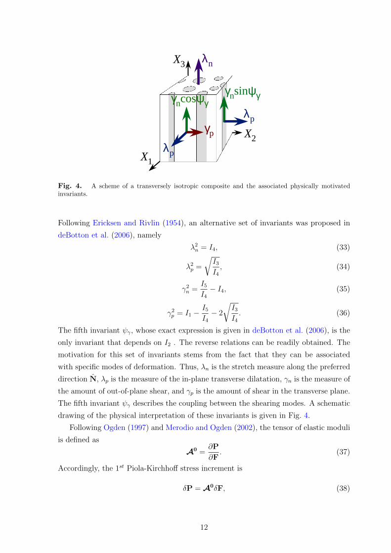
Fig. 4. A scheme of a transversely isotropic composite and the associated physically motivatedinvariants.
Following Ericksen and Rivlin (1954), an alternative set of invariants was proposed in
deBotton et al. (2006), namely
λ2n = I4, (33)
λ2p =
√I3
I4
, (34)
γ2n =
I5
I4
− I4, (35)
γ2p = I1 −
I5
I4
− 2
√I3
I4
. (36)
The fifth invariant ψγ, whose exact expression is given in deBotton et al. (2006), is the
only invariant that depends on I2 . The reverse relations can be readily obtained. The
motivation for this set of invariants stems from the fact that they can be associated
with specific modes of deformation. Thus, λn is the stretch measure along the preferred
direction N, λp is the measure of the in-plane transverse dilatation, γn is the measure of
the amount of out-of-plane shear, and γp is the amount of shear in the transverse plane.
The fifth invariant ψγ describes the coupling between the shearing modes. A schematic
drawing of the physical interpretation of these invariants is given in Fig. 4.
Following Ogden (1997) and Merodio and Ogden (2002), the tensor of elastic moduli
is defined as
A0 =∂P
∂F. (37)
Accordingly, the 1st Piola-Kirchhoff stress increment is
δP = A0δF, (38)
12

where δF is an infinitesimal variation in the deformation gradient from the current
configuration. If the deformation is homogeneous then A0iαjβ is independent of X and
the incremental equilibrium equation can be written in the form
A0iαjβ
∂2δχj∂Xα∂Xβ
= 0, (39)
where δχ is the incremental displacement associated with δF. For incompressible ma-
terials the equilibrium equation is
A0iαjβ
∂2δχj∂Xα∂Xβ
+∂δp
∂xi= 0, (40)
where δp is a pressure increment. Incompressibility implies zero divergence of the dis-
placement field, that is
∇ · δχ = 0. (41)
I seek a solution for Eq. (40) in the form of a standing plane wave, namely
δχ = vf(x · a), δp = qf(x · a), (42)
where v and a are two unit vectors. Function f represents the disturbance shape and
should be sufficiently continuously differentiable. To ensure the property the function
is chosen to be an exponential function
δχ = veia·x, δp = qeia·x. (43)
Note that for both forms of the solution, either for general form f or the exponential
form (43), the identical condition is derived. The incompressibility constraint Eq. (41)
leads to the requirement
a · v = 0. (44)
By application of the chain rule, the incremental equilibrium equations (40) can be
written in the form
Aipjq∂2δχj∂xp∂xq
+∂δp
∂xi= 0, (45)
where
Aipjq = J−1FpαFqβA0iαjβ. (46)
Substitution of Eq. (43) into Eq. (45) results in the equation
Qv + iqa = 0, (47)
where
Qij ≡ Apiqj apaq, (48)
13

is the acoustic tensor.
Finally, I note that the ellipticity condition implies that Qij vivj 6= 0 for all vectors a
and v such that a⊗ v 6= 0. However, since negative values of Qij vivj are not physical,
the strong ellipticity conditions can be written as
Qij vivj > 0. (49)
The unit vector v is the normal to a surface, in the deformed configuration, which is
referred to as a weak surface (e.g., Merodio and Ogden (2002)). Once the critical
deformation corresponding to the onset of ellipticity loss is achieved, the deformation
in the weak surface occurs along the direction of the vector a.
2.2 Fiber Reinforced Composites
The strain energy-density function of a n-phase composite is
Ψ(F,X) =n∑r=1
ϕ(r)(X)Ψ(r)(F), (50)
where
ϕ(r)(X) =
{1 if X ∈ B(r)
0 ,
0 otherwise,(51)
In Eq. (51) B(r)0 denotes the domain occupied by r-phase. The volume fraction of the
r-phase is
c(r) =
∫B0
ϕ(r)(X)dV. (52)
Following the works of Hill (1972) and Ogden (1974), I apply homogeneous boundary
conditions x = F0X on the boundary of the composite ∂B0, where F0 is a constant
matrix with det F0 > 0. It can be shown that F = F0 where
F =1
V
∫B0
F(X)dV, (53)
is the average deformation gradient. The average 1st Piola-Kirchhoff stress tensor is
P =1
V
∫B0
P(X)dV. (54)
By application of the principle of minimum energy, the effective strain energy-density
function is
Ψ(F) = infF∈K(F)
1
V
∫B0
Ψ(F, X)dV
, (55)
14

where K(F) ≡{
F | F =∂χ(X)
∂X, X ∈ B0; χ(X) = FX, X ∈ ∂B0
}is the set of
kinematically admissible deformation gradients. The corresponding macroscopic consti-
tutive relation is
P =∂Ψ(F)
∂F. (56)
Generally, application of the variational principle (55) to heterogeneous materials
can lead to bifurcations corresponding to dramatic changes in the nature of the solution
to the optimization problem. As discussed by Triantafyllidis and Maker (1985) and
Geymonat et al. (1993), these instabilities may occur at different wavelengths ranging
from the size of a typical heterogeneity to that of the entire composite specimen. The
calculation of microscopic instabilities at wavelengths that are smaller than the typical
size of the specimen is quite complicated, and for periodic microstructures requires
analyses of the Bloch wave type. Analysis of macroscopic bifurcations at wave lengths
that are comparable with the size of the specimen are accomplished by treating the
composite as a homogeneous medium. In this limit usage of the primary solution for
Eq. (55) is made in conjunction with the procedure outlined in the previous section
for determining loss of strong ellipticity. Geymonat et al. (1993) further showed that
the domain characterizing the onset of macroscopic instabilities is an upper bound for
the one characterizing the onset of instabilities at a smaller wavelength. In some cases,
however, the macroscopic instabilities are the ones that occur first (e.g., Nestorovic
and Triantafyllidis (2004)).
In this work the nonlinear-comparison (NLC) variational method is used to estimate
the effective properties of composites as defined in Eq. (55). The method is based on
the derivation of a lower bound for the effective strain energy-density function with
the aid of an appropriate estimate for the effective strain energy-density function of a
non-linear comparison composite (deBotton and Shmuel (2010)). The NLC variational
estimate for Ψ(F) states that
Ψ(F) = Ψ0(F) +n∑r=1
c(r)infF
{Ψ(r)(F)−Ψ
(r)0 (F)
}, (57)
where Ψ0 is an estimate for the effective SEDF of a comparison hyperelastic composite
whose phase behaviors are governed by the SEDFs Ψ(r)0 , and their distributions are
characterized by the functions ϕ(r) given in Eq. (51). The term appearing in the second
part of Eq. (57) is denoted the corrector term, and I note that it depends only on the
properties of the phases of the two composites.
Fiber composites are heterogeneous materials that are commonly made out of stiffer
fibers that are embedded in a softer phase. Here I assume that the fibers are all aligned
15

in a particular direction N. If I further assume that their distribution in the transverse
plane is random, the overall behavior of the composite is transversely isotropic. I exam-
ine two-phase transversely isotopic fiber composites whose phases strain energy-density
functions are Ψ(f) and Ψ(m) for the fiber and the matrix phases, respectively. Both Ψ(f)
and Ψ(m) are incompressible, isotropic and depend only on I1. With the aid of the TIH
model of deBotton et al. (2006) for a neo-Hookean fiber composite as the comparison
composite, the NLC estimate for the effective strain energy density function is described
by the optimization problem
Ψ(TI)(λ2p, λ
2n, γ
2p , γ
2n
)= inf
ω
(c(m)Ψ(m)
(I
(m)1
(F, N, ω
))+ c(f)Ψ(f)
(I
(f)1
(F, N, ω
))),
(58)
where
I(r)1 (F, N, ω) = λ2
n + 2λ2p + α(r)
(γ2n + γ2
p
), (59)
with
α(f) =(1− c(m)ω
)2, (60)
and
α(m) =(1 + c(f)ω
)2+ c(f)ω2. (61)
The details of the derivation of expression (58) from the NLC variational statement in
Eq. (57) are given in deBotton and Shmuel (2010).
I denote by ω the value of ω that yields the solution for the Euler-Lagrange equation
associated with Eq. (58). Clearly, ω is a function of the average deformation gradient,
that is
ω = ω(F). (62)
In some cases ω can be determined analytically, otherwise it must be calculated numer-
ically. Since the partial derivative of Ψ(TI) with respect to ω identically vanishes at ω,
the expression for the macroscopic stress can be evaluated analytically without the need
for differentiating ω with respect to F. Specifically, the macroscopic nominal stress is
P =∑r=m, f
c(r)∂Ψ(TI)
∂I(r)1
∂I(r)1
∂F+ pF−T , (63)
where∂I
(r)1
∂F(F) = 2
(α(r)F +
(1− α(r)
)(1−
λ2p
λ2n
)FN⊗ N
), (64)
and α(r) = α(r)(ω).
The corresponding estimate for the tensor of the effective instantaneous elastic mod-
uli can be written as
A =∑r=m, f
(∂2Ψ(TI)
∂I(r)1 ∂I
(r)1
S(r)(ω, F)S(r)(ω, F) +∂Ψ(TI)
∂I(r)1
G(r)(ω, F)
), (65)
16

where
S(r)(ω, F) =∂I
(r)1
∂F(F) +
∂I(r)1
∂ω(ω)
∂ω
∂F, (66)
and
G(r)(ω, F) =∂2I
(r)1
∂F∂F(F) + 2
∂I(r)1
∂ω(ω)
∂2ω
∂F∂F+ Z(r) ∂ω
∂F+
(Z(r) ∂ω
∂F
)T. (67)
The first derivatives of I(r)1 (F) with respect to F are given in Eq. (64), and the first
derivatives with respect to ω are
∂I(m)1
∂ω(ω) = 4c(f)
(1 + ω + c(f)ω
) (γ2n + γ2
p
), (68)
and∂I
(f)1
∂ω(ω) = −4c(m)
(1− c(m)ω
) (γ2n + γ2
p
). (69)
The second derivative of I(r)1 (F) with respect to F in Eq. (67) is
∂2I(r)1
∂Fij∂Fkl(F) = 2
(α(r)δikδjl +
(1− α(r)
)((1−
λ2p
λ2n
)δik +
3λ2p
λ4n
FipFksLsLp
)LlLj
).
(70)
The terms Z(r) in the Eq. (67) are
Z(m) = 4c(f)(1 + ω + c(f)ω
)(F−
(1−
λ2p
λ2n
)FN⊗ N
)(71)
and
Z(f) = −4c(m)(1− c(m)ω
)(F−
(1−
λ2p
λ2n
)FN⊗ N
). (72)
Note that the terms that do not include derivatives of ω(F) with respect to F can be
evaluated apriori with substitution of ω after the solution of the optimization problem
is obtained either analytically or numerically. Additionally,
∂ω
∂F=
∂ω
∂λ2n
∂λ2n
∂F+∂ω
∂λ2p
∂λ2p
∂F+∂ω
∂γ2n
∂γ2n
∂F+∂ω
∂γ2p
∂γ2p
∂F, (73)
and
∂2ω
∂F∂F=
∂2ω
∂λ2n∂F
∂λ2n
∂F+
∂ω
∂λ2n
∂2λ2n
∂F∂F+
∂2ω
∂λ2p∂F
∂λ2p
∂F+∂ω
∂λ2p
∂2λ2p
∂F∂F
+∂2ω
∂γ2n∂F
∂γ2n
∂F+∂ω
∂γ2n
∂2γ2n
∂F∂F+
∂2ω
∂γ2p∂F
∂γ2p
∂F+∂ω
∂γ2p
∂2γ2p
∂F∂F,
(74)
where the explicit expressions for the derivatives of the invariants λ2n, λ2
p, γ2n, and γ2
p
are given in appendix A. Note that, in general, the derivatives of ω with respect to λ2n,
17

λ2p, γ
2n, and γ2
p must be determined numerically unless an analytical solution for the
optimization problem Eq. (58) can be derived. Finally, once the elastic moduli tensor
(65) is determined, the strong ellipticity condition (49) can be checked.
When both phases of the composite are neo-Hookean, the optimization problem (58)
yields
ω(H) =µ(f) − µ(m)
c(m)µ(f) + (1 + c(f))µ(m), (75)
and the effective strain energy density function takes the form introduced by deBotton
et al. (2006),
ΨTIH = µ(λ2n + 2λ2
p − 3)
+ µpγ2p + µnγ
2n, (76)
where
µp = µn = µ = µ(m)
(1 + c(f)
)µ(f) +
(1− c(f)
)µ(m)
(1− c(f))µ(f) + (1 + c(f))µ(m), (77)
is the expression for both the in-plane shear µp (deBotton (2005)), and the out-of-plane
shear µn (deBotton and Hariton (2006)), and
µ = c(f)µ(f) + c(m)µ(m), (78)
is the isochoric shear modulus (e.g., deBotton et al. (2006); He et al. (2006)). More
recently Lopez-Pamies and Idiart (2010) extended the work of deBotton (2005) and
demonstrated that Eq. (76) is an exact expression for the effective strain energy-density
function of neo-Hookean sequentially-coated laminates. The tensor of elastic moduli
associated with the strain energy-density function Eq. (76) together with Eq. (77) is
A0ijkl = µδikδjl + (µ− µ)
(3λ2
p
λ4n
FipFksLsLp +
(1−
λ2p
λ2n
)δik
)LlLj. (79)
Applying the strong ellipticity condition (49) to the case of compression along the fibers,
a simple expression for the critical stretch ratio λc is obtained, namely
λc =
(1− µ
µ
)1/3
. (80)
Note that Agoras et al. (2009b) derived expressions (79) and (80) from the SEDF ΨTIH
of deBotton et al. (2006). These investigators also derived the corresponding expressions
that result from the LC variational method for composites with neo-Hookean phases.
Under compression along the fibers both methods lead to expression (80), however for
more general loading conditions the expression resulting from the LC method is more
complicated than Eq. (79) and requires a solution of a quartic polynomial in parallel
with Eq. (49). Agoras et al. (2009b) computed the onset of ellipticity loss under general
loading conditions and found that in some cases the predictions of the LC variational
18

estimate are in agreement with the predictions resulting from the SEDF ΨTIH that
corresponds to a realizable composite.
As was mentioned in the introduction, Agoras et al. (2009b) also determined esti-
mates for the onset of instabilities in fiber composites with Gent phases by application
of the LC variational estimate. For this class of composites the resulting expressions
are more involved and require a solution of two nonlinear equations in conjunction with
the strong ellipticity condition (49). Contrarily, even with Gent phases the optimization
problem stemming from the NLC variational estimate of deBotton and Shmuel (2010)
can be solved analytically to end up with an explicit estimate for the effective SEDF. In
particular, the resulting Euler-Lagrange equations admit the form of a cubic polynomial
in ω, from which explicit analytical expressions for ω and A0ijkl are obtained. For later
reference note that
ω(G) = ω(G)(F, c(f), k, µ(m), r, J (m)
m
), (81)
where
k = µ(f)/µ(m), (82)
is the ratio between the initial shear moduli of the fiber and the matrix, and
r = J (f)m /J (m)
m , (83)
is the ratio between the locking parameters.
I emphasize that the analytical procedure described so far can be used to estimate
the macroscopic stable domains of hyperelastic fiber composites under general loading
conditions. However, in the sequel I restrict the attention to plane-strain loading con-
dition where the constrained direction of the deformation is normal to the direction of
the fibers (e.g., Qiu and Pence (1997)). This allows to examine the onset of instabili-
ties due to compression along the fibers and to compare the analytical predictions with
corresponding finite element simulations.
For convenience, I distinguish between the principal coordinate system of the right
Cauchy-Green deformation tensor and the material coordinate system. Without loss
of generality I define the material coordinate system such that in the reference state
the direction of the fiber N is aligned with the X3-axis (see Fig. 4). Specifically, I set
F11 = 1. Note, that with this choice the X1-axis is common for both the principal and
the material systems. Accordingly, in the principal coordinate system the plane-strain
average deformation gradient is
F′ =
1 0 0
0 λ−1 0
0 0 λ
. (84)
19

M
Fig. 5. Schematic representation of the loading direction angle Θ.
This is related to the average deformation gradient in the material coordinate system
via the relation
F = RT F′R, (85)
where
R =
1 0 0
0 cos Θ sin Θ
0 − sin Θ cos Θ
, (86)
is a rotation tensor. Here Θ is the referential angle between the direction of the principal
stretch and the fiber direction (see Fig. 5).
In accordance with the plane-strain assumption, I also restrict the solution of Eq. (43)
with a choice of infinitesimal planar deformation along the vectors a = (0, cosφ, sinφ)
and v = (0, sinφ, − cosφ). While this choice of deformation is consistent with the plane-
strain assumption, on physical grounds a choice of non-planar infinitesimal deformation
is admissible. For instance, the solution ensued from this choice coincides with the
solution obtained by Agoras et al. (2009b) with the choice a = (0, 1, 0) and v =
(sinφ, 0, − cosφ).
2.3 Finite Element Simulation
I construct 3-D finite element models of fiber composites to estimate their macroscopic
behaviors and stability regimes. I also construct 2-D laminated models as basis for
comparison since these models are frequently used for estimation of the onset of failures
in fiber composites. Note that the analytical treatment considered in the previous
section corresponded to fiber composites with transversely isotropic symmetry. Khisaeva
and Ostoja-Starzewski (2006) and Moraleda et al. (2009) considered periodic FE models
with a few tens of fibers in the unit cell in order to approximate the macroscopically
20

X2X1
X3
h
a √3a
Fig. 6. The hexagonal unit cell modeled in the finite element code COMSOL.
isotropic response of TI composites in the transverse plane. In this work I consider
the less computationally extensive model of periodic composites with hexagonal unit
cells. These materials are orthotropic materials, however, in the limit of infinitesimal
deformations they behave like transversely isotropic materials. This property makes
them fair candidates for comparison with our analytical results (e.g., Aravas et al.
(1995); Michel et al. (2007); Shmuel and deBotton (2010)). This is particularly relevant
in the context of instabilities due to compression along the fibers since the critical
stretch ratios are usually larger than 0.95. I further note that in the loading modes that
I consider in this work (compression and out-of-plane shear along the fibers) the precise
distribution of the fibers in the transverse plane is not a crucial parameter.
A representative 3-D unit cell of a periodic composite with hexagonal arrangement
of the fibers is shown in Fig. 6. The fibers are aligned along the X3 axis and the ratio
between the long to the short faces in the transverse plane is√
3. The unit cell occupies
the domain
−√
3a
2≤ X1 ≤
√3a
2, −a
2≤ X2 ≤
a
2, −h
2≤ X3 ≤
h
2, (87)
in the reference configuration. The response of the composite is obtained by applying
periodic displacement boundary conditions and determining the average stress field in
the unit cell from the resulting traction on the boundaries. The boundary conditions
are extracted from the average deformation gradient tensor in Eq. (85) and imposed on
the six faces of the unit cell as follows:
21
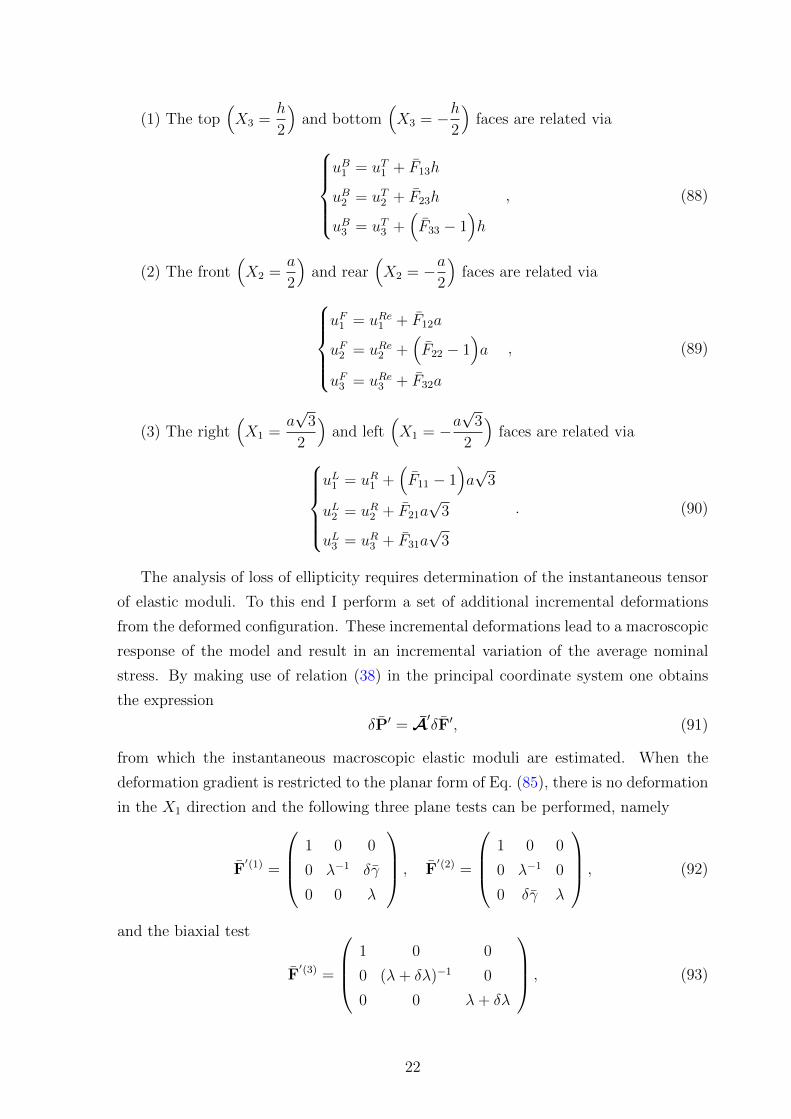
(1) The top(X3 =
h
2
)and bottom
(X3 = −h
2
)faces are related via
uB1 = uT1 + F13h
uB2 = uT2 + F23h
uB3 = uT3 +(F33 − 1
)h
, (88)
(2) The front(X2 =
a
2
)and rear
(X2 = −a
2
)faces are related via
uF1 = uRe1 + F12a
uF2 = uRe2 +(F22 − 1
)a
uF3 = uRe3 + F32a
, (89)
(3) The right(X1 =
a√
3
2
)and left
(X1 = −a
√3
2
)faces are related via
uL1 = uR1 +
(F11 − 1
)a√
3
uL2 = uR2 + F21a√
3
uL3 = uR3 + F31a√
3
. (90)
The analysis of loss of ellipticity requires determination of the instantaneous tensor
of elastic moduli. To this end I perform a set of additional incremental deformations
from the deformed configuration. These incremental deformations lead to a macroscopic
response of the model and result in an incremental variation of the average nominal
stress. By making use of relation (38) in the principal coordinate system one obtains
the expression
δP′ = A′δF′, (91)
from which the instantaneous macroscopic elastic moduli are estimated. When the
deformation gradient is restricted to the planar form of Eq. (85), there is no deformation
in the X1 direction and the following three plane tests can be performed, namely
F′(1) =
1 0 0
0 λ−1 δγ
0 0 λ
, F′(2) =
1 0 0
0 λ−1 0
0 δγ λ
, (92)
and the biaxial test
F′(3) =
1 0 0
0 (λ+ δλ)−1 0
0 0 λ+ δλ
, (93)
22

where δγ and δλ are small increments. The deformation gradient and the nominal stress
tensor increments in the principal coordinate system are
δF′(i) = F′(i) − F′ and δP′(i) = P′(i) − P′, (94)
respectively.
Note that it is impossible to fully characterize the elastic properties of transversely
isotropic materials on the basis of plane tests alone (e.g., Ogden (2008)). This means
that some of the terms of the tensor of macroscopic elastic moduli cannot be determined.
Nonetheless, the condition for the loss of ellipticity can be extracted from appropriate
combinations of the terms of the elastic tensor obtained from the planar tests. Specifi-
cally, the strong ellipticity condition (49), rewritten in the principal coordinate system
of the left Cauchy-Green strain tensor, together with the incompressibility constraint
(44) is((A′0 3333 − A′0 3322) + (A′0 2222 − A′0 3322)− 2A′0 2332
)n2
3n22 + A′0 3232n
43+
A′0 2323n42 + 2
((A′0 2232 − A′0 3332)n3
3n2 + (A′0 3323 − A′0 2223)n32n3
)> 0.
(95)
Though the individual terms A′0 3333, A′0 3322 and A′0 2222 cannot be determined, the com-
binations(A′0 3333 − A′0 3322
)and
(A′0 2222 − A′0 3322
)can be extracted from the biaxial
plane test (93) by making use of Eq. (91), Eq. (46) and the incremental incompressibil-
ity condition
δF : F−T = 0. (96)
Thus,
δF ′22 = −δF ′33
F ′22
F ′33
= −δF′33
F′233
. (97)
Applying the biaxial test deformation F′(3), and using relation (46) together with
Eq. (97), I end up with
A′0 3333 − A′0 3322 = F ′33F′33A′3333 − F ′33F
′22A′3322 =
= F ′33F′33
(A′3333 − A′3322
F ′22
F ′33
)= F ′33F
′33
δP′(3)33
δF′(3)33
,(98)
and
A′0 2222 − A′0 3322 = F ′22F′22A′2222 − F ′33F
′22A′3322 =
= F ′22F′22
(A′2222 − A′3322
F ′33
F ′22
)= F ′22F
′22
δP′(3)22
δF′(3)22
.(99)
The rest of the terms, namely, A′0 3323, A′0 2223, A′0 2232, A′0 3332, A′0 3232 and A′0 2323 are
obtained directly from the shear tests (92) by using Eq. (91) and Eq. (46).
23

The simulations were carried out by application of the commercial FE code COM-
SOL. The deformation is defined in the principal coordinate system in terms of F′, and I
make use of Eq. (85) to impose the boundary conditions (88)-(90) on the unit cell in the
material coordinate system where the FE simulation is executed. Next, the resulting
output, in terms of the mean nominal stress tensor, is transformed back to the principal
coordinate system via the relation
P′ = RPRT . (100)
An identical procedure was used to simulate the 2-D models for the laminated compos-
ites.
Compressible SEDFs were defined directly in COMSOL code. The neo-Hookean
strain energy-density functions of the phases are
Ψ(r)H =
µ(r)
2(J1 − 3) + κ(r) (J − 1)2 , (101)
where J1 = J−2/3I1 and κ is a bulk modulus. The Gent strain energy-density functions
are
Ψ(r)G = −µ
(r)
2J (r)m ln
(1− I1 − 3
J(r)m
)− µ(r) ln J (r) +
(κ(r) − 2µ(r)/3
2− µ(r)
J(r)m
)(J (r) − 1
)2.
(102)
Incompressibility was approximated by choosing bulk modulus κ(r) in each phase that is
two orders of magnitude larger than the corresponding shear modulus µ(r). A component
of the average nominal stress on a given face of the unit cell is calculated by summing
the corresponding components of the internal forces acting on the nodes of that face
and dividing the resultant force by the area of the face in the undeformed configuration.
2.4 Applications
I make use of the results of the previous sections to determine numerical and analytical
estimates for the loss of stability of fiber composites with neo-Hookean and Gent phases.
First, I examine the case when both phases are neo-Hookean. When the composite is
compressed along the fibers (i.e., Θ = 0 in Eq. (86)) the analytical expression for
the critical stretch ratio is given in Eq. (80). The corresponding predictions obtained
for composites with two different contrasts between the shear moduli of the phases are
shown in Fig. 7 as functions of the fiber volume fraction. The solid curves correspond
to k = 100 and 10.
24

0 . 0 0 . 2 0 . 4 0 . 6 0 . 8 1 . 00 . 4
0 . 5
0 . 6
0 . 7
0 . 8
0 . 9
1 . 0k = 1 0 0
k = 1 0
c ( f )
�
Fig. 7. The dependence of the critical stretch ratio on the fiber volume fraction. The solid curvescorrespond to fiber composites and the dashed curves to laminated composites. The results of thenumerical simulations are marked by triangles for k = 100 and squares for k = 10.
The corresponding expression for laminated composites that was obtained by Tri-
antafyllidis and Maker (1985) is
λc =
(1− µ
µ
)1/4
, (103)
where
µ =
(c(m)
µ(m)+c(f)
µ(f)
)−1
, (104)
and in this case µ(f) and µ(m) are shear moduli of the stiffer and the softer layers,
respectively. For comparison, the predictions of this solution are presented in Fig. 7
by the dashed curves for k = 100 and 10. The corresponding results of the numerical
simulations are marked by triangles for k = 100 and squares for k = 10. In all cases
the numerical results are in excellent agreement with the analytical ones for both the
laminated and the fiber composites.
Note that under these loading conditions φ = π/2 (i.e., m = L), meaning that
at the onset of the instability the weak surface is perpendicular to the fibers and the
deformation occurs along this surface. As was mentioned in Agoras et al. (2009b), in
agreement with experimental findings this instability is associated with vanishing shear
response in the plane transverse to the fibers. This observation is also in agreement
with the earlier findings of Qiu and Pence (1997) and Merodio and Ogden (2002).
In comparison with composites with intermediate volume fraction of fibers, the onset
of ellipticity loss occurs much later in composites with low and high fiber volume frac-
tions. As expected, the composites become more sensitive to compression as the ratio
25

0 . 0 0 . 2 0 . 4 0 . 6 0 . 8 1 . 00 . 0 0
0 . 0 5
0 . 1 0
0 . 1 5
0 . 2 0
0 . 2 5
�
���
Fig. 8. The dependence of the critical stretch ratio on the loading direction. The solid, dashed andshort-dash curves correspond to composites with fiber to matrix shear moduli ratio k = 50, 30 and 10,respectively. The simulation results are marked by squares, triangles and circles for k = 50, 30 and 10,respectively. The thin continuous curve shows the maximal loading angle Θm at which instability mayoccur. For all curves c(f) = 0.5.
between the shear moduli increases. A comparison between the results for the laminated
and the fiber composites reveals that the stable domain for the fiber composites is larger
than the one for the laminated composite, though the trends of the curves are similar.
In contrast with the results for the laminated composites, the results for the fiber com-
posite are not symmetric with respect to c(f) = 0.5. Thus, at low fiber volume fraction,
the composite is more sensitive to compression than at high fiber volume fraction.
A few representative results for the critical stretch ratio under non-aligned compres-
sion are shown in Fig. 8. The corresponding expression for λc was determined by Agoras
et al. (2009b) for the TIH model introduced in deBotton et al. (2006) in terms of the
quartic polynomial equation
λ4c cos2 Θ− λ2
c
(1− µ
µ
)2/3
+ sin2 Θ = 0. (105)
The solid, dashed and short-dashed curves correspond to fiber-to-matrix shear moduli
ratios k = 50, 30 and 10, respectively. In all cases the volume fraction of the fiber
is c(f) = 0.5. The results of the corresponding numerical simulations are marked by
squares, triangles and circles for k = 50, 30 and 10, respectively. The curves are
symmetric with respect to the loading direction Θ = 0, that is λc(Θ) = λc(−Θ), and
are also π-periodic, that is, λc(Θ) = λc(Θ +πj), j = 1, 2, 3... . Additionally I note that
λc(Θ) = 1/λc(Θ + π/2).
Comparing the analytical solution to the numerical simulations, one can observe a
26

1 0 0 2 0 0 3 0 00 . 0 0
0 . 0 5
0 . 1 0
0 . 1 5
0 . 2 0
0 . 2 5
k
���
Fig. 9. The dependence of the maximal loading direction angle on the ratio between the shear
moduli. The solid, dashed and short-dash curves correspond to volume fractions of the fiber c(f) = 0.1,0.25 and 0.5, respectively.
better agreement for higher shear moduli ratios k. However, for all cases the characte-
ristic behavior is similar and the analytical solution is the more conservative estimation
for the onset of failure. The reason for the difference is related to the fact that the an-
alytical solution is obtained for incompressible composites while in the FE simulations
the phases are slightly compressible. I emphasize that a decrease in the compressibility
of the phases, in terms of an increase in the bulk to shear moduli ratio, resulted in an
earlier onset of ellipticity loss and hence to a better agreement between the two esti-
mates. This influence of incompressibility on the onset of failure is in agreement with the
observation of Triantafyllidis et al. (2006). Additionally, I recall that the microstructure
used in the numerical simulation, while providing a fair estimate for composites with
randomly distributed fibers, is not an actual TI material.
In consistent with expectations, the value of λc approaches unity asymptotically as
k → ∞. Note that as the angle between the loading and the fiber directions increases
there exist an angle (Θm) beyond which no macroscopic instability occurs. The critical
stretch ratio corresponding to this angle is
λm =1√
2 cos Θm
(1− µ
µ
)1/3
, (106)
and it is represented in Fig. 8 by the thin continuous curve. Obviously, Θm depends on
the fiber volume fraction and shear moduli ratio, and from Eq. (105) it is easy to see
that
Θm =1
2arcsin
(1− µ
µ
)2/3
. (107)
27

0 1 0 2 0 3 0 4 0 5 00 . 2
0 . 4
0 . 6
0 . 8
1 . 0
k
�
Fig. 10. The critical stretch ratio as a function of the contrast between the phases shear moduli fordifferent loading directions. The continuous, dash and short-dashed curves correspond to Θ = 0, π/16and π/8, respectively. The results of the numerical simulation are marked by squares, triangles andcircles for Θ = 0, π/16 and π/8, respectively.
The dependence of the maximal angle Θm on the ratio between the shear moduli is
shown in Fig. 9 for fiber volume fractions c(f) = 0.5, 0.25 and 0.1 by solid, dashed, and
short-dashed curves, respectively. The domain above the curve is the one for which no
instability was detected, while in the region beneath the curve critical stretch ratios
corresponding to ellipticity loss were found. Obviously, when the shear moduli contrast
k becomes large the load direction Θm tends to π/4, corresponding to a switch of the
load along the fibers from compression to tension. Combining Eq. (106) and Eq. (107)
I end up with the expression
Θm = arctanλ2m. (108)
The physical reasoning for this value becomes clear when the rotation of the fibers under
non-aligned load is followed (e.g., deBotton and Shmuel (2009)). Thus, in the deformed
configuration the angle between the fiber and the loading directions is
θ = arctan(λ−2 tan Θ
). (109)
Eq. (108) and Eq. (109) lead to θm = π/4. At this angle the loading on the fibers
switches from compression to tension. Consequently, beyond this point no instability
is detected. Thus, one can find that the maximal loading angle Θm corresponds to the
state at which in the current configuration θ(λc) = π/4.
The dependence of the critical stretch on the contrast between the fiber to the matrix
shear moduli is presented in Fig. 10 for different loading directions. The solid, dashed
28

and short-dashed curves correspond to the analytical solution for Θ = 0, π/16 and π/8,
respectively. The numerical simulation results are presented by squares, triangles and
circles for Θ = 0, π/16 and π/8, respectively.
The numerical simulation results are in good agreement with the analytical solution
for low values of the loading angles. However, for relatively high values of this angle
the deformation needed for the onset of ellipticity loss increases and hence the effect
of the phases compressibility becomes significant. This, in turn, results in an increase
in the difference between the analytical and the numerical predictions. This is on top
of the difference stemming from the different microstructures associated with the two
estimations.
Next, I examine the responses of composites whose phases behaviors are described
by the Gent model Eq. (30). As was mentioned before, the variational estimate applied
to this model results in a close-form solution of Eq. (62) in terms of a cubic polynomial.
With this solution, the tensor of elastic moduli A given by Eq. (65) is evaluated at each
step of the loading path which is described by the loading parameters λ and Θ. When
the left-hand side of Eq. (49) becomes non-positive, instability may occur.
Remarkably, I find that for a wide range of materials and loading parameters (λ, Θ,
k, µ(m), c(f), r, J(m)m ) the value of ω(G), the solution of the optimization problem (58), is
very close to ω(H) which is the corresponding solution for the neo-Hookean composite
given in Eq. (75). Upon substitution of this expression in Eq. (58) I end up with the
following upper estimate (UE) for Ψ(TI), namely,
Ψ(UE) = −1
2
∑r=m, f
c(r)µ(r)J (r)m ln
(1− I
(r)1 (ω(H))− 3
J(r)m
). (110)
Moreover, one finds that for a large range of materials and loading parameters the
derivatives of ω(G) with respect to F are negligible and hence not only the stresses can
be analytically derived from Eq. (110), but also the tensor of elastic moduli can be easily
derived. Thus, I have that
A(UE)=∑r=m, f
(∂2Ψ(UE)
∂I(r)1 ∂I
(r)1
∂I(r)1
∂F(F)
∂I(r)1
∂F(F) +
∂Ψ(UE)
∂I(r)1
∂2I(r)1
∂F∂F(F)
). (111)
Application of the strong ellipticity condition (49) and Eq. (46) with Eq. (111) results
in closed-form estimates for the onset of macroscopic instabilities in Gent composites.
In particular, when the fiber and the matrix lock-up stretches are identical (i.e., r = 1),
for the case of compression along the fibers the critical stretch ratio can be estimated
29

from the solution of the polynomial equation((λ3
c − 1)(c(f)µ(f)α(m) + c(m)µ(m)α(f)) + µα(f)α(m))
(1− 2λc + λ2c)+(
µ(λ3c − 1) + µ
)(λ4c + 2λc − λ2
c(Jm + 3))
= 0.(112)
Note that as Jm →∞ this equation is reduced to the corresponding expression for the
neo-Hookean composite as given in Eq. (80).
To estimate the applicability range of Eq. (111), the appropriate domain in the seven
dimensional space of λ, Θ, k, µ(m), c(f), r, J(m)m should be identified. In this domain, the
derivatives of ω(G) with respect to F should be negligible and ω(G) can be approximated
by ω(H). In a way of an example, I examine the dependence of ω(G) and∂ω(G)
∂λon λ.
This is demonstrated in Fig. 11 for composites with fiber volume fraction c(f) = 0.5,
shear moduli ratio k = 100, µ(m) = 106 Pa, r = 1 and loading direction Θ = 0. The
continuous curves correspond to ω(λ) for Jm = 0.1, 1, 10, 100 and the dashed curves
to the corresponding derivatives. The thin short-dash line corresponds to ω(H) (which
is independent of λ). One can observe two regions of the functions ω(G) and∂ω(G)
∂λ, a
“fast” region and a “slow” one. The value of λs that separates these two regions is given
by the solution of the equation
ω(G)(λs)−∂ω(G)
∂λ(λs) = 0. (113)
In Fig. 11, the curve crossings that represent the solution of Eq. (113) are marked by
squares. One can observe that as long as λ > λs, that is in the “slow” region of the two
functions, ω(G) is almost identical to ω(H). In the scale of this plot the critical stretch
ratios for the four composites examined are very close and hence are marked by a single
triangle mark. Since λc > λs, in these composites the ellipticity loss occurs before the
λs is achieved. Even in the case when λc < λs the upper estimate is still usable, but the
difference in the predicted solution becomes large.
The results obtained by application of the upper estimate (112) for the critical
stretch ratio are shown in Fig. 12 for the case of aligned compression (Θ = 0). The
solid curve corresponds to shear moduli ratio k = 100, and the dashed curve to k = 50.
I emphasize that for the results shown in Fig. 12, the curves determined via the full
solution of the variational estimate (that is with ω(G) and its derivatives) lay on top of
those determined via the upper estimate of Eq. (112). The dotted curve describes the
solution of the lock-up equation due to loading in the form of Eq. (84)
λlock =1
2
(√Jm + 4−
√Jm
). (114)
The thin dashed lines are the corresponding estimates for the neo-Hookean composites.
The results of the numerical simulations are also shown in Fig. 12. The square and
30

0 . 1 0 . 2 0 . 4 0 . 6 0 . 8 1 . 00 . 0
0 . 5
1 . 0
1 . 5
2 . 0
2 . 5
0 . 0
0 . 5
1 . 0
1 . 5
2 . 0
2 . 5
�'
J m = 0 . 1J m = 1J m = 1 0J m = 1 0 0
�( H )
�
�
Fig. 11. The dependence of ω(G) and (ω(G))′ on the stretch ratio λ for the Gent composite with Θ = 0,
c(f) = 0.5, k = 100 and r = 1. The continuous curves correspond to ω(G)(λ) for Jm = 0.1, 1, 10, 100from right to left, while the dashed curves to (ω(G))′(λ). The thin short-dash line corresponds to ω(H)
for the neo-Hookean composite. The curve crossings are marked by squares. The triangle indicates thecritical stretch ratio for these composites.
circle marks correspond to simulations with k = 100 and 50, respectively. The numeri-
cal results are in good agreement with the analytical ones even in the region where the
locking effect becomes significant. In a manner similar to one mentioned in connection
with the neo-Hookean composites, the differences between the analytical and the nume-
rical results are due to the effect of compressibility in the simulations and the different
microstructures.
Note that in the region where the locking effect becomes significant, both phases
markedly stiffen and hence the contrast between their stiffnesses decreases. Conse-
quently, for small enough locking parameter of the Gent phases no instabilities are
detected. Specifically, as can be deduced for the two families of Gent composites shown
in Fig. 12, composites with k = 100 and Jm < 0.018 are stable, as well as composites
with k = 50 and Jm < 0.067. I denote the minimal value of the locking parameter
beneath which the composite is stable J(c)m . This value depends on the phase properties
but particularly on k. The critical stretch ratios corresponding to J(c)m are represented
in Fig. 12 by a thin continuous curve.
In case when the matrix is characterized by a locking parameter smaller than that of
the fiber phase (e.g., r < 1), the matrix stiffens faster than the fiber and the contrast
between the phases decreases with the deformation. In this case the composite becomes
more stable in a manner similar to the case tr = 1. The situation changes when the
fiber phase stiffens faster than the matrix phase (e.g., r > 1). In this case, the contrast
31

0 . 0 0 . 1 0 . 2 0 . 3 0 . 40 . 8 0
0 . 8 5
0 . 9 0
0 . 9 5
1 . 0 0
�
J m
Fig. 12. The dependence of the critical stretch ratio λc on the locking parameter Jm. The solidline corresponds to shear moduli ratio k = 100, and the dashed curve to k = 50. The dotted curverepresents the lock-up stretch ratio. The numerical simulation results are marked by squares and circlesfor k = 100 and 50, respectively.
between the phase responses increases with the deformation, and the composite becomes
more sensitive to compression. This finding is consistent with corresponding findings of
Agoras et al. (2009b) that were determined via the LC variational method.
Finally, the influence of the loading direction is demonstrated for composites with
c(f) = 0.5 and k = 100 in Fig. 13. Shown is the dependence of the critical stretch ratio
λc on the locking parameter Jm. The solid curve corresponds to aligned compression
(Θ = 0), the dashed and short-dashed curves represent non-aligned compression with
Θ = π/16 and π/8 respectively. The results of the numerical simulations are marked by
squares, triangles and circles for Θ = 0, π/16 and π/8, respectively. The corresponding
solutions for the neo-Hookean composites are marked by thin dashed curves. The dotted
curve describes the lock-up stretch ratios according to Eq. (114).
The difference between the numerical simulations and the analytical predictions is
due to the compressibility and microstructure differences. In a manner similar to the
one observed for the neo-Hookean composites, an increase of the loading angle requires
a decrease of the stretch ratio to achieve the onset of a failure. Additionally, for a given
locking parameter Jm there exists a loading angle Θ(c) beyond which the composite
becomes stable. The curve corresponding to this loading angle, which terminates at J(c)m
when Θ = 0, is presented in Fig. 13 by the thin continuous curve.
I conclude this section noting that in both cases of aligned loading (Fig. 12) and
32

0 . 0 0 . 1 0 . 2 0 . 3 0 . 40 . 8 0
0 . 8 4
0 . 8 8
0 . 9 2
0 . 9 6
1 . 0 0
�
J m
Fig. 13. The dependence of the critical stretch ratio λc on the locking parameter Jm for k = 100.The solid, dashed and short-dashed curves correspond to Θ = 0, π/16 and π/8, respectively. Theresults of the numerical simulations are marked by squares, triangles and circles for Θ = 0, π/16 andπ/8, respectively. The corresponding solutions for the neo-Hookean composites are marked by dashedthin lines. The locking curve is the dotted one. The thin continuous curve represents the maximalloading angle for which instabilities were detected.
non-aligned loading (Fig. 13), the onset of failures in the Gent composites can be con-
servatively estimated by the corresponding predictions for the neo-Hookean composites
even for relatively small values of Jm. The proximity between the estimates for the criti-
cal stretches is in agreement with corresponding results computed by Bertoldi and Boyce
(2008) and Agoras et al. (2009b). Bertoldi and Boyce (2008) noted that for Jm > 1 the
numerical estimates for both microscopic and macroscopic critical stretch ratios at the
onset of ellipticity loss in porous composites with Gent and neo-Hookean matrices are
almost identical when their microstructures are identical. Based on estimates computed
for specific composites with neo-Hookean and Gent phases, Agoras et al. (2009b) infer
that macroscopic instabilities may develop in non-linear incompressible fiber composites
whenever λn reaches the critical value predicted by Eq. (80) that was derived from the
TIH model of deBotton et al. (2006). Specifically, it was proposed that the estimates
for the effective isochoric and out-of-plane shear moduli of the non-linear composite in
the reference configuration will be substituted for µ and µ in Eq. (80), respectively.
A fundamental reasoning for the proximity of the various estimates computed for
composites with identical microstructures and different behaviors of the phases was
given in deBotton and Shmuel (2010). These investigators noted that the structure of
the variational estimate (57) hints at the fact that bifurcations exhibited by the compos-
33

ite should be related to corresponding bifurcations of the associated comparison com-
posite. This is because the corrector term depends only on the properties of the phases,
and hence bifurcations cannot be associated with this term. Accordingly, whenever a
secondary solution that is associated with a lower energy state branches out from the
primary solution, a corresponding secondary solution will branch out from the primary
solution for the comparison composite as well. While the precise configurations at which
the bifurcations occur in the composite and the comparison composite do not have to be
identical, if the corrector terms are small the two states should be quite close. I further
note that the proximity of the critical stretch ratios at the onset of instability in the two
composites is not limited to the vicinity of the reference configuration (as concluded by
Agoras et al. (2009b)). In fact, with an appropriate optimization over the properties of
the comparison composite, estimates for instabilities that occur at large stretch ratios
can be deduced from instability analysis of the comparison composite. Moreover, while
estimate (58) that was used throughout this work was obtained by making use of a
comparison composite with neo-Hookean phases, the general variational estimate Eq.
(57) allows to make use of comparison composites with other types of phases. Usage
of available estimates for composites with two-terms, such as Yeoh (1993) model (e.g.,
Shmuel and deBotton (2010)) or anisotropic phases (e.g., deBotton and Shmuel (2009);
Lopez-Pamies and Idiart (2010)) will improve the resulting estimates for critical stretch
ratios away from the reference configuration.
I finally note that the proximity of the critical loading states is anticipated for the
critical stretch ratios since in Eq. (57) the macroscopic deformation gradient F appears
in the expressions for the energy-density functions of both the composite Ψ and the
comparison composite Ψ0. The same cannot be inferred for the corresponding critical
stresses at the onset of ellipticity loss in the two composites since the slopes of Ψ
and Ψ0 may differ quite a bit. This observation explains why Agoras et al. (2009b)
found that while the estimates they computed for the critical stretch ratios of the neo-
Hookean and the Gent composites are in good agreement, the same cannot be said for
the corresponding estimates computed for the critical stresses.
2.5 Conclusions
In this chapter I examined both analytically and numerically the instability phenomenon
in hyperelastic fiber composites. I focused on predictions of the onset of failure due
to loss of ellipticity of the governing equations describing the homogenized behavior
of the composites. The analytical model involved a TI composite in which aligned
stiffer fibers in a softer matrix are randomly distributed in the transverse plane. The
34

nonlinear-comparison variational method of deBotton and Shmuel (2010) was utilized
to estimate the composites effective response. In particular, I examined composites with
neo-Hookean and Gents phases. Additionally, a new upper estimate for Gent composites
was introduced. In parallel, I developed a 3-D FE model and extended techniques for
numerically determining the onset of ellipticity loss.
The analytical models resulted in closed-form estimates for the critical stretch ratio
corresponding to the onset of failure. The critical stretch ratio depends mainly on the
volume fraction of the fiber and the contrast between the moduli of the fiber and the
matrix. The higher the contrast, the less compressive strain is needed for the appearance
of instabilities. The influence of the fiber volume fraction is weak for the common range
of fiber volume fraction 0.2 < c(f) < 0.5 but becomes significant in the limits of low and
high volume fractions.
In accordance with the analytical findings, the numerical simulations yielded different
results for laminate and fiber composites. It was shown that the layered composites are
more sensitive to compression than the fiber composites. Additionally, in contrast to the
layered materials, the fiber composites are more stable in the range of high fiber volume
fractions than at low ones. For non-aligned compression it is found that above a certain
loading angle no instability occurs. I demonstrate that this loading angle corresponds
to the state when the angle between the fiber and the load in the deformed configuration
is π/4. At this angle the loading on the fibers switches from compression to tension.
In the limit of small locking parameter the Gent composites become stable. This is
due to the stiffening of both the fiber and the matrix phases resulting in a decrease of
the contrast between the instantaneous moduli. Consequently, the critical stretch ratio
decreases towards the stretch ratio at which the material locks up and practically no
instability occurs. At larger values of the locking parameter it is found that the onset of
failure of the Gent composites can be quite satisfactory predicted by the corresponding
estimate for neo-Hookean composites. This finding, which is in agreement with corre-
sponding results of Bertoldi and Boyce (2008) and Agoras et al. (2009b), is explained
in the light of the nonlinear comparison variational estimate of deBotton and Shmuel
(2010).
35

Chapter 3
Macroscopic Instabilities in Anisotropic
Soft Dielectrics
In this chapter I extend the work of Dorfmann and Ogden (2010) to the class of
anisotropic electroactive materials undergoing large deformations. I introduce a general
criterion for the onset of instability for plane problems. In a way of an example I ex-
amine the class of layered media with isotropic behavior of the layers. I chose this class
for two reasons. The first is related to the fact that expressions for the coupled elec-
tromechanical behaviors of anisotropic EAPs are not available in the literature, and since
layered materials can be manufactured the outcome will correspond to a feasible class of
anisotropic materials. For this reason I also chose a widely accepted form for the phases
behavior, one that can provide an approximation to more complicated behaviors in the
limit of small to moderate deformations. The second reason stems from the fact that
for this class of materials a rigorous explicit expression for the homogenized anisotropic
energy-density function can be determined (deBotton and Tevet-Deree, 2006; Bertoldi
and Gei, 2011). By making use of this expression for their overall energy-density func-
tion, I identify the stable domain of these materials under different loading conditions
and demonstrate the significance of their overall symmetry.
3.1 Theory
In order to determine the onset of instabilities I seek a solution for Eq. (20) in the form
vi = vif(a · x), p = qf ′(a · x), Di = dif′(a · x), (115)
where f is a continuous and sufficiently differentiable function and a is a unit vector.
Assume that the material undergoes plane-strain deformations and there is no out-
of-plane component of the electric displacement field. By making use of the incompress-
ibility constraint div v = 0 together with Maxwell equation for D, it can be found that
viai = 0 and diai = 0 and hence di = γvi, where γ is a real coefficient. Thus, upon
substitution of Eq. (115) together with the relation di = γvi in Eq. (20) and eliminating
the pressure increment, I end up with a polynomial equation for ξ ≡ a2/a1, namely
Γ6ξ6 + Γ5ξ
5 + Γ4ξ4 + Γ3ξ
3 + Γ2ξ2 + Γ1ξ + Γ0 = 0. (116)
36

The coefficients Γi are given in terms of the electroelastic moduli
Γ0 =K2122 −A2121D22,
Γ1 =2 (A2121D12 + (A1121 −A2122)D22 −K122 (K112 +K121 −K222)) ,
Γ2 =−A2121D11 − 4 (A1121 −A2122)D12 − (A1111 − 2A1122 − 2A1221 +A2222)D22
+ 2K122 (K111 −K122 −K221) + (K112 +K121 −K222)2 ,
Γ3 =2((A1121 −A2122)D11 + (A1111 − 2A1122 − 2A1221 +A2222)D12
+ (A1222 −A1112)D22 + (K121K122 − (K111 −K122 −K221)(K112 +K121 −K222))),
Γ4 =− (A1111 − 2A1122 − 2A1221 +A2222)D11 + 4 (A1112 −A1222)D12
−A1212D22 + (K122 +K221 −K111)2 − 2K121 (K112 +K121 −K222) ,
Γ5 =2 ((A1222 −A1112)D11 +A1212D12 +K121(K111 −K122 −K221)) ,
Γ6 =K2121 −A1212D11.
(117)
Whenever a real solution for Eq. (116) exists, instabilities may occur. The correspond-
ing value of γ that relates the amplitudes of the incremental changes in the electric
displacement and the displacement is
γ =K121ξ
3 + (K111 −K122 −K221) ξ2 + (K222 −K112 −K121) ξ +K122
D22 + (D11ξ − 2D12) ξ. (118)
I conclude this section noting that condition (116) is an extension to the class of
anisotropic materials of the corresponding result derived by Dorfmann and Ogden (2010)
for the class of isotropic materials. In the following section I apply this general crite-
rion to a specific class of anisotropic materials for which analytical expressions for the
electroelastic moduli can be determined. Yet, before I proceed to this task, I stress
that condition (116) can be used in conjunction with numerical simulations of more
general anisotropic materials for which analytical solutions cannot be determined. In
these cases estimates for the electroelastic moduli can be determined with appropriate
simulations of small variations in the boundary conditions.
3.2 Applications to Soft Dielectric Laminates.
In a way of an example I examine the class of layered composites with two isotropic and
incompressible phases. As was mentioned in the introduction, from a practical viewpoint
this is a feasible class of materials and from a theoretical viewpoint their overall behavior
can be determined explicitly (deBotton et al. (2007); Tevet-Deree (2008)). The resulting
closed form expressions for the electroelastic moduli can be conveniently utilized in the
37

stability analysis. Bertoldi and Gei (2011) considered this class of composites under
specific loading conditions that are aligned with the layers. Here, I extend this analysis
and examine the influence of more general loadings on the onset of instabilities. In
this regard it is worth mentioning that enhancement of the mechanical response to
electrical excitation crucially depends on the ability to furnish appropriate soft modes
of deformation by controlling the angle between the layers and the electrical excitation
field deBotton et al. (2007); Tevet-Deree (2008).
The volume fractions of the phases are c(m) and c(f) = 1 − c(m). Geometrically,
the layers are characterized by their thicknesses h(m) = c(m)h and h(f) = c(f)h, where
h = h(m) + h(f). Here and thereafter I denote a field in phase r by (•)(r), in particular
(•)(f) and (•)(m) correspond to the stiffer and the softer phases, respectively. The
direction normal to the layers plane in the undeformed configuration is the laminate
direction N, and M is a unit vector tangent to the interface (see Fig. 20). Specifically,
in terms of the referential lamination angle Θ,
N = sin Θ e1 + cos Θ e2 and M = cos Θ e1 − sin Θ e2. (119)
Assuming that all fields are homogeneous in each phase, I have that the mean deforma-
tion gradient, the nominal electric field and the electric displacement are
F = c(m)F(m) + c(f)F(f), E0 = c(m)E0 (m) + c(f)E0 (f), D0 = c(m)D0 (m) + c(f)D0 (f).
(120)
Following deBotton (2005), by making use of the displacement continuity condition
across the interface
F(m) = F(I + c(f)αM⊗ N
), F(f) = F
(I− c(m)αM⊗ N
), (121)
where the scalar α is obtained from the traction continuity condition(P(m) −P(f)
)· N = 0. (122)
Similarly, since the interfaces are charge free, the continuity condition for the electric
displacement is (D0 (m) −D0 (f)
)· N = 0 or D0 (m) −D0 (f) = βM, (123)
and, together with the last of Eq. (120), I conclude that
D0 (m) = D0 + c(f)βM and D0 (f) = D0 − c(m)βM, (124)
where β is a scalar to be determined from the continuity condition for the nominal
electric field (E0 (m) − E0 (f)
)· M = 0. (125)
38

The energy-density function of the isotropic phases can be expressed in terms of
the invariants of the Cauchy-Green strain tensor C ≡ FTF and the referential electric
displacement D0 Dorfmann and Ogden (2005). A set of six invariants can be expressed
in the form
I1 = TrC, I2 =1
2(I2
1 − Tr(CC)), I3 = det C,
I4e = D0 ·D0, I5e = D0 ·CD0, I6e = D0 ·C2D0.(126)
Thus, the energy-density functions of the isotropic phases can be written as scalar
functions of these six invariants in terms of the local fields F(r) and D0 (r). In particular,
for composites with neo-Hookean dielectric phases the energy-density functions are
Φ(r)(F(r),D0 (r)) =µ(r)
2
(I
(r)1 − 3
)+
1
2ε(r)I
(r)5e , (127)
where µ(r) are the shear moduli and ε(r) are the dielectric constants of the two phases.
In this work I restrict the attention to this class of phase behaviors for two reasons.
The first stems from the fact that explicit expressions for the corresponding effective
electroelastic moduli can be determined. The second is that, at moderate stretch levels
where instabilities frequently onset, this energy-density function can be viewed as a first
order estimate for more general energy-density functions (e.g., Shmuel and deBotton,
2010). Moreover, in the purely mechanical case it was recently found that the critical
stretch ratios at which instabilities occur in composites with neo-Hookean phases can
serve as good estimates for corresponding critical stretch ratios for composites with Gent
phases (Bertoldi and Boyce, 2008; Agoras et al., 2009b; Rudykh and deBotton, 2012).
Upon substitution of Eq. (127), with the aid of Eqs. (22) for P(r) and E0(r), in
Eqs. (122) and (125) it can be found that
α =µ(f) − µ(m)
c(m)µ(f) + c(f)µ(m)
FN · FM
FM · FM, (128)
and
β =µ(m)ε(m) − µ(f)ε(f)
(c(m)µ(f) + c(f)µ(m)) ε
FD0 · FM
FM · FM+
µ(f) − µ(m)
c(m)µ(f) + c(f)µ(m)D0 · M, (129)
where ε = c(m)ε(m) + c(f)ε(f).
Once the solution for the boundary value problem is given in terms of the local
fields in both phases, the expression for the macroscopic energy-density function of the
composite can be expressed as the weighted sum of the energy-density functions of the
two phases, namely
Φ(F, D0) =∑r=m,f
c(r)Φ(r)(F, D0). (130)
39

0D
λ
N
M
2x
1x
Fig. 14. Electroactive layered composite subjected to electric excitation
The expressions for the average nominal stress and electric field are
P =1
2
∑r=m,f
c(r)
(µ(r)∂I
(r)1
∂F+
1
ε(r)∂I
(r)5
∂F
)− pF−T , (131)
and
E0 =1
2
∑r=m,f
c(r)
ε(r)∂I
(r)5
∂D0. (132)
The corresponding overall electroelastic moduli are
A0ijkl =
1
2
∑r=m,f
c(r)
(µ(r) ∂
2I(r)1
∂F∂F+
1
ε(r)∂2I
(r)5
∂F∂F
),
G0ijk =
1
2
∑r=m,f
c(r)
ε(r)∂2I
(r)5
∂F∂D0,
E0ij =
1
2
∑r=m,f
c(r)
ε(r)∂2I
(r)5
∂D0∂D0.
(133)
Finally, with the aid of Eqs. (117) the appropriate coefficients can be determined and
substituted in the general instability condition (116).
I examine the behavior of a composite which is subjected to electric excitation cor-
responding to a nominal electric displacement in the form
D0 = D0 (cosφe1 + sinφe2) , (134)
and macroscopically stretched according to the homogeneous deformation gradient
F = λe1 ⊗ e1 + λ−1e2 ⊗ e2 + e3 ⊗ e3. (135)
Consider first the case when φ = π/2 and the angle of lamination relative to the applied
loading varies. The loading configuration is schematically shown in Fig. 20. I make use
of Eqs. (116) and (133) to determine the stable domain of the layered EAP.
40

0 1 2 3 4 5 60 . 20 . 40 . 60 . 81 . 01 . 21 . 41 . 6
����
�����
����
������
D n
( a )
0 2 4 6 8 1 00 . 40 . 60 . 81 . 01 . 21 . 41 . 61 . 82 . 0
( b )
��
������ ���
��
D n
0 2 4 6 8 1 0 1 20 . 20 . 40 . 60 . 81 . 01 . 21 . 41 . 6
����
�����
����
������
D n
( c )
0 2 4 6 8 1 0 1 2 1 4 1 60 . 40 . 60 . 81 . 01 . 21 . 41 . 61 . 82 . 0
( d )
��
������ ���
��
D n
Fig. 15. Bifurcation diagrams of layered materials with different lamination angles as functions ofthe critical stretch ratio and electric displacement field. The volume fractions of the stiffer phase isc(f) = 0.2 for (a) and (b) and c(f) = 0.8 for (c) and (d); the phase constant ratios are k = t = 10.Figures (a) and (c) are for small lamination angles, and figures (b) and (d) are for large laminationangles.
Shown in Fig. 15 are the analytical estimates for the onset of instabilities in materials
with c(f) = 0.2 (Figs. 15a and 15b) and c(f) = 0.8 (Figs. 15c and 15d), stiffer to softer
shear moduli ratio k ≡ µ(f)/µ(m) = 10 and dielectric constants ratio t ≡ ε(f)/ε(m) =
10. Following Triantafyllidis et al. (2006), I plot failure surfaces that separate stable
domains from those in which instabilities may develop. These bifurcation diagrams
are presented as functions of the critical stretch ratio λc and the critical electrostatic
excitation Dn = D0/√µ(m)ε(m) for composites with different lamination angles.
Note that in agreement with earlier findings (e.g., Triantafyllidis and Maker, 1985;
Nestorovic and Triantafyllidis, 2004; Agoras et al., 2009b; Rudykh and deBotton, 2012),
in the purely mechanical case (Dn = 0) the composites become unstable only under
compression in the lamination direction. Moreover, as the angle between the loading and
the lamination directions increases there exists an angle beyond which no macroscopic
41
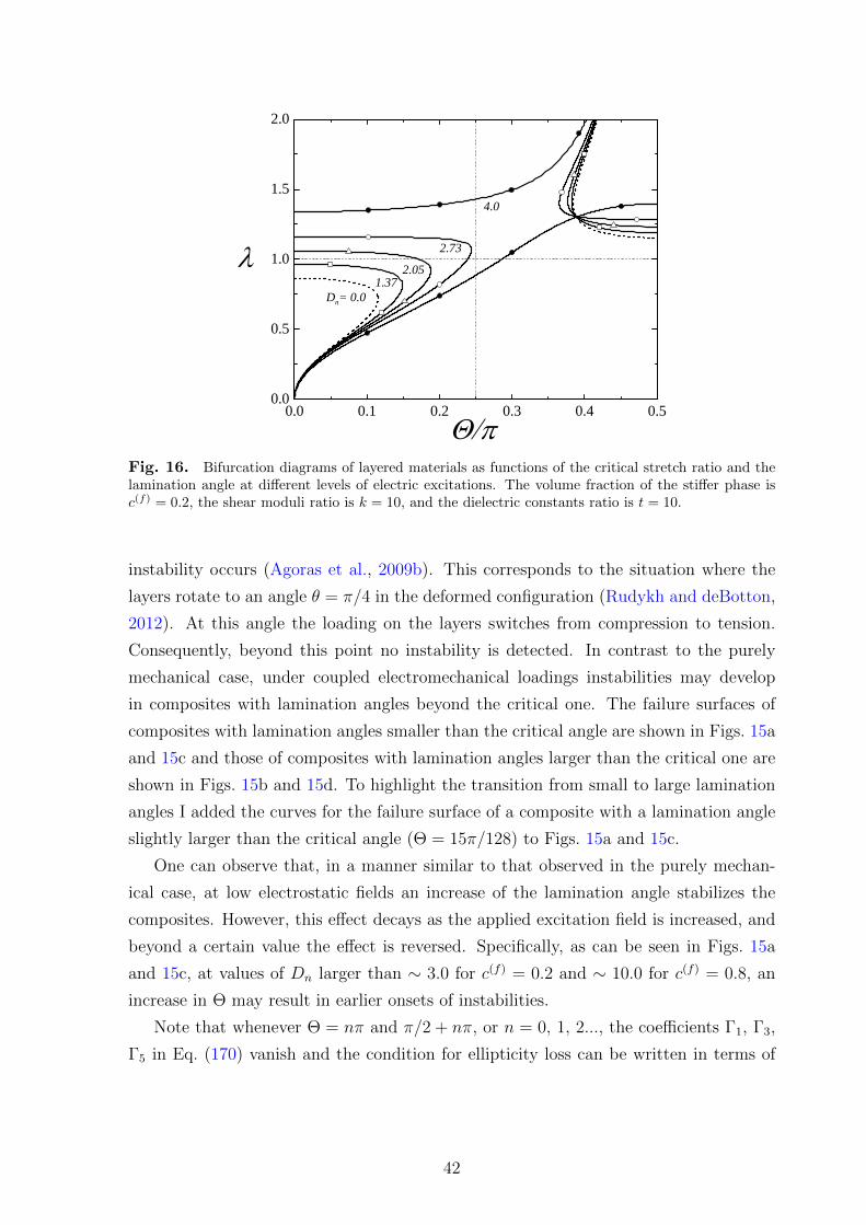
0 . 0 0 . 1 0 . 2 0 . 3 0 . 4 0 . 50 . 0
0 . 5
1 . 0
1 . 5
2 . 0
4 . 0
���
2 . 7 3
1 . 3 7 2 . 0 5D n = 0 . 0
�
Fig. 16. Bifurcation diagrams of layered materials as functions of the critical stretch ratio and thelamination angle at different levels of electric excitations. The volume fraction of the stiffer phase isc(f) = 0.2, the shear moduli ratio is k = 10, and the dielectric constants ratio is t = 10.
instability occurs (Agoras et al., 2009b). This corresponds to the situation where the
layers rotate to an angle θ = π/4 in the deformed configuration (Rudykh and deBotton,
2012). At this angle the loading on the layers switches from compression to tension.
Consequently, beyond this point no instability is detected. In contrast to the purely
mechanical case, under coupled electromechanical loadings instabilities may develop
in composites with lamination angles beyond the critical one. The failure surfaces of
composites with lamination angles smaller than the critical angle are shown in Figs. 15a
and 15c and those of composites with lamination angles larger than the critical one are
shown in Figs. 15b and 15d. To highlight the transition from small to large lamination
angles I added the curves for the failure surface of a composite with a lamination angle
slightly larger than the critical angle (Θ = 15π/128) to Figs. 15a and 15c.
One can observe that, in a manner similar to that observed in the purely mechan-
ical case, at low electrostatic fields an increase of the lamination angle stabilizes the
composites. However, this effect decays as the applied excitation field is increased, and
beyond a certain value the effect is reversed. Specifically, as can be seen in Figs. 15a
and 15c, at values of Dn larger than ∼ 3.0 for c(f) = 0.2 and ∼ 10.0 for c(f) = 0.8, an
increase in Θ may result in earlier onsets of instabilities.
Note that whenever Θ = nπ and π/2 + nπ, or n = 0, 1, 2..., the coefficients Γ1, Γ3,
Γ5 in Eq. (170) vanish and the condition for ellipticity loss can be written in terms of
42

the bi-cubic polynomial
Γ6ξ6 + Γ4ξ
4 + Γ2ξ2 + Γ0 = 0. (136)
For the case Θ = 0 this result was previously determined by Bertoldi and Gei (2011).
The corresponding relation between the critical stretch ratio and the electric excitation
is
λc =
(1− µ
µ+D2
µε
(1− ε
ε
))1/4
, (137)
where
µ = c(m)µ(m) + c(f)µ(f), µ =
(c(m)
µ(m)+c(f)
µ(f)
)−1
and ε =
(c(m)
ε(m)+c(f)
ε(f)
)−1
. (138)
Here I find that for the case Θ = π/2 the critical stretch ratio is
λc =
(1− µ
µ
)−1/4(1 +
D2
µε
(1− ε
ε
))1/4
. (139)
In the purely mechanical case (Dn = 0), both expressions (137) and (139) appropriately
reduce to the well-known result of Triantafyllidis and Maker (1985).
The bifurcation diagrams of composites with phase volume fractions c(f) = 0.2 and
material constants similar to the ones considered previously are shown in Fig. 16. To
highlight the role of the anisotropy of the material this time the critical stretch ratios
are presented as functions of the lamination angle for different electrostatic loading
conditions. The curves with square, triangle, white circle and black circle marks cor-
respond to excitation fields Dn = 1.37, 2.05, 2.73 and 4.0, respectively. The dashed
curve represents the purely mechanical case. This curve is symmetric with respect to
the loading direction Θ = 0, that is λc(Θ) = λc(−Θ), and is also π-periodic, that is,
λc(Θ) = λc(Θ + πj), j = 1, 2, 3... . Additionally, I note that λc(Θ) = 1/λc(Θ + π/2).
In contrast to the purely mechanical case, in general, the electromechanical failure sur-
faces do not possess the last symmetry due to the different contributions of the electric
excitation in the two perpendicular cases.
One can observe that in the purely mechanical case composites with larger lamination
angle become more stable (Nestorovic and Triantafyllidis, 2004). This is also true at
moderate levels of electric excitations where I note that the topmost curves that emerge
from the Θ = 0 axis have a negative slope up to a certain lamination angle beyond
which no instability is detected. However, at large enough electrostatic excitation the
direction of the slope is reversed (e.g., the curve marked by black circles that corresponds
to Dn = 4.0). Furthermore, under large electrostatic fields instabilities may occur at
any lamination angle.
43

0 . 0 0 . 2 0 . 4 0 . 6 0 . 8 1 . 00 . 4
0 . 6
0 . 8
1 . 0
1 . 2
1 . 41 . 5
s t a b l e
�����
����
����
���
c ( f )
u n s t a b l e
Fig. 17. The failure surfaces of layered composites with different lamination angles as functionsof the critical stretch ratio and volume fraction of the stiffer phase subjected to a fixed electrostaticexcitation Dn = 4.0. The shear moduli ratio is k = 10, and the dielectric constants ratio is t = 10.
A somewhat different observation is associated with the case where the layers are
aligned with the electric field (i.e., Θ = π/2). In this limit the electric field stabilizes the
material and larger tensile stretch ratios (that correspond to larger compressions along
the layers) are required for the onset of instabilities. At moderate levels of electric fields,
as the lamination angle of the composite is decreased towards Θ = 0 the critical stretch
ratio increases. However, once again at large levels of electric excitations the trend is
reversed (see the curve corresponding to Dn = 4.0). In this case, as the lamination
angle is decreased from Θ = π/2 instabilities may occur at lower stretch ratios.
The influence of the volume fraction of the phases on the stability of the composites is
depicted in Fig. 17. Bifurcation diagrams for composites with lamination angles Θ = 0,
π/16, π/8 and 3π/16 subjected to electric excitation Dn = 4.0 are plotted as functions
of the volume fraction of the stiffer phase (the dashed curve and the continuous curves
marked by squares, triangles and circles, respectively).
At both limits of dilute volume fractions of the stiff and the soft phases the materials
are stable. Note, however, that the composites with low volume fractions of the stiffer
phase are less stable than those with higher concentration of the stiff phase. This
tendency is more pronounced for composites with larger lamination angles, for which at
the low concentration end the critical stretch ratio is higher than the one for composites
with Θ = 0. Conversely, when the volume fraction of the stiffer phase is higher, the
critical stretch ratio is lower than the one determined for Θ = 0 and at high enough
44

0D
λ N
M
ϕ2x
1x
Fig. 18. Electroactive layered composite subjected to electric excitation
volume fractions the material is stable under the applied electrostatic excitation. I
emphasize however that at higher electrostatic excitations this trend is reversed, and
composites with large lamination angle become less stable even with c(f) > 0.5. This can
be deduced from Fig. 15c that corresponds to materials with c(f) = 0.8. Specifically, note
the failure surface for Θ = 15π/128 (marked with clear triangles) that demonstrates that
at Dn > 10 the unstable domain of this material is larger than the ones for composites
with smaller lamination angles.
Next, consider the case when the composite is subjected to aligned deformation,
i.e., Θ = 0 in Eq. (135) and the angle of applied electric field φ in Eq. (134) varies. A
schematic representation of this loading mode is depicted in Fig. 18. In this case, the
non-zero components of the electroelastic moduli are
E11 = 1/ε, E22 = E33 = 1/ε, (140)
1
2G111 = G122 = G133 = G212 = G313 =
D0λ cosφ
ε, G121 = G211 =
D0 sinφ
λε1
2G222 = G233 = G323 =
D0 sinφ
λε,
(141)
A1111 = A3131 = A3232 = λ2
(µ+
D0 2 cos2 φ
ε
),
A1121 = A1211 = A2122 = A2221 = A3132 = A3231 =D0 2 cosφ sinφ
ε,
A1313 = A2323 = A3333 = µ, A1212 =
(µ+
D0 2 sin2 φ
ε
)λ−2,
A1221 = A2112 =D0 2
2λ2
ε− εεε
(1− cos 2φ) +µ− µλ2
A2121 = A1111 +A1221, A2222 = A3232 =
(µ+
D0 2 sin2 φ
ε
)λ−2.
(142)
Obviously, for the cases when φ = nπ and π/2 +nπ, where n = 0, 1, 2, ..., the condition
for ellipticity loss (116) reduces to the bi-cubic polynomial Eq. (136). In the case when
45

0 5 1 0 1 5 2 0 2 5 3 00 . 5 0
0 . 7 5
1 . 0 0
1 . 2 5
1 . 5 0
1 . 7 5
2 . 0 0
� ���
� ���
� ���
�� ���
��� ��
D n
�
Fig. 19. Bifurcation diagrams of layered materials subjected to aligned stretch and electrostaticexcitation at different angles as functions of the critical stretch ratio and electric displacement. Thevolume fraction of the stiff phase is c(f) = 0.8 and the contrasts between the elastic and dielectricmoduli are k = t = 10.
φ = nπ the critical stretch ratio can be explicitly determined.
λc =
(1− µ
µ
)1/4(1 +
D2
µε
(1− ε
ε
))−1/4
. (143)
Naturally, this expression is the reciprocal of the one given in Eq. (139).
Bifurcation diagrams as functions of λc and Dn are presented in Fig. 19 for c(f) = 0.8,
and contrast between the shear moduli k = 10 and dielectric constants t = 10. The
diagrams are shown for different angles φ = 0, 3π/16, 5π/16, 7π/16, 15π/32 and π/2.
These correspond to the continuous curves marked by triangles, solid squares, circles,
solid circles, squares and the dashed curve, respectively. The regions beneath the curves
correspond to the unstable domains.
The influence of the angle of the applied electric displacement shows that the most
sensitive structure is the one with φ = π/2, as its bifurcation curve lies above the ones
for φ < π/2. It is easy to see from Fig. 19 that for some values of φ the composite
becomes stable even at large intensities of electric excitation. For example, a composite
subjected to the electric excitations at φ = 3π/16 is stable even when subjected to large
compressive stretch ratios along the layers.
46

Chapter 4
Microscopic Instabilities in EAPs
Electromechanical instabilities in composite media may occur at any scale. To identify
the onset of bifurcations, the Bloch-Floquet technique is applied to periodic media.
Motivated by possible applications where the electric excitation is controlled by the
potential, here, contrary to the previous work of Bertoldi and Gei (2011) the analysis is
performed in terms of the referential electric field instead of electric displacement. To
connect the microscopic instability analysis to the macroscopic one, the corresponding
macroscopic instability criterion is derived in terms of the referential electric field.
4.1 Theory.
Consider a layered dielectric composite made out of two incompressible phases with
volume fractions c(m) and c(f) = 1−c(m). Here and thereafter, the fields and parameters
of the stiffer and the softer phases are denoted by superscripts (•)(f) and (•)(m), re-
spectively. Geometrically, the layers are characterized by their thicknesses h(m) = hc(m)
and h(f) = hc(f). The direction normal to the layer plane is the laminate direction N,
and M is a unit vector tangent to the interface, both in the undeformed configuration
(see Fig. 20). Assuming that along the primary branch of the solution all the fields are
homogeneous in each phase, I have that the mean nominal electric field in the composite
is
E0 = c(m)E0 (m) + c(f)E0 (f). (144)
The continuity condition on the electric field is(E0 (m) − E0 (f)
)· M = 0 or E0 (m) − E0 (f) = βN, (145)
where β is a scalar. Accordingly, the referential electric field in each phase can be
expressed in the form
E0 (m) = E0 + c(f)βN and E0 (f) = E0 − c(m)βN. (146)
Since the interface is charge free, the continuity condition on the referential electric
displacement field is (D0 (m) −D0 (f)
)· N = 0. (147)
47

λ
N
ME
Fig. 20. Electroactive layered composite subjected to electric excitation.
For incompressible laminates the displacement continuity condition (deBotton, 2005)
leads to
F(m) = F(I + c(f)αM⊗ N
)and F(f) = F
(I− c(m)αM⊗ N
), (148)
where α is a constant. The corresponding interface stress continuity condition (deBotton
et al., 2007; Tevet-Deree, 2008) is(P(m) −P(f)
)· N = 0. (149)
Once the constitutive relations for phases are prescribed, the constants α and β can be
determined from the continuity conditions (147) and (149). This completes the solution
up to a bifurcation point.
To determine the onset of instabilities in the composites an analysis similar to that
used by Triantafyllidis and Maker (1985) and Bertoldi and Gei (2011) is adopted. In
each phase I seek a solution of (20) in the form
vi = vi(x2) exp(ik1x1), p = q(x2) exp(ik1x1), Ei = ei(x2) exp(ik1x1), (150)
where k1 is the wave number along the x1-direction. The incompressibility constraint
together with the absence of the electric field vorticity provide two equations for vi and
ei
v′2 = −ik1v1 and e′1 = ik1e2, (151)
where the notation (•)′ = (•),2 is introduced. The resulting incremental governing
48

x1
h(m)
h(m)
h(f)
x2
m+
m-
f
Fig. 21. The unit cell of the layered media.
equations (20) reads
k21 (A1122 +A1221 −A1111) v1 + ik1 (2A1112 −A1222) v′1 +A1212v
′′1 − k2
1A1121v2 +
ik1G111e1 + ik1 (G112 + G121) e2 + G122e′2 − ik1q = 0, (152)
k21 (2A2122 −A1121) v1 + ik1 (A1221 +A1122 −A2222) v′1 +A1222v
′′1 − k2
1A2121v2 +
ik1G121e1 + ik1 (G122 + G221) e2 + G222e′2 − q′ = 0, (153)
k21 (G122 + G221 − G111) v1 + ik1 (G112 + G121 − G222) v′1 + G122v
′′1 − k2
1G121v2 +
ik1E11e1 + 2ik1E12e2 + E22e′2 = 0, (154)
Equations (151)-(154) provide a set of 6 linear homogeneous first order differential equa-
tions that depends on the vector of 6 unknowns u = (v1, v2, e1, e2, q, v′1)
Ru = u′. (155)
The components of the matrix R are given in Appendix C. The solution of the system
can be determined in the form
u = BZs, (156)
where s is an arbitrary constant vector that will be determined later from the continuity
and quasi-periodicity conditions on the unit cell. In (156), Z(x2) = diag[exp (zx2)] is
the diagonal matrix of the eigenvalues vector z of the matrix R and the corresponding
eigenvectors of R are the columns of the matrix B.
Consider the periodic unit cell (Fig. 21) of the layered composite. The quasi periodic
boundary conditions are
u (x2 + h) = u (x2) exp(ik2h), (157)
where k2 ∈ [0, 2π/h) is the solution periodicity parameter, also referred to as Floquet
49

parameter. In the interval 0 < x2 < h+ h(m) the solution (156) attains the form
u(x2) =m
Bm
Z(x2)m−s , 0 < x2 < h(m),
u(x2) =f
Bf
Z(x2)fs, h(m) < x2 < h,
u(x2) =m
Bm
Z(x2)m+s , h < x2 < h+ h(m), (158)
wheremz,
fz are the eigenvalues of R in which the electroelastic moduli correspond to the
appropriate phase,m
B andf
B are the corresponding matrices of eigenvectors. Substitution
of (158) into (157) yields
m+s = exp(ik2h)
(m
Z(h)
)−1m−s . (159)
The jump conditions of the incremental fields at the interfaces are
[[v]] = 0, [[T]]n = 0, [[D]] · n = 0 and n× [[E]] = 0, (160)
where n = F−T N is normal to the interface at the current configuration, and the
notation [[•]] ≡ (•)+ − (•)− is used. By making use of (150) and (151) the jump
conditions (160) are
[[v1]] = 0, [[v2]] = 0, [[e1]]n2 − [[e2]]n1 = 0, (161)
[[ik1(A1111 −A1122 + p)v1 +A1112v′1 + ik1A1121v2 + G111e1 + G112e2 − q]]n1+
[[ik1(A1211 −A1222)v1 +A1212v′1 + ik1(A1221 + p)v2 + G121e1 + G122e2]]n2 = 0,
(162)
[[ik1(A2111 −A2122)v1 + (A2112 + p)v′1 + ik1A2121v2 + G211e1 + G212e2]]n1+
[[ik1(A2211 −A2222 − p)v1 +A2212v′1 + ik1A2221v2 + G221e1 + G222e2 − q]]n2 = 0,
(163)
[[ik1(G111 − G221)v1 + G121v′1 + ik1G211v2 + E11e1 + E12e2]]n1+
[[ik1(G112 − G222)v1 + G122v′1 + ik1G212v2 + E12e1 + E22e2]]n2 = 0,
(164)
Equations (161)-(164) can be written in the form [[Qu]] = 0. The non-zero entries of
the matrix Q are
Q11 = Q22 = 1, Q33 = n2, Q34 = −n2,
Q41 = ik1
((A1111 −A1122 + p)n1 + (A1211 −A1222)n2
)Q42 = ik1
(A1121n1 + (A1211 + p)n2
), Q43 = G111n1 + G121n2, Q44 = G112n1 + G122n2,
Q45 = −n1, Q46 = A1112n1 +A1212n2,
Q51 = ik1
((A2111 −A2122)n1 + (A2211 −A2222 − p)n2
), Q52 = ik1(A2121n1 +A2221n2),
Q53 = G211n1 + G221n2, Q54 = G212n1 + G222n2, Q55 = −n2,
Q56 = (A2112 + p)n1 +A2212n2,
Q61 = ik1
((G111 − G221)n1 + (G112 − G222)n2
), Q62 = ik1(G211n1 + G212n2),
Q63 = E11n1 + E12n2, Q64 = E12n1 + E22n2, Q66 = G121n1 + G122n2. (165)
50

Finally, upon usage of (158) I have that
m
Qm
Bm
Z(h(m)
)m−s =
f
Qf
Bf
Z(h(m)
) fs,
m
Qm
Bm
Z(h)m+s =
f
Qf
Bf
Z(h)fs. (166)
The combination of (159) and (166) leads to the condition for the existence of a non-
trivial solution
det
[(m
Qm
B
)−1 f
Qf
Bf
Z(h(f))( f
Qf
B
)−1m
Qm
Bm
Z(h(m)
)− I exp(ik2h)
]= 0. (167)
When condition (167) is satisfied for a combination of mechanical and electrical loads,
a solution in the form of Eq. (150) that satisfies Eqs. (157) and (158) exists where k2
represents the scale of the periodicity of the solution. A similar condition was derived
by Triantafyllidis and Maker (1985) for the purely mechanical case and by Bertoldi and
Gei (2011) for layered composites with isotropic neo-Hookean phases subjected to a
pre-stretch along the layers and electrical displacement excitation perpendicular to the
surface.
In the preceding analysis no assumption regarding the phase behavior is made and
the composites with anisotropic phases can be examined. Moreover, the derived condi-
tion can be used for any planar combination of mechanical and electrical loads and is
not restricted to the aligned pre-stretch and perpendicular electric excitation (Bertoldi
and Gei, 2011).
I recall that Geymonat et al. (1993) rigorously showed in the purely mechanical
case that the macroscopic instability onset corresponds to the existence of a non-trivial
solution in the long-wave limit k1h → 0. A more compact analysis similar to that
used by Hill and Hutchinson (1975) can be used for this specific limit of long waves.
In the content of the coupled problem, Bertoldi and Gei (2011) demonstrated that
the macroscopic instability analysis agrees with the onset of long wave instabilities in
layered composites with isotropic neo-Hookean phases subjected to a pre-stretch along
the layers and electrical displacement excitation perpendicular to the layers.
Motivated by these works I seek a solution for (20) in the form
vi = vif(a · x), p = qf ′(a · x), Ei = eif′(a · x), (168)
where f is a continuous and sufficiently differentiable function, a is a unit vector; vi, ei
and q are incremental macroscopic quantities which are independent of x. The incom-
pressibility constraint together with the last of (19) provide additional equations for vi
and ei. In particular, for a plane problem
v1 = −ξv2 and e1 = ξ−1e2, (169)
51

where ξ ≡ a2/a1. Upon substitution of expressions (168) together with (169) into (20),
elimination of the pressure increment leads to a polynomial equation in ξ, namely
Γ6ξ6 + Γ5ξ
5 + Γ4ξ4 + Γ3ξ
3 + Γ2ξ2 + Γ1ξ + Γ0 = 0, (170)
where the coefficients Γi are given by the electroelastic moduli as follows
Γ0 = G2121 −A2121E11, (171)
Γ1 = 2 (−A2121E12 + (A1121 −A2122) E11 + G121 (G221 + G122 − G111)) , (172)
Γ2 = −A2121E22 + 4 (A1121 −A2122) E12 − (A1111 − 2A1122 − 2A1221 +A2222) E11
− 2G121 (G112 + G121 − G222) + (G122 + G221 − G111)2 ,(173)
Γ3 = −2((A1112 −A1222) E11 + (A1111 − 2A1122 − 2A1221 +A2222) E12
+ (A2122 −A1121) E22 + (G121G122 − (G111 − G122 − G221)(G112 + G121 − G222))),
(174)
Γ4 = − (A1111 − 2A1122 − 2A1221 +A2222) E22 − 4 (A1112 −A1222) E12
−A1212E11 + (G112 + G121 − G222)2 + 2G122 (G111 − G122 − G221) ,(175)
Γ5 = 2 ((A1222 −A1112) E22 −A1212E12 + G122(G112 + G121 − G222)) , (176)
Γ6 = G2122 −A1212E22. (177)
When a real solution of (170) exists an instability associated with plane waves may oc-
cur. Note that the general condition (170) can be utilized for the macroscopic instability
analysis of multiphase hyperelastic dielectrics since no restricting assumption was made
in its derivation. Once the macroscopic electroelastic moduli are determined either via a
homogenization technique or numerically (Rudykh and deBotton, 2012, for mechanical
loads), the stable domains can be deduced from (170) for any microstructure and any
planar mechanical and electrical loading.
In the case of laminated composites going back to Eqs. (147) and (149) from which
the solution for the boundary value problem can be deduced, the energy-density function
of the composite can be expressed as the weighted sum of the phase energy-density
functions, namely
Ψ(F, E0) =∑r=m,f
c(r)Ψ(r)(F, E0). (178)
The average nominal stress tensor and electric displacement are
P =∂Ψ
∂F− pF−T and D0 = − ∂Ψ
∂E0. (179)
52

The macroscopic electroelastic moduli are given by
A0ijkl =
∂2Ψ
∂F∂F, G0
ijk =∂2Ψ
∂F∂E0and E0
ij =∂2Ψ
∂E0∂E0. (180)
Together with (17) the electroelastic moduli (180) provide the coefficients for the poly-
nomial equation (170), consequently the onset of the macroscopic instabilities can be
determined.
4.2 Examples.
In the case of an isotropic material, the energy-density function Ψ can be expressed in
terms of the invariants of the Cauchy-Green strain tensor C ≡ FTF and the nominal
electric field E0 Dorfmann and Ogden (2005). It is possible to express these invariants
in the form
I1 = TrC, I2 =1
2(I2
1 − Tr(CC)), I3 = det C, (181)
I4e = E0 · E0, I5e = E0 ·C−1E0, I6e = E0 ·C−2E0. (182)
Accordingly, the energy-density function can be written as
Ψ(F,E0
)= Ψ (I1, I2, I3, I4e, I5e, I6e) . (183)
As an example, I examine composites whose phase behaviors are characterized by a
constitutive model of neo-Hookean soft dielectrics, namely
Ψ =µ
2(I1 − 3)− ε
2I5e, (184)
where µ is the shear modulus. For this choice of energy-density function, α in Eq. (148)
is expressed as (deBotton, 2005)
α =µ(f) − µ(m)
c(m)µ(f) + c(f)µ(m)
FN · FM
FM · FM, (185)
Combining (147) with (146) and the constitutive law for each phase
D0 (r) = ε(r)J (r)F(r)−1F(r)−TE0 (r), (186)
together with (148), (185) and noting that F(r)−T N = F−T N one can find that
β =ε(f) − ε(m)
c(m)ε(f) + c(f)ε(m)
(F−T E0
)·(F−T N
)(F−T N
)·(F−T N
) + αE0 · M. (187)
53

The difference between pressure in the two phases is
p(m) − p(f) =
(ε(f) − ε(m)
) ε2
ε(m)ε(f)
((F−T E0
)·(F−T N
))2
+ µ(m) − µ(f)(F−T N
)·(F−T N
) , (188)
where
ε =
(c(m)
ε(m)+c(f)
ε(f)
)−1
. (189)
Expression (188) reduces to the result obtained by deBotton (2005) in the purely me-
chanical case. Note that (185), (187) and (188) provide an exact solution for the fields
in each phase as functions of the average macroscopic deformation gradient F and the
nominal electric field E0. These expressions for the fields can be used in the analysis to
determine the onset of the microscopic instabilities.
Moreover, the total energy-density function of the composite is an exact expression
obtained upon substitution of (185) and (187) into (178). Consequently, the electroe-
lastic moduli in Eq. (180) for the composite are explicit expressions stemming from the
solution of the homogenization problem. In turn, the onset of the macroscopic failure
can be determined by finding a real root of the characteristic equation (170).
I examine the case where, in the undeformed configuration, the applied electric field
is aligned with one of the principal axes of the deformation gradient, namely
E0 = E2e2 and F = λe1 ⊗ e1 + λ−1e2 ⊗ e2 + e3 ⊗ e3, (190)
(see Fig. 20). However, in general the layer directions are not aligned with the principal
system and in terms of the lamination angle are
N = sin Θ e1 + cos Θ e2 and M = cos Θ e1 − sin Θ e2. (191)
The analytical expressions for the governing matrices of the microscopic instability ana-
lysis Q and R are rather complicated in general. However, for the aligned case Θ = 0,
a significant simplification occurs, in particular the non zero entries of R are
R12 = 1, R21 = k21λ
4
(1 + E2
2
ε
µ
), R25 = −ik1E2
ε
µλ3, R26 =
ik1λ2
µ, R31 = −ik1,
R45 = ik1, R52 = −ik1E2λ, R53 = −k21E2λ, R54 = −ik1, R62 = −ik1µλ
−2,
R63 = −k21λ
2(µ+ εE22), R64 = −k2
1εE2λ. (192)
The corresponding non-zero entries of the matrix Q are
Q11 = 1, Q23 = 1, Q32 = µλ−2, Q33 = ik1(p− εE22λ
2), Q34 = εE2λ
Q41 = ik1(3εE22λ
2 − µλ−2 − p), Q45 = 2εE2λ, Q46 = −1,
Q51 = −2ik1εE2λ, Q55 = −ε, Q64 = 1. (193)
54

0 . 0 0 . 4 0 . 8 1 . 2 1 . 6 2 . 0 2 . 40 . 70 . 8
1 . 0
1 . 2
1 . 4
1 . 6
1 . 8
2 . 0
E
�
Fig. 22. The dependence of the critical stretch ratio on the electric field for layered composites with
Θ = 0. The volume fractions of the stiffer phase are c(f) = 0.05, 0.1, 0.2, 0.5 (magenta, blue, green andred curves, respectively). The contrasts in the properties of the phases are k = t = 10. The continuousand dashed curves represent the onset of macroscopic and microscopic instabilities, respectively.
Furthermore, the analytical expression for the onset of macroscopic instabilities takes a
compact form when Θ = 0. Namely, the critical stretch ratio is
λc =
(1− µ
µ
)1/4(1− E2
(1− ε
ε
) εε
)−1/4
, (194)
where
E = E02
√ε/µ (195)
and
µ = c(m)µ(m) + c(f)µ(f), µ =
(c(m)
µ(m)+c(f)
µ(f)
)−1
and ε = c(m)ε(m) + c(f)ε(f). (196)
It is easy to see from (194) that the composites become macroscopically unstable if
subjected to an electric excitation higher than Ec
Ec =ε√
(ε− ε)ε. (197)
An example of the bifurcation diagrams is shown in Fig. (22) for composites with
Θ = 0 as functions of the critical stretch ratio λ and the referential electric field E.
The curves separate stable domains from those in which an instability may develop.
The arrows indicate transitions from stable to unstable domains. The magenta, blue,
55

green and red curves correspond to c(f) = 0.05, 0.1, 0.2 and 0.5, respectively. The stiffer
to softer phase shear moduli ratio is k = µ(f)/µ(m) = 10 and the ratio between the
dielectric constants is t = ε(f)/ε(m) = 10. The continuous and dashed curves represent
the onset of macroscopic and microscopic instabilities, respectively.
For the macroscopic curves one can observe that an increase of the electric excitation
extends the unstable domain whereas the pre-stretch stabilizes the composite. This
continues until the corresponding critical value of the electric field (197) is achieved,
beyond this value the composite becomes unstable regardless of the pre-stretch.
In a manner similar to the purely mechanical case, at low electric fields composites
with low volume fractions of the stiffer phase (c(f) = 0.05, 0.1) are more stable than
those with moderate ones (c(f) = 0.2, 0.5). However, when the electric field is increased,
the curves intersect and instabilities in composites with lower c(f) may occur before
those in composites with higher c(f). Specifically, at E = 1.95 macroscopic instability
occurs in a composite with c(f) = 0.1 before it does in a composite with c(f) = 0.2.
Interestingly, right before the intersection of the macroscopic curves, a curve cor-
responding to microscopic instability branches out from the curve for the macroscopic
instability of the composite with higher c(f) such that practically the composite with
higher volume fraction fails first, either at the macroscopic or at the microscopic level.
In composites with low volume fraction of the stiffer phase, there is a clear distinction
between the onset of microscopic and macroscopic instabilities at low values of the
applied electric field. In this limit, the microscopic instabilities that are associated with
short waves appear long before the macroscopic ones. With the increase of the electric
field the curves for microscopic and macroscopic instabilities near to the point where
the macroscopic instabilities are the first to occur. However, the curves split again at
high values of the electric excitation due to the appearance of microscopic instabilities
before the macroscopic ones.
At moderate volume fractions of the stiffer phase, the onset of the microscopic in-
stability coincides with the macroscopic one (see the example for c(f) = 0.2). The curve
for the microscopic instability branches from the curve of microscopic instability only
at large values of the electric field.
A similar behavior is observed for composites with large volume fraction of the stiffer
phase. However, the branching out of the curve for the microscopic instability occurs at
lower values of the applied electric field. These branches of the instability curves reduce
the stable domain and cut off the range of the pre-stretches at which the composite is
stable. For example, for the composite with c(f) = 0.5 subjected to E = 1.6 the stable
region of the stretch ratios is 1.1 < λ < 1.88.
The dependence of the critical electric field on the dimensionless wave number k1h
56

0 1 2 3 4 5 61 . 6
1 . 8
2 . 0
2 . 2
2 . 4
������
k ��h
E
������
Fig. 23. The dependence of the critical electric field on the dimensionless wave number k1h for
composite with volume fraction of the stiffer phase c(f) = 0.5. The contrasts in the properties ofthe phases are k = t = 10. The continuous curves correspond to those loading parameters for whichthe first instability occurs at k1h = 0 whereas the dashed curves are for those parameters where theinstability occurs at a finite wave length.
for composite with volume fraction of the stiffer phase c(f) = 0.5 is demonstrated in
Fig. (23). The contrasts in the properties of the phases are k = t = 10. Along each
curve the pre-stretching is held constant. The arrows indicate the direction of larger
stretch ratios. Before the branching out point of the curve for the microscopic instability
in Fig. (22), the minimal values of the electric field appear at k1h → 0 corresponding
to the macroscopic instabilities. An increase of the stretch ratio λ leads to a branching
point at which minima of the corresponding curve in Fig. (23) are attained at two
points, one k1h → 0 and a second at finite value of k1h. This happens because as the
pre-stretch is increased the critical electric field E at which the macroscopic instability
occurs increases while the minimum at finite k1h decreases. If one further increases the
stretch ratio, the critical value of the wave number changes and the mode of instability
shifts from macroscopic to a finite one.
The dependence of the critical stretch ratio on the electric field for the composites
with contrasts in the phase properties k = t = 50 is shown in Fig. 24. The volume
fractions of the stiffer phase are c(f) = 0.05, 0.1, 0.2 and 0.5. Likewise the purely
mechanical case (Triantafyllidis and Maker, 1985), an increase of the contrast of material
57
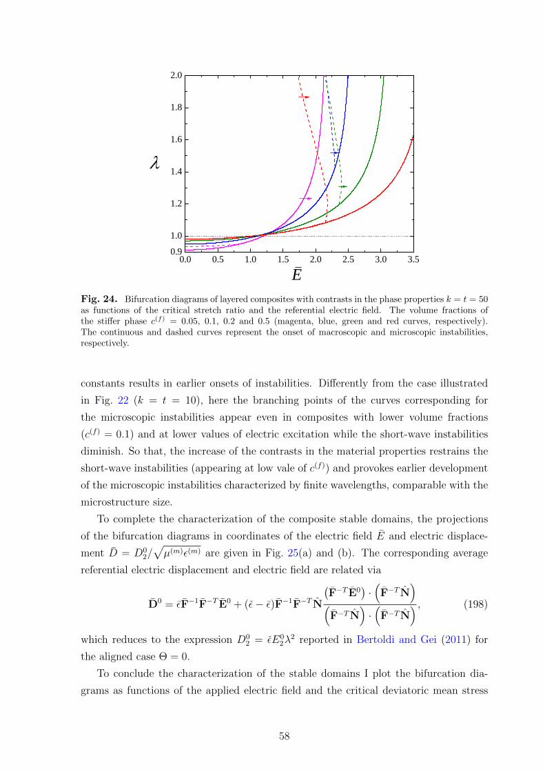
0 . 0 0 . 5 1 . 0 1 . 5 2 . 0 2 . 5 3 . 0 3 . 50 . 91 . 0
1 . 2
1 . 4
1 . 6
1 . 8
2 . 0
E
�
Fig. 24. Bifurcation diagrams of layered composites with contrasts in the phase properties k = t = 50as functions of the critical stretch ratio and the referential electric field. The volume fractions ofthe stiffer phase c(f) = 0.05, 0.1, 0.2 and 0.5 (magenta, blue, green and red curves, respectively).The continuous and dashed curves represent the onset of macroscopic and microscopic instabilities,respectively.
constants results in earlier onsets of instabilities. Differently from the case illustrated
in Fig. 22 (k = t = 10), here the branching points of the curves corresponding for
the microscopic instabilities appear even in composites with lower volume fractions
(c(f) = 0.1) and at lower values of electric excitation while the short-wave instabilities
diminish. So that, the increase of the contrasts in the material properties restrains the
short-wave instabilities (appearing at low vale of c(f)) and provokes earlier development
of the microscopic instabilities characterized by finite wavelengths, comparable with the
microstructure size.
To complete the characterization of the composite stable domains, the projections
of the bifurcation diagrams in coordinates of the electric field E and electric displace-
ment D = D02/√µ(m)ε(m) are given in Fig. 25(a) and (b). The corresponding average
referential electric displacement and electric field are related via
D0 = εF−1F−T E0 + (ε− ε)F−1F−T N
(F−T E0
)·(F−T N
)(F−T N
)·(F−T N
) , (198)
which reduces to the expression D02 = εE0
2λ2 reported in Bertoldi and Gei (2011) for
the aligned case Θ = 0.
To conclude the characterization of the stable domains I plot the bifurcation dia-
grams as functions of the applied electric field and the critical deviatoric mean stress
58

0 . 0 0 . 5 1 . 0 1 . 5 2 . 0 2 . 50
2
4
6
8
1 0
k = t = 1 0
E
D
( a )
0 . 0 0 . 5 1 . 0 1 . 5 2 . 0 2 . 5 3 . 00
2
4
6
8
1 0( b )
k = t = 5 0
E
D
Fig. 25. Bifurcation diagrams of layered composites with volume fractions of the stiffer phase
c(f) = 0.05, 0.1, 0.2 and 0.5 (magenta, blue, green and red curves, respectively) as functions of theelectric field E and electric displacement D. The continuous and dashed curves represent the onset ofmacroscopic and microscopic instabilities, respectively.
along the layers. These are shown in Fig. 26 for the same contrasts between the phase
properties, namely k = t = 10 in (a) and k = t = 50 in (b). Here, the mean deviatoric
stress is related to the stretch ratio and the electric field via
σD =1
3
((2− ε
µE2
)λ2 − 1− λ−2
). (199)
As anticipated on physical grounds, one can observe that the critical macroscopic
longitudinal stress is negative for relatively low applied electric fields. However, an
increase of the electric field impacts differently the critical mean stress depending on
the material morphology. In particular, for composites with higher contrasts in the
properties of the phases the critical stress increases (see Fig. 26(b)), while for composites
with lower contrasts the critical stress decreases when the volume fraction of the stiffer
phase is low (c(f) = 0.05 and 0.1 in Fig. 26(a)) and increases when c(f) is high (c(f) = 0.2
and 0.5 in Fig. 26(a)).
Consider the evolution of the stresses in the phases of the material along the equi-
librium path of a fixed pre-stretched configuration λ = 2. Shown in Fig. 27 are the
functions of the longitudinal deviatoric stresses in the phases and the applied electric
field. The red and blue curves correspond to the stresses in the stiffer and softer phases,
respectively, while the mean stresses are represented by the black curves. The dotted,
continuous and dashed curves correspond to the stresses along the equilibrium path,
and to the onset of macroscopic and microscopic instabilities, respectively. Along the
equilibrium path the stresses in the phases are positive at the initial pre-stretch config-
uration where E = 0, and an increase of the applied electric field leads to a decrease of
the stresses in the phases. Because of the different electric fields in the phases the stress
59

0 . 0 0 . 5 1 . 0 1 . 5 2 . 0 2 . 5- 1 . 5- 1 . 0- 0 . 50 . 00 . 51 . 01 . 5( a )
�
k = t = 1 0
EE
0 1 2 3 4- 0 . 2 50 . 0 00 . 2 50 . 5 00 . 7 51 . 0 01 . 2 5( b )
�
k = t = 5 0
EE
Fig. 26. Bifurcation diagrams of layered composites with volume fractions of the stiffer phase
c(f) = 0.05, 0.1, 0.2 and 0.5 (magenta, blue, green and red curves, respectively) as functions of thelongitudinal mean stress and the referential electric field. The continuous and dashed curves representthe onset of macroscopic and microscopic instabilities, respectively.
in the soft phase decreases faster and becomes negative. The difference in the deviatoric
longitudinal stresses increases as the electric field is increased and the equilibrium curves
intersect with the corresponding bifurcation curves.
The morphology significantly impacts the composite stability, restraining or pro-
moting different instability modes. To highlight this effect bifurcation diagrams are
presented as functions of the critical stretch ratio and the volume fraction of the stiffer
phase in Fig. 28. The failure surfaces are shown for composites with contrast ratios
k = t = 10 subjected to different electrical excitations E = 1.0, 1.6, 1.8 and 2.0 (red,
green, magenta and blue curves, respectively). The continuous and dashed curves cor-
respond to the onset of macroscopic and microscopic instabilities, respectively.
One can observe that for each unstable domain corresponding to a particular elec-
tric excitation three subdomains can be distinguished. The first corresponds to the one
where macroscopic instabilities (k1h→ 0) are identified. This macroscopically unstable
domain lies beneath the continuous curves. The domain increases with the increase
of the applied electric field. The second domain corresponds to a small zone at low
volume fractions of the stiffer phase, between the dashed and the continuous curves.
Here, instabilities associated with short waves (k1h→ 2π) appear. Differently from the
first domain, this one decreases with the increase of the electric excitation. So that the
applied electric field restrains the short-wave instabilities and stimulates the long-waves
instabilities. The above subdomains were observed for the purely mechanical case by
Triantafyllidis and Maker (1985). The peculiar third domain was not revealed in the
purely mechanical case. The characteristic scale of these instabilities is demonstrated in
60

0 . 0 0 . 4 0 . 8 1 . 2 1 . 6 2 . 0 2 . 2- 4
- 2
0
2
45
S t a b l e�����
� DM
k = t = 1 0
E
Fig. 27. The longitudinal stresses as functions of applied electric field of layered composites with
volume fraction of the stiffer phase c(f) = 0.5. The dotted, continuous and dashed curves correspondto the stresses along the equilibrium path λ = 2, onset of macroscopic and microscopic instabilities,respectively. The red curves represent the stresses in the stiffer phase and the blue ones correspond tothe stresses in the softer phase. The black curves represent the mean stresses.
Fig. 23 and it appears to be k1h ∼ 2. This domain is associated with high volume frac-
tion of the stiffer phase and large pre-stretches. When the electric excitation increases
the domain expands to include composites with moderate volume fractions at lower
levels of the stretch ratio. As the first and third domains expand towards each other as
the electric excitation increases, at some value of E they intersect. In the figure, I show
the distinguishing between them with the aid of the dotted curves.
It was shown by Geymonat et al. (1993) for the purely mechanical case that the long-
wave instabilities can be estimated from the loss of strong ellipticity of the corresponding
media. Furthermore, the macroscopic instability is an upper bound of the microscopic
instabilities. For the fully coupled electromechanical problem, I always observe this
phenomenon during calculation of the numerical examples (see, for example, Fig. 23).
The numerical results of Bertoldi and Gei (2011) for the aligned composites with some
specific volume fractions are also in agreement with those findings. In addition, I observe
that for the media with moderate volume fractions of the stiffer phase the macroscopic
instability can be used as a good estimate for the material failure.
Consider the influence of lamination angle Θ on the onset of instabilities. Noting
that at the lamination angles different from Θ = 0 and π/2 the microscopic instability
analysis becomes rather complicated and for the non-aligned loading cases I consider
61

0 . 0 0 . 2 0 . 4 0 . 6 0 . 8 1 . 00 . 5
1 . 0
1 . 5
2 . 0
2 . 5
3 . 0
c ( f )
�
Fig. 28. The failure surfaces of layered composites as functions of the critical stretch ratio andvolume fraction of the stiffer phase. The contrasts in the properties of the phases are k = t = 10.The red, green, magenta and blue curves correspond to E = 1.0, 1.6, 1.8 and 2.0, respectively. Thecontinuous and dashed curves correspond to the onset of the macroscopic and microscopic instabilities,respectively. The dotted curves separate the unified unstable domains according to the instability modeassociated with each part.
only the onset of macroscopic instabilities.
The bifurcation diagrams are presented in Fig. 29 as functions of the critical stretch
ratio and the volume fraction of the stiffer phase for composites with different lamination
angles Θ = 0, π/16, π/8 (blue, red and green continuous curves, respectively). The
composites are subjected to electric excitation E = 1.0 in Fig. 29(a) and E = 2.0 in
Fig. 29(b). In a manner reminiscent of the purely mechanical case (Triantafyllidis and
Maker, 1985), the macroscopic failure surfaces are symmetric with respect to c(f) = 0.5
and the composites are less stable in the range of moderate volume fraction of the stiffer
phase. Composites with volume fractions near c(f) ∼ 0 and 1 become stable. This effect
is intensified with an increase of the lamination angle, once again in a manner similar
to the one observed in laminated composites under mechanical loads (Nestorovic and
Triantafyllidis, 2004; Agoras et al., 2009a). An increase of the electric excitation results
in earlier onset of the macroscopic instability.
The picture alters drastically when the value of the electric field approaches E given
in Eq. (197). In contrast to the findings in Fig. 29(a), one can observe in Fig. 29(b) that
the composites with volume fractions of the stiffer phase in the vicinity of c(f) ∼ 0.144
and 0.856 become extremely unstable.
To highlight the transition of the composites behavior as the intensity of the electric
62

0 . 0 0 . 2 0 . 4 0 . 6 0 . 8 1 . 00 . 40 . 50 . 60 . 70 . 80 . 91 . 0( a )
�����
����
���
���
c ( f )
�
0 . 0 0 . 2 0 . 4 0 . 6 0 . 8 1 . 00 . 00 . 51 . 01 . 52 . 02 . 53 . 0( b )
���
�����
��
c ( f )
Fig. 29. The macroscopic failure surfaces of layered composites as functions of the stretch ratio andthe volume fraction of the stiffer phase. The contrasts in the properties of the phases are k = t = 10.(a) - E = 1.0; (b) - E = 2.0
field approaches the critical value of the applied electric field, the bifurcation diagrams of
composites with aligned layers (Θ = 0) are presented in Fig. 30 for E = 1.9, 1.925, 1.95,
1.975, 2.0 and 2.025 (blue, red, black, green, magenta and purple curves, respectively).
Thus, in contrast to the purely mechanical case where the most macroscopically unstable
morphology corresponds to c(f) = 0.5, in the electromechanical case the composite
behavior changes and the least stable volume fraction shifts. Remarkably, the results
of the numerical simulations hint that the dramatic change of the macroscopic curves
behavior may be associated with the unifying of the first and third unstable domains in
Fig. 28. At this stage, the media become unstable in a large range of c(f) (see Fig. 28).
One can observe that macroscopically, the effect of the lamination angle on the
composite stability varies from stabilization at low values of the electric fields to opposite
influence at high electric excitations. However, this trend might be different when
microscopic instabilities of shorter wave lengths are considered. Therefore, in following
examples I consider composites with volume fraction of the stiffer phase c(f) = 0.2 since
the macroscopic failure mode dominates at this morphology even at relatively high
electrostatic excitations.
Shown in Fig. 31 are the bifurcation diagrams for composites with c(f) = 0.2. The
bifurcation diagrams are presented as functions of the critical stretch ratio λ and the
referential electric field E. The contrasts in the properties of the phases are k = t = 10.
The lamination angles in the ranges 0 ≤ Θ ≤ π/4 and π/4 < Θ ≤ π/2 are presented in
Figs 31(a) and (b), respectively. The continuous curves correspond to the macroscopic
failure surfaces and the blue dashed curve in Fig. 31(a) represents the onset of the
microscopic instability for the aligned case (Θ = 0).
63

0 . 0 0 . 2 0 . 4 0 . 6 0 . 8 1 . 00 . 5
1 . 0
1 . 5
2 . 0
2 . 5
3 . 0
3 . 5
4 . 0
c ( f )
�
u n s t a b l e
Fig. 30. Failure surfaces of layered composites with Θ = 0 as functions of the stretch ratio andvolume fraction of the stiffer phase. The contrasts in the properties of the phases are k = t = 10. Theblue, red, black, green, magenta and purple curves correspond to E = 1.9, 1.925, 1.95, 1.975, 2.0 and2.025, respectively.
The corresponding expression for the critical stretch ratio takes a compact form
when Θ = π/2
λc =
(1− µ
µ− E2
(1− ε
ε
))−1/4
. (200)
In contrast to the aligned case (Θ = 0), here an increase of the applied electric field
stabilizes the media. It is easy to see from (200) that whenever the applied electric field
exceeds the value
Ec =
√(µ− µ)ε
(ε− ε)µ, (201)
the composite becomes macroscopically stable. For the composite with identical shear
to dielectric constants ratio of the phases r(f) = µ(f)/ε(f) = r(m) = µ(m)/ε(m) = r, this
value of the electric field is E0 (c)2 =
√r which corresponds to Ec = 1 (thin dashed line
in Fig. 31(b)).
In the pure mechanical case, the composites loose the stability only when the layers
are compressed in the lamination direction. If the composite is laminated at an angle
higher than a critical one, any applied compression will never lead to failure, since the
layers switch from compression to tension being rotated at angle π/4 in the deformed
configuration (Rudykh and deBotton, 2012). However, in the coupled electromechanical
case, when the electrostatic excitation is high enough even these composites may become
unstable. For instance, the composites with Θ = π/8 and Θ = π/4 are represented in
64

0 . 0 0 . 5 1 . 0 1 . 5 2 . 0 2 . 50 . 2
0 . 6
1 . 0
1 . 4
1 . 8
2 . 22 . 4( a )
����
� ��� �
��
���
E
�
0 . 0 0 . 5 1 . 0 1 . 5 2 . 01
2
3
4
5( b )
�����������
����
�����������
�����
E
�
Fig. 31. The bifurcation diagrams of layered composites with different lamination angles as functionof the critical stretch ratio and the referential electric field. The volume fraction of the stiffer phase isc(f) = 0.2 and the contrasts in the properties of the phases are k = t = 10. (a) - small angles; (b) -large angles
Fig. (31) by the pink and purple curves, respectively. While in the pure mechanical
case, the failure surfaces possess the property λ(Θ) = 1/λ(Θ +π/2), the failure surfaces
of the coupled problem do not.
In the limiting cases Θ = 0 and Θ = π/2 I note the different role of the electric
field, which is to stimulate instabilities in the first case while stabilizing in the second.
The behaviors of composites with intermediate angles of lamination are associated with
transition between the limiting cases (from Θ = 0 to Θ = π/2) as the role of the electric
field is concerned. Obviously, at some lamination angle in the deformed configuration
the role of the electric field switches.
This is illustrated in Fig. (32) as a conclusive example for the composite with sim-
ilar to the previously considered material properties and volume fraction of the stiffer
phase. The diagrams show the dependence of the critical stretch ratio on the lami-
nation angle. The black, bright green, orange, green, magenta, blue and red curves
correspond to applied electric excitations E = 0.0, 0.5, 1.0, 1.5, 1.8, 1.9 and 2.0, respec-
tively. The bifurcation diagrams are symmetric with respect to 0 and π/2 and periodic
in π. In agreement with the previous discussion, at low lamination angles the electric
field promotes instabilities, whereas at the lamination angles close to π/2 the applied
electric field stabilizes the composites. Due to this stabilization effect in composites
with lamination angles close to π/2, instabilities may occur only under relatively low
electric fields (E < 1). One can observe that for moderate levels of the electric field
(e.g., E = 1.5 and E = 1.8) there are two disjoint unstable domains. The first contains
the aligned composite (Θ = 0) and the other includes composites with larger lamination
angles at large critical stretch ratios. Composites with lamination angles between these
65

0 . 0 0 . 1 0 . 2 0 . 3 0 . 4 0 . 50 . 0
0 . 5
1 . 0
1 . 5
2 . 0
2 . 5
3 . 0
���
���
���
��� ���
���
������
c ( f ) = 0 . 2��
���
���
����
���
Fig. 32. Bifurcation diagrams as functions of the stretch ratio and lamination angle. The contrastsin properties of the phases are k = t = 10.
two domains are stable materials at these levels of excitations (e.g., composites with
0.11π < Θ < 0.3π for E = 1.5). With increase of the electric field the unstable domains
near one to another. That continues up to a certain value of the electric field is achieved
at which the two domains unite (e.g., the transition from E = 1.8 to E = 1.9). Beyond
this value of the electric field the only stable morphology is the one with Θ = π/2.
Remarkably, the value of the electric field at which the domains unite corresponds to
the situation where the influence of lamination angles switches from stabilization to the
opposite one.
Note that for the composites with isotropic phases in the cases Θ = nπ, π/2 + nπ,
where n = 0, 1, 2..., coefficients Γ1, Γ3, Γ5 vanish in the polynomial equation (170) and
the condition for ellipticity loss can be written in terms of the bi-cubic polynomial
Γ6ξ6 + Γ4ξ
4 + Γ2ξ2 + Γ0 = 0. (202)
Analogous results in terms of the nominal electric displacement instead of the referential
electric field, were reported by Dorfmann and Ogden (2010) for surface instabilities in
half space isotropic dielectrics and by Bertoldi and Gei (2011) for long wave instabilities
in layered composites with isotropic phases and lamination angle Θ = 0.
66

4.3 Concluding Remarks
A systematic study of the multiscale instabilities in soft composite dielectrics was con-
ducted in terms of physically relevant variables. First, a general criterion for onset of
instabilities associated with long waves was introduced. Second, a condition for the on-
set of microscopic instability was introduced for the layered composites with anisotropic
phases. Third, a closed form expression for energy-density function of these media is de-
duced. This allowed us to detect that whenever the medium fails it occurs in one of the
three unstable domains depending on the composite morphology and electromechanical
loadings
(i) long-wave instabilities dominate at moderate volume fractions of the stiffer phase
(ii) interface instabilities appear at low volume fractions of the stiffer phase
(iii) instabilities of microstructure characteristic scales occur at high volume fractions
of the stiffer phase
An increase of electric field suppresses the (ii)-type of instabilities and promotes the
(i)- and (iii)- types. Thus, the unstable domains of the long and finite waves unite
and create a new unstable domain. At this point the composite becomes extremely
unstable at a large variety of its morphologies. This critical point can be detected by
a more compact analysis of macroscopic instabilities only. Whenever the macroscopic
failure surfaces alters drastically in the illustrated way, the critical situation is achieved.
These can be strictly determined from the closed form expressions for critical values
of the pre-stretch depending on the applied electric fields. Thanks to these analytical
expressions the critical values of the electric fields are revealed
1. composites with lamination angle Θ = 0 lose the stability whenever electric exci-
tation exceeds the value given in (197)
2. composites with lamination angle Θ = π/2 become macroscopically stable when-
ever electric excitation exceeds the value given in (201)
Based on the macroscopic analysis it is found that at low values of the electric
field an increase of lamination angles stabilizes the media and has an opposite effect at
high electric fields. The transition between these opposite influences occurs when two
macroscopically unstable domains meet and unite.
67

Chapter 5
Thick-Wall EAP Balloon
A major limitation of EAP originates in the need for relatively large electric fields. How-
ever, usage of instability phenomena (Mockensturm and Goulbourne, 2006; Dorfmann
and Ogden, 2010) may reduce the intensity of the required electric field. Accordingly,
I analyze the response of EAP balloons and demonstrate that a relatively small elec-
trostatic field can be used as a trigger for large deformations. I follow the theory of
nonlinear electroelasticity by Toupin (1956); McMeeking and Landis (2005), where the
total stress is
σ(t)ij = σ
(c)ij + σ
(m)ij . (203)
Here, σ(c)ij is the Cauchy mechanical stress, σ
(m)ij = εε0EiEj − ε0
2EnEnδij is the Maxwell
stress induced by the electric field E, ε is a dielectric modulus, and ε0 is the vacuum
permittivity. Assume that ε = 6, which is typical for common polymers, is constant. I
adopt a quite general constitutive law for incompressible isotropic materials, in which
the principal stresses are
σ(c)k =
N∑p=1
µpλαp
k − q, (204)
where λk are the principal stretches, q is an arbitrary hydrostatic pressure, µp are
shear moduli, and αp are material constants. In the case N = 1 with α1 = 2, the
model (204) which is commonly denoted Ogden model, reduces to the neo-Hookean
one. With N = 3 an excellent correlation with experimental data for elastomers is
revealed (Treloar, 1975). Accordingly, I assume the following typical values for the
elastic constants of soft polymers (Treloar, 1975) µ1 = 6.3 · 105Pa, µ2 = 1.2 · 103Pa,
µ3 = −1 · 104Pa, α1 = 1.3, α2 = 5, and α3 = −2. In the vicinity of the reference
configuration this polymer behaves like a neo-Hookean material with shear modulus
µ = 12
∑3p=1µpαp = 4.225 · 105Pa.
Consider a spherical balloon made out of a dielectric elastomer with inner Ri and
outer Ro radii. Here and thereafter, the notations (•)i and (•)o are used to specify
quantities at the inner and outer radii, respectively. The thickness of the balloon wall
is H = Ro −Ri. The inner and outer surfaces of the balloon wall are covered with thin
electrodes with negligible elastic modulus (Bhattacharya et al., 2001) that enable to
induce an electric field across the wall. The balloon can be inflated with inner pressure
68
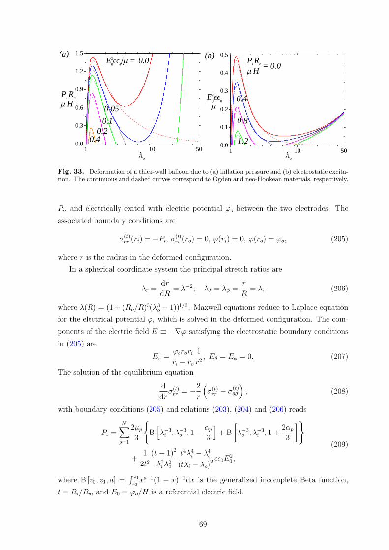
1 10 500.0
0.3
0.6
0.9
1.2
1.5(a)
�� H
�o
0.40.2
0.10.05
E20��
���� �= 0.0
Pi Ro
1 10 500.0
0.1
0.2
0.3
0.4
0.5(b)
�o
0.8
= 0.0�� H
�
1.2
0.4E20��
��
Pi Ro
Fig. 33. Deformation of a thick-wall balloon due to (a) inflation pressure and (b) electrostatic excita-tion. The continuous and dashed curves correspond to Ogden and neo-Hookean materials, respectively.
Pi, and electrically exited with electric potential ϕo between the two electrodes. The
associated boundary conditions are
σ(t)rr (ri) = −Pi, σ(t)
rr (ro) = 0, ϕ(ri) = 0, ϕ(ro) = ϕo, (205)
where r is the radius in the deformed configuration.
In a spherical coordinate system the principal stretch ratios are
λr =dr
dR= λ−2, λθ = λφ =
r
R= λ, (206)
where λ(R) = (1 + (Ro/R)3(λ3o − 1))1/3. Maxwell equations reduce to Laplace equation
for the electrical potential ϕ, which is solved in the deformed configuration. The com-
ponents of the electric field E ≡ −∇ϕ satisfying the electrostatic boundary conditions
in (205) are
Er =ϕororiri − ro
1
r2, Eθ = Eφ = 0. (207)
The solution of the equilibrium equation
d
drσ(t)rr = −2
r
(σ(t)rr − σ
(t)θθ
), (208)
with boundary conditions (205) and relations (203), (204) and (206) reads
Pi =N∑p=1
2µp3
{B[λ−3i , λ−3
o , 1− αp3
]+ B
[λ−3o , λ−3
i , 1 +2αp3
]}
+1
2t2(t− 1)2
λ2iλ
2o
t4λ4i − λ4
o
(tλi − λo)2 εε0E20 ,
(209)
where B [z0, z1, a] =∫ z1z0xa−1(1 − x)−1dx is the generalized incomplete Beta function,
t = Ri/Ro, and E0 = ϕo/H is a referential electric field.
69

1 10 200.0
0.4
0.8
1.2
1.6
2.0
0.9
0.8
�� H
0.99
t = 0.6
E20��
���� = 0.01
�
Pi Ro
Fig. 34. The deformations of balloons with different wall thicknesses as functions of the pressurewith fixed electric excitation. The dashed curve corresponds to the thin-wall approximation (210).
Results for a thick-wall balloon (t = 0.8) are presented in Fig. 33. Shown in Fig. 33a
is the inflation pressure versus the stretch ratio for a few fixed electric fields. Fig. 33b
shows the electric field versus the stretch ratio for a few values of the inflation pressure.
The results for the Ogden and the neo-Hookean materials are denoted by continuous
and dashed curves, respectively.
With the increase of the inflation pressure the balloon slowly expands until a critical
pressure is reached. Further increase in the pressure leads to a sudden jump in the size
of the balloon to a new stable state. This phenomenon is commonly denoted “snap-
through”. Application of electric field reduces the critical pressure at which the balloon
snaps. One can observe that this effect cannot be recovered with the neo-Hookean
material (Zhu et al., 2010). Similarly, electrostatic excitation which is applied in the
undeformed configuration leads to expansion of the balloon up to a critical electric field.
Further increase in the electric potential results in a snap-through of the balloon. When
applied to a pre-inflated balloon, the critical electric field at which the instability occurs
decreases. Note that after instability occurs, the slopes of the curves decrease. This
implies that once the balloon snaps to its new state, smaller variations in the electric
field result in larger actuations.
For thin-wall spheres (Mockensturm and Goulbourne, 2006) Eq. (209) can be sim-
plified to
Pi =2H
R
(N∑p=1
µp(λαp−3 − λ−2αp−3
)− ε0εE2
0λ
). (210)
70
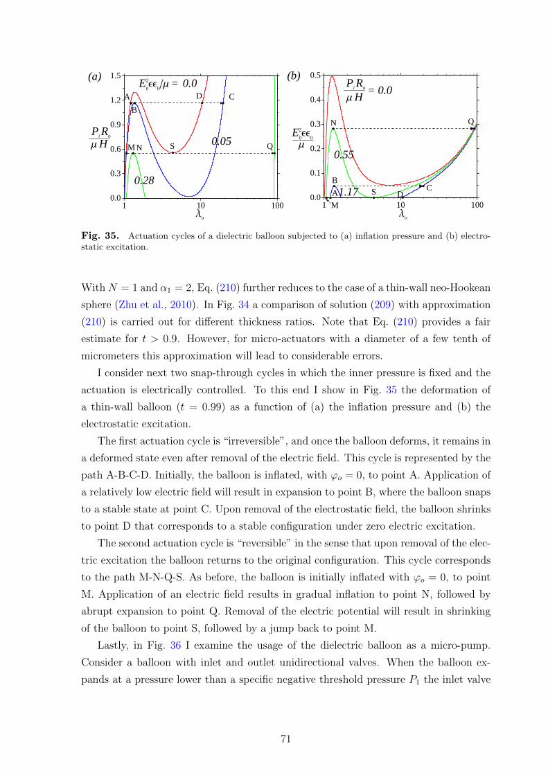
1 10 1000.0
0.3
0.6
0.9
1.2
1.5(a)
S
D
M N Q
B
�� H
CA
�o
0.28
0.05
E20��
���� �= 0.0
Pi Ro
1 10 1000.0
0.1
0.2
0.3
0.4
0.5(b)
SB
QN
M
CDA
�o
0.55
= 0.0�� H
�
1.17
E20��
��
Pi Ro
Fig. 35. Actuation cycles of a dielectric balloon subjected to (a) inflation pressure and (b) electro-static excitation.
With N = 1 and α1 = 2, Eq. (210) further reduces to the case of a thin-wall neo-Hookean
sphere (Zhu et al., 2010). In Fig. 34 a comparison of solution (209) with approximation
(210) is carried out for different thickness ratios. Note that Eq. (210) provides a fair
estimate for t > 0.9. However, for micro-actuators with a diameter of a few tenth of
micrometers this approximation will lead to considerable errors.
I consider next two snap-through cycles in which the inner pressure is fixed and the
actuation is electrically controlled. To this end I show in Fig. 35 the deformation of
a thin-wall balloon (t = 0.99) as a function of (a) the inflation pressure and (b) the
electrostatic excitation.
The first actuation cycle is “irreversible”, and once the balloon deforms, it remains in
a deformed state even after removal of the electric field. This cycle is represented by the
path A-B-C-D. Initially, the balloon is inflated, with ϕo = 0, to point A. Application of
a relatively low electric field will result in expansion to point B, where the balloon snaps
to a stable state at point C. Upon removal of the electrostatic field, the balloon shrinks
to point D that corresponds to a stable configuration under zero electric excitation.
The second actuation cycle is “reversible” in the sense that upon removal of the elec-
tric excitation the balloon returns to the original configuration. This cycle corresponds
to the path M-N-Q-S. As before, the balloon is initially inflated with ϕo = 0, to point
M. Application of an electric field results in gradual inflation to point N, followed by
abrupt expansion to point Q. Removal of the electric potential will result in shrinking
of the balloon to point S, followed by a jump back to point M.
Lastly, in Fig. 36 I examine the usage of the dielectric balloon as a micro-pump.
Consider a balloon with inlet and outlet unidirectional valves. When the balloon ex-
pands at a pressure lower than a specific negative threshold pressure P1 the inlet valve
71

1 10 100 200-0.6
-0.3
0.0
0.3
0.6
0.9
1.2
1.5
1 1.1 1.2 1.3 1.4 1.5-0.6
-0.3
0.0
0.3
0.6
0.9
1.2
1.5
CB
A
(a)
D
A
B
C
�� HE
�o
0.34
0.61E2
0��
���� �= 0.0
Pi Ro
� H
Pi Ro
�o
1 10 100 2000.0
0.2
0.4
0.6
1 1.1 1.2 1.3 1.4 1.50.0
0.1
0.2
0.3
0.4
0.5
0.6 C
A
B
(b) DC
B
A
F
�o
0.4 = 0.0
�� H
�
-0.29
E20��
��
Pi Ro
�E2
0��
��
�o
Fig. 36. Pumping cycle of a dielectric balloon subjected to (a) inflation pressure and (b) electrostaticexcitation.
opens and allows liquid to flow into the balloon. When the balloon shrinks, at some
positive threshold pressure P2 the outlet valve opens and liquid flows out. In a way of
an example, in Fig. 36 the normalized pressures are P1 = −0.29 and P2 = 0.4. The
pumping cycle starts at point A at which the internal pressure is slightly lower than P2.
Once the balloon is excited, due to the electrostatic forces that act to shrink its wall, the
internal pressure drops to P1 at constant λ (since the balloon cannot deform as long as
both valves are close). At this point the inlet valve opens, and the balloon expands while
liquid flows in (segment B-C). At point C, due to the instability, the balloon further
expands to point D. This is a stable point at which the inlet valve closes, terminating
the sucking stage. As the electric excitation is removed, due to the elasticity of the
balloon the inner pressure increases as long as the pressure is lower than P2 (segment
D-E). At point E the pressure reaches P2, the outlet valve opens and liquid flows out of
the balloon as it starts to shrink. This process continues till the balloon returns back
to point A through point F.
72

Conclusions
This thesis concerns multiscale instabilities in electroactive composites undergoing fi-
nite deformations. First, large scale or macroscopic instabilities were considered. In the
context of the purely mechanical problem, the onset of macroscopic instability is de-
tected when the governing incremental equations loose the ellipticity and bifurcations of
the solution occur. This idea together with the implementation of the micromechanical
approach to composites with random distribution of aligned fibers, resulted in a closed
form compact expression for the critical stretch ratio of composites with neo-Hookean
and Gent constituents. These analytical findings were fairly compared with the 3-D FE
simulations for which an instability analysis algorithm was developed in the framework
of finite deformation elasticity.
A general criterion for the onset of macroscopic electromechanical instabilities was
derived. This can be utilized for identification of the instability onset even in multiphase
composites. Since possible application of electroactive materials are controlled by the
applied voltage, an approach involving the referential electric field as a primary variable
was adopted. Furthermore, a similar electromechanical instability criterion was derived
in terms of the referential electric displacement as a primary variable. By application
of the criterion to a class of layered anisotropic materials for which an exact analytical
solution was derived, the unstable domains were revealed. It was found that the electric
excitation promotes instabilities if applied perpendicular to the layers. If the electric
excitation is parallel to the layers the composite is stabilized. Generally, an increase
of the pre-stretch in the layers direction stabilizes the media. Remarkably, when the
physically relevant approach of the referential electric field as a primary variable is
utilized important stability properties are recovered, most of them cannot be predicted
by the convenient formulation in terms of the electric displacement. For instance, there
are electric fields beyond which the composites become unstable regardless of the pre-
stretch, whereas for every value of the applied electric displacement there exists a pre-
stretch for which the composite remains stable. Depending on the contrast between
the phase properties, extremely unstable morphologies can be found. Once again, these
cannot be detected when analysis in terms of the electric displacement is adopted.
The core of the work is the analysis of electromechanical microscopic instabilities.
A condition for the onset of microscopic instabilities was derived by application of
Bloch-Floquet technique to periodic layered structure with general anisotropic phases.
73

This allowed to detect that whenever the layered medium fails, it occurs in one of the
three unstable domains depending on the composite morphology and electromechanical
loadings
(i) long-wave instabilities dominate at moderate volume fractions of the stiffer phase
(ii) interface instabilities appear at low volume fractions of the stiffer phase
(iii) instabilities of microstructure characteristic scales occur at high volume fractions
of the stiffer phase
The results for the first mode of instabilities agree with the ones obtained from the
general criterion for the macroscopic instabilities. Whereas the first and second modes
of instabilities were detected in the purely mechanical case, the third mode is unique
and appears only in the coupled case. These domains evolve with changes in the applied
electric field such that the overall unstable domain increases when the electric field is
increased.
Finally, a possible application of the instability phenomenon in thick wall spheri-
cal balloon was examined. To this end an exact analytical solution was derived and
actuation mechanisms for micro-pumps were proposed.
74

Appendix A
Kinematic tensors of the TI invariants
The explicit expressions for the kinematic tensors of the physically motivated invariants
are∂λ2
n
∂F= 2FN⊗ N, (A.1)
∂λ2p
∂F= λ2
pF−T −
λ2p
λ2n
FN⊗ N, (A.2)
∂γ2n
∂F=
2
λ2n
(FN⊗CN + FCN⊗ N)− 2(γ2
n
λ2n
+ 2)FN⊗ N (A.3)
and
∂γ2p
∂F= 2F− 2λ2
pF−T + 2
(γ2n + λ2
p
λ2n
+ 1)FN⊗ N− 2
λ2n
(FN⊗CN + FCN⊗ N). (A.4)
75

Appendix B
Kinematic tensors of the electromechanical
invariants
∂I1
∂Fij= 2Fij (B.1)
∂2I1
∂Fij∂Fkl= 2δikδjl, (B.2)
∂I5e
∂Fpq= −2C−1
qj E0jF−1ip E
0i , (B.3)
∂I5e
∂E0i
= 2C−1ij E
0j (B.4)
∂2I5e
∂Fpq∂Fkl= 2{C−1qj E
0jF−1ik E
0i F−1lp +
(C−1li E
0i F−1qk + F−1
ik E0i C−1lq
)F−1jp E
0j
}, (B.5)
∂2I5e
∂Fpq∂E0k
= −2(C−1qj E
0jF−1kp + C−1
qk E0jF−1jp
), (B.6)
∂2I5e
∂E0i ∂E
0j
= 2C−1ij , (B.7)
∂C−1ij
∂Fpq= −C−1
qj F−1ip − C−1
qi F−1jp . (B.8)
76

Appendix C
R-Matrix of the electromechanical
instability analysis
The non-zero entries of R can be written as
R11 = k21b(G122(G122 + G221 − G111)− (A1122 +A1221 −A1111)E22
),
R12 = k21b (A1121E22 − G121G122) , R13 = −ik1b
(G111E22 + G122E11
),
R14 = ik1b(
2G122 − (G112 + G121)E22E12
), R15 = ik1bE22,
R16 = ik1b(G122(G112 + G121 − G222)− (2A1112 −A1222)E22
)R21 = bk2
1E−122 (G2
122 −A1212E22)(
(A1121 − 2A2122)E22 + G222(G122 + G221 − G111))−
(A1222 − E−122 G122G222)R11,
R22 = −k21
{b(G122(A1222G121 +A1121G222)−A1121A1222E22 −A1212G121G222
)+A2121
},
R23 = ik1
{G121 −
(A1222E22G111 + (A1212G222 −A1222G122)E11
)b},
R24 = −ik1
{(E22A1222(G112 + G121)− 2E12(A1222G122 +A1212G222)− G122(G112 + G121)G222
)b+
G122 + G221
}, R25 = ik1b(A1222E22 − G122G222),
R26 = −ik1E−122
{((2A1112 −A1222)E22 − G122(G112 + G121 − G222)
)(A1222E22 − G122G222)b−
(A1122 +A1221 −A2222)E22 − (G112 + G121 − G222)G222
},
R31 = k21b(
(A1111 −A1122 −A1221)G122 +A1212(G122 + G221 − G111)),
R32 = k21b(A1212G121 −A1121G122
), R33 = ik1b
(G111G122 −A1212E11
),
R34 = ik1b(
(G112 + G121)G122 −A1212E12
), R35 = −ik1bG122,
R36 = −ik1b(
(A1222 − 2A1112)G122 +A1212(G112 + G121 − G222)),
R41 = −ik1, R54 = ik1, R66 = 1. (C.1)
where b = (A1212E22 − G2122)
−1.
77

Bibliography
Agoras, M., Lopez-Pamies, O. and Ponte Castaneda, P. (2009a). A general hyperelastic model
for incompressible fiber-reinforced elastomers, J. Mech. Phys. Solids 57: 268–286.
Agoras, M., Lopez-Pamies, O. and Ponte Castaneda, P. (2009b). Onset of macroscopic insta-
bilities in fiber-reinforced elastomers at finite strain, J. Mech. Phys. Solids 57: 1828–1850.
Aravas, N., Cheng, C. and Ponte Castaneda, P. (1995). Steady-state creep of fiber-reinforced
composites: Constitutive equations and computational issues, Int. J. Solids Structures
32: 2219–2244.
Bar-Cohen, Y. (2001). EAP history, current status, and infrastructure, in Y. Bar-Cohen (ed.),
Electroactive Polymer (EAP) Actuators as Artificial Muscles, SPIE press, Bellingham, WA,
chapter 1, pp. 3–44.
Bertoldi, K. and Boyce, M. C. (2008). Wave propagation and instabilities in monolithic and
periodically structured elastomeric materials undergoing large deformations, Phys. Rev. B
78: 184107.
Bertoldi, K. and Gei, M. (2011). Instabilities in multilayered soft dielectrics, J. Mech. Phys.
Solids 59: 18–42.
Bhattacharya, K., Li, J. Y. and Xiao, Y. (2001). Electromechanical models for optimal de-
sign and effective behavior of electroactive polymers, in Y. Bar-Cohen (ed.), Electroactive
Polymer (EAP) Actuators as Artificial Muscles, SPIE press, chapter 12, pp. 309–330.
Biot, M. A. (1965). Mechanics of Incremental Deformations, John Wiley and Sons, New-York.
Budiansky, B. (1983). Micromechanics, Computers & Structures 16: 3–12.
Carpi, F. and DeRossi, D. (2005). Improvement of electromechanical actuating performances of
a silicone dielectric elastomer by dispersion of titanium dioxide powder, IEEE Transactions
on Dielectrics and Electrical Insulation 12(4): 835–843.
Carpi, F., Salaris, C. and De Rossi, D. (2007). Folded dielectric elastomer actuators, Smart
Materials & Structures 16: 300–305.
78

deBotton, G. (2005). Transversely isotropic sequentially laminated composites in finite elas-
ticity, J. Mech. Phys. Solids 53: 1334–1361.
deBotton, G. (2008). Composites with one and two families of fibers, Presented at the Com-
posites and Polycrystals Mini-Symposium at the SIAM conference on Mathematical aspects
of materials science, Philadelphia, PA.
deBotton, G. and Hariton, I. (2006). Out-of-plane shear deformation of a neo-Hookean fiber
composite, Physics Letters A 354: 156–160.
deBotton, G., Hariton, I. and Socolsky, E. A. (2006). Neo-Hookean fiber-reinforced composites
in finite elasticity, J. Mech. Phys. Solids 54: 533–559.
deBotton, G. and Schulgasser, K. (1996). Bifurcation of orthotropic solids, J. Appl. Mech.,
Trans. ASME 63: 317–320.
deBotton, G. and Shmuel, G. (2009). Mechanics of composites with two families of finitely
extensible fibers undergoing large deformations, J. Mech. Phys. Solids 57: 1165–1181.
deBotton, G. and Shmuel, G. (2010). A new variational estimate for the effective response of
hyperelastic composites, J. Mech. Phys. Solids 58: 466–483.
deBotton, G. and Tevet-Deree, L. (2006). Electroactive polymer composites - analysis and sim-
ulation, in W. D. Armstrong (ed.), Smart Structures and Materials 2006: Active Materials:
Behavior and Mechanics, Vol. 6170 of Proc. of SPIE, San Diego, CA, pp. 2401–2410.
deBotton, G., Tevet-Deree, L. and Socolsky, E. A. (2007). Electroactive heterogeneous poly-
mers: analysis and applications to laminated composites, Mechanics of Advanced Materials
and Structures 14: 13–22.
Dorfmann, A. and Ogden, R. W. (2005). Nonlinear electroelasticity, Acta. Mech. 174: 167–183.
Dorfmann, A. and Ogden, R. W. (2010). Nonlinear electroelastostatics: Incremental equations
and stability, International Journal of Engineering Science 48: 1–14.
Ericksen, J. L. and Rivlin, R. S. (1954). Large elastic deformations of homogeneous anisotropic
materials, Arch. Rational. Mech. Anal. 3: 281–301.
Fleck, N. (1997). Compressive failure of fiber composites, Advances in Applied Mechanics
33: 43–117.
Gei, M., Roccabianca, S. and Bacca, M. (2010). Controlling band gap in electroactive polymer-
based structures, IEEE-ASME Transactions on Mechatronics (in press) .
Gent, A. N. (1996). A new constitutive relation for rubber, Rubber Chemistry and Technology
69: 59–61.
79

Geymonat, G., Muller, S. and Triantafyllidis, N. (1993). Homogenization of nonlinearly elas-
tic materials, microscopic bifurcation and macroscopic loss of rank-one convexity, Arch.
Rational. Mech. Anal. 122: 231–290.
He, Q. C., Le Quang, H. and Feng, Z. Q. (2006). Exact results for the homogenization of
elastic fiber-reinforced solids at finite strain, J. of Elasticity 83: 153–177.
Hill, R. (1972). On constitutive macro-variables for heterogeneous solids at finite strain, Proc.
R. Soc. Lond. A 326: 131–147.
Hill, R. and Hutchinson, J. W. (1975). Bifurcation phenomena in the plane tension test, J.
Mech. Phys. Solids 23: 239–264.
Horgan, C. and Saccomandi, G. (2002). A molecular-statistical basis for the gent constitutive
model of rubber elasticity, J. of Elasticity 68: 167–176.
Huang, C. and Zhang, Q. M. (2004). Enhanced dielectric and electromechanical responses in
high dielectric constant all-polymer percolative composites, adv. func. mater. 14: 501–506.
Huang, C., Zhang, Q. M., deBotton, G. and Bhattacharya, K. (2004). All-organic dielectric-
percolative three-component composite materials with high electromechanical response, Ap-
plied Physics Letters 84: 4391–4393.
Khisaeva, Z. and Ostoja-Starzewski, M. (2006). On the size of rve in finite elasticity of random
composites, J. of Elasticity 85: 153–173.
Kittel, C. (2004). Introduction to Solid State Physics, 8 edn, Wiley.
Kofod, G., Sommer-Larsen, P., Kornbluh, R. and Pelrine, R. (2003). Actuation response of
polyacrylate dielectric elastomers, Journal of Intelligent Material Systems and Structures
14: 787–793.
Lacour, S.-P., Prahlad, H., Pelrine, R. and Wagner, S. (2004). Mechatronic system of dielec-
tric elastomer actuators addressed by thin film photoconductors on plastic, Sensors and
actuators A-physical 111: 288–292.
Liu, L., Liu, Y., Zhang, Z., Li, B. and Leng, J. (2010). Electromechanical stability of electro-
active silicone filled with high permittivity particles undergoing large deformation, Smart
Materials & Structures 19(11).
Lopez-Pamies, O. and Idiart, M. (2010). Fiber-reinforced hyperelastic solids: a realizable
homogenization constitutive theory, J. of Engineering Mathematics 68: 57–83.
Lopez-Pamies, O. and Ponte Castaneda, P. (2004). Second-order estimates for the macroscopic
response and loss of ellipticity in porous rubbers at large deformations, J. of Elasticity
76: 247–287.
80

McMeeking, R. M. and Landis, C. M. (2005). Electrostatic forces and stored energy for
deformable dielectric materials, J. Appl. Mech., Trans. ASME 72: 581–590.
Merodio, J. and Ogden, R. W. (2002). Material instabilities in fiber-reinforced nonlinearly
elastic solids under plane deformation, Archives of Mechanics (IPPT) 54: 525–552.
Merodio, J. and Pence, T. J. (2001). Kink surfaces in a directionally reinforced neo-hookean
material under plane deformation: Ii. kink band stability and maximally dissipative band
broadening, J. of Elasticity V62(2): 145–170.
Michel, J. C., Lopez-Pamies, O., Castaneda, P. P. and Triantafyllidis, N. (2007). Microscopic
and macroscopic instabilities in finitely strained porous elastomers, J. Mech. Phys. Solids
55: 900–938.
Mockensturm, E. M. and Goulbourne, N. (2006). Dynamic response of dielectric elastomers,
Int. J. Nonlinear Mech. 41: 388 – 395.
Molberg, M., Crespy, D., Rupper, P., Nueesch, F., Manson, J., Loewe, C. and Opris, D. (2010).
High Breakdown Field Dielectric Elastomer Actuators Using Encapsulated Polyaniline as
High Dielectric Constant Filler, Advanced Functional Materials 20(19): 3280–3291.
Moraleda, J., Segurado, J. and LLorca, J. (2009). Finite deformation of incompressible fiber-
reinforced elastomers: a computational micromechanics approach, J. Mech. Phys. Solids
57: 1596–1613.
Nestorovic, M. D. and Triantafyllidis, N. (2004). Onset of failure in finitely strained layered
composites subjected to combined normal and shear loading, J. Mech. Phys. Solids 52: 941–
974.
Ogden, R. W. (1974). On the overall moduli of non-linear elastic composite materials, J.
Mech. Phys. Solids 22: 541–553.
Ogden, R. W. (1997). Non-Linear Elastic Deformations, Dover Publications, New York.
Ogden, R. W. (2008). Nonlinear elasticity and fibrous structure in arterial wall mechanics,
Lecture Notes for Summer School on Modeling and Computation in Biomechanics, Graz
University of Technology, Austria.
O’Halloran, A., O’Malley, F. and McHugh, P. (2008). A review on dielectric elastomer actua-
tors, technology, applications, and challenges, J. Appl. Phys. 104: 071101.
Pelrine, R., Kornbluh, R., Pei, Q.-B. and Joseph, J. (2000). High-speed electrically actuated
elastomers with strain greater than 100%, Science 287: 836–839.
81

Plante, J.-S. and Dubowsky, S. (2006). Large-scale failure modes of dielectric elastomer actu-
ators, Int. J. Solids Struct. 43: 7727–7751.
Qiu, G. and Pence, T. (1997). Loss of ellipticity in plane deformation of a simple directionally
reinforced incompressible nonlinearly elastic solid, J. of Elasticity 49: 31–63.
Rosen, B. W. (1965). Mechanics of composite strengthening, Fibre Composite Materials, Am.
Soc. Metals, Ohio, pp. 37–75.
Rudykh, S., Bhattacharya, K. and deBotton, G. (2012a). Multiscale instabilities in soft het-
erogeneous dielectrics.
Rudykh, S., Bhattacharya, K. and deBotton, G. (2012b). Snap-through actuation of thick-wall
electroactive balloons, Int. J. Nonlinear Mech. 47: 206–209.
Rudykh, S. and deBotton, G. (2011). Stability of anisotropic electroactive polymers with
application to layered media, Z. Angew. Math. Phys. 62: 1131–1142.
Rudykh, S. and deBotton, G. (2012). Instabilities of hyperelastic fiber composites: microme-
chanical versus numerical analyses, J. of Elasticity 106: 123–147.
Rudykh, S., Lewinstein, A., Uner, G. and deBotton, G. (2011). Giant enhancement of the
electromechanical coupling in soft heterogeneous dielectrics, Arxiv preprint arxiv:1105.4217
.
URL: http://arxiv.org/abs/1105.4217v1
Shmuel, G. and deBotton, G. (2010). Out-of-plane shear of fiber composites at moderate
stretch levels, J. of Engineering Mathematics 68: 85–97.
Singamaneni, S., Bertoldi, K., Chang, S., Jang, J., Young, S. L., Thomas, E. L., Boyce, M. C.
and Tsukruk, V. V. (2009). Bifurcated Mechanical Behavior of Deformed Periodic Porous
Solids, Advanced Functional Materials 19(9): 1426–1436.
Stoyanov, H., Kollosche, M., Risse, S., McCarthy, D. and Kofod, G. (2011). Elastic block
copolymer nanocomposites with controlled interfacial interactions for artificial muscles with
direct voltage control, Soft Matter 7(1): 194–202.
Suo, Z., Zhao, X. and Greene, W. H. (2008). A nonlinear field theory of deformable dielectrics,
J. Mech. Phys. Solids 56(2): 467–486.
Tevet-Deree, L. (2008). Electroactive Polymer Composites - Analysis and Simulation, PhD
thesis, Ben-Gurion University.
Tian, L., Tevet-Deree, L., deBotton, G. and Bhattacharya, K. (2012). Dielectric elastomer
composites, J. Mech. Phys. Solids 60: 181–198.
82

Toupin, R. A. (1956). The elastic dielectric, Arch. Rational. Mech. Anal. 5: 849–915.
Treloar, L. R. G. (1975). The Physics of Rubber Elasticity, Clarendon Press, Oxford.
Triantafyllidis, N. and Maker, B. N. (1985). On the comparison between microscopic and
macroscopic instability mechanisms in a class of fiber-reinforced composites, J. Appl. Mech.,
Trans. ASME 52: 794–800.
Triantafyllidis, N., Nestorovic, M. D. and Schraad, M. W. (2006). Failure surfaces for finitely
strained two-phase periodic solids under general in-plane loading, J. Appl. Mech., Trans.
ASME 73(3): 505–515.
Wang, Q., Zhang, L. and Zhao, X. (2011). Creasing to cratering instability in polymers under
ultrahigh electric fields, Phys. Rev. Lett. 106(11): 118301.
Yeoh, O. H. (1993). Some forms of the strain-energy function for rubber, Rubber Chemistry
and Technology 66: 754–771.
Zhang, Q. M., Li, H., Poh, M., Xia, F., Cheng, Z.-Y., Xu, H. and Huang, C. (2002). An all-
organic composite actuator material with a high dielectric constant, Nature 419: 284–289.
Zhu, J., Cai, S. and Suo, Z. (2010). Nonlinear oscillation of a dielectric elastomer balloon,
Polymer International 59(3): 378–383.
83

תקציר
בחומרים דיאלקטיים הטרוגניים אשר של התפתחות של אי יציבות םעבודה זו דנה באספקטים תיאורטיי
כללי הינו מוכנס על מנת לזהות מקרה גבולי של אי יציבות ןיכולים לעבור דפורמציות גדולות. קריטריו
לחומרים Bloch-Floquetהנם נקבעים ע"י יישום בשיטת תמקרוסקופית. אי יציבות בכל הסקאלו
להתחלת אי יציבות מקרוסקופית ןוח קריטריוטהורה ופית תמחזוריים. הנני מתחיל עם בעיה מכאני
בחומרים מרוכבים מרחביים עם סיבים מכוונים לכיוון מועדף שמפולגים באופן אקראי. לפיכך, ניתן להצהיר
שהחומר המרוכב נכשל כאשר הלחיצה לכיוון הסיבים מגיע לערך הקריטי הנתון ע"י נוסחא מפורשת בצורה
ע"י אימות בדמיה מרחבית בשיטת האלמנט הסופי. כאשר למטרה הזו קומפקטית. התוצאות הנן מאושרות
פותח אלגוריתם ייחודי המאפשר לזהות את ההתחלה של אי יציבות.
תבמונחים המתאימים מבחינה פיזיקאלי תמכאני-במהלך המחקר התבצע האנליזה המצומדת האלקטרו
ציה לכך נובעת מאופן השליטה בעירור חשמלי דהינו במונחים של שדה חשמלי במצב לא מעוות. המוטיב
בניסויים ויישומים אפשריים. בנוסף לכך, בוצע אנליזה במונחים חילופיים כלומר, במונחים של הזזות
חשמליות ביחס למצב הייחוס.
אקטיביים רב שכבתיים עם פאזות מחומר היפראלסטי -התקבל פתרון מדויק ליציבות של חומרים אלקטרו
neo-Hookean יתרה על כך, התקבל קריטריון להתחלת אי יציבות מיקרוסקופית בחומרים רב שכבתיים .
. בעזרת הקריטריון התגלתה חשיבות רבה של מיקרו מבנה של החומרים יעם פאזות מחומר אנאיזוטרופ
בהתפתחות של אי יציבות, כלומר
i. פאזה הקשיחהאי יציבות מקרוסקופית שולטת בחומרים עם אחוז נפחי בינוני של ה
ii. אי יציבות המאופיינת על"י עורכי גל קטנים מופיעה בחומרים עם אחוז נפחי נמוך של הפאזה
הקשיחה
iii. אי יציבות בסקאלות סופיים של מיקרו מבנה של החומר מופיעה בחומרים עם אחוז נפחי גבוהה של
הפאזה הקשיחה
ת. התחומים של אי יציבות מתפתחים עם הינה חדשה ומופיע אך ורק בבעיה מצומד iiiאי יציבות מהסוג
שינוי בעירור חשמלי: גדלים או קטנים, נפגשים ומתאחדים באופן ייחודי.
אקטיבי וניתנים -לבסוף, קיבלתי פתרון מדויק עבור בלונים כדוריים עבי דופן העשויים מחומר אלקטרו
אפשריים של תופעות של אי יציבות לעירור על"י לחץ פנימי והפרש פוטנציאל חשמלי. הנני מדגים יישומים
במבנים האלה ומציע מכאניזם למיקרו משאבה.

גל דבוטוןהעבודה נעשתה בהדרכת פרופסור
למדעי ההנדסהבפקולטה הנדסת מכונותלבמחלקה
אוניברסיטת בו גוריון בנגב

:ימרים אלקטרואקטיביים מרוכביםפול יציבות מקרוסקופית ומיקרוסקופית
מחקר לשם מילוי חלקי של דרישות לקבלת תואר "דוקטור לפילוסופיה"
מאת
רודיך סטפן
הוגש לסנאט אוניברסיטת בן גוריון בנגב
_______________אישור המנחה
_______________ר מתקדמים ע''ש קרייטמןאישור דיקן בית הספר ללימודי מחק
2011 אוקטובר ב"עתש אלול
באר שבע

:פולימרים אלקטרואקטיביים מרוכבים יציבות מקרוסקופית ומיקרוסקופית
מחקר לשם מילוי חלקי של דרישות לקבלת תואר "דוקטור לפילוסופיה"
מאת
רודיך סטפן
אוניברסיטת בן גוריון בנגב לסנאטהוגש
2011 אוקטובר ב"עתש אלול
באר שבע