Power Markets in India Rahul Banerjee Senior Adviser , Power Markets CERC

1Electricity Markets and Power Systems Optimization. February 2018
Electricity Markets and Power Systems Optimization
Prof. Andres Ramos
https://www.iit.comillas.edu/aramos/

2Electricity Markets and Power Systems Optimization. February 2018
Help a Dane - Spain
https://www.youtube.com/watch?v=sliLIGwlq_k
https://www.youtube.com/watch?v=bvT4SVG8fMc
3Electricity Markets and Power Systems Optimization. February 2018
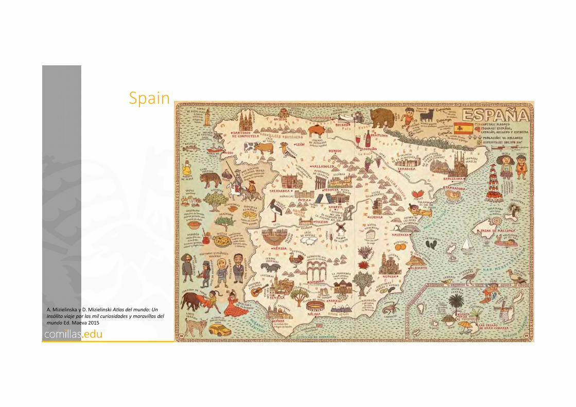
Spain
A. Mizielinska y D. Mizielinski Atlas del mundo: Un
insólito viaje por las mil curiosidades y maravillas del
mundo Ed. Maeva 2015

4Electricity Markets and Power Systems Optimization. February 2018
Which is the most Spanish beautiful landscape?
Aigüestortes
National Park Beach of
Menorca
Mediterranean
oak woodGuadalquivir
marshland

5Electricity Markets and Power Systems Optimization. February 2018
Introductions to
1. Power Systems
2. Optimization
3. Electricity Markets
4. Decision Support Models

1
Power Systems(original material from Prof. Javier García)
1. Power Systems
2. Optimization
3. Electricity Markets
4. Decision Support Models

7Electricity Markets and Power Systems Optimization. February 2018
8Electricity Markets and Power Systems Optimization. February 2018
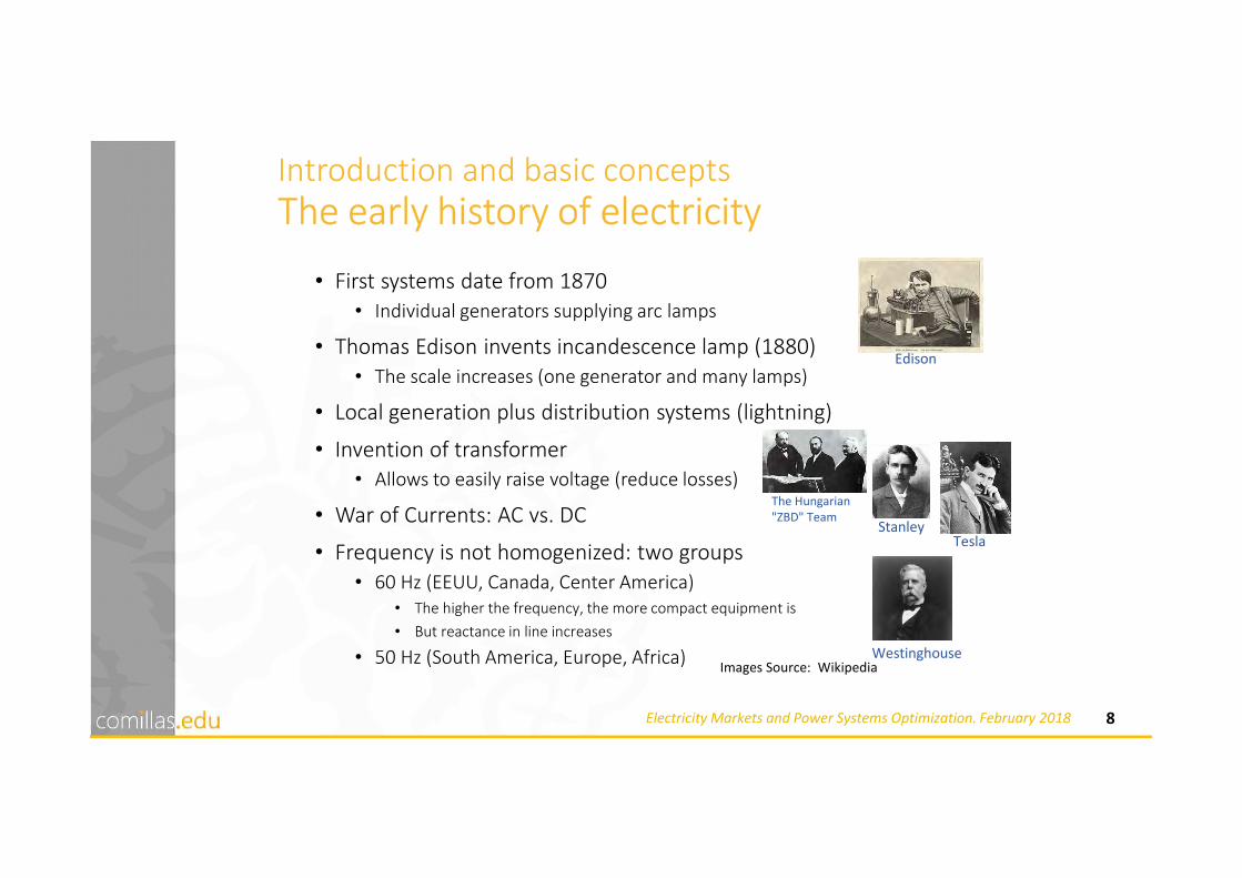
Introduction and basic conceptsThe early history of electricity
• First systems date from 1870• Individual generators supplying arc lamps
• Thomas Edison invents incandescence lamp (1880)• The scale increases (one generator and many lamps)
• Local generation plus distribution systems (lightning)
• Invention of transformer• Allows to easily raise voltage (reduce losses)
• War of Currents: AC vs. DC
• Frequency is not homogenized: two groups• 60 Hz (EEUU, Canada, Center America)
• The higher the frequency, the more compact equipment is
• But reactance in line increases
• 50 Hz (South America, Europe, Africa)
Edison
The Hungarian
"ZBD" Team Stanley
Tesla
WestinghouseImages Source: Wikipedia

10Electricity Markets and Power Systems Optimization. February 2018
Introduction and basic concepts
Evolution of production
Source: http://www.eia.gov/
Standardization of electricity led to a constant increase in consumption

11Electricity Markets and Power Systems Optimization. February 2018
Introduction and basic conceptsThe importance of power systems
• Secondary energy source• Transformed from primary energy sources
• It is a versatile and clean (at the consumption place)
• Highly correlated with the GDP
Electricity
Population
GDP
Primary sources

12Electricity Markets and Power Systems Optimization. February 2018
Introduction and basic conceptsThe importance of power systems
• Yearly variation of % electricity growth and GDP in developed countries
Source: EIA

13Electricity Markets and Power Systems Optimization. February 2018
Introduction and basic conceptsThe importance of power systems
• Relationship between GDP and electricity consumption worldwide (per capita terms)
Source: Energía y sociedad

14Electricity Markets and Power Systems Optimization. February 2018
Introduction and basic conceptsElectricity in the global energy system
1 Mtoe – 11.6 TWh
50 – wind/solar/tide (*)
Biofuels
(*) In 2013, wind/solar/tide accounted for 95 Mtoe (IEA)

15Electricity Markets and Power Systems Optimization. February 2018
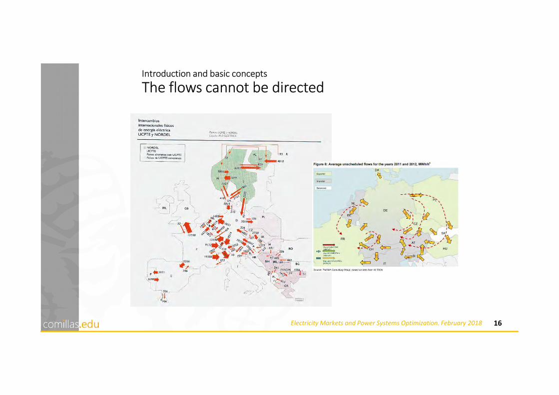
Introduction and basic conceptsBasic characteristics of electricity
It cannot be stored
It is injected and extracted in the different nodes, but the flow cannot be
directed
The electricity system is a dynamic system which has to ensure the
generation-demand balance
• Consumption is produced (transported) in real time
• It follows Kirchhoff laws (not commercial transactions between two parties)
• From the moment a line is congested, the cheaper generation cannot
always be dispatched
• Failure of one element introduces perturbations
• Rapidly spread: reserves needed
16Electricity Markets and Power Systems Optimization. February 2018
Introduction and basic concepts
The flows cannot be directed

17Electricity Markets and Power Systems Optimization. February 2018
Introduction and basic conceptsBasic characteristics of electricity• Control center REE (CECOEL y CECORE)
• Control center REE (CECRE) Continuous monitoring is needed
Powerful computers run models
• Estimate demand
• Simulate the generation
• Network flows
• Contingencies

18Electricity Markets and Power Systems Optimization. February 2018
Introduction and basic conceptsStructure and activities involved
Several available technologies
Investments (optimal mix)
Planning/Operation
Networks: Transmission /Distribution
Investments
Maintenance
Operation
Metering
Billing
Coordination by the System Operator:
Feasible production program
International interchanges
19Electricity Markets and Power Systems Optimization. February 2018
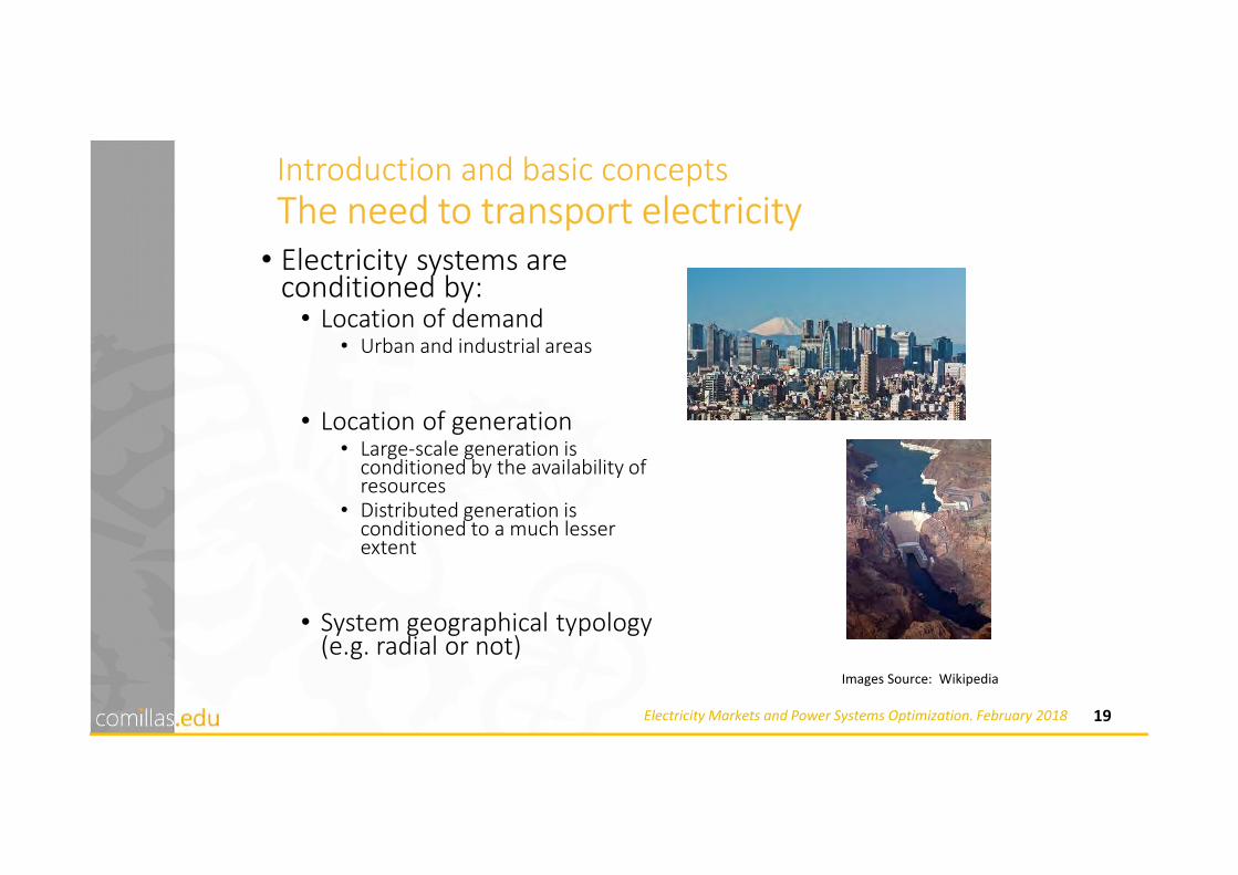
Introduction and basic conceptsThe need to transport electricity
• Electricity systems are conditioned by:
• Location of demand• Urban and industrial areas
• Location of generation• Large-scale generation is
conditioned by the availability of resources
• Distributed generation is conditioned to a much lesser extent
• System geographical typology (e.g. radial or not)
Images Source: Wikipedia

20Electricity Markets and Power Systems Optimization. February 2018
Description of power systems

21Electricity Markets and Power Systems Optimization. February 2018

22Electricity Markets and Power Systems Optimization. February 2018

23Electricity Markets and Power Systems Optimization. February 2018

24Electricity Markets and Power Systems Optimization. February 2018
• EU-27• 4,3 Mkm2,
• 493 Mhab,
• 11597 b€ GDP
• 741 GW installed capacity
• 3309 TWh/year
(Installed capacity, annual production)
• Germany ( 194 GW, 651 TWh)
• France ( 129 GW, 546 TWh)
• UK ( 81 GW, 336 TWh)
• Italy ( 121 GW, 269 TWh)
• Spain (108 GW, 248 TWh)
• USA• 9,8 Mkm2,
• 300 Mhab,
• 13195 b$ GDP
• 1076 GW installed capacity
• 4200 TWh/year
• PJM ( 183 GW, 837 GWh)
• ERCOT ( 80 GW, 347 TWh)
• California ( 79 GW, 195 TWh)
• NY-ISO ( 39 GW, 142 TWh)
• NE-ISO ( 31 GW, 136 TWh)
Introduction and basic concepts
A global perspective

25Electricity Markets and Power Systems Optimization. February 2018
Transforming “input” into “output”
coal
gas
hydro inflows
wind
uranium
electricity
others...

30Electricity Markets and Power Systems Optimization. February 2018
Electricity as a commodity
• Electricity is considered a commodity, “a marketable item produced to satisfy wants or needs”.
• The term commodity is used to describe a class of goods for which there is demand, but which is supplied without qualitative differentiation across a market.
• Its price is determined as a function of its market as a whole.
• Storing electricity in big quantities is uneconomical (at present). This makes this commodity a special one:
Electricity must be produced as soon as it is consumedElectricity must be produced as soon as it is consumed

1.1
Power generation(original material from Prof. Javier García)

33Electricity Markets and Power Systems Optimization. February 2018
Generation units: Coal-fired
source: © Tennessee Valley Authority
• Thermal generators are subject to many operational constraints due to their technical complexity:
• The coal is pulverized in the mills,
mixed with hot primary air and conducted
to the burner wind-box.
• The quantity of coal entering the mills is
a control variable.
• Steam production in the burner.
• Combustion stability problems
results in the existence of a
minimum output power.
• The water level in drum & the
superheated steam temperature
are control variables.
water is first evaporated to
steam, which is then
superheated, expanded
through a turbine and then
condensed back to water
Source: Wikipedia
34Electricity Markets and Power Systems Optimization. February 2018
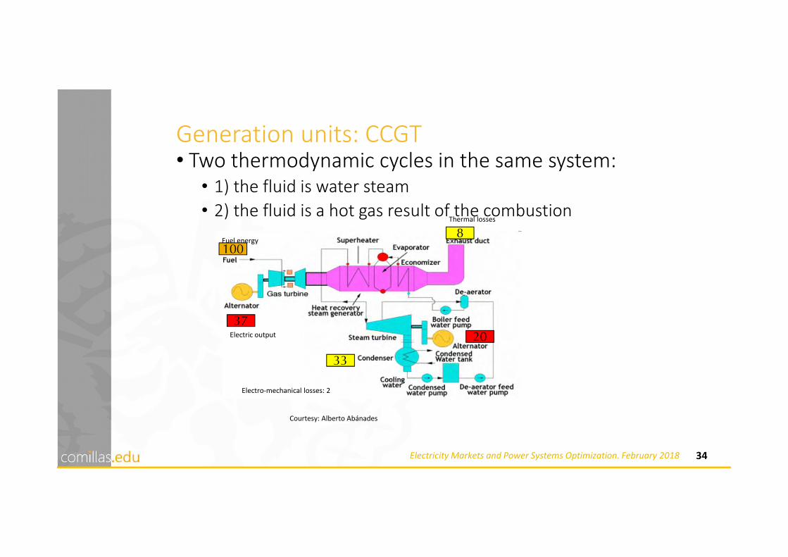
Generation units: CCGT• Two thermodynamic cycles in the same system:
• 1) the fluid is water steam
• 2) the fluid is a hot gas result of the combustion
Courtesy: Alberto Abánades
100
37
20
8
33
Electro-mechanical losses: 2
Fuel energy
Electric output
Thermal losses

36Electricity Markets and Power Systems Optimization. February 2018
Generation units: Nuclear generation
https://www.nuclear-power.net/nuclear-power-plant/

37Electricity Markets and Power Systems Optimization. February 2018
Comparison among thermal unitsEfficiency
[%]
Heat rate
[MBtu/MWh]
Capital cost
[€/kW]
Construction
time
[months]
Land use
[m2]
CO2
[kg/kWh]
CCGT plant 49 – 58 6.8-7.5 450 26 – 29 (400 MW) 30.000 ≤ 0.45
Coal-fired
plant
37 – 45 10-15 850 40 (1000 MW)
100.000
≥ 0.85 -1
Nuclear plant 34 10-15 1.500 60 (1000 MW)
70.000
---
Load change Warm start-up to
full load
Cold start-up to
full power
CCGT plant 10% / minute 40 minutes 2 hours
Coal-fired plant 4% / minute 3 hours 7 hours
Operation:

38Electricity Markets and Power Systems Optimization. February 2018
Scheme of a hydro plant

39Electricity Markets and Power Systems Optimization. February 2018
Generation units: Hydro generation• Hydroelectric systems are commonly divided into a set of
un-coupled basins
Inflow location
River basin 1
River basin 2
River basin 3Reservoir plant
Run-of-river plant

40Electricity Markets and Power Systems Optimization. February 2018
Hydro generation characteristics
Transfer flows
Overlaps
Guideline curves
Delay time
Water rights
Static data
Inter-temporal and spatial links
Non linear dependence among the water flow, the net head and the output power
Different and conflicting uses of the water
2030
4050
6070
80
15
20
25
30
35
40
45
0
10
20
30
40
50
60
[MW]p
3 [m /s]q 3 [Hm ]v

42Electricity Markets and Power Systems Optimization. February 2018
Pumped-storage hydro unit
Bombeo [MW]
rendimiento ηTurbinación [MW]
Volumen del Embalse Superior [MMh]
Volumen del Embalse Inferior [MMh]
• In isolated facilities, the pumpingcycle is daily or weekly
• The efficiency of the whole process is approx. 70%
• Normally, there are discrete functioningpoints when pumping.
Source: Wikipedia

43Electricity Markets and Power Systems Optimization. February 2018
Renewable energy sources
• Wind power: onshore and offshore
• Solar: photovoltaics (PV) and concentrated solar power (CSP)
• Biomass
• Biofuel
• Geothermal energy
• Small hydropower

44Electricity Markets and Power Systems Optimization. February 2018
• How can it be possible to meet the demand at any time efficiently and reliably, for an infinite time horizon and under uncertainty?
• The answer: Use a temporal hierarchy of decisions• Decision functions hierarchically chained
• Each function optimizes its own decisions
subject to• Its own constraints
• Constraints that are imposed from upper levels
Question:
Which are the main operation
decisions to be made?

1.2
Hierarchy of models(original material from Prof. Javier García)

46Electricity Markets and Power Systems Optimization. February 2018
• Real time operation
• Operation
• Operation planning
• Expansion planning
Time scales

47Electricity Markets and Power Systems Optimization. February 2018
What decisions to take?
• Active and reactive power of the committed generators
• Load shedding• Flow control of lines equipped with power
electronics (FACTS and DC links)• Phase shifter angles• Transformer tap position• Operating reserves• Local control parameters• Configuration of the network• Commitment of the generators• Hydro reservoir operation• Maintenance schedules• Introduction and retirement of generation
facilities• Network expansion

48Electricity Markets and Power Systems Optimization. February 2018
Not under control
• Load• Equipment failure• Faults• Output of variable energy resources (but can curtail)• Power flows in most lines (need to respect circuit Kirchhoff’
laws)• Fuel consumption of thermal units for a given output
49Electricity Markets and Power Systems Optimization. February 2018
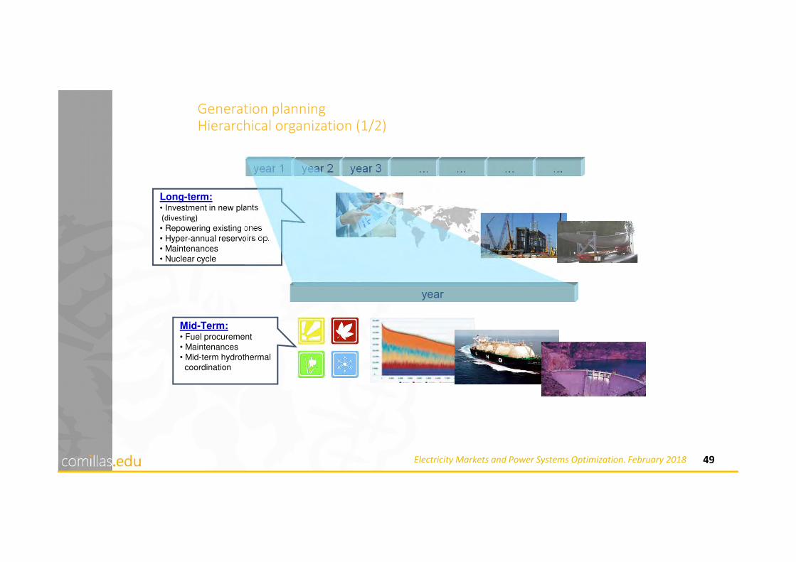
Generation planningHierarchical organization (1/2)
year 1 year 2 year 3 … … … …
Long-term:• Investment in new plants(divesting)
• Repowering existing ones
• Hyper-annual reservoirs op.
• Maintenances
• Nuclear cycle
Mid-Term:• Fuel procurement
• Maintenances
• Mid-term hydrothermal
coordination
year

50Electricity Markets and Power Systems Optimization. February 2018
0
2 0 0 0
4 0 0 0
6 0 0 0
8 0 0 0
1 0 0 0 0
1 2 0 0 0
1 7
13
19
25
31
37
43
49
55
61
67
73
79
85
91
97
103
109
115
121
127
133
139
145
151
157
163
N U L P L N C I H N F U
G S G F H ID R O T B B B D R
Generation planningHierarchical organization (2/2)
year
Sat Sun Mon Tue Wed Thu Fri
Real time
• Real time operation: AGC
(Automatic Generation Control)
week
START-UP SHUT-DOWN
1 2 3 4 5 6 7 8 9 10 11 12 13 14 15 16 17 18 19 20 21 22 23 24G1 1000 1000 1000 1000 1000 1000 1000 1000 1000 1000 1000 1000 1000 1000 1000 1000 1000 1000 1000 1000 1000 1000 1000 1000G2 700 700 700 700 700 700 700 700 700 700 700 700 700 700 700 700 700 700 700 700 700 700 700 700G3 500 383 463 500 500 461 383 500 500 500 500 500 500 500 500 500 500 500 500 500 500 500 500 500G4 350 297 243 215 215 243 297 350 350 350 350 350 350 350 350 350 350 350 350 350 350 350 350 350G5 350 297 243 243 297 243 297 350 350 350 350 350 350 350 350 350 350 350 350 350 350 350 350 350G6 350 297 243 297 243 243 297 350 350 350 350 350 350 350 350 350 350 350 350 350 350 350 350 350
G7 350 297 243 297 297 243 297 350 350 306 350 350 350 350 350 350 350 350 350 350 350 350 350 350
G8 393 277 160 160 160 277 393 510 510 393 510 510 510 510 510 510 510 510 510 510 510 510 510 510G9 510 393 277 160 160 160 277 393 510 393 510 510 510 510 510 510 510 510 510 510 510 510 510 510G10 217 175 175 175 175 175 175 217 258 258 300 300 300 300 300 300 300 300 300 281 300 300 300 258G11 0 0 0 0 0 0 0 0 209 271 333 340 340 340 340 340 340 340 340 278 217 163 225 217G12 0 0 0 0 0 0 0 0 217 278 340 340 340 340 340 340 340 340 340 278 217 267 217 155G13 0 0 0 0 0 0 0 0 0 180 240 300 300 300 300 300 300 300 300 240 180 120 120 120G14 0 0 0 0 0 0 0 0 0 0 203 262 320 320 320 320 320 320 262 203 145 145 145 145G15 0 0 0 0 0 0 0 0 0 0 203 262 320 320 320 320 320 320 278 220 162 145 145 145G16 0 0 0 0 0 0 0 0 0 0 220 275 175 175 175 175 175 175 275 165 110 110 110 110G17 0 0 0 0 0 0 0 0 0 0 0 0 0 0 0 0 0 0 0 0 0 0 0 0G18 0 0 0 0 0 0 0 0 0 0 0 0 0 0 0 0 0 0 0 0 0 0 0 0G19 0 0 0 0 0 0 0 0 0 0 127 77 60 60 60 60 60 60 60 60 60 60 60 60G20 0 0 0 0 0 0 0 0 0 0 0 0 0 0 0 0 0 0 0 0 0 0 0 0G21 0 0 0 0 0 0 0 0 0 0 0 0 0 0 0 0 0 0 0 0 0 0 0 0G22 0 0 0 0 0 0 0 0 0 0 0 0 0 0 0 0 0 0 0 0 0 0 0 0
CH1 50 50 50 50 50 50 50 50 50 50 50 50 50 50 50 50 50 50 50 50 50 50 50 50CH2 350 35 35 35 35 35 35 350 35 35 350 350 350 350 350 350 350 350 350 35 35 35 35 125
UBT1 88 0 0 0 0 0 0 103 0 0 120 120 120 120 38 86 120 120 120 0 0 0 0 0UBT2 0 0 0 0 0 0 0 0 0 0 80 80 80 80 0 0 80 80 80 0 0 0 0 0
UBT1 0 100 100 100 100 100 100 0 100 100 0 0 0 0 0 0 0 0 0 100 76 0 0 0UBT2 0 60 60 60 60 60 60 0 42 60 0 0 0 0 0 0 0 0 0 60 0 0 0 0
Hourly:• Economic Dispatch
• Optimal Power Flow (OPF)
Daily:• UC for reaching the peak load
• Hourly scheduling
Weekly:• Unit-Commitment (UC)
Start-up (Monday)
Shut-down (weekend)
• Hydrothermal coordination
• Hourly scheduling

2
Optimization
1. Power Systems
2. Optimization
3. Electricity Markets
4. Decision Support Models

54Electricity Markets and Power Systems Optimization. February 2018
• Descriptive: statistics (data analysis, analysis of variance, correlation)
• Predictive: simulation, regression, forecasting
• Prescriptive: optimization, heuristics, decision analysis
Business Analytics Spectrum
Stochastic Optimization How can we achieve the best outcome including the
effects of variability?
PRESCRIPTIVE
Optimization How can we achieve the best outcome?
Predictive modeling What will happen next if? PREDICTIVE
Forecasting What if these trends continue?
Simulation What could happen…?
Alerts What actions are needed?
Query/drill down What exactly is the problem? DESCRIPTIVE
Ad hoc reporting How many, how often, where?
Standard reporting What happened?
Co
mp
eti
tiv
e a
dv
an
tag
e
Source: A. Fleischer et al. ILOG Optimization for Collateral Management

55Electricity Markets and Power Systems Optimization. February 2018
Example: Operation Planning
Glassware S.A. manufactures products of glass of high quality, including windows and doors. It has three factories. Factory 1 manufactures aluminum frames and metal parts. Factory 2 manufactures wooden frames and factory 3 manufactures glass and assembles the products.
Due to revenue losses, the directorship has decided to change the product line. Unprofitable ones are going to be discontinued and two new ones with high selling potential are to be launched:
• Product no. 1: glass door with aluminum frame
• Product no. 2: glass window with wooden frame
The first product requires to be processed in factories 1 and 3, while the second one needs 2 and 3. The Marketing Department estimates that as many doors and windows as can be manufactured can be sold. But given that both products compete by the factory 3 resources, we want to know the product mix that maximizes the company profits.

56Electricity Markets and Power Systems Optimization. February 2018
Example: Operation Planning
1 2
1
2
1 2
1 2
max z 3 5
4
2 12
3 2 18
, 0
x x
x
x
x x
x x
= +≤≤
+ ≤≥
PI
SX
(4,0)
(4,3)
(2,6)
(0,6)
(0,0)
x2
x1
Lines of equal objective function

57Electricity Markets and Power Systems Optimization. February 2018
My first minimalist optimization modelpositive variables x1, x2
variable z
equations of, e1, e2, e3 ;
of .. 3*x1 + 5*x2 =e= z ;e1 .. x1 =l= 4 ;e2 .. 2*x2 =l= 12 ;e3 .. 3*x1 + 2*x2 =l= 18 ;
model minimalist / all /solve minimalist maximizing z using LP
max��,�� � 3�� 5���� � 42�� � 12
3�� 2�� � 18��, �� � 0

58Electricity Markets and Power Systems Optimization. February 2018
Transportation modelThere are � can factories and � consumption markets. Each factory has a maximum capacity of �� cases and each market demands a quantity of �� cases (it is assumed that the total production capacity is greater than the total market demand for the problem to be feasible). The transportation cost between each factory � and each market � for each case is ���. The demand must be satisfied at minimum cost.The decision variables of the problem will be cases transported between each factory � and each market j, ���.

59Electricity Markets and Power Systems Optimization. February 2018
Mathematical formulation
• Objective function
min��� �!"�!"#
!"• Production limit for each factory �
�!"#
"� �! ∀�
• Consumption in each market � �!"#
!� �" ∀�
• Quantity to send from each factory � to each market ��!" � 0∀� → �
60Electricity Markets and Power Systems Optimization. February 2018
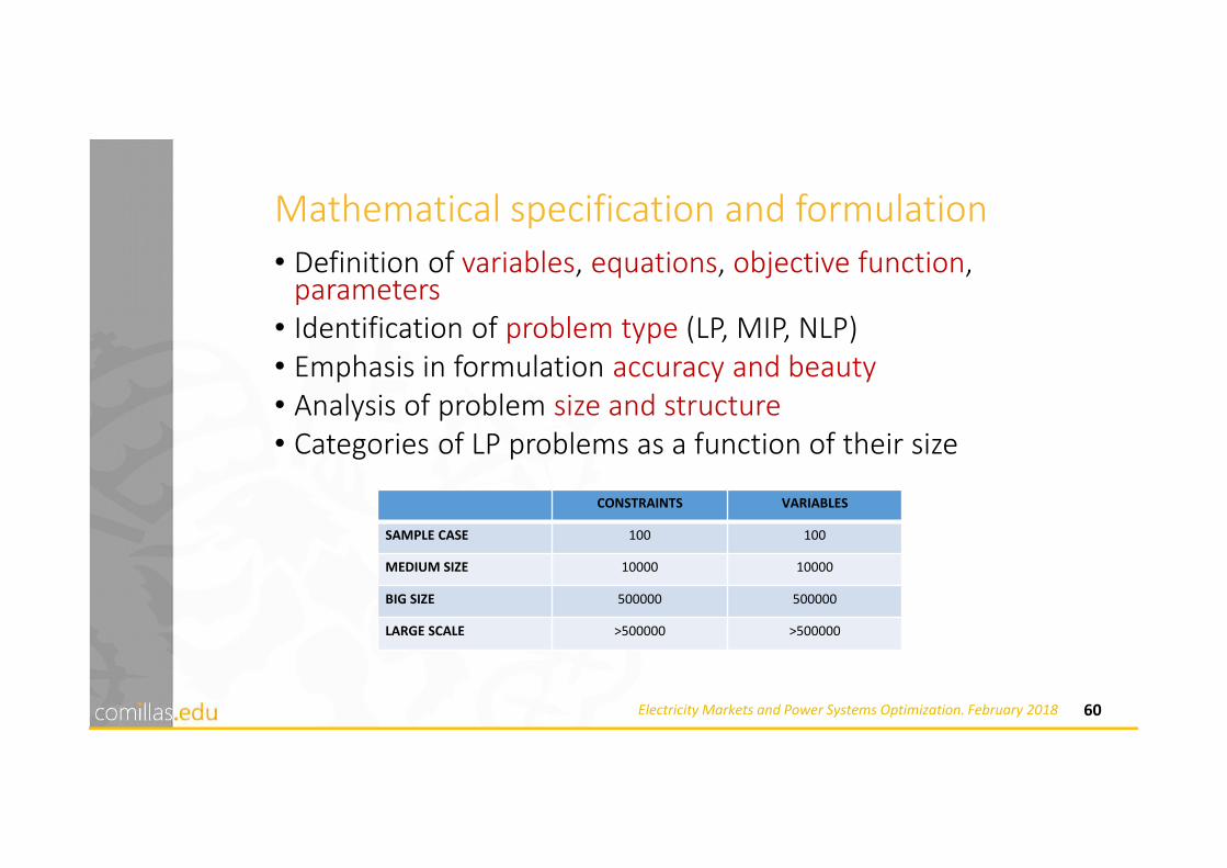
Mathematical specification and formulation• Definition of variables, equations, objective function,
parameters• Identification of problem type (LP, MIP, NLP)• Emphasis in formulation accuracy and beauty• Analysis of problem size and structure• Categories of LP problems as a function of their size
CONSTRAINTS VARIABLES
SAMPLE CASE 100 100
MEDIUM SIZE 10000 10000
BIG SIZE 500000 500000
LARGE SCALE >500000 >500000

61Electricity Markets and Power Systems Optimization. February 2018
Algebraic modeling languages advantages (i)
• High level languages for compact formulation of large-scale and complex models
• Easy prototype development• Documentation is made simultaneously to modeling• Improve modelers productivity• Structure good modeling habits• Easy continuous reformulation• Allow to build large maintainable models that can be adapted
quickly to new situations

62Electricity Markets and Power Systems Optimization. February 2018
Algebraic modeling languages advantages (ii)
• Separation of interface, data, model and solver
• Formulation independent of model size
• Model independent of solvers
• Allow advanced algorithm implementation
• Easy implementation of NLP, MIP, and MCP
• Open architecture with interfaces to other systems
• Platform independence and portability among platforms and operating systems (MS Windows, Linux, Mac OS X, Sun Solaris, IBM AIX)

63Electricity Markets and Power Systems Optimization. February 2018
Search, compare and if you find something better use it
v. 25.0.2
v. 0.6.2
v. 5.2

64Electricity Markets and Power Systems Optimization. February 2018
Interfaces, languages, solvers
Mathematical Language Algebraic Language
GAMS
AMPL
AIMMS
Python Pyomo
Julia JuMP
MatLab
Solver Studio
Solver
IBM CPLEX
Gurobi
XPRESS
GLPK
CBC
PATH
Interface
(graphical)
Excel
Access
SQL
Matlab

65Electricity Markets and Power Systems Optimization. February 2018
• GAMS Model Librarieshttps://www.gams.com/latest/gamslib_ml/libhtml/index.html#gamslib
• Decision Support Models in the Electric Power Industry https://www.iit.comillas.edu/aramos/Ramos_CV.htm#ModelosAyudaDecision
Learning by reading first, and then by doing

66Electricity Markets and Power Systems Optimization. February 2018
GAMS (General Algebraic Modeling System)
GAMS birth: 1976 World Bank slide

67Electricity Markets and Power Systems Optimization. February 2018
Developing in GAMS
• Development environment gamside
• Documentation• GAMS Documentation Center https://www.gams.com/latest/docs/
• GAMS Support Wiki https://support.gams.com/
• Bruce McCarl's GAMS Newsletter https://www.gams.com/community/newsletters-mailing-list/
• Users guide Help > GAMS Users Guide
• Solvers guide Help > Expanded GAMS Guide
• Model: FileName.gms
• Results: FileName.lst
• Process log: FileName.log
aaa.gpr
68Electricity Markets and Power Systems Optimization. February 2018
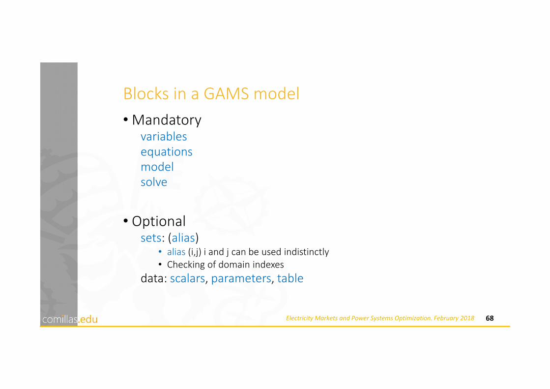
Blocks in a GAMS model
• Mandatoryvariablesequationsmodelsolve
• Optionalsets: (alias)
• alias (i,j) i and j can be used indistinctly• Checking of domain indexes
data: scalars, parameters, table

69Electricity Markets and Power Systems Optimization. February 2018
min��� �!"�!"#
!"
�!"#
"� �! ∀�
�!"#
!� �"∀��!" � 0
My first transportation model (classical organization)sets
I origins / VIGO, ALGECIRAS / J destinations / MADRID, BARCELONA, VALENCIA /
parameters pA(i) origin capacity / VIGO 350 ALGECIRAS 700 /
pB(j) destination demand / MADRID 400 BARCELONA 450 VALENCIA 150 /
table pC(i,j) per unit transportation cost MADRID BARCELONA VALENCIAVIGO 0.06 0.12 0.09ALGECIRAS 0.05 0.15 0.11
variables vX(i,j) units transported vCost transportation cost
positive variable vX
equations eCost transportation cost eCapacity(i) maximum capacity of each origin eDemand (j) demand supply at destination ;
eCost .. sum[(i,j), pC(i,j) * vX(i,j)] =e= vCost ;eCapacity(i) .. sum[ j , vX(i,j)] =l= pA(i) ;eDemand (j) .. sum[ i , vX(i,j)] =g= pB(j) ;
model mTransport / all /solve mTransport using LP minimizing vCost
A. Mizielinska y D. Mizielinski Atlas del mundo: Un insólito viaje por las
mil curiosidades y maravillas del mundo Ed. Maeva 2015

70Electricity Markets and Power Systems Optimization. February 2018
Unit commitment and economic dispatch• S. Cerisola, A. Baillo, J.M. Fernandez-Lopez, A. Ramos, R. Gollmer Stochastic Power Generation Unit
Commitment in Electricity Markets: A Novel Formulation and A Comparison of Solution MethodsOperations Research 57 (1): 32-46 Jan-Feb 2009 (http://or.journal.informs.org/cgi/content/abstract/57/1/32)

71Electricity Markets and Power Systems Optimization. February 2018
Smart Charging of Electric Vehicles
• P. Sánchez, G. Sánchez González Direct Load Control Decision Model for Aggregated EV charging points IEEE Transactions on Power Systems vol. 27 (3): 1577-1584 August 2012

72Electricity Markets and Power Systems Optimization. February 2018
Off-shore wind farm electric design• S. Lumbreras and A. Ramos Optimal Design of the Electrical Layout of an Offshore Wind Farm: a
Comprehensive and Efficient Approach Applying Decomposition Strategies IEEE Transactions on Power Systems 28 (2): 1434-1441, May 2013 10.1109/TPWRS.2012.2204906
• S. Lumbreras and A. Ramos Offshore Wind Farm Electrical Design: A Review Wind Energy 16 (3): 459-473 April 2013 10.1002/we.1498
• M. Banzo and A. Ramos Stochastic Optimization Model for Electric Power System Planning of Offshore Wind Farms IEEE Transactions on Power Systems 26 (3): 1338-1348 Aug 2011 10.1109/TPWRS.2010.2075944

73Electricity Markets and Power Systems Optimization. February 2018
Generation Capacity Expansion Problem• S. Wogrin, E. Centeno, J. Barquín Generation capacity expansion analysis: Open loop approximation
of closed loop equilibria IEEE Transactions on Power Systems vol. 28, no. 3, pp. 3362-3371, August 2013.

3
Electricity Markets
1. Power Systems
2. Optimization
3. Electricity Markets
4. Decision Support Models
75Electricity Markets and Power Systems Optimization. February 2018
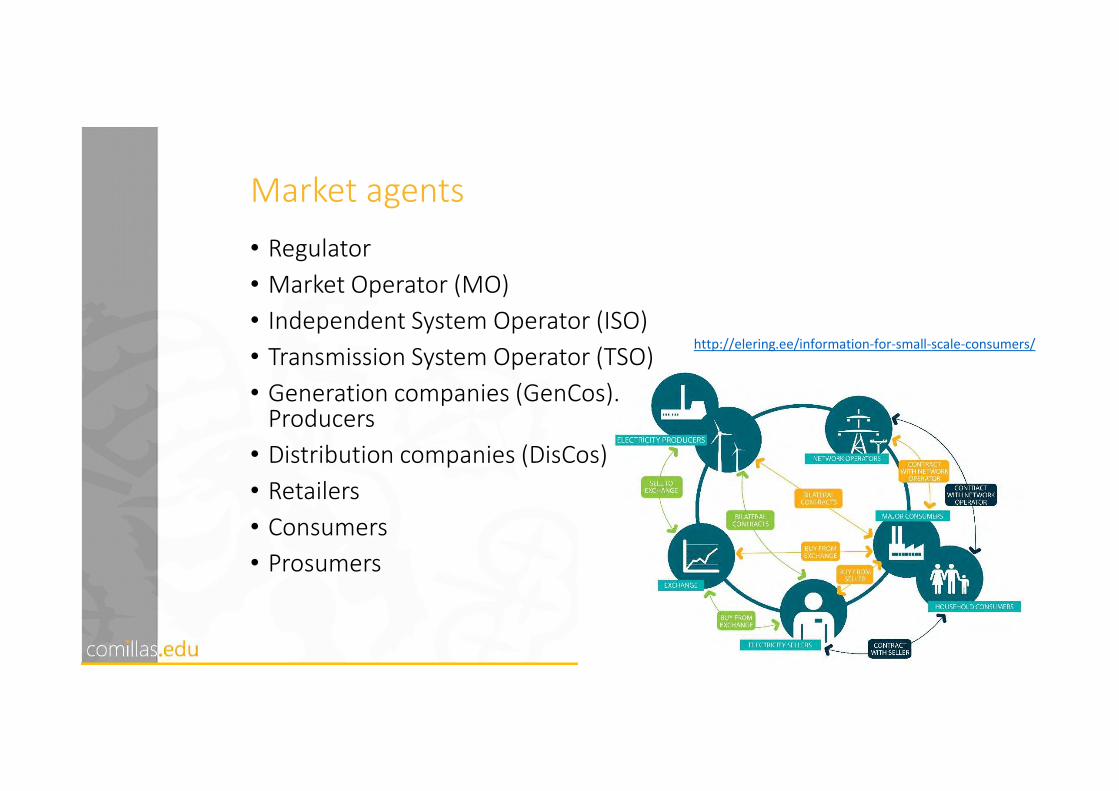
Market agents
• Regulator
• Market Operator (MO)
• Independent System Operator (ISO)
• Transmission System Operator (TSO)
• Generation companies (GenCos). Producers
• Distribution companies (DisCos)
• Retailers
• Consumers
• Prosumers
http://elering.ee/information-for-small-scale-consumers/

76Electricity Markets and Power Systems Optimization. February 2018
Electric System. Activities, businesses and markets
Source: Iberdrola

77Electricity Markets and Power Systems Optimization. February 2018
Wholesale Markets

78Electricity Markets and Power Systems Optimization. February 2018
Spanish electricity market• Starts January 1st, 1998
• Sequence of (energy and power) markets.• Day-ahead market• Adjustment services
• Technical constraints
• Intra-day market• Reserve market
• Secondary reserve• Tertiary reserve
• Imbalance management
SupplyImbalance management
Reserve
market
Intra-day markets
Technical constraints
Day-
market
Day-ahead market

79Electricity Markets and Power Systems Optimization. February 2018
Day-Ahead Market
Technical constraints management (DM)
Secondary regulation capacity
Intra-Day Market:
Sessions 1 a 6 Technical constraints management (IM)
Generation-load imbalance mechanism
Tertiary reserve
Technical constraints management (RT)
Market Operator
< 11.00 h
14.00 h
16.00 h
18.30 h…
19.20 h
21.00 h…
15 min before
Real Time
System Operator: Red Eléctrica de España
Previous information < 9.00 h
Nomination schedules < 12.00 h
Source: M. de la Torre, J. Paradinas Integration of renewable generation. The case of Spain
Sequence of markets

80Electricity Markets and Power Systems Optimization. February 2018
MIBEL. Daily market. Aggregate supply and demand curves
1 hour
81Electricity Markets and Power Systems Optimization. February 2018
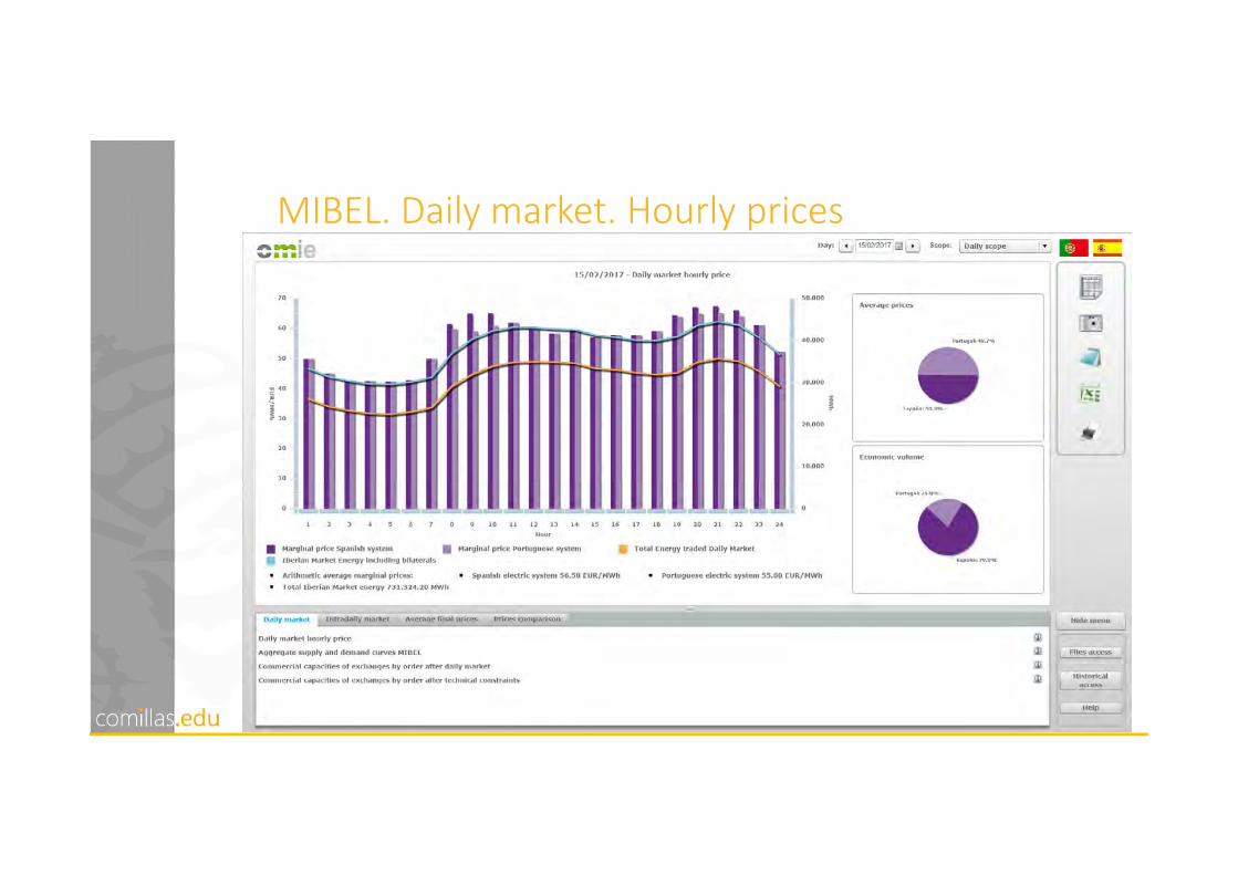
MIBEL. Daily market. Hourly prices

82Electricity Markets and Power Systems Optimization. February 2018
MIBEL. 1st Intra-day market. Aggregate supply and demand curves
1 hour

83Electricity Markets and Power Systems Optimization. February 2018
MIBEL. 1st Intra-day market. Hourly prices

84Electricity Markets and Power Systems Optimization. February 2018
Regional wholesale electricity markets
• Central Western Europe (Austria, Belgium, France, Germany, the Netherlands, Switzerland)
• British Isles (UK, Ireland)
• Northern Europe (Denmark, Estonia, Finland, Latvia, Lithuania, Norway, Sweden)
• Apennine Peninsula (Italy)
• Iberian Peninsula (Spain and Portugal)
• Central Eastern Europe (Czech Republic, Hungary, Poland, Romania, Slovakia, Slovenia)
• South Eastern Europe (Greece and Bulgaria)

85Electricity Markets and Power Systems Optimization. February 2018
Average wholesale baseloadelectricity prices. 2016 Q3
https://ec.europa.eu/energy/en/data-analysis/market-analysis

3.1
Market Equilibrium Model

88Electricity Markets and Power Systems Optimization. February 2018
Bibliography• M. Ventosa, A. Baíllo, A. Ramos, M. Rivier Electricity Market Modeling Trends
Energy Policy 33 (7): 897-913 May 2005
• M. Rivier, M. Ventosa, A. Ramos, F. Martínez-Córcoles, A. Chiarri “A GenerationOperation Planning Model in Deregulated Electricity Markets based on theComplementarity Problem” in the book M.C. Ferris, O.L. Mangasarian and J-S. Pang(eds.) Complementarity: Applications, Algorithms and Extensions pp. 273-295Kluwer Academic Publishers 2001 ISBN 0792368169
• J. Bushnell (1998) “Water and Power: Hydroelectric Resources in the Era ofCompetition in the Western US”
(http://www.ucei.berkeley.edu/PDF/pwp056.pdf)
• J. Barquín, E. Centeno, J. Reneses, “Medium-term generation programming incompetitive environments: A new optimization approach for market equilibriumcomputing”, IEE Proceedings-Generation Transmission and Distribution. vol. 151,no. 1, pp. 119-126, January 2004.

89Electricity Markets and Power Systems Optimization. February 2018
Why a market equilibrium model?
• Electricity generation business
• Electricity production market
• Generating companies have new roles and responsibilities
• New decision-making tools and models that take into account the market
• Markets generally having only few companies
• Companies’ decisions are mutually dependent

90Electricity Markets and Power Systems Optimization. February 2018
Electricity market models
• Quantitative approach• Application of different statistical techniques using available
historical records
• Assumes that all the market results that can occur are contained in historical series
• Fundamental approach• Detailed representation of the system and considers input
variables:• Demand, fuel costs, hydro inflows, operation constraints, new
installed capacity, generator ownership
• Price is obtained as a result of the model
91Electricity Markets and Power Systems Optimization. February 2018
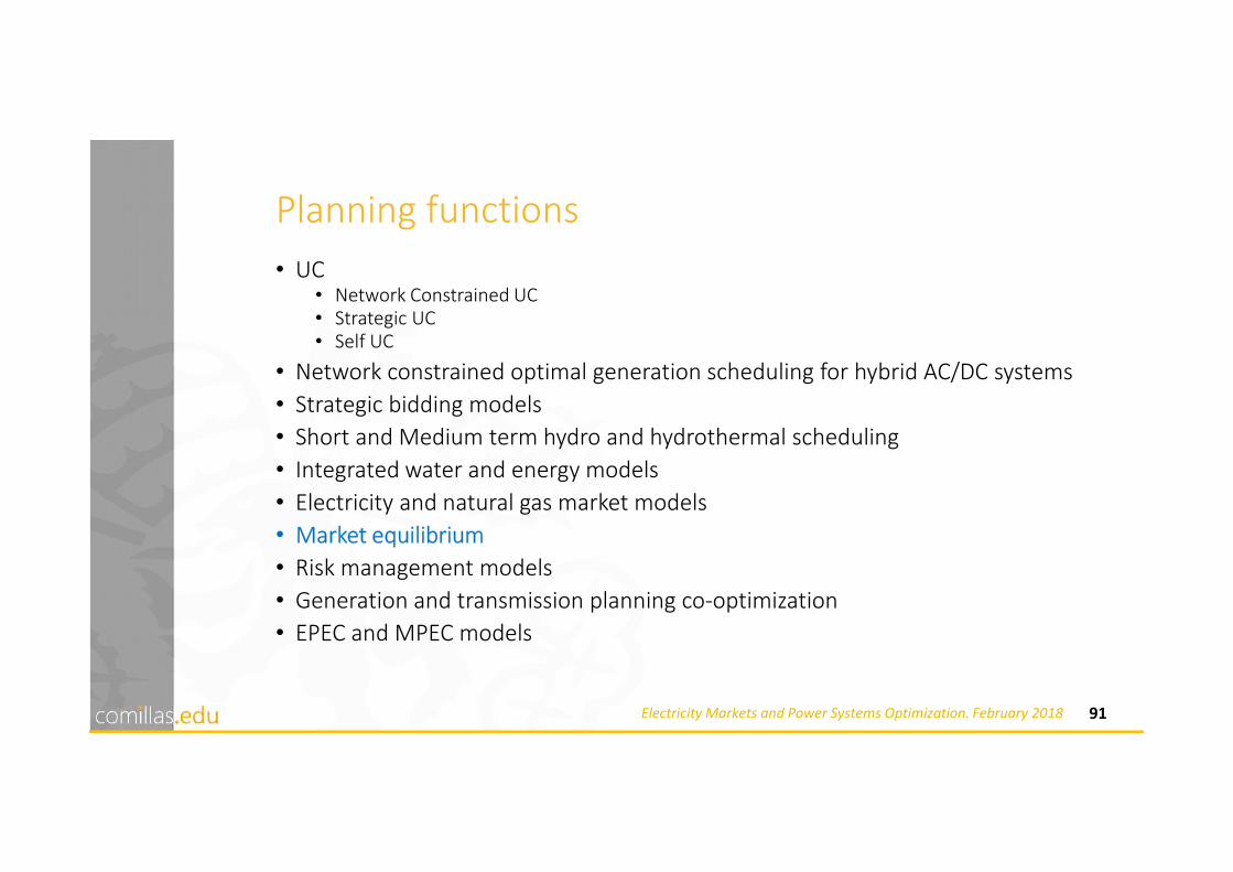
Planning functions
• UC• Network Constrained UC• Strategic UC• Self UC
• Network constrained optimal generation scheduling for hybrid AC/DC systems
• Strategic bidding models
• Short and Medium term hydro and hydrothermal scheduling
• Integrated water and energy models
• Electricity and natural gas market models
• Market equilibrium
• Risk management models
• Generation and transmission planning co-optimization
• EPEC and MPEC models

92Electricity Markets and Power Systems Optimization. February 2018
Fundamental models
Electricity market
models
(Fundamental)
Models covering all
generating companies
Models covering a
single generating
company
Equilibrium
models
Simulation
models
Price
Quantity
Supply functions
Price maker
Price taker
Parameterized
SFs
Multi part bids
Bid modeling

93Electricity Markets and Power Systems Optimization. February 2018
Scope
Regulated
system
“Cost-
based”
Liberalized
market
“Profit-
based”
Short TermMid TermLong Term
• Gas & coal supply management
• Mid-term hydrothermal coordination:
-Water value
• Capacity investment
• Maintenance
• Energy management- nuclear cycle
- hyper-annual reservoirs
• Unit-Commitment
• Short-term hydrothermal coordination
• Economic dispatch
• Strategic bidding:
- Energy
- Ancillary Services
• Objectives:
- Market share
- Price
• Budget estimation
• Bidding in derivatives markets
• Capacity investment (new & existing plants)
• Risk management
• Long-term contracts
- Fuel purchases
- Elect. derivatives
Models’ clasification

95Electricity Markets and Power Systems Optimization. February 2018
Why an equilibrium model based on the complementarity problem?
• Modeling the electricity market by a complementarity problem approach provides
• A flexible representation of the market and its medium- and long-term operation
• Modeling large-scale electricity schedules
• A technically feasible solution
• Actual, unique market equilibrium (in realistic conditions)
• Methods for solving complementarity problems (MCP)
• Allow realistic sizes: 10,000 variables
• Although solution time is greater than in linear optimization
• Alternative formulations and numerical solutions exist, based on the equivalent quadratic problem (QP)
• Same optimality conditions as the equilibrium problem
• Iterative solution of a linear problem
3.2
Cournot model – conjectural variations

98Electricity Markets and Power Systems Optimization. February 2018
Model based on the complementarity problem Means of production
• Fuel stock management
• Pumped storage hydro plants
Market aspects• Contracts for differences
• Take-or-pay contracts
Session outline
Bushnell model Hydro thermal generation
Multi-period
Cournot model Thermal generation
Single period

99Electricity Markets and Power Systems Optimization. February 2018
Cournot model (1838)
• Pioneer model to study companies’ strategic
behavior
• Simple model
• Single generating plant
• All the generating plants of each company are grouped
• Inter-period constraints not considered
• Single period equilibrium
• Assumes perfect information
• Applicable to medium- and long-term analyses of
thermal systems
French philosopher
and mathematician
(1801 –1877)

100Electricity Markets and Power Systems Optimization. February 2018
Cournot model: approach
• Main characteristics
• It explicitly considers
• Each company’s objective is to maximize profits
• Company decisions are interdependent
• Consumer behavior
• Nash equilibrium in quantity strategies: each firm chooses an output
quantity to maximize its profit. The Nash-Cournot market equilibrium
defines a set of outputs such that no firm, taking its competitors’ output
as given, wishes to change its own output unilaterally
• Price is derived from the inverse demand function
• These components are enough to interpret it as the origin of
more complex models, such as the model based on the
complementarity problem

101Electricity Markets and Power Systems Optimization. February 2018
Cournot model: formulation(https://www.iit.comillas.edu/aramos/StarMrkLite_CournotEn.gms)
• Objective function: profits
• Inverse demand function
• Cournot conjecture: vertical supply
• Optimality conditions
-e e eB p q C= ⋅
ee
p f q = ∑
* *( )
0e e e
e e e
q q qp pp
q q q q
∂ + ∂∂ ∂ ′= = ↔ =∂ ∂ ∂ ∂
e Company
e* Other companies
Be Profits
p Price
qe Output
Ce Variable costs
MCe Marginal cost
MRe Marginal revenue
p-MCe Price mark-up
( ) ( )0
ee
e e e e
e
e
e
p MCBMR p q p qMC q
q
q
p
∂
∂
−′= → = + = → =
′−
System of
equations
Own output decision will not
have an effect on the
decisions of the competitors
102Electricity Markets and Power Systems Optimization. February 2018
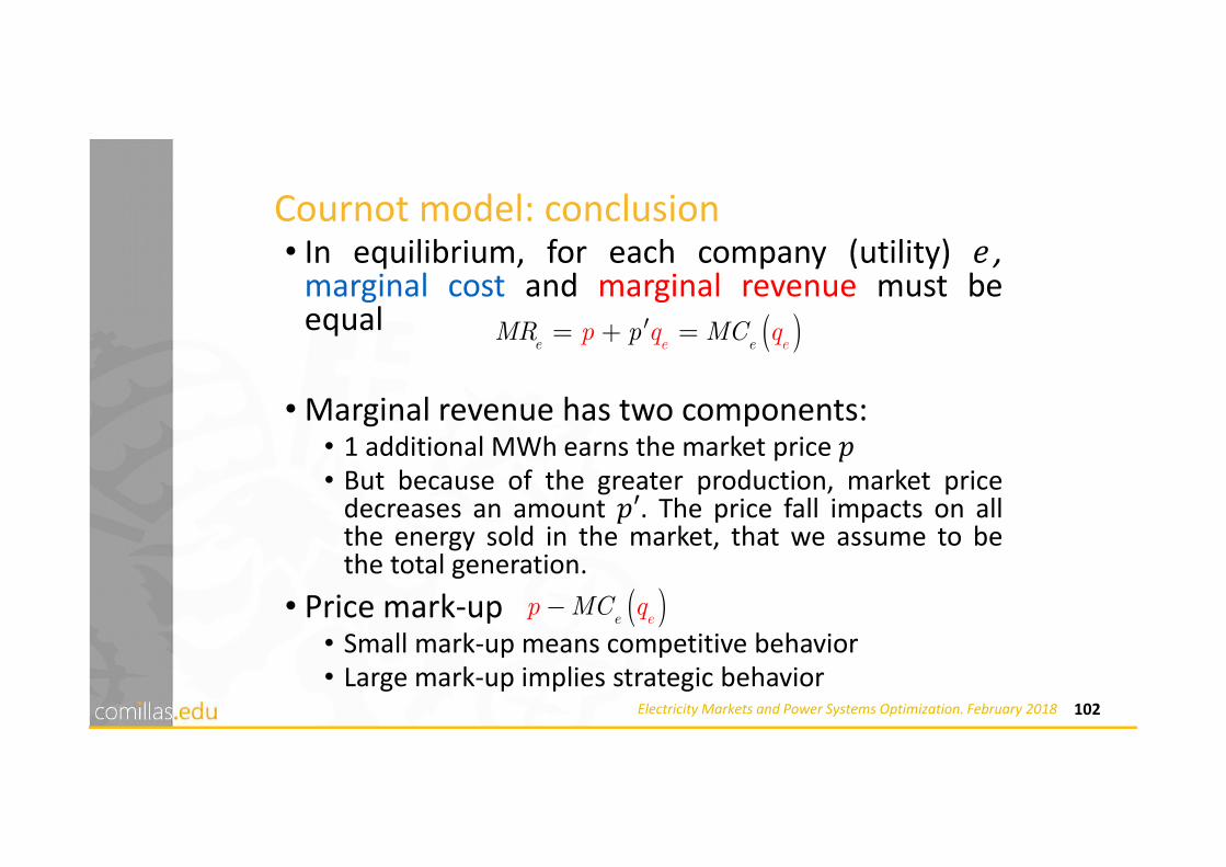
Cournot model: conclusion• In equilibrium, for each company (utility) ' ,
marginal cost and marginal revenue must beequal
• Marginal revenue has two components:• 1 additional MWh earns the market price (• But because of the greater production, market price
decreases an amount (′. The price fall impacts on allthe energy sold in the market, that we assume to bethe total generation.
• Price mark-up• Small mark-up means competitive behavior
• Large mark-up implies strategic behavior
( )e ee ep qMR p M qC′= + =
( )e ep MC q−

103Electricity Markets and Power Systems Optimization. February 2018
Cournot model with contracts
• Objective function
• Optimality conditions( )e e e e c e
B p q L C p L= − − +e Company
Be Profits
p Price
qe Output
Le Contracted output
pc Contract price
Ce Variable costs
MCe Marginal cost
MRe Marginal revenue( ) ( )( )
0e
e
e e e
e
e
e e
e
e
B
q
MR p q L p MC q
MCL
p
p qq
∂
∂=
′= + − =
−= +
′−

104Electricity Markets and Power Systems Optimization. February 2018
Cournot model: example (I)
• Perfect competition• Company 1: MC1 = 2 €/MW q1 MAX = 5 MW
• Company 2: MC2 = 3 €/MW q2 MAX = 5 MW
• Inverse demand function: p = 10 - (q1 + q2)
10
10
p
D = q1 + q2
5
2MC1 = 2 ; q1 MAX = 5
Inverse demand function
Competitive
supply function
MC2 = 3; q2 MAX = 53
Equilibrium under
perfect competition
7
€/MW
MW

105Electricity Markets and Power Systems Optimization. February 2018
Cournot model: example (II)
• Duopoly• Company 1: MC1 = 2 €/MW
• Company 2: MC2 = 3 €/MW
• IDF: p = 10 - (q1 + q2); p’=-1
10
10
p
D = q1 + q2
2
( )11
1
0 1 2B
p qq
∂
∂= → + ⋅ − =
( )22
2
0 1 3B
p qq
∂
∂= → + ⋅ − =
Cournot
q1 = 3
q2 = 23
7
p’=-1
5
5
Solving
q1 = 3, q2 = 2
p = 10 - (q1 + q2) = 5
€/MW
MW

106Electricity Markets and Power Systems Optimization. February 2018
From Cournot to conjectural variations (CV)
• Objective function
• Inverse demand function
• Conjecture: every company sees its residual demand
→ generalization of the model based on CV
• Optimality conditions
max -e e eB p q C= ⋅
e
e
pp
q
∂ ′=∂
( )0e e
e
e e
e
ep
BMR p M
qq C q
∂
∂′= → = + =
e Company
Be Profits
p Price
qe Output
Ce Variable costs
MCe Marginal cost
MRe Marginal revenue
ee
p f q = ∑

107Electricity Markets and Power Systems Optimization. February 2018
Conjectural variation (CV)
• Other names:
• Cross elasticity of demand between firms
• Strategic parameter
• Implicit residual demand slope
• Conjectured price response
• It is a measure of the interdependence between firms. It captures the extent to which one firm reacts to changes in strategic variables (quantity) made by other firms
• The CV approach considers the reaction of competitors when a firm is deciding its optimal production. This reaction comes from firm’s demand curve and supply functions (residual demand function). This curve is different for each firm and relates the market price with the firm’s production
• Values of 0-10 c€/MWh/MW can be sensible

109Electricity Markets and Power Systems Optimization. February 2018
Some publications on computing CV
• Optimization approach
• S. López, P. Sánchez, J. de la Hoz-Ardiz, J. Fernández-Caro, “Estimating conjectural variations for electricity market models”, European Journal of Operational Research. vol. 181, no. 3, pp. 1322-1338, September 2007.
• Econometric approach
• A. García, M. Ventosa, M. Rivier, A. Ramos, G. Relaño, “Fitting electricity market models. A conjectural variations approach”, 14th PSCC Conference, Session 12-3, pp. 1-8. Sevilla, Spain, 24-28 June 2002
(http://www.pscc-central.org/uploads/tx_ethpublications/s12p03.pdf)

110Electricity Markets and Power Systems Optimization. February 2018
Cournot model: from system of equations to NLP
0 1
ee
e
e e
e
MC MR p
D
p q
D p
q D
D
′= = += −
=∑
Marginal cost = Marginal
revenue
Inverse demand function
Balance between generation
and demand

111Electricity Markets and Power Systems Optimization. February 2018
Cournot model: NLP equivalent problem• It is easy to check that previous system of equations
are just the KKT optimality conditions of the problem
• Demand utility:
• Effective cost:
( ) ( ),
maxe
eq D
ee
ee
D qU
q D
C
p
−
= ⊥
∑∑
( ) 001
21
2
D
UD
D Dp dD DD
= ⋅ = ⋅ − ∫
( ) ( ) 2
2e e
e
e e eqC q
pCq
′= −
Price is the multiplier
112Electricity Markets and Power Systems Optimization. February 2018
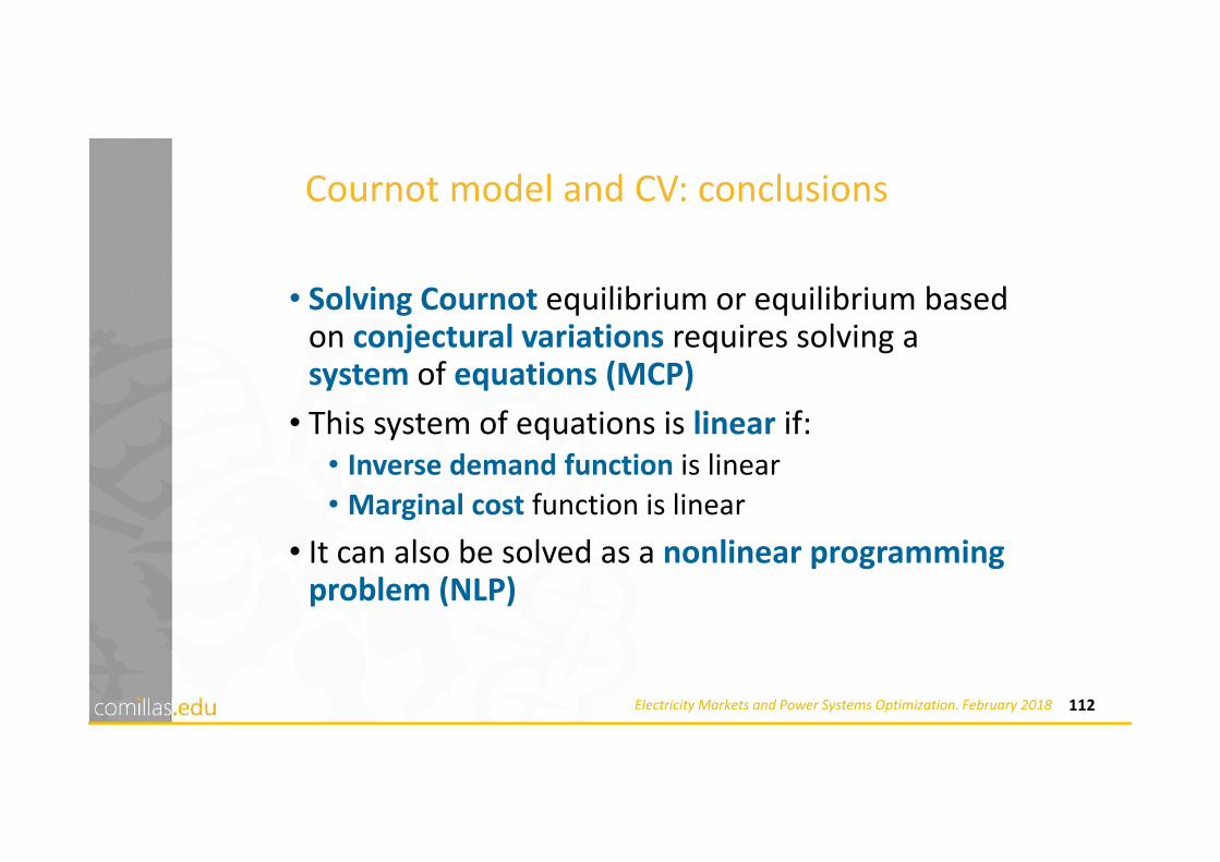
Cournot model and CV: conclusions
• Solving Cournot equilibrium or equilibrium based on conjectural variations requires solving a system of equations (MCP)
• This system of equations is linear if:
• Inverse demand function is linear
• Marginal cost function is linear
• It can also be solved as a nonlinear programming problem (NLP)

3.3
Bushnell model
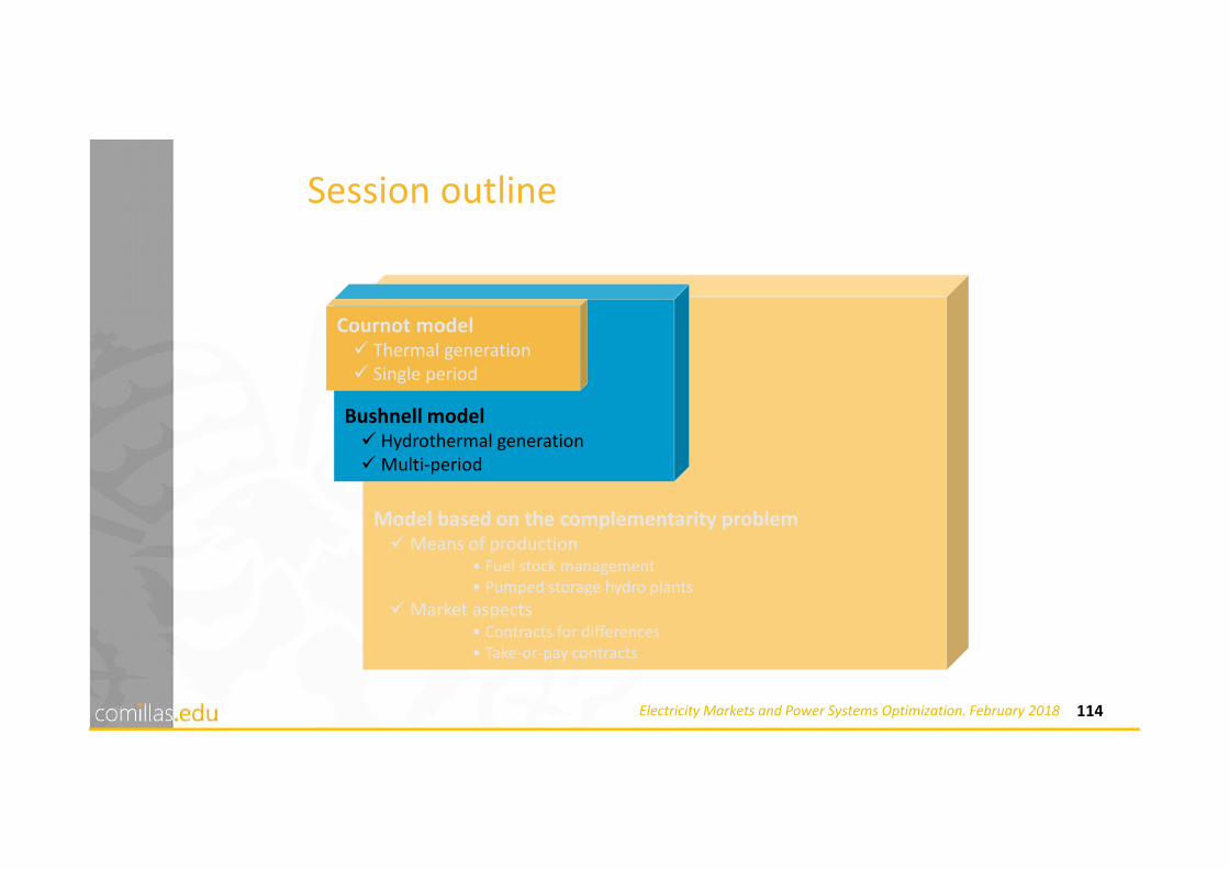
114Electricity Markets and Power Systems Optimization. February 2018
Model based on the complementarity problem Means of production
• Fuel stock management
• Pumped storage hydro plants
Market aspects• Contracts for differences
• Take-or-pay contracts
Session outline
Bushnell model Hydrothermal generation
Multi-period
Cournot model Thermal generation
Single period
115Electricity Markets and Power Systems Optimization. February 2018
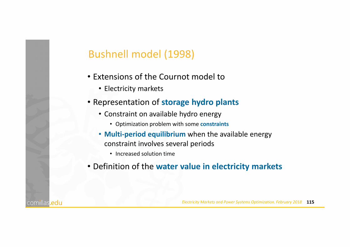
Bushnell model (1998)
• Extensions of the Cournot model to
• Electricity markets
• Representation of storage hydro plants
• Constraint on available hydro energy
• Optimization problem with some constraints
• Multi-period equilibrium when the available energy
constraint involves several periods
• Increased solution time
• Definition of the water value in electricity markets
116Electricity Markets and Power Systems Optimization. February 2018
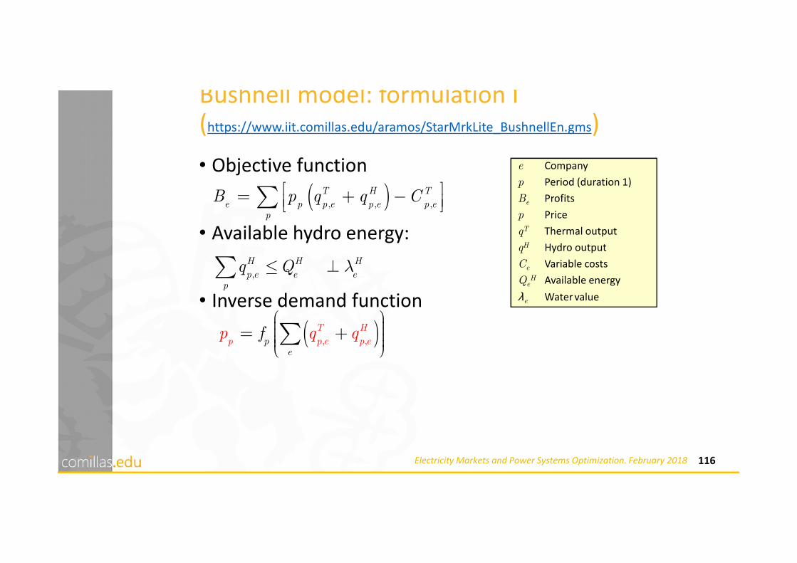
Bushnell model: formulation I(https://www.iit.comillas.edu/aramos/StarMrkLite_BushnellEn.gms)
• Objective function
• Available hydro energy:
• Inverse demand function
( ), , ,
T H T
e p p e p e p ep
B p q q C = + − ∑
,
H H H
p e e ep
q Q λ≤ ⊥∑
e Company
p Period (duration 1)
Be Profits
p Price
qT Thermal output
qH Hydro output
Ce Variable costs
QeH Available energy
λe Water value
( ), ,
T H
pe
p p e p ep qf q
= + ∑

117Electricity Markets and Power Systems Optimization. February 2018
Bushnell model: formulation II
• Lagrangian function (equivalent optimization
problem but without constraints)
• Optimality conditions
( ) ( )
( )
, ,
,
,
,
, , ,
, ,
0
0
T H T
p p e p e p
Te
p e p p eT
p e
e
p e pH
p e
e
T H H
p p e p e e
MR p MCq
MR
p q q q
p pq
q q
∂
∂
∂λ
∂
′= → = + + =
′= → = + + =−
L
L
e Company
p Period (duration 1)
Be Profits
p Price
qT Thermal output
qH Hydro output
Ce Variable costs
QeH Available energy
λe Water value
MCe Marginal cost
MRe Marginal revenue
( ) ( ), , , ,
,
T H T T
e p p e p e p e p ep
H H H
e p e ep
p q q C q
q Qλ
= + − + −
∑
∑
L

118Electricity Markets and Power Systems Optimization. February 2018
Bushnell model: comments
• The "Bushnell conjecture" is the Cournot conjecture extended to all the periods (e* = all other companies)
• Qualitative conclusions are drawn from the optimality conditions
• Total optimal output (as in Cournot)
• Water value
( ),e
,
,
, ,0
T
p p eT H
p e p e
T
p e
T
pp e
p qq
MC
pq
q
∂
∂
−= → + =
′−
L
e e
, ,
, ,
0; 0 T
p e p eT H
p e
H
p e
eMR MC
q q∂ ∂λ
∂ ∂= = → = =−
L L
, **
,
0p e
e
p e
q
q
′∂=
∂
∑

119Electricity Markets and Power Systems Optimization. February 2018
Water value in electricity markets
• Very important concept in hydrothermal coordination
• Final decision on hydro output
• The objective function changes when the amount of hydro energy available increases
• In centralized planning• Reduces system operating costs
• In electricity markets• Increases in each company’s profits
• Calculated as the dual variable of the available hydro energy constraint
120Electricity Markets and Power Systems Optimization. February 2018
Water value: Bushnell model
• Hydro output attempts to equal inter-period marginal
revenues
• Each company regards its water to be marginal revenue,
whose value coincides with the marginal cost of its thermal
plant
• Intuitively, when a company replaces 1 MW of thermal
output with 1 MW of hydro generation, the savings equal its
marginal cost
e e, ,
, ,
0; 0 T H
p e p e eT H
p e p e
MR MCq q
∂ ∂λ
∂ ∂= = → = =−
L L
( ), ,
, ,
T T
p p e p eT H
p e p e
p
p MC qq q
p
−+ =
′−
121Electricity Markets and Power Systems Optimization. February 2018
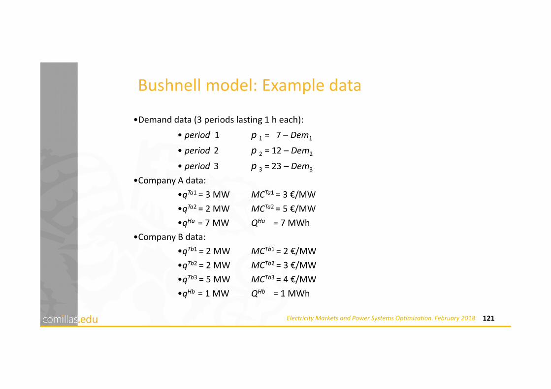
Bushnell model: Example data
•Demand data (3 periods lasting 1 h each):
• period 1 p 1 = 7 – Dem1
• period 2 p 2 = 12 – Dem2
• period 3 p 3 = 23 – Dem3
•Company A data:
•qTa1 = 3 MW MCTa1 = 3 €/MW
•qTa2 = 2 MW MCTa2 = 5 €/MW
•qHa = 7 MW QHa = 7 MWh
•Company B data:
•qTb1 = 2 MW MCTb1 = 2 €/MW
•qTb2 = 2 MW MCTb2 = 3 €/MW
•qTb3 = 5 MW MCTb3 = 4 €/MW
•qHb = 1 MW QHb = 1 MWh
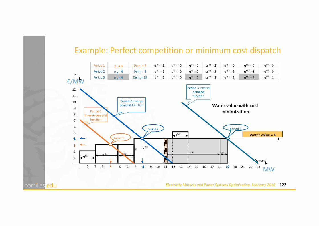
122Electricity Markets and Power Systems Optimization. February 2018
4 8
3
4
19
Example: Perfect competition or minimum cost dispatch
Period 1 p1 = 3 Dem1 = 4 qTa1 = 2 qTa2 = 0 qHa = 0 qTb1 = 2 qTb2 = 0 qTb3 = 0 qHb = 0
Period 2 p 2 = 4 Dem2 = 8 qTa1 = 3 qTa2 = 0 qHa = 0 qTb1 = 2 qTb2 = 2 qTb3 = 1 qHb = 0
Period 3 p 3 = 4 Dem3 = 19 qTa1 = 3 qTa2 = 0 qHa = 7 qTb1 = 2 qTb2 = 2 qTb3 = 4 qHb = 1p
qTb1
Demand
7
2
10
6 13 171072 3 51 9 11 12 15 1614
6
5
8
9
1
11
12Period 3 inverse
demand
function
Water value with cost
minimization
qTa1 qTb2
qTb3
2318 21 2220
qHb
Period 1
inverse demand
function
Period 1
3
4
qTa2
qHa
4
Period 3
19
Water value = 4
Period 2 inverse
demand function
Period 2
4
8
€/MW
MW
123Electricity Markets and Power Systems Optimization. February 2018
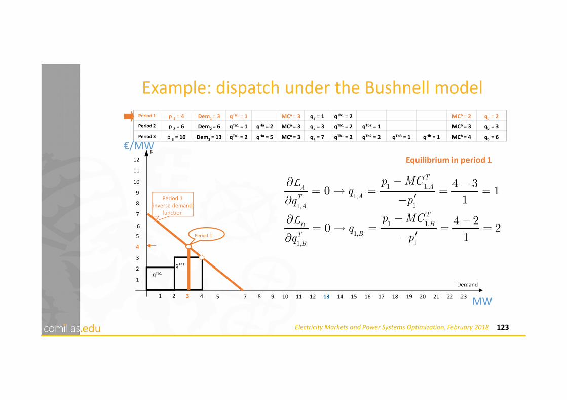
Example: dispatch under the Bushnell model
Period 1 p 1 = 4 Dem1 = 3 qTa1 = 1 MCa = 3 qa = 1 qTb1 = 2 MCb = 2 qb = 2
Period 2 p 2 = 6 Dem2 = 6 qTa1 = 1 qHa = 2 MCa = 3 qa = 3 qTb1 = 2 qTb2 = 1 MCb = 3 qb = 3
Period 3 p 3 = 10 Dem3 = 13 qTa1 = 2 qHa = 5 MCa = 3 qa = 7 qTb1 = 2 qTb2 = 2 qTb3 = 1 qHb = 1 MCb = 4 qb = 6
qTa1
3
p
qTb1
Demand
7
2
10
5
8
9
1
11
12 Equilibrium in period 1
4 8 1913 171072 51 9 11 12 15 1614 2318 21 2220
Period 1
4
Period 1
inverse demand
function
3
6
€/MW
MW
1 1,
1,
11,
1 1,
1,
11,
4 30 1
1
4 20 2
1
T
AA
AT
A
T
BB
BT
B
p MCq
pq
p MCq
pq
∂
∂
∂
∂
− −= → = = =
′−
− −= → = = =
′−
L
L

124Electricity Markets and Power Systems Optimization. February 2018
Example: dispatch under the Bushnell model
qTa1
3
p
qTb1
qTb2qHa
Demand
7
2
10
5
8
9
1
11
12 Equilibrium in period 2
4 8 19
Period 2
6
Period 2
inverse demand
function
6 13 171072 51 9 11 12 15 1614 2318 21 2220
4
3
Period 1 p 1 = 4 Dem1 = 3 qTa1 = 1 MCa = 3 qa = 1 qTb1 = 2 MCb = 2 qb = 2
Period 2 p 2 = 6 Dem2 = 6 qTa1 = 1 qHa = 2 MCa = 3 qa = 3 qTb1 = 2 qTb2 = 1 MCb = 3 qb = 3
Period 3 p 3 = 10 Dem3 = 13 qTa1 = 2 qHa = 5 MCa = 3 qa = 7 qTb1 = 2 qTb2 = 2 qTb3 = 1 qHb = 1 MCb = 4 qb = 6
qTb3
2 2,A2,
22,
6 30 3
1
T
A
AT
A
p CMq
pq
∂
∂
− −= → = = =
′−
L
2 2,B2,
22,
6 30 3
1
T
B
BT
B
p CMq
pq
∂
∂
− −= → = = =
′−
L
€/MW
MW

125Electricity Markets and Power Systems Optimization. February 2018
Example: dispatch under the Bushnell model
qTa1
qTb3
3
p
qTb1
qHb
Demand
7
2
10
5
8
9
1
11
12 Equilibrium in period 3
qHaqTb2
4 8 19
6
6 13 171072 51 9 11 12 15 1614 2318 21 2220
Period 3
Period 3
inverse demand
function
4
3
Period 1 p 1 = 4 Dem1 = 3 qTa1 = 1 MCa = 3 qa = 1 qTb1 = 2 MCb = 2 qb = 2
Period 2 p 2 = 6 Dem2 = 6 qTa1 = 1 qHa = 2 MCa = 3 qa = 3 qTb1 = 2 qTb2 = 1 MCb = 3 qb = 3
Period 3 p 3 = 10 Dem3 = 13 qTa1 = 2 qHa = 5 MCa = 3 qa = 7 qTb1 = 2 qTb2 = 2 qTb3 = 1 qHb = 1 MCb = 4 qb = 6
3 3,A
3,
33,
10 30 7
1
T
A
AT
A
p CMq
pq
∂
∂
− −= → = = =
′−
L
3 3,B3,
33,
10 40 6
1
T
B
BT
B
p CMq
pq
∂
∂
− −= → = = =
′−
L
€/MW
MW

126Electricity Markets and Power Systems Optimization. February 2018
Example: dispatch under the Bushnell model
qTa1
qTb3
3
p
qTb1
qHb
Demand
7
2
10
5
8
9
1
11
12
Water value
qHaqTb2
4 8 19
6
6 13 171072 51 9 11 12 15 1614 2318 21 2220
Period 3
Period 3
inverse demand
function
4
3
Water value for company A = 3
Water value for company B = 4
Period 1 p 1 = 4 Dem1 = 3 qTa1 = 1 MCa = 3 qa = 1 qTb1 = 2 MCb = 2 qb = 2
Period 2 p 2 = 6 Dem2 = 6 qTa1 = 1 qHa = 2 MCa = 3 qa = 3 qTb1 = 2 qTb2 = 1 MCb = 3 qb = 3
Period 3 p 3 = 10 Dem3 = 13 qTa1 = 2 qHa = 5 MCa = 3 qa = 7 qTb1 = 2 qTb2 = 2 qTb3 = 1 qHb = 1 MCb = 4 qb = 6
€/MW
MW

127Electricity Markets and Power Systems Optimization. February 2018
Bushnell model: conclusions
• Solving Bushnell equilibrium (without less than or equal to constraints) entails solving a multi-period system of equations
• The system of equations is linear if:
• Inverse demand function is linear
• Marginal cost function is linear
128Electricity Markets and Power Systems Optimization. February 2018
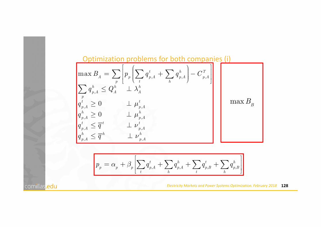
Optimization problems for both companies (i)
, , ,
,
, ,
, ,
, ,
, ,
max
0
0
t h T
A p p A p A p Ap t h
h h h
p A A Ap
t t
p A p A
h h
p A p A
t t t
p A p A
h h h
p A p A
B p q q C
q Q
q
q
q q
q q
λ
µ
µ
ν
ν
= + − ≤ ⊥
≥ ⊥
≥ ⊥
≤ ⊥
≤ ⊥
∑ ∑ ∑∑
, , , ,
t h t h
p p p p A p A p B p Bt h t h
p q q q qα β = + + + + ∑ ∑ ∑ ∑
maxBB

129Electricity Markets and Power Systems Optimization. February 2018
Optimization problems for both companies (ii)
, , , ,
, , , , , , , ,
, , , ,, , 0; , 0
t h T h h h
A p p A p A p A A p A Ap t h p
t t h h t t t h h h
p A p A p A p A p A p A p A p A
h t h t h
A p A p A p A p A
p q q C q Q
q q q q q q
λ
µ µ ν ν
λ ν ν µ µ
= − + − + − + + + + − + −
≥ ≤
∑ ∑ ∑ ∑L
, , , ,
t h t h
p p p p A p A p B p Bt h t h
p q q q qα β = + + + + ∑ ∑ ∑ ∑
BL
Minimization

130Electricity Markets and Power Systems Optimization. February 2018
Optimization problems for both companies (iii)
, , ,
,
, ,
,
,
, ,
, ,
0
0
0
0; 0
0;
t h T t tA
p p p A p A p A p ptt hp A
t h h t tA
p p p A p A A p pht hp A
h h h
A p A Ap
t t h h
p p A p p A
t t t h h h
p p A p p A
p p q q MCq
p p q qq
q Q
q q
q q q q
µ ν
λ µ ν
λ
µ µ
ν ν
∂ ′= − − + + + + = ∂ ∂ ′= − − + + + + = ∂
− =
= = − = − =
∑ ∑
∑ ∑
∑
L
L
, , , ,
0
, , 0; , 0
t h t h
p p p p A p A p B p Bt h t h
h t h t h
p p p p
p q q q qα β
λ ν ν µ µ
= + + + +
≥ ≤
∑ ∑ ∑ ∑

4
Decision Support Models
1. Power Systems
2. Optimization
3. Electricity Markets
4. Decision Support Models

132Electricity Markets and Power Systems Optimization. February 2018
Decision Support Tool or Model• Definition
- Simplified description, especially a mathematical one, of asystem or process, to assist calculations and predictions. (Oxford
Dictionary)
• Accurate representation of a reality
• May involve a multidisciplinary team
• Balance between a detailed representation and the skill to obtain a solution

133Electricity Markets and Power Systems Optimization. February 2018
• Managers (decision makers)• Are the most involved with the problem and have preferences about how the solution should
be.
• Have less knowledge about the formulation and solution techniques that could be applied: “do the same as last time because we are too busy to devise a different way”
• Software expert• Might have experience with standard formulations, modifying general purpose solution
algorithms, commercial software and IT issues
• Have less knowledge about the particular problem: “buy a good package and apply it”
• OR/MS analyst (*):• Has some knowledge of the problem and its context.
• Knows the techniques that can help to solve it and might have multi-industry and multi-discipline experience: “understand the problem and fit or devise a technique for it”
• Academic or consulting environment (e.g., IIT)
• Tailor made tool
(*) OR/MS: “Operations research” and “management science” are terms that are used interchangeably to describe the discipline of applying advanced analytical techniques to help make better decisions and to solve problems.
Model development team
134Electricity Markets and Power Systems Optimization. February 2018
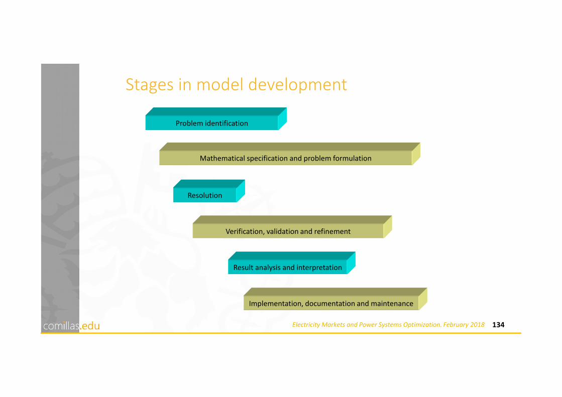
Stages in model development
Problem identification
Mathematical specification and problem formulation
Resolution
Verification, validation and refinement
Result analysis and interpretation
Implementation, documentation and maintenance

135Electricity Markets and Power Systems Optimization. February 2018
Hierarchy of Operation Planning ModelsST AR T
E N D
Stochastic M arke t
Equ ilib r ium Mode l
S tochastic M arke tEqu ilib r ium Mode l
Hyd ro the rm a l
Coo rdina tion M ode l
Hyd ro the rm a l
Coo rdina tion M ode l
Stochastic
S im ula tion Mode l
S tochas tic
S im ulation Mode l
M onth ly hyd ro basin and
the rm a l p lant p roduction
W eekly hyd ro un it
p roduction
D a il y hyd ro un it
p roduction
C oherence?
Adju
stm
en
t
Adju
stm
en
t
yes
no
U n it Com m itm en t
O ff er ing S trateg ies
U n it Com m itm en t
O ffer ing S trateg ies
ST AR T
E N D
Stochastic M arke t
Equ ilib r ium Mode l
S tochastic M arke tEqu ilib r ium Mode l
Hyd ro the rm a l
Coo rdina tion M ode l
Hyd ro the rm a l
Coo rdina tion M ode l
Stochastic
S im ula tion Mode l
S tochas tic
S im ulation Mode l
M onth ly hyd ro basin and
the rm a l p lant p roduction
W eekly hyd ro un it
p roduction
D a il y hyd ro un it
p roduction
C oherence?
Adju
stm
en
t
Adju
stm
en
t
yes
no
U n it Com m itm en t
O ff er ing S trateg ies
U n it Com m itm en t
O ffer ing S trateg ies

4.1
MOES Stochastic
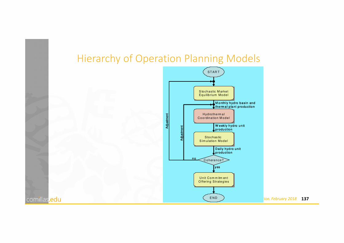
137Electricity Markets and Power Systems Optimization. February 2018
Hierarchy of Operation Planning ModelsST AR T
E N D
Stochastic M arke t
Equ ilib r ium Mode l
S tochastic M arke tEqu ilib r ium Mode l
Hyd ro the rm a l
Coo rdina tion M ode l
Hyd ro the rm a l
Coo rdina tion M ode l
Stochastic
S im ula tion Mode l
S tochas tic
S im ulation Mode l
M onth ly hyd ro basin and
the rm a l p lant p roduction
W eekly hyd ro un it
p roduction
D a il y hyd ro un it
p roduction
C oherence?
Adju
stm
en
t
Adju
stm
en
t
yes
no
U n it Com m itm en t
O ff er ing S trateg ies
U n it Com m itm en t
O ffer ing S trateg ies
ST AR T
E N D
Stochastic M arke t
Equ ilib r ium Mode l
S tochastic M arke tEqu ilib r ium Mode l
Hyd ro the rm a l
Coo rdina tion M ode l
Hyd ro the rm a l
Coo rdina tion M ode l
Stochastic
S im ula tion Mode l
S tochas tic
S im ulation Mode l
M onth ly hyd ro basin and
the rm a l p lant p roduction
W eekly hyd ro un it
p roduction
D a il y hyd ro un it
p roduction
C oherence?
Adju
stm
en
t
Adju
stm
en
t
yes
no
U n it Com m itm en t
O ff er ing S trateg ies
U n it Com m itm en t
O ffer ing S trateg ies
138Electricity Markets and Power Systems Optimization. February 2018
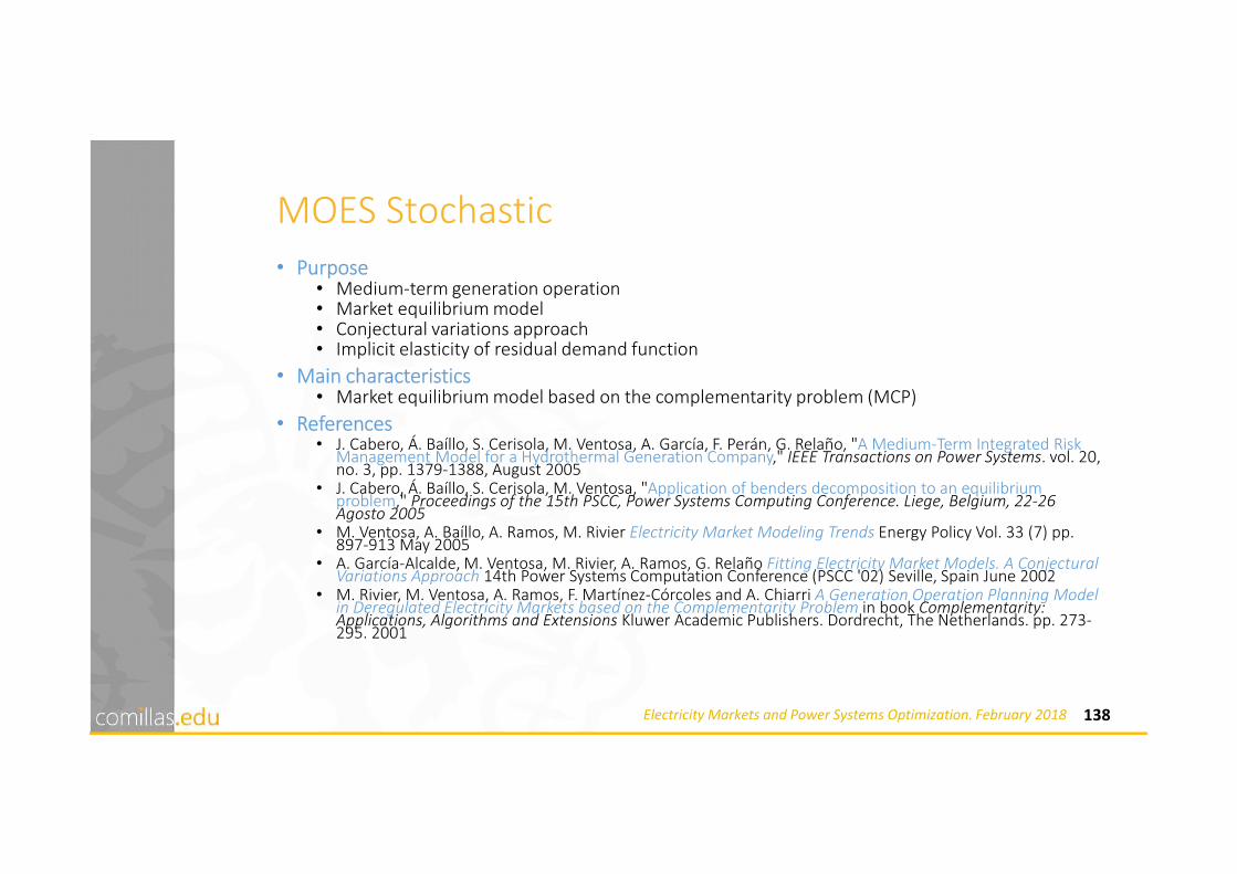
MOES Stochastic• Purpose
• Medium-term generation operation• Market equilibrium model• Conjectural variations approach• Implicit elasticity of residual demand function
• Main characteristics• Market equilibrium model based on the complementarity problem (MCP)
• References• J. Cabero, Á. Baíllo, S. Cerisola, M. Ventosa, A. García, F. Perán, G. Relaño, "A Medium-Term Integrated Risk
Management Model for a Hydrothermal Generation Company," IEEE Transactions on Power Systems. vol. 20, no. 3, pp. 1379-1388, August 2005
• J. Cabero, Á. Baíllo, S. Cerisola, M. Ventosa, "Application of benders decomposition to an equilibrium problem," Proceedings of the 15th PSCC, Power Systems Computing Conference. Liege, Belgium, 22-26 Agosto 2005
• M. Ventosa, A. Baíllo, A. Ramos, M. Rivier Electricity Market Modeling Trends Energy Policy Vol. 33 (7) pp. 897-913 May 2005
• A. García-Alcalde, M. Ventosa, M. Rivier, A. Ramos, G. Relaño Fitting Electricity Market Models. A Conjectural Variations Approach 14th Power Systems Computation Conference (PSCC '02) Seville, Spain June 2002
• M. Rivier, M. Ventosa, A. Ramos, F. Martínez-Córcoles and A. Chiarri A Generation Operation Planning Model in Deregulated Electricity Markets based on the Complementarity Problem in book Complementarity: Applications, Algorithms and Extensions Kluwer Academic Publishers. Dordrecht, The Netherlands. pp. 273-295. 2001
139Electricity Markets and Power Systems Optimization. February 2018
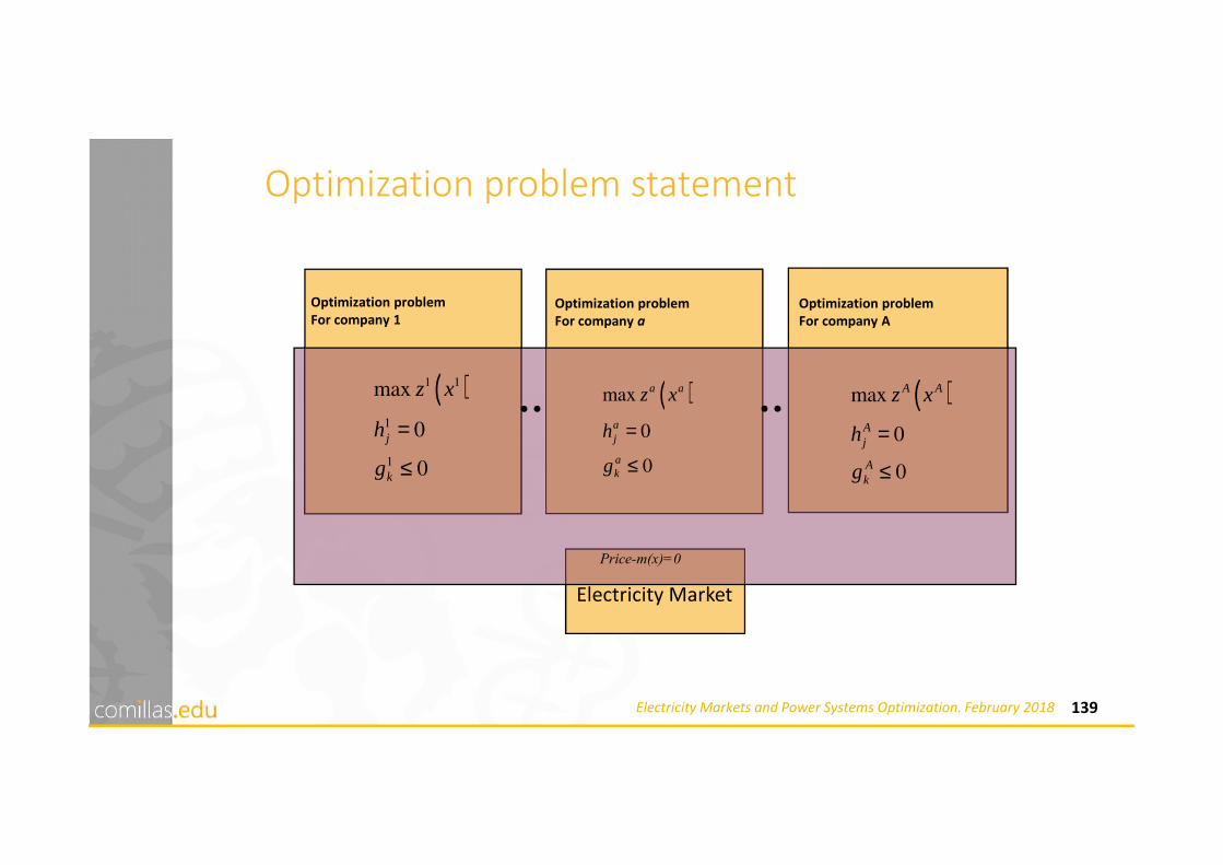
Optimization problem statement
( )max
0
0
e e
e
j
e
k
z x
h
g
=
≤
( )max
0
0
e e
e
j
e
k
z x
h
g
=
≤
( )max
0
0
e e
e
j
e
k
z x
h
g
=
≤
Electricity Market
Price-m(x)=0
Optimization problem
For company 1
( )1 1
1
1
max
0
0
j
k
z x
h
g
=
≤
Optimization problem
For company A
Optimization problem
For company a
( )max
0
0
a a
a
j
a
k
z x
h
g
=
≤
( )max
0
0
A A
A
j
A
k
z x
h
g
=
≤
140Electricity Markets and Power Systems Optimization. February 2018
Problem statement for each company
( )max
0
0
e e
e
j
e
k
z x
h
g
=
≤
( )max
0
0
e e
e
j
e
k
z x
h
g
=
≤
( )max
0
0
e e
e
j
e
k
z x
h
g
=
≤
Electricity Market
Price-m(x)=0
Optimization problem
For company 1
( )1 1
1
1
max
0
0
j
k
z x
h
g
=
≤
Optimization problem
For company A
Optimization problem
For company a
( )max
0
0
a a
a
j
a
k
z x
h
g
=
≤
( )max
0
0
A A
A
j
A
k
z x
h
g
=
≤
Objective Function
Maximization of:
Company profit for the problem scope
• Other revenues
• CTC’s
• Long term contracts...
• Price equation
• Interperiod
• Fuel management
• Hydro reservoir scheduling
• Intraperiod
• Weekly pumping
• Operational constraints
Technical constraints
Restricciones del Mercado
Subject to:

141Electricity Markets and Power Systems Optimization. February 2018
Practical difficulties• Good theoretical statement
• However, no solver available to solve such mathematical problem:
• Several optimization problems tied by price variable
• Look for another equivalent mathematical problem
• With the same solution values
• Numerically solvable
• Several alternatives
• Complementarity problem [Ventosa, Hobbs]
• Equivalent quadratic problem [Barquín, Hobbs]

142Electricity Markets and Power Systems Optimization. February 2018
Practical difficulties. Alternative approaches• Complementarity problem
• M. Rivier, M. Ventosa, A. Ramos A Generation Operation Planning Model in Deregulated Electricity Markets based on the Complementarity Problem 2nd International Conference on Complementarity Problems (ICCP 99) Madison, WI, USA June 1999
• B.F. Hobbs. “LCP Models of Nash – Cournot Competition in Bilateral and POOLCO–Based Power Markets.” In Proc. IEEE Winter Meeting, New York, 1999
• Equivalent quadratic system
• J. Barquín, E. Centeno, J. Reneses, "Medium-term generation programming in competitive environments: A new optimization approach for market equilibrium computing", IEE Proceedings-Generation Transmission and Distribution. vol. 151, no. 1, pp. 119-126, Enero2004.
• B.F. Hobbs. “Linear Complementarity Models of Nash–Cournot competition in Bilateral and POOLCO Power Markets” IEEE Transactions on Power Systems, 16 (2), May 2001
• Variational inequalities
• W. Jing-Yuan and Y. Streets, “Spatial oligopolistic electricity models with Cournot generators and regulated transmission prices,” Operations Res., vol. 47, no. 1, pp. 102–112, 1999

149Electricity Markets and Power Systems Optimization. February 2018
Electric power market
Equivalent mixed complementarity problem for all the companies
Price-m(y)=0
Company 1’s optimality conditions
Company E’s optimality conditions
Company e’s optimality conditions
( )
( )
11
1
11 1
1
1 1 1 1
, , 0
, , 0
0 0 0
x
j
j
k k k k
xx
x h
g g
λ
λ µ
λ µµ
λ λ
∂∇ = =∂
∂∇ = = =∂
⋅ = ≤ ≤
LL
LL
( )
( )
, , 0
, , 0
0 0 0
ee
x e
ee e
je
j
e e e e
k k k k
xx
x h
g g
λ
λ µ
λ µµ
λ λ
∂∇ = =∂
∂∇ = = =∂
⋅ = ≤ ≤
LL
LL
( )
( )
, , 0
, , 0
0 0 0
EE
x E
EE E
jE
j
E E E E
k k k k
xx
x h
g g
λ
λ µ
λ µµ
λ λ
∂∇ = =∂
∂∇ = = =∂
⋅ = ≤ ≤
LL
LL

150Electricity Markets and Power Systems Optimization. February 2018
Detailed system modeling (I)
• Market modeling
• Demand-side behavior
• Price is a linear function of demand
• Load-duration curve per period
• Cournot or CV company competition
• Simultaneous maximization of profits
• Market revenues are a quadratic function of price
• Other market characteristics
• Contracts for differences (sales)
• Take-or-pay contracts (purchase)

151Electricity Markets and Power Systems Optimization. February 2018
Detailed system modeling (II)
• Thermal generation
• Output limits
• Fuel consumption is quadratic
• Scheduled maintenance
• Deterministic modeling of unit outages
• Linear fuel stock management
• Hydro generation
• Storage hydro plants with reservoirs
• Run-of-the-river hydro plants
• Pumped storage hydro plants
• Linear reservoir management

152Electricity Markets and Power Systems Optimization. February 2018
Mixed linear complementarity problem (MLCP)
• Medium-term problem formulated with• linear constraints
• quadratic objective function
1max
2T Tc x x Qx
Ax b
Cx d
λ
µ
+
≤ ⊥
= ⊥
System of equations with a mixed linear complementarity problem structure
( )
0
0
0
T T
T
c Qx A C
Cx d
Ax b
Ax b
λ µ
λ
λ
+ + + = = ≤ ≤ − =
1max ( ) ( )
2T T T Tc x x Qx Ax b Cx dλ µ= + + − + −L
153Electricity Markets and Power Systems Optimization. February 2018
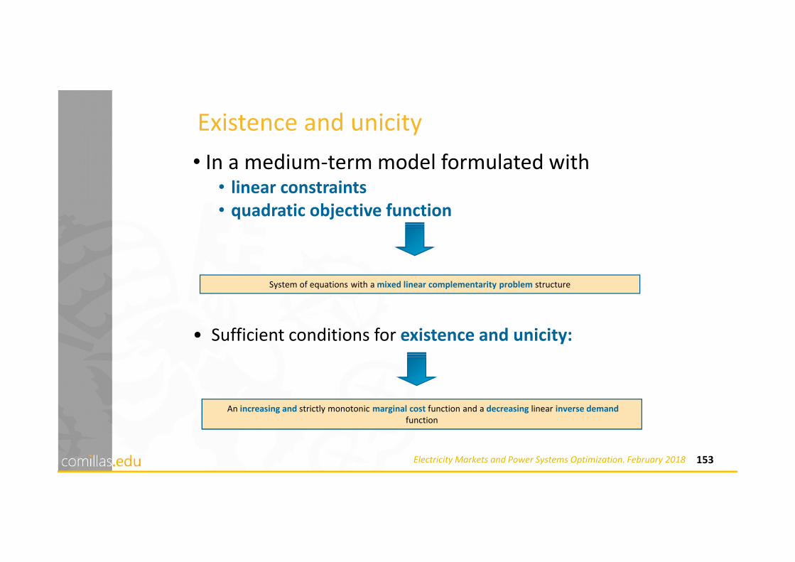
Existence and unicity
• In a medium-term model formulated with• linear constraints
• quadratic objective function
System of equations with a mixed linear complementarity problem structure
• Sufficient conditions for existence and unicity:
An increasing and strictly monotonic marginal cost function and a decreasing linear inverse demand
function

154Electricity Markets and Power Systems Optimization. February 2018
Stochastic optimization problem without risk
• Simultaneous agents’ stochastic optimization problems with price equation
Optimization
problem of company a
0 at t t t
a
α= − ⋅s S q
( )1max
subject to:
Operation constraints
E Π
Optimization
problem of company A
Optimization problem of company 1
( )max
subject to:
Operation constraints
aE Π ( )max
subject to:
Operation constraints
AE Π

4.2
MHE

162Electricity Markets and Power Systems Optimization. February 2018
Hierarchy of Operation Planning ModelsST AR T
E N D
Stochastic M arke t
Equ ilib r ium Mode l
S tochastic M arke tEqu ilib r ium Mode l
Hyd ro the rm a l
Coo rdina tion M ode l
Hyd ro the rm a l
Coo rdina tion M ode l
Stochastic
S im ula tion Mode l
S tochas tic
S im ulation Mode l
M onth ly hyd ro basin and
the rm a l p lant p roduction
W eekly hyd ro un it
p roduction
D a il y hyd ro un it
p roduction
C oherence?
Adju
stm
en
t
Adju
stm
en
t
yes
no
U n it Com m itm en t
O ff er ing S trateg ies
U n it Com m itm en t
O ffer ing S trateg ies
ST AR T
E N D
Stochastic M arke t
Equ ilib r ium Mode l
S tochastic M arke tEqu ilib r ium Mode l
Hyd ro the rm a l
Coo rdina tion M ode l
Hyd ro the rm a l
Coo rdina tion M ode l
Stochastic
S im ula tion Mode l
S tochas tic
S im ulation Mode l
M onth ly hyd ro basin and
the rm a l p lant p roduction
W eekly hyd ro un it
p roduction
D a il y hyd ro un it
p roduction
C oherence?
Adju
stm
en
t
Adju
stm
en
t
yes
no
U n it Com m itm en t
O ff er ing S trateg ies
U n it Com m itm en t
O ffer ing S trateg ies

163Electricity Markets and Power Systems Optimization. February 2018
Keys to success
• According to [Labadie, 2004] “the keys to success in implementation of reservoir system optimization models are:
• (1) improving the levels of trust by more interactive of decision makers in system development;
• (2) better “packaging” of these systems; and
• (3) improved linkage with simulation models which operators more readily accept”.

164Electricity Markets and Power Systems Optimization. February 2018
MHE
• Purpose• Determine the optimal yearly operation of all the thermal and hydro power plants• Medium term stochastic hydrothermal model for a complex multi-reservoir and multi-
cascaded hydro subsystem
• Main characteristics• General reservoir system topology• Cost minimization model• Thermal and hydro units considered individually• Nonlinear water head effects modeled for large reservoirs (NLP Problem)• Stochastic nonlinear optimization problem solved directed by a nonlinear solver given a close
initial solution provided by a linear solver
• References• A. Ramos, S. Cerisola, J.M. Latorre, R. Bellido, A. Perea, and E. Lopez A Decision Support Model for
Weekly Operation of Hydrothermal Systems by Stochastic Nonlinear Optimization in the book G. Consigli, M. Bertocchi and M.A.H. Dempster (eds.) Stochastic Optimization Methods in Finance and Energy. Springer 2011 ISBN 9781441995858 (Table of contents) 10.1007/978-1-4419-9586-5_7

166Electricity Markets and Power Systems Optimization. February 2018
Hydro subsystem• Different modeling approach for hydro reservoirs
depending on:• Owner company• Relevance of the reservoir
• Reservoirs belonging to other companies modeled in energy units [GWh]
• Own reservoirs modeled in water units [hm3, m3/s]
• Important reservoirs modeled with water head effects
• Very diverse hydro subsystem:• Hydro reservoir volumes from 0.15 to 2433 hm3
• Hydro plant capacities from 1.5 to 934 MW
169Electricity Markets and Power Systems Optimization. February 2018
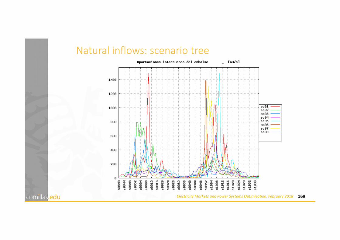
Natural inflows: scenario tree

179Electricity Markets and Power Systems Optimization. February 2018
Solution algorithm• Algorithm:
• Successive LP
• Direct solution by a NLP solver
• Very careful implementation
• Natural scaling of variables
• Use of simple expressions
• Initial values and bounds for all the nonlinear variables computed from the solution provided by linear solver (CPLEX 10.2 IPM)
• Nonlinear solvers
• CONOPT 3.14 [Generalized Reduced Gradient Method]
• KNITRO 5.1.0 [Interior-Point or an Active-Set Method]
• MINOS 5.51 [Project Lagrangian Algorithm]
• IPOPT 3.3 [Primal-Dual Interior Point Filter Line Search Algorithm]
• SNOPT 7.2-4 [Sequential Quadratic Programming Algorithm]
180Electricity Markets and Power Systems Optimization. February 2018
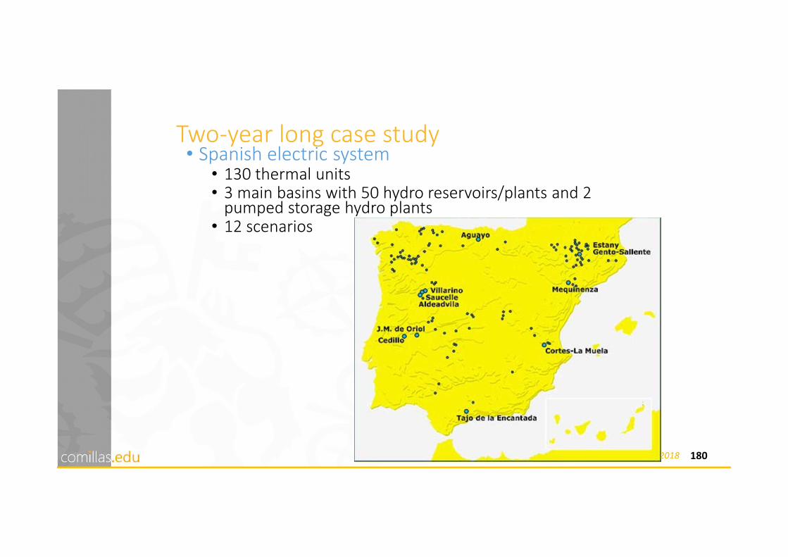
Two-year long case study• Spanish electric system
• 130 thermal units• 3 main basins with 50 hydro reservoirs/plants and 2
pumped storage hydro plants• 12 scenarios

4.3
Simulador

182Electricity Markets and Power Systems Optimization. February 2018
Hierarchy of Operation Planning ModelsST AR T
E N D
Stochastic M arke t
Equ ilib r ium Mode l
S tochastic M arke tEqu ilib r ium Mode l
Hyd ro the rm a l
Coo rdina tion M ode l
Hyd ro the rm a l
Coo rdina tion M ode l
Stochastic
S im ula tion Mode l
S tochas tic
S im ulation Mode l
M onth ly hyd ro basin and
the rm a l p lant p roduction
W eekly hyd ro un it
p roduction
D a il y hyd ro un it
p roduction
C oherence?
Adju
stm
en
t
Adju
stm
en
t
yes
no
U n it Com m itm en t
O ff er ing S trateg ies
U n it Com m itm en t
O ffer ing S trateg ies
ST AR T
E N D
Stochastic M arke t
Equ ilib r ium Mode l
S tochastic M arke tEqu ilib r ium Mode l
Hyd ro the rm a l
Coo rdina tion M ode l
Hyd ro the rm a l
Coo rdina tion M ode l
Stochastic
S im ula tion Mode l
S tochas tic
S im ulation Mode l
M onth ly hyd ro basin and
the rm a l p lant p roduction
W eekly hyd ro un it
p roduction
D a il y hyd ro un it
p roduction
C oherence?
Adju
stm
en
t
Adju
stm
en
t
yes
no
U n it Com m itm en t
O ff er ing S trateg ies
U n it Com m itm en t
O ffer ing S trateg ies
183Electricity Markets and Power Systems Optimization. February 2018
Simulador• Purpose
• Analyze and test different management strategies of hydro plants• Economic planning of hydro operation:
• Yearly and monthly planning• Update the yearly forecast:
• Operation planning up to the end of the year• Short term detailed operation:
• Detailed operation analysis of floods and droughts, changes in irrigation or recreational activities, etc.
• Main characteristics• Simulation technique• It has been proposed a general simulation method for hydro basins• A three phase method implements the maximize hydro production objective• Object Oriented Programming has been used• A flexible computer application implements this method
• References• J.M. Latorre, S. Cerisola, A. Ramos, R. Bellido, A. Perea Creation of Hydroelectric System Scheduling by
Simulation in the book H. Qudrat-Ullah, J.M. Spector and P. Davidsen (eds.) Complex Decision Making: Theoryand Practice pp. 83-96 Springer October 2007 ISBN 9783540736646 10.1007/978-3-540-73665-3_5
• J.M. Latorre, S. Cerisola, A. Ramos, A. Perea, R. Bellido Simulación de cuencas hidráulicas medianteProgramación Orientada a Objetos VIII Jornadas Hispano-Lusas de Ingeniería Eléctrica Marbella, España Julio 2005

184Electricity Markets and Power Systems Optimization. February 2018
Data representation (i)
• Basin topology is represented by a graph of nodes where each node is an element:
• Connections among nodes are physical junctions through the river.
• This structure induces the use of• Object Oriented Programming
Natural inflow
Reservoir
Hydro plant

185Electricity Markets and Power Systems Optimization. February 2018
Data representation (ii)• Five types of nodes (objects) are needed:
• Reservoir
• Channel
• Plant
• Inflow point
• River junction
• Each node is independently operated although it may require information from other elements
191Electricity Markets and Power Systems Optimization. February 2018
Reservoir operation strategies1. Optimal outflow decision taken from a
precalculated optimal water release table depending on:
• Week of the simulated day
• Hydrologic index of the basin inflows (type of year)
• Volume of the own reservoir
• Volume of a reference reservoir
• Table calculated by a long term hydrothermal model
• Usually for the main reservoirs of the basin
2. Outflow equals incoming inflow (usually for small
reservoirs)
3. Go to minimum target curve (spend as much as
possible)
4. Go to maximum target curve (keep water for the
future)

192Electricity Markets and Power Systems Optimization. February 2018
Simulation method (I)• Main objective:
• Maximize hydro production following the reservoir operation strategies
• Other objectives:• Avoid spillage
• Satisfaction of minimum outflow (irrigation)
• Proposed method requires three phases:1. Decides the initial management
2. Modifies it to avoid spillage and produce minimum outflows
3. Determines the electricity output for previous inflows
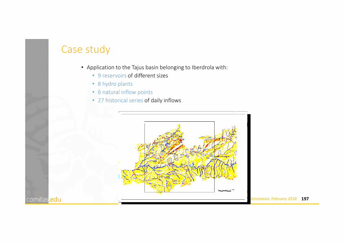
197Electricity Markets and Power Systems Optimization. February 2018
Case study
• Application to the Tajus basin belonging to Iberdrola with:
• 9 reservoirs of different sizes
• 8 hydro plants
• 6 natural inflow points
• 27 historical series of daily inflows

4.4
MAFO

199Electricity Markets and Power Systems Optimization. February 2018
Hierarchy of Operation Planning ModelsST AR T
E N D
Stochastic M arke t
Equ ilib r ium Mode l
S tochastic M arke tEqu ilib r ium Mode l
Hyd ro the rm a l
Coo rdina tion M ode l
Hyd ro the rm a l
Coo rdina tion M ode l
Stochastic
S im ula tion Mode l
S tochas tic
S im ulation Mode l
M onth ly hyd ro basin and
the rm a l p lant p roduction
W eekly hyd ro un it
p roduction
D a il y hyd ro un it
p roduction
C oherence?
Adju
stm
en
t
Adju
stm
en
t
yes
no
U n it Com m itm en t
O ff er ing S trateg ies
U n it Com m itm en t
O ffer ing S trateg ies
ST AR T
E N D
Stochastic M arke t
Equ ilib r ium Mode l
S tochastic M arke tEqu ilib r ium Mode l
Hyd ro the rm a l
Coo rdina tion M ode l
Hyd ro the rm a l
Coo rdina tion M ode l
Stochastic
S im ula tion Mode l
S tochas tic
S im ulation Mode l
M onth ly hyd ro basin and
the rm a l p lant p roduction
W eekly hyd ro un it
p roduction
D a il y hyd ro un it
p roduction
C oherence?
Adju
stm
en
t
Adju
stm
en
t
yes
no
U n it Com m itm en t
O ff er ing S trateg ies
U n it Com m itm en t
O ffer ing S trateg ies

200Electricity Markets and Power Systems Optimization. February 2018
MAFO• Purpose
• Short-term generation operation• Strategic Unit Commitment development of offering strategies• Daily and adjustment markets
• Main characteristics• Decomposition techniques (Benders, Lagrangian relaxation)
• References• A. Baillo, S. Cerisola, J. Fernandez-Lopez, A. Ramos Stochastic Power Generation Unit
Commitment in Electricity Markets: A Novel Formulation and A Comparison of Solution MethodsOperations Research (accepted) JCR impact factor 1.234 (2006)
• J.M. Fernandez-Lopez, Á. Baíllo, S. Cerisola, R. Bellido, "Building optimal offer curves for an electricity spot market: a mixed-integer programming approach," Proceedings of the 15th PSCC, Power Systems Computing Conference. Liege, Belgium, 22-26 Agosto 2005
• Á. Baíllo, M. Ventosa, M. Rivier, A. Ramos, "Optimal offering strategies for generation companies operating in electricity spot markets," IEEE Transactions on Power Systems. vol. 19, no. 2, pp. 745-753, May 2004
• A. Baíllo, M. Ventosa, M. Rivier, A. Ramos, G. Relaño Bidding in a Day-Ahead Electricity Market: A Comparison of Decomposition Techniques 14th Power Systems Computation Conference (PSCC '02) Seville, Spain June 2002
• A. Baíllo, M. Ventosa, A. Ramos, M. Rivier, A. Canseco Strategic unit commitment for generation companies in deregulated electricity markets in book The Next Generation of Electric Power Unit Commitment Models Kluwer Academic Publishers Boston, MA, USA pp. 227-248 2001

201Electricity Markets and Power Systems Optimization. February 2018
Curva esperada de demanda residual
0
20
40
60
80
100
120
6000 8000 10000 12000 14000 16000 18000
Energía (MWh)
Pre
cio
(€
/MW
h)
Modeling short term uncertainty: multistage approach
• Generation company doesn’t know the residual demand curve for each hour:

202Electricity Markets and Power Systems Optimization. February 2018
Curva esperada de demanda residual
0
20
40
60
80
100
120
6000 8000 10000 12000 14000 16000 18000
Energía (MWh)
Pre
cio
(€
/MW
h)
Modeling short term uncertainty: multistage approach
• Explicit recognition of uncertainty justifies the importance of offering strategies:
Posibles curvas de demanda residual
0
20
40
60
80
100
120
6000 8000 10000 12000 14000 16000 18000
Energía (MWh)
Pre
cio
(€
/MW
h)

203Electricity Markets and Power Systems Optimization. February 2018
Selling offers have to build an
increasing curve
Offering curve between two possible
realizations of residual demand curve
is irrelevant
Company decisions are reduced to chose
selling output for each residual demand
Modeling short term uncertainty: multistage approach
• Hypothesis: probability distribution of residualdemand curve has finite support:
Number of possible realizations of residual
demand curve is finite
Cantidad
Precio
( )1p q
1q 2q
( )2p q
3q
( )3p q

204Electricity Markets and Power Systems Optimization. February 2018
• Solution in two phases:• Stochastic unit commitment
• Optimal offering strategies under uncertainty.
• Structure of these problems.
• Possible decomposition techniques:• Benders.• Lagrangian relaxation.
Solution problem strategy

205Electricity Markets and Power Systems Optimization. February 2018
• Scope of short term decisions is one week:• Startup and shutdown planning: unit commitment.
• Daily hydro scheduling: hydrothermal coordination.
• This weekly problem can be seen as a sequence of two-stage stochastic problems, one for each day of the week.
First problem: weekly stochastic multistage planning

206Electricity Markets and Power Systems Optimization. February 2018
First problem: weekly stochastic multistage planning
Ofertas para el mercado diario
Casación mercado diario
Distribución de probabilidad discreta del mercado diario
Ofertas para el mercado de ajustes
Casación mercado ajustes
Resultado esperado para el mercado de ajustes
Programa de generación
Día 1
Ofertas para el mercado diario
Casación mercado diario
Distribución de probabilidad discreta del mercado diario
Ofertas para el mercado de ajustes
Casación mercado ajustes
Resultado esperado para el mercado de ajustes
Programa de generación
Día 2
Ofertas para el mercado diario
Casación mercado diario
Distribución de probabilidad discreta del mercado diario
Ofertas para el mercado de ajustes
Casación mercado ajustes
Resultado esperado para el mercado de ajustes
Programa de generación
Día 7

207Electricity Markets and Power Systems Optimization. February 2018
Ofertas para el mercado diario
Casación mercado diario
Distribución de probabilidad discreta del mercado diario
Ofertas para el mercado de ajustes
Casación mercado ajustes
Resultado esperado para el mercado de ajustes
Programa de generación
Día 1
Ofertas para el mercado diario
Casación mercado diario
Distribución de probabilidad discreta del mercado diario
Ofertas para el mercado de ajustes
Casación mercado ajustes
Resultado esperado para el mercado de ajustes
Programa de generación
Día 2
Ofertas para el mercado diario
Casación mercado diario
Distribución de probabilidad discreta del mercado diario
Ofertas para el mercado de ajustes
Casación mercado ajustes
Resultado esperado para el mercado de ajustes
Programa de generación
Día 7
First problem: detail for each day of the week
Ofertas para el
mercado diario
Casación
mercado
diario
Distribución de probabilidad
discreta del mercado diario
Ofertas para el
mercado de ajustes
Casación
mercado
ajustes
Resultado esperado para
el mercado de ajustes
Programa de
generación
Día 2
Ofertas para el
mercado diario
Casación
mercado
diario
Distribución de probabilidad
discreta del mercado diario
Ofertas para el
mercado de ajustes
Casación
mercado
ajustes
Resultado esperado para
el mercado de ajustes
Programa de
generación
Día 2
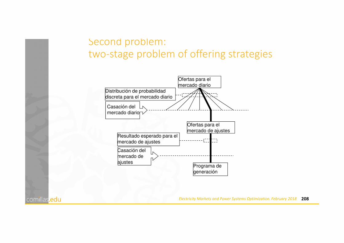
208Electricity Markets and Power Systems Optimization. February 2018
Second problem: two-stage problem of offering strategies
Ofertas para el
mercado diario
Casación del
mercado diario
Distribución de probabilidad
discreta para el mercado diario
Ofertas para el
mercado de ajustes
Casación del
mercado de
ajustes
Resultado esperado para el
mercado de ajustes
Programa de
generación

4.5
Other models

211Electricity Markets and Power Systems Optimization. February 2018
Market Equilibrium
Iberdrola Endesa Gas Natural
Fenosa E.ON
España Red
Eléctrica IIT
Back Office Long Term Expansion Planning
Generation and transmission
BEST MORSE
EXPANDE OWL
TEPES
Back Office Medium Term Operation Planning
Market Equilibrium MOES MPO VALORE MARAPE PLAMER PREMED
Hydro Subsystem MHE
Simulador EXLA
Renewable sources integration. EV, VPP MEMPHIS ROM
Transmission Network SIMUPLUS StarNet SECA
Generation reliability assessment FLOP
Front Office Short Term Offer Strategies and Operation Planning UC and operation reserves MAFO SGO GRIMEL

212Electricity Markets and Power Systems Optimization. February 2018
Valore• Purpose
• Oligolopolistic electricity markets simulation
• Main characteristics• Based on quadratic optimization (QP)
• Medium-term
• Allows detailed physical assets modeling
• Extended for stochastic optimization (i.e. water inflows)
• Network constraints (explicit and implicit transmission auctions)
• References• J. Barquín, M. Vázquez, Cournot Equilibrium Calculation in Power Networks: An
Optimization Approach With Price Response Computation, IEEE Trans. on Power Systems, 23, no. 2, 317-326, May, 2008
• J. Barquín, E. Centeno, J. Reneses , Stochastic Market Equilibrium Model For Generation Planning, Probability in the Engineering and Informational Sciences, 19, 533-546, August, 2005

213Electricity Markets and Power Systems Optimization. February 2018
Fuzzy Valore• Purpose
• Proposing an electricity market model based on the conjectural-price-response equilibrium when uncertainty of RDC is modeled using the possibility theory
• Main characteristics• Compute robust Cournot equilibrium by using possibilistic VAR for medium
term analysis• Determine possibility distributions of main outputs (prices and incomes)• Novel variational inequalities (VI) algorithms with global and proved
convergence that iteratively solve quadratic programming (QP) models
• References• F.A. Campos, J. Villar, J. Barquín, J. Reneses, "Variational inequalities for solving
possibilistic risk-averse electricity market equilibrium," IET Gener. Transm. Distrib. vol. 2, no. 5, pp. 632-645, Sep 2008
• F.A. Campos, J. Villar, J. Barquín, J. Ruipérez, "Robust mixed strategies in fuzzy non-cooperative Nash games," Engineering Optimization. vol. 40, no. 5, pp. 459-474, May 2008
• F.A. Campos, J. Villar, J. Barquín, "Application of possibility theory to robust Cournotequilibriums in electricity market," Probability in the Engineering and Informational Sciences. vol. 19, no. 4, pp. 519-531, October 2005
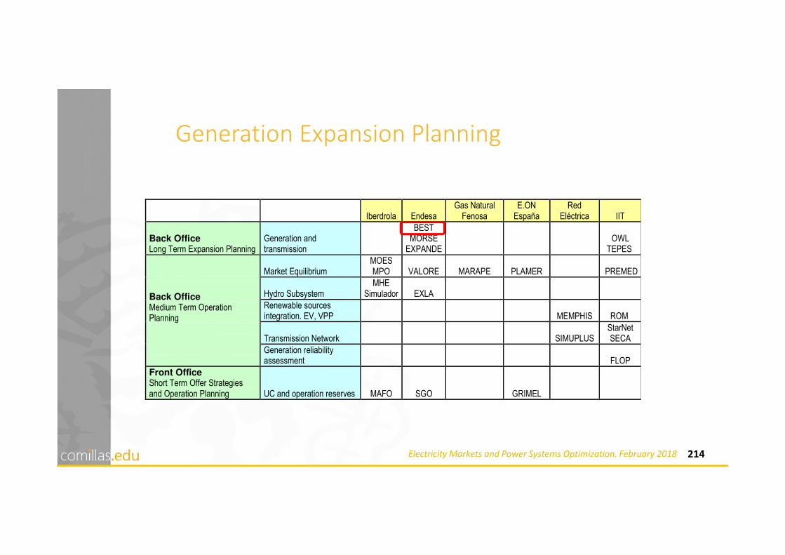
214Electricity Markets and Power Systems Optimization. February 2018
Generation Expansion Planning
Iberdrola Endesa Gas Natural
Fenosa E.ON
España Red
Eléctrica IIT
Back Office Long Term Expansion Planning
Generation and transmission
BEST MORSE
EXPANDE OWL
TEPES
Back Office Medium Term Operation Planning
Market Equilibrium MOES MPO VALORE MARAPE PLAMER PREMED
Hydro Subsystem MHE
Simulador EXLA
Renewable sources integration. EV, VPP MEMPHIS ROM
Transmission Network SIMUPLUS StarNet SECA
Generation reliability assessment FLOP
Front Office Short Term Offer Strategies and Operation Planning UC and operation reserves MAFO SGO GRIMEL

215Electricity Markets and Power Systems Optimization. February 2018
BEST• Purpose
• Assessment of investments in generation assets and other strategic decisions
• Main characteristics• Long-term scope (20-30 years)• System-dynamics based simulation (Business Dynamics)• Includes a detailed representation of agents’ market behavior based on
endogenously-computed conjectured price variation• Includes a detailed representation of decisions evaluation based on Merton-Black-
Scholes theory
• References• E. Centeno, J. Barquín, A. López-Peña, J.J. Sánchez, "Effects of gas-production constraints on
generation expansion," 16th Power Systems Computation Conference - PSCC 08. Glasgow,
Scotland, 14-18 Julio 2008
• J.J. Sánchez, J. Barquín, E. Centeno, "Fighting market power by auctioning generation: A system dynamics approach," INFORMS Annual Meeting 2007. Seattle, USA, 4-7 Noviembre 2007
• J.J. Sánchez, J. Barquín, E. Centeno, A. López-Peña, "System dynamics models for generation expansion planning in a competitive framework: Oligopoly and market power representation," Twenty-Fifth International System Dynamics Conference. Boston, Massachusetts, USA, 29 Julio-2
Agosto 2007
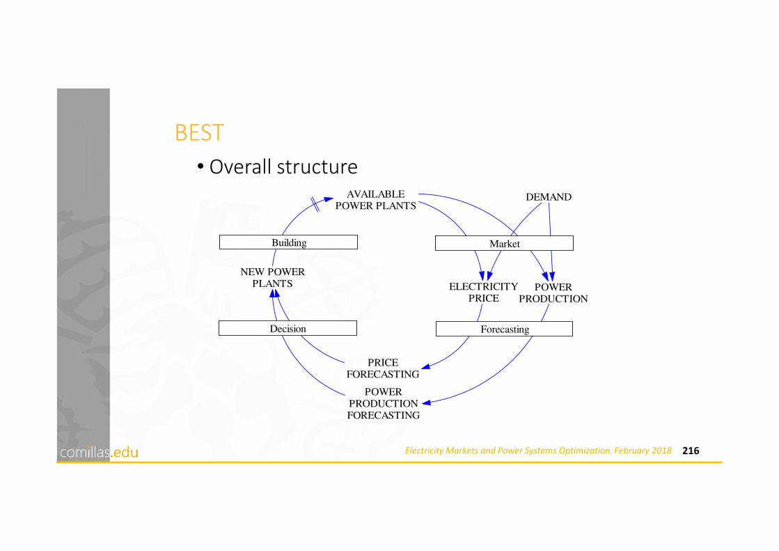
216Electricity Markets and Power Systems Optimization. February 2018
BEST
AVAILABLEPOWER PLANTS
ELECTRICITYPRICE
POWERPRODUCTION
PRICEFORECASTING
POWERPRODUCTIONFORECASTING
NEW POWERPLANTS
DEMAND
Building
ForecastingDecision
Market
• Overall structure

217Electricity Markets and Power Systems Optimization. February 2018
Hydro Scheduling
Iberdrola Endesa Gas Natural
Fenosa E.ON
España Red
Eléctrica IIT
Back Office Long Term Expansion Planning
Generation and transmission
BEST MORSE
EXPANDE OWL
TEPES
Back Office Medium Term Operation Planning
Market Equilibrium MOES MPO VALORE MARAPE PLAMER PREMED
Hydro Subsystem MHE
Simulador EXLA
Renewable sources integration. EV, VPP MEMPHIS ROM
Transmission Network SIMUPLUS StarNet SECA
Generation reliability assessment FLOP
Front Office Short Term Offer Strategies and Operation Planning UC and operation reserves MAFO SGO GRIMEL

218Electricity Markets and Power Systems Optimization. February 2018
EXLA
• Purpose• Optimal planning of hydroelectric reservoirs in the mid-term
• Main characteristics• Deterministic & stochastic approach• Profit-based & demand-based• LP in an iterative under-relaxed process, MILP or QCP• Mid-term: weekly periods, with load blocks.• Very detailed representation of hydro systems peculiarities• Used by Endesa to manage their reservoirs in the Spanish system.
• References• R. Moraga, J. García-González, E. Parrilla, S. Nogales, "Modeling a nonlinear water transfer between two
reservoirs in a midterm hydroelectric scheduling tool," Water Resources Research. vol. 43, no. 4-W04499, pp. 1-11, April 2007
• J. García-González, R. Moraga, S. Nogales, A. Saiz-Chicharro, "Gestión óptima de los embalses en el medio-largo plazo bajo la perspectiva," Anales de Mecánica y Electricidad. vol. LXXXII, no. IV, pp. 18-27, July 2005

219Electricity Markets and Power Systems Optimization. February 2018
Resultados agregados producción de cada UGH
evolución de las reservas
Resultados detallados producciones por central
caudales turbinados por central
caudales vertidos
políticas de desembalse
evolución de cotas
identificación de riesgo de vertidos, etc...
Emb-Camarasa
Cen-Camarasa
Cen-Talarn
Emb-Talarn
Cen-Terradets
Emb-Rialb
Cen-Rialb
Cen-Gavet
Cen-Lorenzo
Cen-Termens
Cen-Balaguer
Cen-Lleida
Emb-Presaler
Emb-Seros
Cen-Seros
Emb-Terradets
Emb-Oliana
Cen-Oliana
TalarnTalarnD
Gavet
Terradets
Camarasa
Olinana
Rialb
Urgell
LorenzoAux_Urgell
Cu_Com
Termens
Fontanet
Nog
Seros
Emb-Camarasa
Cen-Camarasa
Cen-Terradets
Emb-Rialb
Cen-Rialb
Cen-Gavet
Cen-Lorenzo
Emb-Terradets
Emb-Oliana
Cen-Oliana
Terradets
Camarasa
Olinana
Rialb
Urgell
LorenzoAux_Urgell
Cu_Com
Datos físicos [Hm3],[m3/s] topología de los subsistemas
caudales de aportaciones
servidumbres
curvas de garantía
consignas de cotas de los embalses
datos estáticos de emb. y cen., etc...
Modelo equivalente
[MWh],[MW] producible
potencia fluyente
reservas máximas y mínimas
reservas iniciales
energías máximas y mínimas, etc...
Modelo de coordinaciónhidrotérmica de
medio plazo
EXLA

220Electricity Markets and Power Systems Optimization. February 2018
Renewable Integration
Iberdrola Endesa Gas Natural
Fenosa E.ON
España Red
Eléctrica IIT
Back Office Long Term Expansion Planning
Generation and transmission
BEST MORSE
EXPANDE OWL
TEPES
Back Office Medium Term Operation Planning
Market Equilibrium MOES MPO VALORE MARAPE PLAMER PREMED
Hydro Subsystem MHE
Simulador EXLA
Renewable sources integration. EV, VPP MEMPHIS ROM
Transmission Network SIMUPLUS StarNet SECA
Generation reliability assessment FLOP
Front Office Short Term Offer Strategies and Operation Planning UC and operation reserves MAFO SGO GRIMEL

221Electricity Markets and Power Systems Optimization. February 2018
ROM (Reliability and Operation Model for Renewable Energy Sources) (https://www.iit.comillas.edu/aramos/ROM.htm)
• Determine the technical and economic impact of intermittent generation (IG) and other types of emerging technologies (active demand response, electric vehicles, concentrated solar power, CAES, and solar photovoltaic) into the medium-term system operation including reliability assessment.
• The model scheme based on a daily sequence of planning and simulation is similar to an open-loop feedback control used in control theory.
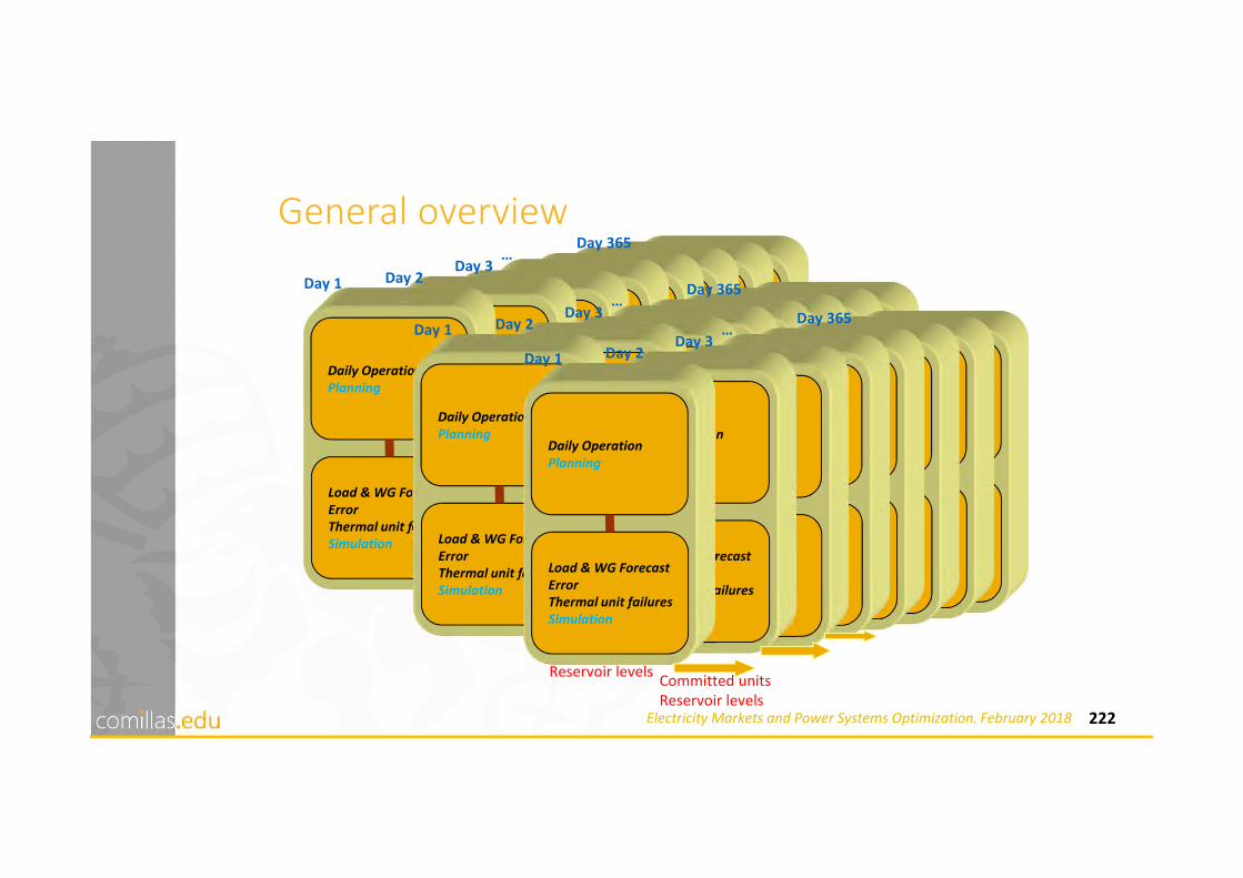
222Electricity Markets and Power Systems Optimization. February 2018
General overview
Daily Operation
Planning
WG Forecast
Error
Simulation
Daily Operation
Planning
WG Forecast
Error
Simulation
Daily Operation
Planning
WG Forecast
Error
Simulation
Daily Operation
Planning
WG Forecast
Error
Simulation
Daily Operation
Planning
WG Forecast
Error
Simulation
Daily Operation
Planning
WG Forecast
Error
Simulation
Daily Operation
Planning
WG Forecast
Error
Simulation
Daily Operation
Planning
Load & WG Forecast
Error
Thermal unit failures
Simulation
Day 1 Day 2Day 3
Day 365…
Committed units
Reservoir levels
Daily Operation
Planning
WG Forecast
Error
Simulation
Daily Operation
Planning
WG Forecast
Error
Simulation
Daily Operation
Planning
WG Forecast
Error
Simulation
Daily Operation
Planning
WG Forecast
Error
Simulation
Daily Operation
Planning
WG Forecast
Error
Simulation
Daily Operation
Planning
WG Forecast
Error
Simulation
Daily Operation
Planning
WG Forecast
Error
Simulation
Daily Operation
Planning
Load & WG Forecast
Error
Thermal unit failures
Simulation
Day 1 Day 2Day 3
Day 365…
Committed units
Reservoir levels
Daily Operation
Planning
WG Forecast
Error
Simulation
Daily Operation
Planning
WG Forecast
Error
Simulation
Daily Operation
Planning
WG Forecast
Error
Simulation
Daily Operation
Planning
WG Forecast
Error
Simulation
Daily Operation
Planning
WG Forecast
Error
Simulation
Daily Operation
Planning
WG Forecast
Error
Simulation
Daily Operation
Planning
Load & WG Forecast
Error
Thermal unit failures
Simulation
Daily Operation
Planning
Load & WG Forecast
Error
Thermal unit failures
Simulation
Day 1 Day 2Day 3
Day 365…
Committed units
Reservoir levels

223Electricity Markets and Power Systems Optimization. February 2018
Time division• Scope
• 1 year
• Period• 1 day (consecutive chronological operation)
• Subperiod• 1 hour
Day 1 Day 365
Hour 1 Hour 24
… …

224Electricity Markets and Power Systems Optimization. February 2018
Prof. Andres Ramos
https://www.iit.comillas.edu/aramos/
Thank you for your attentionThank you for your attention