THEORY OF PORTFOLIO OPTIMIZATIONIN MARKETS WITH FRICTIONS �Jak�sa Cvitani�cUSC, Department of Mathematics1042 W, 36 Pl, DRB 155Los Angeles, CA 90089cvitanic@hto.usc.eduSeptember 24, 1999AbstractThis is a survey paper on portfolio optimization problems in con-tinuous time market models. The tools of convex duality and martin-gales are used to solve these problems in the complete market case, aswell as the markets which are incomplete, due to portfolio constraintsor other market frictions such as di�erent interest rates for borrowingand lending, or presence of transaction costs. Also presented is theproblem of �nding the minimal cost of superreplicating a given claimin such markets.�Research supported in part by the National Science Foundation Grant DMS-97-32810.1

||||||||-1 IntroductionThe main topic of this survey is the problem of utility maximization fromterminal wealth for a single agent in various �nancial markets. Namely, givenagent's utility function U(�) and initial capital x > 0, he is trying to max-imize expected utility E[U(Xx;�(T ))] from his \terminal wealth", over all\admissible" portfolio strategies �(�). The same mathematical techniquesthat we employ here can be used to get similar results for maximizing ex-pected utility from consumption; we refer the interested reader to the richliterature on that problem, some of which is cited below.The seminal papers on these problems in the continuous-time completemarket model are Merton (1969, 1971). Using Ito calculus and stochasticcontrol/partial di�erential equations approach, Merton �nds a solution tothe problem in the Markovian model driven by Brownian motion process,for logarithmic and power utility functions. A comprehensive survey of hiswork is Merton (1990). For non-Markovian models one cannot deal with theproblem using partial di�erential equations. Instead, a martingale approachusing convex duality has been developed, with remarkable success in solv-ing portfolio optimization problems in diverse frameworks. The approach isparticularly well suited for incomplete markets (in which not all contingentclaims can be perfectly replicated). It consists of solving an appropriate dualproblem over a set of \state-price densities" corresponding to \shadow mar-kets" associated with the incompleteness of the original market. Given theoptimal solution Z to the dual problem, it is usually possible to show thatthe optimal terminal wealth for the primal problem is represented as the in-2

verse of \marginal utility" (the derivative of the utility function) evaluatedat Z. Early work in this spirit includes Foldes (1978a,b) and Bismut (1975),based on his stochastic duality theory Bismut (1973). The �rst paper using(implicitly) the technique in its modern form, in the complete market, isPliska (1986), followed by Karatzas, Lehoczky and Shreve (1987) and Coxand Huang (1989, 1991). The explicit use of the duality method, and inincomplete and/or constrained market models, was applied by Xu (1990),He and Pearson (1991), Xu and Shreve (1992), Karatzas, Lehoczky, Shreveand Xu (1991), Cvitani�c and Karatzas (1992, 1993), El Karoui and Quenez(1995), Jouini and Kallal (1995a), Karatzas and Kou (1996), Broadie, Cvi-tani�c and Soner (1998). An excellent exposition of these methods can befound in Karatzas and Shreve (1998), and that of discrete-time models inPliska (1997); see also Korn (1997). A de�nite treatment in a very gen-eral semimartingale framework is provided in Kramkov and Schachermayer(1998).A similar approach works in models in which the drift of the wealthprocess of the agent is concave in his portfolio strategy �(�). This includesmodels with di�erent borrowing and lending rates as well as some \largeinvestor" models. Analytical approach is used in Fleming and Zariphopulou(1991), Bergman (1995), while the tools of duality are essential in El Karoui,Peng and Quenez (1997), Cvitani�c (1997), Cuoco and Cvitani�c (1998).Portfolio optimization problems under transaction costs, usually on in-�nite horizon T = 1, have been studied mostly in Markovian models, us-ing PDE/variational inequalities methods. The literature includes Magilland Constantinides (1976), Constantinides (1979), Taksar, Klass and Assaf(1988), Davis & Norman (1990), Zariphopoulou (1992), Shreve and Soner(1994), Morton and Pliska (1995). We follow the martingale/duality ap-proach of Cvitani�c and Karatzas (1996) and Cvitani�c and Wang (1999), onthe �nite horizon T <1. While this method is powerful enough to guaran-tee existence and a characterization of the optimal solution, algorithms foractually �nding the optimal strategy are still lacking.3

In order to apply the martingale approach to portfolio optimization, we�rst have to resolve the problem of (super)replication of contingent claimsin a given market. After presenting the continuous-time complete marketmodel and recalling the classical Black-Scholes-Merton pricing in Sections 2and 3, we �nd the minimal cost of superreplicating a given claim B underconvex constraints on the proportions of wealth the agent invests in stocks,in Sections 4 and 5 (for much more general results of this kind see F�ollmerand Kramkov 1997). In the complete market this cost of superreplicationof B is equal to the Black-Scholes price of B, namely equal to the expectedvalue of B (discounted), under a change of probability measure that makesthe discounted prices of stocks martingales.In the case of a constrained market, in which the agent's hedging port-folio has to take values in a given closed convex set K, it is shown that theminimal cost of superreplication is now a supremum of Black-Scholes prices,taken over a family of auxiliary markets, parametrized by processes �(�),taking values in the domain of the support function of the set �K. Thesemarkets are chosen so that the wealth process becomes a supermartingale,under the appropriate change of measure. In the constant market param-eters framework, the minimal cost for superreplicating B under constraintscan be calculated as the Black-Scholes (unconstrained) price of an appro-priately modi�ed contingent claim B � B, and the hedging portfolio for Bautomatically satis�es the constraints.In Section 6 we show how the same methodology can be used to getanalogous results in a market in which the drift of the wealth process is aconcave function of the portfolio process.Section 7 introduces the concept of utility functions, and Section 8 provesexistence of an optimal constrained portfolio strategy for maximizing ex-pected utility from terminal wealth. This is done indirectly, by �rst solving adual problem, which is, loosely speaking, a problem to �nd an optimal changeof probability measure associated to the constrained market. The optimalportfolio policy is the one that replicates the inverse of marginal utility, eval-4

uated at the Radon-Nikodym derivative corresponding to the optimal changeof measure in the dual problem. Explicit solutions are provided in Section9, for the case of logarithmic and power utilities. Next, in Section 10 we ar-gue that it makes sense to price contingent claims in the constrained marketby calculating the Black-Scholes price in the unconstrained auxiliary marketthat corresponds to the optimal dual change of measure. Although in generalthis price depends on the utility of the agent and his initial capital, in manycases it does not. In particular, if the contraints are given by a cone, and themarket parameters are constant, the optimal dual process is independent ofutility and initial capital. This approach to pricing in incomplete marketswas suggested in Davis (1997) and further developed in Karatzas and Kou(1996).In Sections 11-14 we study the superreplication and utility maximizationproblems in the presence of proportional transaction costs. Similarly as in thecase of constraints, we identify the family of (pairs of) changes of probabilitymeasure, under which the \wealth process" is a supermartingale, and thesupremum over which gives the minimal superreplication cost of a claim inthis market. Representations of this type were obtained in various models inJouini and Kallal (1995b), Kusuoka (1995), Kabanov (1999). (It is knownthat in standard di�usion models this cost is simply the cost of the leastexpensive static (buy-and-hold) strategy which superreplicates the claim.For the case of the European call it is then equal to the price of one shareof the underlying, the result which was conjectured by Davis and Clarke(1994) and proved by Soner, Shreve and Cvitani�c (1995). The same resultwas shown to hold for more general models and claims in Leventhal andSkorohod (1997) and Cvitani�c, Pham and Touzi (1998).) Next, we considerthe utility maximization problem under transaction costs, and its dual. Thenature of the optimal terminal wealth in the primal problem is shown tobe the same as in the case of constraints - it is equal to the inverse of themarginal utility evaluated at the optimal dual solution. This result is usedto get su�cient conditions for the optimal policy to be the one of no trade5

at all - this is the case if the return rate of the stock is not very di�erentfrom the interest rate of the bank account and the transaction costs are largerelative to the time horizon.The important topic which is not considered here is approximate hedg-ing and pricing under transaction costs. Articles dealing with this prob-lem in continuous-time include Leland (1985) Avellaneda and Par�as (1993),Davis, Panas and Zariphopoulou (1993), Davis and Panas (1994), Davisand Zariphopoulou (1995), Barles and Soner (1998), Constantinides and Za-riphopoulou (1999). Other related works on the the subject of transactioncosts, that the reader may �nd useful to consult are: Bensaid, Lesne, Pag�es& Scheinkman (1992), Boyle & Vorst (1992), Edirisinghe, Naik & Uppal(1993), Flesaker & Hughston (1994), Gilster & Lee (1984), Grannan andSwindle (1996), Hodges & Neuberger (1989), Hoggard, Whalley & Wilmott(1993), Merton (1989), Morton & Pliska (1993).2 The Complete Market ModelWe introduce here the standard, Ito processes model for a �nancial marketM. It consists of one bank account and d stocks. Price processes S0(�) andS1(�); : : : ; Sd(�) of these instruments are modeled by the equationsdS0(t) = S0(t)r(t)dt ; S0(0) = 1dSi(t) = Si(t)24bi(t)dt+ dXj=1 �ij(t)dW j(t)35 ; Si(0) = si > 0 ; (2.1)for i = 1; : : : ; d, on some given time horizon [0; T ], 0 < T < 1. HereW (�) = (W 1(�); : : : ;W d(�))0 is a standard d�dimensional Brownian motionon a complete probability space (;F ; P ), endowed with a �ltration F =fFtg0�t�T , the P -augmentation of FW (t) := �(W (s); 0 � s � t) ; 0 � t �T , the �ltration generated by the Brownian motion W (�). The coe�cientsr(�) (interest rate), b(�) = (b1(�); : : : ; bd(�))0 (vector of stock return rates) and6

�(�) = f�ij(�)g1�i;j�d (matrix of stock-volatilities) of the model M, are allassumed to be progressively measurable with respect to F. Furthermore,the matrix �(�) is assumed to be invertible, and all processes r(�), b(�), �(�),��1(�) are assumed to be bounded, uniformly in (t; !) 2 [0; T ]�:The \risk premium" process�0(t) := ��1(t)[b(t)� r(t)1] ; 0 � t � T (2.2)where 1 = (1; : : : ; 1)0 2 Rd, is then bounded and F�progressively measurable.Therefore, the processZ0(t) := exp �� Z t0 �00(s)dW0(s)� 12 Z t0 jj�0(s)jj2ds� ; 0 � t � T (2.3)is a P�martingale, andP0(�) := E[Z0(T )1�]; � 2 FT (2.4)is a probability measure equivalent to P on FT . Under this risk-neutralequivalent martingale measure P0, the discounted stock prices S1(�)S0(�); : : : ; Sd(�)S0(�)become martingales, and the processW0(t) := W (t) + Z t0 �0(s)ds ; 0 � t � T ; (2.5)becomes Brownian motion, by the Girsanov theorem.We also introduce the discount process 0(t) := e�R t0 r(u)du; 0 � t � T: (2.6)and \state price density" processH0(t) := 0(t)Z0(t); 0 � t � T: (2.7)Consider now a �nancial agent whose actions cannot a�ect market prices,and who can decide, at any time t 2 [0; T ], what proportion �i(t) of his(nonnegative) wealth X(t) to invest in the ith stock (1 � i � d). Of course7

these decisions can only be based on the current information Ft, without an-ticipation of the future. With �(t) = (�1(t); : : : ; �d(t))0 chosen, the amountX(t)[1 �Pdi=1 �i(t)] is invested in the bank. Thus, in light of the dynam-ics (2.1), the wealth process X(�) � Xx;�;c(�) satis�es the linear stochasticdi�erential equationdX(t) = �dc(t) + "X(t)(1 � dXi=1 �i(t))# r(t)dt+ dXi=1 �i(t)X(t)24bi(t)dt+ dXj=1 �ij(t)dW j(t)35= �dc(t) + r(t)X(t)dt+ �0(t)�(t)X(t)dW0(t) ; X(0) = x :where the real number x > 0 represents initial capital and c(�) � 0 denotesthe agent's cumulative consumption process.We formalize the above discussion as follows.De�nition 2.1 (i) A portfolio process � : [0; T ]�! Rd is F�progressivelymeasurable and satis�es R T0 jjX(t)�(t)jj2dt <1, almost surely (here,X is thecorresponding wealth process de�ned below). A consumption process c(�) isa nonnegative, nondecreasing, progressively measurable process with RCLLpaths, with c(0) = 0 and c(T ) <1.(ii) For a given portfolio and consumption processes �(�), c(�), the pro-cess X(�) � Xx;�;c(�) de�ned by (2.9) below, is called the wealth processcorresponding to strategy (�; c) and initial capital x.(iii) A portfolio-consumption process pair (�(�); c(�)) is called admissiblefor the initial capital x, and we write (�; c) 2 A0(x), ifXx;�;c(t) � 0; 0 � t � T (2.8)holds almost surely.For the discounted version of process X(�), we get the equationd( 0(t)X(t)) = � 0(t)dc(t) + �0(t)�(t) 0(t)X(t)dW0(t): (2.9)It follows that 0(�)X(�) is a nonnegative local P0�supermartingale, hencealso a P0�supermartingale, by Fatou's lemma. Therefore, if �0 is de�ned8

to be the �rst time it hits zero, we have X(t) = 0 for t � �0, so that theportfolio values �(t) are irrelevant after that happens. Accordingly, we canand do set �(t) � 0 for t � �0. The supermartingale property impliesE0[ 0(T )Xx;�;c(T )] � x; 8 � 2 A0(x) : (2.10)Here, E0 denotes the expectation operator under the measure P0.We say that a strategy (�(�); c(�)) results in arbitrage if with the initialinvestmentx = 0 we haveX0;�;c(T ) � 0 almost surely, butX0;�;c(T ) > 0 withpositive probability. Notice that inequality (2.10) implies that an admissiblestrategy (�(�); c(�)) 2 A0(0) cannot result in arbitrage.3 Pricing in the complete marketLet us suppose now that the agent promises to pay a random amount B(!) �0 at time t = T and that he wants to invest x dollars in the market in sucha way that his pro�t \hedges away" all the risk, namely that Xx;�;c(T ) � B,almost surely. What is the smallest value of x > 0 for which such \hedging"is possible? This smallest value will then be the \price" of the contingentclaim B at time t = 0.We say that B is a contingent claim if it is a nonnegative, FT -measurablerandom variable such that 0 < E0[ 0(T )B] <1: The super-replication priceof this contingent claim is de�ned byh(0) := inffx > 0; 9(�; c) 2 A0(x) s:t: Xx;�;c(T ) � B a:s:g: (3.1)The following classical result identi�es h(0) as the expectation, under therisk-neutral probability measure, of the claim's discounted value; see Harrison& Kreps (1979), Harrison & Pliska (1981, 83).Proposition 3.1 The in�mum in (3.1) is attained, and we haveh(0) = E0[ 0(T )B] : (3.2)9

Furthermore, there exists a portfolio �B(�) such that XB(�) � Xh(0);�B;o(�) isgiven by XB(t) = 1 0(t)E0[ 0(T )BjFt] ; 0 � t � T : (3.3)Proof: Suppose Xx;�;c(T ) � B holds a.s. for some x 2 (0;1) and a suitable(�; c) 2 A0(x). Then from (2.10) we have x � z := E0[ 0(T )B] and thush(0) � z.On the other hand, from the martingale representation theorem, the pro-cess XB(t) := 1 0(t)E0[ 0(T )BjFt] ; 0 � t � Tcan be represented asXB(t) = 1 0(t)[z + Z t0 0(s)dW0(s)]for a suitable fFtg-progressively measurable process (�) with values in Rdand R T0 jj (t)jj2dt < 1, a.s. Then �B(t) := 1 0(t)XB(t)(�0(t))�1 (t) is a wellde�ned portfolio process, and we have XB(�) � Xz;�B ;0(�), by comparisonwith (2.9). Therefore, z � h(0). �Notice that Xh(0);�B ;0B (T ) = B ;almost surely. We express this by saying that contingent claimB is attainable,with initial capital h(0) and portfolio �B. In this complete market model, wecall h(0) the Black-Scholes price of B and �B(�) the Black-Scholes hedgingportfolio.Example 3.1 Constant r(�) � r > 0; �(�) � � nonsingular. In this case, thesolution S(t) = (S1(t); : : : ; Sd(t))0 is given by Si(t) = fi(t�s; S(s); �(W0(t)�W0(s))); 0 � s � t where f : [0;1)� Rd+� Rd! Rd+ is the function de�nedby fi(t; s; y; r) := si exp[(r � 12aii)t+ yi] ; i = 1; : : : ; d10

where a = ��0.Consider now a contingent claim of the type B = '(S(T )), where ' :Rd+! [0;1) is a given continuous function, that satis�es polynomial growthconditions in both jjsjj and 1=jjsjj. Then the value process of this claim isgiven byXB(t) = e�r(T�t)E0['(S(T ))jFt]= e�r(T�t) ZRd'(f(T � t; S(t); �z)) 1(2�(T � t))d=2 expf� kzk22(T � t)gdz= V (T � t; S(t));whereV (t; p) := ( e�rt RRd '(h(t; s; �z; r)) e�jjzjj2=2t(2�t)d=2 dz ; t > 0; s 2 Rd+'(s) ; t = 0; s 2 Rd+) :In particular, the price h(0) of the claim B is given, in terms of the functionV , by h(0) = XB(0) = V (T; S(0)) :Moreover, function V is the unique solution to the Cauchy problem (byFeynman-Kac theorem)12 dXi=1 dXj=1 aijxixj @2V@xi@xj + dXi=1 r(xi @V@xi � V ) = @V@t ;with the initial condition V (0; x) = '(x). Applying Ito's rule, we obtaindV (T � t; S(t)) = rV (T � t; S(t)) + dXi=1 dXj=1 �ijSi(t) @S@xi (T � t; Si(t))dW (j)0 (t):Comparing this with (2.9), we get that the hedging portfolio is given by�i(t)V (T � t; S(t)) = Si(t)@V@xi (T � t; S(t)); i = 1; : : : ; d:It should be noted that none of the above depends on vector b(�) of returnrates. 11

If, for example, we have d = 1 and in the case '(s) = (s � k)+ ofa European call option, with � = �11 > 0, exercise price k > 0; N(z) =1p2� R z�1 e�u2=2du and d�(t; s) := 1�pthlog( sk )+ (r� �22 )ti, we have the famousBlack & Scholes (1973) formulaV (t; s) = ( sN(d+(t; s))� ke�rtN(d�(t; s)) ; t > 0; s 2 (0;1)(s� k)+ ; t = 0; s 2 (0;1)) :4 Portfolio ConstraintsWe �x throughout a nonempty, closed, convex set K in Rd, and denoteby �(x) := sup�2Kf��0xg (4.1)the support function of the set �K. This is a closed, positively homogeneous,proper convex function on Rd (Rockafellar (1970), p.114). It is �nite on itse�ective domain ~K := fx 2 Rd = �(x) <1g (4.2)which is a convex cone (called the \barrier cone" of �K). For the rest of thepaper we assume the following mild conditions.Assumption 4.1 The closed convex set K � Rd contains the origin; inother words, the agent is allowed not to invest in stocks at all. In particular,�(�) � 0 on ~K. Moreover, the set K is such that �(�) is continuous on thebarrier cone ~K of (4.2).The role of the closed, convex set K that we just introduced, is to modelreasonable constraints on portfolio choice. One may, for instance, considerthe following examples.(i) Unconstrained case: K = Rd. Then ~K = f0g, and � � 0 on ~K.(ii) Prohibition of short-selling: K = [0;1)d. Then ~K = K, and � � 0on ~K. 12

(iii) Incomplete Market: K = f� 2 Rd;�i = 0; 8 i = m + 1; : : : ; dg forsome �xed m 2 f1; : : : ; d � 1g: Then ~K = fx 2 Rd; xi = 0; 8 i = 1; : : : ;mgand � � 0 on ~K.(iv) K is a closed, convex cone in Rd. Then ~K = fx 2 Rd; �0x � 0; 8 � 2Kg is the polar cone of �K, and � � 0 on ~K . This case obviouslygeneralizes (i) - (iii).(v) Prohibition of borrowing: K = f� 2 Rd;Pdi=1 �i � 1g. Then ~K =fx 2 Rd; x1 = : : : = xd � 0g, and �(x) = �x1 on ~K.(vi) Rectangular constraints: K = �di=1Ii; Ii = [�i; �i] for some �xednumbers �1 � �i � 0 � �i � 1, with the understanding that the intervalIi is open to the right (left) if bi = 1 (respectively, if �i = �1). Then�(x) = Pdi=1(�ix�i � �ix+i ) and ~K = Rd if all the �;is; � ;is are real. Ingeneral, ~K = fx 2 Rd;xi � 0; 8 i 2 S+ and xj � 0; 8 j 2 S�g whereS+ := fi = 1; : : : ; d = �i =1g; S� := fi = 1; : : : ; d = �i = �1g . �We consider now only portfolios that take values in the given, convex,closed set K � Rd, i.e., we replace the set of admissible policies A0(x) withA0(x) := f(�; c) 2 A0(x); �(t; !) 2 K for ` �P� a:e: (t; !)g :Here, ` stands for Lebesgue measure on [0; T ].Denote by D the set of all bounded progressively measurable process �(�)taking values in ~K a.e. on � [0; T ]. In analogy with (2.2)-(2.5), introduce��(t) := ��1(t)[�(t) + b(t)� r(t)1] ; 0 � t � T; (4.3)Z�(t) := exp �� Z t0 �0�(s)dW (s) � 12 Z t0 jj��(s)jj2ds� ; 0 � t � T; (4.4)P�(�) := E[Z�(T )1�]; � 2 FT (4.5)W�(t) := W (t) + Z t0 ��(s)ds ; 0 � t � T; (4.6)a P ��Brownian motion. Also denote �(t) := e�R t0 [r(u)+�(�(u))]du (4.7)13

and H�(t) := �(t)Z�(t): (4.8)Proposition 4.1 The (nonnegative) processM�(t) := H�(t)X(t) + Z t0 H�(s) [X(s)(�(�s) + � 0(s)�(s))ds+ dc(s)]is a P� supermartingale for every � 2 D and (�; c) 2 A0(x). In particular,sup�2DE "H�(T )X(T ) + Z T0 H�(s)X(s)f�(�s) + �0(s)�(s)gds# � x : (4.9)Proof: Ito's rule impliesM�(t) = x+ Z t0 H�(s)X(s) [�0(s)�(s)� �0�(s)] dW (s):In particular, the process on the right-hand side is a nonnegative local mar-tingale, hence a supermartingale. �In general, there are several interpretations for the processes � 2 D:they are stochastic \Lagrange multipliers" associated with the portfolio con-straints; in economics jargon, they correspond to the shadow prices relevantto the incompletness of the market introduced by constraints. The numberh�(0) := E� [ �(T )B] = E[H�(T )B] is the unconstrained hedging price for Bin an auxiliary marketM� ; this market consists of a bank account with inter-est rate r(�)(t) := r(t)+ �(�(t)) and d stocks, with the same volatility matrixf�ij(t)g1�i;j�d as before and return rates b(�)i (t) := bi(t)+�i(t)+ �(�(t)); 1 �i � d; for any given � 2 D. We shall show that the price for superreplicatingB with a constrained portfolio in the market M, is given by the supre-mum of the unconstrained hedging prices h�(0) in these auxiliary marketsM�; � 2 D.5 Superreplication under portfolio constraintsConsider the minimal cost of superreplication of the claim B in the marketwith constraints: 14

(6:1) h(0) := ( inffx > 0;9(�; c) 2 A0(x); s:t: Xx;�;c(T ) � B a:s:g1 , if the above set is empty ) :Let us denote by S the set of all fFtg-stopping times � with values in[0; T ], and by S�;� the subset of S consisting of stopping times � s.t. � � � ��, for any two � 2 S; � 2 S such that � � �, a.s. For every � 2 S consideralso the F� -measurable random variableV (� ) := ess sup�2D E�[B 0(T ) expf� Z T� �(�(s))dsgjF� ]: (5.1)We will show that h(0) = V (0). We �rst needProposition 5.1 If V (0) = sup�2D E�[ �(T )B] < 1, then the family ofrandom variables fV (� )g�2S satis�es the equation of Dynamic ProgrammingV (� ) = ess sup�2D�;� E� [V (�) expf� Z �� �(�(u))dugjF�] ; 8 � 2 S�;T ; (5.2)where D�;� is the restriction of D to the stochastic interval [[�; �]].Proposition 5.2 The process V = fV (t);Ft; 0 � t � Tg can be consideredin its RCLL modi�cation and, for every � 2 D,8>><>>: Q�(t) := V (t)e�R t0 �(�(u))du;Ft; 0 � t � Tis a P�-supermartingale with RCLL paths9>>=>>; : (5.3)Furthermore, V is the smallest adapted, RCLL process that satis�es (5.3) aswell as V (T ) = B 0(T ); a:s: (5.4)Proof of Proposition 5.1: Let us start by observing that, for any � 2 S;the random variableJ�(�) := E� [V (T )e�R T� �(�(s))dsjF�]15

= E[Z�(�)Z�(�; T )V (T )e�R T� �(�(s))dsjF�]E[Z�(�)Z�(�; T )jF�]= E[Z�(�; T )V (T )e�R T� �(�(s))dsjF�]depends only on the restriction of � to [[�; T ]] (we have used the notationZ�(�; T ) = Z�(T )Z�(�) ). It is also easy to check that the family of random variablesfJ�(�)g�2D is directed upwards; indeed, for any � 2 D; � 2 D and withA = f(t; !); J�(t; !) � J�(t; !)g the process � := �1A + �1Ac belongs to Dand we have a.s. J�(�) = maxfJ�(�); J�(�)g; then from Neveu (1975), p.121,there exists a sequence f�kgk2N � D such that fJ�k(�)gk2N is increasing and(i) V (�) = limk!1 " J�k (�); a:s:Returning to the proof itself, let us observe thatV (� ) = esssup�2D�;T E� [e�R �� �(�(s))dsE�fV (T )e�R T� �(�(s))dsjF�gjF� ]� esssup�2D�;T E� [e�R �� �(�(s))dsV (�)jF� ]; a:s:To establish the opposite inequality, it certainly su�ces to pick � 2 D andshow that(ii) V (� ) � E�[V (�)e�R �� �(�(s))dsjF� ]holds almost surely.Let us denote byM�;� the class of processes � 2 D which agree with � on[[�; �]]. We haveV (� ) � ess sup�2M�;� E�[e� R �� �(�(s))ds�R T� �(�(s))dsV (T )jF�]= ess sup�2M�;� E�[e� R �� �(�(s))dsE�fe�R T� �(�(s))dsV (T )jF�gjF� ]:Thus, for every � 2M�;�, we haveV (� ) � E� [e�R �� �(�(s))dsJ�(�)jF� ]16

= E[Z�(� )Z�(�; �)EfZ�(�; T )jF�ge� R �� �(�(s))dsJ�(�)jF� ]E[Z�(� )Z�(�; �)EfZ�(�; T )jF�gjF� ]= E[Z�(�; �)e�R �� �(�(s))dsJ�(�)jF� ]= E[Z�(�; �)e�R �� �(�(s))dsJ�(�)jF� ]= : : : = E�[e�R �� �(�(s))dsJ�(�)jF� ]:Now clearly we may take f�kgk�N �M�;� in (i), as J�(�) depends only on therestriction of � on [[�; T ]]; and from the above,V (� ) � limk!1 " E�[e�R �� �(�(s))dsJ�k(�)jF� ]= E�[e�R �� �(�(s))ds limk!1 " J�k(�)jF� ]= E�[e�R �� �(�(s))dsV (�)jF� ]; a:s:by Monotone Convergence. �It is an immediate consequence of this proposition that(iii) V (� )e� R �0 �(�(u))du � E� [V (�)e�R �0 �(�(u))dujF� ]; a:s:holds for any given � 2 S; � 2 S�;T and � 2 D.Proof of Proposition 5.2: Let us consider the positive, adapted processfV (t; !);Ft; t 2 [0; T ] \Qg for ! 2 . From (iii), the processfV (t; !)e� R t0 �(�(s;!))ds; Ft; t 2 [0; T ]\ Qg for ! 2 is a P� - supermartingale on [0; T ]\Q, whereQ is the set of rational numbers,and thus has a.s. �nite limits from the right and from the left (recall Propo-sition 1.3.14 in Karatzas & Shreve (1991), as well as the right-continuity ofthe �ltration fFtg). Therefore,V (t+; !) := ( lim s#ts2Q V (s; !) ; 0 � t < TV (T; !) ; t = T )V (t�; !) := ( lim s"ts2Q V (s; !) ; 0 < t � TV (0) ; t = 0 )17

are well-de�ned and �nite for every ! 2 �; P (�) = 1; and the resultingprocesses are adapted. Furthermore (loc.cit.), fV (t+)e�R t0 �(�(s))ds; Ft; 0 �t � Tg is a RCLL, P� -supermartingale, for all � 2 D; in particular,V (t+) � E�[V (T )e�R Tt �(�(s))dsjFt]; a:s:holds for every � 2 D, whence V (t+) � V (t) a.s. On the other hand, fromFatou's lemma we have for any � 2 D:V (t+) = E� [ limn!1 V (t+ 1n) e� R t+1=nt �(�(u))dujFt]� limn!1E� [V (t+ 1n) e� R t+1=nt �(�(u))dujFt] � V (t); a:s:and thus fV (t+); Ft; 0 � t � Tg; fV (t); Ft; 0 � t � Tg are modi�cationsof one another.The remaining claims are immediate. �Theorem 5.1 For an arbitrary contingent claim B, we have h(0) = V (0).Furthermore, if V (0) < 1, there exists a pair (�; c) 2 A0(V (0)) such thatXV (0);�;c(T ) = B; a:s:Proof: Proposition 4.1 implies x � E�[ �(T )B] for every � 2 D, henceh(0) � V (0).We now show the more di�cult part: h(0) � V (0). Clearly, we mayassume V (0) < 1. From (5.3), the martingale representation theorem andthe Doob-Meyer decomposition, we have for every � 2 D:Q�(t) = V (0) + Z t0 0�(s)dW�(s)�A�(t); 0 � t � T ; (5.5)where �(�) is an Rd-valued, fFtg-progressively measurable and a.s. square-integrable process and A�(�) is adapted with increasing, RCLL paths andA�(0) = 0; EA�(T ) < 1 a.s. The idea then is to consider the positive,adapted, RCLL processX(t) := V (t) 0(t) = Q�(t) �(t) ; 0 � t � T (8 � 2 D) (5.6)18

with X(0) = V (0); X(T ) = B a.s., and to �nd a pair (�; c) 2 A0(V (0)) suchthat X(�) = XV (0);�;c(�). This will prove that h(0) � V (0).In order to do this, let us observe that for any � 2 D; � 2 D we havefrom (5.3) Q�(t) = Q�(t) exp �Z t0 f�(�(s))� �(�(s))gds� ;and from (5.5):dQ�(t) = exp[R t0f�(�(s))� �(�(s))gds] � [Q�(t)f�(�(t))� �(�(t))gdt+ 0�(t)dW�(t)� dA�(t)] (5.7)= exp[R t0f�(�(s))� �(�(s))gds] � [X(t) �(t)f�(�(t))� �(�(t))gdt�dA�(t) + 0�(t)��1(t)(�(t)� �(t))dt+ 0�(t)dW�(t)] :Comparing this decomposition withdQ�(t) = 0�(t)dW�(t)� dA�(t) ; (5.8)we conclude that 0�(t) eR t0 �(�(s))ds = 0�(t) eR t0 �(�(s))dsand hence that this expression is independent of � 2 D: 0�(t) eR t0 �(�(s))ds = X(t) 0(t)�0(t)�(t); 8 0 � t � T; � 2 D (5.9)for some adapted, Rd-valued, a.s. square integrable process � (we do notknow yet that � takes values in K). If X(t) = 0, then X(s) = 0 for all s � t,and we can set, for example, �(s) = 0, s � t (in fact, one can show thatR T0 1fX(t)=0gk �(t)k2dt = 0, a.s; see Karatzas and Kou (1996)).Similarly, we conclude from (5.7), (5.9) and (5.8):eR t0 �(�(s))dsdA�(t)� 0(t)X(t)[�(�(t)) + �0(t)�(t)]dt= eR t0 �(�(s))dsdA�(t)� 0(t)X(t)[�(�(t)) + �0(t)�(t)]dt19

and hence this expression is also independent of � 2 D:c(t) := Z t0 �1� (s)dA�(s)� Z t0 X(s)[�(�(s)) + � 0(s)�(s)]ds ; (5.10)for every 0 � t � T; � 2 D. Setting � � 0, we obtain c(t) = R t0 �10 (s)dA0(s); 0 �t � T and hence( c(�) is an increasing, adapted, RCLL processwith c(0) = 0 and c(T ) <1; a:s: ) : (5.11)Next, we claim that�(�) + � 0�(t; !) � 0; ` P� a:e: (5.12)holds for every � 2 ~K. Then Theorem 13.1 of Rockafellar (1970) (togetherwith continuity of �(�) and closedness of K) leads to the fact that�(t; !) 2 K holds ` P � a:e: on [0; T ]� :In order to verify (5.12), notice that from (5.10) we obtainZ t0 �1� (s)A�(s)ds = c(t) + R t0 X(s)f�(�s) + � 0s�sgds; 0 � t � T; � 2 D:Fix � 2 ~K and de�ne the set F� := f(t; !) 2 [0; T ]�; �(�))+� 0�(t; !) < 0g.Let �(t) := [�1F c� + n�1F� ]; n 2 N; then � 2 D, and assuming that (5.12)does not hold, we get for n large enoughE[Z T0 �1� (s)A�(s)ds] = E hc(T ) + R T0 X(t)1F c� f�(�) + � 0�(t)gdti+nE hR T0 X(t)1F�f�(�) + � 0�(t)gdti < 0 ;a contradiction.Now we can put together (5.5)-(5.10) to deduced( �(t)X(t)) = dQ�(t) = 0�(t)dW�(t)� dA�(t)= �(t)[�dc(t)� X(t)f�(�(t)) + � 0(t)�(t)gdt (5.13)+X(t)�0(t)�(t)dW�(t)] ;20

for any given � 2 D. As a consequence, the processM�(t) := �(t)X(t) + Z t0 �(s)dc(s) + Z t0 �(s)X(s)[�(�(s)) + � 0(s)�(s)]ds(5.14)= V (0) + Z t0 �(s)X(s)�0(s)�(s)dW�(s) ; 0 � t � Tis a nonnegative, P� -local martingale, hence supermartingale. In particular,for � � 0, (5.13) gives:d( 0(t)X(t)) = � 0(t)dc(t) + 0(t)X(t)�0(t)�(t)dW0(t);X(0) = V (0) ; X(T ) = B ;which is equation (2.9) for the process X(�) of (5.6). This shows X(�) �XV (0);�;c(�), and hence h(0) � V (0) <1: �De�nition 5.1 We say that claim B is K�hedgeable if its minimal costof superreplication is �nite, V (0) < 1; we say it is K�attainable if thereexists a portfolio process � with values in K such that (�; 0) 2 A0(V (0)) andXV (0);�;0(T ) = B, a.s.Theorem 5.2 For a given K-hedgeable contingent claim B, and any given� 2 D, the conditionsfQ�(t) = V (t)e�R t0 �(�(u))du;Ft; 0 � t � Tg is a P�-martingale (5.15)� achieves the supremum in V (0) = sup��D E�[B �(T )] (5.16)( B is K-attainable (by a portfolio �), and thecorresponding �(�)XV (0);�;0(�) is a P�-martingale ) (5.17)are equivalent, and implyc(t; !) = 0; �(�(t; !)) + �0(t; !)�(t; !) = 0; ` P � a:e: (5.18)for the pair (�; c) 2 A0(V (0)) of Theorem 5.1.21

Proof: The P�-supermartingale Q�(�) is a P�-martingale, if and only ifQ�(0) = E�Q�(T ), V (0) = E�[B �(T )], (5.16).On the other hand, (5.15) implies A�(�) � 0, and so from (5.10): c(t) =� R t0 X(s)[�(�(s))+�0(s)�(s)]ds. Now (5.18) follows from the increase of c(�)and the nonnegativity of �(�) + �0�; since � takes values in K.From (5.16) (and its consequences (5.15), (5.18)), the process X(�) of (5.6)and (5.13) coincides with XV (0);�;0(�), and we have: X(T ) = B almost surely, �(�)X(�) is a P�-martingale; thus (5.17) is satis�ed with � � �. On theother hand, suppose that (5.17) holds; then V (0) = E�[B �(T )], so (5.16)holds.Theorem 5.3 Let B be a K-hedgeable contingent claim. Suppose that, forany � 2 D with �(�) + � 0� � 0,Q�(�) in (5.3) is of class DL[0; T ]; under P� : (5.19)Then, for any given � 2 D, the conditions (5.15), (5.16), (5.18) areequivalent, and imply( B is K-attainable (by a portfolio �), and thecorresponding 0(�)XV (0);�;0(�) is a P0-martingale ) : (5.20)Proof: We have already shown the implications (5.15) , (5.16) ) (5.18).To prove that these three conditions are actually equivalent under (5.19),suppose that (5.18) holds; then from (5.10): A�(�) � 0, whence the P�-localmartingale Q�(�) is actually a P�-martingale (from (5.5) and the assumption(5.19)); thus (5.15) is satis�ed.Clearly then, if (5.15), (5.16), (5.18) are satis�ed for some � 2 D, theyare satis�ed for � � 0 as well; and from Theorem (5.2), we know then that(5.20) (i.e., (5.17) with � � 0) holds.Remark 5.1 (i) Loosely speaking, Theorems 5.2, 5.3 say that the supremumin (5.16) is attained if and only if it is attained by � � 0, if and only if theBlack-Scholes (unconstrained) portfolio happens to satisfy constraints.22

(ii) It can be shown that the conditions V (0) <1 and (5.19) are satis�ed(the latter, in fact, for every � 2 D) in the case of the simple European calloption B = (S1(T )� k)+, providedthe function x 7! �(x) + x1 is bounded from below on ~K: (5.21)The same is true for any contingent claim B that satis�es B � �S1(T ) a.s.,for some � 2 (0;1): Note that the condition (5.21) is indeed satis�ed, ifthe convex set K contains both the origin and the point (1; 0; : : : ; 0) (andthus also the line-segment adjoining these points); for then x1 + �(x) �x1 + sup0���1(��x1) = x+1 � 0; 8x 2 ~K:We would like now to have a method for calculating the price h(0). In order todo that, we assume constant market coe�cients r; b; � and consider only theclaims of the form B = b(S(T )), for a given, lower-semicontinuous functionb. Similarly as in the no-constraints case, the minimal hedging process willbe given as X(t) = V (t; S(t)), for some function V (t; s), depending on theconstraints. Introduce also, for a given process �(�) in Rd, the auxiliary,shadow economy vector of stock prices S�(�) bydS�i (t) = S�i (t)24rdt + dXj=1�ijdW (j)� (t)35and notice that its distribution under measure P� is the same as the one ofS(�) under P0. From Theorem 5.1 we know thatV (t; s) = sup�2DE� �b(S(T ))e�R Tt (r+�(�(s)))ds ���� S(t) = s� : (5.22)We will show that this complex looking stochastic control problem has asimple solution. First, we modify the value of the claim by considering thefollowing function: b(s) = sup�2 ~K b(se��)e��(�):Here, se�� = (s1e��1 ; : : : ; sde��d)0, and we use the same notation for thecomponentwise product of two vectors throughout.23

Theorem 5.4 The minimal K-hedging price function V (t; s) of the claimb(S(T )) is the Black-Scholes cost function for replicating b(S(T )). In partic-ular, under technical assumptions, it is the solution to the PDEVt + 12 dXi=1 dXj=1 aijsisjVsisj + r dXi=1 siVsi � V ! = 0; (5.23)with the terminal conditionV (T; s) = b(s); s 2 Rd+; (5.24)and the corresponding hedging strategy � satis�es the constraints. Undertechnical assumptions, it is given by�i(t) = si(t)Vsi(t; s(t))=V (t; s(t)); i = 1; : : : ; d: (5.25)Proof: (a) We �rst show that hedging b(S(T )) under constraints is no moreexpensive than hedging b(S(T )) without constraints. Let � 2 D and observethat, from the properties of the support function and the cone property of~K, (i) ^b = b(ii) Z Tt �(�s)ds � �(Z Tt �sds);(iii) Z Tt �sds is an element of ~K;where R Tt �(s)ds := (R Tt �1(s)ds; :::; R Tt �d(s)ds)0. Moreover, we have(iv) S�i (t) = Si(t)eR t0 �i(s)ds;because the processes on the left-hand side and the right-hand side satisfythe same linear SDE. Then, for every � 2 D we haveE� [b(S(T ))e�R T0 (r+�(�(s)))ds] � E� [b(S�(T )e�R T0 �(s)ds)e��(R T0 �(s)ds)e�rT ]� E� [sup�2 ~K b(S�(T )e��)e��(�)e�rT ] (5.26)= E� [^b(S�(T ))e�rT ] = E0[b(S(T ))e�rT ]:24

Similarly for conditional expectations of (5.22), hence V (t; s) is no largerthan the Black-Scholes price process of the claim b(S(T )).(b) To conclude we have to show that to superreplicate b(S(T )) we haveto hedge at least b(S(T )). It is su�cient to prove that the left limit of V (t; s)at t = T is larger than b(s). For this, let f�kg be the maximizing sequencein the cone ~K attaining b(s), i.e., such that b(se��k)e��(�k) converges to b(s)as k goes to in�nity. Then, using (for �xed t < T ) constant deterministiccontrols �k(t) = �k=(T � t) in (5.22), we getV (t; s) � E0[b(S(T )e��k)e��(�k)e�r(T�t) j S(t) = s];hence limt!T V (t; s) � b(se��k)e��(�k)and letting k to in�nity, we �nish the proof. Here is a sketch of a PDE prooffor part (a) in the proof above: Let V be the solution to (5.23), (5.24). Fora given � 2 ~K, consider the function W� = (sVs)0� + �(�)V , where Vs isthe vector of partial derivatives of V with respect to si, i = 1; : : : ; d. ByTheorem 13.1 in Rockafellar (1970), to prove that portfolio � of (5.25) takesvalues in K, it is su�cient to prove that W� is non-negative, for all � 2 ~K.It is not di�cult to see (assuming enough smoothness) that W� solves PDE(5.23), too. Moreover, it is also possible to check that W�(s; T ) � 0. So, bythe maximum principle, W� � 0 everywhere.Example 5.2 We restrict ourselves to the case of only one stock, d = 1, andthe constraints of the type K = [�l; u]; (5.27)with 0 � l; u � +1, with the understanding that the interval K is open tothe right (left) if u = +1 (respectively, if l = +1). It is straightforward tosee that �(�) = l�+ + u��;25

and ~K = R if both l and u are �nite. In general,~K = fx 2 R : x � 0 if u = +1; x � 0 if l = +1g:For the European call b(s) = (s � k)+, one easily gets that b(s) � 1, ifu < 1, b(s) = s if u = 1 (no-borrowing) and b(s) = b(s) if u = 1 (short-selling constraints don't matter for the call option). For 1 < u <1 we have(by ordinary calculus)b(s) = ( s� k ; s � kuu�1ku�1 �(u�1)sku �u ; s < kuu�1 :For the European put b(s) = (k� s)+, one gets b = b if l =1 (borrowingconstraints don't matter), b � k if l = 0 (no short-selling), and otherwiseb(s) = ( k � s ; s � kll+1kl+1 � ku(l+1)s�l ; s > kll+1 :Numerical results on hedging these (and other) options under the aboveconstraints can be found in Broadie, Cvitani�c and Soner (1998).6 The Case of Concave DriftIn this section we consider the case of an agent whose drift is a concavefunction of his trading strategy. The most prominent example is the case inwhich the borrowing rate R is larger than the lending rate r. Moreover, italso includes examples of a \large investor" who can in uence the drift ofthe asset prices by trading in the market (see Cuoco and Cvitani�c 1998).We assume that the wealth process X(t) satis�es the stochastic di�eren-tial equationdX(t) = X(t)g(t; �t)dt+X(t)�0(t)�(t)dW (t)�dc(t) ; X(0) = x > 0; (6.1)26

where function g(t; �) is concave for all t 2 [0; T ], and uniformly (with respectto t) Lipschitz:jg(t; x)� g(t; y)j � kkx� yk; 8 t 2 [0; T ]; x; y 2 Rd;for some 0 < k <1: Moreover, we assume g(�; 0) � 0.In analogy with the case of constraints we de�ne the convex conjugatefunction ~g of g by ~g(t; �) := sup�2Rdfg(t; �) + �0�g; (6.2)on its e�ective domain Dt := f� : ~g(�; t) < 1g: Introduce also the class Dof processes �(t) taking values in Dt, for all t. It is clear that under aboveassumptions D is not empty. We also assume, for simplicity, that function~g(t; �) is bounded on its e�ective domain, uniformly in t.For a given fFtg�progressively measurable process �(�) with values in Rdwe introduce �(t; u) := expf� Z ut ~g(s; �s)dsg; �(t) := �(0; t);dZ�(t) := ���1(t)�(t)Z�(t)dW (t); Z�(0) = 1; H�(t) := Z�(t) �(t) : (6.3)For every � 2 D we have (by Ito's rule)H�(t)X(t) + Z t0 H�(s) [X(s)(~g(s; �s)� g(s; �s)� �0(s)�(s))ds + dc(s)]= x+ Z t0 H�(s)X(s) h�0(s)�(s) + ��1(s)�(s)i dW (s): (6.4)In particular, the process on the right-hand side is a nonnegative local mar-tingale, hence a supermartingale. Therefore we get the following necessarycondition for � to be admissible:sup�2D E "H�(T )X(T ) + Z T0 H�(s)X(s)f~g(s; �s)� g(s; �s)� �0(s)�(s)gds# � x :(6.5)27

The supermartingale property excludes arbitrage opportunities from thismarket: if x = 0; then necessarily X(t) = 0, 8 0 � t � T , almost surely.Next, for a given � 2 D, introduce the processW�(t) := W (t)� Z t0 ��1(s)�(s)ds ;as well as the measureP�(A) := E[Z�(T )1A] = E�[1A]; A 2 FT :It can be shown under our assumptions that the sets Dt are uniformlybounded. Therefore, if � 2 D, then Z�(�) is a martingale. Thus, for ev-ery � 2 D, the measure P� is a probability measure and the process W�(�)is a P��Brownian motion, by Girsanov theorem.Given a contingent claim B, consider, for every stopping time � , theF� -measurable random variableV (� ) := ess sup�2DE� [B �(�; T )jF�]:The proof of the following theorem is similar to the corresponding theoremin the case of constraints.Theorem 6.1 For an arbitrary contingent claim B, we have h(0) = V (0).Furthermore, there exists a pair (�; c) 2 A0(V (0)) such that XV (0);�;c(�) =V (�):The theorem gives the minimal hedging price for a claim B; in fact, itis easy to see (using the same supermartingale argument as before) that theprocess V (�) is the minimal wealth process that hedges B. There remainsthe question of whether consumption is necessary. We show that, in fact,c(�) � 0.Theorem 6.2 Every contingent claim B is attainable, namely the processc(�) from Theorem 6.1 is a zero-process.28

Proof : Let f�n;n 2 Ng be a maximizing sequence for achieving V (0), i.e.,limn!1 E�n [B �n(T )] = V (0): Similarly to (6.5), one can getsup�2D E� " �(T )V (T ) + Z T0 �(t)dc(t)# � V (0):Since V (T ) = B, this implies limn!1 E�n R T0 �n(t)dc(t) = 0 and, since theprocesses �n(�) are bounded away from zero (uniformly in n), limn!1 E[Z�n(T )c(T )] =0: Using weak compactness arguments as in Cvitani�c & Karatzas (1993, The-orem 9.1) we can show that there exists � 2 D such that limn!1 E[Z�n c(T )] =E[Z�(T )c(T )] = 0 (along a subsequence). It follows that c(�) � 0: �The theorems above also follow from the general theory of BackwardStochastic Di�erential Equations, as presented in El Karoui, Peng and Quenez(1997).Example 6.3 Di�erent borrowing and lending rates. We have studied so fara model in which one is allowed to borrow money, at an interest rate R(�)equal to the bank rate r(�). In this section we consider the more generalcase of a �nancial market M� in which R(�) � r(�); without constraints onportfolio choice. We assume that the progressively measurable process R(�)is also bounded.In this market M� it is not reasonable to borrow money and to investmoney in the bank at the same time. Therefore, we restrict ourselves topolicies for which the relative amount borrowed at time t is equal to �1 �Pdi=1 �i(t)��. Then, the wealth process X = Xx;�;c corresponding to initialcapital x > 0 and portfolio/consumption pair (�; c), satis�esdX(t) = r(t)X(t)dt� dc(t)+X(t) "�0(t)�(t)dW0(t)� (R(t)� r(t))�1 � dXi=1 �i(t)��dt# :We get ~g(�(t)) = r(t)� �1(t) for � 2 D, whereD := f �; � progressively measurable, Rd� valued process with29

r �R � �1 = : : : = �d � 0; ` P � a:e:gWe also have~g(�(t))� g(t; �(t))� �0(t)�(t) = [R(t)� r(t) + �1(t)]�1�Pdi=1 �i(t)����1(t)�1 �Pdi=1 �i(t)�+;for 0 � t � T . It can be shown, in analogy to the case of constraints, thatthe optimal dual process �(�) 2 D can be taken as the one that attains zeroin this equation, namely as�(t) = �1(t)1; �1(t) := [r(t)�R(t)] 1fPdi=1 �i(t)>1g: �Assume now constant coe�cients, and observe that the stock price pro-cesses vector satis�es the equationsdSi(t) = Si(t)[bi(t)dt+ dXi=1 �ijdW j(t)]= Si(t)[(r � �1(t))dt+ dXi=1 �ijdW j� (t)]; 1 � i � d;for every � 2 D. Consider now a contingent claim of the form B = '(S(T )),for a given continuous function ' : Rd+ ! [0;1) that satis�es a polynomialgrowth condition, as well as the value functionQ(t; s) := sup�2D E�['(S(T ))e�R Tt (r��1(s))dsjS(t) = s]on [0; T ]� Rd+. Clearly, the processes X; V are given asX(t) = Q(t; S(t)); V (t) = e�rtX(t) ; 0 � t � T;whereQ solves the semilinear parabolic partial di�erential equation of Hamilton-Jacobi-Bellman (HJB) type@Q@t + 12Xi Xj aijsisj @2Q@si@sj + maxr�R��1�0 "(r � �1)fXi si@Q@si �Qg# = 0;30

for 0 � t < T; s 2 Rd+; Q(T; s) = '(s); s 2 Rd+(see Lady�zenskaja, Solonnikov & Ural'tseva 1968 for the basic theory of suchequations, and Fleming & Rishel 1975, Fleming and Soner 1993 for the con-nections with stochastic control). The maximization in the HJB equationis achieved by ��1 = (r � R)1fPi si @Q@si�Qg; the portfolio �(�) and the process�1(�) are then given, respectively, by�i(t) = Si(t) � @@piQ(t; S(t))Q(t; S(t)) ; i = 1; : : : ; dand �1(t) = (r �R)1fPi �i(t)�1g:The HJB PDE becomes@Q@t + 12Xi Xj sisjaij @2Q@si@sj +R Xi si@Q@si �Q!+ � r Xi si@Q@si �Q!� = 0:Suppose now that the function ' satis�es Pi si @'(s)@si � '(s); 8 s 2 Rd+.Then the solution Q also satis�es this inequality:Xi si@Q(t; s)@si � Q(t; s); 0 � t � Tfor all s 2 Rd+ and is given as the solution to the Black-Scholes equation withr replaced with R@Q@t + 12Xi Xj sisjaij @2Q@si@sj +R Xi si@Q@si �Q! = 0 ; t < T ; s > 0Q(T; s) = '(s) ; s > 0In this case the seller's hedging portfolio �(�) always borrows: Pdi=1 �i(t) �1; 0 � t � T , and it was to be expected that all he has to do is use R as theinterest rate. Note, however, that this price may be too high for the buyerof the option. 31

7 Utility functionsA function U : (0;1) ! R will be called a utility function if it is strictlyincreasing, strictly concave, of class C1, and satis�esU 0(0+) := limx#0 U 0(x) =1 ; U 0(1) := limx!1U 0(x) = 0 :We shall denote by I the (continuous, strictly decreasing) inverse of thefunction U 0; this function maps (0;1) onto itself, and satis�es I(0+) =1; I(1) = 0. We also introduce the Legendre-Fenchel transform~U(y) := maxx>0 [U(x)� xy] = U(I(y))� yI(y); 0 < y <1of �U(�x); this function ~U is strictly decreasing and strictly convex, andsatis�es ~U 0(y) = �I(y); 0 < y <1;U(x) = miny>0 [ ~U(y) + xy] = ~U (U 0(x)) + xU 0(x) ; 0 < x <1 :It is now readily checked thatU(I(y)) � U(x) + y[I(y)� x]~U(U 0(x)) + x[U 0(x)� y] � ~U (y) ;are valid for all x > 0; y > 0. It is also easy to see that~U(1) = U(0+); ~U(0+) = U(1)hold; see Karatzas et al. (1991), Lemma 4.2.For some of the results that follow, we will need to impose the followingconditions on our utility functions:c 7! cU 0(c) is nondecreasing on (0;1) ; (7.1)32

for some � � (0; 1); � (1;1) we have : �U 0(x) � U 0( x); 8 x � (0;1) :(7.2)Condition (7.1) is equivalent toy 7! yI(y) is nonincreasing on (0;1) ;and implies that x 7! ~U(ex) is convex on R :(If U is of class C2, then condition (7.1) amounts to the statement that�cU 00(c)U 0(c) , the so-called \Arrow-Pratt measure of relative risk - aversion", doesnot exceed 1. For the general treatment under the weakest possible conditionson the utility function see Kramkov and Schachermayer 1998.)Similarly, condition (7.2) is equivalent to havingI(�y) � I(y); 8 y � (0;1) for some � � (0; 1); > 1 :Iterating this, we obtain the apparently stronger statement8 � � (0; 1); 9 � (1;1) such that I(�y) � I(y); 8 y � (0;1) :8 Portfolio optimization under constraintsIn this section we consider the optimization problem of maximizing utilityfrom terminal wealth for an investor subject to the portfolio constraints givenby set K , i.e., we want to maximizeJ(x;�) := EU(Xx;�(T )) ;over the class A00 of constrained portfolios � for which (�; 0) 2 A0(x) andwhich satisfy EU�(Xx;�(T )) <1:33

The value function of this problem will be denoted byV (x) := sup�2A00(x)J(x;�) ; x 2 (0;1) : (8.1)We assume that V (x) <1, 8 x 2 (0;1) : It is fairly straightforwardthat the function V (�) is increasing and concave on (0;1). and that thisassumption is satis�ed if the function U is nonnegative and satis�es thegrowth condition0 � U(x) � �(1 + x�) ; 8 x 2 (0;1) (8.2)for some constants � 2 (0;1) and � 2 (0; 1) - see Karatzas et al. (1991)for details.Recall the notation H�(t) = �(t)Z�(t)of (4.8). We introduce the functionX�(y) := EhH�(T )I(yH�(T ))i ; 0 < y <1;and the class H of ~K-valued, progressively measurable processes �(�) suchthat E R T0 k�(t)k2dt + E R T0 �(�(t))dt < 1. Consider the subclass D0 of Hgiven by D0 := f� 2 H; X�(y) <1; 8 y 2 (0;1)g :For every � 2 D0, the function X�(�) is continuous and strictly decreasing,with X�(0+) =1 and X�(1) = 0; we denote its inverse by Y�(�).Next, we prove a crucial lemma, which provides su�cient conditions foroptimality in the problem of (8.1). The duality approach of the lemma andsubsequent analysis was implicitly used in Pliska (1986), Karatzas, Lehoczky& Shreve (1987), Cox & Huang (1989) in the case of no constraints, andexplicitly in He & Pearson (1991), Karatzas et al. (1991), Xu & Shreve(1992), Cvitani�c and Karatzas (1993) for various types of constraints.34

Lemma 8.1 For any given x > 0; y > 0 and � 2 A0(x), we haveEU(Xx;�(T )) � E ~U(yH�(T )) + yx; 8 � 2 H: (8.3)In particular, if � 2 A0(x) is such that equality holds in (8.3), for some � 2 Hand y > 0, then � is optimal for our (primal) optimization problem, while �is optimal for the dual problem~V (y) := inf�2HE ~U(yH�(T )) =: inf�2H ~J(y; �): (8.4)Furthermore, equality holds in (8.3) ifXx;�(T ) = I(yH�(T )) a:s:; (8.5)�(�t) = �� 0(t)�(t) a:e:; (8.6)E[H�(T )Xx;�(T )] = x (8.7)(the latter being equivalent to � 2 D0 and y = Y�(x), if (8.5) holds).Proof: By de�nitions of ~U; � we getU(X(T )) � ~U(yH�(T )) + yH�(T )X(T ) + Z T0 H�(t)X(t)[�(�t) + � 0(t)�(t)]dt:The upper bound of (8.3) follows from Proposition 4.1 (also valid for �(�) 2H); condition (8.5) follows from the de�nition of ~U(�), conditions (8.6) and(8.7) correspond toH�(�)X(�) being a martingale, not only a supermartingale.�Remark 8.1 Lemma 8.1 suggests the following strategy for solving the op-timization problem:(i) show that the dual problem (8.4) has an optimal solution �y 2 D0 forall y > 0;(ii) using Theorem 5.1, �nd the minimal hedging price hy(0) and a cor-responding portfolio �y for hedging B�y := I(yH�y(T ));35

(iii) prove (8.6) for the pair (�y; �y);(iv) show that, for every x > 0, you can �nd y = yx > 0 such thatx = hy(0) = E[H�y(T )I(yH�y(T ))]:Then (i)-(iv) would imply that �y is the optimal portfolio process for theutility maximization problem of an investor starting with initial capital equalto x.To verify that step (i) can be accomplished, we impose the followingcondition:8 y 2 (0;1); 9 � 2 H such that ~J(y; �) := E ~U (yH�(T )) <1 (8.8)We also impose the assumptionU(0+) > �1 ; U(1) =1 : (8.9)Under the condition (8.2), the requirement (8.8) is satis�ed. Indeed, weget 0 � ~U(y) � ~�(1 + y��) ; 8 y 2 (0;1)for some ~� 2 (0;1) and � = �1�� .Even though the log function does not satisfy (8.9), we solve that casedirectly in examples below.Theorem 8.1 Assume that (7.1), (7.2), (8.8) and (8.9) are satis�ed. Thencondition (i) of Remark 8.1 is true, i.e. the dual problem admits a solutionin the set D0, for every y > 0.The fact that the dual problem admits a solution under the conditions ofTheorem 8.1 follows almost immediately (by standard weak compactnessarguments) from Proposition 8.1 below. The details, as well as a rela-tively straightforward proof of Proposition 8.1, can be found in Cvitani�c andKaratzas (1992). Denote byH0 the Hilbert space of progressively measurableprocesses � with norm [[�]] = E R T0 �2(s)ds <1.36

Proposition 8.1 Under the assumptions of Theorem 8.1, the functional~J(y; �) : H0 ! R[f+1g of (8.4) is (i) convex, (ii) coercive: lim[[�]]!1 ~J(y; �)=1, and (iii) lower-semicontinuous: for every ��H0 and f�ngn�N � H0 with[[�n � �]]! 0 as n!1, we have~J(y; �) � limn!1 ~J(y; �n) :We move now to step (ii) of Remark 8.1. We have the following usefulfact:Lemma 8.2 For every � 2 H, 0 < y <1, we haveE[H�(T )B�y] � E[H�y(T )B�y] : (8.10)In fact, (8.10) is equivalent to �y being optimal for the dual problem,but we do not need that result here; its proof is quite lengthy and technical(see Cvitani�c and Karatzas 1992, Theorem 10.1). We are going to provide asimpler proof for Lemma 8.2, but under the additional assumption thatE[H�y(T )I(yH�(T ))] <1; 8� 2 H; y > 0: (8.11)Proof of Lemma 8.2: Fix " 2 (0; 1); � 2 H and de�ne (supressing depen-dence on t)G" := (1 � ")H�y + "H� ; �" := G�1" ((1� ")H�y�y + "H��);~�" := G�1" ((1� ")H�y�(�y) + "H��(�)):Then �" 2 H, because of the convexity of ~K. Moreover, we havedG" = (� + ��1�")G"dW � ~�"G"dt;and convexity of � implies �(�") � ~�", and therefore, comparing the solutionsto the respective (linear) SDE's, we getG"(�) � H�"(�); a:s::37

Since �y is optimal and ~U is decreasing, this implies"�1 �E[ ~U(yH�y(T ))� ~U(yG"(T ))]� � 0: (8.12)Next, recall that I = � ~U 0 and denote by V" the random variable insidethe expectation operator in (8.12). Fix ! 2 , and assume, supressing thedependence on ! and T , that H� � H�y . Then "�1V" = I(F )y(H� � H�y),where yH�y � F � yH�y+"y(H��H�y): Since I is decreasing we get "�1V" �yI(yH�)(H� �H�y): We get the same result when assuming H� � H�y : Thisand assumption (8.11) imply that we can use Fatou's lemma when takingthe limit as " # 0 in (8.12), which gives us (8.10). �Now, given y > 0 and the optimal �y for the dual problem, let �y be theportfolio of Theorem 5.1 for hedging the claim B�y = I(yH�y(T )). Lemma8.2 implies that, in the notation of Section 5,hy(0) = Vy(0) = E[H�y(T )I(yH�y(T ))] = initial capital for portfolio �y;so (8.7) is satis�ed for x = hy(0): It also implies, by (5.18), that (8.6) holdsfor the pair (�y; �y): Therefore we have completed both steps (ii) and (iii).Step (iv) is a corollary of the following result.Proposition 8.2 Under the assumptions of Theorem 8.1, for any given x >0, there exists y > 0 that achieves infy>0[ ~V (y) + xy] and satis�esx = X�y(y)For the (straightforward) proof see Cvitani�c and Karatzas (1992, Propo-sition 12.2). We now put together the results of this section:Theorem 8.2 Under the assumptions of Theorem 8.1, for any given x > 0there exists an optimal portfolio process � for the utility maximization prob-lem (8.1). Process � is equal to the portfolio of Theorem 5.1 for minimalyhedging the claim I(yH�y(T )), where y is given by Proposition 8.2 and �y isthe optimal process for the dual problem (8.4).38

9 ExamplesExample 9.4 Logarithmic utility. If U(x) = log x, we have I(y) = 1y ; ~U(y) =�(1 + log y) and X�(y) = 1y ; Y�(x) = 1xand therefore, the optimal terminal wealth isX�(T ) = x 1H�(T ) (9.1)for ��H optimal. (In particular D0 = H in this case). Therefore,Eh ~U(Y�(x)H�(T ))i = �1� log 1x + E�log 1H�(T )� :ButE�log 1H�(T )� = E Z T0 hr(s) + �(�(s)) + 12 jj�(s) + ��1(s)�(s)jj2ids ;and thus the dual problem amounts to a point-wise minimization of theconvex function �(x) + 12 jj�(t) + ��1(t)xjj2 over x� ~K, for every t � [0; T ]:�(t) = argminx� ~K [ 2�(x) + jj�(t) + ��1(t)xjj2 ] :Furthermore, (9.1) givesH�(t)X�(t) = x; 0 � t � T ;and using Ito's rule to get the SDE for H�(�)X�(�) we get, by equating theintegrand in the stochastic integral term to zero, �0(t)�(t) = ��(t); ` P -a.e.We conclude that the optimal portfolio is given by�(t) = (�(t)�0(t))�1[�(t) + b(t)� r(t)1]:39

Example 9.5 (Constraints on borrowing) From the point of view of ap-plications, an interesting example is the one in which the total proportionPdi=1 �i(t) of wealth invested in stocks is bounded from above by some realconstant a > 0. For example, if we take a = 1, we exclude borrowing; witha 2 (1; 2); we allow borrowing up to a fraction 1 � a of wealth. If we takea = 1=2, we have to invest at least half of the wealth in the bank.To illustrate what happens in this situation, let again U(x) = log x, and,for the sake of simplicity, d = 2, � = unit matrix, and the constraints on theportfolio be given byK = fx�R2; x1 � 0; x2 � 0; x1 + x2 � agfor some a�(0; 1] (obviously, we also exclude short-selling with this K). Wehave here �(x) � amaxfx�1 ; x�2 g, and thus ~K = R2. By some elementarycalculus and/or by inspection, and omitting the dependence on t, we can seethat the optimal dual process � that minimizes 12 jj�t + �tjj2 + �(�t), and theoptimal portfolio �t = �t + �t, are given respectively by� = �� ; � = (0; 0)0 if �1; �2 � 0(do not invest in stocks if the interest rate is larger than the stocks returnrates), � = (0;��2)0; � = (�1; 0)0 if �1 � 0; �2 � 0; a � �1 ;� = (a� �1;��2)0; � = (a; 0)0 if �1 � 0; �2 � 0; a < �1 ;� = (��1; 0)0; � = (0; �2)0 if �1 � 0; �2 � 0; a � �2 ;� = (��1; a� �2)0; � = (0; a)0 if �1 � 0; �2 � 0; a < �2 ;(do not invest in the stock whose rate is less than the interest rate, investX minfa; �ig in the i-th stock whose rate is larger than the interest rate),� = (0; 0)0; � = � if �1; �2 � 0; �1 + �2 � a(invest �iX in the respective stocks - as in the no constraints case - wheneverthe optimal portfolio of the no constraints case happens to take values in K),� = (a� �1;��2)0; � = (a; 0)0 if �1; �2 � 0; a � �1 � �2 ;40

� = (��1; a� �2)0; � = (0; a)0 if �1; �2 � 0; a � �2 � �1(with both �1; �2 � 0 and �1 + �2 > a do not invest in the stock whose rateis smaller, invest aX in the other one if the absolute value of the di�erenceof the stocks rates is larger than a),�1 = �2 = a� �1 � �22 ; �1 = a+ �1 � �22 ; �2 = a+ �2 � �12if �1; �2 � 0; �1 + �2 > a > j�1 � �2j (if none of the previous conditions issatis�ed, invest the amount a2X in the stocks, corrected by the di�erence oftheir rates).Let us consider now the case, where the coe�cients r(�); b(�); �(�) of themarket model are deterministic functions on [0; T ], which we shall take forsimplicity to be continuous. Then there is a formal HJB (Hamilton-Jacobi-Bellman) equation associated with the dual optimization problem, namely,Qt + infx� ~K[12y2Qyyjj�(t) + ��1(t)xjj2 � yQy�(x)]� yQyr(t) = 0 ; (9.2)in [0; T )� (0;1); Q(T; y) = ~U(y) ; y � (0;1) :If there exists a classical solution Q � C1;2([0; T )� (0;1)) of this equa-tion, that satis�es appropriate growth conditions, then standard veri�cationtheorems in stochastic control (e.g. Fleming and Soner 1993) lead to therepresentation ~V (y) = Q(0; y); 0 < y <1for the dual value function.Example 9.6 (Cone constraints) Suppose that � � 0 on ~K. Then�(t) = argminx� ~K jj�(t) + ��1(t)xjj241

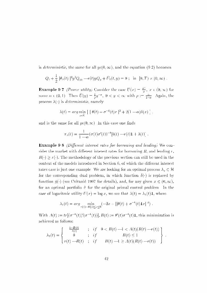
is deterministic, the same for all y�(0;1), and the equation (9.2) becomesQt + 12 jj��(t)jj2y2Qyy � r(t)yQy + ~U1(t; y) = 0 ; in [0; T )� (0;1) :Example 9.7 (Power utility) Consider the case U(x) = x�� ; x � (0;1) forsome � � (0; 1). Then ~U(y) = 1�y��; 0 < y < 1 with � := �1�� . Again, theprocess �(�) is deterministic, namely�(t) = argminx� ~K [ jj�(t) + ��1(t)xjj2 + 2(1� �)�(x) ] ;and is the same for all y�(0;1). In this case one �nds��(t) = 11� � (�(t)�0(t))�1[b(t)� r(t)1+ �(t)] :Example 9.8 (Di�erent interest rates for borrowing and lending) We con-sider the market with di�erent interest rates for borrowing R, and lending r,R(�) � r(�): The methodology of the previous section can still be used in thecontext of the models introduced in Section 6, of which the di�erent interestrates case is just one example. We are looking for an optimal process �y 2 Hfor the corresponding dual problem, in which function �(�) is replaced byfunction ~g(�) (see Cvitani�c 1997 for details), and, for any given x 2 (0;1),for an optimal portfolio � for the original primal control problem. In thecase of logaritmic utility U(x) = log x; we see that �(t) = �1(t)1, where�1(t) = arg minr(t)�R(t)�x�0(�2x+ jj�(t) + ��1(t)1xjj2) :With A(t) := tr[(��1(t))0(��1(t))]; B(t) := �0(t)��1(t)1, this minimization isachieved as follows:�1(t) = 8>><>>: 1�B(t)A(t) ; if 0 < B(t)� 1 < A(t)(R(t)� r(t))0 ; if B(t) � 1r(t)�R(t) ; if B(t)� 1 � A(t)(R(t)� r(t)) 9>>=>>; :42

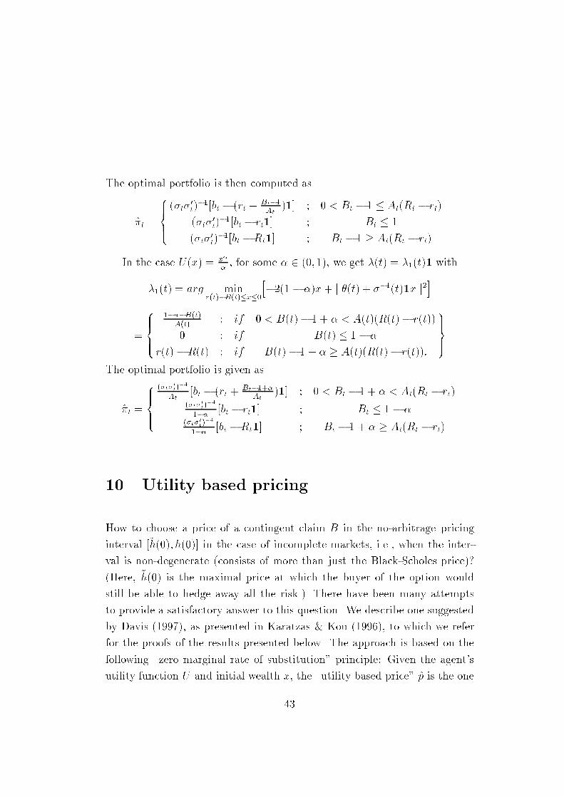
The optimal portfolio is then computed as�t = 8>><>>: (�t�0t)�1[bt � (rt + Bt�1At )1] ; 0 < Bt � 1 � At(Rt � rt)(�t�0t)�1[bt � rt1] ; Bt � 1(�t�0t)�1[bt �Rt1] ; Bt � 1 � At(Rt � rt)In the case U(x) = x�� ; for some � 2 (0; 1), we get �(t) = �1(t)1 with�1(t) = arg minr(t)�R(t)�x�0h�2(1 � �)x+ jj�(t) + ��1(t)1xjj2i= 8>><>>: 1���B(t)A(t) ; if 0 < B(t)� 1 + � < A(t)(R(t)� r(t))0 ; if B(t) � 1 � �r(t)�R(t) ; if B(t)� 1 + � � A(t)(R(t)� r(t)): 9>>=>>;The optimal portfolio is given as�t = 8>><>>: (�t�0t)�1At [bt � (rt + Bt�1+�At )1] ; 0 < Bt � 1 + � < At(Rt � rt)(�t�0t)�11�� [bt � rt1] ; Bt � 1 � �(�t�0t)�11�� [bt �Rt1] ; Bt � 1 + � � At(Rt � rt)10 Utility based pricingHow to choose a price of a contingent claim B in the no-arbitrage pricinginterval [~h(0); h(0)] in the case of incomplete markets, i.e., when the inter-val is non-degenerate (consists of more than just the Black-Scholes price)?(Here, ~h(0) is the maximal price at which the buyer of the option wouldstill be able to hedge away all the risk.) There have been many attemptsto provide a satisfactory answer to this question. We describe one suggestedby Davis (1997), as presented in Karatzas & Kou (1996), to which we referfor the proofs of the results presented below. The approach is based on thefollowing \zero marginal rate of substitution" principle: Given the agent'sutility function U and initial wealth x, the \utility based price" p is the one43

that makes the agent neutral with respect to diversion of a small amount offunds into the contingent claim at time zero, while maximizing the utilityfrom total wealth at the exercise time T . It can be shown thatp = E[H�x(T )B]; (10.1)where �x is the associated optimal dual process. In particular, this price canbe calculated in the context of examples of the previous section, and doesnot depend on U and x, in the case of cone constraints (� � 0) and constantcoe�cients (Example 9.6). It can also be shown that, in this case, it givesrise to the probability measure P�x which minimizes the relative entropy withrespect to the original measure P , among all measures P� , � 2 D.We describe now more precisely what we mean by \utility based price".For a given �x < � < x and price p of the claim, we introduce the valuefunction Q(�; p; x) := sup�2A0 0(x��)EU(Xx��(T ) + �pB): (10.2)In other words, the agent acquires �=p units of the claim B at price p attime zero, and maximizes his/her terminal wealth at time T . Davis (1997)suggests to use price p for which@Q@� (�; p; x)�����=0 = 0;so that this diversion of funds has a neutral e�ect on the expected utility.Since the derivative of Q need not exist, we have the followingDe�nition 10.1 For a given x > 0, we call p a weak solution of (10.2) if, forevery function ' : (�x; x) 7! R of class C1 which satis�es'(�) � Q(�; p; x);8� 2 (�x; x); '(0) = Q(0; p; x) = V (x);we have '0(0) = 0. If it is unique, then we call it the utility based price ofB.Theorem 10.1 Under the conditions of Theorem 8.2, the utility based priceof B is given as in (10.1). 44

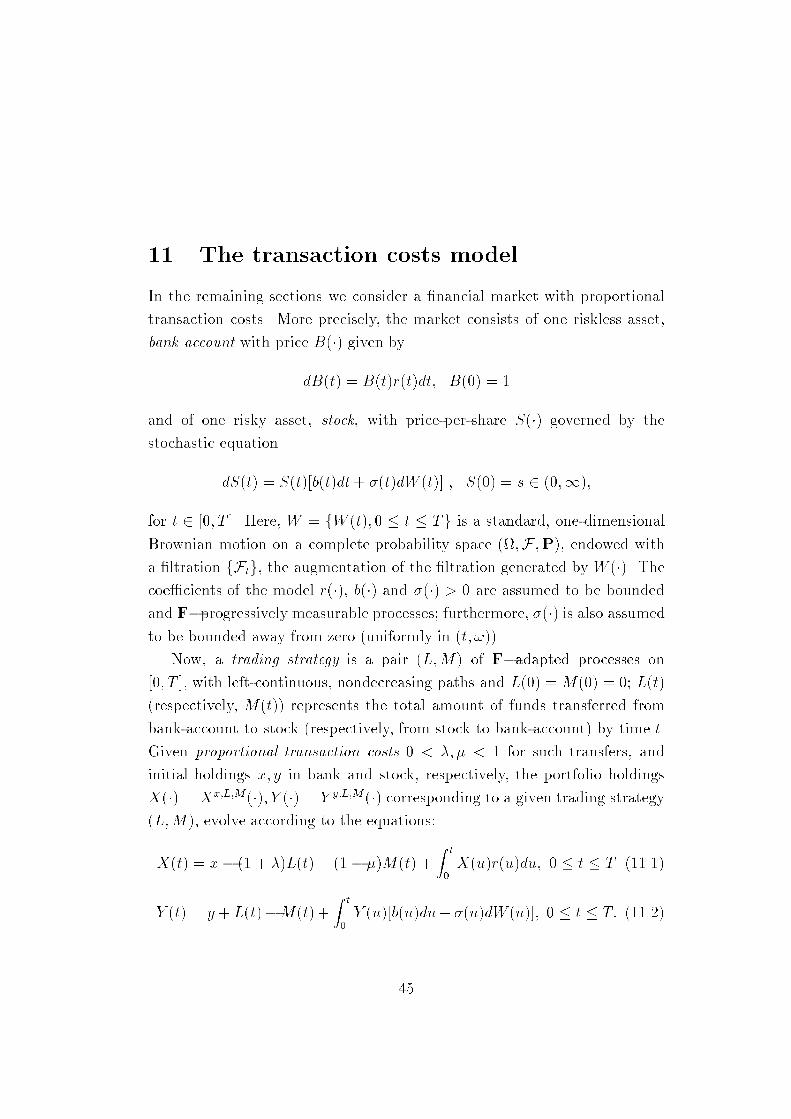
11 The transaction costs modelIn the remaining sections we consider a �nancial market with proportionaltransaction costs. More precisely, the market consists of one riskless asset,bank account with price B(�) given bydB(t) = B(t)r(t)dt; B(0) = 1and of one risky asset, stock, with price-per-share S(�) governed by thestochastic equationdS(t) = S(t)[b(t)dt+ �(t)dW (t)] ; S(0) = s 2 (0;1);for t 2 [0; T ]. Here, W = fW (t); 0 � t � Tg is a standard, one-dimensionalBrownian motion on a complete probability space (;F ;P), endowed witha �ltration fFtg, the augmentation of the �ltration generated by W (�). Thecoe�cients of the model r(�), b(�) and �(�) > 0 are assumed to be boundedand F�progressively measurable processes; furthermore, �(�) is also assumedto be bounded away from zero (uniformly in (t; !)).Now, a trading strategy is a pair (L;M) of F�adapted processes on[0; T ], with left-continuous, nondecreasing paths and L(0) =M(0) = 0; L(t)(respectively, M(t)) represents the total amount of funds transferred frombank-account to stock (respectively, from stock to bank-account) by time t.Given proportional transaction costs 0 < �; � < 1 for such transfers, andinitial holdings x; y in bank and stock, respectively, the portfolio holdingsX(�) = Xx;L;M(�); Y (�) = Y y;L;M (�) corresponding to a given trading strategy(L;M), evolve according to the equations:X(t) = x� (1 + �)L(t) + (1 � �)M(t) + Z t0 X(u)r(u)du; 0 � t � T (11.1)Y (t) = y+ L(t)�M(t) + Z t0 Y (u)[b(u)du+ �(u)dW (u)]; 0 � t � T: (11.2)45

De�nition 11.1 A contingent claim is a pair (C0; C1) of FT�measurablerandom variables. We say that a trading strategy (L;M) hedges the claim(C0; C1) starting with (x; y) as initial holdings, if X(�); Y (�) of (11.1), (11.2)satisfy X(T ) + (1� �)Y (T ) � C0 + (1� �)C1 (11.3)X(T ) + (1 + �)Y (T ) � C0 + (1 + �)C1: (11.4)Interpretation: HereC0 (respectively,C1) is understood as a target-positionin the bank-account (resp., the stock) at the terminal time t = T : for exampleC0 = �k1fS(T )>kg; C1 = S(T )1fS(T )>kgin the case of a European call-option; andC0 = k1fS(T )<kg; C1 = �S(T )1fS(T )<kgfor a European put-option (both with exercise price k � 0).\Hedging", in the sense of (11.3) and (11.4), simply means that one isable to cover these positions at t = T . Indeed, assume that we have bothY (T ) � C1 and (11.3), in the formX(T ) + (1 � �)[Y (T )� C1] � C0 ;then (11.4) holds too, and the agent can cover the position in the bank-account as well, by transferring the amount Y (T )� C1 � 0 to it. Similarlyfor the case Y (T ) < C1.The equations (11.1), (11.2) can be written in the equivalent formd X(t)B(t)! = 1B(t)! [(1� �)dM(t) � (1 + �)dL(t)] ; X(0) = x (11.5)d Y (t)S(t)! = 1S(t)! [dL(t)� dM(t)] ; Y (0) = y (11.6)in terms of \number-of-shares" (rather than amounts) held.46

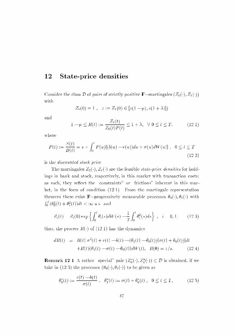
12 State-price densitiesConsider the class D of pairs of strictly positive F�martingales (Z0(�); Z1(�))with Z0(0) = 1 ; z := Z1(0) 2 [s(1� �); s(1 + �)])and 1 � � � R(t) := Z1(t)Z0(t)P (t) � 1 + �; 8 0 � t � T; (12.1)whereP (t) := S(t)B(t) = s+ Z t0 P (u)[(b(u)� r(u))du+ �(u)dW (u)] ; 0 � t � T(12.2)is the discounted stock price.The martingales Z0(�); Z1(�) are the feasible state-price densities for hold-ings in bank and stock, respectively, in this market with transaction costs;as such, they re ect the \constraints" or \frictions" inherent in this mar-ket, in the form of condition (12.1). From the martingale representationtheorem there exist F�progressively measurable processes �0(�); �1(�) withR T0 (�20(t) + �21(t))dt <1 a.s. andZi(t) = Zi(0) exp�Z t0 �i(s)dW (s)� 12 Z t0 �2i (s)ds� ; i = 0; 1; (12.3)thus, the process R(�) of (12.1) has the dynamicsdR(t) = R(t)[�2(t) + r(t)� b(t)� (�1(t)� �0(t))(�(t) + �0(t))]dt+R(t)(�1(t)� �(t)� �0(t))dW (t); R(0) = z=s: (12.4)Remark 12.1 A rather \special" pair (Z�0(�); Z�1 (�)) 2 D is obtained, if wetake in (12.3) the processes (�0(�); �1(�)) to be given as��0(t) := r(t)� b(t)�(t) ; ��1(t) := �(t) + ��0(t) ; 0 � t � T; (12.5)47

and let Z�0 (0) = 1; s(1 � �) � Z�1 (0) = z � s(1 + �): Because then, from(12.4), R�(�) := Z�1 (�)Z�0 (�)P (�) � zs ; in fact, the pair of (12.5) and z = s providethe only member (Z�0(�); Z�1 (�)) of D, if � = � = 0: Notice that the processes��0(�), ��1(�) of (12.5) are bounded.Let us observe also thatZ0(t)X(t)B(t) + Z1(t)Y (t)S(t) + Z t0 Z0(s)B(s) [(1 + �) �R(s)]dL(s)+ Z t0 Z0(s)B(s) [R(s)� (1 � �)]dM(s) (12.6)= x+ yzs + Z t0 Z0(s)B(s) [X(s)�0(s) +R(s)Y (s)�1(s)]dW (s); t 2 [0; T ]is a P�local martingale, for any (Z0(�); Z1(�)) 2 D and any trading strategy(L;M); this follows directly from (11.5), (11.6), (12.3) and the product rule.Equivalently, (12.6) can be re-written asX(t) +R(t)Y (t)B(t) + Z t0 (1 + �)�R(s)B(s) dL(s) + Z t0 R(s)� (1� �)B(s) dM(s)= x+ yzs + Z t0 R(s)Y (s)B(s) (�1(s)� �0(s))dW0(s); (12.7)where W0(t) := W (t)� Z t0 �0(s)ds; 0 � t � T (12.8)is a Brownian motion under the equivalent probability measureP0(A) := E[Z0(T )1A]; A 2 FT : (12.9)We shall denote by Z�0 (�);W �0 (�) and P�0 the processes and probabilitymeasure, respectively, corresponding to the process ��0(�) of (12.5), via theequations (12.3) (with Z�0 (0) = 1), (12.8) and (12.9). With this notation,(12.2) becomes dP (t) = P (t)�(t)dW �0 (t), P (0) = s.48

De�nition 12.1 Let D1 be the class of positive martingales (Z0(�); Z1(�)) 2D, for which the random variableZ0(T )Z�0 (T ); and thus also Z1(T )Z�0 (T )P (T ) ;is essentially bounded.De�nition 12.2 We say that a given trading strategy (L;M) is admissiblefor (x; y), and write (L;M) 2 A(x; y), ifX(�) +R(�)Y (�)B(�) is a P0� supermartingale, 8 (Z0(�); Z1(�)) 2 D1: (12.10)Consider, for example, a trading strategy (L;M) that satis�es the no-bankruptcyconditionsX(t) + (1 + �)Y (t) � 0 and X(t) + (1� �)Y (t) � 0; 8 0 � t � T:Then X(�) + R(�)Y (�) � 0 for every (Z0(�); Z1(�)) 2 D (recall (12.1), andnote Remark 12.2 below); this means that the P0�local martingale of (12.7)is nonnegative, hence a P0�supermartingale. But the second and the thirdterms Z �0 1 + ��R(s)B(s) dL(s); Z �0 R(s)� (1 � �)B(s) dM(s)in (12.7) are increasing processes, thus the �rst term X(�)+R(�)Y (�)B(�) is also aP0�supermartingale, for every pair (Z0(�); Z1(�)) inD. The condition (12.10)is actually weaker, in that it requires this property only for pairs in D1. Thisprovides a motivation for De�nition 12.2, namely, to allow for as wide a classof trading strategies as possible, and still exclude arbitrage opportunities. Thisis usually done by imposing a lower bound on the wealth process; however,that excludes simple strategies of the form \trade only once, by buying a�xed number of shares of the stock at a speci�ed time t", which may require(unbounded) borrowing. We will need to use such strategies in the sequel.49

Remark 12.2 Here is a trivial (but useful) observation: if x + (1 � �)y �a + (1 � �)b and x + (1 + �)y � a + (1 + �)b, then x + ry � a + rb;8 1� � � r � 1 + �:13 The minimal superreplication priceSuppose that we are given an initial holding y 2 R in the stock, and wantto hedge a given contingent claim (C0; C1) with strategies which are admis-sible (in the sense of De�nitions 11.1, 12.1. What is the smallest amount ofholdings in the bankh(C0; C1; y) := inffx 2 R= 9(L;M) 2 A(x; y) and (L;M) hedges (C0; C1)g(13.1)that allows to do this? We call h(C0; C1; y) the superreplication price of thecontingent claim (C0; C1) for initial holding y in the stock, and with theconvention that h(C0; C1; y) =1 if the set in (13.1) is empty.Suppose this is not the case, and let x 2 R belong to the set of (13.1);then for any (Z0(�); Z1(�)) 2 D1 we have from (12.10), the De�nition 11.1 ofhedging, and Remark 12.2:x+ ysEZ1(T ) = x+ ys z � E0 "X(T ) +R(T )Y (T )B(T ) #� E0 "C0 +R(T )C1B(T ) # = E "Z0(T )B(T ) (C0 +R(T )C1)# ;so that x � E hZ0(T )B(T ) (C0 +R(T )C1)� ysZ1(T )i. Thereforeh(C0; C1; y) � supD1 E "Z0(T )B(T ) (C0 +R(T )C1)� ysZ1(T )# ; (13.2)and this inequality is clearly also valid if h(C0; C1; y) =1.50

Lemma 13.1 If the contingent claim (C0; C1) is bounded from below, in thesenseC0+(1+�)C1 � �K and C0+(1��)C1 � �K; for some 0 � K <1 (13.3)thensupD1 E�Z0(T )B(T ) (C0 +R(T )C1) � ysZ1(T )�= supD E�Z0(T )B(T ) (C0 +R(T )C1)� ysZ1(T )�:Proof: Start with arbitrary (Z0(�); Z1(�)) 2 D and de�ne the sequence ofstopping times f�ng " T by�n := infft 2 [0; T ] = Z0(t)Z�0 (t) � ng ^ T; n 2 lN:Consider also, for i = 0; 1 and in the notation of (12.5):�(n)i (t) := ( �i(t); 0 � t < �n��i (t); �n � t � T )and Z(n)i (t) = zi expfZ t0 �(n)i (s)dW (s)� 12 Z t0 (�(n)i (s))2dsgwith z0 = 1; z1 = Z1(0) = EZ1(T ): Then, for every n 2 lN, both Z(n)0 (�) andZ(n)1 (�) are positive martingales, R(n)(�) = Z(n)1 (�)Z(n)0 (�)P (�) = R(� ^ �n) takes valuesin [1 � �; 1 + �] (by (12.1) and Remark 12.1), and Z(n)0 (�)=Z�0 (�) is boundedby n (in fact, constant on [�n; T ]): Therefore, (Z(n)0 (�); Z(n)1 (�)) 2 D1: Nowlet � denote an upper bound on K=B(T ), and observe, from Remark 12.2,(13.3) and Fatou's lemma:E "Z0(T )B(T ) (C0 +R(T )C1)� ysZ1(T )#+ ysZ1(0) + �= E "Z0(T )(C0 +R(T )C1B(T ) + �)#51

= E "limn Z(n)0 (T )(C0 +R(n)(T )C1B(T ) + �)#� limn E "Z(n)0 (T )(C0 +R(n)(T )C1B(T ) + �)#= limn E 24Z(n)0 (T )B(T ) (C0 +R(n)(T )C1)� ysZ(n)1 (T )35+ ysZ1(0) + �:This shows that the left-hand-side dominates the right-hand-side in the state-ment of the lemma; the reverse inequality is obvious. �Remark: Formally taking y = 0 in the above, we deduceE0 C0 +R(T )C1B(T ) ! � limn!1E(n)0 C0 +R(n)(T )C1B(T ) ! ; (13.4)where E0; E(n)0 denote expectations with respect to the probability measuresP0 of (12.9) and P(n)0 (�) = E[Z(n)0 (T )1�], respectively.Here is the main result of this section.Theorem 13.1 Under the conditions (13.3) andE�0(C20 + C21) <1 ; (13.5)we have h(C0; C1; y) = supD E "Z0(T )B(T ) (C0 +R(T )C1)� ysZ1(T )# :In (13.5), E�0 denotes expectation with respect to the probability measureP�0. The conditions (13.3), (13.5) are both easily veri�ed for a Europeancall or put. In fact, one can show that if a pair of admissible terminalholdings (X(T ); Y (T )) hedges a pair ( ~C0; ~C1) satisfying (13.5) (for example,( ~C0; ~C1) � (0; 0)), then necessarily the pair (X(T ); Y (T )) also satis�es (13.5){ and so does any other pair of random variables (C0; C1) which are boundedfrom below and are hedged by (X(T ); Y (T )). In particular, any strategywhich satis�es the \no-bankruptcy" condition of hedging (0; 0), necessarily52

results in a square-integrable �nal wealth. In this sense, the condition (13.5)is consistent with the standard \no-bankruptcy" condition, hence not veryrestrictive (this, however, is not necessarily the case if there are no transactioncosts).Proof: In view of Lemma 13.1 and the inequality (13.2), it su�ces to showh(C0; C1; y) � supD E "Z0(T ) C0B(T ) + Z1(T ) C1S(T ) � ys!# =: R: (13.6)For simplicity we take s = 1; r(�) � 0, thus B(�) � 1, for the remainder ofthe section; the reader will verify easily that this entails no loss of generality.We start by taking an arbitrary b < h(C0; C1; y) and considering the setsA0 := f(U; V ) 2 (L�2)2 : 9(L;M) 2 A(0; 0) that hedges (U; V ) starting withx = 0; y = 0g (13.7)A1 := f(C0 � b; C1 � yS(T ))g;where L�2 = L2(;FT ;P�0). It is not hard to prove (see below) thatA0 is a convex cone, and contains the origin (0; 0); in (L�2)2; (13.8)A0 \A1 = ;: (13.9)It is, however, considerably harder to establish thatA0 is closed in (L�2)2: (13.10)The proof can be found in the appendix of Cvitani�c & Karatzas (1996). From(13.8)-(13.10) and the Hahn-Banach theorem there exists a pair of randomvariables (��0; ��1) 2 (L�2)2; not equal to (0; 0), such thatE�0 [��0V0 + ��1V1] = E[�0V0 + �1V1] � 0; 8 (V0; V1) 2 A0 (13.11)E�0 [��0(C0�b)+��1(C1�yS(T ))] = E[�0(C0�b)+�1(C1�yS(T ))]� 0; (13.12)53

where �i := ��iZ�0 (T ); i = 0; 1. It is also not hard to check (see below) that(1 � �)E[�0jFt] � E[�1S(T )jFt]S(t) � (1 + �)E[�0jFt]; 8 0 � t � T (13.13)�1 � 0; �0 � 0 and E[�0] > 0; E[�1S(T )] > 0: (13.14)In view of (13.14), we may take E[�0] = 1, and then (13.12) givesb � E[�0C0 + �1(C1 � yS(T ))]: (13.15)Consider now arbitrary 0 < " < 1; (Z0(�); Z1(�)) 2 D, and de�ne~Z0(t) := "Z0(t) + (1� ")E[�0jFt]; ~Z1(t) := "Z1(t) + (1� ")E[�1S(T )jFt];for 0 � t � T: Clearly these are positive martingales, and ~Z0(0) = 1; on theother hand, multiplying in (13.13) by 1�", and in (1��)Z0(t) � Z1(t)=S(t) �(1 + �)Z0(t); 0 � t � T by ", and adding up, we obtain ( ~Z0(�); ~Z1(�)) 2 D:Thus, in the notation of (13.6),R � E " ~Z0(T )C0 + ~Z1(T ) C1S(T ) � y!#= (1 � ")E[�0C0 + �1(C1 � yS(T ))] + "E "Z0(T )C0 + Z1(T ) C1S(T ) � y!#� b(1� ") + "E "Z0(T )C0 + Z1(T ) C1S(T ) � y!#from (13.15); letting " # 0 and then b " h(C0; C1; y), we obtain (13.6), asrequired to complete the proof of Theorem 13.1.Proof of (13.9): Suppose that A0 \ A1 is not empty, i.e., that there exists(L;M) 2 A(0; 0) such that, with X(�) = X0;L;M (�) and Y (�) = Y 0;L;M(�), theprocess X(�) + R(�)Y (�) is a P0�supermartingale for every (Z0(�); Z1(�)) 2D1, and we have:X(T ) + (1� �)Y (T ) � (C0 � b) + (1 � �)(C1 � yS(T ));X(T ) + (1 + �)Y (T ) � (C0 � b) + (1 + �)(C1 � yS(T )):54

But then, with~X(�) := Xb;L;M(�) = b+X(�); ~Y (�) := Y y;L;M (�) = Y (�) + yS(�)we have, from above, that ~X(�)+R(�) ~Y (�) = X(�)+R(�)Y (�)+b+yZ1(�)=Z0(�)is a P0�supermartingale for every (Z0(�); Z1(�)) 2 D1, and that~X(T ) + (1� �) ~Y (T ) � C0 + (1� �)C1;~X(T ) + (1 + �) ~Y (T ) � C0 + (1 + �)C1:In other words, (L;M) belongs to A(b; y) and hedges (C0; C1) starting with(b; y) { a contradiction to the de�nition (13.1), and to the fact h(C0; C1; y) >b.Proof of (13.13), (13.14): Fix t 2 [0; T ) and let � be an arbitrary bounded,nonnegative, Ft�measurable random variable. Consider the strategy ofstarting with (x; y) = (0; 0) and buying � shares of stock at time s = t, oth-erwise doing nothing (\buy-and-hold strategy"); more explicitly,M �(�) � 0,L�(s) = �S(t)1(t;T ](s) and thusX�(s) := X0;L�;M�(�) = ��(1 + �)S(t)1(t;T ](s);Y �(s) := Y 0;L�;M�(s) = �S(s)1(t;T ](s);for 0 � s � T . Consequently, Z0(s)[X�(s) + R(s)Y �(s)] = �[Z1(s) � (1 +�)S(t)Z0(s)]1(t;T ](s) is a P�supermartingale for every (Z0(�); Z1(�)) 2 D,since, for instance with t < s � T :E[Z0(s)(X�s + RsY �s )jFt] = � (E[Z1(s)jFt]� (1 + �)StE[Z0(s)jFt])= �[Z1(t)� (1 + �)S(t)Z0(t)] = �S(t)Z0(t)[R(t)� (1 + �)]� 0 = Z0(t)[X�(t) +R(t)Y �(t)]:Therefore, (L�;M �) 2 A(0; 0), thus (X�(T ); Y �(T )) belongs to the set A0 of(13.7), and, from (13.11):0 � E[�0X�(T ) + �1Y �(T )] = E[�(�1S(T )� (1 + �)�0S(t))]55

= E[�(E[�1S(T )jFt]� (1 + �)S(t)E[�0jFt])]:From the arbitrariness of � � 0, we deduce the inequality of the right-handside in (13.13), and a dual argument gives the inequality of the left-handside, for given t 2 [0; T ). Now all three processes in (13.13) have continuouspaths; consequently, (13.13) is valid for all t 2 [0; T ].Next, we notice that (13.13) with t = T implies (1��)�0 � �1 � (1+�)�0,so that �0, hence also �1, is nonnegative. Similarly, (13.13) with t = 0 implies(1� �)E[�0] � E[�1S(T )] � (1 + �)E[�0], and therefore, since (�0; �1) is notequal to (0; 0), E[�0] > 0, hence also E[�1S(T )] > 0: This proves (13.14).�Remark 13.1 For the European call option with y = 0, we haveh(C0; C1; 0) = supD E "Z1(T )1fS(T )>kg � kZ0(T )B(T ) 1fS(T )>kg# ;and therefore, h(C0; C1; 0) � supD E[Z1(T )] = supD Z1(0) � (1 + �)s: Thenumber (1 + �)s corresponds to the cost of the \buy-and-hold strategy", ofacquiring one share of the stock at t = 0, and holding on to it until t = T:Davis & Clark (1994) conjectured that this hedging strategy is actually theleast expensive superreplication strategy:h(C0; C1; 0) = (1 + �)s:The conjecture was proved by Soner, Shreve & Cvitani�c (1995) by analyticmethods. Moreover, the following analogous result has been obtained inmore general continuous-time models and for more general contingent claimsby Levental & Skorohod (1997) (using probabilistic methods) and Cvitani�c,Pham & Touzi (1998) (using Theorem 13.1): \the cheapest buy-and-holdstrategy which dominates a given claim in a market with transaction costs isequal to its least expensive superreplication strategy". However, the result isnot always true, and, in particular, it does not hold for discrete-time models.56

14 Utility maximization under transaction costsConsider now a small investor who starts with initial capital (x; 0), x > 0,and derives utility U(X(T+)) from his terminal wealthX(T+) := X(T ) + f(Y (T )) � 0; where f(u) := ( (1 + �)u ; u � 0(1� �)u ; u > 0) :In other words, this agent liquidates at time T his position in the stock, incursthe appropriate transaction cost, and collects all the money in the bank-account. Denote by A+(x) the set of terminal holdings (X(T ); Y (T )) thathedge (0; 0), so that, in particular, X(T+) � 0. The agent's optimizationproblem is to �nd an admissible pair (L; M) 2 A+(x) thatmaximizes expectedutility from terminal wealth, i.e., attains the supremumV (x) := supA+(x)EU(X(T+)): (14.1)Here, U : (0;1) ! R is a strictly concave, strictly increasing, continuouslydi�erentiable utility function which satis�es U 0(0+) =1, U 0(1) = 0 andAssumption 14.1 The utility function U(x) has asymptotic elasticity strictlyless than 1, i.e. AE(U) := limx!1 xU 0(x)U(x) < 1: (14.2)It is shown in Kramkov & Schachermayer (1998) (henceforth [KS98]) thatthis condition is basically necessary and su�cient to ensure nice propertiesof value function V (x) and the existence of an optimal solution.We are again going to consider the dual problem. However, unlike thecase of portfolio constraints, we have to go beyond the set of state-pricedensities for the dual problem, and we introduce the setH := (Z 2 L0+ = E " ZB(T )(X(T ) + f(Y (T ))# � x; 8 (X(T ); Y (T )) 2 A+(x)) :(14.3)57

(Here, L0 is the set of all random variables on (;F ;P).) In particular, if(Z0(T ); Z1(T )) 2 D, then Z0(T ) 2 H. For a given z > 0, the auxiliary dualproblem associated with (14.1) is given by~V (z) := infZ2HE ~U(zZ=B(T )): (14.4)More precisely, similarly as in Cvitani�c & Karatzas (1996) (henceforth [CK96]),for every z > 0, Z 2 H and (X(T ); Y (T )) 2 A+(x) we haveEU(X(T+)) � E[ ~U(zZ=B(T )) +X(T+)Z=B(T )] � E ~U (zZ=B(T )) + zx:(14.5)Consequently, we haveV (x) � infz>0[ ~V (z) + zx] =: infz>0 (z): (14.6)Remark 14.1 The duality approach used in the market with portfolio con-straints suggests that we should look for pairs (z; Z) 2 (0;1) � H and(X(T+); 0) 2 A+(x) such the inequalities in (14.5) and (14.6) become equal-ities. The pair (X(T+); 0) is then optimal for (14.1). It is easily seen thatthis is the case (namely that those inequalities become equalities) if and onlyif (X(T+); 0) = I(zZ=B(T )); 0) 2 A+(x); E "ZI zZB(T )!# = x:We �rst state our results and then provide the proofs.Proposition 14.1 For every z > 0 there exists Zz 2 H that attains thein�mum in (14.4).Proposition 14.2 For every x 2 (0;1) there exists z 2 (0;1) that attainsthe in�mum of (z) in (14.6).Denote Z := Zz the optimal solution to (14.4) with z = z denoting theoptimal solution to infz>0 (z) of (14.6). The main result of this section isthe following 58

Theorem 14.1 The pair (C0; 0) := (I(zZ=B(T )); 0) belongs to the set A+(x)of (nonnegative) terminal holdings that can be hedged starting with initialwealth x > 0 in the bank account. Furthermore,E "U I zZB(T )!!# = V (x) = infz>0[ ~V (z) + zx] = ~V (z) + xz:In particular, the strategy that hedges (C0; 0) is optimal for the utility maxi-mization problem (14.1).Remark 14.2 Under Assumption 14.1, there exist z0 > 0, 0 < ; � < 1 and0 < c <1 such thatzI(z) < 1 � ~U (z) and ~U(�z) < c ~U (z); 8 0 < z < z0; (14.7)see [KS98] Lemma 6.3 and Corollary 6.1 for details.Proof of Proposition 14.1: We �rst observe that H is convex, closedunder a.s-convergence by Fatou's lemma, and bounded in L1(P); the latteris seen by setting (X(T ); Y (T )) = (xB(T ); 0) in (14.3), implying E[Z] � 1for Z 2 H. Fix z > 0 and let fZng be a minimizing sequence for (14.4).By Koml�os theorem (see Schwartz 1986), there exists a subsequence Z 0k suchthat ~Zk := 1k kXi=1 Z 0i ! Zz 2 Has k ! 1, almost surely. As in Lemma 3.4 of [KS98], Fatou's lemma isapplicable here, so that lim infk!1 E ~U(z ~Zk) � E ~U (zZz). In conjunctionwith convexity of ~U this easily implies that Zz is optimal for (14.4). �For a given progressively measurable process �(�) introduce the local mar-tingaleZ�(t) := expfZ t0 �(s)dW (s)� 12 Z t0 �2(s)dsg ; 0 � t � T: (14.8)59

In this section we will use the notation Z0 := Z��0 (T ) for the risk-neutraldensity for the market without transaction costs, where, as before, ��(t) :=(r(t)� b(t))=�(t). We have Z0 2 H.Lemma 14.1 Value function V (�) : (0;1) ! R is �nite, decreasing andstrictly convex.Proof: It is straightforward to check that ~V (�) is decreasing and strictlyconvex. Next, since r(�) is bounded, we have k�1 � B(T ) � k for somek > 0. In conjunction with Jensen's inequality, we obtainE ~U(zZ=B(T )) � ~U(zkE[Z]) � ~U (zk); (14.9)hence ~V (z) � ~U(zk) > �1: On the other hand, Assumption 14.1 ensuresthe existence of 0 < � < 1, z1 > 0 such that~U (�z1) < � ���1 ~U(z1) for all 0 < � < 1;see [KS98] Lemma 6.3 for the proof. We get, since Z0 2 H,~V (z) � E ~U (zZ0=B(T ))= E[ ~U(zZ0=B(T ))1fzZ0=B(T )>z1g] + E[ ~U(zZ0=B(T ))1fzZ0=B(T )�z1]g� j ~U(z1)j+ (z=z1) ���1 j ~U (z1)j � E h(Z0=B(T )) ���1 i <1:Proof of Proposition 14.2: We have ~V (0+) = ~U(0+), so limz#0 (z) =~U(0+) = U(1). Therefore, if U(1) =1, the in�mum (z) on [0;1) cannotbe attained at z = 0. Suppose now that U(1) <1 and that the in�mum isattained at z = 0, namely that infz>0 (z) = ~U (0+). Then we havex � ~U(0+) � ~U (zH)z � E[HI(zH)]for all H 2 H and z > 0. Leting z ! 0 we get x � 1, a contradiction.Therefore, either the in�mum of (z) is attained at a (unique) number z =60

zx 2 (0;1) or it is attained at z = 1. If the latter is the case, then thereexists a sequence zn !1 such that for zn large enough and a �xed z < zn,we have (by (14.9))x � ~V (z)� ~V (zn)zn � z � ~V (z)� ~U(znk)zn � z :Letting zn !1 we get x � 0 by de l'Hospital's Rule, a contradiction. �Lemma 14.2 ~V 0(z) = �E " ZB(T )I z ZB(T )!# = �x:Proof: Let h(z) := E[ ~U(zZ=B(T ))]. Then h(�) is convex, h(�) � ~V (�) andh(z) = ~V (z). These three facts easily imply ��h(z) � �� ~V (z) � �+ ~V (z) ��+h(z), where �� denotes the left and the right derivatives. Because of this,it is su�cient to prove the lemma with ~V replaced by h. It is easy to show,by monotone convergence theorem, that�+h(z) � �E " ZB(T )I z ZB(T )!# : (14.10)On the other hand,��h(z) � lim"!0+E "� ZB(T )I (z � ") ZB(T )!#We claim thatZB(T )I (z � ") ZB(T )! = ZB(T )I (z � ") ZB(T )!1fz ZB(T )�z0g+ ZB(T )I (z � ") ZB(T )! 1fz ZB(T )<z0gis uniformly integrable when � is small enough, where z0 is the number from(14.7). Indeed, the �rst term is dominated by ZB(T )I � z�"z z0�, which is uni-formly integrable when " is su�ciently small since E[ ZB(T )] � k � E[Z] � k.61

It follows from (14.7) that the second term is dominated by1z � " 1 � ~U (z � ") ZB(T )! ;which is in turn dominated by1z � " c1 � ~U zZB(T )!when " is small. The uniform integrability follows from E ��� ~U � zZB(T )���� <1.Therefore, we can use the Mean Convergence Criterion to get the inequal-ity ��h(z) � �E " ZB(T )I z ZB(T )!# :Together with (14.10) we establish h0(z) = �E[ ZB(T )I(z ZB(T ))] = �x. Thelatter equality follows from the fact that z attains infz>0[ ~V (z) + xz]. �Lemma 14.3 We havesupZ2HE " ZB(T )I z ZB(T )!# = E " ZB(T )I z ZB(T )!# = x:Proof: For a given Z 2 H, " 2 (0; 1), let Z" := (1 � ")Z + "Z 2 H. Byoptimality of Z we get0 � 1"E " ~U zZB(T )!� ~U zZ"B(T )!# � �1"E " z(Z � Z")B(T ) I zZ"B(T )!#= E " z(Z � Z)B(T ) I zZ"B(T )!# : (14.11)However, it follows that, as in the proof of Lemma 14.2, Z � ZB(T ) I zZ"B(T )!!� � ZB(T )I z(1� ")ZB(T ) !62

is uniformly integrable. We can now use Fatou's lemma in (14.11), to getE "Z � ZB(T ) I zZB(T )!# � 0;which completes the proof. �Proof of Theorem 14.1: For �xed x > 0 de�neC := f� 2 L0+ = xB(T )� � X(T )+f(Y (T )); for some (X(T ); Y (T )) 2 A+(x)g:Denote by C0 := fZ 2 L0+ = E[Z�] � 1; 8 � 2 Cgthe polar of set C. It is clear then that H = C0. We also want to showC = H0 = C00. By the bipolar theorem of Brannath & Schachermayer(1998), it is su�cient to show that C is convex, solid and closed under a.s.-convergence (a subset C of L0+ is solid if f 2 C and 0 � g � f imply g 2 C).It is obvious that C is convex and solid. On the other hand, from Theorem13.1 we know that � 2 C if and only ifE�0 [(�B(T ))2] <1 and supZ2HE[Z�] � 1:This implies (by Fatou's lemma) that C is closed under a.s-convergence, be-cause the set f�B(T )g�2C is bounded in L2(P�0). Indeed, the latter followsfrom [CK96] (as remarked in Appendix B of that paper, this can be shownby setting Un = Vn = 0 in the arguments of its Appendix A; see (A.8)-(A.11) on p156). We conclude that C = H0. Now, Lemma 14.3 impliesI(zZ=B(T ))xB(T ) 2 H0 = C, hence (I(zZ=B(T )); 0) 2 A+(x): This, in conjunctionwith Lemma 14.3 and Remark 14.1, implies the remaining statements of thetheorem.�Notice that, if r(�) is deterministic, then Jensen's inequality givesE " ~U z ZB(T )!# � ~U zB(T )E[Z]!63

� ~U zB(T )! ; (14.12)for all Z 2 H. We will use this observation to �nd examples, in which theoptimal strategy (L; M) never trades.Example 14.9 Let us assume that r(�) is deterministic. In this case we seefrom (14.12) that ~V (z) � ~U(z=B(T ));and the in�mum is attained by taking Z � 1, if 1 2 H. A su�cient conditionfor this is (1; Z1(�)) 2 D for some positive martingale Z1(�) such that 1�� �R(�) = Z1(�)=P (�) � 1 + �. In particular, one can set Z1(0) = (1 + �)s andZ1(�) = Z�1 (�), where �1(�) � �(�), in which case (1; Z1(�)) 2 D if and only if0 � Z t0 (b(s)� r(s))ds � log 1 + �1� � ;8 0 � t � T: (14.13)Furthermore, X(T+) = I(z=B(T )) = xB(T ):This means that the no-trading-strategy L � 0, M � 0 is optimal. Condition(14.13) is satis�ed, for instance, ifr(�) � b(�) � r(�) + � ; for some 0 � � � 1T log 1 + �1 � �: (14.14)If b(�) = r(�) the result is not surprising { even without transaction costs, itis then optimal not to trade. However, if there are no transaction costs, inthe case b(�) > r(�) the optimal portfolio always invests a positive amount inthe stock; the same is true even in the presence of transaction costs, if oneis maximizing expected discounted utility from consumption over an in�nitetime-horizon, and if the market coe�cients are constant { see Shreve & Soner(1994), Theorem 11.6. The situation here, on the �nite time-horizon [0; T ],is quite di�erent: if the excess rate of return b(�)� r(�) is positive but smallrelative to the transaction costs, and/or if the time-horizon is small, in thesense of (14.14), then it is optimal not to trade.64

ReferencesAVELLANEDA, M. & PAR�AS, A. (1994) Dynamic hedging portfolios forderivative securities in the presence of large transaction costs. AppliedMathematical Finance 1, 165-194.BARLES, G. & SONER, H.M. (1998) Option pricing with transaction costsand a nonlinear Black-Scholes equation. Finance & Stochastics 4, 369-398.BENSAID, B., LESNE, J., PAG�ES, H. & SCHEINKMAN, J. (1992) Deriva-tive asset pricing with transaction costs. Mathematical Finance 2 (2), 63-86.BERGMAN, Y.Z. (1991) Option pricing with di�erential interest rates. Rev.Financial Studies 8, 475-500.BISMUT, J.M. (1973) Conjugate convex functions in optimal stochastic con-trol. J. Math. Analysis & Applic. 44, 384-404.BISMUT, J.M. (1975) Growth and optimal intertemporal allocations of risks.J. Economic Theory 10, 239-287.BLACK, F. & SCHOLES, M. (1973) The pricing of options and corporateliabilities. J. Polit. Economy 81, 637-659.BOYLE, P. P. & VORST, T. (1992) Option replication in discrete time withtransaction costs. J. Finance 47, 272-293.BRANNATH,W. & SCHACHERMAYER, W. (1998) A bipolar theorem forsubsets of L0+(;F ; P ). To appear in S�eminaire de Probabilit�es.BROADIE, M., CVITANI�C, J. & SONER, H. M. (1998) On the cost ofsuper-replication under portfolio constraints. Rev. of Financial Studies11, 59-79.CONSTANTINIDES, G.M. (1979) Multiperiod consumption and investmentbehavior with convex transaction costs. Management Sci. 25, 1127-1137.CONSTANTINIDES, G.M. & ZARIPHOPOULOU, T. (1999) Bounds onprices of contingent claims in an intertemporal economy with propor-tional transaction costs and general preferences. Finance & Stochastics65

3, 345-370.COX, J. & HUANG,C. F. (1989) Optimal consumption and portfolio policieswhen asset prices follow a di�usion process. J. Econ. Theory 49, 33-83.COX, J. & HUANG, C. F. (1991) A variational problem arising in �nancialeconomics. J. Math. Economics 20, 465-487.CUOCO, D & CVITANI�C, J. (1998) Optimal consumption choices for alarge investor. J. Econ. Dynamics and Control 22, 401-436.CVITANI�C, J. (1997) Nonlinear �nancial markets: hedging and portfoliooptimization. In Mathematics of Derivative Securities, M.H.A. Demp-ster and S. Pliska Eds., Proc. of the Isaac Newton Institute, CambridgeUniversity Press.CVITANI�C, J. & KARATZAS, I. (1992) Convex duality in constrained port-folio optimization. Ann. Appl. Probab. 2, 767-818.CVITANI�C, J. & KARATZAS, I. (1993) Hedging contingent claims withconstrained portfolios. Ann. Appl. Probab. 3, 652-681.CVITANI�C, J. & KARATZAS, I. (1996) Hedging and portfolio optimizationunder transaction costs: a martingale approach. Mathematical Finance6, 133-165.J. CVITANI�C, H. PHAM & N. TOUZI (1998) A closed form solution tothe problem of super-replication under transaction costs. Finance &Stochastics 3, 35-54.CVITANI�C, J. & WANG, H. (1999) On optimal terminal wealth under trans-action costs. J. of Math. Economics, to appear.DAVIS, M.H.A. (1997) Option pricing in incomplete markets. In Mathemat-ics of Derivative Securities, M.A.H. Dempster and S. Pliska Eds., Proc.of the Isaac Newton Institute, Cambridge University Press.DAVIS, M. H .A. & CLARK, J. M. C. (1994) A note on super-replicatingstrategies. Phil. Trans. Royal Soc. London A 347, 485-494.DAVIS, M. H. A. & NORMAN, A. (1990) Portfolio selection with transactioncosts. Math. Operations Research 15, 676-713.DAVIS, M. H. A. & PANAS, V. G. (1994) The writing price of a European66

contingent claim under proportional transaction costs. Comp. Appl.Math. 13, 115-157.DAVIS,M. H. A., PANAS, V. G. & ZARIPHOPOULOU,T. (1993) Europeanoption pricing with transaction costs. SIAM J. Control & Optimization31, 470-493.DAVIS, M. H. A. & ZARIPHOPOULOU, T. (1995) American options andtransaction fees. InMathematical Finance, M. H. A. Davis et al. ed., TheIMA Volumes in Mathematics and its Applications 65, 47-62. Springer-Verlag.EDIRISINGHE, C., NAIK, V. & UPPAL, R. (1993) Optimal replication ofoptions with transaction costs and trading restrictions. J. Financial &Quantitative Analysis 28, 117-138.EKELAND, I. & TEMAM, R. (1976) Convex Analysis and Variational Prob-lems. North-Holland, Amsterdam and Elsevier, New York.EL KAROUI, N., PENG, S. & QUENEZ, M.C. (1997) Backward StochasticDi�erential Equations in �nance. Math. Finance 7, 1-71.EL KAROUI, N. & QUENEZ, M.C. (1995) Dynamic programming and pric-ing of contingent claims in an incomplete market. SIAM J. Control &Optimization, 33, 29-66.FLEMING, W.H. & SONER, H.M. (1993) Controlled Markov Processes andViscosity Solutions. Springer-Verlag, New York.FLEMING, W. & ZARIPHOPOULOU, T. (1991) An optimal investment/consumption model with borrowing. Math. Oper. Res. 16 802-822.FLESAKER, B. & HUGHSTON, L. P. (1994) Contingent claim replicationin continuous time with transaction costs. Proc. Derivative SecuritiesConference, Cornell University.FOLDES, L. (1978a) Martingale conditions for optimal saving - discrete time.J. Math. Economics 5, 83-96.FOLDES, L. (1978b) Optimal saving and risk in continuous time. Rev. Eco-nomic Studies 45, 39-65.F�OLLMER, H. & KRAMKOV, D. (1997) Optional decomposition under67

constraints. Prob Theory and Related Fields 109, 1-25.GILSTER, J. E. & LEE, W. (1984) The e�ect of transaction costs and di�erent borrowing and lending rates on the option pricing model. J. Finance43, 1215-1221.GRANNAN, E.R. & SWINDLE, G.H. (1996) Minimizing transaction costsof option hedging strategies. Mathematical Finance 6, 239-253.HARRISON, J. M. & KREPS, D. M. (1979) Martingales and arbitrage inmultiperiod security markets. J. Econom. Theory 20, 381{408.HARRISON, J. M. & PLISKA, S. R. (1981) Martingales and stochastic inte-grals in the theory of continuous trading. Stochastic Processes and Appl.11, 215{260.HARRISON, J. M. & PLISKA, S. R. (1983) A stochastic calculus modelof continuous time trading: complete markets. Stochastic Processes andAppl. 15, 313{316.HE, H. & PEARSON, N. (1991) Consumption and portfolio policies withincomplete markets and short-sale constraints: The in�nite-dimensionalcase. J. Econ. Theory 54, 259-304.HODGES, S.D. & NEUBERGER, A. (1989) Optimal replication of contin-gent claims under transaction costs. Review of Future Markets 8, 222-239.HOGGARD, T., WHALLEY, A.E., & WILMOTT, P. (1994) Hedging optionportfolios in the presence of transaction costs. Adv. in Futures andOptions Research, 7, 21-35.JOUINI, E. & KALLAL, H. (1995a) Arbitrage in securities markets withshort-sale constraints. Math. Finance 5, 197-232.JOUINI, E. & KALLAL, H. (1995b) Martingales and arbitrage in securitiesmarkets with transaction costs. J. Econ. Theory 66, 178-197.KABANOV, Yu.M. (1999) Hedging and liquidation under transaction costsin currency markets. Finance & Stochastics 3, 237-248.KARATZAS, I. & KOU, S-G. (1996) On the pricing of contingent claimsunder constraints. The Annals of Applied Probability., 6, 321-369.68

KARATZAS, I., LEHOCZKY, J. P. & SHREVE, S. E. (1987) Optimal port-folio and consumption decisions for a \small investor" on a �nite horizon.SIAM J. Control Optimization 25, 1557-1586.KARATZAS, I., LEHOCZKY, J. P., SHREVE, S. E. & XU, G. L. (1991)Martingale and duality methods for utility maximization in an incom-plete market. SIAM J. Control Optimization 29, 702-730.KARATZAS, I. & SHREVE, S.E. (1991) Brownian Motion and StochasticCalculus (2nd edition), Springer-Verlag, New York.KARATZAS, I. & SHREVE, S.E. (1998) Methods of Mathematical Finance.Springer-Verlag, New York.KOML�OS, J. (1967) A generalization of a problem of Steinhaus. Acta Math.Acad. Sci. Hungar. 18, 217-229.KORN, R. (1997) Optimal Portfolios : Stochastic Models for Optimal In-vestment and Risk Management in Continuous Time. World Scienti�c,Singapore.KRAMKOV, D. & SCHACHERMAYER, W. (1998) The asymptotic elas-ticity of utility functions and optimal investment in incomplete markets.The Annals of Applied Probability 9.KUSUOKA, S. (1995) Limit theorem on option replication with transactioncosts. Ann. Appl. Probab. 5, 198-221.LADY�ZENSKAJA,O.A., SOLONNIKOV,V.A. & URAL'TSEVA,N.N. (1968)Linear and Quasilinear Equations of Parabolic Type. Translations ofMathematical Monographs, Vol. 23, American Math. Society, Provi-dence, R.I.LELAND, H.E. (1985) Option pricing and replication with transaction costs.J. Finance 40, 1283-1301.LEVENTAL, S. & SKOROHOD, A. V. (1997) On the possibility of hedgingoptions in the presence of transactions costs. Ann. Appl. Probab. 7,410-443.MAGILL, M.J.P. & CONSTANTINIDES, G.M. (1976) Portfolio selectionwith transaction costs. J. Economic Theory 13, 264-271.69

CONSTANTINIDES, G.M. (1979) Multiperiod consumption and investmentbehavior with convex transaction costs. Management Sci. 25, 1127-1137.MERTON, R.C. (1969) Lifetime portfolio selection under uncertainty:the continuous-time case. Rev. Econom. Statist., 51, 247-257.MERTON, R.C. (1971) Optimumconsumption and portfolio rules in a continuous-time model. J. Econom. Theory 3, 373-413. Erratum: ibid 6 (1973),213-214.MERTON, R. C. (1989) On the application of the continuous time theoryof �nance to �nancial intermediation and insurance, The Geneva Paperson Risk and Insurance, 225{261.MERTON, R.C. (1990) Continuous-Time Finance. Basil Blackwell, Oxfordand Cambridge.MORTON, A. J. & PLISKA, S. R. (1995) Optimal portfolio managementwith �xed transaction costs, Math. Finance 5, 337-356.NEVEU, J. (1975) Discrete-Parameter Martingales. North-Holland, Ams-terdam.PLISKA, S. (1986) A stochastic calculus model of continuous trading: opti-mal portfolios. Math. Oper. Res. 11, 371-382.PLISKA, S. (1997) Introduction to Mathematical Finance. Discrete TimeModels. Blackwell, Oxford.ROCKAFELLAR, R.T. (1970) Convex Analysis. Princeton University Press,Princeton.SCHWARTZ, M. (1986) New proofs of a theorem of Koml�os. Acta Math.Hung. 47, 181-185.SHREVE, S. E. & SONER, H. M. (1994) Optimal investment and consump-tion with transaction costs, Ann. Appl. Probab. 4, 609-692.SONER, H. M., SHREVE, S. E. & CVITANI�C, J. (1995) There is no non-trivial hedging portfolio for option pricing with transaction costs, Ann.Appl. Probab. 5, 327-355.TAKSAR, M., KLASS, M.J. & ASSAF, D. (1988) A di�usion model foroptimal portfolio selection in the presence of brokerage fees, Math. Op-70

erations Research 13, 277-294.XU, G.L. (1990) A Duality Method for Optimal Consumption and Investmentunder Short-Selling Prohibition. Doctoral Dissertation, Carnegie-MellonUniversity.XU, G. & SHREVE, S. E. (1992) A duality method for optimal consumptionand investment under short-selling prohibition. I. General market coef-�cients. II. Constant market coe�cients. Ann. Appl. Probab. 2, 87-112,314-328.ZARIPHOPOULOU, T. (1992) Investment/consumption model with trans-action costs and Markov-chain parameters. SIAM J. Control Optimiza-tion 30, 613-636.

71