Electricity Demand Forecasting using Multi-Task Learning · PDF fileElectricity Demand...

Electricity Demand Forecasting using Multi-Task Learning

Jean-Baptiste Fiot, Francesco Dinuzzo

Dublin Machine Learning Meetup - July 2017

1 / 32N

Outline

1 Introduction

2 Problem Formulation

3 Kernels

4 Experiments

5 Conclusion

2 / 32N

Outline

1 Introduction


3 Kernels

4 Experiments

5 Conclusion

3 / 32N

Electricity Demand Forecasting

Electricity is a special commodity

It cannot be stored efficiently (in large quantities)

It looses value when being moved (line losses)

Demand forecasting is critical

Operations, bidding, demand response, maintenance, planning, etc.

The game is changing

Distributed renewable generation

Higher volatility on markets

Increased number of participants

4 / 32N

Demand Forecasting Methods

(Non-)linear variants of least-squares, ARMAX, fuzzy logic, etc.

Black-box models based on neural networks [Hippert et al., 2001]

Generalized Additive Models (GAM)

Great performance [Fan and Hyndman, 2012, Ba et al., 2012]

Efficient and scalable training algorithms

Interpretability of the model

Hippert, HS, et al.Neural networks for short-term load forecasting: A review and evaluation.Power Systems, IEEE Transactions on, 16(1):44–55, 2001.

Fan, S and Hyndman, R.Short-term load forecasting based on a semi-parametric additive model.Power Systems, IEEE Transactions on, 27(1):134–141, 2012.

Ba, A, et al.Adaptive learning of smoothing functions: application to electricity load forecasting.In Advances in Neural Information Processing Systems 25 (NIPS 2012), pages 2519–2527. 2012.

5 / 32N

Demand Forecasting using Kernel Methods

In 2001, kernel-based support vector regression won EUNITE(European Network on Intelligent Technologies for Smart AdaptiveSystems) demand forecasting competition [Chen et al., 2004]

Later, kernel-based regularizations and support vectortechniques were successfully used[Espinoza et al., 2007, Hong, 2009, Elattar et al., 2010]

Chen, B, et al.Load forecasting using support vector machines: A study on EUNITE competition 2001.Power Systems, IEEE Transactions on, 19(4):1821–1830, 2004.

Espinoza, M, et al.Electric load forecasting.Control Systems, IEEE, 27(5):43–57, 2007.

Hong, WC.Electric load forecasting by support vector model.Applied Mathematical Modelling, 33(5):2444–2454, 2009.

Elattar, E, et al.Electric load forecasting based on locally weighted support vector regression.Systems, Man, and Cybernetics, Part C: Applications and Reviews, IEEE Transactions on,40(4):438–447, 2010.

6 / 32N

Outline

1 Introduction


3 Kernels

4 Experiments

5 Conclusion

7 / 32N

Electric Demand Forecasting

y = f (t, d , c , yl , ul , j , sj) ,

Time/Calendar features

t ∈ [0, 24) is the time of day expressed in hours,

d ∈ {1, 2, . . . , 365, 366} is the day of the year,

c is the type of day, e.g. Monday to Sunday,

Dynamic features

yl is a real vector containing lagged values of the electric demand,

ul is a real vector containing measurements of lagged values ofexogenous variables other than the demand (such as temperature),

Meter features

j is the meter ID in the electricity network,

sj is a vector of features describing the demande measured at j .

8 / 32N

Solving Multiple Demand Forecasting Problems

Consider m smart meters, indexed by j

Goal: learn {fj : X → R}1≤j≤m from datasets (xij , yij) ∈ X × R.

9 / 32N

Optimisation Problem

Letting f : X → Rm the function with components fj , we minimize

R(f ,L) =m∑j=1

`j∑i=1

(yij − fj(xij)))2 + λ‖f ‖2HL, (1)

where λ > 0 is a regularization parameter, and HL is a Reproducing KernelHilbert Space (RKHS) of vector-valued functions with (matrix-valued) kernel

H(xi , xj ) = K(xi , xj ) · L , (2)

K : X × X → R is the input kernel, and L ∈ Rm×m is the output kernel.

Representer theorem: there exist functions fj minimizingR(f ,L) in the form:

fj(x) =m∑

k=1

Ljk

`k∑i=1

cikK (xik , x). (3)

10 / 32N

Fixing L = I: Independent Kernel Ridge Regression

11 / 32N

Learning L = I: Output Kernel Learning

Remark: B = (bij ) is a Cholesky factor of L

12 / 32N

Output Kernel Learning

Joint optimization problem

minL∈Sm,p

+

minf∈HL

R(f ,L) + λtr(L) ,

where Sm,p+ is the cone of p.s.d. matrices with rank ≤ p.

Re-indexing the observations {xi}i=1,...,`, the solution becomes

fj(x) =

p∑k=1

bjkgk(x), gk(x) =∑i=1

aikK (xi , x) ,

where

{bjkcoefficients form a low-rank factor of L ,

gk functions can be seen as modes or typical profiles .

It is sufficient to store (`+ m)p parameters, which can be muchsmaller than

∑mj=1 `j .

13 / 32N

Outline

1 Introduction


3 Kernels

4 Experiments

5 Conclusion

14 / 32N

Multiple Seasonalities in Electricity Demand

Figure: French National Demand (Reseau de Transport d’Electricite data)15 / 32

N

Capturing Demand Seasonalities with Kernels

Time-of-day kernel

K t(t1, t2) = exp (−hT (|t1 − t2|)/σt) , (4)

Day-of-year kernel

K d(d1, d2) = exp (−hD(|d1 − d2|)/σd) , (5)

where hP (x) = min{x, P − x} is a change of variable that yields P-periodic kernels over the square

[0, P]2. In our experiment, σt and σd were respectively set to 4 hours and 120 days.

Day-type kernel

K c(c1, c2) =

{1 if c1 = c2

0 if c1 6= c2.. (6)

16 / 32N

Kernels for Electric Demand Forecasting

To define K ((t1, d1, c1), (t2, d2, c2)), we combine the basis kernels

Additive Models

K t(t1, t2) + K d(d1, d2) , (7)

K t(t1, t2) + K d(d1, d2) + K c(c1, c2) , (8)

Semi-Additive Models

K d(d1, d2) + K t(t1, t2) · K c(c1, c2) , (9)(K t(t1, t2) + K d(d1, d2)

)· K c(c1, c2) , (10)

Multiplicative Models

K t(t1, t2) · K d(d1, d2) , (11)

K t(t1, t2) · K d(d1, d2) · K c(c1, c2) . (12)

17 / 32N

Outline

1 Introduction


3 Kernels

4 Experiments

5 Conclusion

18 / 32N

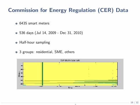
Commission for Energy Regulation (CER) Data

6435 smart meters

536 days (Jul 14, 2009 - Dec 31, 2010)

Half-hour sampling

3 groups: residential, SME, others

19 / 32N

Pre-processing

Removed two corrupted meters

Corrected DST measurements

Downsampled to 3-hour resolution

Final dataset:

m = 6433 smart meters

` = 4288 time slots

Customer group Meters Sparsity

Residential 4225 0.028%Industrial (SME) 485 0.035%Others 1723 17%

20 / 32N

Learning the Models

Data split

1 year (2920 obs.) used for training (80%) and validation (20%)

∼ 0.5 year (1368 obs.) used for testing

Independent Kernel Ridge Regression using the 6 kernels

Output Kernel Learning using MM2

1 model for {residential} ∪ {others}, p = 200 to fit in memory

1 model for {SME}, full rank (p = 485)

21 / 32N

Qualitative Analysis

2010−11−28 2010−12−05 2010−12−12 2010−12−19 2010−12−262000

3000

4000

5000

6000

7000

8000

2010−11−28 2010−12−05 2010−12−12 2010−12−19 2010−12−26

4

6

8

10

12

2010−11−28 2010−12−05 2010−12−12 2010−12−19 2010−12−26

0.5

1

1.5

2

2.5

3

Figure: Measured load (blue), indep. KRR (red) and multi-task OKL(black) forecasts for the aggregated demand (top), a single SME meter(middle), and a single residential meter (bottom).

22 / 32N

Performance Metrics (1/2)

Given a group of meters G and observation i , we define

Absolute percentage error (APE)

APE(i ,G) = 100

∣∣∣∣∣∑

j∈Gi yij −∑

j∈Gi fj(ti , di , ci )∑j∈Gi yij

∣∣∣∣∣ , (13)

where Gi is the subset of meters with available observations at i .

Normalized absolute error (NAE)

NAE(i ,G) =

∑j∈Gi |yij − fj(ti , di , ci )|∑

j∈Gi yij, (14)

23 / 32N

Performance Metrics (2/2)

Mean absolute percentage error (MAPE)

MAPE(G) =1

# T

∑i∈T

APE(i ,G) , (15)

Mean normalized absolute error (MNAE)

MNAE(G) =1

# T

∑i∈T

NAE(i ,G) . (16)

24 / 32N

Prediction Accuracy (1/2)

Overall Residential SME Others0.25

0.30

0.35

0.40

0.45

0.50

0.55

MN

AE a

nd s

tand

ard

erro

r

Additive Model 1Additive Model 2Semi-Additive Model 1Semi-Additive Model 2Multiplicative Model 1Multiplicative Model 2Multi-Task OKL

Overall Residential SME Others0

2

4

6

8

10

12

14

16

18

MAP

E an

d st

anda

rd e

rror

Additive Model Additive Model 2Semi-Additive Model 1Semi-Additive Model 2Multiplicative Model 1Multiplicative Model 2Multi-Task OKL

1 Multiplicative kernels outperform (semi-)additive models.

Multiplicative kernels lead to a stricter selection of training obs.

EUNITE winners discarded ≥ 90% of the dataset.

2 Multi-task OKL outperforms independent kernel ridge regression

The multi-task approach efficiently exploits the similarities

44% improvement of σAPE for SME against 2nd best method

25 / 32N

Prediction Accuracy (2/2)

AM 1 AM 2 SAM 1 SAM 2 MM 1 MM 2 OKL

OKL

MM

2M

M 1

SAM

2SA

M 1

AM 2

AM 1

10-4

10-3

10-2

10-1

100

(a) NAE

AM 1 AM 2 SAM 1 SAM 2 MM 1 MM 2 OKLO

KLM

M 2

MM

1SA

M 2

SAM

1AM

2AM

1

10-4

10-3

10-2

10-1

100

(b) APE

Figure: p-values of Welch t-test between the overall accuracies of allmethods on the CER dataset

26 / 32N

Basis Load Profiles gk

Jul 14, 09 Jul 18, 09 Jul 22, 09 Jul 26, 09 Jul 30, 09 Aug 03, 09 Aug 07, 09

Figure: CER Data: Typical load profiles displayed over the horizon of onemonth, obtained from a low-rank OKL model with p = 10.

27 / 32N

Number of Parameters

In this experiment, the OKL model is 4.24 times more compact.

Single-task: # params = # obs. =∑m

j=1 `j ≈ 1.3 · 107

Multi-task OKL: # params = (`+ m)p ≈ 3 · 106

28 / 32N

Relationships between Smart Meters

-1

-0.8

-0.6

-0.4

-0.2

0

0.2

0.4

0.6

0.8

1

Figure: CER data: entries of the normalized output kernel Ln ∈ Rm×m fora subset containing 50 residential and 50 SME (small or mediumenterprise) customers. (Ln)ij =

Lij√Lii×Ljj

, i , j = 1, . . . ,m.

29 / 32N

Outline

1 Introduction


3 Kernels

4 Experiments

5 Conclusion

30 / 32N

Contributions

1 We formulated the problem of forecasting the demand measured onmultiple lines of the network as a multi-task problem.

2 We designed kernels able to capture the seasonal effects presentin electricity demand data.

3 We exposed the performance limits of the very popular additivemodels, showing that they are often outperformed by multiplicativekernel models.

4 We showed how MTL can be used to gain insights andinterpretability on real demand data

31 / 32N

Thank You

Any question?

Contact details

Jean-Baptiste Fiot

[email protected]

32 / 32N

mailto:[email protected]

Electricity Demand Forecasting using Multi-Task Learning · PDF fileElectricity Demand...

Documents

Transcript of Electricity Demand Forecasting using Multi-Task Learning · PDF fileElectricity Demand...