Purdue UniversityPurdue e-Pubs

CTRC Research Publications Cooling Technologies Research Center

1-1-2012

Electrical impedance-based void fractionmeasurement and flow regime identification inmicrochannel flows under adiabatic conditionsSidharth ParanjapePurdue University

Susan N. RitcheyPurdue University

Suresh V. GarimellaPurdue University

This document has been made available through Purdue e-Pubs, a service of the Purdue University Libraries. Please contact epubs@purdue.edu foradditional information.

Paranjape, Sidharth; Ritchey, Susan N.; and Garimella, Suresh V., "Electrical impedance-based void fraction measurement and flowregime identification in microchannel flows under adiabatic conditions" (2012). CTRC Research Publications. Paper 167.http://docs.lib.purdue.edu/coolingpubs/167

Electrical impedance-based void fraction measurement and flow regimeidentification in microchannel flows under adiabatic conditions

Sidharth Paranjape, Susan N. Ritchey, Suresh V. Garimella ⇑Cooling Technologies Research Center, an NSF I/UCRC, School of Mechanical Engineering, Purdue University, West Lafayette, IN 47907, USA

a r t i c l e i n f o

Article history:Received 9 November 2011Received in revised form 14 February 2012Accepted 15 February 2012Available online 27 February 2012

Keywords:Microchannel flowTwo-phase flowVoid fractionImpedance meterFlow regimes

a b s t r a c t

Electrical impedance of a two-phase mixture is a function of void fraction and phase distribution. The dif-ference in the specific electrical conductance and permittivity of the two phases is exploited to measureelectrical impedance for obtaining void fraction and flow regime characteristics. An electrical impedancemeter is constructed for the measurement of void fraction in microchannel two-phase flow. The exper-iments are conducted in air–water two-phase flow under adiabatic conditions. A transparent acrylic testsection of hydraulic diameter 780 lm is used in the experimental investigation. The impedance voidmeter is calibrated against the void fraction calculated using analysis of images obtained with a high-speed camera. Based on these measurements, a methodology utilizing the statistical characteristics ofthe void fraction signals is employed for identification of microchannel flow regimes. A self-organizingneural network is used for classification of the flow regimes.

� 2012 Elsevier Ltd. All rights reserved.

1. Introduction

Microchannel heat sinks based on boiling and two-phase flowcan meet the increasing cooling needs for high-end electronics sys-tems in applications ranging from high-performance computers toavionics and spacecraft to electric vehicles. In order to design andbuild such heat sinks, a unified model accounting for the prevalentflow regimes is needed to predict the boiling heat transfer ratesand pressure drops in microchannels. Flow regime-based correla-tions are desired in two-phase flow analyses since a single heattransfer correlation does not apply in all flow regimes (Hewitt,1983). A number of studies in recent years have attempted to bet-ter understand the flow patterns during boiling in microchannelsusing various working fluids as reviewed in Sobhan and Garimella(2001), Garimella and Sobhan (2003) and Bertsch et al. (2008). Asystematic investigation into the effects of channel size, mass fluxand heat flux on the boiling flow patterns and heat transfer inmicrochannels was recently performed by Harirchian and Garimel-la (2008, 2009). A generalized flow regime map for boiling inmicrochannels covering a wide range of channel geometries, heatfluxes and mass fluxes was developed in terms of three non-dimensional parameters – Boiling number, Reynolds number andBond number – by Harirchian and Garimella (2010).

In order to further develop predictive models for flowregime transitions, it is necessary to measure void fraction in

two-phase flow, since void fraction and its temporal variation isa characteristic of the flow regime. Several studies in the past haverelied on flow visualization for the identification of flow regimes aswell as for the measurement of void fraction (Serizawa et al., 2002;Kawahara et al., 2006, 2009; Kawaji et al., 2006). Though flowregimes can be determined by observing high-speed movie camerarecordings, the method is subjective and cannot be used for condi-tions in which intermittent phenomena occur, as well as when theaspect ratios of the observed field is such that the mechanisms areobscured from visual observation. In order to overcome theseshortcomings, a non-intrusive void fraction measurement tech-nique, which is based on the measurement of electrical impedance,is explored in the present study. Electrical impedance-based voidfraction measurements have been successfully performed in thepast several decades in macroscale two-phase flows. For cross-sectional area-averaged or volume-averaged measurements,impedance void meters with electrodes flush mounted to the chan-nel walls were used by Asali et al. (1985), Andreussi et al. (1988),Tsochatzidis et al. (1992), Fossa (1998) and Mi et al. (1998). A the-oretical basis for this design is given in Coney (1973). A similargeometry of the impedance meter is adapted to the microscalechannels considered in the present study. The practical implemen-tation of the electronic circuit measures the net electrical admit-tance, i.e., the inverse of electrical impedance, of the two-phasemixture. The admittance is a function of the material properties(specific conductance and electrical permittivity of the twophases), the void fraction and the flow regime. The specific conduc-tance determines the conductive reactance, while the permittivitydetermines the capacitive reactance. For a given geometry of

0301-9322/$ - see front matter � 2012 Elsevier Ltd. All rights reserved.doi:10.1016/j.ijmultiphaseflow.2012.02.010

⇑ Corresponding author. Tel.: +1 765 494 5621.E-mail address: sureshg@purdue.edu (S.V. Garimella).

International Journal of Multiphase Flow 42 (2012) 175–183

Contents lists available at SciVerse ScienceDirect

International Journal of Multiphase Flow

journal homepage: www.elsevier .com/ locate / i jmulflow

electrodes, an appropriately normalized admittance is a function ofvoid fraction and flow regime.

Two-phase flow regimes are typically described using qualita-tive categorization of flow visualizations. This involves subjectivityin their identification. In order to overcome this difficulty, Jonesand Zuber (1975) first employed quantitative means for flowregime determination. Using an X-ray source, they measured thetemporal variation of the area-averaged void fraction in a rectan-gular channel (10 cm � 1 cm) and plotted a probability densityfunction (PDF) of the void fraction. The significant differences inthe PDF between various flow regimes suggested their use for flowregime determination. Later studies by Tutu (1982) and Matsui(1984) used void fraction distributions obtained with differentialpressure transducers, while non-intrusive impedance void meterswere used by Mi et al. (1998) as flow regime indicators. A compre-hensive study by Costigan and Whalley (1997) on flow regimes invertical upflow used segmental impedance electrodes to determinevoid fraction, combined with the PDF technique. Recently, bubblechord-length distributions obtained from conductivity probeswere used as flow regime indicators by Julia et al. (2008). Thequantitative flow regime classification proposed by Mi et al.(1998) is adapted in the present study to identify the flow regimes.

The present work aims to develop an impedance-based voidfraction sensor for microchannel two-phase flows. The experi-ments are conducted in air–water two-phase flow under adiabaticconditions. Flow regimes are identified quantitatively using thestatistics of the signals acquired by the void fraction sensor.

2. Experimental method

2.1. Test section

An experimental test cell for void fraction measurements inair–water two-phase flow is fabricated in clear transparentacrylic to allow for visual observation. Fig. 1 presents a photographand drawing of the test setup. A flow channel with a0.780 mm � 0.780 mm square cross-section is cut into the baseplate. The length of the channel is 50.8 mm. Two 304 stainless steelelectrodes are embedded in the base plate such that the faces ofthe electrodes are flush-mounted to the side walls of the channel.The electrodes are located 25.4 mm (32.6 hydraulic diameters)from the inlet of the microchannel. In this design, the width andheight of the electrode faces are identical to the width and heightof the flow channel, i.e., 0.780 mm. Inlet and outlet plenums aremachined into the top cover plate to provide manifolds for waterflow in the flow channel. The top cover plate is equipped with tubefittings to connect the test cell to the flow loop. Single-phase waterenters the flow channel from the inlet manifold. Air is directly in-jected into the flow channel through a 0.3 mm diameter orifice atthe bottom of the flow channel. The air inlet orifice is located10 mm downstream from the inlet of the flow channel. The elec-trodes are connected to the electronic circuit via 14 gauge coppercables. Silver epoxy is used to minimize the contact resistance be-tween the electrodes and copper cables.

A flow loop is constructed to provide air and water flowthrough the test cell as shown in Fig. 2. De-ionized water is usedfor the liquid stream. A small amount of morpholine and ammo-nium-hydroxide (1 mg of each per liter of de-ionized water) isadded to the water in order to increase its electrical conductivitywhile keeping its pH value near 7. The impact of the addition ofthese chemicals on flow regimes, through a change in surface ten-sion, is negligible as suggested by the study of Mi et al. (1998).The specific conductance of water is thus maintained at 100 lSie-mens/cm. The water flow loop is equipped with a frequency-con-trolled water pump and a needle valve to control the water flow

rate. The water flow rate is measured with a micro-turbine flowmeter (McMillan Flo-106) with a range of 0 to 200 ml/min. Airflow is provided by a compressed air cylinder equipped with apressure regulator. An air mass flow sensor (Omega FMA6704)with a range of 0 to 100 ml/min is used to measure the air flowrate through the test cell. The flow sensor also measures the tem-perature and pressure of the gas at the flow meter. The measuredtemperature and pressure are used to correct the mass flow ratefrom the standard conditions since the flow sensor is factory-cal-ibrated at standard temperature and pressure. The air flow rate iscontrolled by a needle valve. Pressure is measured at the inletand the outlet of the channel. The local pressure at the measure-ment point in the channel is interpolated based on these mea-surements. The actual volumetric flux of air is corrected for theinterpolated pressure at the measurement location. The storagetank is open to the atmosphere and also serves as an air–waterflow separator. Special care is taken to avoid flow instabilitiesfrom occurring due to the accumulation of air in various tube fit-tings in the exit section of the flow loop. In order to achieve this,flexible tygon tubing is used to connect the exit of the test sectionto the storage tank, which is located at a higher elevation thanthe test section.

2.2. Impedance meter

An auto-balancing bridge method is implemented in a custom-built unit for measurement of the electrical impedance of the

Electrode

Electrode

Flow Channel

Air Entrance

Water Entrance Exit

(a)

(b) Fig. 1. Impedance meter test cell. (a) Top view of test cell. (b) Base plate with flowchannel and electrodes.

176 S. Paranjape et al. / International Journal of Multiphase Flow 42 (2012) 175–183

two-phase mixture in the test cell. Details of auto-balancing bridgemethods are available in Tumanski (2006). The signal processingscheme is depicted in Fig. 3. The test cell is excited with analternating sine wave voltage signal with a peak-to-peak voltagedifference of 3 V. The exciter signal is set at a frequency of20 kHz. A current-to-voltage amplifier is used for measurementof the resulting current. The voltage measured across the referenceresistor of the amplifier circuit serves as a measure of the currentflowing through the test cell. This signal is referred to as themodulated signal, while the exciter signal is taken as the carrierwave. Both of these voltage signals are logged to a high-speed dataacquisition system (National Instruments NI 6259-USB) at asampling rate of 500 kHz. The data acquisition system has a 16-bit quantization for analog to digital conversion in the voltagerange of �5 V to +5 V. The signals are then processed numericallyusing a MATLAB program developed in-house. The acquired signalis synchronously demodulated using the excitation signal and a90� phase-shifted excitation signal in order to calculate the realand imaginary parts of the impedance. A low-pass Butterworthfilter with cut-off frequency of 10 kHz is used to filter out the exci-tation signal. The filtered signal is proportional to the electricalimpedance of the two-phase mixture between the electrodes.

2.3. Image processing

A high-speed digital video camera (Photron Fastcam-UltimaAPX) along with a Keyence VH-Z50L lens at 100X magnificationis employed for flow visualization. The videos are acquired at24,000 frames per second with a shutter speed of 120,000 Hz. Anillumination source (Henke-Sass Wolf) is used to illuminate themicrochannels for visualization. This combination provides a spa-tial resolution of 8 lm per pixel. The digital videos are acquiredfor 4 s for each flow condition. The stored images are further pro-cessed in order to calculate the void fraction. The image processingis performed in the sequence described below.

1. Rotate and crop each frame of the video to obtain a square-shaped interrogation window having the same width as thatof the flow channel.

2. Remove the background and threshold the gray-scale image toobtain a binary image.

3. Detect edges of bubbles in the image using the Canny algorithmimplemented in MATLAB (Mathworks Inc., 2009).

4. Remove unphysical boundaries detected due to reflection oflight from bubble surfaces. This is achieved by algorithms

Excitation Signal Test Cell

Synchronous Demodulator

Low Pass Filter Output Signal

Numerically ComputedElectronic Circuit

(a)

Exciter Test Cell Reference Resistor

VCarrier Vmodulated

Buffer

Current-to Voltage Op-Amp

+

-

(b) Fig. 3. Impedance meter circuit. (a) Signal processing scheme. (b) Basic electronic circuit.

Test Cell

Storage Tank

Compressed Air Tank

Air Mass FlowSensor

Needle Valve

Shutoff Valve

Needle Valve

Shutoff Valve

Micro Turbine Flow Meter Water Pump

Fig. 2. Air–water two-phase flow loop.

S. Paranjape et al. / International Journal of Multiphase Flow 42 (2012) 175–183 177

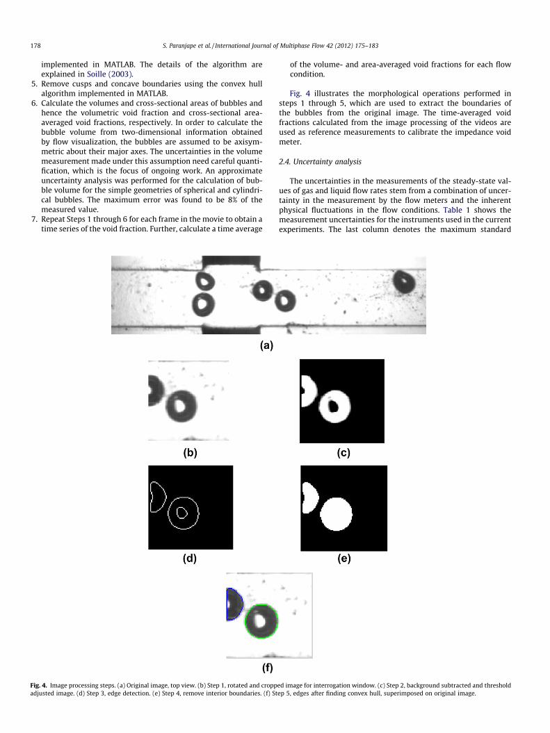
implemented in MATLAB. The details of the algorithm areexplained in Soille (2003).

5. Remove cusps and concave boundaries using the convex hullalgorithm implemented in MATLAB.

6. Calculate the volumes and cross-sectional areas of bubbles andhence the volumetric void fraction and cross-sectional area-averaged void fractions, respectively. In order to calculate thebubble volume from two-dimensional information obtainedby flow visualization, the bubbles are assumed to be axisym-metric about their major axes. The uncertainties in the volumemeasurement made under this assumption need careful quanti-fication, which is the focus of ongoing work. An approximateuncertainty analysis was performed for the calculation of bub-ble volume for the simple geometries of spherical and cylindri-cal bubbles. The maximum error was found to be 8% of themeasured value.

7. Repeat Steps 1 through 6 for each frame in the movie to obtain atime series of the void fraction. Further, calculate a time average

of the volume- and area-averaged void fractions for each flowcondition.

Fig. 4 illustrates the morphological operations performed insteps 1 through 5, which are used to extract the boundaries ofthe bubbles from the original image. The time-averaged voidfractions calculated from the image processing of the videos areused as reference measurements to calibrate the impedance voidmeter.

2.4. Uncertainty analysis

The uncertainties in the measurements of the steady-state val-ues of gas and liquid flow rates stem from a combination of uncer-tainty in the measurement by the flow meters and the inherentphysical fluctuations in the flow conditions. Table 1 shows themeasurement uncertainties for the instruments used in the currentexperiments. The last column denotes the maximum standard

Fig. 4. Image processing steps. (a) Original image, top view. (b) Step 1, rotated and cropped image for interrogation window. (c) Step 2, background subtracted and thresholdadjusted image. (d) Step 3, edge detection. (e) Step 4, remove interior boundaries. (f) Step 5, edges after finding convex hull, superimposed on original image.

178 S. Paranjape et al. / International Journal of Multiphase Flow 42 (2012) 175–183

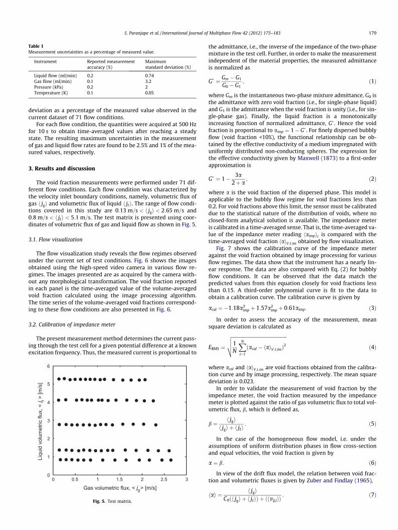
deviation as a percentage of the measured value observed in thecurrent dataset of 71 flow conditions.

For each flow condition, the quantities were acquired at 500 Hzfor 10 s to obtain time-averaged values after reaching a steadystate. The resulting maximum uncertainties in the measurementof gas and liquid flow rates are found to be 2.5% and 1% of the mea-sured values, respectively.

3. Results and discussion

The void fraction measurements were performed under 71 dif-ferent flow conditions. Each flow condition was characterized bythe velocity inlet boundary conditions, namely, volumetric flux ofgas h jgi and volumetric flux of liquid h jf i. The range of flow condi-tions covered in this study are 0:13 m=s < h jgi < 2:65 m=s and0:8 m=s < h jfi < 5:1 m=s. The test matrix is presented using coor-dinates of volumetric flux of gas and liquid flow as shown in Fig. 5.

3.1. Flow visualization

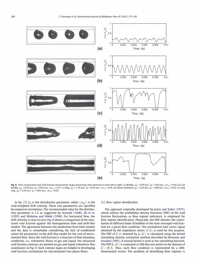
The flow visualization study reveals the flow regimes observedunder the current set of test conditions. Fig. 6 shows the imagesobtained using the high-speed video camera in various flow re-gimes. The images presented are as acquired by the camera with-out any morphological transformation. The void fraction reportedin each panel is the time-averaged value of the volume-averagedvoid fraction calculated using the image processing algorithm.The time series of the volume-averaged void fractions correspond-ing to these flow conditions are also presented in Fig. 6.

3.2. Calibration of impedance meter

The present measurement method determines the current pass-ing through the test cell for a given potential difference at a knownexcitation frequency. Thus, the measured current is proportional to

the admittance, i.e., the inverse of the impedance of the two-phasemixture in the test cell. Further, in order to make the measurementindependent of the material properties, the measured admittanceis normalized as

G� ¼ Gm � G1

G0 � G1; ð1Þ

where Gm is the instantaneous two-phase mixture admittance, G0 isthe admittance with zero void fraction (i.e., for single-phase liquid)and G1 is the admittance when the void fraction is unity (i.e., for sin-gle-phase gas). Finally, the liquid fraction is a monotonicallyincreasing function of normalized admittance, G�. Hence the voidfraction is proportional to aimp ¼ 1� G�. For finely dispersed bubblyflow (void fraction <10%), the functional relationship can be ob-tained by the effective conductivity of a medium impregnated withuniformly distributed non-conducting spheres. The expression forthe effective conductivity given by Maxwell (1873) to a first-orderapproximation is

G� ¼ 1� 3a2þ a

; ð2Þ

where a is the void fraction of the dispersed phase. This model isapplicable to the bubbly flow regime for void fractions less than0.2. For void fractions above this limit, the sensor must be calibrateddue to the statistical nature of the distribution of voids, where noclosed-form analytical solution is available. The impedance meteris calibrated in a time-averaged sense. That is, the time-averaged va-lue of the impedance meter reading haimpit is compared with thetime-averaged void fraction haiV ;t;im obtained by flow visualization.

Fig. 7 shows the calibration curve of the impedance meteragainst the void fraction obtained by image processing for variousflow regimes. The data show that the instrument has a nearly lin-ear response. The data are also compared with Eq. (2) for bubblyflow conditions. It can be observed that the data match thepredicted values from this equation closely for void fractions lessthan 0.15. A third-order polynomial curve is fit to the data toobtain a calibration curve. The calibration curve is given by

acal ¼ �1:18a3imp þ 1:57a2

imp þ 0:61aimp: ð3Þ

In order to assess the accuracy of the measurement, meansquare deviation is calculated as

ERMS ¼

ffiffiffiffiffiffiffiffiffiffiffiffiffiffiffiffiffiffiffiffiffiffiffiffiffiffiffiffiffiffiffiffiffiffiffiffiffiffiffiffiffiffiffiffiffiffiffi1N

XN

i¼1

ðacal � haiV ;t;imÞ2

vuut ð4Þ

where acal and haiV ;t;im are void fractions obtained from the calibra-tion curve and by image processing, respectively. The mean squaredeviation is 0.023.

In order to validate the measurement of void fraction by theimpedance meter, the void fraction measured by the impedancemeter is plotted against the ratio of gas volumetric flux to total vol-umetric flux, b, which is defined as,

b ¼h jgi

h jgi þ h jfi: ð5Þ

In the case of the homogeneous flow model, i.e. under theassumptions of uniform distribution phases in flow cross-sectionand equal velocities, the void fraction is given by

a ¼ b: ð6Þ

In view of the drift flux model, the relation between void frac-tion and volumetric fluxes is given by Zuber and Findlay (1965),

hai ¼h jgi

C0ðh jgi þ h jf iÞ þ hhvg jii: ð7Þ

0 0.5 1 1.5 2 2.5 30

1

2

3

4

5

6

Gas volumetric flux, < jg > [m/s]

Liqu

id v

olum

etric

flux

, < j f >

[m/s

]

Fig. 5. Test matrix.

Table 1Measurement uncertainties as a percentage of measured value.

Instrument Reported measurementaccuracy (%)

Maximumstandard deviation (%)

Liquid flow (ml/min) 0.2 0.74Gas flow (ml/min) 0.1 3.2Pressure (kPa) 0.2 2Temperature (K) 0.1 0.05

S. Paranjape et al. / International Journal of Multiphase Flow 42 (2012) 175–183 179

In Eq. (7), C0 is the distribution parameter, while hhvgjii is thevoid-weighted drift velocity. These two parameters are specifiedby empirical correlations. The recommended value for the distribu-tion parameter is 1.2 as suggested by Armand (1946), Ali et al.(1993) and Mishima and Hibiki (1996). For horizontal flow, thedrift velocity is close to zero. Fig. 8 shows a comparison of the mea-sured void fraction against the homogeneous flow and drift-fluxmodels. The agreement between the predictions from both modelsand the data is remarkable considering the lack of establishedvalues for parameters in the drift flux model for the case of micro-channel flow. Since the void fraction is a function of flow boundaryconditions, i.e., volumetric fluxes of gas and liquid, the measuredvoid fraction contours are plotted on gas and liquid volumetric fluxcoordinates in Fig. 9. Such contour maps are helpful in developingvoid fraction correlations for microchannel two-phase flows.

3.3. Flow regime identification

The approach originally developed by Jones and Zuber (1975),which utilizes the probability density functions (PDF) of the voidfraction fluctuations as flow regime indicators, is employed forflow regime identification. Physically, the PDF denotes the contri-bution of different kinds of bubbles to the time-averaged void frac-tion for a given flow condition. The normalized time series signalobtained by the impedance meter, G�ðtÞ, is used for this purpose.The PDF of G�ðtÞ denoted by fG� ðG�Þ is calculated using the kernelsmoothing density estimation method described by Bowman andAzzalini (1997). A normal kernel is used as the smoothing function.The PDF fG� ðG�Þ is evaluated at 200 discrete points in the domain ofG� 2 ½0;1�. Thus, each flow condition is represented by a 200-dimensional vector. The problem of identifying flow regimes is

0 0.002 0.004 0.006 0.008 0.010

0.5

1

< α

>V [-

]

(a)

0 0.002 0.004 0.006 0.008 0.010

0.5

1

< α

>V [-

]

(b)

0 0.002 0.004 0.006 0.008 0.010

0.5

1

< α

>V [-

]

(c)

0 0.002 0.004 0.006 0.008 0.010

0.5

1

< α

>V [-

]

(d)

0 0.002 0.004 0.006 0.008 0.010

0.5

1

Time, t [s]

< α

>V [-

]

(e)

Time, t [s]

Time, t [s]

Time, t [s]

Time, t [s]

Fig. 6. Flow visualization and void fraction measured by image processing. Flow direction is from left to right. (a) Bubbly, hjgi = 0.29 m/s, hjfi = 0.83 m/s, haiV,t = 0.20. (b) Capbubbly, hjgi = 0.56 m/s, hjfi = 0.83 m/s, haiV,t = 0.37. (c) Slug, hjgi = 1.39 m/s, hjfi = 0.83 m/s, haiV,t = 0.58. (d) Churn-turbulent hjgi = 2.26 m/s, hjfi = 4.08 m/s, haiV,t = 0.36. (e) Longslug, hjgi = 2.65 m/s, hjfi = 0.82 m/s, haiV,t = 0.65.

180 S. Paranjape et al. / International Journal of Multiphase Flow 42 (2012) 175–183

equivalent to identifying clusters of vectors in 200-dimensionalvector space. The clusters of vectors are found by minimizing thedistance between the vectors representing flow conditions and

the weight vectors corresponding to a flow regime. After minimiza-tion, the weight vector positions align with the centroid of theclusters. Thus, the weight vectors that denote the positions of thecluster centroids are characteristic of the flow regime. This optimi-zation problem is solved by the Kohonen Self-Organizing Map algo-rithm for pattern recognition implemented in the Neural NetworkToolbox of MATLAB based on the method developed by Kohonen(1997). Physical interpretation of the recognized patterns isaccomplished by comparing them with the flow regimes observedusing the high-speed camera.

Figs. 10–14 show examples of the impedance meter signals andthe corresponding PDFs obtained for various air–water flow re-gimes. The flow regimes, their qualitative description and charac-teristics of the corresponding impedance meter signals are asfollows. It is noted that stable annular flow could not be achievedwith the current experimental setup.

� Bubbly flow: Bubbly flow is characterized by spherical or ellip-soidal bubbles dispersed in the continuous phase. The majordiameters of these bubbles are smaller than the width of thechannel. The PDF fG� ðG�Þ shows a relatively small width and apeak at higher admittance (Fig. 10).

0 0.2 0.4 0.6 0.8 10

0.1

0.2

0.3

0.4

0.5

0.6

0.7

0.8

0.9

1

Impedance meter measurement, α imp = (1-G*) [-]

Void

frac

tion,

< α

>V,

t,im

[-]

BubblyCap BubblySlugChurn-TurbulentLong SlugPolynomial fitLinearMaxwell (1873)

Fig. 7. Impedance meter calibration.

0 0.2 0.4 0.6 0.8 10

0.2

0.4

0.6

0.8

1

β [-]

Void

Fra

ctio

n, α

[-]

DataHomogeneous FlowDrift Flux

Fig. 8. Comparison of measured void fraction with homogeneous flow and drift-flux models.

0 0.5 1 1.5 2 2.5 30

1

2

3

4

5

6

0.10.2

0.30.4

0.5

0.6

Liqu

id v

olum

etric

flux

, < j f >

[m/s

]

Gas volumetric flux, < jg > [m/s]

Fig. 9. Contours of void fraction.

0 0.002 0.004 0.006 0.008 0.010

0.5

1

G* [-

]

0 0.2 0.4 0.6 0.8 10

10

20

Time, t [s]

Normalized admittance, G* [-]

PDF,

f G* [

-]

Fig. 10. Impedance meter signal and its PDF for Bubbly flow, hjgi = 0.29 m/s,hjfi = 0.83 m/s, haiV,t = 0.20.

0 0.002 0.004 0.006 0.008 0.010

0.5

1

0 0.2 0.4 0.6 0.8 10

5

10

15

Time, t [s]

Normalized admittance, G* [-]

G* [-

]PD

F, f G

* [-]

Fig. 11. Impedance meter signal and its PDF for Cap-Bubbly, hjgi = 0.56 m/s,hjfi = 0.83 m/s, haiV,t = 0.37.

S. Paranjape et al. / International Journal of Multiphase Flow 42 (2012) 175–183 181

� Cap-bubbly flow: As the bubble size increases, it is confined bythe channel walls. It is distorted and forms a cap-shaped bubblewith a round nose at its downstream end. The PDF is character-ized by two distinct peaks located close to each other (Fig 11).The peak corresponding to higher G� represents the liquidregions between the bubbles, while that corresponding to lowerG� represents cap bubbles.� Slug Flow: Long bullet-shaped bubbles are separated by liquid

or small spherical bubbles. The PDF shows two distinct peaks,with one located at low G� corresponding to slug bubbles andthe other located at high G� corresponding to the continuousliquid phase between the slug bubbles (Fig. 12).� Churn-turbulent flow: Due to turbulent agitation at the higher

flow rates, churn-turbulent flow exhibits interacting slug bub-bles with distorted shape. This leads to a wider spread in thePDF, where peaks corresponding to slug bubbles and liquid gapsbetween them are merged. It should be noted here that theexistence of a churn-turbulent regime does not imply highervoid fraction than that in the slug flow regime in a time-aver-aged sense (Fig. 13).� Long slug flow: This regime is characterized by the occurrence of

long stable slugs such that it appears to have a structure similarto annular flow in a local or short-time-averaged sense. The PDFshows a high peak at low G�. Annular flow was not observed inthe current dataset (Fig. 14).

Using the quantitative method of flow regime classification de-scribed above, the dataset was categorized into five regimes. Theresult of this classification is shown in Fig. 15. The flow conditionsare presented on coordinates of volumetric flux of the gas and li-quid phases. The contours of time-averaged void fraction aresuperimposed on the flow regime map. This shows the relationshipbetween flow regime boundaries and the void fraction. This mapcould be used for the development of theoretical flow regimetransition criteria in microchannel two-phase flow.

4. Summary and conclusions

Void fraction is measured in air–water two-phase flowin a microchannel of cross-section 780 lm � 780 lm using acustom-designed impedance void meter. The impedance voidmeter is calibrated against the time-averaged void fraction

0 0.002 0.004 0.006 0.008 0.010

0.5

1

Time, t [s]

0 0.2 0.4 0.6 0.8 10

1

2

3

Normalized admittance, G* [-]

PDF,

f G* [

-] G

* [-]

Fig. 13. Impedance meter signal and its PDF for churn turbulent flow, hjgi = 2.26 m/s, hjfi = 4.08 m/s, haiV,t = 0.36.

0 0.02 0.04 0.06 0.08 0.10

0.5

1

0 0.2 0.4 0.6 0.8 10

2

4

Time, t [s]

Normalized admittance, G* [-]

G* [-

]PD

F, f G

* [-]

Fig. 14. Impedance meter signal and its PDF for long slug, hjgi = 2.65 m/s,hjfi = 0.82 m/s, haiV,t = 0.65.

0 0.5 1 1.5 2 2.5 30

1

2

3

4

5

6

0.1 0.2 0.3 0.4

0.5

0.6

Liqu

id v

olum

etric

flux

, < j f >

[m/s

]

Gas volumetric flux, < jg > [m/s]

Fig. 15. Flow regime map obtained using impedance void meter signals. s: Bubbly,.: Cap bubbly, }: Slug, I: Churn-turbulent, h: Long slug, Level lines: Void fractioncontours.

0 0.02 0.04 0.06 0.08 0.10

0.5

1

0 0.2 0.4 0.6 0.8 10

1

2

3

Time, t [s]

Normalized admittance, G* [-]

G* [-

]PD

F, f G

* [-]

Fig. 12. Impedance meter signal and its PDF for Slug, hjgi = 1.39 m/s, hjfi = 0.83 m/s,haiV,t = 0.58.

182 S. Paranjape et al. / International Journal of Multiphase Flow 42 (2012) 175–183

determined from flow visualization using a high-speed movie cam-era. The calculated time-averaged void fraction shows reasonableagreement with those predicted by the homogeneous flow anddrift flux models. However, a conclusive statement in favor of aparticular model cannot be made since the model parameters(e.g., the distribution parameter and the drift velocity for thedrift-flux model) are not available for microchannel flows.

The probability density function (PDF) of the time series signalobtained by the impedance meter is utilized for quantitative char-acterization of two-phase flow regimes. The flow regimes are iden-tified using a Kohonen Self-organizing map. The present studyshows that the impedance void meter designed in this work canbe used for microchannel two-phase flows for the measurementof void fraction and identification of flow regimes. The void frac-tion and flow regime data obtained by the impedance void metermay be used for developing and benchmarking theoretical flow re-gime transition criteria for microchannel two-phase flows.

Further studies are in progress for extending the flow regimemap to include annular flow, in addition to developing flow regimemaps for additional flow channel geometries. The measurementtechnique developed here can be used to study non-adiabaticand boiling flows with similar geometry of electrodes along withthe same electronic circuit, as long as the changes in electricalproperties of the fluid with temperature are taken into account.

Acknowledgments

This work was funded by the Office of Naval Research (GrantNo. N000141010921). The authors are grateful to Dr. Mark Spectorfor his support.

References

Ali, M.I., Sadatomi, M., Kawaji, M., 1993. Two-phase flow in narrow channelsbetween flat plates. Can. J. Chem. Eng. 71, 657–666.

Andreussi, P., Di Donfrancesco, A., Messia, M., 1988. An impedance method for themeasurement of liquid hold up in two-phase flow. Int. J. Multiphase Flow 14,777–785.

Armand, A.A., 1946. The resistance during the movement of a two-phase system inhorizontal pipes. Izv. Vses. Teplotekh., Inst. 1. pp. 16–23 (AERE-Lib/Trans 828).

Asali, J.C., Hanrtatty, T.J., Andreussi, P., 1985. Interficial drag and film height invertical annular flow. AIChE J. 31, 895–902.

Bertsch, S.S., Groll, E.A., Garimella, S.V., 2008. Review and comparative analysis ofstudies on saturated flow boiling in small channels. NanoscaleMicroscaleThermophys. Eng. 12, 187–227.

Bowman, A.W., Azzalini, A., 1997. Applied Smoothing Techniques for Data Analysis.Oxford University Press, New York.

Coney, M.W.E., 1973. The theory and application of conductance probes for themeasurement of liquid film thickness in two-phase flow. J. Phys. E (ScientificInstruments) 6, 903–911.

Costigan, G., Whalley, P.B., 1997. Slug flow regime identification from dynamic voidfraction measurements in vertical air-water flows. Int. J. Multiphase Flow 23,263–282.

Fossa, M., 1998. Design and performance of a conductance probe for measuring theliquid fraction in two-phase gas-liquid flows. J. Flow Meas. Instrum. 9, 103–109.

Garimella, S.V., Sobhan, C.B., 2003. Transport in microchannles – a critical review.Annu. Rev. Heat Transfer 13, 1–50.

Harirchian, T., Garimella, S.V., 2008. Microchannel size effects on local flow boilingheat transfer to a dielectric fluid. Int. J. Heat Mass Transfer 51, 3724–3735.

Harirchian, T., Garimella, S.V., 2009. Effects of channel dimension, heat flux andmass flux on flow boiling regimes in microchannels. Int. J. Multiphase Flow 35,349–362.

Harirchian, T., Garimella, S.V., 2010. A comprehensive flow regime map formicrochannel flow boiling with quantitative transition criteria. Int. J. HeatMass Transfer 53, 2694–2702.

Hewitt, G.F., 1983. Two-phase flow and its applications: past, present and future.Heat Transfer Eng. 4, 67–79.

Jones Jr., O.C., Zuber, N., 1975. The interrelation between void fraction fluctuationsand flow patterns in two-phase flow. Int. J. Multiphase Flow 2, 273–306.

Julia, J.E., Liu, Y., Paranjape, S., Ishii, M., 2008. Local flow regimes analysis in verticalupward two-phase flow. Nucl. Eng. Des. 238, 156–169.

Kawahara, A., Sadatomi, M., Kumagae, K., 2006. Effects of gas–liquid inlet/mixingconditions on two-phase flow in microchannels. Prog. Multiphase Flow Res. 1,197–203.

Kawahara, A., Sadatomi, M., Nei, K., Matsuo, H., 2009. Experimental study on bubblevelocity, void fraction and pressure drop for gas–liquid two-phase flow in acircular microchannel. Int. J. Heat Fluid Flow 30, 831–841.

Kawaji, M., Kawahara, A., Mori, K., Sadatomi M., Kumagae, K., 2006. Gas–liquidtwophase flow in microchannels: the effects of gas–liquid injection methods.In: Proceedings of the 18th National and Seventh ISHMT–ASME Heat Transfer.

Kohonen, T., 1997. Self-Organizing Maps, Second ed. Springer-Verlag, Berlin.Matsui, G., 1984. Identification of flow regimes in vertical gas-liquid two-phase flow

using differential pressure fluctuations. Int. J. Multiphase Flow 10, 711–720.Maxwell, J.C., 1873. A Treatise on Electricity and Magnetism, third ed. Clarendon

Press, Oxford, England.Mi, Y., Ishii, M., Tsoukalas, L.H., 1998. Vertical two-phase flow identification using

advanced instrumentation and neural networks. Nucl. Eng. Des. 184, 409–420.Mishima, K., Hibiki, T., 1996. Some characteristics of air–water two-phase flow in

small diameter vertical tubes. Int. J. Multiphase Flow 22, 703–712.Serizawa, A., Feng, Z., Kawara, Z., 2002. Two-phase flow in microchannels. Exp.

Thermal Fluid Sci. 26, 703–714.Sobhan, C.B., Garimella, S.V., 2001. A comparative analysis of studies on heat

transfer and fluid flow in microchannels. Microscale Thermophys. Eng. 5, 293–311.

Soille, P., 2003. Morphological Image Processing, second ed. Springer-Verlag,Germany.

The Mathworks Inc., 2009. MATLAB version 2009b.Tsochatzidis, N.A., Karapantios, T.D., Kostoglou, M.V., Karabelas, A.J., 1992. A

conductance method for measuring liquid fraction in pipes and packed beds.Int. J. Multiphase Flow 5, 653–667.

Tumanski, S., 2006. Principles of electrical measurement. CRC Press, Taylor &Francis, USA.

Tutu, N.K., 1982. Pressure fluctuations and flow pattern recognition in vertical twophase gas-liquid flows. Int. J. Multiphase Flow 8, 443–447.

Zuber, N., Findlay, J.A., 1965. Average volumetric concentration in two-phase flowsystems. J. Heat Transfer 87, 453–468.

S. Paranjape et al. / International Journal of Multiphase Flow 42 (2012) 175–183 183