AD-A267 666WL-TR-93-4043 lii I

ELASTIC-PLASTIC FINITE-DIFFERENCE

ANALYSIS OF UNIDIRECTIONAL COMPOSITES

SUBJECTED TO

THERMOMECHANICAL CYCLIC LOADING

Demirkan Coker and Noel E. Ashbaugh

University of Dayton Research Institute300 College ParkDayton, OH 45469-0001 2:

,%%,A UG 0 4 1993' '

December 1992Final Report for 01/01/92-12/01/92

Approved for Public Release; Distribution is Unlimited

Materials DirectorateWright LaboratoryAir Force Materiel CommandWright Patterson AFB OH 45433-7734

\,) 93- 17420 0-. OWN

S..~~~~~. 4.. • a ! i i n

NOTICE

When Government drawings, specifications, or other data are used forany purpose other than in connection with a definitely Government-relatedprocurement, the United States Government incurs no responsibility or anyobligation whatsoever. The fact that the government may have formulated orin any way supplied the said drawings, specifications, or other data, is notto be regarded by implication, or otherwise in any manner construed, aslicensing the holder, or any other person or corporation; or as conveyingany rights or permission to manufacture, use, or sell any patented inventionthat may in any way be related thereto.

This report is releasable to the National Technical Information Service(NTIS). At NTIS, it will be available to the general public, includingforeign nations.

This technical report has been reviewed and is approved for publica-tion.

JAY R. JIRA U ALLAN W. GUNDERSON, ChiefProject Engineer Materials Behavior BranchMaterials Behavior Branch Kctals and Ceramics Division

NORMAN N. GEYERActing Deputy ChiefMetals and Ceramics DivisionMaterials Directorate

If your address has changed, if you wish to be removed from our mailinglist, or if the addressee is no longer employed by your organization pleasenotify WL/MLLN , WPAFB, OH 45433- 7817 to help us maintain a currentmailing list.

Copies of this report should not be returned unless return is required bysecurity considerations, contractual obligations, or notice on a specificdocument.

Form ApprovedREPORT DOCUMENTATION PAGE OMB No. 0704-0188

Public reportinq burden for this collection of information S est i ated to average I hour per reponse including the time for rev.ewving nstruct,ons. searchinq exsting data sources.latherinq and maintaining the data needed, and (ompletinq and reviewing the collection ot information Send comments re•arding this burden estimate or an0 other &aspect of thincollection of inftormatiOn, including suggestions for reaucing this burden to Washington Headcluarters Services. Directorate for Innfirm tion Operations and Reports. 1215 JetferwnDavis H4qhwav. Suite 1204. Arlington. VA 12202-4302. And to the Office of Managernent and Budget. Paperwork Redurtlon Project (0704-0188). Washington. DC 20503

1. AGENCY USE ONLY (Leave blank) 2. REPORT DATE 3. REPORT TYPE AND DATES COVERED

December 1992 Interim: January 1992-December 19924. TITLE AND SUBTITLE 5. FUNDING NUMBERS

Elastic-Plastic Finite-Difference Analysis of F33615-91-C-5606Unidirectional Composites Subjected to Thermomechanical PE-61102Cyclic Loading PR-2302

6. AUTHOR(S) TA- P1Demirkan Coker and Noel E. Ashbaugh WU-03

7. PERFORMING ORGANIZATION NAME(S) AND ADDRESS(ES) 8. PERFORMING ORGANIZATION

University of Dayton Research Institute REPORT NUMBER

300 College ParkDayton, OH 45469-0001

9. SPONSORING / MONITORING AGENCY NAME(S) AND ADDRESS(ES) 10. SPONSORING / MONITORING

Materials Directorate AGENCY REPORT NUMBER

Wright Laboratory WL-TR-93-4043Air Force Materiel CommandWright-Patterson Air Force Base, OH 45433-7734

11. SUPPLEMENTARY NOTES

12a. DISTRIBUTION/ AVAILABILITY STATEMENT 12b. DISTRIBUTION CODE

Approved for public release; distribution is unlimited.

13. ABSTRACT (Maximum 200 words)

An analytical tool was developed to model a unidirectional composite subjected tothermomechanical cyclic loading and processing conditions. The finite difference method wasincorporated into a PC compatible computer code, FIDEP (Finite-Difference Code for Elastic-PlasticAnalysis of Composites). FIDEP provides an efficient numerical procedure for analyzing a variety ofproblems involving thermal and mechanical cycling. The procedure allows the modeling of theconstituent materials as elastic-plastic with temperature dependent properties. The concentric cylinderapproximation allows the computations to capture the three-dimensional aspects of the stress state ina real composite. Results for a thermal cool-down in an SCS-6/ITi-24AI-1 1 Nb unidirectional compositecompare well with those obtained using the finite element method. Several problems were solved forthermomechanical loading conditions and demonstrate the three-dimensional nature of the stress fieldsin the matrix material.

14. SUBJECT TERMS 15. NUMBER OF PAGES90

Concentric cylinder model, e'astic plastic, finite difference methods, metal 16. PRICE CODEmatrix composite, thermomechanical fatigue, unidirectional composite.

17. SECURITY CLASSIFICATION 18. SECURITY CLASSIFICATION 19. SECURITY CLASSIFICATION 20. LIMITATION OF ABSTRACTOF REPORT OF THIS PAGE OF ABSTRACT

Unclassified Unclassified Unclassified UL

NSN 7540-01-280-5500 Standard Form 298 (Rev 2-89)Pter,bied by ANSI Sfd 139-18248-102

TABLE OF CONTENTS

LIST O F FIG U R ES ........................................................................................................ v

LIST O F T ABLES ......................................................................................................... vii

FO R EW O R D ................................................................................................................ viii

1. IN T R O D U CTIO N ................................................................................................... 1

2. BA C K G R O U N D ..................................................................................................... 2

3. T H EO R Y .......................................................................................................... 4

3.1 Concentric Cylinder M odel .................................................................... 43.2 G overning Equations ........................................................................... 4

3.3 Com putation of Axial Strain ................................................................... 73.4 Finite D ifference Form ulation ................................................................ 9

3.5 Plasticity Theory .................................................................................... 133.5.1 Prandtl-Reuss Relations ............................................................ 13

3.5.2 Plastic Strain-Total Strain Plasticity Equations ........................ 15

3.6 Solution Technique ................................................................................ 18

4. IM PLEM ENTATIO N IN FID EP ...................................................................... 21

4.1 A lgorithm ............................................................................................ 214.2 Faster Convergence Schem e ................................................................. 25

5. PR O G R A M ........................................................................................................... 27

5.1 G eneral D escription ............................................................................ 275.2 Program O peration ............................................................................. 27

5.2.1 Input ........................................................................................ 285.2.2 O utput ...................................................................................... 28

!iii

5.2 .3 P rogram 3........................................................................................ 325.2.4 Execution of FIDEP on a VAX/VMS Machine .............................. 32

6. DEMONSTRATION PROBLEMS ..................................................................... 34

6.1 M aterial Properties ............................................................................... 34

6.2 Comparison with Elastic Solution .......................................................... 34

6.3 Comparison with Finite Element Method ............................................ 38

6.3.1 Cool-Down from Processing Temperature .............................. 38

6.3.2 Cyclic Loading .......................................................................... 45

6.4 Thermo-Mechanical Fatigue (TMF) ...................................................... 48

R E F E R E N C E S ........................................................................................................ 57

APPENDIX 1. LISTING OF FIDEP SOURCE CODE .................................. 60

APPENDIX 2. ELASTIC SOLUTION OF TWO CONCENI'RIC

C Y LIN D ER S ........................................................................... 84

APPENDIX 3. SAMPLE OUTPUT FILES .................................................... 85

\ tW,

i x

yIC QTILrry TNSf PC"D 21

iv

LIST OF FIGURES

Figure 3.1 Concentric Cylinder Idealization of a Unidirectional Composite andthe Concentric Cylinder M odel ................................................................ 5

Figure 3.2 Discretization of the Concentric Cylinder Model ...................... 10

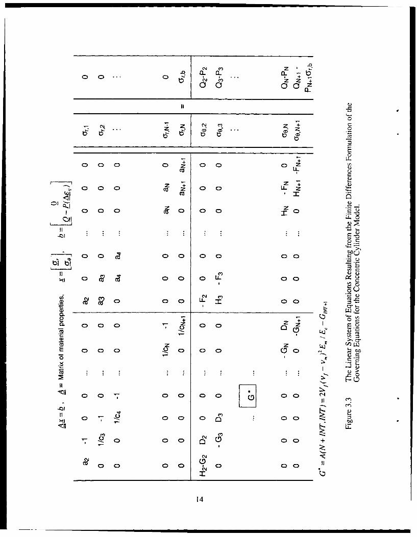
Figure 3.3 The Linear System of Equations Resulting from the FiniteDifferences Formulation of the Governing Equations for tiheConcentric Cylinder M odel ................................................................... 14

Figure 3.4 Schematic of the Iterative Technique for Computing Plastic StrainsUsing the Prandtl-Reuss Relations ........................................................ 19

Figure 3.5 Schematic of the Iterative Technique for Computing Plastic StrainsUsing the Modified Prandtl-Reuss Relations ......................... 19

Figure 4.1 Elastic-Plastic Algorithm Used in FIDEP ............................................. 22

Figure 4.2 Pseudo-Code for the Computer Program FIDEP ................................. 23

Figure 4.3 Schematic for the Computation of a New Estimate for the PlasticStrains Using the Previous Estimates and their Differences .................. 26

Figure 5.1 Example Loading History Input File, FDLOAD.DAT ........................... 29

Figure 5.2 Example Material Properties Input File, FDMAT.DAT ......................... 29

Figure 5.3 Example Command File for Running Batch Jobs on a VAX/VMSCom puter System .................................................................................. 33

Figure 6.1 Variation of Elastic Stresses with Radius Obtained by ElasticClosed-Form Solution and FIDEP for AT=-100°C ............................... 36

Figure 6.2 Elastic and Elastic-Plastic Predictions of Stresses at a Cross-Sectionof the Composite after Cool-Down from the Processing Temperatureo f 10 10,C ............................................................................................ . . 37

Figure 6.3 a) Loading Input File, and b) Schematic of the Temperature Historyfor a Thermal Cool-Down Simulation of SCS-6/Ti-24AI- 11 NbUnidirectional Composite ........................................ 39

Figure 6.4 Finite Element Model and the Boundary Conditions for anAxisymmetric Concentric Cylinder Geometry Under GeneralizedPlane Strain Condition ........................................................................... 40

Figure 6.5 Finite Element and FIDEP Predictions for the Stresses at theInterface in Ti-24A1- II Nb Matrix after Cool-Down from ProcessingTem perature of 1010°C .......................................................................... 41

V

Figure 6.6 Finite Element and FIDEP Predictions for the Plastic Strains at theInterface in Ti-24A1-1 1Nb Matrix after Cool-Down from ProcessingTem perature of 1010'C .......................................................................... 42

Figure 6.7 Variation of the Stresses Across the Cross-Section of the CCMAfter Cool-Down from Processing Temperature of 1010°C .................. 43

Figure 6.8 Variation of the Plastic Strains Across the Cross-Section of theCCM After Cool-Down from Processing Temperature of 1010°C ........ 44

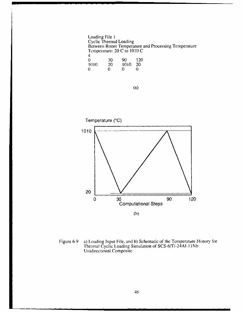
Figure 6.9 a) Loading Input File, and b) Schematic of the Temperature Historyfor Thermal Cyclic Loading Simulation of SCS-6/Ti-24A1-I 1NbU ndirectional Com posite ....................................................................... 46

Figure 6.10 FIDEP and FEM Predictions for the Effective and Radial Stresses inthe Matrix at the Fiber-Matrix Interface for Thermal LoadingH istory show n in Fig. 6.9 ..................................................................... 47

Figure 6.11 a) Loading Input Files, and b) Schematic of the Temperature andStress History for Typical In-Phase and Out-of-Phase TMF Cycles,.......... 49

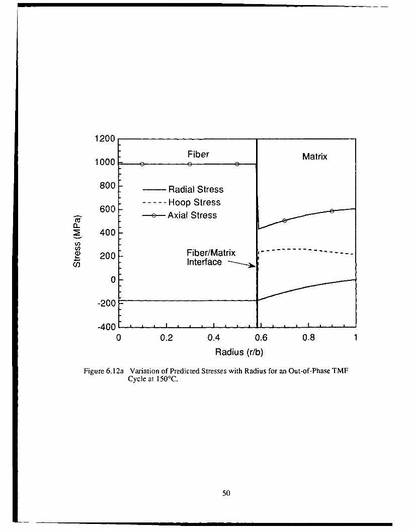
Figure 6.12a Variation of Predicted Stresses with Radius for an Out-of-PhaseTM F Cycle at 150'C ............................................................................. 50

Figure 6.12b Variation of Predicted Stresses with Radius for an Out-of-PhaseTM F C ycle at 650'C ............................................................................. 51

Figure 6.13 Axial Stress Predictions in the Ti-24A1- 11 Nb Matrix at the Fiber-Matrix Interface for In-Phase and Out-of-Phase TMF CyclicL oading ............................................................................................... . . 53

Figure 6.14 Axial Stress Peaks Predicted in the SCS-6 Fiber for In-Phase andOut-of-Phase TMF Cyclic Loading ....................................................... 54

Figure 6.15 Radial and Hoop Stress Predictions in Ti-24AI-1 1Nb Matrix at theFiber-Matrix Interface in TMF Cyclic Loading ...................................... 55

v;

LIST OF TABLES

Table 5.1 Format for the Input Loading File, FDLOADDAT ..................................... 30

Table 5.2 Format for the Material Properties File, FDMAT.DAT ............................... 30

Table 6.1 Mechanical Properties for SCS-6 Fiber and Ti-24AI- I I Nb Nlatrix ............ 35

V11

FOREWORD

This report documents a computer program that was developed as part of an investigation of

the mechanical behavior of metal matrix composites. The investigators were Demirkan

Coker and Noel E. Ashbaugh of the Structural Integrity Division, University of DaytonResearch Institute, Dayton OH. The research was conducted at the Materials BehaviorBranch, Metals and Ceramics Division, Materials Directorate, Wright Laboratory

(WL/MLLN) Wright-Patterson AFB OH, under Contract No. F33615-91-C-5606. The

contract was administered under the direction of WL/MLLN by Mr. Jay R. Jira. Dr. Noel

E. Ashbaugh was the Principal Investigator and Dr. Joseph P. Gallagher was the Program

Manager.

viii

CHAPTER IINTRODUCTION

Interest in metal matrix composites (MMC) for high-temperature aerospace

applications has grown in recent years. Because of the high use temperatures envisioned,

proposed applications of MMCs almost always involve both thermal and mechanical cyclic

loading. Consequently, the accurate prediction of the thermornechanical fatigue (TMF) life

of these components is a critical aspect of the design process. Because of the mismatch in

coefficient of thermal expansion between fiber and matrix, internal thermal stresses are

produced during cool-down from the processing temperature and subsequent thermalcycling. These stresses must be accounted for in the analysis in addition to those produced

by mechanical loading. Prediction of the mechanical behavior and life of a composite

material, therefore, requires a knowledge of the individual components of -:ress or strain in

the fiber and/or matrix as well as the overall applied stresses.

In this investigation, an axisymmetric concentric cylinder geometry was used to

model the unidiredtional composite in which the fiber and matrix were represented by the

core cylinder and outer cylinder, respectively. The concentric cylinder geometry allowed for

a relatively simplified analysis and was adequate for predicting the complex three-

dimensional stress distributions in the fiber and the matrix. The analysis allowed for axial

and radial loading and more than two constituents with bilinear elastic-plastic properties.The analysis also accounted for thermomechanical loading and temperature dependent

material properties. These aspects were incorporated into a FORTRAN program, FIDEP

(Finite Difference Code for Elastic-Plastic Analysis).

This report summarizes the derivation and application of the concentric cylindermodel to predict the micromechanical stresses in an SCS-6/Ti-24AI- 11 Nb metal matrix

composite. The next chapter summarizes some of the past work done on micromechanical

modeling of composites. Chapter 3 describes the theory for the concentric cylinder model

and summarizes plasticity theory. In Chapter 4 the implementation of the theory to thecomputer program, FIDEP, is described and the procedures for using this program are

explained in Chapter 5. Finally some example runs are conducted with this program and

the results are presented.

CHAPTER 2BACKGROUND

Various ap1,.aches have been adopted in the past to calculate the micromechanicalstresses in the fiber and the matrix due to both thermal and mechanical loading. The mostwidespread approach involves use of the finite element method to model a representativevk,, .me element (RVE) and compute the stress distributions around the fiber. CommonRVE geometries that have been used include either a square or a cylindrical fiber in a squarematrix and a cylindrical fiber in a cylindrical matrix. Different constitutive behaviorsinclude elastic-plastic behavior [1-31, time-dependent behavior using a classical creep law

141 and unified viscoplastic theories such as the Bodner-Partom model [5), and Bodner-Partom with backstress 161. However, finite element codes are sually run on mainframecomputers, are time consuming, allow for solution of only one problem at a time, andrequire familiarity with finite element analysis and the code. To conduct a parametric studyand to support the design of a large number of experiments on different composite systems,a more practical approach is desirable.

One simple approach to micromechanical modeling of composites has been to useaverage stresses in the constituents. This method has the advantage of being easy toimplement into a code and of easily being extended to analyze laminates. Approaches usingthis method include analysis of square fiber in a square matrix and the vanishing fiberdiameter (VFD) model developed by Dvorak and Bahei-E1-Din [71. In the VFD model, thepresence of the fibers is assumed not to influence the transverse stresses. The transverseproperties of a zamina are easily computed using this assumption while the longitudinalproperties are calculated from the rule of mixtures. This analysis can be carried out for anelastic fiber surrounded by a matrix material having a variety of constitutive relations tocalculate ply properties which, in turn, can be incorporated into lamination theory to analyzea composite. Such a procedure has been implemented into computer codes such asAGLPLY 181 which uses thermoplastic matrix behavior and VISCOPLY 191 whichincorporates the Eisenberg creep model to predict average stresses in the constituents and ina symmetric composite laminate subjected to thermomechanical loading. Aboudi I101modeled a square fiber in a square matrix subcell using first order displacement expansions.The unified theory of Bodner and Partom was used to compute inelastic strains. Hopkins

and Chamis (111 and Sun 1 121 conducted strength-of-materials type analyses for a squarefiber in a square matrix cell to obtain expressions for the constituent microstresses. Chamis

2

and Hopkins 1131 modified these expressions based on exneiimental data for uniaxial

lamina and three-dimensional computer simulations of composite behavior. The results

were incorporated into a computer program, METCAN [141, which treats material

nonlinearity at the constituent level where material behavior is modeled using a time-

temperature-stress dependence of constituent properties.

The main drawback to all of these simplified material models is the assumption of

average uniform stress in the representative volume element. This apprc;-ach fails to take into

account the triaxial stresses that arise due to the mismatch of the Poisson's ratio and the

coefficient of thermal expansion of the constituents. A detailed review of these codes and

comparisons of the stresses using these methods and using finite element analysis is given

by Bigelow et al. [ 15].

For a more accurate analytical treatment of the triaxial stresses, the concentric

cylinder model has been used in the literature due to its simple geometry. Thermoelastic

treatment of the axisymmetric concentric cylinder model with multiple rings are given in

references [16, 171. An elastic analysis of a multidirectional coated continuous fiber

composite by means of a three-phase concentric cylinder model is given in reference [18].

Ebert et al. [19] and Hecker et al. [20] were the first to introduce elastic-plastic behavior for

the constituents in which they modeled two concentric cylinders and verified the model with

experiments. Gdoutos et al. used this model to compute thermal expansion coefficients

1211 and stress-strain curves and obtained good agreement with experimental results [221.

However, this approach postulated new stress-strain relations in which the strain increments

were functions of the stress increment, in contrast to the Pranatl-Reuss relations that relate

the strain increments to the current state of stress. This method is a deformation type of

theory and could not be applied to nonproportional loadings and ideally plastic material.

More recently Lee and Allen [231 obtained an analytical solution for elastic-perfectly plastic

fiber and matrix obeying Tresca's yield criterion.

In this investigation an analytical tool was developed to compute the three-

dimensional stress state in a composite using the concentric cylinder model. The analysis

accommodates multiple materials having elastic-plastic behavior with strain hardening. The

PrandtI-Reuss flow rule with the von Mises yield criterion was used. In addition,

temperature-dependent material properties were taken into account. The analysis was

implemented into the computer code FIDEP (Finite Difference Code for Elastic-Plastic

Analysis of Composites) which accounts for thermomechanical cyclic loading.

3

CHAPTER 3THEORY

The derivations of the elastic-plastic concentric cylinder equations are described inthis section. The solution technique for the numerical integration of the Prandtl-Reuss

equations are also summarized.

3.1 Concentric Cylinder Model

A representative volume element of the composite is modeled as concentric cylinderswith the core cylinder representing the fiber and the outer ring representing the matrix (Fig.

3.1). The fiber and matrix radii are denoted as a and b, respectively. The direction of the z-axis is along the fibers and the cylinders are infinitely long in the axial direction.

Cylindrical coordinates are used in the equations.

The following assumptions are made in the analysis. The temperature distribution is

uniform and is quasi-static. A perfect bond exists between the constituents of the composite

so that there is no slippage or separation of the constituents. The concentric cylinders are in

generalized plane strain and are subjected to axisymmetric loadings and displacements sothat the shear stresses are zero. The constituent properties are isotropic. The fiber is

linearly elastic. The matrix follows a von Mises yield surface and is incompressible in the

plastic region, i.e., hydrostatic stresses do not cause plastic deformation. The plastic

deformation of the matrix is governed by the Prandtl-Reuss flow rule.

The following boundary conditions are imposed:1) radial stress is Pr at r=b,

2) finite stresses at r=O, and

3) continuous radial displacements and radial stresses at the interface.

3.2 Governing Equations

Equilibrium and compatibility equations in tcylindrical coordinates for an

axisymmetric generalized-plane strain case simplify to 1241:

.... e .....

0g*be r

"............. ......

hr

Fig. 3.1I Concentric Cylinder Idealization of a Unidirectional Composite andthe Concentric Cylinder Model.

5

d o ', + 0, - a g- 0U -- =0, (1)

dr r

dee E,- o= 0 , (2)

dr r

and the stress-strain equations are (25]:

1

1

E= -I(ao - v(Or + a,))+ aT+c E+deE, (3)E E

e

= -(a - v(Oa + y6 )) + aT + de+ 'E

where ErP, e0P and czP are the total accumulated plastic strains up to, but not including the

current increment of loading, d~rP, dE0P and dczP are the plastic strain increments due to the

current increment of loading, Er, Eo and ez are the total strains, Or, c0 and az are the stresses,

(x is the secant coefficient of thermal expansion (CTE), v is the Poisson's ratio, E is the

Young's modulus and T is the change in temperature from a reference state in which the

stresses and the strains are assumed to be zero.

Substitution of Eqn. 3 into Eqn. 2 to eliminate total radial and hoop strains yields:

d( _ v (a,+ V(U,.+a.) - aET + E(e.-e- de))+ aT+e +deP)dr E E

(I+ v) +•deP -ef -dePEr +0 (4)

This equation together with the equilibrium equation results in two ordinary differential

equations in the two unknowns, Or and 00. The axial strain, EZ, is a constant value across the

cross section because of the imposed generalized plane strain condition.

6

3.3 Computation of the Axial Strain

To compute the axial strain, the stress-strain equation in the axial direction (Eqn. 3)

is multiplied by E r and integrated over the cross section:

b b b b b

ejErdr= Jardr-v(ar, + a8)rdr+JaETrdr+JE(ef +de)rdr. (5)0 0 0 0 0

For k concentric cylinders, let ai be the outer radius of the ith ring and ao = 0, then the

integral on the left hand side reduces to:

b k Ee, f Erdr= eI '-(a' - a,). (6)

0 iz '1 2

The first integral on the right hand side is evaluated using the global equilibrium equation in

the axial direction; i. e. internal forces are equal to the external applied forces:

b

f a,(2 rr)dr = P,(7rr2 ), (7)0

where Pz is the applied axial stress.

Rearranging the terms, the equilibrium equation (Eqn. 1) can also be written as [26]:

(a, + c76)r = d (r2 r). (8)dr

Using Eqn. 8, the second integral on the right hand side of Eqn. 5 becomes:

v - (r r,.) dr= vi ,(a g, r(a,) - cr,_ (a,_1) 90 s=1

Expanding and recollectirg terms in Eqn. 9:

b d 2 k-1

Jv-(r a,)dr = X(Vi - V5 i)aIar(a,) + v, ba, (b), (10)0 dr

7

where Or(b) is the applied radial stress at r=b.

The remaining terms are similarly evaluated assuming constant material properties

and temperature distribution in each cylinder. The axial strain for k concentric cylinders

then becomes:

1 { k-i

--• P,= - 21_Va,(a,)(v, - v,,,)-2vcr,(O)+ oET

Sb (11)~~E XEJe d~)rdr1

where, Vi is the volume fraction of the ith cylinder, Ec is the axial composite modulus and

etc is the axial coefficient of thermal expansion of the composite defined by:

2 2

k

a=Z, -a,

andk

c E ,

In the case of two concentric cylinders representing an elastic fiber and an elastic-plasticmatrix, k = 2 and EzP = 0 in the fiber, so that the expression for the axial strain simplifies to:

22 E.Ez= P, -2V, (v - v,,)c,(a)- 2 vP, + acEcT+ b----(e+deP)rdr ,(12)

where ac I •(of EfVf + a•. E. V.)

Ec =VE+ E,,+E.V.,

8

and Vf and Vm are the fiber and matrix volume fractions, respectively, and Pr is the applied

radial stress at r=b. In Eqs. 11 and 12, the axial strain is written in terms of the radial

stresses at the interfaces. The total plastic strains are known from the previous loading

steps and the new plastic strain increments are related to the stresses through the Prandtl-

Reuss flow rule.

Note that if the Poisson's ratio for the cylinders is the same and the applicd radial stress is

zero, the second and third terms vanish leaving the total axial strain as the sum of the

composite elastic strain (ezCc), composite thermal strain (Azthc) and composite plastic strain(&,,Pc), i. e.:

cc the P Z =_ + 2 E,,'rpJ

If the plastic strain is constant throughout the matrix, then we have for the total strain:

EZ = P + oT + .EV e ,EP E, E z

where EPr is the average matrix plastic strain.

3.4 Finite Difference Formulation

The method of finite differences is used to solve the two ordinary differential

equations [251. The disk radius is divided into N intervals as shown in Fig. 3.2. There are

thus N+1 stations, the first station being at the center of the disk and the last station at the

outer radius. Eqs. I and 4 are written in finite difference form at midpoints of these

intervals as follows:

ri - r,,_ d ar,.E -a0, 1-EI2-- 2 'rr - r, -r,_

cyr. " - 2 - 2 1 ' "d (a, CFO', I_ r - r _ 9

9

z

Ia Fibe/MarixberIx Interface:

Fig.3.2Diretzaton f the Concetric ClinerMoel

10

Sv)1- = 1 t(1+ v, )o.,/E, -(1+ v,_,)a 0 .,_/E,_,V) - etc.rliy 2 ri - ri_1 /2

In this manner Eqs. 1 and 4 can be written at the midpoints of n stations resulting in 2n

equations;

1-r.j1- - 6, + aiji-i +a- a 8oj == 0cir + =2... -1, (13)

Gjoi.,_j + DiOr.i + HnU,._j - Fxcro., = Q, - P,

where

ai = (ri - r,-,) / 2r, , bi = E j / E,_j , c, ri I ri_-,

and

D = (1 + v,)( + a),

Fj = (1 + vy)(1 - v1 + aj)

Gi = bi (I + vi-1)(vi_1 - aici),

Hi = bi (I + vi-I )(I1- vi-I - aici),

Qj = ET(oai(I + v,) - aj_(1 + v,-,)) ,

Pi = Ej(P: + e,(vi - vi- 1))

Pi=V(Cp++ p+ p+-P•= vje%+ eg, )- v,_('e.,_ + eo.,)

± , +cE (/a 1 +1) + "(++a, EP; i eP._ - +1a + o,-,_(l( a, - c,)]

where the plastic strains, er+, etc., are the updated plastic strains, i. e. E -=,, + deP etc.

The coefficients at the left hand side are functions of material properties at the ith station.Only the P* term on the right hand side involves plastic strains. The unknowns are nr,i anda0,j, i = 1,...,n+l. Using the boundary conditions, ar,n+1 = Pr and o0,1 = Gr,l, the

I1

unknowns reduce to 2n; ar,i, i=l,...,n, and 00,i, i=2,...,n+l. The axial stress distribution, o5,j,

i= 1,...,n+l, is given by Eqn. 3.

Moving the radial stress terms in Eqn. II to the left hand side of Eqn. 13 and letting

the radial stress at the jth interface correspond to the radial stress at node i=Ij, i. e.,r,, (a,) = o./ , the second expression in Eqs. 13 becomes:

-Giari-l + Diar.j + Hico i-I - Fiuo'i - 2(vi - Vi-()E-1V, - 11+)- i, (14)

=Q, - E.,.' - E, (y, - v,_,)E:

where

2 k b P= (P2-PE +2 b YE fe rdr). (15)j=1 0

In the ::se Lf two concentric cylinders, k=2 and j=l. Let INT be defined as the index of thehighest-numbered node in the fiber and INT+1 be the index of the lowest-numbered node

in the matrix. The fiber-matrix interface lies between these two nodes. Then, for all

equations in which i * INT+1, i. e., equations for nodes not adjacent to the interface, ni-ni-I

is zero and the axial strain vanishes from these equations. For the INT+lst equation, Eqn.

14 reduces to:

( 2 Vf E, / E: (v - V.) 2 - Gm+)ar.i),.1

+DrTm+l fNr~t + HImN+, ao~mr + FJNT+1 6OINT+I. (16)

= Qwi- EmPm.+- E.(vm - v)e;

One final step before Eqs. 13 are written in matrix form is to eliminate singular terms for

i=2. Note that (Yr,1 = 50,1. Thus ar,1 and 00,1 terms can be combined in Eqn. 13 to obtain:

(1/c 2 + a2 ) 1 r- 47, 2 + a 2 470, 2 = 0

(H2 -G 2 )ar,Q + D2 ar,2 - F2a9 ,2 = Q2 - P2

In the first equation 1/c2 = rI/r2 = 0. In the second equation, the term H2-G 2 is expanded

and simplified. The final equations for i=2 become:

12

a2,.l -- (r.2 + a 2 6,e 2 ' 0

(1 + "'. )(1 - 2v,)b 2 4g,. +D 2 Cr, 2 -F 2 'gO, 2 = Q2 - P2

Hence Eqn. 13 is written in matrix form as:

Ax=B, (17)

where A is a 2n by 2n matrix of constant coefficients, x is the radial and hoop stress vector

of length 2n and B is a vector of length 2n, as shown in Fig. 3.3. In matrices A and B all

the constants are known except the plastic strain increments which are presumed or

computed from the Prandtl-Reuss relations.

3.5 Plasticity Theory

The plastic strains increments are computed using Prandtl-Reuss relations [25]. In

this section two forms of the Prandtl-Reuss equations are summarized; equations relating

plastic strain increments to stresses and equations relating plastic strain increments to

modified total strains.

3.5.1 Prandtl-Reuss Relations

Prandtl and Reuss assumed that the plastic strain increment is proportional to the

instantaneous stress deviation, i. e.:

deP = XS,1 (18)

where Sij is the deviatoric stress tensor and ?L is a nonnegative constant which may vary

throughout the loading history. These equations imply that the plastic strain increments

depend on the current stress state and not on the stress incremt~nt required to reach thisstate. To determine k, both sides are squared and multiplied by 2/3 to obtain:

2 .2 L2SjS (19)3 11 3

Define effective plastic strain increment and effective stress, respectively, as:

13

Co, 0 . .q c a. a. q~0 ~~0 0 Z IS

C z C\! Cli z z+00 00 ID

o0 CD C z C) :

cu L)

++

o0 0 0 0 C 0 u

C:V

0 C0) 0 0 IL z

0f 0) 0 0 0- 0 10

A? Cu

4)) 0_

2 + +- 0D 0 0D 0 > 0 C~z

z U>

X E

00 Cl 0> 0 0 0 00 C

0> 'ý 0 0 C).

C) ' 0D 00 ) 00C

Cj

8U 0 0) 0) 0) 0 00 (

14

deP = 2d~e and uf :- ýsij (20)

Using these definitions ), is determined from Eqn. 20 as:

3 deP (21)2 04

and the Prandtl-Reuss relations become:

de, -o 3 deP Sj. (22)

These equations are used together with the von Mises yield criterion. Yielding begins when

the effective stress reaches the yield stress determined from a uniaxial tensile test.

3.5.2 Plastic Strain-Total Strain Plasticity Relations

The above form of the Prandtl-Reuss relations relate the plastic strain increments to

the stresses. Another method to computing the plastic strain increments is to use equations

that relate the plastic strain increments to the modified total strains. These equations will be

more stable with respect to the loading increment size and converge faster for most loading

cases. In this approach the plastic strain increments are computed using modified Prandtl-

Reuss relations derived by Mendelson [25].

Assume a loading path to a given state of stress and total plastic strains CijP and let

the next load step be applied producing additional plastic strains AEijP. The total strains can

be written as:

E= + E+A , (23)

where cjf is the elastic component of the total strain, eijth is the thermal strain, ,ijP is theaccumulated plastic strain up to (but not including) the current increment of load, and AEijP

is the increment of plastic strain due to the increment of load. The previous plastic strains

'ijP are presumed to be known, and AeijP is to be calculated.

15

'ile modified total strains are defined as:

cE, -, + AEf. (24)

The deviatoric strains are obtained by subtracting the mean strain from the diagonal

compoe ent of both sides:

e,, = e + AeP. (25)

where Eije is the elastic strain deviator tensor and eij' is the modified strain deviator tensor.

From Hooke's Law and Prandtl-Reuss Eqn. 18:

S.j Ae,(

2G-- 2GA'

where G is the shear moduits. Using this expression and Eqn. 18, Eqn. 25 becomes:

e = (I + 2- )de,,Pe'

2GA

Multiplying both sides of the equation by two thirds itself:

2e ,e, 2 (1 + 2-)2de~deP'.

3 " 3 2GA. "

Define effective modified total strain in a similar fashion to the effective incremental plastic

strain rate to obtain:

e = (I + )deP. '27)2 GA

The modified Prandtl-Reuss relations then become:

depde, =:ee' ,, (28)

e,1

16

where cij' are the modified total deviatoric strains, e',ff is the equivalent or effective modified

total strain defined by:

e 3 U e'ed, (29)

and dcp is the equivalent or effective plastic strain increment defined by Eqn. 20. The

modified Prandtl-Reuss equations in expanded form are:

dePde-= =d (2e'-e';-e;),

S= - (2E' -c' -e'),3e'eff

dep, = 'f- (2e' -e' -e') = -(de + de)

dale = e4 e' dcP= -- e', de= e

Equation 28 is equivalent to the Prandtl-Reuss Eqn. 18, but relate the incremental plastic

strains to modified total strains instead of the stresses.

The relationship between the effective incremental plastic strain and effective

modified total strain is obtained by substituting X from Eqn. 21 in Eqn. 27:

,if = "' + I ,Y" (30)

Let the effective stress from the previous loading step be ,.._i. By expanding the effective

stress in a Taylor series about ad -8_1:

( deP ), _, "

the effective stress is eliminated from Eqn. 30 to obtain:

17

d C:ff 3 G ef31)deS = 3G(31 )

l+ (da.f / )&_,

The effective modified total strain has no physical significance and is purely a mathematicalquantity even in the uniaxial case. In Eqn. 31 a small error in effective modified total strainor the effective stress will produce the same order-of-magnitude error in the effective plasticstrain increment since the denominator is approximately unity. Equations 28, 29 and 31 areused simultaneously to determine plastic strain increments at each loading step.

3.6 Solution Technique

Solution of the elastic-plastic concentric cylinder problem requires the solution of 5equations; the equilibrium and compatibility Eqs. I and 6, and the three Prandtl-Reussrelations (Eqn. 22 or 28). After elimination of the strains using the constitutive relationsthere are 6 unknowns left; Or, YO, Oz, derp, deop, dEzp. The axial stress is eliminated usingEqn. 11 reducing the number of unknowns to 5. The ordinary differential equations (Eqs. 1and 6) are solved using the method of central finite differences to obtain a linear system ofequations (Eqn. 13). These simultaneous equations are used in an iterative plasticityalgorithm to solve for the stresses.

There are two iterative algorithms that were considered for this investigation both ofwhich use forward-Euler integration scheme. The first algorithm uses the Prandtl-Reussrelations (Fig. 3.4). For an increment of load, a distribution is assumed for the plastic strainincrements. The finite difference equations are then solved for a first elastic approximation

to the stresses and strains. At the same time, the effective plastic strain increment iscalculated (Eqn. 20). From the stress-strain curve the ciirt,,jnding effective stress iscomputed. Finally, a new estimate computed for the pli' '- m increments and thesesteps are repeated until convergence is obtained. Th" .. -;n is not a very stablealgorithm and may not converge for large load increments.

The second iterative method uses the modified version of the Prandtl-Reuss Eqn. 28or the plastic strain-total strain relations developed by Mendelson (251. This method is alsocalled the elastic-predictor radial corrector method. In this algorithm (Fig. 3.5), total strainsare obtained from the stresses from Eqn. 13 with assumed or previously calculated plastic

18

A0e.. < : O..E 14 1p

Figure 3.4 Schematic of the Iterative Technique for Computing Plastic Strains Using thePrandtl-Reuss Relations.

Figure 3.5 Schematic of the Iterative Technique for Computing Plastic Strains Using theModified Prandtl-Reuss Relations.

19

strain increment estimates. Modified total strains and effective total strain are obtained from

Eqs. 38 and stress-strain curve using Eqn. 43. The new plastic strain increments are then

determined from Eqn. 40. This process is repeated until convergence of the plastic strains

is obtained. This method converges for even large loading increments and converges very

rapidly.

Both of these algorithms were implemented into the program FIDEP, Finite-

Difference Code for Elastic-Plastic Analysis of Composites. However, since the first

algorithm did not offer any advantage and was unstable except for very small time steps, the

method using the modified plastic-strain total-strain relations was used.

20

CHAPTER 4

IMPLEMENTATION IN FIDEP

4.1 Algorithm

The algorithm and the pseudo-code for computing the stresses and plastic strainincrements using the modified strain theory as implemented into the FORTRAN codeFIDEP are shown in Figures 4.1 and 4.2. The procedure for calculating the stresses and

strains is as follows:

1. A stress increment and a temperature increment are applied.2. The finite difference equations (13) are solved for the new stress state

assuming an elastic deformation, i. e., derP = d0P = dczP = 0.3. A new yield surface is computed for the present temperature at all stations.4. Effective stress is compared to this new yield surface for each station.5. If the effective stress is less than the effective stress at all nodes the plasticity

subroutine is bypassed to go to the next thermal and mechanical loadincrements. Otherwise a nonzero plastic strain increment is assumed.

6. The linear system of equations (Eqn. 17), with the assumed plastic strain

increment, are solved for the radial and hoop stresses. The axial stress iscomputed from these stresses.

7. The modified total strains and the equivalent total strain are computed fromEqs. 24 and 29, respectively.

8. The effective incremental plastic strain is computed from Eqn. 20 and thenew incremental plastic strains are computed from the plastic strain-totalstrain relations (Eqn. 28).

9. These strains are then compared with the previous plastic strain increments

and if the difference is less than a specified tolerance, go to step 1.Otherwise the linear system of equations (Eqs. 17) are solved with the newincremental plastic strains.

10. Steps 6-9 are repeated until convergence of the incremental plastic strains is

obtained.

21

CC-

wwcrc

CC)

0 v 0

2 o E

*00

X Mw

CL 0)0)~~ ~ o. ~ ) (

0.00)W-~5

22)

0

E V

.2 0.

:03

a--o z E 00 E

V 0n=Z w cro -0

0+ Z

SO 0 >.3

w OaCD a

6- '00Lo -J

23M

0 E

00

+. Cc:~

-c Zi -6 Z C ew 0) 5-

Su Zt -Tv

E QC "I -, S .p-i+ Cu0

LQ tv *= -- ~0~~ ) C

+~ .2 ~ -~

cU p M 0 0 CJ CL 0D + - u a)

CL . E aC S -D

C 0 ) o0 1- E(D t () C>

0~ E 0D 20. 0.4o >p C, 11j 0 0 0 CoIm co C U - eLo 8E 3: (DF~0 0 Cum. ~ -

A -o > CuQ+4Lo~~( )O.J~

(D~ C/U

01 0rl 0j -J + LL

m a-(a Q

EE0

(D 0

0 cx

A2 a- -0*0 - ( 0C 0'CCuc 0 .0 0 D ý Cu c1

(D r - r- - .

Cuc c CnI

v~ i 0s.18 2 xr'6+ < - E~C

*U Ct: C

Cu 0(uD)

CU-C

w r 0 E c c 5 -0

z M CCu (~0 0 (DE ~0 CL a

24

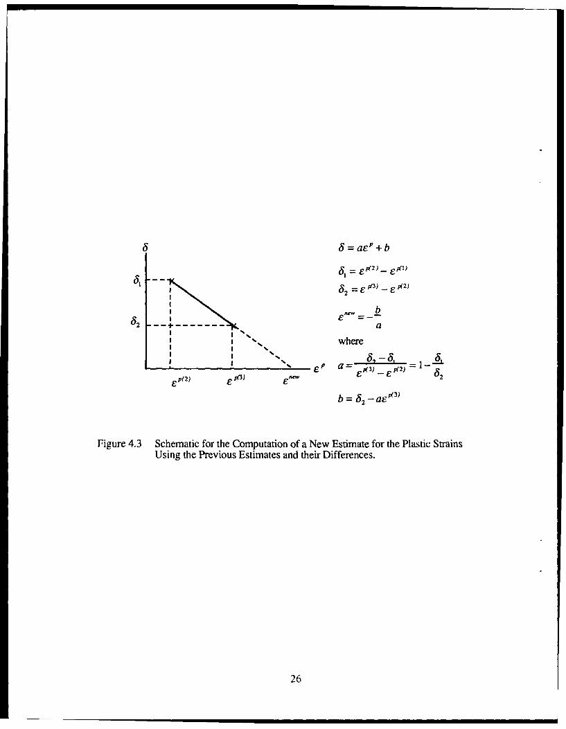
4.2 Faster Convergence Scheme

To reduce the number of iterations, a faster convergence scheme was adopted [24].In this method the three previous plastic strain increment estimates and their differences aresaved and extrapolated to a plastic strain increment that would result in a difference of zero.In Fig. 4.3, the slope of the line is calculated and the new strain is obtained as -b/a, which isthe y-intercept of the plastic strain vs. the difference graph.

25

S6 5 =ae

a +b4 5 , -", E p 2 ) _ E P M l

62 a

iwhere

" -, 6E Pa3) p(3) Ep_ ) 2

b =62 -ae p3)

Figure 4.3 Schematic for the Computation of a New Estimate for the Plastic StrainsUsing the Previous Estimates and their Differences.

26

CHAPTER 5

PROGRAM

5.1 General Description

FIDEP (Finite-Difference Code for Elastic-Plastic Analysis) is a user-friendly

computer program designed to solve the problem of concentric cylinders subjected to

thermal and mechanical loading. 1iie program is simple in structure and scope since it was

intended to be used as a practical research tool for the determination of stress concentrations

in the matrix around the fiber in unidirectional continuous fiber reinforced metal matrix

composites. The features of the program include:

"• generalized plane strain and axisymmetric geometry,

"• small displacements,

"• isotropic and incompressible fiber and matrix,

"* elastic fiber and time-independent bilinear elastic-plastic matrix

(including perfectly plastic matrix),

"• perfect bonding between the fiber and the matrix,

"• uniform temperature change throughout the composite.

More advanced features such as time-dependent material behavior, multiple

concentric cylinders are absent from the current version of the program since only speedy

prediction of the time-independent nonlinear behavior of a two-phase unidirectional

composite was required at the time.

Operation of FIDEP program is straightforward, requiring the modification of a

loading history file and a material properties data file. All input data are in free format and

some descriptive titles are allowed. The following sections describe the operation of the

program.

5.2 Program Operation

The execution of the program consists of changing two input files and executing the code.

The input files are the loading history file, FDLOAD.DAT, and temperature-dependent

constituent property data file, FDMAT.DAT. Running the code creates four output files:

27

FDOUTS, FDOUTE, FDUSP, FDSUM. The first two files consist of the stress and strainhistory, respectively, of the matrix at the interface. The output file FDUSP consists of thestress-strain distribution that exists in the composite at the end of the imposed loadinghistory. The output file FDSUM consists of a summary of the fiber and matrix stresscs atthe interface at the end of each half-cycle. In the following sections the input and output fileformats are explained in detail.

5.2.1 Input

The input consists of two files: loading file and material properties file. The loadingfile data specifies the number of steps, temperature, and applied mechanical stresses and thesecond file specifies the temperature dependent mechanical properties for the constituents.

The loading file, FDLOAD, format is listed in Table 5.1. An example loadinghistory data file for cyclic loading at room temperature after cooldown from processing is

shown in Fig. 5.1.

The material property data specifies the following properties for the matrix and thefiber: elastic modulus, coefficient of thermal expansion, Poisson's ratio, yield stress andplastic modulus for each temperature. The material data file, FDMAT, format is listed inTable 5.2. An example material data file for SCS-6 fiber and Ti-24A1-1lNb matrix material

is shown in Fig. 5.2.

5.2.2 Output

There are four output files: FDOUTS.DAT, FDOUTE.DAT, FDUSP.DAT andFDSUM.DAT. The first two files contain stresses and strains, respectively, in the matrix atthe fiber/matrix interface at each step increment. FDUSP.DAT contains the stresses andstrains along the radius for the final loading step. FDSUM.DAT contains a summary ofthe stresses and strains at the interface in the fiber and the matrix at the end points of eachcycle. The runtime is printed on the screen at the completion of the program. The outputformats are described in the following paragraphs.

FDOUTS.DAT echos the inputs from the loading and material data files at the beginning ofthe file. Following the input, the stresses and the mechanical strain in the matrix computedat the fiber/matrix interface are printed in the following order: computational step, and

28

Cooldown and Mechanical Cycling at Room TemperatureComment line 2Comment line 3Comment line 43

0 30 60 90 120 0 0 0 01010 25 25 25 25 0 0 0 00 0 350 35 350 0 0 0 0

Figure 5.1 Example Loading History Input File, FDLOAD.DAT.

TI-24-11 Matrix and SCS-6 Fiber PropertiesComment line 2211TEMP E(GPa) CTE(1E-6/C) MU SY(MPa) EP(GPa)20 413 4.72 0.3 1.E6 0.101 413 4.81 0.3 1.E6 0.203 413 4.96 0.3 1.E6 0.299 413 5.09 0.3 1.E6 0.400 413 5.23 0.3 1.E6 0.500 413 5.36 0.3 1.E6 0.598 413 5.44 0.3 1.E6 0.702 413 5.51 0.3 1.E6 0.800 413 5.66 0.3 1.E6 0.900 413 5.73 0.3 1.E6 0.1010 413 5.75 0.3 1.E6 0.8TEMP E(GPa) CTE(1E-6/C) MU SY(MPa) EP(GPa)20 84.10 11.33 0.3 950.0 0.00315. 88.40 11.88 0.3 410.0 3.29482.2 68.26 12.22 0.3 333.3 3.71649.0 48.09 12.73 0.3 256.5 4.12704.4 42.08 12.95 0.3 214.1 3.89760.0 36.07 13.22 0.3 171.8 3.67885.0 23.66 13.93 0.3 112.8 3.911010.0 11.25 14.97 0.3 53.8 4.15Reference Temperature1010Vf b

0.35 1.0

Figure 5.2 Example Material Properties Input File, FDMAT.DAT.

29

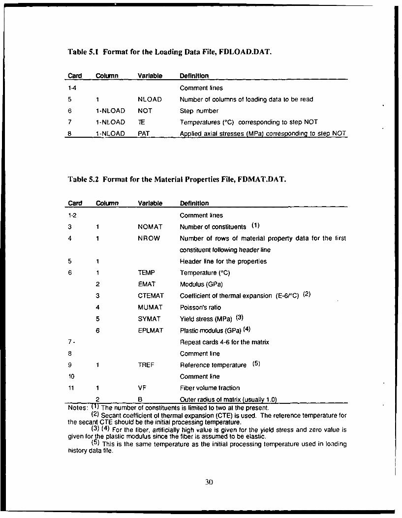
Table 5.1 Format for the Loading Data File, FDLOAD.DAT.

Card Column Variable Definition

1-4 Comment lines

5 1 NLOAD Number of columns of loading data to be read

6 1-NLOAD NOT Step number

7 1-NLOAD IE Temperatures (0C) corresponding to step NOT

8 1-NLOAD PAT Applied axial stresses (MPa) corresponding to step NOT

Table 5.2 Format for the Material Properties File, FDMAT.DAT.

Card Column Variable Definition

1-2 Comment lines

3 1 NOMAT Number of constituents (1)

4 1 NROW Number of rows of material property data for the first

constituent following header line

5 1 Header line for the properties

6 1 TEMP Temperature (0C)

2 EMAT Modulus (GPa)

3 CTEMAT Coefficient of thermal expansion (E-6/°C) (2)

4 MUMAT Poisson's ratio

5 SYMAT Yield stress (MPa) (3)

6 EPLMAT Plastic modulus (GPa) (4)

7- Repeat cards 4-6 for the matrix

8 Comment line

9 1 TREF Reference temperature (5)

10 Comment line

11 1 VF Fiber volume fraction

2 B Outer radius of matrix (usually 1.0)Notes: (1) The number of constituents is limited to two at the present.

(2) Secant coefficient of thermal expansion (CTE) is used. The reference temperature forthe secant CTE should be the initial processing temperature.

(3) (4) For the fiber, artificially high value is given for the yield stress and zero value isgiven for the plastic modulus since the fiber is assumed to be elastic.

(5) This is the same temperature as the initial processing temperature used in loadinghistory data file.

30

corresponding temperature, applied axial stress, effective stress, radial stress, hoop stress,

axial stress, original yield surface, and axial strain. The column titles are shown below.

Step Temp (Yapp Geff Or 00 Yz Y. S. Ez

The stresses are given in units of MPa, temperature in 'C, and the strain in mm/mm. The

effective stress is defined by:

,fff =---l/ 2[(a,- 6 )2 +a(a, -_ ') 2 + (o, -_ go)2]

which is equivalent to Eqn. 20.

FDOUTE.DAT consists of the strains in the matrix at the fiber/matrix interface in the

following order: computational step, and corresponding temperature, applied axial load,

radial plastic strain, hoop plastic strain, axial plastic strain, radial mechanical strain, hoop

mechanical strain, axial mechanical strain and thermal strain. The column titles are shown

below:

Step Temp Sapp -r £o Ez F-m-e f• Ezne w Cth

FDUSP.DAT consists of the stresses and plastic strains across the cross section of the

composite at the end of loading history in the following order: radius, effective stress, radial

stress, hoop stress, axial stress, radial plastic strain, hoop plastic strain and axial plastic

strain. The column titles are shown below:

Radius cSeff Or Go Uz Erp COp &zp

FDSUM.DAT consists of a summary of the stresses and strains at the interface in the fiber

and matrix at the end points of each loading/unloading cycle in the following order: step

number corresponding to steps in the loading file, FDLOAD, temperature, applied stress,

axial fiber stress, axial matrix stress, effective matrix stress, effective matrix strain and axial

mechanical strain in the matrix. The column titles are shown below:

Step Temp Gapp Ozf (yzm Qyefm eeftm E 22lenl

31

5.2.3 Program

The program FIDEP is listed in Appendix A. The program uses a default value of 50

divisions in the cylinders for applying the finite difference method. These finite difference

equations result in a linear system of 100 equations in 100 unknowns represented by the

variable NRA in the program. If a better accuracy is desired NRA can be changed to 200 in

the subroutine SOLVE.

5.2.4 Execution of FIDEP on a VAX/VMS Machine

The program FIDEP can be run interactively or in a batch mode on a VAX-VMS machine

and requires IMSL library of subroutines [271. Before execution, the program is compiled

and linked on a VAX/VMS machine as follows:

"> FOR FIDEP

"> LINK FIDEP+IMSL/LIB

To run FIDEP in real time type

> RUN FIDEP

To run FIDEP on a batch mode a command file has to be created. In this command file the

input and output files can be renamed. An example command file is shown in Fig. 5.3.

This command file is then submitted to the batch using the command

> SUBMIT/NOPRINT filename

After the job has been completed a log file will appear in the main directory.

32

$ SET VERIFY$ ASSIGN/USERYMODE [COKERDU.FIDEP]FDMAT.DAT FOMAT$ ASSIGN/USER-MODE [COKERDU. FIDEP] FDLQAD.DAT FOLOAD$ ASSIGN/USERYMODE [COKERDU.FIDEP]FDOUTS.DAT FDOUTS$ ASSIGN/USER-MODE [COKERDU.FIDEP]FDOUTE.DAT FDOUTE$ ASSIGN/USER-MODE [COKERDU.FIDEP]FDUSP.DAT FDUSP

$ ASSIGN/USER-MODE [COKERDU.FIDEP]FDSUM.DAT FDSUM$ RUN [COKERDU.FIDEP]FIDEP3B

Figure 5.3 Example Command File for Running Batch Jobs on a VAX/VMS Machine.

33

CHAPTER 6DEMONSTRATION PROBLEMS

Several problems are solved using FIDEP code to illustrate the capability forcomputing micromechanical stresses and to compare with solutions obtained by other

methods. The first case is the comparison of FIDEP solution to the closed form solution

for an elastic problem. The second case is the comparison of FIDEP results with finite

element analysis results for thermal cool-down and thermal cyclic loading. The third case isan application problem in which the stresses and strains are predicted in a unidirectional

composite subjected to in-phase and out-of-phase thermomechanical fatigue behavior and

the strains are compared with experimental measurements.

6.1 Material Properties

In these computations two-material concentric cylinder model consisting of SCS-6

silicon carbide fiber and Ti-24AI-l lNb matrix is used. The mechanical properties for SCS-6 and Ti-24A1- 11 Nb are shown in Table 6.1 as a function of temperature. The SCS-6 fiber

is isotropic and elastic with only the coefficient of thermal expansion varying with

temperature. An adequate representation of the Ti-24AI-1 1Nb matrix was attained using abilinear elastic-plastic model with temperature dependent elastic and plastic moduli, yield

stress and coefficient of thermal expansion.

6.2 Comparison with an Elastic Solution

An elastic closed form solution for two concentric cylinders and generalized

axisymmetric condition is presented in Appendix 2 [28]. The stresses at the cross-section

obtained by FIDEP and by the closed form solution for AT=-100'C is shown in Fig. 6.1.In this analysis temperature independent elastic properties were used with the followingproperties: Ef = 414 GPa, vf = 0.22, af = 4.7E-6 /1C, Em = 90 GPa, Vm = 0.30, am = 10.7E-

6 /°C, where f denotes the fiber and m denotes the matrix. The fiber volume fraction was

35%. The stresses obtained by the two method are in excellent agreement as shown in Fig.

6.1.

Stresses at the cross-section using the elastic-plastic and the elastic solution is

compared in Fig. 6.2 using the mechanical properties from Table 6.1. The temperature

34

Table 6.1 Mechanical Properties for SCS-6 Fiber and Ti-24AI-11Nb Matrix.

SCS-6 Fiber Propertiesv = 0.22

E = 414 GPa

Temperature a * (10-6/OC)(°C)

20 4.7093 4.81204 4.97316 5.12427 5.26538 5.38649 5.50760 5.60871 5.70982 5.781010 5.80

Ti-24AI-1 1 Nb Matrix Propertiesv = 0.22

Temperature a * (10-6/CC) Elastic Yield Stress Plastic(OC) Modulus (MPa) Modulus

(GPa) (GPa)

20 12.33 94 604 1.393 12.47 92 560 0.9204 12.78 91 498 0.7316 13.21 89 447 0.7427 13.75 79 421 0.4538 14.42 70 381 0.1649 15.20 50 357 0760 16.10 25 252 2.3871 17.11 18 138 2.6982 18.25 16 38 1.21010 18.55 15 30 1.0

a a is secant coefficient of thermal expansion with a reference temperature of 1010 0 C.

35

60

40FID EP .o Stress

20 Analytical Hoop Stress

0

2 -20

-40 "

'.IBR .MATRIX-60 FIBER

-80 - Axial Stress

-100 1 I I I

0 0.2 0.4 0.6 0.8

Radial Distance from the Fiber Center

Figure 6.1 Variation of Elastic Stresses with Radius Obtained by Elastic Closed-Form Solutionand FIDEP for AT = -100°C.

36

800Axial Stress

......... Elastic-Plastic400 ' .. ...... --

Elastic

Hoop Stress

0~

-40 Radial Stress S-400~

-Fiber Matrix

-800'_

..... :• . " . • } . :................. . ....:::i:: . : ... "....i

"Axial Stress-1200 1 _ 1."___:._J•______

0.0 0.2 0.4 0.6 0.8 1.0

Nondimensional Radius (r/b)

Figure 6.2 Variation of the Stresses Across the Cross-Section of the CCM After Cool-Downfrom Processing Temperature of 1010°C for Elastic and Elastic-Plastic Matrix.

37

dependent elastic solution was obtained from FIDEP by making the yield stress artificially

high (L.E6 MPa) for the matrix. The loading input file and a schematic of the loading

history is shown in Fig. 6.3. The yield surface is first reached at the interface and the

matrix near the interface becomes plastic, As the thermal loading increase the plastic zone

spreads outwards to the rest of the matrix and a redistribution of the stresses occur. In the

elastic region, the radial and hoop -resses -hange proportional to 1/"2 and the axial stress

remain uniform. Inside the plastic zone, the radial and hoop stresses remain almost uniform

and the axial stress decreases when the effective stress cannot extend beyond the yield

stress. The remaining load is redistributed to the fiber and the elastic region of the matrix.

6.3 Comparison with Finite Element Method

Two examples are presented and the results from FIDEP are compared with finite

element method (FEM) results obtained from nonlinear finite element code MAGNA [291.

The temperature dependent plasticity subroutines were implemented in MAGNA by J. L,

Kroupa [30]. The geometry and the boundary conditions for the finite element model of an

?xisymmetric concentric cylinder geometry under generalized plane strain condition are

shown in Fig. 6.4 [30]. Contact elements were used to model the fiber-matrix interface,

which allowed the separation of the fiber and matrix when the matrix stresses at the interface

became positive. Isotropic hardening model with a bilinear elastic-plastic stress-strain curve

was used to model the matrix. The fiber was elastic and the volume fraction was 35%. The

material properties listed in Table 6.1 were used for the analysis.

6.3.1 Cool-Down from Processing Temperature

The first comparison problem with FEM was the thermal cool-down associated with

processing the material. The loading input file and a schematic of the loading history is

shown in Figure 6.3. The fiber and matrix are assumed to have zero stresses and strains at

the initial consolidation temperature of 1010°C. As the material cools down, the modulus

changes with temperature and the difference in coefficient of thermal expansion between the

fiber and matrix leads to thermal stresses in the fiber and matrix. The material properties

are those shown in Table 6.1. The output from the program is presented in Appendix C.

The files FDOUTS.DAT and FDUSP.DAT were used in Figs. 6.5-6.8 discussed below.

The three-dimensional stresses computed during the cool-down process are

illustrated in Fig. 6.5. The computed stresses, shown as the dashed lines with symbols in

38

Loading File 1Cool-Down to Room TemperatureFrom a Processing Temperature of 1010°CFor SCS-6/Ti-24AI- 11Nb Unidirectional Composite20 301010 200 0

(a)

Temperature (°C)

1010

0 30 60 90 120Computational Steps

(b)

Figure 6.3 a) Loading Input File, and b) Schematic of the Temperature History for aThermal Cool-Down Simulation of SCS-6/Ti-24A1- 11 Nb UnidirectionalComposite.

39

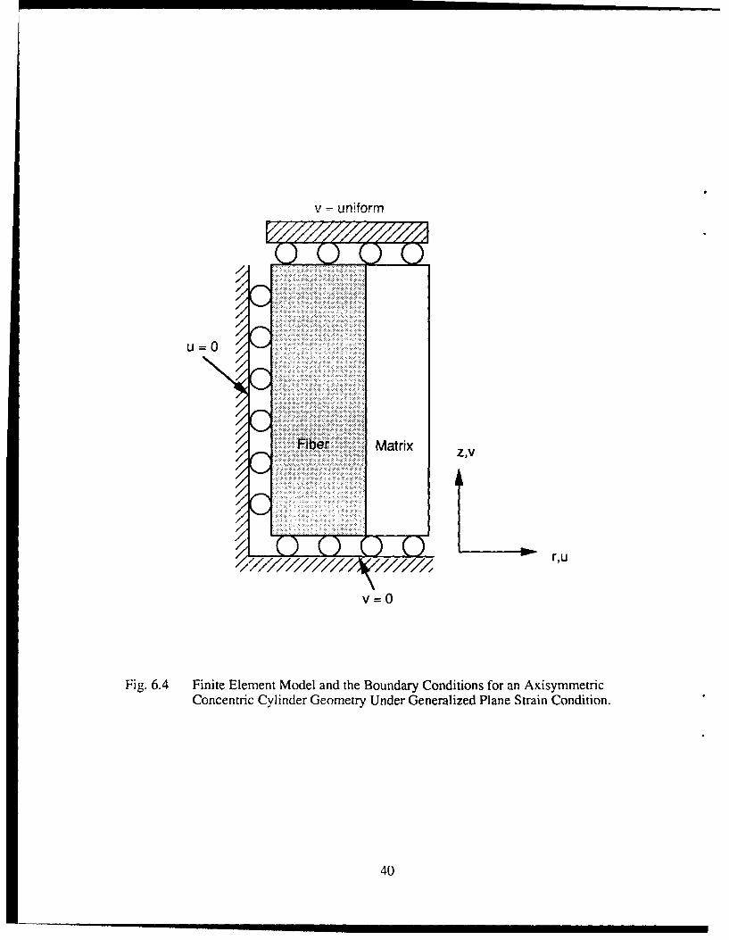
v =uniform

Fiber Matrix

v 0

Fig. 6.4 Finite Element Model and the Boundary Conditions for an AxisymmetricConcentric Cylinder Geometry Under Generalized Plane Strain Condition.

40

800 1 1 1 1 1

-..... Finite Element Method600 - •FIDEP

600-

400-40 -. Hoo p On' Oiinal -i ••CU"- Yield Surface

0-220 Axial •

-200

Radial

-400- 1 1 1 1 1

0 200 400 600 800 1000 1200Temperature (0C)

Figure 6.5. Finite Element and FIDEP Predictions for the Stresses at the Interface inTi-24AI-1 1Nb Matrix After Cool-Down from Processing Temperature of1010 0C.

41

0 .0 0 8 . . ., '' , ' , 'Effective Finite Element Method

0.006 "-+. _ _ FIDEP

S0.004 Hoop -

E 0.002C:

00

S-0.002

-0.004 Radial

-0.006

-0.008 , , , *,, , ,, . , * . .0 200 400 600 800 1000 1200

Temperature (0C)Figure 6.6 Finite Element and FIDEP Predictions of the Plastic Strains in Ti-24AI-I 1Nb

Matrix at the Fiber-Matrix Interface After Cool-Down from ProcessingTemperature of 1010°C.

42

800

- - - Effective Stress400

400 ... ---Radial Stress

- - Hoop Stresso-e-- Axial Stress

0*

, -400Plastic

Fiber Zone-800

Fiber/Matrix Interface

-1200 - _j0.0 0.2 0.4 0.6 0.8 1.0

Nondimensional Radius (r/b)

Figure 6.7 Variation of the Stresses Across the Cross-Section of the CCM AfterCool-Down from Processing Temperature of 1010'C.

43

0.008

0.006 - .o- Radial Pl. Strain-n-Hoop PI Strain

S0.004 --- -Axial P1. Strain Matrix

E 0.002E

0

-0.002 0

-0.004 "Fiber

-0.006-Plastic

SZone-0.008,

0.00 0.20 0.40 0.60 0.80 1.00NondImensional Radius (r/b)

Figure 6.8 Variation of the Plastic Strains Across the Cross-Section of the CCMAfter Cool-Down from Processing Temperature of 1010°C.

44

the plot, are compared with results for the same problem solved by FEM represented by the

solid lines. The agreement with the finite element results is excellent. The computations

show that the matrix material reaches the yield surface at approximately 600'C and remains

in contact with the yield surface for all lower temperatures. The axial and hoop stresses are

tension and the radial stress is compressive at room temperature and of equal magnitude.

The plastic strains in the matrix at the fiber-matrix interface as a function oftemperature are shown in Fig. 6.6. It can be seen here, as in Fi,. 6.5, that the matrix

deforms elastically until 600'C where the matrix stresses reach yield surface and start

deforming plastically after which measurable plastic strains develop in the three principal

directions. These results are compared with FEM computations and provide excellent

agreement as shown in the figure.

Figures 6.7-6.8 display the stresses and the plastic strains at room temperature

across the cross-section of the composite, respectively. The shaded areas denote the regionsof plastic deformation. Plasticity initiates at the interface and propagates across the matrixwith increased mechanical stress on the matrix. In this particular case, the plastic

deformation has stopped at r/b=0.91 and the rest of the matrix has remained elastic. If atensile mechanical load is superimposed at room temperature this will further propagate theplastic region until all the matrix yields.

6.3.2 Cyclic Thermal Loading

In this example the SCS-6/Ti-24A1- 11 Nb composite is thermally cycled between

processing temperature and room temperatcure as shown in Fig. 6.9. The effective stress

and the radial stress as a function of temperature are plotted and compared with results fromFEM in Fig. 6. 10. FIDEP results are in excellent agreement with finite element resultsprior to attaining a temperature of 850'C at the end of the first cycle. The two methods

digress after 850'C because of the changing of the compressive matrix radial stresses at theinterface to tensile at this temperature (Fig. 6. 10). In the case of the tensile radial stress thefinite element model asssumes debonding of the matrix from the fiber to occur whereas the

present model assumes perfect bonding. Thus, the two methods predict different but similar

states after debonding takes place.

45

Loading File 1Cyclic Thermal LoadingBetween Room Temperature and Processing TemperatureTemperature: 20 C to 1010 C40 30 90 1201010 20 1010 200 0 0 0

(a)

Temperature (°C)

1010

200 30 90 120

Computational Steps

(b)

Figure 6.9 a) Loading Input File, and b) Schematic of the Temperature History forThermal Cyclic Loading Simulation of SCS-6/Ii-24A1- II NbUnidirectional Composite.

46

800FIDEP --------- FEM

600Original

Yield Surface

400 Effective

200+"Stress Stre+s__2 5- ++/

"20200 600 +(,/) • •+++

37+ 4Co•

-200-

Radial Stress

-400 1 10 200 400 600 800 1000 1200

Temperature (°C)

Figure 6.10 FIDEP and FEM Predictions for the Effective and Radial Stressesin the Matrix at the Fiber-Matrix Interface for Thermal Loading Historyshown in Fig. 6.9.

47

6.4 Thermomechanical Fatigue (TMF)

The FIDEP code was used to compute stresses for simulated TMF cycles toillustrate the micromechanical stresses developed during two typical TMF tests on a SCS-

6/Ti-24AI- 11 Nb composite. The two tests are in-phase (IP) and out-of-phase (OOP) cycles

and are shown schematically in Fig. 6.11. In both tests, the first part of the cycle is thecool-down from processing temperature discussed previously. This is accomplished under

zero external load conditions. The horizontal axis in Fig. 6.11 represents an arbitrary time

scale and is shown in terms of computational steps. Step 20 represents the roomtemperature condition after cool-down. The values shown in the figure correspond to TMF

cycles which were evaluated experimentally and involve a maximum stress of 800 MPa,R=0. 1 (ratio of minimum to maximum stress) for the OOP and IP cases, and a temperature

range of 150 to 650'C.

The variation of the stresses across the cross section for an OOP cycle is illustratedin Fig. 6.12. The stresses in both fiber and matrix are shown at the minimum temperature

(maximum load) in (a) while stresses at maximum temperature (minimum load) arepresented in (b). At 1500C, Fig. 6.12(a) shows a large tensile axial stress in the fiber and

tensile axial stresses in the matrix. The fiber stresses are essentially independent of radial

coordinate, but the matrix stresses vary significantly with radius because of the complexthree-dimensional stress state which arises in the concentric cylinder configuration. Matrix

axial stresses are maxim'am at the outer radius and minimum at the fiber-matrix interface.Hoop stresses, on the other hand, are minimum at the outer radius of the cylinder but do notvary as much as the axial component. The matrix radial stress is negative at the fiber-matrix

interface and goes to zero at the outer radius because of the imposed stress-free boundarycondition. The stresses developed are the net result of the thermal stresses developed at a

low temperature, the axial component of which is compression in the fiber and tension in thematrix, and the applied mechanical stresses which are tension in both fiber and matrix in the

axial direction.

At elevated temperature in an OOP TMF cycle, the stress state is generally small as

shown in Fig. 6.12(b). Under this condition, the thermal stresses are small because at hightemperature the stresses are relaxed while the mechanical stresses are small because this is

the condition of minimum load.

48

Loading File 1Cool-Down and In-Phase TMF LoadingLoad: 80 MPa to 800 MPaTemperature: 150 C to 650 C70 30 60 90 120 150 1801010 20 650 150 650 150 6500 0 800 80 800 80 800

Loading File 2Cool-Down and Out-of-Phase TMF LoadingLoad: 80 MPa to 800 MPaTemperature: 150 C to 650 C70 30 60 90 120 150 1801010 20 650 150 650 150 6500 0 80 800 80 800 80

(a)

S1000 1 1 1080. 800 -In-Phase

o 600. 400-

-o 200-

0~ CpOut-of-PhaseQ-1000 C3

0 30 6 0 90 12'0 150 80 1 .'_0Computational Step

(b)

Figure 6.11 a) Loading Input Files, and b) Schematic of the Temperature and StressHistory for Typical In-Phase and Our-of-Phase TMF Cycles.

49

1200Fiber Matrix

1000

800 - Radial Stress600 Hoop Stress

-e-- Axial Stress

400

S 200 Fiber/MatrixWm Interface

0-

-200

0 0.2 0.4 0.6 0.8

Radius (r/b)

Figure 6.12a Variation of Predicted Stresses with Radius for an Out-of-Phase TMFCycle at 150'C.

50

1200

1000 Fiber Matrix

800 Radial Stress

-600 -- Hoop Stress-e-- Axial Stress Fiber/Matrix

Interface400

co 200

0

-200

-400 ' " ' ' ' ' ' ' ' '

0 0.2 0.4 0.6 0.8Radius (r/b)

(b)

Figure 6.12b Variation of Predicted Stresses with Radius for an Out-of-Phase TMF Cycleat 650 0C.

51

The axial stresses in the matrix at the fiber-matrix interface are shown in Fig. 6.13.The steps on the horizontal axis correspond to those of the TMF spectrum schematic in Fig.

6.1 lb. As noted in the discussion of the previous figure, the OOP cycle has tensile thermalstresses as well as tensile mechanical stresses at minimum temperature which corresponds

to maximum load. This results in a large stress range in the matrix from approximately 450

MPa at minimum temperature (step 60) to approximately -50 MPa at maximum temperature(step 80). The IP cycle, on the other hand, has a much smaller stress range in the matrix

material. At minimum temperature (step 60), there is a thermal residual stress but little

contribution from applied (minimum) load. The net stress is approximately 275 MPa.When maximum temperature is reached (step 80), the thermal stress decreases and the

mechanical stress increases. The net result is a stress decrease to approximately 200 MPa.In summary, the axial stress range in the matrix is large in an OOP cycle and small in an IP

cycle.

In a similar fashion, the axial stress peaks in the fiber are compared for an IP and

OOP TMF cycle in Fig. 6.14. In the fiber, the thermal stresses at low temperature arecompressive because of the low value of a compared to that in the matrix. For an IP cycle,

therefore, the axial stresses range from compressive, due to residual thermal stress at low

temperature (step 60), to tension due to the applied maximum load at high temperature (step

80). In the OOP cycle, the compressive residual stress at low temperature is offset by the

larger mechanical stress due to maximum load, resulting in a net tensile stress of

approximately 1000 MPa at minimum temperature (step 60). Decreasing the load whileincreasing the temperature reduces the mechanical stress but also relaxes the compressive

residual stress. Since the mechanical stress range exceeds the thermal stress range for this

set of conditions, the net effect is a reduction in stress to approximately 200 MPa atmaximum temperature (step 80). Thus, an in-phase cycle produces a larger stress range and

higher maximum stress in the fiber than an out-of-phase cycle for the conditions evaluated

here. This is in contrast to the stress range in the matrix which is maximum in the OOP

cycle and smaller in the IP cycle.

The radial and hoop stresses in the matrix at the fiber-matrix interface are plotted inFig. 6.15. Since the applied load is in the axial direction, its contribution to hoop and radial

stresses is minimal and arises solely due to Poisson's ratio and 3-D plasticity effects. Thus,

the stresses are mostly due to the thermal cycling, and the IP and OOP cycles produce a

similar stress state. At minimum temperature (step 60), the hoop stresses in the matrix are

52

700

0 Out-of-Phase600 . In-Phase

500 -

D 400 -

300 -,,-I I

75 200-

100

0

-100 I i i i i I I0 20 40 60 80 100 120 140 160 180 200

Computation Step

Figure 6.13 Axial Stress Predictions in the Ti-24Al-11Nb Matrix at the Fiber-MatrixInterface for In-Phase and Out-of-Phase TMF Cyclic Loading.

53

2000-- Out-of-Phase

1500.In-Phase1500

I'

SI I

1000I I

S500 -

U)%

< 0

-1000 I I

0 20 40 60 80 100 120

Computation Step

Figure 6.14 Axial Stress Peaks Predicted in the SCS-6 Fiber for In-Phase and Out-of-PhaseTMF Cyclic Loading.

54

400 I ,Out-of-Phase

300 In-Phase Hoop StressI'#I %

I IIk200

S100 ' '

U) %.

a, #

v ~%#if.1

-100 %% %

-200 %

Radial Stress-300 I I I I

0 20 40 60 80 100 120

Computation Step

Figure 6.15 Radial and Hoop Stress Predictions in Ti-24AI-11 Nb Matrix at the Fiber-MatrixInterface for In-Phase and Out-of-Phase TMF Cyclic Loading.

55

tensile whereas the radial stresses are compressive. At the maximum temperature (step 80),both components relax to nearly zero.

56

REFERENCES

[ 1 Foye, R. L., "Theoretical Post-Yielding Behavior of Composite Laminates, Part I- Inelastic Micromechanics", Journal of Composites Materials, Vol. 7, No. pp.178-193, April 1973.

[2] Lin, T. H., Salinas, D., and Ito, Y. M., "Elastic-Plastic Analysis of UnidirectionalComposites", Journal of Composite Materials, Vol. 6, No. pp. 48-60, 1972.

[31 Adams, D. F., "Inelastic Analysis of a Unidirectional Composite Subjected toTransverse Normal Loading", Journal of Composite Materials, Vol. 4, No. pp.310-328, 1970.

[41 Foye, R. L., "Inelastic Micromechanics of Curing Stresses in Composites",Inelastic Behavior of Composite Materials, 1975 ASME Winter AnnualMeeting, C. T. Herakovich, Eds., American Society of Mechanical Engineering,Houston, Texas, pp. 1975.

[51 Kolkailah, F. A. and McPhate, A. J., "Bodner-Partom Constitutive Model andNonlinear Finite Element Analysis", Journal of Engineering Materials andTechnology, Vol. 112, No. pp. 287-291, July 1990.

161 Sherwood, J. A. and Boyle, M. J., "Investigation of the ThermomechanicalResponse of a Titanium-Aluminide/Silicon-Carbide Composite using a UnifiedState Variable Model and the Finite Element Method", Microcracking-InducedDamage in Composites, AMD-Vol. 111/MD-Vol. 22, , Eds., The AmericanSociety of Mechanical Engineers, pp. 151-161, 1990.

[71 Dvorak, G. J. and Bahei-E1-Din, Y. A., "Plasticity Analysis of FibrousComposites", Journal of Applied Mechanics, Vol. 49, No. pp. 327-335, June1982.

[81 Bahei-EI-Din, Y. A., Plastic Analysis of Metal-Matrix Composite Laminates,Ph. D. Dissertation, Duke University, 1979.

19) Mirdamadi, M., Johnson, W. S., Bahei-EI-Din, Y. A., and Castelli, M. G.,Analysis of Thermomechanical Fatigue of Unidirectional Titanium MetalMatrix Composites, NASA Technical Memorandum 104105, July 1991.

1101 Aboudi, J., "Damage in Composites - Modeling of Imperfect Bonding",Composites Science and Technology, Vol. No. 28, pp. 103-128, 1987.

11I Hopkins, D. A. and Chamis, C. C., "A Unique Set of Micromechanics Equationsfor High-Temperature Metal Matrix Composites", Testing Technology of MetalMatrix Composites, ASTM STP 964, P. R. DiGiovanni and N. R. Adsit, Eds.,American Society for Testing and Materials, Philadelphia, pp. 159-176, 1988.

1121 Sun, C. T., Chen, J. L., Shah, G. T., and Koop, W. E., "MechanicalCharacterization of SCS-6/Ti-6-4 Metal Matrix Composite", Journal ofComposite Materials, Vol. 24, No. pp. 1029-1059, October 1990.

57

[131 Chamis, C. C. and Hopkins, D. A., "Thermoviscoplastic Nonlinear ConsitutiveRelationships for Structural Analysis of High-Temperature Metal MatrixComposites", Testing Technology of Metal Matrix Composites, ASTM STP964, P. R. DiGiovanni and N. R. Adsit, Eds., American Society for Testing andMaterials, Philadelphia, pp. 177-196, 1988.

[14] Chamis, C. C., Murthy, P. L. N., and Hopkins, D. A., "Computational Simulationof High-Temperature Metal Matrix Composites Cyclic Behavior", Thermal andMechanical Behavior of Metal Matrix and Ceramic Matrix Composites,ASTM STP 1080, J. M. Kennedy, H. H. Moeller, andW. S. Johnson, Eds.,American Society for Testing and Materials, Philadelphia. pp. 56-69, 1990.

[151 Bigelow, C. A., Johnson, W. S., and Naik, R. A., "A Comparison of VariousMicromechanics Models for Metal Matrix Composites", Mechanics ofComposite Materials and Structures, J. N. Reddy and J. L. Telpy, Eds., TheAmerican Society of Mechanical Engineers, Philadelphia, pp. 21-31, 1989.

[161 Mikata, Y. and Taya, M., "Stress Field in a Coated Continuous Fiber CompositeSubjected to Thermo-Mechanical Loadings", Journal of Composite Materials,Vol. 19, No. pp. 554-578, November 1985.

[17] Vedula, M., Pangborn, R. N., and Queeney, R. A., "Modification of ResidualThermal Stress in a Metal-Matrix Composite with the use of a Tailored InterfacialRegion", Composites, Vol. 19, No. 2, pp. 133-137, March 1988.

[18] Pagano, N. J. and Tandon, G. P., "Elastic Response of Multi-Directional Coated-Fiber Composites", Composites Science and Technology, Vol. 31, No. pp. 273-293, 1988.

[19] Ebert, L. J., Fedor, R. J., Hamilton, C. H., Hecker, S. S., and Wright, P. K.,Analytical Approach to Composite Behavior, Technical Report AFML-TR-69-129, June 1969.

[20] Hecker, S. S., Hamilton, C. H., and Ebert, L. J., "Elastoplastic Analysis ofResidual Stresses and Axial Loading in Composite Cylinders", Journal ofMaterials, JMLSA, Vol. 5, No. 4, pp. 868-900, December 1970.

[21] Gdoutos, E. E., Karalekas, D., and Daniel, I. M., "Thermal Stress Analysis of aSilicon Carbide/Aluminum Composite", Experimental Mechanics, Vol. 31, No.3, pp. 202-208, September 1991.

122] Gdoutos, E. E., Karalekas, D., and Daniel, I. M., "Micromechanical Analysis ofFilamentary Metal Matrix Composites Under Longitudinal Loading", Journal ofComposites Technology and Research, JCTRER, Vol. 13, No. 3, pp. 168-174,Fall 1991.

[231 Lee, J. W. and Allen, D. H., "An Analytical Solution for the ElastoplasticResponse of a Continuous Fiber Composite Under Uniaxial Loading", Researchin Structures, Structural Dynamics and Materials 1990, NASA ConferencePublication 3064, pp. 55-65, 1990.

1241 Timoshenko, S. P. and Goodier, J. N., Theory of Elasticity, New York,McGraw-Hill Book Company, 1987.

58

1251 Mendelson, A., Plasticity: Theory and Application, New York, MacMillan,1968.

1261 Chakrabarty, J., Theory of Plasticity, New York, McGraw-Hill Book Company,1991.

1271 IMSL FORTRAN Subroutines for Mathematical Applications, Math/LibraryVersion 1.0, IMSL, Houston, 1987.

1281 Ashbaugh, N. E., Khobaib, M., et al., Mechanical Properties for AdvancedEngine Materials, WL-TR-91-4149, Materials Directorate, Wright Laboratory,Wright-Patterson AFB, Ohio, April 1992.

1291 Brockman, R. A., "MAGNA: A Finite System for Three Dimensional NonlinearStatic and Dynamic Structural Analysis", Computers and Structures, Vol. 13,No. pp. 4'5-423, 1981.

1301 Kroupa, J. L., "Elastic-Plastic Finite Element Analysis of MMC Subjected toThermomechanical Fatigue", Titanium Aluminide Composites, WL-TR-91-4020, Wright Laboratory, Wright-Patterson AFB, Ohio, February, 1991.

59

APPENDIX ALISTING OF FIDEP SOURCE CODE

60

PROGRAM FIDEP3B

CC

C THIS PROGRAM COMPUTES ELASTIC-PLASTIC STRESSES IN AXISYMMETRIC

C CONCENTRIC CYLINDERS SUBJECTED TO THERMOMECHANICAL CYCLIC

C LOADING.

C

C INPUT FILES:

C FDMAT TEMPERATURE DEPENDENT MATERIAL DATA

C FDLOAD THERMOMECHANICAL CYCLIC LOADING PROFILE

C OUTPUT FILES:

C AT INTERFACE:

C FDOUTS STRESSES AND AXIAL STRAIN AT EACH STEP

C FDOUTE STRAINS AT EACH STEP

C FDSUM STRESSES AND STRAINS CORRESPONDING TO FDLOAD

C AT CROSS-SECTION:

C FDUSP STRESSES AND STRAINS AT THE END OF THE PROGRAM

C AT THE COMPOSITE CROSSSECTION

C

C FINAL REVISION: 13-NOVEMBER-1991

C PROGRAMMER: DEMIRKAN COKER (255-1361)

C SUPERVISOR: NOEL E. ASHBAUGHr UNIVERSITY OF DAYTON RESEARCH INSTITUTE

C

C

C DEFINITION OF THE VARIABLES USED IN THE PROGRAM

C /MAT1/

C E(201) MODULUS AT RADIUS R

C VMU(201) POISSON'S RATIO AT EACH R

C CTE(201) THERMAL EXPANSION COEFFICIENT AT EACH R

C R(201) RADIUS

C VF FIBER VOlIUMF FRACTION

C EZ EZ = EZSTAR - 2/EC*SR(INT+1)*VF*(VMU(INT)-VMU(INT+1))

C I.E. TOTAL AXIAL STRAIN = EZTOT

C /MAT2/

C EC RULE OF MIXTURES COMPOSITE MODULUS

61

C TEMP(5,20) TEMPERATURES AT WHICH PROPERTIES ARE GIVEN FOR

C CONSTITUENTS

C EMAT(5,20) MODULI AT TEMPERATURE FOR THE CONSTITUENTS

C CTEMAT(5,20) CTES AT TEMPERATURE FOR THE CONSTITUENTS

C VMUMAT(5,20) POISSON'S RATIOS AT TEMPERATURE FOR THE CONSTITUENTS

C /MAT3/

C DT(200) CURRENT TEMPERATURE MINUS REFERENCE TEMPERATURE

C T(200) CURRENT TEMPERATURE

C ET(5,200) CONSTITUENT MODULI INTERPOLATED FOR THE CURRENT

C TEMPERATURE

C VMUT(5,200) CONSTITUENT POISSON'S RATIIO .. .." ..

C CTET(5,200) CONSTITUENT CTE INTERPOLATED .. . ..

C PZ(200) APPLIED STRESS CORRESPONDING TO THE CURRENT STEP

C /MAT4/

C TINI,TFIN INITIAL AND FINAL TEMPS READ FROM THE LOADING FILE

C PINI,PFIN INITIAL AND FINAL APPLIED STRESSES READ FROM THE

C LOADING FILE

C TREF REFERENCE TEMPERATURE FOR SECANT CTE = PROCESSING

C TEMPERATURE WHERE THE STRESSES ARE ASSUMED TO BE ZERO

C /MAT5/

C SYMAT(5,20) ORIGINAL YIELD STRESS AT DEFINED TEMPERATURES

C EPLMAT(5,20) PLASTIC MODULUS FOR THE CONSTITUENTS AT DEFINED

C TEMPERATURES

C /MAT6/

C EPLT(5,200) CONSTITUENT PLASTIC MODULI INTERPOLATED FOR THE

C CURRENT TEMP

C SY(5,200) CONSTITUENT ORIGINAL YIELD INTERPOLATED FOR THE

C CURRENT TEMP

C /LIMITS/

C NTOT NUMBER OF NODES ALONG THE RADIUS MINUS 1 = NRA/2.

C NRA NUMBER OF ROWS OF MATRIX A

C INT NODE IN THE FIBER AT THE INTERFACE

C /STRAINS/

C ERTOT(201) TOTAL RADIAL STRAIN

C ETTOT(201) TOTAL HOOP STRAIN

C EZTOT(201) TOTAL AXIAL STRAIN

62

C /XX/

C ERP(201),ETP(201),EZP(201)

C OLD PLASTIC STRAINS IN THE PLSTRAIN .NE. NEW PLASTIC

C STRAINS IN SUBROUTINE SOLVE WHICH DOES NOT USE THIS

C COMMON BLOCK

C ERP2(201), ETP2(201), EZP2(201)

C PLASTIC STRAINS USED IN SUBROUTINES PLSTRAIN AND SOLVE

C /LEG/

C JAR TO READ NRA FROM SUBROUTINE SOLVE AT THE BEGINNING

C SR(Z@1) RADIAL STRESS ACROSS THE CROSSSECTION

C ST(201) HOOP STRESS ACROSS THE CROSS-SECTION

C SZ(2ol) AXIAL STRESS ACROSS THE CROSS-SECTION

C NOMAT NUMBER OF MATERIALS - FOR NOW 2

C NROW(S) NUMBER OF ROWS OF TEMPERATURE DEPENDENT DATA

C SE(201) CURRENT YIELD SURFACE - USED IN SUBROUTINE PLSTRAIN

C TE(20) TEMPERATURE READ FROM LOADING FILE

C PAT(20) APPLIED STRESS READ FROM LOADING FILE

C NOT(20) TOTAL NUMBER OF STEPS FOR EACH HALF CYCLE

C

C ****** ****** **** *************' *****

COMMON/MATO/EF,EM,CTEF,CTEM

COMMON/MATi/EC,E(201),VMU(201),CTE(201),R(201),VF,EZ

COMMON/MAT2/TEMP(5,20),EMAT(5,20),CTEMAT(5,20),VMUMAT(5,20)

COMMON/MAT3/DT(200),T(200),ET(5,200),VMUT(5,200),CTET(5,200),PZ(200)

COMMON/MAT4/TINI,TREF,TFIN,PINI,PFIN

COMMON/MAT5/SYMAT(5,20), EPLMAT(5,20)

COMMON/MAT6/EPLT(5,200), SY(5,200)

COMMON/LIMITS/NTOT, NRA, INT

COMMON/STRAINS/ERTOT(201), ETTOT(201), EZTOT(201)

COMMON/LEG/JAR

COMMON/EMECH/ETHERMAL,ERMECH,E- EMECH,EZMECHREAL ERP2(201),ETP2(201),EZPZ(201)

REAL SR(201), ST(201), SZ(201), SEFF(201), SE(201)

INTEGER NOMAT, NROW(5)

INTEGER NTIME

REAL TE(20), PAT(20), NOT(20)

6(3

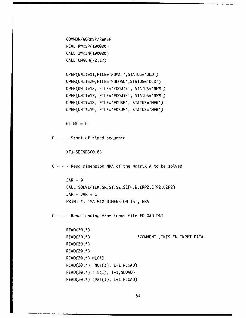
COMMON/WORKSP/RWKSP

REAL RWKSP(100000)

CALL IWKIN(100000)

CALL UMACH(-2,12)

OPEN(UNIT=11,FILE='FDNIAT' ,STATUS='OLD')

OPEN(UNIT~=20,FILE='FDLOAD' ,STATUS='OLD')

OPEN(UNIT=1Z, FILE='FDOUTS', STATUS='NEW')

OPEN(UNIT=17, FILE='FDOUTE', STATUS='NEW')

OPEN(UNIT=18, FILE='FDUSP', STATUS='NEW')

OPEN(JNIT=19, FILE~='FDSUM', STATUS='NEW')

NTIME = 0

C - - - Start of timed sequence

XT1=SECNDS(0 .0)

C - - - Read dimension NRA of the matrix A to be solved

JAR = 0

CALL SQLVE(ILK,SR, ST,SZ ,SEFF ,B,ERP2 ,ETP2 ,EZPZ)

JAR = JAR + 1

PRINT *, 'MATRIX DIMENSION IS', NRA

C - - - Read loading from input file FDLQAD.DAT

REAO(20, *)

READ(20,*) !COMMENT LINES IN INPUT DATA

READ(20,*)

READ(20, *)

READ(20,*) NLOAD

READ(20,*) (NOT(I), I=I,NLOAD)

READ(20,*) (TE(I), I=1,NLOAD)

READ(ZO,*) (PAT(I), I=1,NLOAD)

64

WRITE(12,*) 'NO OF DATA ', NLOAD

WRITE(12,*) 'STEPS', (NOT(I), I=1,NLOAD)

WRITE(12,*) 'TEMP ', (TE(I), I=1,NLOAD)

WRITE(12,*) 'STRESS ', (PAT(I), I=1,NLOAD)

TREF =TE(1)

C - - - Read temperature dependent material properties

CALL READMAT(NOMAT,NROW)

C - - - Define nodes in the concentric cylinder model

CALL GEOMETRY(VF,B,A,DR,R)

C - - - Print header lines

CALL HEADER(NTIME,TE,PAT,NOT)

CLQSE(11)

CLQSE(20)

C - - - Start cyclic loading

DO 995 ICYC = 1, NLOAD-1

NSTEPS = NOT(ICYC+1)-NOT(ICYC)

TINI = TE(ICYC)

TFIN = TE(ICYC+1)

PINI = PAT(ICYC)*l.OE6

PFIN = PAT(ICYC+1)*1.0E6

CALL LOADING(NSTEPS ,NOMAT)

DO 990 ILK=2,NSTEPS+1

NTIME = NTIME + 1

65

C - - - Define properties at each node, i. e. translate properties at

C temperature for material 1 and 2 into node properties; E,alpha,nu

C In addition, define shorthands for moduli, Ef, Em, Ec.

CALL PROPERTIES(ILK)

C - - - Calculate stresses with old plastic strains (dep-new = 0)

C i.e. assume loading increment to be elastic only

CALL SOLVE(ILK,SR,ST,SZ,SEFF,B,ERP2,ETPZ,EZP2)

C - - - Iterate to find plastic strain increments

CALL PLSTRAIN(ILK,SR,ST,SZ,SEFF,B,ERPZ,ETP2,EZPZ,SE)

C - - - Output stresses and strains

CALL OUTS(SEFF,SR,ST,SZ,ILK,NTIME,ERP2,ETP2,EZP2)

990 CONTINUE

CALL OUTSUM(INT,SZ,SR,ST,SEFF,NTIME,TFIN,PFIN)

995 CONTINUE

C - - - Output stresses and strains at the cross-section

CALL OUTUSP(SEFF,SR,ST,SZ,ERP2,ETP2,EZP2,NTOT)

C - - - Print out runtime of the code

CALL REALTIME(NRA,NTIME,XT1)

99 FORMAT(2X,I4,1X,F7.1,1X,F8.1,1X,5(F8.1,1X),E1O.3)

STOP

END

66

C ---------------------

C SUBROUTINESC - - - - - - - - - - - - - - - - - - - - - - - - - - - - - - - - - - - - - - - - - - - - - - - - - - - - - - - - - - - - - - - - - - - - -.

C - - - - - - - - - - - - - - - - - - - - - - - - - - - - - - - - - - - - - - - - - - - - - - - - - - - - - - - - - - - - - - - - - - - - -

C READ INPUT MATERIAL PROPERTIES FOR THE FIBER AND THE MATRIX

C ---------------------------------------------------------------------

SUBROUTINE READMAT(NOMAT,NROW)

COMMON/MATZ/TEMP(5,ZO),EMAT(5,20),CTEMAT(5,20),VMUMAT(5,20)

COMMON/MAT4/TINI,TREF,TFIN,PINI,PFIN

COMMON/MAT5/SYMAT(5,20), EPLMAT(5,20)

REAL TEMP,EMAT,CTEMAT,VMUMAT,TREF,TFIN,TREF2(5)

INTEGER NOMAT,NROW(5)

C - - - Read temperature dependent material data

READ(11,*)

READ(11,*)

READ(11,*)NOMAT

DO 144 I=1,NOMAT

READ(11,*) NROW(I)

READ(11,*)

DO 144 J=1,NROW(I)

READ(11,*) TEMP(I,J),EMAT(I,J),CTEMAT(I,J),VMUMAT(I,J),

+ SYMAT(I,J), EPLMAT(I,J)

WRITE(12,99)I,J,TEMP(I,J),EMAT(I,J),CTEMAT(I,J),VMUMAT(I,J),

+ SYMAT(I,J), EPLMAT(I,J)

144 CONTINUE

99 FORMAT(2(I5),2X,4(F8.2),E9.2,F8.2)

READ(11,*)

READ(11,*)TREF

RETURN

END

67

C COMPUTE RADIUS OF NODES AND INTERFACE NODE IN THE CCM

C--------------------------------------------------------------------

SUBROUTINE GEOMETRY(VF,B,A,DR,R)

COMMON/LIMITS/NTOT, NRA, INT

REAL VF, B, A, DR, R(201)

INTEGER NTOT, INT

READ(11,*)

READ(11,*,END=44) VF, B

WRITE(12,*)'VF= ', VF

GOTO 45

44 VF = 0.35

B = 1.

45 A = SQRT(VF)/B

PRINT *, 'VF, B ', VF, B

NTOT = NRA/2.0

C - - - Nodes in Fiber

R(1) = 0.02E-10

R(2) = A/2

R(3) = A - A/100.0

C - - - Nodes in Matrix

R(4) = A + A/100.0

DR = (B-A)/(NTOT-3)

DO 10 I=S,NTOT+1

R(I) = A + DR*(I-4)

10 CONTINUE

INT = 3 !A/DR + 1

DO I=1,NTOT+1

PRINT *, I, R(I)

END DO

PRINT *, ' rf, rm, A ', R(INT), R(INT+1),A

C R(INT+l) = A

RETURN

END

68

C - - - - - - - - - - - - - - - - - - - - - - - - - - - - - - -- - - -

C COMPUTE INCREMENTAL LOADING AND INTERMEDIATE PROPERTIES

C--------------------------------------------------------------------

SUBROUTINE LOADING(NSTEPS ,NOMAT)

COMMON/MAT3/DT(200) ,T(200), ET(5 , 20) ,VMUT(5 ,200) ,CTET-(5,200) ,PZ(200)

COMMON/MAT4/TINI ,TREF , FIN ,PINI ,PFIN

COMMON/MAT2/TEMP(5 ,20) ,EMAT(5 ,20), CTEMAT(5, 20) ,VMUMAT(5 ,20)

COMMON/MAT5/SYMAT(5 ,20), EPLMAT(5 ,20)

COMMON/MATh/EPLT(5 ,200), SY(5, 200)

DO 110 I=1,NSTEPS+l

DTII = (I-1.)*(TFIN-TREF)/NSTEPS/1.

DTEMP = (I-1.)*(TFIN-TINI)/NSTEPS/1.

T(I) =TINI + DTEMP

DPZ = (I-1.)*(PFIN-PINI)/NSTEPS/1.

PZ(I) = PINI + DPZ

DT(I) = T(I) - TREF

TT = T(I)

C - - - Compute the material properties at each loading temiperature

DO K=1,NOMAT

J= 1

DO WHILE(TT.GT.TEMP(K,J))

3=3+1

END DO

TFACTOR=(TT-TEMP(K,J-1))/(TEMP(K,J).TEMP(K,3-1))

CALL INTERP(I,K,J,TFACTOR,ET,EMAT)

CALL INTERP(I ,K,J ,TFACTOR,CTET,CTEMAT)

CALL INTERP(I ,K,J,TFACTOR,VMUT,VMUMAT)

CALL INTERP(I,K,J,TFACTOR,SY,SYMAT)

CALL INTERP(I,K,J ,TFACTOR,EPLT,EPLMAT)

END DO

69

11.0 CONTINUE

DO 120 K=1,NOMAT

DO 120 I=I,NSTEPS+1

SY(K,I) = SY(K,I)*1.E6

EPLT(K,I) = EPLT(K,I)*I.E9

120 CONTINUE

RETURN

END

C ---------------------------------------------------------------------

C INTERPOLATION SCHEME USED IN DETERMINING INTERMEDIATE PROPERTIES

C ----------------------------------------------------------------------

SUBROUTINE INTERP(I,K,J,TFACTOR,VALT,VALMAT)

REAL VALT(5,200), VALMAT(5,20), TFACTOR

INTEGER I, K, J

VALT(K,I)=VALMAT(K,3-1)+(VALMAT(K,J)-VALMAT(K,3-1))*TFACTOR

RETURN

END

C ---------------------------------------------------------------------

C ASSIGN PROPERTIES TO EACH NODE

C ---------------------------------------------------------------------

SUBROUTINE PROPERTIES(ILK)

COMMON/MATO/EF,EM,CTEF,CTEM

COMMON/MATI/EC,E(201),VMU(201),CTE(201),R(201),VF,EZ

COMMON/MAT3/DT(200),T(200),ET(5,200),VMUT(5,200),CTET(5,200),PZ(200)

COMMON/MAT6/EPLT(5,200), SY(5,200)

COMMON/LIMITS/NTOT, NRA, INT

EF = ET(1,ILK)*1.E9 !414E9

EM = ET(2,ILK)*1.E9 !113.7E9

70

CTEF = CTET(1,ILK)*1.0E-6

CTEM = CTET(2,ILK)*1.0E-6

DO 21 I=1,INT

E(I) = ET(1,ILK)*1.E9 !414.E9

VMU(I) = VMUT(1,ILK) !0.3

CTE(I) =CTET(1,ILK)*1.E-6 !4.7E-6

21 CONTINUE

DO 22 I=INT+1,NTOT+1

E(I) = ET(2,ILK)*l.E9 !113.7E9

VMU(I) = VMUT(2,ILK) !0.22

CTE(I) = CTET(2,ILK)*1.E-6 !9.44E-6

22 CONTINUE

EC = EF*VF + EM*(1=VF)

RETURN

END

71

C -- - - - - - - - - - - - - - - - - - - - - - - - - - - - - - - - - -

C COMPUfE STRESSES GIVEN A PLASTIC STRAIN INCREMENT

C--------------------------------------------------------------------

SUBROUTINE SOLVE(ILK,SR,ST,SZ ,SEFF ,B,ERP,ETP,EZP)

PARAMETER(NRA=100, LDA~=NRA, IPATH=1)

COMMON/LIMITS/NTOT,NNRA, TNT

COMMON/MATO/EF ,EM, (TEF ,CTEM

COMMON/MATi/EC ,E(201) ,VMU(201) ,CTE(201) ,R(201) ,VF ,EZ

COMMON/MAT3/DT(200) ,T(200) ,ET(5,200) ,VMUT(5,200) ,CTET(5 ,200) ,PZ(200)

COMMON/MAT6/EPLT(5 ,200), SY(5 ,200)

REAL ERP(201), ETP(201), EZP(Z01)

COMMON/STRAINS/ERTOT(201), ETTQT(201), EZTOT(201)

COMMON/LEG/JAR

REAL AA(201), BB(201), CC(201), DD(201), FF(201), GG(201), HH(201)

REAL QQ(201), PLAS(201), PP(201)

REAL AMAT(NRA,NRA), BMAT(NRA), XSOL(NRA)

REAL SR(201), ST(201), SZ(201), SEFF(201)

NNRA = NRA

IF (JAR.EQ.0)THEN

RETURN

END IF

C -- - Calculate Ez without the radial stress component at the interface

TEGRAL = 0.

DO I=IN1-.1,NTOT+1

END DO

EZSTAR =PZ(ILK)/EC + DT(ILK)*

+ (CTEF*EF*VF+CTEM*EM*(1-VF))/EC

EZSTAR =EZSTAR + 2*TEGRAL*EM/B**2/EC

C - - - Compute coefficients for the FD equations to use in the A-matrix

72

DO 30 I=2,NTOT÷1

AA(I) = (R(I)-R(I-1))/Z/R(I)

B8(I) =E(I)/E(I-1)

CC(I) =R(I)/R(I-1)

FF(I) = (1+VMU(I))*(1VMU(I)+AA(I))

GG(I) = (1+VMU(I-1))*(VMU(I-1)-AA(I)*CC(I))*BB(I)

HH(I) = (1VUI1)(-M(-)A()C()*BI

QQ(I) = E()D(L)(T()C+M(I)CEI1*lVUI1)

PLAS(I) = AA(I)*(ERP(I)+CC(I)*ERP(I-1)) - ETP(I)*(1+AA(I))

+ + ETP(f-1)*(1-AA(I)*CC(I)) + VMU(I)*(ERP(I)+ETP(I))

+ - VMU(I-1)*(ERP(I-1)+ETP(I-1))

PLAS(I) = E(I)*PLAS(I)

PP(I) =PLAS(I) + E(I)*EZSTAR*(VMU(I)-VMU(I-1))

30 CONTINUE

C - - - Initialize A and B

DO 51 I=1,2*NTOT

DO 52 J-1,2*NTOT

AMAT(I,J)= 0.0

52 CONTINUE

BMAT(I) = 0.0

51 CONTINUE

C - - - Construct the A-matrix and B-matrix

AMAT(1,1) =AA(Z)

AMAT(NTQT+l,l) = (1 + VMU(1))*(l -2*VMU(1))*BB(2)

DO 55 I=2,NTOT

AMAT(I-1,I) = -1.0 !upper left

AMAT(II) = 1/CC(I+l)

AMAT(NTOT+I-1,I) =DD(I) !lower teft

AMAT(NTOT+I,I) = -GG(I+l)

AMAT(I,NTOT+I-1) = AA(I+1) !upper right

ANIAT(NTOT÷I,NTOT+I-1) = HH(I±1) !lower right

73

55 CONTINUE

C - - - This is the vmti correction at the interface from the axial strain

AMAT(NTOI+INT,INT) = 2*EM/EC*VF*(VMU(INT)-VMU(INT+1))'J**2 -GG(INT+1)

D0 66 I=1,NTOI

AMAT(I,NTOT+I) = AA(I+l) !upvci right

AMAT(NTOT+I,NTOT+I) = -FF(I±1) !lower right

BMAT(I) = 0.

BMAT(NTOT+I) = QQ(I+l) - PP(I+1)

66 CONTINUE

C - - - Solve for the radial and hoop stresses

CALL LSARG(NRA,AMAT,LDABMAT,IPATH,XSOL)

C - - - Enforce boundary conditions

SR(NTOT+1) =0.0

SI(l) = XSOL(1) XSOL(1) = SR(1)

--- Extract radial and hoop stresses from XSOL

DO 86 I=1,NTOT

SR(I) = XSOL(I)

SI(I+1) ý:XSOL(N1OT+[)

8f CONTINUE

E/- F/<JAR 2I/F %SR(fNTI±)*VFI(VMU(INT)-VMU(INT+1))

(cmiipute cixuin rind effective stresses

101 1) 1,N(I)EI/() -CEI)()DTI

SQUARE = (SR(I)-ST(I))**2+(SR(I)-SZ(I))**2+(ST(l)-SZ(I))**2

SEFF(I) = SQRT((SQUARE)/2.)

101 CONTINUE

C - - - Compute total strains

DO I=1,NTOT+1

END DO

RETURN

END

C--------------------------------------------------------------------

C SUBROUTINE TO COMPUTE PLASTIC STRAIN INCREMENTS USING MENDELSON'S

C ALGORITHM

C--------------------------------------------------------------------

SUBROUTINE PLSTRAIN(ILK,SR,ST,SZ,SEFF,B,ERP2,ETP2,EZP2,SE)

COMMON/LIMITS/NTOT,NNRA, INT

COMMON/MATO/EF ,EM, CTEF ,CTEM

COMMON/MATi/EC ,E(201) ,VMU(201) ,CTE(201) ,R(201) ,VF ,EZ

COMMON/MAT3/DT(200) ,T(200) ,ET(5 ,200) ,VMUT(5 ,200) ,CTET(5 ,200) ,PZ(200)

COMMON/MAT6/EPLT(5 ,200), SY(5 ,200)

COMMON/LEG/JAR

COMMON/STRAINS/ERTOT(201), ETTO1i(201), EZIOI(201)

COMMON/XX/ERP(201), ETP(201), EZP(201)

COMMON/XXFEB6/DRTEST1(201), DRTEST2(201), DRTEST3(201)

COMMON/XXFEB6/DTTEST1(201), DTTEST2(201), DTTEST3(201),EPEFF(201)

REAL SR(201), ST(201), SZ(201), SEFF(201)

REAL SE(201)

REAL DERP(20l), DEIP(201), DEZP(2Ol), DEP(201)

REAL ERP2(201), FTP2(201), EZP2(201)

REAL ERPCHECK(201), FIP0fI[CK(201)

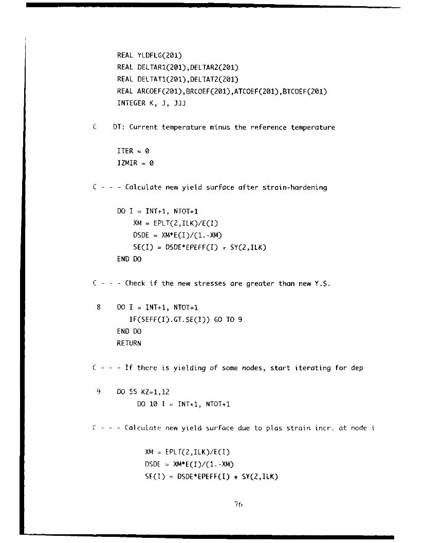
REAL YLDFLG(201)

REAL DELTAR1(201),DELTAR2(201)

REAL DELTAT1(201),DELTAT2(201)

REAL ARCOEF(201),BRCOEF(201),ATCOEF(201),BTCOEF(201)

INTEGER K, J, JJJ

C DT: Current temperature minus the reference temperature

ITER = 0

IZMIR = 0

C - - - Calculate new yield surface after strain-hardening

DO I = INT+1, NTOT+1

XM = EPLT(2,ILK)/E(I)

DSDE = XM*E(I)/(1.-XM)

SE(I) = DSDE*EPEFF(I) , SY(2,ILK)

END DO

C - - - Check if the new stresses are greater than new Y.S.

8 DO I = INT+l, NTOT+1

IF(SEFF(I).GT.SE(I)) GO TO 9

END DO

RETURN

C - - - If there is yielding of some nodes, start iterating for dep

9 DO 55 KZ=1,12

DO 10 1 = INT+l, NTOT+1

COlculate new yield surface due to plas strain incr. at node i

XM = EPLT(2,ILK)/E(I)

DSDI - XM*E(I)/(1,-XM)

SE(1) - DSDE*EPEFF(I) + SY(2,ILK)

76

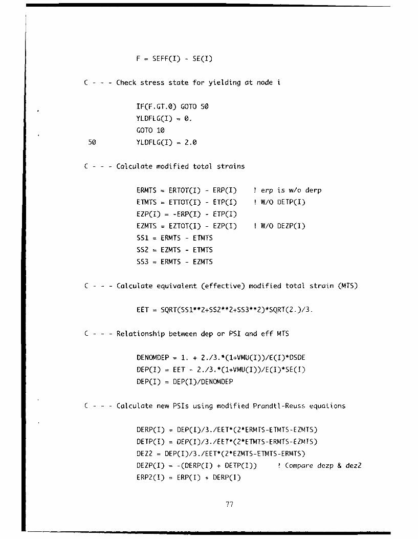
F = SEFF(I) - SE(I)

C - - - Check stress state for yielding at node i

IF(F.GT.0) GOTO 50

YLDFLG(I) = 0.

GOTO 10

50 YLDFLG(I) = 2.0

C - - - Calculate modified total strains

ERMTS =ERTOT(I) - ERP(I) !erp is w/o derp

ETMTS = ETTOT(I) - ETP(I) !W/O DETP(I)

EZP(I) = -ERP(I) - ETP(I)

EZMTS = EZTOT(I) - EZP(I) !W/O DEZP(I)

SS1 =ERMTS - ETMTS

SS2 =EZMTS - ETMTS

SS3 =ERMTS - EZMTS

C - - - Calculate equivalent (effective) modified total strain (MTS)

EET = SQRT(SS1**2+SS2**2+SS3**2)*SQRT(2.)/3.

C - - - Relationship between dep or PSI and eff MTS

DENOMDEP = 1. + 2./3.*(1+VMU(I))/E(I)*DSDE

DEP(I) = FET - 2./3.*(1+VMU(I))/E(I)*SE(I)

DEP(I) = DEP(I)/DENOMDEP

C - - - Calculate new PSIs using modified Prandtl-Reuss equations

DERP(I) = DEP(I)/3./EET*(2*ERMTS-ETMTS-EZMTS)

DETP(I) = DEP(I)/3./EET*(2*ETMTS-ERMTS-EZMTS)

DEZ2 = DEP(I)/3./EET*(2*EZMTS-EThTS-ERMTS)

DEZP(I) = -(DERP(I) + DETP(I)) !Compar'e dezp & dez2

ERP2(I) = ERP(I) + DERP(I)

77

ETP2(I) = ETP(I) + DETP(I)

EZP2(I) = -ERP2(I) - ETP2(I)

FZP2TFST = EZP(I) + DEZP(I)

10 CONTINUE

C - - - Solve O.D.E.s with new plastic strain increments

11 CALL SOLVE(ILK,SR,ST,SZ,SEFF,B,ERP2,ETP2,EZP2)

C - - - Save old plastic strains from the three previous iterations

DO I = INT÷1, NTOT+1

DRTEST1(I) = DRTESTZ(I)

DRTEST2(I) = DRTEST3(I)

DRTEST3(I) = ERP2(I)

DTTEST1(I) = DTTEST2(I)

DTTEST2(I) = DTTEST3(I)

DTTEST3(I) = ETP2(I)

END DO

C --- Faster convergence scheme extrapolates the difference between

C previous plastic strain increments to zero.

IZMIR = IZMIR + 1

IF(IZMIR.EQ.4)THEN

IZMIR = 0

DO 22 1 = INT-e1, NTOT+1

PRODTEST = DRTESTl(I)*DRTEST2(I)*DRTEST3(I)

DRORTEST = ABS(DRTEST2(I)-DRTEST3(I))

DTDTTEST = ABS(DTTEST2(I)-DTTEST3(I))

IF(PRODTEST.NE.0.000000.AND.DRDRTEST.GT.lE-8.AND.

+ DTDTTEST.GT. 1.E-10)THEN

DELTAR1(I) = DRTEST2(I) - DRTEST1(I)

DELTAR2(I) = DRTEST3(I) - DRTEST2(I)

ARCOEF(I) = (DELTAR1(I)-DELTAR2(I))/(DRTEST2(I)-DRTEST3(I))

BRCOEF(I) = DELTAR2(I) -ARCOEF(I)*DRTEST3(I)

78

if(citcoef(i) .gt.le-14)then

ERP2(I) = -BRCOEF(I)/ARCQEF(I)

end if

DELTAT1(I) =DTTEST2(I) - DTTEST1(I)

DELTATZ(I) DTTEST3(I) - DTTEST2(I)

ATCOEF(I) = (DELTAT1(I)-DELTAT2(I))/(DTTEST2(I)-DTTEST3(I))

BTCOEF(I) = DELTAT2(I) -ATCOEF(I)*DTTEST3(I)

if(atcoef(i).gt. le-14)then

ETP2(I) =-BTCOEF(I)/ATCOEF(I)

end if

EZP2(I) =-ERP2(I) - ETPZ(I)

END IF

22 CONTINUE

GOTO 11

END IF

55 CONTINUE

DO M = INT+1, NTOT+1

ERP(M) = ERP2(M)

ETP(M) = ETPZ(M)

EZP(M) = -ERP(M) -ETP(M)

EPEFF(M) = EPEFF(M) + DEP(M)

END DO

RETURN

END

79

C -- - - - - - - - - - - - - - - - - - - - - - - - - - - - - - - - - -

C HEADER LINES FOR THE OUTPUT

C--------------------------------------------------------------------

SUBROUTINE HEADER(NTIME ,TE,PAT,NOT)

REAL TE(20), PAT(20), NOT(20)

WRITE(12, 750)

WRITE(19 ,751)

WRITE(17,752)

WRITE(18 ,753)

750 FORMAT(1X,'STEP ','TEMP ','APPSTRESS ','SEFF ''SR ' ST '

$ ' SZ ',' SY(MPA) ', 'EZMECH')

751 FORMAT(1X,'STEP ,'TEMP ','APPSTRESS ','SZF ' SZM ' SEFFM '

$ 'EEFFM ',' EZMECH ')

75Z FORMAT(1X,'STEP ','TEMP ','ERPM ','ETPM ',' EZPM ',' ERMECH u

$ ' ETMECH ',' EZMECH ', 'ETHERMAL')

753 FORMAT(1X,'R/B ','SEFF ',' SR ',' ST '

$ ' SZ ',' ERP ', vETP ', 'EZP')

RETURN

END

C--------------------------------------------------------------------

C PRINT STRESS OUTPUT IN FDOUTS.DAT AND STRAIN OUTPUT IN FDOUTE.DAT

C--------------------------------------------------------------------

SUBROUTINE OUTS(SEFF,SR,ST,SZ,ILK,NTIME,ERP2,ETPZ,EZP2)

COMMON/MA TO/EF ,EM, CTEF ,CTEM

COMMON/MATi/EC ,E(ZO1) ,VMU(201) ,CTE(Z01) ,R(Z01) ,VF ,EZ

COMMON/MAT3/DT(200) ,T(200) ,ET(5 ,200) ,VMUT(5 ,200), CTET( , 200), P7(200)

COMMON/MA T6/EPL T(5 ,200), SY(5 ,200)

COMMON/LIMITS/NTOT, NRA, INT

COMMON/STRAINS/ERTOT(Z0l), ETTOT(201), EZTOT(201)

COMMON/EMECH/ETHERMAL ,ERMECH,ETMECH,EZMECH

REAL ERP2(201) ,ETP2(201),EZP2(201)

80)

REAL SR(201), ST(201), SZ(201), SEFF(201)

ICYC = ICYC + 1

IF(ICYC .EQ. 1)THEN

WRITE(12,99) NTIME, TE(1), PAT(1)/1.E6, SEFF(1)/1.F6,

+ SR(1)/1.E6, ST(1)/1.E6, SZ(1)/1.E6, SY(2,1)/1.E6,EZMECII

END IF

SS1 = SEFF(INT+1)/1.E6

SSZ = SR(INT+1)/1.E6

SS3 = ST(INT+1)/1.E6

SS4 = SZ(INT+1)/1.E6

SS5 =SY(2,ILK)/1.E6

ETI'ERMAL = CTE(INT+1)*DT(ILK)

ERMECH = ERTOT(INT+1) - ETHERMAL

ETMECH = ETTOT(INT+1) - ETHERMAL

EZMECH = EZTOT(INT+1) - ETHERMAL

WRITE(12,99) NTIME, T(ILK), PZ(ILK)/1.E6, SS1, SS2, SS3, SS4,

+ SS5, EZMECH

L =INT+1

WRITE(17,101) NTIME, T(ILK), ERP2(L), ETP2(L), EZP2(L)

+ , ERMECH, ETMECH, EZMECH, ETHERMAL

99 FORMAT(2X,I4,1X,F7.1,1X,F8.1,1X,5(F8.1,lX),E1O.3)

101 FORMAT(2X,IS,2X,F7.2,7(2X,E11.5))

RETURN

END

81

C -- - - - - - - - - - - - - - - - - - - - - - - - - - - - - - - - - -

C PRINT SUMMARIZED OUTPUT IN FDSUM.DAT

C ------------------------- ------------------------------------------

SUBROUTINE OUTSUM(INT,SZ,SR,ST,SEFF,NTIME,TFIN,PFIN)

COMMQN/STRAINS/ERTOT(201), ETTOT(201), EZTOT(201)

COMMON/EMECH/ETHERMAL ,ERMECH, ETMECH ,EZMECH

REAL SR(201), ST(Z01), SZ(201), SEFF(ZOI)

XSZF = SZ(INT)/1.E6

XSZM = SZ(INT+1)/l.E6

XSEFFM = SEFF(TNT-I-)/l.E6

IZ =INT+1

SQUARE = (ERTOT(IZ)-ETTOT(IZ))**2 + (ERTOT(IZ)-EZTOT(IZ))**2+

+ (ETTOT(IZ)-EZTOT(IZ))**2

XEEFFM = SQRT((SQUARE)*2".'),'3.

XEMECH = EZTOT(INT+1) - ETHERMAL

WRITE(19,222) NTIME, TFIN, PFIN/1.E6,

+ XSZF, XSZM, XSEFFM, XEEFFM, XEMECH

222 FORMAT(16,2(1X,F9.2) ,3(1X,F9.2),2(1X,E12.4))

RETURN

END

C--------------------------------------------------------------------

C PRINT OUTPUT AT THE CROSS-SECTION IN FDUSP.DAT

C--------------------------------------------------------------------

SUBROUTINE OUTUSP(SEFF,SR,ST,SZ,ERP2,ETP2,EZP2,NTOT)

COMMON/MATO/EF ,EM, CTEF ,CTEM

COMMON/MATi/EC ,E(201) ,VMlU(201) ,CTE(201) ,R(201) ,VF ,EZ

REAL ERPZ(201) ,ETP2(201) ,FZP2(201)

REAL SR(201), ST(201), SZ(201), SEFF(201)

DO I=1,NTOT+t

SS1 = SEFF(I)/1.E6

552 = SR(I)/l.E6

82

SS3 = ST(I)/1.E6

SS4 = SZ(I)/1.E6

WRITE(18,88) R(I),SS1,SS2,SS3,SS4,ERP2(I),ETP2(I),EZP2(I)

END DO

88 FORMAT(2X,F7.4,2X,4(F9.2,1X),3(F9.5,1X))

RETURN

END

C ---------------------------------------------------------------------

C COMPUTE RUNTIME

C ---------------------------------------------------------------------

SUBROUTINE REALTIME(NRA,NTIME,XT1)

DELTA = SECNDS(XTI)/60.

WRITE(12,*) 'RUNTIME IS ',DELTA,' MIN FOR ', NRA,' NODES '

$ NTIME, 'TIME INCRS.'

PRINT *, 'RUNTIME IS ',DELTA,' MIN FOR ', NRA,' NODES ',

$ NTIME, 'TIME INCRS.'

RETURN

END

83

APPENDIX BELASTIC SOiUTION OF TWO CONCENTRIC CYLINDERS

Stresses in the matrix and the fiber are given by [281;

arr, = A (1 - -b 2 + P r b r2 , crf = A (1 - -ba 2) - -Pr a-'b .r 2 r,2 a 2 a2

b,2 b2

cr o , = A ( 1 + b 7 P , - -'bc o• = c ¢

r2 r=Ul

b2 b2

,,m = C, Ur¢ =C(1- -b )+ Pý b

a 2 a2

where;

A= S2b 2 (¾uI - U2 S-)+(a,, - af)Tt2SI -- ftS2 a$ 2

t '= - bt 2 -- (ul - U2 ) + (a,,, - af )T- t 2

b12 1 1sl = (I - )- -)a 2 Ef Em'

, b 2 01 + Vft) (1+ V

(12 Ef Em

b 2 2vf 2vm

a2 E, E,b 2 ( + Vf b2 (I+ v.)t2a2 (l E fV 1+ -a 2) E ,

EE Em

u12 = !, - P, +) V P, 0 --V

E) Em

84

APPENDIX CSAMPLE OUTPUT FILES

85

+ I I I I I I I Iui LU LU LULU LU Lu LUJ LU LU

tj() - r400() ' t0o~ eLU()0 t()qtQ )rj-lMr 0 r -.- 4 - 4 jr,

'' (;( * (s, 5) (S, S;(S

(S (S 0)- Y L'

0 + +S + + + + +S +D0()0 ý - - S L y 0()M SDILU LU LU LU LU LU LU) LU LU LU LU) LU LU LU LU0 LU" LU4 LU LU LU0 LU4 LU ý

0 t.0 m m %-

0 (S) 6Cý (S* 6 6 S; (; 14 G 6 (S;6 6ý ý4 4 ý- ýq"i

0 D00()0( DC>mrr Y nr)mmr)r)"r,

ts, - - -(ý!r4r4r- - - ()m Q ()G GL. .. .. .. .. .. .. . . . . ..

0 S D0 D0InSl 0L Itw( -r ) 1 nrjIl

ý414rf - Iý- - q qr4 r fI4. I n m m 4iI mj S r) . . .

N* - - qCt . . . . . . . . . . . . . . ..(s; !D'6 (; 6 (s;0' s; (s> (; 0* (s;(s;6 (; r i L d Y)Gr)'o

r~ r~ I~ I~ I~ I~ (D (S (D IS D()()0C4rir- S oC

+ 11 C1 G \ l l 1 Qrim m() ne e ~)Mr DL+ S (S (S;t~t (S S S S)(;(;(;(;(),(;(IG -:rlriey )'

LUUl ko 00~

(S G S)

(S (S CD m LU - nri 4L l0 N-10r- q0(S D HI'l rjtD0 S)() S 0 r)-4-r rirl t Dr- ~ V .0r . . .

CD P- 0 ) r4 C Y l ~ * - 0 ý r ; r ý c c r: 'l 'tl a' r j (Y) .t

ory CIJ S' It* 4 Lý ý ý L U V LýLAr.1Jr- r- r4 V1 -IT-4r- r- V1 l k D I I I

(S)~~a r (S) (D CO (S SC0()(SG)..L (S 1 D4) S S 0m D000 .

Oý CD ~ L0u nC )< S)"Wrj(>01ý

48 CS)4 4 4 4 !,('. . .U S) . . . . . . .'

+ -4rl -IT- -4rqr- -IV4 - -4q- %ivim a)m m i 0 r L L - - CiM )()86 L 1

Nll N- Ný N ~ N ~ . . ." .N ~ N .N N N N ~ N l N ~ N ~ N N

r- w w I I A I l 0 m t. m 't 00 I- m w m I I LA

LU

(N- re) re) MY rv) re) re) qt- 14- qt -Nt Wt -qt -qt I I- Lr, I~ e)V LA) LA) t.

ýD Lf r'- (D 1-4 N~ rj NT 00Q oo t; 000 oo oo ) N~ f ry 1.o LA LA

0' () N lo 0:0 N ;G;r: S (0 0 8 f'- N - r L(S N- D m i .- 4rIrirIT- - jm tL n, - w 1 0 N 0-i

I NNNN Nj N N,, N,, . N N . N .N N j"c, - lr

,I ()r~ ')V)I t0r- rjLf ) -4C L NJCDm 1ý ) .0r) S4 4 N ')ILrAN L n'r, A L A N o r' n'0-i l'(

O- L) 0 )LAn v ) 1 V.0 LAt0LA0 1 0(n ()d- 1i 4 ko S

(S ** 00 LA) ~oLA 4 r f1(; .4Nv-q, r40400,000*

n N ON rI I4 ri rI I4 r i I- r- I- (N IN rI Iý cI NJ

0

rL A 0l ~ . 00 (>r4r Y) q .0 00 Na .T4 re 1. 0 a) -iL

N- NJý lm nr'-N00O-4N .4 q- - 14-14 A1 ) n 0OLnV)L. M

t.0

(S S ()() D() S S 00 CD0 00)0 CD 0 00 0 CD (S 1.0000 00000000000 0000 SIO .4-

0000000 -* 4 ý ý ý0 4 16 0 G0000 -0SIrý0'... A

F-

87

(n~ rNJ (NJ CNJ (NJ rNJ (NJ "N ('.J "J rNJ (J rNJ rNJ (NJ (NJ (NJ (NJ (NJ C14 "\ (NJ ( -4 r- ,-q ,-i ,-q ~-4 ~-4I I I I II I I I I I I I I I I I I I I I I I I I I I I I I

.. j Uj ULJ LUJ LU LUA LU LUi LUJ LU LUJ LU LU LULU LU LUJ LUJ LUJ LU LU LU LU LUJ LU LU LUJ LU LUJ LUJ LUrn% e l - l - l )0 " ý "a "rla NCiL)riIt( - , ~ y

LU

(S (S J (S> (5) (S) (S) (NJ CD J 0 J (N (N ( (ND (N CD J CD (NJ (S) (S) (N (N (NJ (NJ (NJ (NJ (NJ (NJ (NJ CD

LULLUL LL LLU LU LU LU UL LLU LU LL LULU LU LU LU LU LU LU LU LU LUý LU LU LU LU LU LU1.C 1-tC 00 00 r- m mLi Lfl n LO D t.0 N- C 00 00 (N0 " N " 00 ) (S) Nl fl (n t.0 ry (NJ 1. (SI

LU (S )S( DC

LULU LU LU LU LU LU LU LU LU LU LU LU LL LU LU LU LU ý LU LU LU LU LU LULU LU ý LU LU LU LU(S C-Yr) 0ON~SON 44 WNJm 0r- - L)Nn0 t S 0 I rL 0_0' 0 0 D -jrL D NJ0~ o C0 l _ 4 )m" :V4nIt0) n t o r otk0 "1- -_a T4it 0 -r- c 0G 400 )a Y . 00 n0 0r-ýotot0L )r-0 )" -

LU LULU LUL L LU LU LU LU LU LU LU LU LU LU LU LU LU LU LU LU LU LU LU LU LU LU LU LU LU

M:V 1 - - ~ cti tL)V Dk l l , 00 00 00 oNNNCO0 oO-4.-4 1-4 4LUf . . * I * , . . . . . . . . . . . . . . . . . . . . .

LII IOJN N N JN N N N

+ + + + ++)+ G)11 1 IS I G) I I IS (5 (S (S I ome .j (jr m j c % j(j(LU) LU LUS LU LU LU LU LU LU LU LU LU LU CD LU LU LU LU LU LU LU LU LU) LU LU) LU LU LULUL

0 D(>()C S S D( 4 )m wrt0k 00 t r-rr4N nI(S S )G )C DC S s(~ l 0m00"I*C ~ l )V 0V 0C I()Q0 S S S S D0()( ýC DV - -%DC .r.L qr4()0 oc)rq0 0r

(S D0C D0( S S S - - n("ri(l tk 0a D& ý N n-tV

++ + + + . + +. .+ I I I I I I I I I I I I I I I I I I

LU LU LU LU LU LU LU LU LU LU LU LU LU LU LU LU LU LU LU LU LU LU) LU LU LU LU LU LU LU LU(DC DC DC D0()4 -r_#o0 0U)V 7 l . DN l0 . SCG(S S)0GS () S) S ()(5 ) )00 "N- ) D lm t Z . 10NG Do 252 52 565o2 qa ~ , t16r-o )d 4c44L

0 0 0()()()0 0I)C Dv4tD-4r4r4r4 r ~ , y yI- 6 (;(;(* S S S (;(;6 (;(; 0 sM *(*

0 S ()0G) 5)(S S)0 (S T4v-400~ (D ) 8r- NJ qd L qt ( fl V)W -IG) 0 Gf) 0f N) (SD 0- (S) 0 0 00 Jr4rf"" t. t.tL nL '-4

LUJ (S D (S S G) (* (, *) (SI; ID IS * . . . . .I I I I I I I I I

a_() C S S S S S S 0()0C S )8()0C

000000NNNLImImIm/" NJJNi -4'H-4 r4 00LC1Nrj

LUJ(S - jm ' f . , 0m G - o - f o1-0 -

LL L/l H r, n-tL)o % C lrir4rIr4r4rIrIý lH (J(J" (4r l(ý J" C

88

5 , " rQ I j I ,, I j I j r- -I r r4rI- r-4 I4 r- l -I M CD M (D (D CD (I GI()( (S S

<D 0C D0(D00( ()a a )004D )a D(S D()(S D4 S

m NS NS D()C S DQ DC D0()0()()(ý( S ý0( S DC S DC ý DC S SLU(;(S)() (;(; S*(; S ý 0*(;(S ý6 (S*(;(S S O) S (;6 C')(' (* z, S)S C*C* D S) D *

tD Iý CD Ij ý -l0 ~ f ý r- S) It 0I - 0-DU f f ý 0()r . S f l )C . S -I

CDC S )1-r4a)0000n0i(>00k0L d 1 - ()O 0r . . L d -r)ri(j irI- - S SCDm(S f4 rn I r%% ýrjN 4Cjrirq -lrIrIDiýi()(D( s0 0( Dm( DC 0 m G n (!DI

(S *! (! I)m(SG D() 0( D0D D(Dm(D(>()() S S S ()( S MC S 0DI D

IS IS S L IQ VI In In I.4 4 qt In m In In " I~ I% I~ Cý -4 I I- r4r I r I IS I CD 0 m is CD CD

&L D()()()0G S D() D00C S S S ()( S D()()C D0C

CD0 ()()0C (>()00(>M(S DC D0(ý0G ! S D ()( D()0()C S ! S

(D(w0 S S S S S S S D0 S 0 0 t DCD()()()(l()C ID(,(>()(ý(>(ý(ý(ui 0 D C l I I I I I I I I I I ; I I ; i

re) re) 0 Nrn

00 00 00NN N NN 0000o~~~oo,I 1- I - \ Ir . 0r n0 I tC4r- - ~ ~ Da .w w0 ~ - 0L r

CD0 r ýD 4n r t00 D00q 0 l i r- .-.- e ()LM0 (>ID 0t8,9r r

11 -A( ()G)CD (>G)0 0

0 () S)0 () 0(S 00 00-(D (S (S)(S) () (D(S) D (S>(S> S) (S (S)CD J

(S () D S)(S () S)CDCD(S C C ( C 4

CDCD6 (sCD D*(*r(')f *)(*-(D*(* S (' ()

r~~~~i ~ (S N S>(>0 () S )C C D 0 C

a) -4-rs ( I (S 0 0 (D G) (S I I 0 D IS

0 S ()(S S)C ()(S S)() s ()CD(

(DC N OC C DG)( D S D S 5

(S)(S (S ( (SCS 0 D D C (D SIý C90S.~~~~; -~v a~M~ (S)rN~ (S) (S) (S :D()(S S ( () )C