Effect of rocket exhaust of canisterized missile on ...
13
Original Article Effect of rocket exhaust of canisterized missile on adjoining launching system MSR Chandra Murty, PK Sinha and D Chakraborty Abstract Transient numerical simulations are carried out to study missile motion in a vertical launch system and to estimate the effect of missile exhaust in the adjoining launch structure. Three-dimensional Navier–Stokes equations along with k–" turbulence model and species transport equations are solved using commercial computational fluid dynamics software. Dynamic grid movement is adopted and one degree of freedom trajectory equations are integrated with the computational fluid dynamic solver to obtain the instantaneous position of the missile. Multi-zone grid generation approach with sliding interface method through layering technique is adopted to address the changing boundary problem. The computational methodology is applied to study the missile motion in a scale-down test configuration as well as in the flight condition. The computations capture all essential flow features of test and flight conditions in active cell as well as in adjacent cells. Parametric studies are conducted to study the effect geometrical features and measurement uncertainty in the input data. Computed pressures in the adjacent cells in the launch system match better (12%) with the experimental and flight results compared to distant cells. Keywords Universal vertical launch system, computational fluid dynamics, muzzle blast wave Date received: 21 December 2015; accepted: 1 July 2016 Introduction Two types of missile launching systems are generally employed in combat ships. In the first type, one or two missiles are put in a launcher which is rotated to point the missile towards the target, and the remaining missiles are stored inside the ship. In the second type of launcher, vertical canisters are employed to store and maintain all the missiles in ready to fire condition. Vertically launched canister- ized missiles are operationally very convenient. Both hot launching and soft launching, and combination of the two are employed to eject the missile from the canister. For the hot launching case, the rocket motor is fired within the canister and the exhaust of rocket motor collected in a gas gathering tank before it is let out in the atmosphere through suitable uptake. Compact Vertical Launch System (VLS) needs to con- tain the initial impact of the rocket jet plume and safely discharge the rocket exhaust gas quickly away from the launch installations during firings of the mis- siles which requires innovative mechanical design and good understanding of exhaust plume characteris- tics. 1–4 In the soft launching case, the hot rocket exhausts are avoided and the missile is pushed from the bottom by high pressure gas from gas generators (GG). 5–8 In combined hot and soft launch option, initial missile movement is achieved through pressure built up from GG and the missile is fired during its motion in the canister. The fluid dynamic process inside and outside the canister is transient in nature. While the flow process inside the canister resembles the pressure wave gener- ation in a closed vessel, the wave structure of the exhaust gases during missile leaving the canister is similar to that of blast wave. Blast wave development process during missile exiting the canister tube is explained by Romine and Edquist 9 and is reproduced in Figure 1. Immediately after missile ejection from the canister, high pressure internal gases expand into the surrounding air and a complex flow field including shocks, contact surfaces, jets, etc. is formed. Although the flow field of the muzzle blast from the gun is studied extensively 10–13 in the literature, the flow field investigations in the canister launched missile is very limited. The blast wave flow field from the gun is mostly axial dominated along the barrel axis, while Proc IMechE Part G: J Aerospace Engineering 0(0) 1–13 ! IMechE 2016 Reprints and permissions: sagepub.co.uk/journalsPermissions.nav DOI: 10.1177/0954410016662064 uk.sagepub.com/jaero Directorate of Computational Dynamics, Defence Research and Development Laboratory, HyderabadIndia Corresponding author: Debasis Chakraborty, Directorate of Computational Dynamics, Defence Research and Development Laboratory, Kanchanbagh P.O., Hyderabad 500058, India. Email: [email protected] at DEFENCE RESEARCH DEV LAB on August 8, 2016 pig.sagepub.com Downloaded from
Transcript of Effect of rocket exhaust of canisterized missile on ...
Original Article
Effect of rocket exhaust of canisterizedmissile on adjoining launching system
MSR Chandra Murty, PK Sinha and D Chakraborty
Abstract
Transient numerical simulations are carried out to study missile motion in a vertical launch system and to estimate the
effect of missile exhaust in the adjoining launch structure. Three-dimensional Navier–Stokes equations along with k–"turbulence model and species transport equations are solved using commercial computational fluid dynamics software.
Dynamic grid movement is adopted and one degree of freedom trajectory equations are integrated with the
computational fluid dynamic solver to obtain the instantaneous position of the missile. Multi-zone grid generation
approach with sliding interface method through layering technique is adopted to address the changing boundary problem.
The computational methodology is applied to study the missile motion in a scale-down test configuration as well as in the
flight condition. The computations capture all essential flow features of test and flight conditions in active cell as well as in
adjacent cells. Parametric studies are conducted to study the effect geometrical features and measurement uncertainty
in the input data. Computed pressures in the adjacent cells in the launch system match better (�12%) with the
experimental and flight results compared to distant cells.
Keywords
Universal vertical launch system, computational fluid dynamics, muzzle blast wave
Date received: 21 December 2015; accepted: 1 July 2016
Introduction
Two types of missile launching systems are generallyemployed in combat ships. In the first type, one ortwo missiles are put in a launcher which is rotatedto point the missile towards the target, and theremaining missiles are stored inside the ship. In thesecond type of launcher, vertical canisters areemployed to store and maintain all the missiles inready to fire condition. Vertically launched canister-ized missiles are operationally very convenient. Bothhot launching and soft launching, and combination ofthe two are employed to eject the missile from thecanister. For the hot launching case, the rocketmotor is fired within the canister and the exhaust ofrocket motor collected in a gas gathering tank beforeit is let out in the atmosphere through suitable uptake.Compact Vertical Launch System (VLS) needs to con-tain the initial impact of the rocket jet plume andsafely discharge the rocket exhaust gas quickly awayfrom the launch installations during firings of the mis-siles which requires innovative mechanical design andgood understanding of exhaust plume characteris-tics.1–4 In the soft launching case, the hot rocketexhausts are avoided and the missile is pushed fromthe bottom by high pressure gas from gas generators(GG).5–8 In combined hot and soft launch option,initial missile movement is achieved through pressure
built up from GG and the missile is fired during itsmotion in the canister.
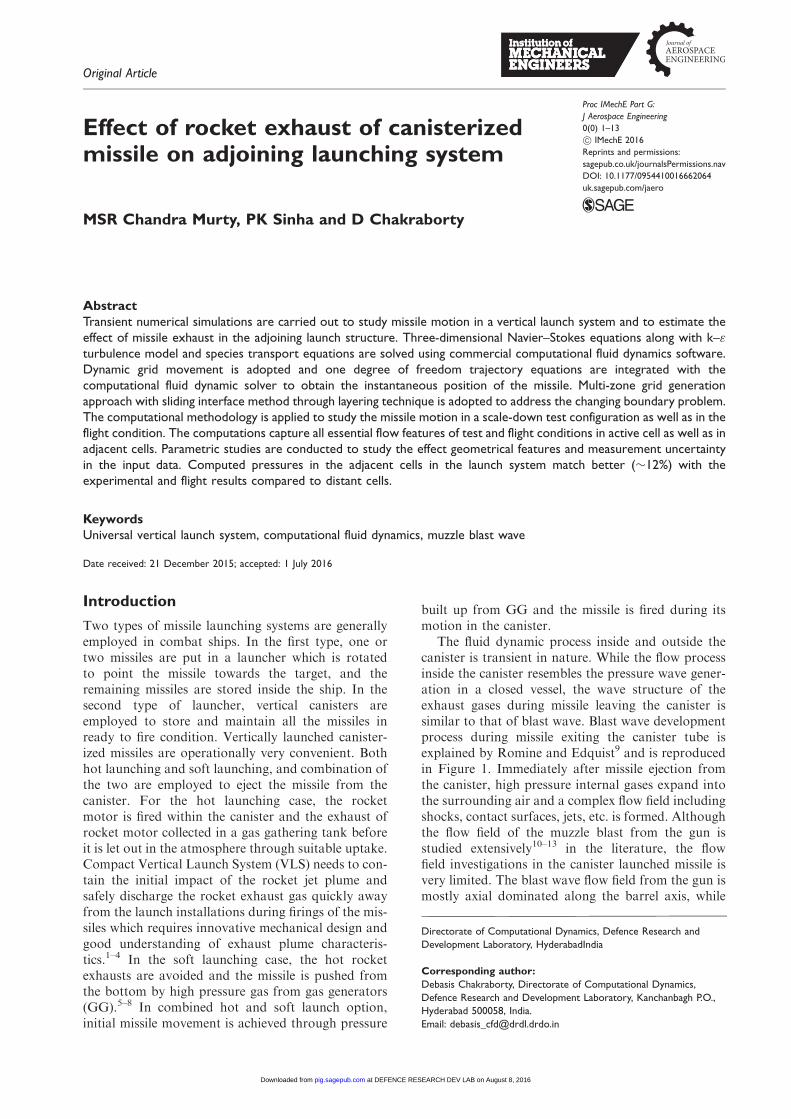
The fluid dynamic process inside and outside thecanister is transient in nature. While the flow processinside the canister resembles the pressure wave gener-ation in a closed vessel, the wave structure of theexhaust gases during missile leaving the canister issimilar to that of blast wave. Blast wave developmentprocess during missile exiting the canister tube isexplained by Romine and Edquist9 and is reproducedin Figure 1. Immediately after missile ejection fromthe canister, high pressure internal gases expand intothe surrounding air and a complex flow field includingshocks, contact surfaces, jets, etc. is formed. Althoughthe flow field of the muzzle blast from the gun isstudied extensively10–13 in the literature, the flowfield investigations in the canister launched missile isvery limited. The blast wave flow field from the gun ismostly axial dominated along the barrel axis, while
Proc IMechE Part G:
J Aerospace Engineering
0(0) 1–13
! IMechE 2016
Reprints and permissions:
sagepub.co.uk/journalsPermissions.nav
DOI: 10.1177/0954410016662064
uk.sagepub.com/jaero
Directorate of Computational Dynamics, Defence Research and
Development Laboratory, HyderabadIndia
Corresponding author:
Debasis Chakraborty, Directorate of Computational Dynamics,
Defence Research and Development Laboratory, Kanchanbagh P.O.,
Hyderabad 500058, India.
Email: [email protected]
at DEFENCE RESEARCH DEV LAB on August 8, 2016pig.sagepub.comDownloaded from
the flow field of canister launched missile is moredependent on the geometry of the opening for gasoutflow. The flow first expands radially outwardthrough the throat formed at the annular openingand axially directed outflow develops when the annu-lar gap exceeds the canister exit area. Till the flowdevelops into axial flow, it is dominated by radialblast wave development process.
Due to flow and geometrical complexities of theproblem, computational fluid dynamic (CFD) meth-ods can be used as an efficient design tool to studymissile ejection from canister. Although good pro-gresses are made in CFD methods including numer-ical algorithms and computing hardware for variousnon-reacting and reacting flow problems, the applica-tions of CFD methods in missile ejection from canis-ter remain very limited. Romine and Edquist9 havestudied numerically the blast wave formation problemfor the missile launched from canister using 2D/axi-symmetric finite difference Eulerian code ‘Shell’.14 Themotion of the solid boundaries within the grid isaccounted for. Lee15 has developed a mathematicalmodel by solving unsteady Euler equations by thefinite difference method based on the method of char-acteristics to simulate the initial transient response ofthe missile launch-tube gas flow and its interactionswith the structural components when the rocketmotor is fired. Numerical solutions compare wellwith the available pressure measurements and theflash X-ray photographs. Liu and Xi8 analyzed thegas dynamics of canister launched missiles usingFluent Software and obtained reasonable matchwith the test data.
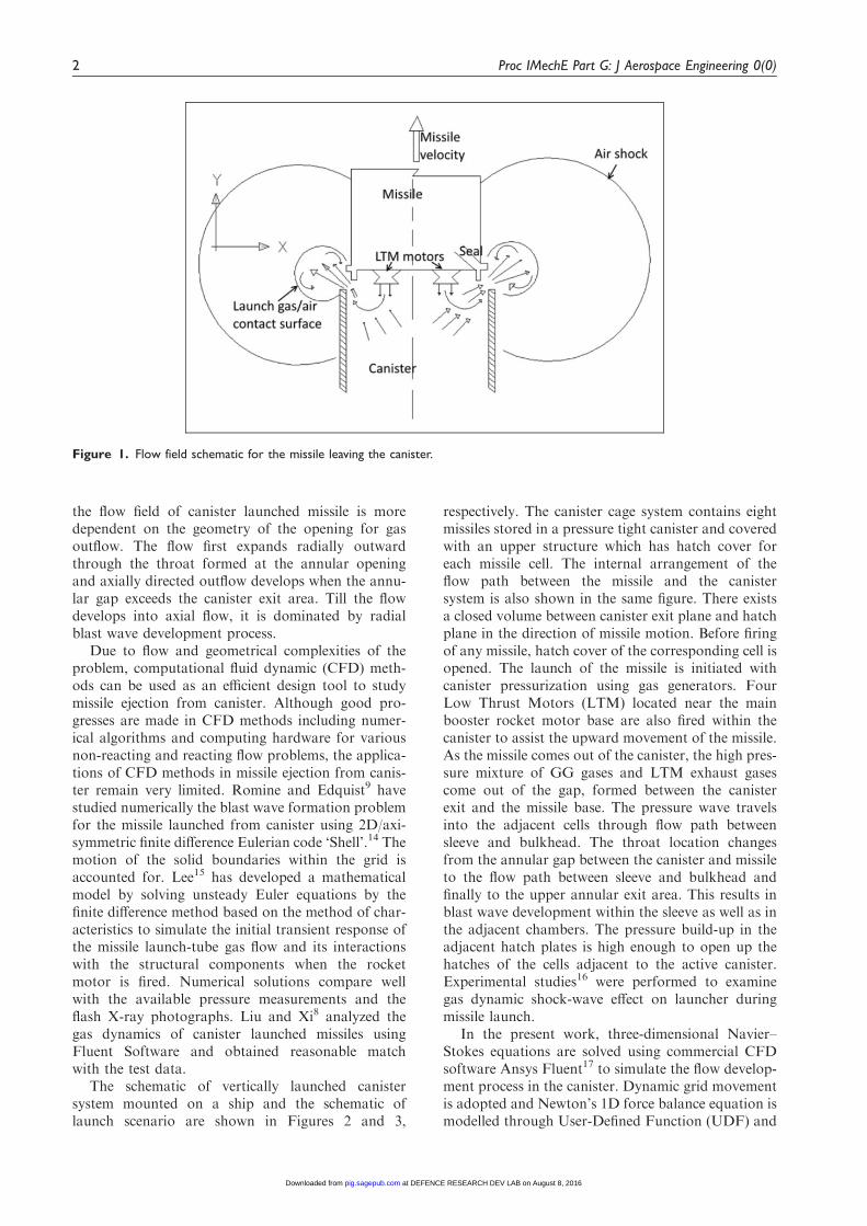
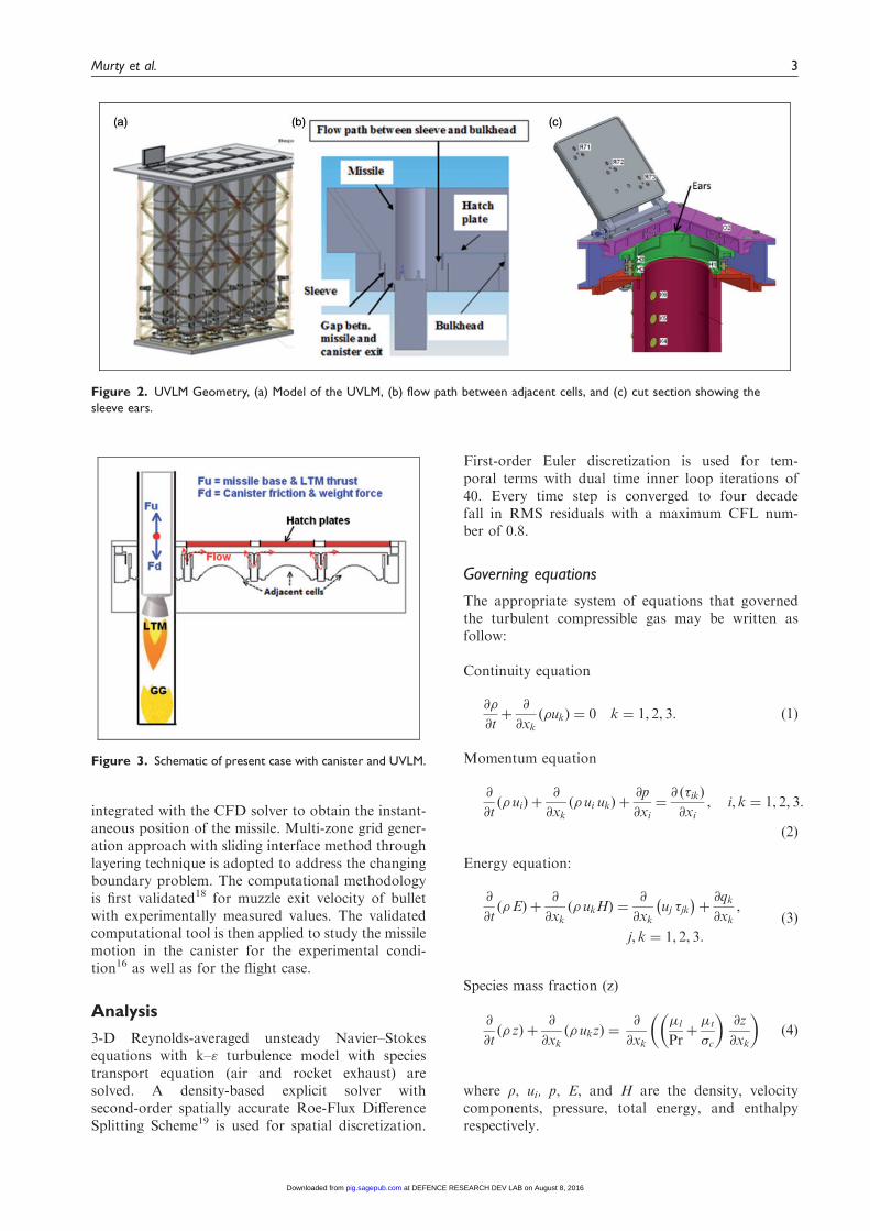
The schematic of vertically launched canistersystem mounted on a ship and the schematic oflaunch scenario are shown in Figures 2 and 3,
respectively. The canister cage system contains eightmissiles stored in a pressure tight canister and coveredwith an upper structure which has hatch cover foreach missile cell. The internal arrangement of theflow path between the missile and the canistersystem is also shown in the same figure. There existsa closed volume between canister exit plane and hatchplane in the direction of missile motion. Before firingof any missile, hatch cover of the corresponding cell isopened. The launch of the missile is initiated withcanister pressurization using gas generators. FourLow Thrust Motors (LTM) located near the mainbooster rocket motor base are also fired within thecanister to assist the upward movement of the missile.As the missile comes out of the canister, the high pres-sure mixture of GG gases and LTM exhaust gasescome out of the gap, formed between the canisterexit and the missile base. The pressure wave travelsinto the adjacent cells through flow path betweensleeve and bulkhead. The throat location changesfrom the annular gap between the canister and missileto the flow path between sleeve and bulkhead andfinally to the upper annular exit area. This results inblast wave development within the sleeve as well as inthe adjacent chambers. The pressure build-up in theadjacent hatch plates is high enough to open up thehatches of the cells adjacent to the active canister.Experimental studies16 were performed to examinegas dynamic shock-wave effect on launcher duringmissile launch.
In the present work, three-dimensional Navier–Stokes equations are solved using commercial CFDsoftware Ansys Fluent17 to simulate the flow develop-ment process in the canister. Dynamic grid movementis adopted and Newton’s 1D force balance equation ismodelled through User-Defined Function (UDF) and
Figure 1. Flow field schematic for the missile leaving the canister.
2 Proc IMechE Part G: J Aerospace Engineering 0(0)
at DEFENCE RESEARCH DEV LAB on August 8, 2016pig.sagepub.comDownloaded from
integrated with the CFD solver to obtain the instant-aneous position of the missile. Multi-zone grid gener-ation approach with sliding interface method throughlayering technique is adopted to address the changingboundary problem. The computational methodologyis first validated18 for muzzle exit velocity of bulletwith experimentally measured values. The validatedcomputational tool is then applied to study the missilemotion in the canister for the experimental condi-tion16 as well as for the flight case.
Analysis
3-D Reynolds-averaged unsteady Navier–Stokesequations with k–" turbulence model with speciestransport equation (air and rocket exhaust) aresolved. A density-based explicit solver withsecond-order spatially accurate Roe-Flux DifferenceSplitting Scheme19 is used for spatial discretization.
First-order Euler discretization is used for tem-poral terms with dual time inner loop iterations of40. Every time step is converged to four decadefall in RMS residuals with a maximum CFL num-ber of 0.8.
Governing equations
The appropriate system of equations that governedthe turbulent compressible gas may be written asfollow:
Continuity equation
@�
@tþ
@
@xk�ukð Þ ¼ 0 k ¼ 1, 2, 3: ð1Þ
Momentum equation
@
@t� uið Þ þ
@
@xk� ui ukð Þ þ
@p
@xi¼@ ð�ikÞ
@xi, i, k ¼ 1, 2, 3:
ð2Þ
Energy equation:
@
@t�Eð Þ þ
@
@xk� ukHð Þ ¼
@
@xkuj �jk� �
þ@qk@xk
,
j, k ¼ 1, 2, 3:
ð3Þ
Species mass fraction (z)
@
@t� zð Þ þ
@
@xk� ukzð Þ ¼
@
@xk
�l
Prþ�t
�c
� �@z
@xk
� �ð4Þ
where q, ui, p, E, and H are the density, velocitycomponents, pressure, total energy, and enthalpyrespectively.
Figure 2. UVLM Geometry, (a) Model of the UVLM, (b) flow path between adjacent cells, and (c) cut section showing the
sleeve ears.
Figure 3. Schematic of present case with canister and UVLM.
Murty et al. 3
at DEFENCE RESEARCH DEV LAB on August 8, 2016pig.sagepub.comDownloaded from
In eddy viscosity models, the stress tensor isexpressed as a function of turbulent viscosity (lt).Based on dimensional analysis, turbulent kineticenergy (K) and turbulent dissipation rate (") aredefined as follow
k ¼ u0iu0i=2 " � �
@u0i@xj
@u0i@xjþ@u0j@xi
� �: ð5Þ
Turbulent kinetic energy (K) equation
@
@t�Kð Þ þ
@
@xk� ukKð Þ ¼
@
@xk
�l
Prþ�t
�K
� �@K
@xk
� �þ SK:
ð6Þ
Rate of dissipation of turbulent kinetic energy (e)equation
@
@t� "ð Þ þ
@
@xk� uk"ð Þ ¼
@
@xk
�l
Prþ�t
�"
� �@"
@xk
� �þ S"
ð7Þ
where l¼llþ lt is the total viscosity; ll, lt being thelaminar and turbulent viscosity and Pr is the Prandtlnumber. The source terms Sk and S" of the K and "equation are defined as
SK ¼ �ik@ui@xk� � " and S" ¼ C"1�ik
@ui@xk� C"2
� "2
K
where the turbulent shear stress is defined as
�ik ¼ �t@ui@xkþ@uk@xi
� �:
Laminar viscosity (ll) is calculated fromSutherland law as
�l ¼ �refT
Tref
� �32Tref þ S
Tþ S
� �
where T is the temperature and lref, Tref and Sare known values. The turbulent viscosity lt iscalculated as
�t ¼ c��K 2
":
The coefficients involved in the calculation of lt aretaken as
c� ¼ 0:09, C"1 ¼ 1:44, C"2 ¼ 1:92�K ¼ 1:0, �" ¼ 1:3, �c ¼ 0:9:
The heat flux qk is calculated as qk ¼ �l @T@xk
, wherel is the thermal conductivity.
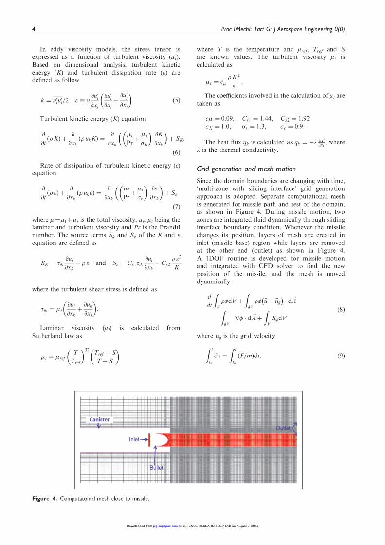
Grid generation and mesh motion
Since the domain boundaries are changing with time,‘multi-zone with sliding interface’ grid generationapproach is adopted. Separate computational meshis generated for missile path and rest of the domain,as shown in Figure 4. During missile motion, twozones are integrated fluid dynamically through slidinginterface boundary condition. Whenever the missilechanges its position, layers of mesh are created ininlet (missile base) region while layers are removedat the other end (outlet) as shown in Figure 4.A 1DOF routine is developed for missile motionand integrated with CFD solver to find the newposition of the missile, and the mesh is moveddynamically.
d
dt
ZV
��dVþ
Z@V
�� ~u� ~ug� �
� d ~A
¼
Z@V
�r� � d ~Aþ
ZV
S�dV
ð8Þ
where ug is the grid velocity
Z t
to
dv ¼
Z t
to
ðF=mÞdt: ð9Þ
Figure 4. Computatoinal mesh close to missile.
4 Proc IMechE Part G: J Aerospace Engineering 0(0)
at DEFENCE RESEARCH DEV LAB on August 8, 2016pig.sagepub.comDownloaded from
Here, F is the resultant force acting on missile,including pressure force on missile base, LTMthrust, gravity force, and drag force. m is instantan-eous missile mass corrected with exhausted propelledgas.
The instantaneous missile velocity is obtained asfollows
vt ¼ vt��t þ ðF=mÞ�t: ð10Þ
In the CFD solver,17 dynamic meshing is imple-mented through layering. According to this method,a computational cell is split into two, if the size of thecell (h) meets the criteria h> (1þ as) hideal. Similarly,two adjacent cells collapse into single cell upon meet-ing the criteria h <ac hideal (see Figure 5). as and ac arethe split factor and collapse factor. The values ofhideal, as, and ac are determined by trial and errortill the solution stabilizes. As the flow gradient is ini-tially high and reduces subsequently, the above par-ameters are checked for the stability of the solution ofinitial motion. Further simulation is done by fixingthese parameters for a given problem.
Simulation of scale-downtest configuration
Description of experimental setup
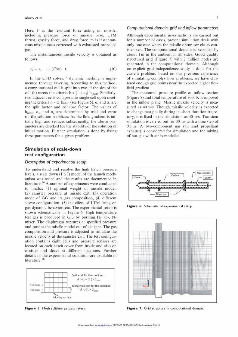
To understand and resolve the high hatch pressurelevels, a scale down (1:6.7) model of the launch mech-anism was tested and the results are documented inliterature.16 A number of experiments were conductedto finalize (1) optimal weight of missile model,(2) canister pressure at missile exit, (3) operationmode of GG and its gas composition, (4) differentsleeve configuration, (5) the effect of LTM firing ongas dynamic behavior, etc. The experimental setup isshown schematically in Figure 6. High temperaturetest gas is produced in GG by burning H2, O2, N2
mixer. The diaphragm ruptures at specified pressureand pushes the missile model out of canister. The gascomposition and pressure is adjusted to simulate themissile velocity at the canister exit. The test configur-ation contains eight cells and pressure sensors arelocated on each hatch cover from inside and also oncanister and sleeve at different locations. Furtherdetails of the experimental condition are available inliterature.16
Computational domain, grid and inflow parameters
Although experimental investigations are carried outfor a number of cases, present simulation deals withonly one case where the missile obturator clears can-ister exit. The computational domain is extended byabout 1m in the ambient in all sides. Good qualitystructured grid (Figure 7) with 2 million nodes aregenerated in the computational domain. Althoughno explicit grid independence study is done for thecurrent problem, based on our previous experienceof simulating complex flow problems, we have clus-tered enough grid points near the expected higher flowfield gradient.
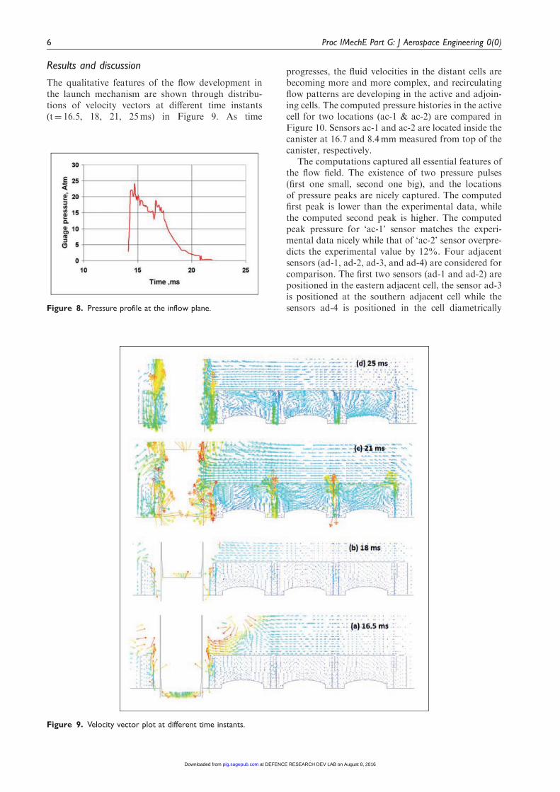
The measured pressure profile at inflow section(Figure 8) and total temperature of 3000K is imposedin the inflow plane. Missile muzzle velocity is mea-sured as 40m/s. Though missile velocity is expectedto change marginally during its short duration trajec-tory, it is fixed in the simulation as 40m/s. Transientsimulation is carried out for 30ms with a time step of0.1ms. A two-component gas (air and propellantexhaust) is considered for simulation and the mixingof hot gas with air is modelled.
Figure 5. Mesh split/merge parameters.
Figure 6. Schematic of experimental setup.
Figure 7. Grid structure in computational domain.
Murty et al. 5
at DEFENCE RESEARCH DEV LAB on August 8, 2016pig.sagepub.comDownloaded from
Results and discussion
The qualitative features of the flow development inthe launch mechanism are shown through distribu-tions of velocity vectors at different time instants(t¼ 16.5, 18, 21, 25ms) in Figure 9. As time
progresses, the fluid velocities in the distant cells arebecoming more and more complex, and recirculatingflow patterns are developing in the active and adjoin-ing cells. The computed pressure histories in the activecell for two locations (ac-1 & ac-2) are compared inFigure 10. Sensors ac-1 and ac-2 are located inside thecanister at 16.7 and 8.4mm measured from top of thecanister, respectively.
The computations captured all essential features ofthe flow field. The existence of two pressure pulses(first one small, second one big), and the locationsof pressure peaks are nicely captured. The computedfirst peak is lower than the experimental data, whilethe computed second peak is higher. The computedpeak pressure for ‘ac-1’ sensor matches the experi-mental data nicely while that of ‘ac-2’ sensor overpre-dicts the experimental value by 12%. Four adjacentsensors (ad-1, ad-2, ad-3, and ad-4) are considered forcomparison. The first two sensors (ad-1 and ad-2) arepositioned in the eastern adjacent cell, the sensor ad-3is positioned at the southern adjacent cell while thesensors ad-4 is positioned in the cell diametricallyFigure 8. Pressure profile at the inflow plane.
Figure 9. Velocity vector plot at different time instants.
6 Proc IMechE Part G: J Aerospace Engineering 0(0)
at DEFENCE RESEARCH DEV LAB on August 8, 2016pig.sagepub.comDownloaded from
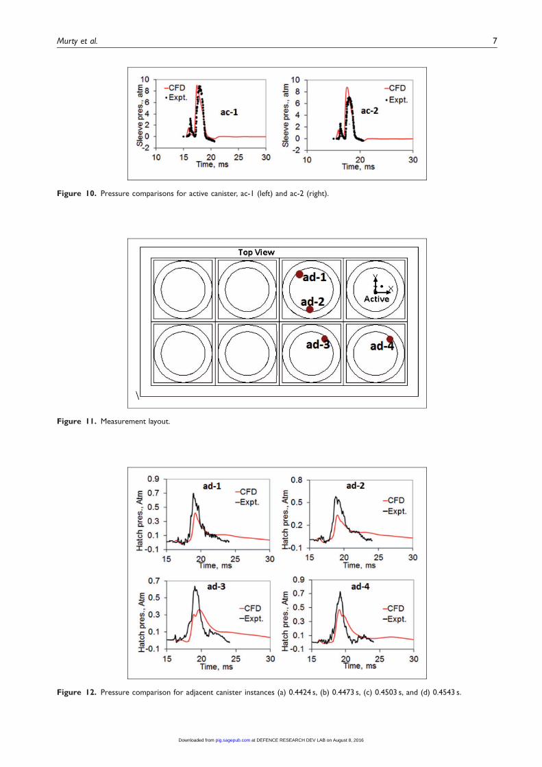
Figure 10. Pressure comparisons for active canister, ac-1 (left) and ac-2 (right).
Figure 11. Measurement layout.
Figure 12. Pressure comparison for adjacent canister instances (a) 0.4424 s, (b) 0.4473 s, (c) 0.4503 s, and (d) 0.4543 s.
Murty et al. 7
at DEFENCE RESEARCH DEV LAB on August 8, 2016pig.sagepub.comDownloaded from
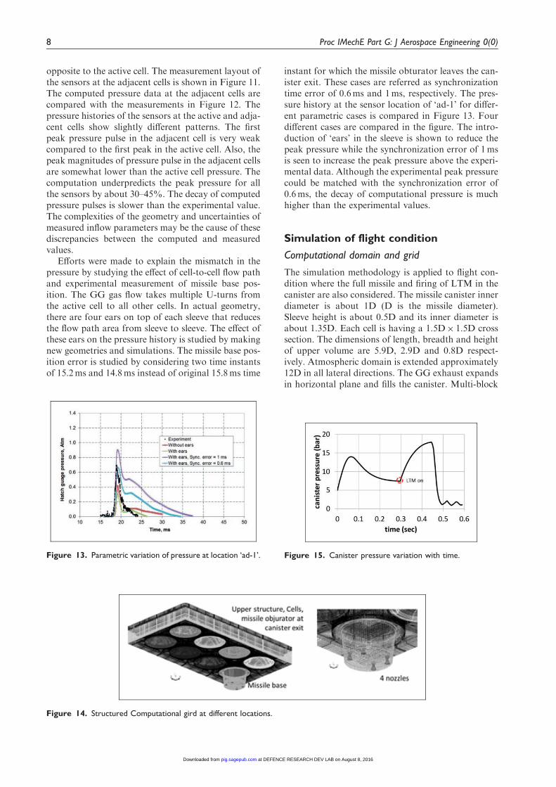
opposite to the active cell. The measurement layout ofthe sensors at the adjacent cells is shown in Figure 11.The computed pressure data at the adjacent cells arecompared with the measurements in Figure 12. Thepressure histories of the sensors at the active and adja-cent cells show slightly different patterns. The firstpeak pressure pulse in the adjacent cell is very weakcompared to the first peak in the active cell. Also, thepeak magnitudes of pressure pulse in the adjacent cellsare somewhat lower than the active cell pressure. Thecomputation underpredicts the peak pressure for allthe sensors by about 30–45%. The decay of computedpressure pulses is slower than the experimental value.The complexities of the geometry and uncertainties ofmeasured inflow parameters may be the cause of thesediscrepancies between the computed and measuredvalues.
Efforts were made to explain the mismatch in thepressure by studying the effect of cell-to-cell flow pathand experimental measurement of missile base pos-ition. The GG gas flow takes multiple U-turns fromthe active cell to all other cells. In actual geometry,there are four ears on top of each sleeve that reducesthe flow path area from sleeve to sleeve. The effect ofthese ears on the pressure history is studied by makingnew geometries and simulations. The missile base pos-ition error is studied by considering two time instantsof 15.2ms and 14.8ms instead of original 15.8ms time
instant for which the missile obturator leaves the can-ister exit. These cases are referred as synchronizationtime error of 0.6ms and 1ms, respectively. The pres-sure history at the sensor location of ‘ad-1’ for differ-ent parametric cases is compared in Figure 13. Fourdifferent cases are compared in the figure. The intro-duction of ‘ears’ in the sleeve is shown to reduce thepeak pressure while the synchronization error of 1msis seen to increase the peak pressure above the experi-mental data. Although the experimental peak pressurecould be matched with the synchronization error of0.6ms, the decay of computational pressure is muchhigher than the experimental values.
Simulation of flight condition
Computational domain and grid
The simulation methodology is applied to flight con-dition where the full missile and firing of LTM in thecanister are also considered. The missile canister innerdiameter is about 1D (D is the missile diameter).Sleeve height is about 0.5D and its inner diameter isabout 1.35D. Each cell is having a 1.5D� 1.5D crosssection. The dimensions of length, breadth and heightof upper volume are 5.9D, 2.9D and 0.8D respect-ively. Atmospheric domain is extended approximately12D in all lateral directions. The GG exhaust expandsin horizontal plane and fills the canister. Multi-block
Figure 13. Parametric variation of pressure at location ‘ad-1’.
Figure 14. Structured Computational gird at different locations.
Figure 15. Canister pressure variation with time.
8 Proc IMechE Part G: J Aerospace Engineering 0(0)
at DEFENCE RESEARCH DEV LAB on August 8, 2016pig.sagepub.comDownloaded from
structured grid of about 2 million cells is generatedin the computational domain at the start of thesimulation. The grid distributions at upper structureand at the missile with four LTM nozzles are
depicted at Figure 14. As the missile moves withtime, domain boundaries change with time. Gridsize goes on increasing as time proceeds, due to add-ition of grid layers at the bottom of the missile.
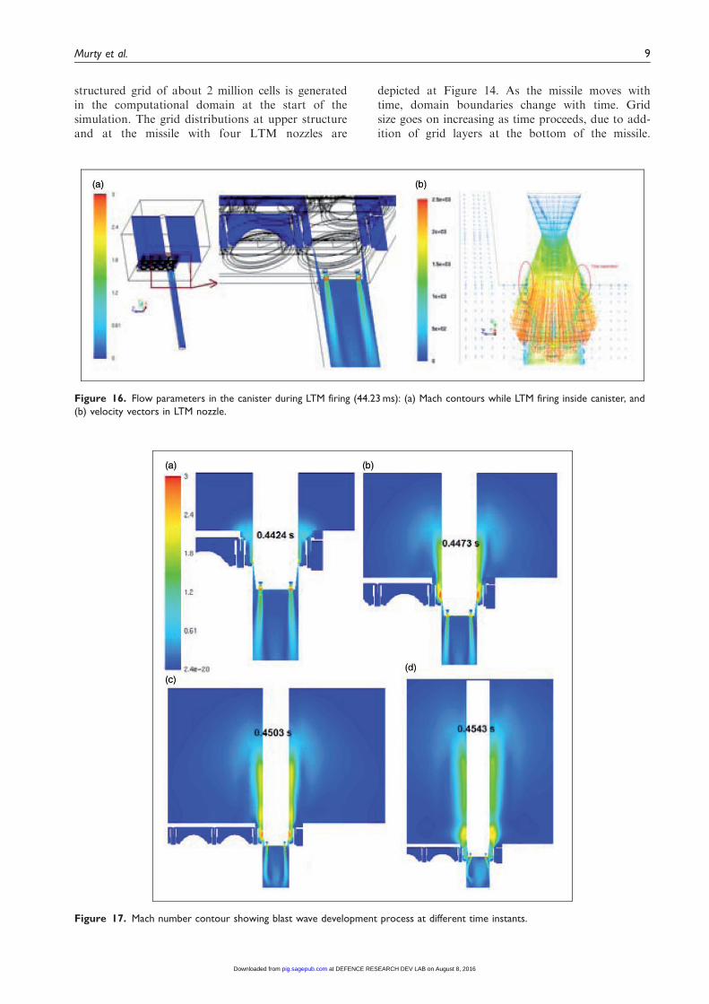
Figure 16. Flow parameters in the canister during LTM firing (44.23 ms): (a) Mach contours while LTM firing inside canister, and
(b) velocity vectors in LTM nozzle.
Figure 17. Mach number contour showing blast wave development process at different time instants.
Murty et al. 9
at DEFENCE RESEARCH DEV LAB on August 8, 2016pig.sagepub.comDownloaded from
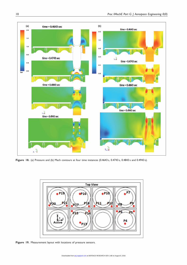
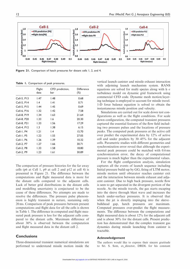
Figure 18. (a) Pressure and (b) Mach contours at four time instances (0.4643 s, 0.4743 s, 0.4843 s and 0.4943 s).
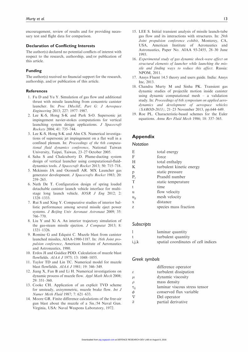
Figure 19. Measurement layout with locations of pressure sensors.
10 Proc IMechE Part G: J Aerospace Engineering 0(0)
at DEFENCE RESEARCH DEV LAB on August 8, 2016pig.sagepub.comDownloaded from

The final grid size is about 4.6 million at the end of thesimulation time.
Results and discussions
Four different events of launch sequence, namely (a) ini-tial pressure build-up by GG to start the missilemotion, (b) missile motion till LTM motors start oper-ating, (c) missile motion until obturator reaches canis-ter exit, and (d) obturator opens to atmosphere causingactive and adjacent canister flow interaction, areaddressed in the simulation. Nitrogen gas is injectedinto the canister at temperature of 300K for about12.3ms. The missile base pressure reached about 7.83bar and missile starts moving forward in the canister.In the second phase, missile movement is modelled by1DOF force balance equation and the missile is movedtill 0.2962 s till LTM is fired. Volume-averaged canisterpressure history is plotted in Figure 15. Canister pres-sure increased to about 14 bar at 0.6 s, and slowlyreduces to about 7.5 bar by the end of the secondphase when the missile attains the velocity of about22.5m/s. At 0.2962 s, LTM are fired and the missileexperiences additional thrust and accelerates further.Canister pressure rapidly increases to about 17.8 bar(see Figure 15) and the obturator reaches canister exitat 0.4423 s.
Mach number distribution in the canister duringLTM firing (at 0.4423 s) is shown in Figure 16. Withthe expansion of LTM nozzle flow, mixing with can-ister gas is clearly observed. Due to high back pres-sure, nozzle flow gets separated in the divergentportion of the nozzle (Figure 16 (b)). As the missiletravels, the gas starts escaping into the sleeve throughblast wave and the canister pressure starts falling. TheMach number contour around canister exit is shownin Figure 17 at four instances depicting the blast wavemovement.
Missile base clears the canister exit at 0.453 s andthe combined canister and LTM nozzle flow interactwith upper structure (TSS), and in this phase thehatches get exposed to the canister flow. The highpressure and high temperature gas enter into thegaps between sleeves and bulk head structure by
taking multiple U-turns and increase the hatchunder-surface pressures. The snapshots of Machnumber and pressure distribution in the active cellas well as in the adjacent top structure at differenttime instants (46.4, 47.4, 48.4 and 49.4ms) areshown in Figure 18. In the contour plots, the relativechange in missile position with time is also observed.At time 0.4432 s, obturator just opens to atmosphere,and slowly the annular gap increases with time, and at0.453 s, the missile base reaches the canister exit. By0.464 s, the missile base reaches the top of the TSS. Bythe end of 0.494 s, the missile has reached a height ofabout 1.9m from canister exit. Pressure is seen to riseon the hatch under-surface around 0.464 s time due tointeraction of two opposing jets (LTM jet and canisterjet) causing the diversion of flow towards sleeve–bulkhead gap. Though the pressures are high duringthe period it travels from canister exit to upper volumeexit plane (0.453< t< 0.464 s), the resultant side jet isnot diverted towards sleeve-bulkhead gap due to pres-ence of sleeve and expands to atmosphere. But, after0.464 s, the incident angle of resultant jet is diverted tosleeve–bulkhead gap, thus causing the hatch pressurerise. We can also observe from contour plots that theresultant jet angle undergoes changes with position ofmissile. It is clearly observed that at around 0.47 s, thejet is directly impinging into the sleeve–bulkhead gap,and thus causes the maximum hatch pressures. Thishigh pressure under the hatch cover plates caused thefailure of latch mechanism and broke open the hatchcover plates in the initial flight trials.
Number of pressure sensors was provided in theadjacent cells of the launch mechanism to estimatethe interaction of canister exit gas. The schematic ofpressure sensors’ locations is provided in Figure 19.The computed pressure history of the adjacent cells(p13 at cell 5, p16 at cell 6 and p22 at cell8) is com-pared with flight data in Figure 20 and a reasonablegood match is obtained. Although computed pres-sures capture the trend of the flight measured data,it is over-predicted compared to the flight measure-ments. However, at 0.464 s, when the missile baseclears the TSS upper surface, the computationand flight measured data is closely matching.
Figure 20. Comparison of hatch pressures for adjacent cells (cells 5, 6, and 8).
Murty et al. 11
at DEFENCE RESEARCH DEV LAB on August 8, 2016pig.sagepub.comDownloaded from
The comparison of pressure histories for the far awaycells (p6 at Cell 1, p9 at cell 2 and p12 at cell 4) ispresented in Figure 21. The difference between thecomputations and flight measured data is more forthe distant cells compared to the adjacent cells.Lack of better grid distributions in the distant cellsand modelling uncertainty is conjectured to be thecause of these differences. No attempts are made toresolve the differences. The pressure pulse phenom-enon is highly transient in nature, sustaining only20ms. Comparison of peak pressures between presentcomputations and flight data for all the cells is shownin Table 1. The difference in computed and flight mea-sured peak pressure is less for the adjacent cells com-pared to the distant cells. Maximum difference ofabout 30% is observed between the computationand flight measured data in the distant cell 2.
Conclusions
Three-dimensional transient numerical simulations areperformed to understand missile motion inside the
vertical launch canister and missile exhaust interactionwith adjoining launch mechanism system. RANSequations are solved for multi species along with k–"turbulence model on dynamic grid framework usingcommercial CFD code. Dynamic mesh motion/layer-ing technique is employed to account for missile travel.1-D force balance equation is solved to obtain theinstantaneous missile position and velocity.
Simulations are carried out for scale down test con-figurations as well as the flight conditions. For scaledown configuration, the computed transient pressurescaptured the essential features of the flow field includ-ing two pressure pulses and the locations of pressurepeaks. The computed peak pressures at the active cellover predict the experimental data by 12% of activecell and under predicts by 30–45% for the adjacentcells. Parametric studies with different geometries andsynchronization error reveal that although the experi-mental peak pressure could be matched with 0.6mssynchronization error, the decay of computationalpressure is much higher than the experimental values.
For the flight configuration analysis, simulationcaptures all the events of launch sequence includingInitial pressure build-up by GG, firing of LTMmotor,missile motion until obturator reaches canister exitand the interaction between missile exhaust and adja-cent canister. Due to high back pressure, nozzle flowis seen to get separated in the divergent portion of thenozzle. As the missile travels, the gas starts escapinginto the sleeve through blast wave and increases thehatch under-surface pressures. It is observed thatwhen the jet is directly impinging into the sleeve–bulkhead gap, hatch pressures are maximum.Computed pressures over-predict the flight measure-ments. The difference between the computations andflight measured data is about 12% for the adjacent celland is about 30% for the distant cells. Present predic-tion has demonstrated that the complex transient gasdynamics during missile launching from canister istractable.
Acknowledgement
The authors would like to express their sincere gratitudeto Sri. S. Som, ex_director, DRDL for his constant
Figure 21. Comparison of hatch pressures for distant cells 1, 2, and 4.
Table 1. Comparison of peak pressures.
Flight
data
CFD prediction,
bar
Difference
(%)
Cell-5, P13 1.47 1.48 0.68
Cell-5, P14 1.4 1.41 0.71
Cell-5, P15 1.44 1.45 0.69
Cell-6, P16 1.32 1.42 7.58
Cell-8, P19 1.34 1.63 21.64
Cell-8, P20 1.33 1.6 20.30
Cell-8, P21 1.33 1.56 17.29
Cell-4, P12 1.3 1.38 6.15
Cell-1, P4 1.21 1.4 15.70
Cell-1, P5 1.22 1.55 27.05
Cell-1, P6 1.26 1.39 10.32
Cell-2, P7 1.27 1.66 30.71
Cell-2, P8 1.33 1.58 18.80
Cell-2, P9 1.23 1.61 30.89
12 Proc IMechE Part G: J Aerospace Engineering 0(0)
at DEFENCE RESEARCH DEV LAB on August 8, 2016pig.sagepub.comDownloaded from
encouragement, review of results and for providing neces-sary test and flight data for comparison.
Declaration of Conflicting Interests
The author(s) declared no potential conflicts of interest with
respect to the research, authorship, and/or publication ofthis article.
Funding
The author(s) received no financial support for the research,
authorship, and/or publication of this article.
References
1. Fu D and Yu Y. Simulation of gas flow and additionalthrust with missile launching from concentric canister
launcher. In: Proc IMechE, Part G: J AerospaceEngineering 2013; 227: 1977–1987.
2. Lee K-S, Hong S-K and Park S-O. Supersonic jet
impingement navier-stokes computations for verticallaunching system design applications. J SpacecraftRockets 2004; 41: 735–744.
3. Lee K-S, Hong S-K and Ahn CS. Numerical investiga-tions of supersonic jet impingement on a flat wall in aconfined plenum. In: Proceedings of the 6th computa-
tional fluid dynamics conference, National TaiwanUniversity, Taipei, Taiwan, 23–27 October 2005.
4. Saha S and Chakraborty D. Plume-ducting systemdesign of vertical launcher using computational-fluid-
dynamics tools. J Spacecraft Rocket 2013; 50: 715–718.5. Mckinnis JA and Oconnell AR. MX Launcher gas
generator development. J Spacecrafts Rocket 1983; 20:
259–265.6. Nath De T. Configuration design of spring loaded
detachable canister launch vehicle interface for multi-
stage long launch vehicle. IOSR J Eng 2012; 2:1328–1333.
7. Rui S and Xing Y. Comparative studies of interior bal-listic performance among several missile eject power
systems. J Beijing Univ Aeronaut Astronaut 2009; 35:766–770.
8. Liu Y and Xi A. An interior trajectory simulation of
the gas-steam missile ejection. J Computat 2013; 8:1321–1326.
9. Romine G and Edquist C. Muzzle blast from canister
launched missiles, AIAA-1980-1187. In: 16th Joint pro-pulsion conference, American Institute of Aeronauticsand Astronautics, 1980.
10. Erdos JI and Guidice PDD. Calculation of muzzle blastflowfields. AIAA J 1975; 13: 1048–1055.
11. Taylor TD and Lin TC. Numerical model for muzzleblast flowfields. AIAA J 1981; 19: 346–349.
12. Jiang X, Fan B and Li H. Numerical investigations ondynamic process of muzzle flow. Appl Math Mech 2008;29: 351–360.
13. Cooke CH. Application of an explicit TVD schemefor unsteady, axisymmetric, muzzle brake flow. Int JNumer Meth Fluid 1987; 7: 621–633.
14. Moore GR. Finite difference calculations of the free-airgun blast about the muzzle of a 5in./54 Naval Gun.Virginia, USA: Naval Weapons Laboratory, 1972.
15. LEE S. Initial transient analysis of missile launch-tubegas flow and its interactions with structures. In: 29thJoint propulsion conference exhibit, Monterey, CA,
USA, American Institute of Aeronautics andAstronautics, Paper No. AIAA 93-2455, 28–30 June1993.
16. Experimental study of gas dynamic shock-wave affect onstructural elements of launcher while launching the mis-sile and finding ways to reduce this affect. Russia:
NPOM, 2011.17. Ansys Fluent 14.5 theory and users guide. India: Ansys
Inc, 2013.18. Chandra Murty M and Sinha PK. Transient gas
dynamic studies of projectile motion inside canisterusing dynamic computational mesh – a validationstudy. In: Proceedings of 6th symposium on applied aero-
dynamics and development of aerospace vehicles(SAROD-2013), 21–23 November 2013, pp.644–649.
19. Roe PL. Characteristic-based schemes for the Euler
equations. Annu Rev Fluid Mech 1986; 18: 337–365.
Appendix
Notation
E total energyF forceH total enthalpyK turbulent kinetic energyp static pressurePr Prandtl numberT static temperaturet timeu flow velocityug mesh velocityx distancez species mass fraction
Subscripts
l laminar quantityt turbulent quantityi,j,k spatial coordinates of cell indices
Greek symbols
� difference operator" turbulent dissipation� dynamic viscosity� mass densitysij laminar viscous stress tensor� conserved flux variabler Del operator@ partial derivative
Murty et al. 13
at DEFENCE RESEARCH DEV LAB on August 8, 2016pig.sagepub.comDownloaded from