Effect of ambiguities in loop cosmology onprimordial power spectrum

Parampreet Singh

Department of Physics & AstronomyLouisiana State University

ILQGS(Feb 5, 2019)

Based on work with Bao-Fei Li and Anzhong Wang (arXiv:1912.08225)

1 / 24

Outline

Introduction

Ambiguities in background dynamics resulting from differentregularizations of Hamiltonian constraint – modified loopquantum cosmologies: mLQC-I, mLQC-II

Ambiguity in choice of momentum of the scale factor in theHamiltonian for scalar perturbations

Comparison of primordial power spectrum in different modelswith initial conditions imposed in the contracting branch

Summary

Goal: What is the effect of different ambiguities on the primordialscalar/tensor power spectrum in different regimes?

Caveat: Assuming validity of dressed metric approach asunderstood in LQC so far for modified LQC models.

2 / 24

IntroductionInflationary paradigm resolves several puzzles in the standardcosmological model. Provides a framework to explain theformation of large scale cosmic structure in the universe.

But, inflation is past incomplete (Borde, Guth, Vilenkin (03)). Quantumgravity expected to resolve big bang singularity and provide aPlanck scale extension of the inflationary paradigm.

Such a non-singular extension exists in LQC (Agullo, Ashtekar, Nelson (12)).Existence of attractors for isotropic as well as anisotropic LQC(Barrau, Gupt, Linsefors, Martineau, PS, Ranken, Schander, Vandersloot, Vereshchagin (07-16)).Inflation natural in LQC (Ashtekar, Corichi, Karami, Sloan (10-13)).

QG effects not washed out by inflation. Non Bunch-Davies vacuumstates at onset of inflation result in stimulated particle creationleading to departures from GR (Agullo, Navarro-Salas, Parker (11))

Non-trivial pre-inflationary dynamics potentially provides a windowto observe quantum gravity effects in CMB.

3 / 24

LQC and perturbationsIn the last decade, cosmological perturbations in LQC exploredusing different approaches (Agullo, Ashtekar, Barrau, Bojowald, Bolliet, Bonga, Cleaver, De

Blas, F-Mendez, Gomar, Grain, Gupt, Hossain, Kagan, Kirsten, Li, Marugan, M-Benito, F-Mendez, Mielczarek,

Morris, Nelson, Olmedo, Shankaranarayanan, Sheng, Sreenath, Vidotto, Wang, Wilson-Ewing, Zhu, ... (08-..))

Dressed metric (Agullo, Ashtekar, Nelson (13)) and the hybrid approach (Gomar,

M-Benito, F-Mendez, Marugan, Olemdo (13)) have gained most attention recently.Both utilize Fock quantized perturbations over loop quantizedbackground. Qualitative results in agreement.

Quite non-trivial that results agree with standard cosmology whileproviding a window to test LQC effects. Many interesting noveland robust results, which include:

Suppression of power for ` ≤ 30 for a choice of initial states(De Blas, Olmedo (16); Ashtekar, Gupt (17))

Signatures in non-gaussianities due to bounce(Agullo, Bolliet, Sreenath (18))

Overcoming tension in CMB data concerning power anomalyand lensing amplitude (Ashtekar, Gupt, Jeong, Sreenath (20)) 4 / 24

Dressed metric approach (Agullo, Ashtekar, Nelson (13))

Based on QFT on quantum spacetimes (Ashtekar, Kaminski, Lewandowski (09)).Quantum state of form: ψ0 ⊗ ψ1 with −i~∂φψ0(v, φ) = H0ψ0(v, φ) andψ1(Q,T, φ) is such that backreaction of perturbations onbackground is negligible (test-field approximation).

Dynamics of ψ1(Q,T, φ) is completely equivalent to that of a stateevolving on an metric “dressed” with QG corrections

gabdxadxb = a

(−dη2 + dxidx

i)

where

a4 = 〈H−1/20 a4H

−1/20 〉

〈H−10 〉

, dη =(〈H−1

0 〉〈H−1/20 a4H

−1/20 〉

)1/2dφ

Expectation values computed using sharply peaked ψ0 states.

Assumptions in our analysis: We consider sharply peaked states oneffective geometry. We assume implications from subtle infraredissue in LQC (Kaminski, Kolanowski, Lewandowski (19)) can be successfullyaddressed. Assume no backreaction effects (Gomar, M-Benito, Marugan (15);

Schander and Thiemann (19))5 / 24

Hamiltonian for cosmological perturbations

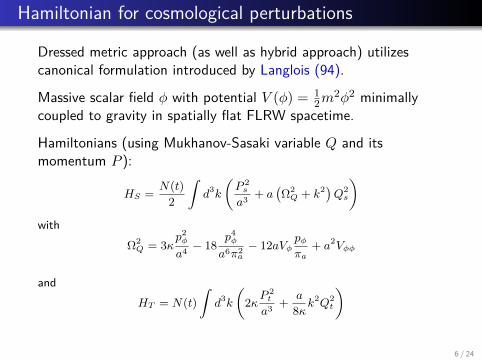
Dressed metric approach (as well as hybrid approach) utilizescanonical formulation introduced by Langlois (94).

Massive scalar field φ with potential V (φ) = 12m

2φ2 minimallycoupled to gravity in spatially flat FLRW spacetime.

Hamiltonians (using Mukhanov-Sasaki variable Q and itsmomentum P ):

HS = N(t)2

∫d3k

(P 2s

a3 + a(Ω2Q + k2)Q2

s

)with

Ω2Q = 3κ

p2φ

a4 − 18p4φ

a6π2a− 12aVφ

pφπa

+ a2Vφφ

andHT = N(t)

∫d3k

(2κP

2t

a3 + a

8κk2Q2

t

)

6 / 24

PerturbationsEquation of motion (scalar perturbations):

Qk + 3HQk + k2 + Ω2

a2 Qk = 0

with Ω2 determined from dressed metric approach.

Ω2 = 〈H−1/20 a2Ω2a2H

−1/20 〉

〈H−1/20 a4H

−1/20 〉

In the test-field approximation using sharply peaked states,background quantities in Mukhanov-Sasaki equation can bereplaced by their analogs in the effective spacetime description.

Primordial power spectrum computed at the end of inflation:

PR = k3

2π2|Qk|2

z2 , with z = φ/H

Similarly,

PT = 16k3

π|Qk|2

7 / 24

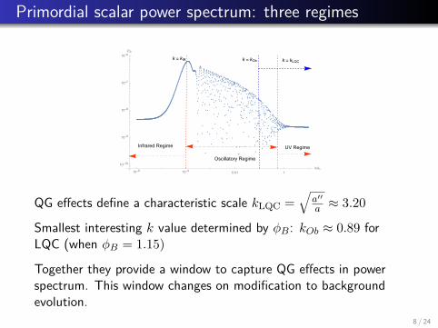
Primordial scalar power spectrum: three regimes

UV RegimeInfrared Regime

Oscillatory Regime

k = kLQCk = kIR k = kOb

10-6 10-4 0.01 1k/k*

10-10

10-9

10-8

10-7

10-6PS

QG effects define a characteristic scale kLQC =√

a′′

a ≈ 3.20

Smallest interesting k value determined by φB: kOb ≈ 0.89 forLQC (when φB = 1.15)

Together they provide a window to capture QG effects in powerspectrum. This window changes on modification to backgroundevolution.

8 / 24

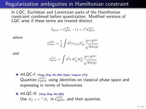
Regularization ambiguities in Hamiltonian constraintIn LQC, Euclidean and Lorentzian parts of the Hamiltonianconstraint combined before quantization. Modified versions ofLQC arise if these terms are treated distinct.

Cgrav = C(E)grav − (1 + γ2)C(L)

grav

whereC(E)

grav =12

∫d3x εijkF

iab

EajEbk√det(q)

andC(L)

grav =∫

d3xKj[aK

kb]EajEbk√

det(q)

mLQC-I: (Yang, Ding, Ma (09); Dapor, Liegener (17))

Quantize C(L)grav using identities on classical phase space and

expressing in terms of holonomies.

mLQC-II: (Yang, Ding, Ma (09))

Use Kia = γ−1Aia in C(L)

grav, and then quantize.9 / 24

Effective Hamiltonians for mLQC-I and mLQC-IImLQC-I:

HmLQC−I =3v

8πGλ2

sin2(λb)−

(γ2 + 1) sin2(2λb)4γ2

+HM , λ2 = 4

√3πγ`2Pl

Two branches for b. Switch from one to another at bounce.Bounce density ρI

c = ρc4(γ2+1) with ρc = 3

8πGλ2γ2

mLQC-II:HmLQC−II = −

3v2πGλ2γ2 sin2

(λb

2

)1 + γ2 sin2

(λb

2

)+HM

Bounce at ρIIc = 4(γ2 + 1)ρc

Comparison with LQC:

-20 -10 10 20t

100

104

106

108

1010

v

10 / 24

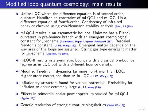
Modified loop quantum cosmology: main resultsUnlike LQC where the difference equation is of second order,quantum Hamiltonian constraint of mLQC-I and mLQC-II is adifference equation of fourth-order. Consistency of infra-redbehavior checked using von-Neumann stability analysis (Saini, PS (19))

mLQC-I results in an asymmetric bounce. Universe has a Planckcurvature in pre-bounce branch with an emergent cosmologicalconstant for µ-scheme (Assanioussi, Dapor, Liegener, Pawlowski (18)). RescaledNewton’s constant (Li, PS, Wang (18)). Emergent matter depends on theway area of the loops are assigned. String gas type emergent matterfor µ0-scheme (Liegener, PS (19)).mLQC-II results in a symmetric bounce with a classical pre-bounceregime as in LQC but with a different bounce density.Modified Friedmann dynamics far more non-trivial than LQC.Higher order corrections than ρ2 in LQC (Li, PS, Wang (18)).Inflationary attractors found for various potentials. Probability forinflation to occur extremely large (Li, PS, Wang (19)).Effects in primordial scalar power spectrum studied for mLQC-I(Agullo (18)).Generic resolution of strong curvature singularities (Saini, PS (18))

11 / 24

Initial conditions for different modelsIf initial conditions of the background are given at the bounce thenthe only free parameter is φB. For existence of a non-trivialwindow to capture QG effects, choose φB such that kLQC > kOb(similarly for mLQC-I and mLQC-II).

For all models, we require 72 e-folds during inflation. Thisdetermines φB in different models.

In LQC: φB = 1.15mPl (kLQC = 3.20; kOb ≈ 0.89)In mLQC-I φB = 1.27mPl (kmLQC−I = 1.60; kOb ≈ 0.65)In mLQC-II φB = 1.04mPl (kmLQC−II = 6.40; kOb ≈ 1.11)

Evolve universe backward from bounce at φB and specify initialconditions for perturbations as 4th-order adiabatic states att ≈ −1.1× 105 tPl for LQC and mLQC-II.

Pre-bounce regime in mLQC-I mimics deSitter evolution. ChooseBunch-Davies vacuum as initial state, as in (Agullo (18)).

12 / 24

Ambiguity in treatment of πa

Subtlety: Ω2Q contains inverse powers of πa.

Classically πa = −6aa/κN . If used in LQC it vanishes at bouncemaking Ω2

Q singular.

Strategy: (Agullo, Ashtekar, Nelson (13))

Vanishing of the background classical Hamiltonian constraint

H(0) = −κπ2a

12a +p2φ

2a3 + a3V ≈ 0

implies 1/π2a = κ/(12a4ρ). Leads to

Ω2+ = a2 (Vφφ + 2fVφ + f2V

), where f =

√24πG/ρφ

with a and ρ determined from effective dynamics.

Above expression true only for expanding branch where πa isnegative. (Zhu et al (18); Navascues, de Blas, Marugan (18))

Another strategy: Use solution of effective dynamics. Differencesappeared significant only in infra-red regime (Agullo, Bolliet, Sreenath(18))

13 / 24

In the contracting branch,

Ω2− = a2 (Vφφ − 2fVφ + f2V

)Discontinuity in Ω2

Q at the bounce.

Inspired by a strategy used in the hybrid approach, we can assumea smooth extension

Ω2 = a2(Vφφ + 2 cos (λb) fVφ + f2V

)

Ω+

Ω-

Ω

-0.6 -0.4 -0.2 0.0 0.2 0.4 0.6

1.×10-10

2.×10-10

3.×10-10

4.×10-10

5.×10-10

6.×10-10

t

14 / 24

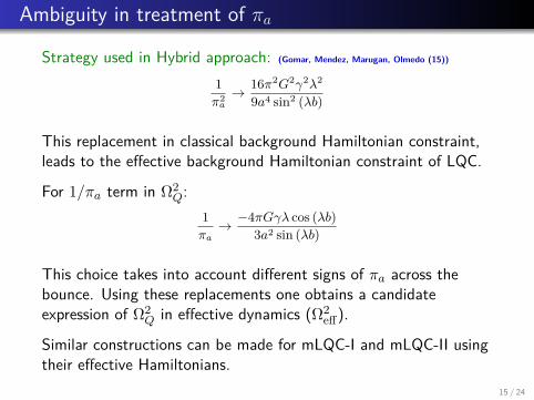
Ambiguity in treatment of πa

Strategy used in Hybrid approach: (Gomar, Mendez, Marugan, Olmedo (15))

1π2a→ 16π2G2γ2λ2

9a4 sin2 (λb)

This replacement in classical background Hamiltonian constraint,leads to the effective background Hamiltonian constraint of LQC.

For 1/πa term in Ω2Q:

1πa→ −4πGγλ cos (λb)

3a2 sin (λb)

This choice takes into account different signs of πa across thebounce. Using these replacements one obtains a candidateexpression of Ω2

Q in effective dynamics (Ω2eff).

Similar constructions can be made for mLQC-I and mLQC-II usingtheir effective Hamiltonians.

15 / 24

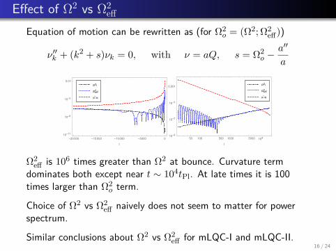
Effect of Ω2 vs Ω2eff

Equation of motion can be rewritten as (for Ω2o = (Ω2; Ω2

eff))

ν ′′k + (k2 + s)νk = 0, with ν = aQ, s = Ω2o −

a′′

a

|Ω|

|Ω |

| /|

-20000 -15000 -10000 -5000 010-11

10-8

10-5

0.01

t

|Ω|

|Ω |

| /|

50 100 500 1000 5000 10410-9

10-7

10-5

0.001

t

Ω2eff is 106 times greater than Ω2 at bounce. Curvature term

dominates both except near t ∼ 104tPl. At late times it is 100times larger than Ω2

o term.

Choice of Ω2 vs Ω2eff naively does not seem to matter for power

spectrum.

Similar conclusions about Ω2 vs Ω2eff for mLQC-I and mLQC-II.

16 / 24

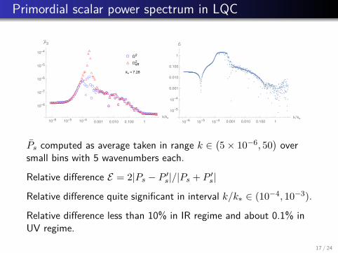
Primordial scalar power spectrum in LQC

Ω2

Ωeff2

k* = 7.28

10-6 10-5 10-4 0.001 0.010 0.100 1k/k*

10-8

10-7

10-6

10-5

10-4

PS

10-6

10-5

10-4

0.001 0.010 0.100 1

k /k*

10-5

10-4

0.001

0.010

0.100

1

ℰ

Ps computed as average taken in range k ∈(5× 10−6, 50

)over

small bins with 5 wavenumbers each.

Relative difference E = 2|Ps − P ′s|/|Ps + P ′s|

Relative difference quite significant in interval k/k∗ ∈ (10−4, 10−3).

Relative difference less than 10% in IR regime and about 0.1% inUV regime.

17 / 24

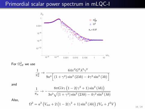
Primordial scalar power spectrum in mLQC-I

Ωeff2

Ω2

k* = 5.57

10-5 10-4 0.001 0.010 0.100 1 10k/k*

10-12

10-9

10-6

0.001

1

PS

For Ω2eff we use

1π2a→ 64π2G2λ2γ2

9a4[

(1 + γ2) sin2 (2λb)− 4γ2 sin2 (λb)]

and1πa→ −

8πGλγ(1− 2(γ2 + 1) sin2 (λb)

)3a2√

(1 + γ2) sin2 (2λb)− 4γ2 sin2 (λb)Also,

Ω2 = a2 (Vφφ + 2(1− 2(γ2 + 1) sin2 (λb)

)fVφ + f2V

)18 / 24

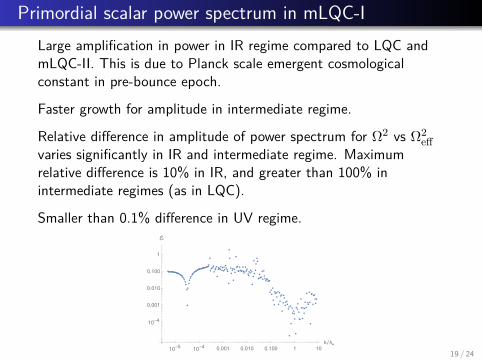
Primordial scalar power spectrum in mLQC-ILarge amplification in power in IR regime compared to LQC andmLQC-II. This is due to Planck scale emergent cosmologicalconstant in pre-bounce epoch.

Faster growth for amplitude in intermediate regime.

Relative difference in amplitude of power spectrum for Ω2 vs Ω2eff

varies significantly in IR and intermediate regime. Maximumrelative difference is 10% in IR, and greater than 100% inintermediate regimes (as in LQC).

Smaller than 0.1% difference in UV regime.

10-5

10-4

0.001 0.010 0.100 1 10

k /k*

10-4

0.001

0.010

0.100

1

ℰ

19 / 24

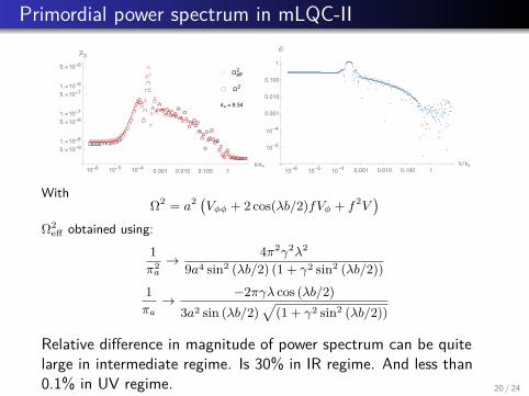
Primordial power spectrum in mLQC-II

Ωeff2

Ω2

k* = 9.54

10-6 10-5 10-4 0.001 0.010 0.100 1k/k*

5.×10-91.×10-8

5.×10-81.×10-7

5.×10-71.×10-6

5.×10-6

PS

10-6

10-5

10-4

0.001 0.010 0.100 1

k /k*

10-5

10-4

0.001

0.010

0.100

1

ℰ

WithΩ2 = a2 (Vφφ + 2 cos(λb/2)fVφ + f2V

)Ω2

eff obtained using:1π2a→ 4π2γ2λ2

9a4 sin2 (λb/2) (1 + γ2 sin2 (λb/2))

1πa→ −2πγλ cos (λb/2)

3a2 sin (λb/2)√

(1 + γ2 sin2 (λb/2))

Relative difference in magnitude of power spectrum can be quitelarge in intermediate regime. Is 30% in IR regime. And less than0.1% in UV regime. 20 / 24

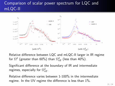
Comparison of scalar power spectrum for LQC andmLQC-II

mLQC-II

LQC

10-5 10-4 0.001 0.010 0.100 1 10k

5.×10-91.×10-8

5.×10-81.×10-7

5.×10-71.×10-6

PS

LQC

mLQC-II

10-5 10-4 0.001 0.010 0.100 1 10k

10-8

10-7

10-6

10-5

10-4

PS

(with Ω2) (with Ω2eff)

Relative difference between LQC and mLQC-II larger in IR regimefor Ω2 (greater than 60%) than Ω2

eff (less than 40%).

Significant difference at the boundary of IR and intermediateregimes, especially for Ω2

eff .

Relative difference varies between 1-100% in the intermediateregime. In the UV regime the difference is less than 1%.

21 / 24

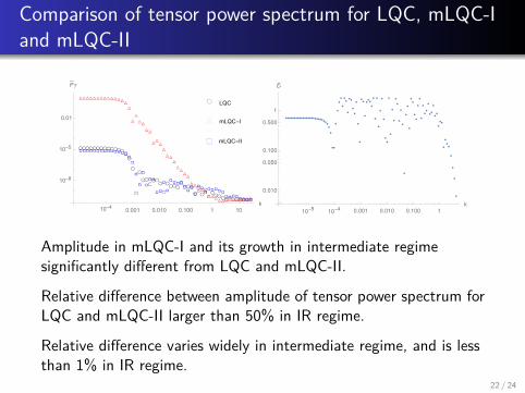
Comparison of tensor power spectrum for LQC, mLQC-Iand mLQC-II

LQC

mLQC-I

mLQC-II

10-4 0.001 0.010 0.100 1 10k

10-8

10-5

0.01

PT

10-5

10-4

0.001 0.010 0.100 1

k

0.010

0.050

0.100

0.500

1

ℰ

Amplitude in mLQC-I and its growth in intermediate regimesignificantly different from LQC and mLQC-II.

Relative difference between amplitude of tensor power spectrum forLQC and mLQC-II larger than 50% in IR regime.

Relative difference varies widely in intermediate regime, and is lessthan 1% in IR regime.

22 / 24

Summary and conclusions

Different treatments of the Lorentzian term in the Hamiltonianconstraint, result in non-trivial changes in physics of bounceand pre-bounce. Still, mLQC-II bears qualitative similaritywith LQC. However, mLQC-I results in an asymmetric bouncewith a pre-bounce universe with Planckian curvature.Treatment of πa in the scalar perturbation Hamiltonian hasbeen performed in different ways. We used approaches usedwidely in dressed metric as well as one inspired from hybridapproach.Results between LQC, mLQC-I and mLQC-II agree in UVregime (contributing most to observable modes) whereambiguity in πa is also of little significance.

Qualitative predictions for observable modes for linearperturbations in dressed metric approach robust to consideredHamiltonian regularization and πa ambiguities.

23 / 24

Summary and conclusions

However, these ambiguities do leave a significant trace in IRand intermediate regimes.Relative difference between LQC and mLQC-II can be as largeas 50-100% in IR and in intermediate regimes depending onchoice of πa.mLQC-I in IR and intermediate regime leaves qualitativelydifferent signatures with a very large amplitude and its rapidgrowth of amplitude for scalar as well as tensor powerspectrum.Different choices of πa generally result in at least 10% relativedifference in IR and intermediate regimes for the same model.

Do these differences due to ambiguities translate to qualitativelydifferent observable signatures, such as in non-gaussianities?

24 / 24