Effect of Adaptive Tabs on Drag of a Square-Base Bluff Body

EFFECT OF ADAPTIVE TABS ON DRAG OF A SQUARE-BASE BLUFF BODY

A Thesis

presented to

the Faculty of California Polytechnic State University,

San Luis Obispo

In Partial Fulfillment

of the Requirements for the Degree

Master of Science in Aerospace Engineering

by

Brian William Barker

August 2014

ii

© 2014


ALL RIGHTS RESERVED

iii

COMMITTEE MEMBERSHIP

TITLE:

AUTHOR:

DATE SUBMITTED:

COMMITTEE CHAIR:

COMMITTEE MEMBER:

COMMITTEE MEMBER:

COMMITTEE MEMBER:

Effect of Adaptive Tabs on Drag of a Square-

Base Bluff Body


August 2014

Jin Tso, Ph.D.

Professor of Aerospace Engineering

Dianne DeTurris, Ph.D.


Faysal Kolkailah, Ph.D.


Russell Westphal, Ph.D.

Professor of Mechanical Engineering

iv

ABSTRACT

Effect of Adaptive Tabs on Drag of a Square-Base Bluff Body


This thesis involves the experimental wind tunnel testing of a 0.127m by 0.127m

square-base bluff body to test the effectiveness of trailing edge tabulations to reduce drag

in the Cal Poly 0.912m by 1.219 m low-speed wind tunnel. To accomplish this, the

boundary layer was first measured on the trailing edge of the model for the three speeds

at 10, 20, and 30 m/s, with Re = 8.3e4, 1.6e5 and 2.5e5 respectively, without the tabs.

Three different tests were performed to determine the effectiveness of the tabs. These

tests included base pressure measurements, total drag force measurements and hotwire

velocity fluctuation measurements. These tests were repeated with tabs on the model’s

trailing edge at the three different tab heights and without tabs at all three test speeds.

The base pressure measurements showed a decrease in average base pressure with the

addition of tabs which signifies an increase in drag. The total drag measurements

confirmed this by showing that the overall force increases with the addition of the tabs.

The hotwire tests further confirm this by showing that the vortex is present for every

configuration tested.

This thesis showed that the addition of tabs was unsuccessful in reducing the effects of

the vortex shedding for a square-base bluff body. The addition of low, medium, and high

tabs to the square base of the bluff body all showed an increase in vortex strength and

overall drag. Further study is required to determine if drag savings are feasible for tabs all

around the square base of the bluff body and at different locations.

v

ACKNOWLEDGMENTS

Through this long process of designing, testing and defending I have many thanks to

give. First I would like to thank Dr. Tso for taking me on as a graduate student and

guiding me through the experiment. I would then like to thank Cody Thompson for his

help building the model and maintaining the wind tunnel. I would also like to thank my

amazing family and friends for all of their support and encouragement through this long

and difficult process.

vi

TABLE OF CONTENTS

Page

LIST OF TABLES ........................................................................................................... viii

LIST OF FIGURES ........................................................................................................... ix

CHAPTER

1. INTRODUCTION ....................................................................................................... 1

2. LITERATURE REVIEW ............................................................................................ 3

3. EXPERIMENTAL APPARATUS .............................................................................. 6

3.1 Experimental Model ..............................................................................................6

3.2 Wind Tunnel ........................................................................................................13

3.3 Scanivalve ...........................................................................................................15

3.4 Sting Balance.......................................................................................................18

3.5 Traverse System ..................................................................................................20

3.6 Boundary Layer Probe ........................................................................................21

3.7 Hotwire Probe .....................................................................................................22

4. PROCEDURES ......................................................................................................... 27

4.1 Wind Tunnel Calibration .....................................................................................27

4.2 Longitudinal Pressure Profile ..............................................................................28

4.3 Boundary Layer Velocity Profile ........................................................................29

4.4 Base Pressure.......................................................................................................30

4.5 Sting Balance.......................................................................................................30

4.6 Hotwire Velocity Spectra ....................................................................................31

5. ANALYSIS ............................................................................................................... 32

5.1 Reynolds Number ................................................................................................32

vii

5.2 Pressure Coefficient ............................................................................................32

5.3 Drag Coefficient ..................................................................................................33

5.4 Strouhal Number .................................................................................................33

6. RESULTS AND DISCUSSION ................................................................................ 34

6.1 Wind Tunnel Correlation Results ........................................................................34

6.2 Longitudinal Pressure Profile ..............................................................................35

6.3 Boundary Layer Velocity Profiles.......................................................................37

6.4 Base Pressure Coefficients ..................................................................................41

6.5 Sting Balance Drag Results .................................................................................53

6.6 Hotwire Energy Spectra ......................................................................................55

7. DISCUSSION ............................................................................................................ 61

8. CONCLUSIONS ....................................................................................................... 63

REFERENCES ................................................................................................................. 65

APPENDICES

A. Sample Error Calculations .........................................................................................66

B. Sample Pressure Code ...............................................................................................67

C. Sample Boundary Layer Code ...................................................................................69

viii

LIST OF TABLES

Table Page

1. Boundary Layer Results ........................................................................................ 38

2. Changes in average CPb Magnitude Compared to No Tab Configuration. ........... 47

3. Change in CD with Tabs Compared to No Tab Configuration. ............................ 55

ix

LIST OF FIGURES

Figure Page

Fig. 1. Experimental model mounted in wind tunnel.......................................................... 6

Fig. 2. Schematic of test model. .......................................................................................... 7

Fig. 3. Removable rear plates and rear plate on model in wind tunnel. .............................. 8

Fig. 4. Rear plate schematic. Tab heights are 0.0059 m, 0.0043 m, and 0.0038 m

(0.2338, 0.1687, and 0.1487 inches). ................................................................... 10

Fig. 5. Side and back plate pressure port distribution schematic. ..................................... 11

Fig. 6. Hollow strut mount attached to experimental model............................................. 13

Fig. 7. Cal Poly wind tunnel laboratory. On the left there is a removable test

section. Next to the removed section is the inlet followed by the attached test

section and then the exhaust nozzle. ..................................................................... 14

Fig. 8. Adapter plate (left), ZOC33 Scanivalve (right), and vacuum gun (top). ............... 16

Fig. 9. Model internal tubing on sting balance. ................................................................ 17

Fig. 10. Manometer used to calibrate the scanivalve. ....................................................... 17

Fig. 11. Sting balance calibration schematic. ................................................................... 19

Fig. 12. Sting balance controller. ...................................................................................... 19

Fig. 13. Traverse window. ................................................................................................ 20

Fig. 14. Traverse mounted to side of wind tunnel. ........................................................... 21

Fig. 15. Boundary layer probe at the trailing edge of the model. ..................................... 22

Fig. 16. IFA-300 hotwire anemometry cabinet. ................................................................ 23

Fig. 17. Hotwire probe behind model. .............................................................................. 24

Fig. 18. Hotwire probe and probe support. ....................................................................... 25

Fig. 19. Manual hotwire velocity calibrator...................................................................... 26

x

Fig. 20. Wind tunnel Variable Frequency Drive controller (right) and dynamic

pressure anemometer (left). .................................................................................. 28

Fig. 21. Wind tunnel calibration results. ........................................................................... 35

Fig. 22. This experiment’s pressure coefficient profile results. ........................................ 36

Fig. 23. Knight and Tso’s pressure profile results [4]. ..................................................... 37

Fig. 24. Boundary layer velocity profile for 10 m/s test. .................................................. 39

Fig. 25. Boundary layer velocity profile for 20 m/s test. .................................................. 40

Fig. 26. Boundary Layer velocity profile for 30 m/s testing. ........................................... 41

Fig. 27. Park et al. data [3]. Solid square was optimally controlled flow with a

pair of tabs. Solid circle data was uncontrolled flow. Open circle data was

Bearman’s uncontrolled flow. Solid triangle data was a two dimensional

fence of tabs. ......................................................................................................... 43

Fig. 28. Base pressure results for 10 m/s tests. ................................................................. 44

Fig. 29. Base Pressure results for 20 m/s tests. ................................................................. 45

Fig. 30. Base pressure profiles for 30 m/s tests. ............................................................... 46

Fig. 31. Normal base CPb distribution for each tab height with varying speeds. .............. 48

Fig. 32. Spanwise base pressure results for 10 m/s tests. ................................................. 49



Fig. 35. Spanwise base Cpb distribution for each tab height with varying speeds. ........... 52

Fig. 36. Sting balance calibration curve............................................................................ 53

Fig. 37. Coefficient of drag results for all four tab configurations at all three

speeds. ................................................................................................................... 54

xi

Fig. 38. Calibration curve for the hotwire probe. ............................................................. 56

Fig. 39. Energy spectra results for 10 m/s speed for all four tab configurations. ............. 57



Fig. 42. Comparison of model aspect ratios. .................................................................... 62

Fig. 43. Schematic of vortices........................................................................................... 62

xii

NOMENCLATURE

Greek

δ

εsb

ρ

θ

λ

Alpha Numeric

2D

3D

CD

CP

CPb

f

FFT

h

Kε

ly

lz

ptot

p∞

q∞

Re

St

U∞

V

Boundary layer height

Solid blockage coefficient

Density

Momentum thickness

Spacing between tabs

Two dimensional

Three dimensional

Coefficient of drag ,

.

Coefficient of pressure ,

.

Base coefficient of pressure,

Frequency

Fast Fourier transform

Height of the model

Blockage coefficient

Height of tabs

Width of tabs

Total pressure

Free stream pressure

Free stream dynamic pressure

Reynolds number,

Strouhal number,

Free stream velocity

Voltage

xiii

u,v,w

x,y,z

Superscripts and

Subscripts

D

P

Pb

tot

u,v,w

x,y,z

∞

Streamwise, normal and spanwise velocity

Streamwise, normal and spanwise coordinates

Drag

Pressure

Base pressure

Total (pressure)

Streamwise, normal and spanwise velocity

Streamwise, normal and spanwise coordinates

Free stream

1

1. INTRODUCTION

The focus of this thesis is to find a passive way to reduce drag on a bluff body. A bluff

body is any body whose dominant source of drag is pressure drag. For all of the work

done in this thesis and the work done previously [1-2], the bluff body consisted of a

rectangular cross section with a blunt trailing edge and either an elliptical or a circular

leading edge.

Engineers are always looking for ways to reduce drag on aerodynamic systems. This

includes more than just aircraft. One main reason for drag reduction on a vehicle is to

improve fuel efficiency and reduce operational costs. This goal relates to this experiment

because most cargo transport vehicles closely resemble a bluff body with a fairly

aerodynamic leading edge and a relatively blunt trailing edge. Currently there are

methods in use to reduce drag such as the tapered extensions on the back of large semi-

trailers. The goal of this experiment is to improve upon these methods.

A bluff body poses many interesting aerodynamic problems because of its geometry.

Due to its many uses a bluff body is still a necessity for many modern designs. The

circular or elliptic leading edge can be considered to have good aerodynamic properties,

but the blunt trailing edge is the prominent source of pressure drag. This large source of

drag is caused by flow separation and is further increased by a phenomenon called Von

Kármán Vortex Shedding. Kármán Vortex Shedding is caused by the sudden separation

of the flow around the body. Because of the ninety degree turn at the trailing edge, the

flow instantaneously separates, forming the shear layer, and then subsequently rolls-up

into vortices behind the body. The vortices from the four sharp edges are what create an

2

increase in suction behind the body, increasing the drag. By attenuating the vortices the

drag can be reduced.

Similar experiments deal with distributed forcing of the trailing edge of the body.

Distributed forcing is a type of active flow control that uses the blowing or suction of air

into the flow at the trailing edge to control vortex shedding. Distributed forcing in the

trailing edge has proven to reduce drag on many types of bodies, but thus far has not

proven completely successful on a bluff body.

This thesis will look into ways of reducing the drag caused by a bluff body through

wind tunnel testing and the addition of passive tabs on the model’s trailing edge. These

tests include surface pressure measurements, total drag measurements via a sting balance,

boundary layer measurements, and hotwire velocity fluctuation measurements.

3

2. LITERATURE REVIEW

The beginning of this series of experiments started at Cambridge University by an

engineer named Bearman [1-2]. Bearman did two experiments to reduce bluff body drag,

the first used splitter plates [1] and the second used base bleed [2]. In Bearman’s first

experiment, a splitter plate was connected to the trailing edge of the model and ran

parallel to the flow. The plate spanned the entire width of the model and essentially

separated the wake from the top and bottom surfaces of the model. Bearman’s results

showed that the addition of the splitter plate was sufficient to increase the base pressure

coefficient of the model. This confirms the theory that removing, or prolonging, the

vortex shedding was a feasible way to reduce the overall drag. In Bearman’s second

experiment [2] he was able to reduce the vortex shedding at high speeds over a bluff body

by having compressed air escape from the base of the model.

These experiments were then continued by a group of Korean engineers led by

Hyungmin Park et al. [3] who did wind tunnel testing on a two dimensional bluff body.

This model was two dimensional because it spanned the entire width of the wind tunnel.

Their results showed that the drag could be reduced by using passive trailing edge tabs at

all three of the test speeds. They also did large eddy simulations on the computer to

validate their theory for the mechanism of drag reduction.

Using the large eddy simulations, Park et al. [3] were able to show that the increase in

the wake width was the main method for reducing vortex strength. Without tabs the wake

was the same width along the entire model. By adding the tabs it created an area of

thicker wake width behind the tabs. The change in wake width across the span of the

trailing edge created a mixing factor within the wake. This mixing prolonged the

4

formation of the vortex, increased the formation length, and reduced its effect on the

body. The increase in wake width decreased the interaction between the top and bottom

vortices and caused an increase in base pressure, thus reducing drag. These results are

shown visually in Park’s paper.

At the same time, the first bluff body experiment was being conducted at Cal Poly by

James Knight and Jin Tso [4-5]. This experiment focused on drag reduction on a bluff

body by use of passive surface roughness at the leading edge. Knight’s research also

measured the trailing edge boundary layer response due to the various roughness of trip

tape at the leading edge. In his research Knight was able to show that with increasing

surface roughness, the base pressure was increased which decreased the base drag. This

however did not hold true at higher Reynolds numbers.

To expand upon Park’s two dimensional results, a former Cal Poly student, Jarred

Pinn [6], created a three dimensional model to test. Pinn had a cylindrical leading edge

with a 4 to 1 cross sectional aspect ratio. His tests proved that even in three dimensions

the passive tabs led to a significant reduction in drag but only for the two lower speed

cases. The high speed test showed that the tabs actually increased the overall drag of the

body. Because of this increase in drag, it is believed that the original equations used by

Park to determine the tab height are invalid at high speeds for a 3D model. Instead it is

now believed that the tab height is more dependent on the thickness of the boundary layer

instead of just the model width. Two other Cal Poly students, Paul Innes and Charles

Carlson [7], did a senior project to validate Pinn’s base pressure results. While they were

not able to reproduce the same curves they were able to come to the same conclusion:

that the tabs do increase the average base pressure.

5

Another former student, Ethan Erlhoff [8], tested the distributed forcing in the trailing

edge of a bluff body. For his model Ethan used a high aspect ratio 3D body with an

elliptical leading edge with a blunt trailing edge. This model had four slots in the top and

bottom of the trailing edge that were then connected by internal ducts to an electric fan

that would control the blowing or suction through the slots.

Erlhoff’s results did show significant reductions in drag, but still needed energy input

to operate the fans. For the lower test speeds this was not a problem because the energy

saved by the drag reduction was greater than the electrical energy that was added.

Unfortunately, to get drag savings at higher speeds the electrical energy input to the

system far outweighed the drag savings. These results showed that active flow control for

a bluff body was plausible but with the current technology it does not outweigh the

energy costs.

Because of the success of Pinn’s study on the effectiveness of end plate tabs in

attenuating vortices and reducing drag at lower Reynolds numbers, this thesis looked into

ways of reducing the drag caused by a bluff body with square base with the addition of

passive tabs on the model’s trailing edge.

6

3. EXPERIMENTAL APPARATUS

This section describes the design and implementation of the experimental model as

well as the testing equipment. It is also discussed how the testing equipment was

calibrated and configured. Calibration results are discussed in the results and discussion

section.

3.1 Experimental Model

Fig. 1. Experimental model mounted in wind tunnel.

The model that was used for this experiment is very similar to previous experiments

[3,4] and can be seen mounted in the wind tunnel above in Fig. 1 . Each of the previous

models was slightly different and this model is the next step in the progression to prove

the usefulness of the passive tabs. The Park et al. model [3] was two dimensional, both

Pinn’s model [6] and Knight’s model [4-5] were three dimensional, but still had high

aspect ratios. The current model is similar in construction to Pinn’s in that they were both

7

made out of 6061 aluminum with a circular nose, but this model has a cross sectional

aspect ratio of 1 to 1. A schematic of the model can be seen below in Fig. 2. As shown it

has a cross section with a height and width of 0.127 m (5 inches). The leading edge of the

model is composed of a half cylinder with a radius of 0.0635 m (2.5 inches). The length

of the entire model was chosen to be similar to that of Pinn’s experiment and overall is

0.2984 m (11.75 inches) long.

Fig. 2. Schematic of test model.

Along with a different aspect ratio, this model improves upon previous tab designs.

The previous two experiments [3,6] had "static" tabs that were dependent only on the

width of the model. Because of Pinn’s results at high speeds [6], this model was designed

with "adaptive" tabs. This means that instead of the tab height being dependent on the

width of the model; it will now change depending on the momentum thickness. As

8

discussed later, the tabs are designed to protrude into the flow less as the speed increases.

This adaptive tab height can be seen in the schematic in Fig. 4 below. Based on tests

discussed later in this paper, the tabs were set to protrude 0.0059 m, 0.0043 m, and

0.0038 m (0.2338, 0.1687, and 0.1487 inches) into the flow for speeds of 10, 20, and 30

m/s (32.8, 65.6, and 98.4 ft/s) respectively. These will be referenced later as high,

medium, and low tabs for the 10, 20, and 30 m/s speeds respectively.

Fig. 3. Removable rear plates and rear plate on model in wind tunnel.

As shown in Fig. 3 the tabs are built into three removable rear plates that screw into

the trailing edge of the model. These removable plates allow for the tab heights to be

9

easily reconfigured. Using removable tabbed plates, the rear plate of the model does not

need to be opened and the tubing does not need to be reconfigured as in previous

experiments. This improvement allows for quicker and easier setup changes as well as

more consistent data while reducing the probability of tubing leaks. In the tab schematic

in Fig. 4 below, it shows three different numbers on the tabs. These are the tab heights for

each test, not for each tab. For all three test configurations, all six tabs were the same

height. The tab spacing was determined by keeping the tabs as similar as possible to

previous experiments. In both Park et al. and Pinn’s experiment the tabs were sized based

on a ratio of base area to tab area. Because this model has a similar area to Pinn’s the

width of each tab was set equal to Pinn’s tab width. The tab spacing was then determined

based on having an already set tab width and then equally spacing the three tabs across

the body.

10

Fig. 4. Rear plate schematic. Tab heights are 0.0059 m, 0.0043 m, and 0.0038 m (0.2338,

0.1687, and 0.1487 inches).

Fitted inside the model are sixty 0.0016 m (1/16th

inch) stainless steel pressure ports

with 0.0024 m (3/32nd

inch) Tygon PVC tubing that runs through the sting balance mount

and into a pressure transducer. This data is then sent to the computer for analysis. The

pressure port distribution can be seen in Fig. 5. Previous models had the pressure ports

run all the way around the nose but only one side is necessary to show the profile around

the body. The inner diameter of the Tygon tubing is smaller than the outer diameter of the

pressure ports and aluminum tubing to create an interference fit. This was done for ease

11

of setup and to reduce the risk of leaks, whereas in previous experiments lock wire was

required to connect the tubing to the ports [6].

Fig. 5. Side and back plate pressure port distribution schematic.

The ports were spaced in a way that maximizes the amount of relevant data. This is

done by putting more pressure ports near the edges of the model and fewer in the middle.

Towards the edges there is a 0.0032 m (1/8th

inch) spacing between each port and

towards the center there is a 0.0127 m (½ inch) spacing between ports. This allows for a

more accurate view of the influence of the vortex shedding on the pressure distribution.

12

To ensure that the influence of the vortex shedding on the pressure was captured in its

entirety, there are three rows of pressure ports on the base of the model. There are two

rows that run perpendicularly to the tabs along the normal direction. This is to allow the

measurement of the vortex over the tabs and between the tabs. The third row that runs

parallel to the tabs in the spanwise direction is to measure the vortex shedding from the

sides without tabs.

The model is mounted to the wind tunnel via a custom strut shown in Fig. 6. This strut

was made out of a hollow 4130 steel tube that was formed as a symmetric airfoil to

maintain smooth flow. At the top of the strut, as shown below, there is a plate with four

screws that screw directly into the test model. The bottom has two hollow cylinders

welded together. The bottom cylinder is where the strut mounts to the sting balance in the

wind tunnel. The top cylinder is to guide the internal tubing. As shown in Fig. 6 there are

thirty aluminum tubes that run through the airfoil section of the strut. These tubes are

used to connect the pressure ports inside the model to the scanivalve outside of the wind

tunnel. The width of the airfoil section limited the number of pressure tubes to thirty.

This space constraint is what limited the amount of pressure ports per row to fifteen. With

fifteen pressure ports per row, two rows can be tested simultaneously.

13

Fig. 6. Hollow strut mount attached to experimental model.

3.2 Wind Tunnel

All of the tests for this experiment were done in Cal Poly’s subsonic wind tunnel. This

tunnel is an open circuit wind tunnel that consists of a 3.66 meter by 2.74 meter (12 feet

by 9 feet) inlet with a 1.22 meter by 0.91 meter (4 feet by 3feet) test section. Built into

the floor of the test section is a sting balance built by Aerolab that is used to record the

forces on the model. The flow is kept laminar by placing the fan behind the test section

and pulling the air through the test section. This fan is a nine blade fixed pitch fan that is

driven by a 150 horsepower electric motor that is controlled by a SquareD Altivar66

manual variable frequency generator. The wind tunnel is in an enclosed room, but the

door behind the wind tunnel opens so the air can be expelled out of the room. There is

another vent in the ceiling by the inlet which brings in air from the outside. The tunnel

was constructed in 1974 by Professor Jon Hoffman with help from other faculty and

students. The tunnel was built primarily out of wood and has removable test sections to

allow for many different types of experiments. One of these removable sections can be

seen on the left of Fig. 7.

14

Fig. 7. Cal Poly wind tunnel laboratory. On the left there is a removable test section. Next

to the removed section is the inlet followed by the attached test section and then the

exhaust nozzle.

During testing the VFD (Variable Frequency Drive) for the tunnel broke down and the

tests had to be completed with two different motors. The first motor was an Elliott Co.

150 hp three phase electric motor and was used to complete the boundary layer testing as

well as the tunnel calibration and longitudinal pressure profile tests. The tunnel

calibration test was required because the velocity measurements used to control the

tunnel were for the inlet not the test section.

The second motor was an 125 hp three phase electric motor controlled by a Allen-

Bradley VFD and was used to complete the base pressure, total drag, and hotwire tests.

15

Instead of doing a tunnel calibration for these tests, a Pitot-static probe was inserted into

the tunnel in front of the model to measure the flow velocity in the test section. The probe

was placed in a mid-span location about 5h ahead of the model and 3h below the model,

outside the boundary layer on the wind tunnel wall. No other major changes were made

to the tunnel during the course of this experiment other than changing motors and

controllers.

3.3 Scanivalve

To measure the pressure along the top plate and base of the model, tubes were run

from the pressure ports along the model to the scanivalve outside the wind tunnel. The

scanivalve itself was a ZOC33/64P-X1 pressure scanner. It has the ability to read 64

pressure ports simultaneously with the added input of 448 kPa (65 psi) shop air as a

reference pressure. The first 32 ports have an input range of ±10 inches of water (2.491

kPad, 0.3613 psid) with an accuracy of ±0.15% full scale reading while the remaining 32

ports have an input of ±6.895 kPad (1 psid) and an accuracy of ±0.12% full scale reading.

The scanivalve can be seen in the center of Fig. 8 along with the adapter plate and

vacuum gun.

16

Fig. 8. Adapter plate (left), ZOC33 Scanivalve (right), and vacuum gun (top).

To make testing easier, an adapter plate was implemented between the model’s tubing

and the scanivalve to adapt the size of the tubing. This allows for the ports connected the

scanivalve to remain untouched and allow for more standardized tubing sizes to be used

on the experimental models.

Tubing was run from the ports along the model, through the hollow airfoil strut, out of

the wind tunnel and into the adapter plate. From there, smaller tubing was run into the

ZOC33 where the pressures were converted into voltages. These voltage values were then

sent to and amplified in a RAD3200 analog to digital converter. This data was then sent

to a computer running the RadLink V2.10 software that read and stored the data from the

pressure tests. The raw data was then processed using MATLAB. The internal tubing can

be seen in Fig. 9.

17

Fig. 9. Model internal tubing on sting balance.

The scanivalve was calibrated using a U-shaped manometer filled with water shown in

Fig. 10. A constant pressure was applied to the manometer and the computer tested each

port to make sure it was reading accurately.

Fig. 10. Manometer used to calibrate the scanivalve.

18

Between each test the model was checked for leaks. Though it was unlikely the tubes

came loose between tests, as they are not exposed to the flow, leak checking was done to

ensure accurate data. Leaks were checked by unplugging the tubing from the adapter

plate and connecting it to a vacuum gun. The pressure port on the model was then

covered by a finger and a pressure was applied via the vacuum gun. If the pressure stayed

constant then there were no leaks. If the pressure returned to zero then that tube was

checked immediately for the source of the leak.

3.4 Sting Balance

The model was held in place using a sting balance that was built into the floor of the

wind tunnel. This sting balance has the ability to not only move vertically in the tunnel

but also change the angle of attack and yaw angle of the test model. This is done

manually via the controller outside the wind tunnel or from the computer using LabView.

The controller can be seen in Fig. 12 below. For these tests the angle of attack and yaw

angle were always set to zero relative to the flow. Also built into the sting balance are

sensitive strain gauges that allow for the measurement of all six degrees of freedom. For

this experiment the axial force was measured to calculate the total coefficient of drag.

The sting balance sent a voltage from each of the six internal strain sensors through an

amplifier inside the controller and was then read by a data acquisition card. The data was

then sent to the computer and recorded using a custom LabView program. The sting

balance also acts as the mount that holds the test model in place. This was achieved via a

long tapered rod with a threaded hole at the end. The model mount slid over the tapered

rod and was pulled tight using a screw in a threaded hole causing a friction fit on the

tapered rod.

19

To calibrate the sting balance, small weights were used that ranged from 0.4536 to

2.268 kg (1 to 5 pounds) in increments of 0.4536 kg (one pound). The weights were hung

off of the tip of the sting balance and over a pulley to calibrate the axial force on the

sting. The voltage for each weight was recorded. The calibration setup can be seen in Fig.

11. The calibration produced a linear correlation between the weights and a trend line

was calculated. The equation of the trend line was later used to find the forces on the test

model.

Fig. 11. Sting balance calibration schematic.

Fig. 12. Sting balance controller.

20

3.5 Traverse System

Due to the need for high precision measurements inside the wind tunnel, the Velmex

Traverse system shown in Fig. 13 was used to move the hotwire and boundary layer

probes laterally through the tunnel. The Velmex traverse uses an electric stepper motor

and screw to slowly move a cart linearly. A metal plate was then attached to the cart on

the metal screw that extended into the wind tunnel. The traverse was then mounted to a

custom removable window that clamps into a slot on the side of the wind tunnel. The

traverse window can be seen mounted to the tunnel in Fig. 14. The window only sealed

on the top and bottom edges so aluminum tape was used to seal the remaining two sides

from the inside. A second aluminum arm was screwed to the metal plate on the traverse

to move the hotwire probe and boundary layer probe forward in the tunnel. The screw on

the traverse system was set up with a correlation of 4000 steps from the motor to rotate

the screw ten times and move the cart forward 0.0254 m (one inch). This was measured

and calibrated using a caliper prior to testing.

Fig. 13. Traverse window.

21

Fig. 14. Traverse mounted to side of wind tunnel.

3.6 Boundary Layer Probe

The boundary layer probe is a very small total pressure probe that was used in

conjunction with the traverse described above and a static port (port 15 in Fig. 5) on the

rear edge of the test model. The probe was a United Sensor Model BA-025-12-C-11-650

probe which has a sensing head diameter of 0.0006 m (0.025 inches), with a flattened

measuring orifice of 0.00028 m (0.011 inches) to minimize errors in total pressure

measurements. This probe can be seen next to the model in Fig. 15. The boundary layer

probe was used to measure the total pressure at incremental points away from the model.

The pressure was measured at small increments until the probe was far enough away

from the model to match the free stream total pressure.

22

Fig. 15. Boundary layer probe at the trailing edge of the model.

3.7 Hotwire Probe

A hotwire probe and anemometry system was used to measure the fluctuations in the

near wake behind the model. This system measured voltages from the probe and

ThermalPro was used to analyze the data and produce an energy spectrum. This energy

spectrum was then compared to the Strouhal number to visually show a large spike in the

energy spectrum to signify the shedding of a vortex. The primary controller for the

hotwire was the TSI IFA-300 constant temperature anemometer shown in Fig. 16. It

supports a frequency response of 250 kHz or greater and allows for one or two channel

wire systems. For this experiment only a one wire probe was used.

To position the hotwire probe in the correct place behind the model, a second traverse

system was used. This setup is similar to the boundary layer probe setup in Fig. 15. The

initial setup for the hotwire used a different window and a different arm than in the

23

boundary layer tests shown in Fig. 17. This window allowed for vertical movement of the

arm as well as lateral movement within the tunnel. These two degrees of freedom allowed

the probe to be positioned anywhere in the tunnel’s cross section 0.1778 m (7 inches)

behind the model. As the testing progressed it was determined that the probe could not

move close enough to the model to show the vortex shedding. To fix this the traverse

from the boundary layer testing was used in conjunction with the new arm to move the

probe up to 0.0254 m (1 inch) behind the model.

Fig. 16. IFA-300 hotwire anemometry cabinet.

24

Fig. 17. Hotwire probe behind model.

The probe that was used in this experiment was a TSI model 1247A-T1.5 as seen in

Fig. 18. This probe was a two-channel probe but one wire was broken making it a one-

channel probe. This probe only had a working channel two wire, which had a

recommended operating resistance of 12.12 Ω and an operating temperature of 250˚C.

25

Fig. 18. Hotwire probe and probe support.

The hotwire was calibrated using the TSI model 1128A manual velocity calibrator in

Fig. 19 along with a 0 to 10 mmHg pressure transducer in Fig. 16 and the calibration

manual [9]. The calibrator has a rotating probe mount. In this experiment the probe

support was positioned to be directly above and parallel to the calibration flow source.

The 448 kPa (65psi) compressed air in the lab was run through a pressure regulator that

limits the pressure between 137.89 kPa (20psi) and 206.84 kPa (30psi). This was then

connected to the bottom of the calibrator. Coarse and fine adjustment knobs were used to

accurately control the flow velocity coming out of the calibrator. The pressure of the flow

was then sent to the pressure transducer and compared to the ambient pressure. This

pressure difference and the voltage read from the hotwire probe were sent into the

computer and analyzed with ThermalPro to create a relationship between voltage and

velocity.

26

Fig. 19. Manual hotwire velocity calibrator.

27

4. PROCEDURES

This section goes into the details for the procedure for each test. These tests include

wind tunnel calibration, longitudinal pressure profile, boundary layer profile, base

pressure, drag force, and hotwire velocity fluctuations.

4.1 Wind Tunnel Calibration

To calibrate the wind tunnel, a curve comparing the frequency of the motor to the

velocity of the wind tunnel was created. This linear curve can be seen in the results

section. To construct this curve, the dynamic pressure was measured at various wind

tunnel VFD frequencies. The wind tunnel VFD controller in Fig. 20 was able to accept

manual frequency inputs and hold them to ± 1Hz. The dynamic pressure of the tunnel and

hence the wind tunnel velocity was measured using the static rings built into the inlet of

the wind tunnel. The free stream dynamic pressure of the model was determined by a

local Pitot-static tube. A correction factor was then calculated between the dynamic

pressure at the inlet and the dynamic pressure at the test section. Using this correction

factor and the known VFD frequencies for inlet dynamic pressure, an equation was

created comparing the velocity in the test section to the VFD frequency.

28

Fig. 20. Wind tunnel Variable Frequency Drive controller (right) and dynamic pressure

anemometer (left).

4.2 Longitudinal Pressure Profile

Before any experimental testing could begin, the pressure profile from the nose of the

model to the trailing edge of the model analyzed to ensure the profile matched previous

work and to show that the model was aligned in the flow.

This test was conducted separately from the rear plate testing because only 30 pressure

ports could be tested at a time due to the limited number of aluminum tubes which could

pass through the strut. The wind tunnel was then run at all three speeds and data was

taken for pressure ports 1 through 30. The first 15 ports were along the centerline of the

model that start at the leading edge and continue to the trailing edge with the last 15 ports

representing the base region. There were also two data points taken for the free stream

29

static pressure and total pressure that were taken from the Pitot-static probe in the test

section. The data was recorded via RadLink and then processed with Matlab. A separate

data file was created for each speed and each tab configuration. The most important

profile test was the non-tabbed configuration because it shows the continuity of the flow

over the model. The pressure profile was measured for the other three configurations to

show changes in the base region.

4.3 Boundary Layer Velocity Profile

To measure the boundary layer, the probe was first put directly against the trailing

edge of the model. A data point was then taken and the boundary layer probe was moved

further away from the model incrementally taking new data points until the measured

total pressure matched the free stream total pressure. Each time the pressure was

measured with the boundary layer probe, the pressure was also measured in the model’s

static port to calculate the velocity. Due to stepping motor problems the screw on the

traverse was turned manually to move the pressure probe. Each data point in the

boundary layer was taken at an additional 1/8th

turn of the screw which correlates to

0.0003 m (1/80th

of an inch) away from the previous point. The dynamic pressure at each

point was then converted to a velocity using the total pressure from the boundary layer

probe and the pressure from the static port on the model. The velocity profile was then

analyzed using Matlab and the momentum thickness was calculated. The momentum

thickness was then compared with previous experiments to calculate the optimal tab

heights for each speed.

30

4.4 Base Pressure

The base pressure was measured for all three speeds in each of the no tab and three

tabbed configurations. This resulted in a total of twelve different test cases. Due to the

lack of space in the strut mount, only thirty ports could be tested at a time. For the first

round of testing the normal row of ports behind the tabs was tested along with the

spanwise ports. The second round of testing measured the normal row behind the tabs as

well as the normal row between the tabs. Each tab configuration was tested at all three

speeds, creating a data file for each speed. After all three speeds were tested the tab

configuration was changed and the three speeds were tested again. Changing the tab

configuration was done without opening the model via swapping the removable back

plates. When the model was mounted in the wind tunnel, the normal row was oriented

horizontally with respect to the wind tunnel and the spanwise row was oriented vertically

with respect to the tunnel. In this orientation the tabs are on the left and right sides of the

model. The pressure data was read from each data file and converted to CPb data and

analyzed in Matlab.

4.5 Sting Balance

The sting balance data was taken using LabView and processed using Excel and

Matlab. Before the testing began, the sting balance was calibrated using the correlation

between the measured voltage in the strain gage and the known calibration weights. A

baseline was then taken with the model mounted to the sting balance without any flow.

This allowed the model weight to be removed from the equation and only the effects of

the flow on the model were shown in the results. To this same end, the tunnel was run at

all three test speeds with only the strut mounted to the sting so its effects could also be

31

removed from the results. Total force measurements were then taken at all three speeds

for all four tab configurations. The force on the body was then calculated by subtracting

the force caused by the weight of the model as well as the force caused by the strut mount

from the total force measurements. Next the Coefficient of Drag was calculated using

Equ. (3).

4.6 Hotwire Velocity Spectra

After the hotwire was successfully calibrated the hotwire probe and probe support

were removed from the calibrator. The probe was then removed from the probe support

for safe keeping. Next, the probe support was installed on the end of the traverse and

moved into position 0.0254 m (1 inch) from the trailing edge of the model. The probe

was aligned parallel with one side of the model directly behind the center tab. The

hotwire probe was then reinserted into the probe support. Spectral density data was then

taken using ThermalPro for all three test speeds and all four tab configurations. For all

four tests and all three speeds the data was taken at 1kHz with a sample size of 16kpts.

This results in a frequency resolution of 0.977 Hz. Between each test configuration the

probe was removed while the tabbed plates were swapped to ensure the wire stayed

intact. The spectral density data was then processed in Matlab to calculate the energy

spectrum and Strouhal numbers. Calibration of the hotwire is discussed in more detail in

the results section.

32

5. ANALYSIS

This section is meant as a brief reference describing the major coefficients and non-

dimensional numbers in this paper and how they are calculated.

5.1 Reynolds Number

The Reynolds number is a dimensionless number that gives a ratio of inertial forces to

viscous forces. Normally the Reynolds number is calculated based on the length of the

model but in this experiment the Reynolds number is calculated based on model height to

stay consistent with previous experiments.

(1)

Where h is the height of the model, u∞ is the free stream velocity, and v is the

kinematic viscosity. This equation gives Reynolds numbers of 8.3e4, 1.6e5 and 2.5e5 for

the test speeds of 10 m/s, 20 m/s, and 30 m/s respectively. A standard kinematic viscosity

of 1.52e-5 m2/s was used as the standard is close to the experimental conditions in San

Luis Obispo.

5.2 Pressure Coefficient

The pressure coefficient is a dimensionless number that compares the pressures

throughout the flow field. In this experiment the pressure coefficient is calculated along

the longitudinal profile of the body and the base region to show the pressure distribution

around the body. The pressure coefficient is calculated by:

(2)

Where P is the pressure measured at each static port on the model, q∞ is the free

stream dynamic pressure which is calculated from the free stream static pressure, P∞, and

33

the free stream total pressure, PT. An example of the propagation of error in the pressure

coefficient can be seen in Appendix A.

5.3 Drag Coefficient

The drag coefficient is a non-dimensional quantity that is used to compare the drag

forces across different speeds of the experiment. The drag coefficient is calculated by:

(3)

where D is the drag force on the body, q∞ is the free stream dynamic pressure, and S is

the cross sectional area of the body (h * h). An example of the propagation of error in the

drag coefficient can be seen in Appendix A.

5.4 Strouhal Number

The Strouhal number is a ratio that describes the oscillations in a flow. This number is

useful in hotwire testing because it allows for comparison of frequencies between tests

with inputs of only model height and free stream velocity. This is calculated using this

equation:

(4)

where f is the vortex shedding frequency, h is the model height, and u∞ is the free stream

velocity.

34

6. RESULTS AND DISCUSSION

Here the results are shown and analyzed for each of the five tests performed. The

discussion in this section is meant to interpret the results individually and the reasoning

for why the results came out this way will be looked at in the following discussion

section.

6.1 Wind Tunnel Correlation Results

To create the wind tunnel correlation trend seen in the typical example of Fig. 21, the

frequency was set at increments of 5 Hz from 10 Hz to 40Hz and a final point was added

for 0 Hz. For this example the dynamic pressure was measured using a Pitot-static probe

in the tunnel test section without the model present. The average temperature in San Luis

Obispo during testing was 21o C (70

o F) so a standard density of 1.292 km/m

3 (1.225

slugs/ft3) and Equ. (5) below, the calibration curve shown in Fig. 21.

35

Fig. 21. Wind tunnel calibration results.

√

(5)

where q is the dynamic pressure and ρ the ambient density.

The tunnel calibration tests yielded a linear relationship, which is the same as previous

experiments [6]. Such a relationship allowed for more accurate speed measurements for

the pressure profile and boundary layer testing by setting the frequency directly in the

wind tunnel controller.

6.2 Longitudinal Pressure Profile

The first test on the model was the longitudinal pressure profile test. This test showed

what was expected and verified results from previous works. As shown in Fig. 22, the

first port is expected to have a CP of 1 as it shows the stagnation point on the nose of the

36

model. The CP of the nose for this model is 0.998, which is very close to 1. This signifies

that the model is aligned with the flow and the pressure transducer was working

correctly. The next point of interest is the 5th

pressure port. This port is at the transition

from the curved surface of the nose to the flat surface of the body. This point has the

lowest CP because it is where the flow was most accelerated along the body. The final

point of interest is where the flow transitions to the base region at port 15. This test

needed to show that without tabs, the pressure was continuous from the attached flow

into the base region. This continuity shows that the model was built correctly and aligned

properly in the flow as well as to show that the pressure transducer was reading the

pressure accurately. The results from this experiment were compared with Fig. 23 from

Knight and Tso’s experiment [4] below to show similarities in the results.

Fig. 22. This experiment’s pressure coefficient profile results.

37

Fig. 23. Knight and Tso’s pressure profile results [4].

6.3 Boundary Layer Velocity Profiles

The second test for this experiment was the boundary layer measurements. These

measurements were necessary to determine the optimal tab height for each speed. The

pressure data was averaged over two minutes at each data point to reduce inconsistencies

from unsteady pressure. After each data point was taken, the boundary layer probe was

moved an additional 0.0003 m (1/80th

of an inch) away from the model until the velocity

profile became vertical.

Originally the data was interpreted visually, looking for where the curve became

vertical to find the boundary layer thickness. This analysis turned out to be too subjective

and instead the velocity profile was used to calculate the momentum thickness from Equ.

6. The momentum thickness was then used to find optimal tab height.

38

∫

(

)

(6)

Since this was a finite data set, a dy of 0.0003 m (1/80inches) was used in the

trapezoidal integral approximation in MATLAB. The results from this test correlated well

with the Knight and Tso’s results [4]. However, to calculate the tab heights a scaling

factor had to be applied to the measured momentum thickness. This scaling factor was

found by comparing Knight and Tso’s boundary layer data [4] to Pinn’s tab height data

[6] and finding a correlation factor of about three. This factor of three was then applied to

the measured momentum thickness to obtain the tab heights. The calculated tab heights

are 0.0059 m, 0.0043 m, and 0.0038 m (0.2338, 0.1687, and 0.1487 inches) for the 10m/s,

20 m/s, and 30 m/s speeds respectively. The results can be seen in Table 1 below. To

calculate the boundary layer height a trend line was applied to the velocity profile and the

thickness was found where u/U∞ > 0.995. These results compared well with Knight and

Tso’s [4] results with the same trip tape. The results also show a decreasing boundary

layer with increasing speed, which is expected from the theory.

Table 1. Boundary Layer Results

Speed

Momentum

Thickness

Boundary Layer

Thickness

Correlation

Factor

Tab Height

10 m/s

(32.8 ft/s)

0.0019 m

(0.0771 in)

0.0183 m

(0.7205 in)

3.03 0.0059 m

(0.2338 in)

20 m/s

(65.6 ft/s)

0.0011 m

(0.0449 in)

0.0101 m

(0.3995 in)

3.76 0.0043 m

(0.1687 in)

30 m/s

(98.4 ft/s)

0.0009 m

(0.0392 in)

0.0095 m

(0.3746 in)

3.80 0.0038 m

(0.1487 in)

39

Fig. 24. Boundary layer velocity profile for 10 m/s test.

Fig. 24 shows the test results for the boundary layer from the 10 m/s test. This test had

32 points that lie within the boundary layer. Though more were taken to ensure the

complete profile was captured. The point at zero was not a measured data point and was

an extrapolation to preserve the no slip condition at the wall. The height of the first point

was the distance from the edge of the model to the midpoint of the pressure probe. Every

successive point was 0.0003 m (1/80th

inches) away from the previous point. This test

resulted in a boundary layer thickness of 0.0183 m (0.7205 inches).

40

Fig. 25. Boundary layer velocity profile for 20 m/s test.

The curve above shows the test results for the boundary layer from the 20 m/s test. As

with the 10 m/s test, Fig. 25 only shows the 20 points that lie within the boundary layer.

The point at zero was not a measured data point and was an extrapolation to preserve the

no slip condition at the wall. The height of the first point was the distance from the edge

of the model to the midpoint of the pressure probe. Every successive point was 0.0003 m

(1/80th

inches) away from the previous point. This test resulted in a boundary layer

thickness of 0.0101 m (0.3995 inches).

41

Fig. 26. Boundary Layer velocity profile for 30 m/s testing.

Fig. 26 shows the test results for the boundary layer from the 30 m/s test. This test has

18 points that lie within the boundary layer. Though more were taken to ensure the

complete profile was measured. The point at zero was not a measured data point and was

an extrapolation to preserve the no slip condition at the wall. The height of the first point

was the distance from the edge of the model to the midpoint of the pressure probe. Every

successive point was 0.0003 m (1/80th

inches) away from the previous point. This test

resulted in a boundary layer thickness of 0.0095 m (0.3746 in).

6.4 Base Pressure Coefficients

To see the effects of the tabs on the base pressure of the model, the normal and

spanwise rows of pressure ports were measured simultaneously. For each test

configuration and test speed, pressure measurements were taken continuously for 3

42

minutes and then averaged. This was done to remove fluctuations due to the turbulent

flow. The data was then processed with Equ. (7).

(7)

where P∞ and Ptot are the free stream and total pressures measured in the test section. P is

the pressure measured at the current pressure port, and Kε is the blockage coefficient due

to the model in the flow calculated in Equ. (8-9).

(8)

where K is body shape factor taken from pg. 290 of Pope [10], v is the volume of the

model and C is the area of the wind tunnel. This results in a of 0.0037. The final

blockage coefficient was calculated from Equ. (9) for a final value of Kε = 1.0037:

(9)

43

Fig. 27. Park et al. data [3]. Solid square was optimally controlled flow with a pair of

tabs. Solid circle data was uncontrolled flow. Open circle data was Bearman’s

uncontrolled flow. Solid triangle data was a two dimensional fence of tabs.

Fig. 27 shows Park’s et al. data [3] with controlled and uncontrolled tabs along with

Bearman’s data [1]. The first important trend to notice is both Bearman’s and Park’s et al.

uncontrolled data was around the same mean Cpb. The next trend is that Bearman’s high

aspect ratio body has noticeable valleys in Cpb data. These valleys showed the existence

of vortex shedding. The next important trend was the solid square line which shows the

optimally controlled flow. This trend shows near flat data indicating no vortex shedding.

The controlled data also shows an increase in Cpb which correlates to a drag reduction.

44

Fig. 28. Base pressure results for 10 m/s tests.

Fig. 28 shows the base pressure results in the normal position on the centerline of the

model for the 10 m/s case. These results showed very similar results to Park et al. [3] and

Bearman’s results [1,2] for the uncontrolled case. The high aspect ratio experiments were

able to show that there were two distinct valleys in the pressure data with no flow control

devices. Though the non-tabbed data was consistent with previous results, the tabbed data

from this experiment differed greatly from previous controlled flow data. In Park et al.

[3] results the controlled tests showed a flat base pressure curve with increased average

Cpb. The tabbed case in this experiment showed just the opposite. In this experiment the

tabs showed a decrease in average Cpb and two much deeper valleys. Both of these trends

suggest an increase in vortex strength instead of a reduction. As shown in Table 2, the

45

high tabs had the largest negative impact on the Cpb of the bluff body. This suggested that

larger tabs cause a larger increase in drag than the other tab heights.

Fig. 29. Base Pressure results for 20 m/s tests.


model for the 20 m/s case. The results above show similar results to the 10 m/s tests. In

this test it was shown that the non-tabbed case had the highest average Cpb and had the

shallowest valleys. These two results proved that the tabs increase the vortex strength and

suggested an increase in the mean drag on the model for this speed as well as for 10 m/s.

46

Fig. 30. Base pressure profiles for 30 m/s tests.


model for the 30 m/s case. In this test it is shown that the non-tabbed case had the highest

average Cpb and had the shallowest valleys, while the medium and high tabs had roughly

the same effects on Cpb valley strength. These results proved that the tabs increased the

vortex strength and suggest an increase in the mean drag on the model for all three

speeds. As seen in Table 2 below, the low tabs showed the least amount of negative

impact of the three tabbed configurations for all three test speeds. Looking at the trends in

Table 2, it can be shown that the average Cpb impacts decreased with decreasing tab

heights for all three speeds.

The results from the tests above suggest that the drag increases with the addition of the

tabs. Looking more closely at the base pressure curves, there exist a few noticeable

47

trends. The first trend is that the curves have two valleys. These valleys show the

existence of the Kármán Vortex shedding. With the addition of the tabs these valleys get

deeper instead of shallower, which shows a stronger vortex. Finally the average base

pressure of the model with the addition of the tabs is lower than the tests without the tabs.

This difference also suggests an increase in base suction on the model and thus an

increase in the mean drag of the model.

It is important to note that using the scale from Jarred Pinn’s [6] and Park’s et al. [3]

results it would appear that there were no vortices shedding on any of the test cases. At

that scale all the curves appear to be flat. Using the scale of Erlhoff’s [8] tests and

Bearman’s [1,2] tests, the two valleys of CPb data can be seen more clearly.

Table 2. Changes in average CPb Magnitude Compared to No Tab Configuration.

10 m/s 20 m/s 30 m/s

No Tabs 0 0 0

Low Tabs -0.0448 -0.0316 -0.0345

Medium Tabs -0.0446 -0.0370 -0.0370

High Tabs -0.0604 -0.0507 -0.0468

48

Fig. 31. Normal base CPb distribution for each tab height with varying speeds.

Fig. 31 shows the same normal position data organized by tab height with varying

speeds. In these figures it is shown that for all four tab configurations there is a trend with

speed. This trend is that the 10 m/s tests have the lowest average CPb while the 20 m/s

and 30 m/s tests have very similar average CPb.

49

Fig. 32. Spanwise base pressure results for 10 m/s tests.

Fig. 32 shows the base pressure resulted in the spanwise direction on the centerline of

the model for the 10 m/s case. The results above show similar results to the 10 m/s

normal direction tests. In this test it is shown that the non-tabbed case has the highest

average CPb and has the shallowest valleys. These two results show that the tabs increase

not only the vortex strength in the normal direction but also in spanwise direction. They

suggest an increase in the mean drag on the model for this speed.

50


Fig. 33 shows the base pressure results in the spanwise direction on the centerline of

the model for the 20 m/s case. The results above are similar to the 20 m/s normal

direction tests. In this test it is shown that the non-tabbed case has the highest average CPb

and has the shallowest valleys. These two results prove that the tabs increase the vortex

strength and suggest an increase in the mean drag on the model for this speed.

51


Fig. 34 shows the base pressure results in the spanwise direction on the centerline of

the model for the 30 m/s case. The results above are similar to the 30 m/s normal

direction tests. In this test it is shown that the non-tabbed case has the highest average CPb

and has the shallowest valleys.

52

Fig. 35. Spanwise base Cpb distribution for each tab height with varying speeds.

In the experiment by Park et al. [3] and in Pinn’s experiment [6] the spanwise CPb data

was almost perfectly flat. In Park’s et al.’s data this was due to the model spanning the

entire tunnel and thus there was no flow in the spanwise direction. In Pinn’s experiment

this was due to the high aspect ratio. In this experiment, even the non-tabbed tests show

the two valleys which indicate vortex shedding. This result is very significant because it

shows that with a low aspect ratio cross section there is a spanwise vortex that needs to

be accounted for.

The spanwise data in Fig. 35 shows similar trends to the normal data. For all three test

speeds, Fig. 32-Fig. 34 show that the non-tabbed case has the highest average CPb. This is

consistent with the normal row tests and suggests an increase in suction on the model and

an increase in mean drag with the addition of the tabs. The spanwise data also shows a

distinct increase in the depth of the valleys. The spanwise data shows a greater increase in

53

valley depth than in the normal data. This increase in valley depth shows the existence of

a spanwise vortex with and without the tabs.

6.5 Sting Balance Drag Results

Before the total drag force tests could be started, the sting balance had to be calibrated.

This was done using the methods described in the procedures section. By adding weight

to the sting balance and taking a data point for each incremental weight, the calibration

curve in Fig. 36 was calculated.

Fig. 36. Sting balance calibration curve.

The equation in Fig. 36 shows the relation between voltage (X) and the axial force on

the sting balance (Y). The R2 value in Fig. 36 shows that the curve is almost perfectly

linear. This linearity shows that the sting balance was calibrated and functioning

correctly. Once the calibration was completed, the calibration weights and pulley were

54

removed from the tunnel and the model was secured to the sting mount. To take a

baseline measurement, the forces on the sting were measured without any flow in the

tunnel. These measurements show the forces caused by the weight of the model. This was

done for each configuration. Next, force data was taken for all four tab configurations at

the three test speeds. The baseline measurement was then subtracted from the forces

caused by the flow to calculate the force on the model caused only by the flow.

Fig. 37. Coefficient of drag results for all four tab configurations at all three speeds.

The coefficient of drag was then calculated using the force caused only by the flow.

Because the model was set to zero degrees angle of attack and zero degrees yaw with

respect to the flow, only the axial force was required to get the coefficient of drag using

Equ. (10).

(10)

55

where D is the axial force measured by the sting balance, is the free stream dynamic

pressure measured by the Pitot-static probe, and S is the cross sectional (reference) area

of the model.

The data shown in Fig. 37 agrees with the base pressure results by showing that the

drag on the body increases as the tabs are added. It follows the previous experiment’s

trend in that increasing the speed also increases the drag coefficient on the model [6]. A

spline curve is fit to the data to keep it consistent with previous experimental results. The

drag curve is consistent with previous experiments because the increase in drag from 20

m/s to 30 m/s is much smaller than the increase from 10 m/s to 20 m/s [6]. The current

data differs from the previous experiments [6] by showing that the tabs increase the total

drag instead of decrease total drag. As with the CPb data in Table 2, Table 3 shows the

same trend in that decreasing tab height creates a reduction in drag.

Table 3. Change in CD with Tabs Compared to No Tab Configuration.

10 m/s 20 m/s 30 m/s

Low Tabs +4.9% +5.1% +2.9%

Medium Tabs +6.6% +8.7% +6.6%

High Tabs +8.1% +9.8% +10.2%

6.6 Hotwire Energy Spectra

Before any hotwire tests could be conducted, the hotwire probe needed to be

calibrated. This was done by placing the hotwire in the calibrator and releasing a jet of air

with a known speed over the probe and measuring the voltage. Using ThermalPro to

measure the differential pressure of the flow over the probe and the voltage required to

maintain the temperature of the wire, the curve below was created.

56

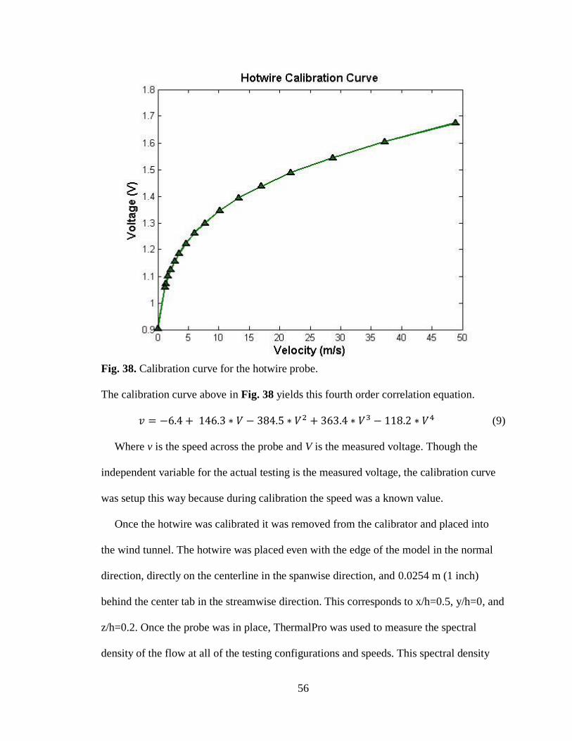
Fig. 38. Calibration curve for the hotwire probe.

The calibration curve above in Fig. 38 yields this fourth order correlation equation.

(9)

Where v is the speed across the probe and V is the measured voltage. Though the

independent variable for the actual testing is the measured voltage, the calibration curve

was setup this way because during calibration the speed was a known value.

Once the hotwire was calibrated it was removed from the calibrator and placed into

the wind tunnel. The hotwire was placed even with the edge of the model in the normal

direction, directly on the centerline in the spanwise direction, and 0.0254 m (1 inch)

behind the center tab in the streamwise direction. This corresponds to x/h=0.5, y/h=0, and

z/h=0.2. Once the probe was in place, ThermalPro was used to measure the spectral

density of the flow at all of the testing configurations and speeds. This spectral density

57

measures the fluctuations in the flow by comparing the frequency to the magnitude of the

measured voltages. The spectral density was then converted into the Strouhal Number

using Equ. (12) and the energy spectrum using Equ. (13).

(12)

where f is the frequency measured in ThermalPro, h is the height of the model 0.127 m (5

inches), and U∞ is the free stream velocity.

(13)

where ES is the normalized energy spectrum, E(f) the spectral energy measured in

ThermalPro and U∞ the free stream velocity.

Fig. 39. Energy spectra results for 10 m/s speed for all four tab configurations.

58

Fig. 39 shows the energy spectrum of the wake flow behind the model for the 10 m/s

test cases. For all four tab configurations there is a large spike close to the Strouhal

number of 0.21. The large width of the spike is due to the low resolution of the energy

spectrum at lower Strouhal Numbers. This large spike shows that there is a vortex

forming in the wake of the model. This data matches the base pressure data because it

shows that a vortex was shedding for all of the test cases. This result validates the results

from the base pressure tests because it shows that the vortex is not attenuated with the

tabs.




number of 0.18. As with previous experiments the spike moves slightly to the left and

59

becomes narrower with the increase in speed from 10 m/s to 20 m/s. The spike is

narrower than the 10 m/s tests because the data resolution increases with an increase in

Strouhal Number. This large spike shows that there is a vortex forming in the wake of the

model. This data matches the base pressure data because it shows that a vortex is

shedding for all of the test cases. This result validates the results from the base pressure

tests because it shows that the vortex is not attenuated with the tabs.




number of 0.19. As with previous experiments the spike moves slightly to the right and

becomes thicker with the in increased speed from 20m/s to 30 m/s. This large spike

shows that there is a vortex forming in the wake of the model. This data is aligned with

60

the base pressure data because it shows that a vortex is shedding for all of the test cases.

This result validates the results from the base pressure tests because it shows that the

vortex is not attenuated with the tabs. Though the hotwire tests were not necessary

because of the results from the base pressure tests, the hotwire tests act as a second

source to prove that the tabs did not attenuate the vortex for this experiment.

61

7. DISCUSSION

The results with the addition of the low, medium, and high tabs for the square base

pressure tests, the sting balance tests, and the hotwire energy spectra tests all suggest that

the tabs increase vortex strength instead of reducing it. This is apparent by the decrease in

average base pressure, the increase in total drag and the existence of a large spike in the

hotwire energy spectrum.

In the experiment by Park et al. [3], it was shown that the vortex was attenuated by

the increase of the wake width behind the test model. This increase in wake width was

caused by the generation of streamwise vortices created by the tabs. The addition of the

tabs in previous experiments [3,6] resulted in an increase in base pressure. In the 2D bluff

base case, the tabs prolong the formation of the vortex, decrease the suction on the model

and thus increase the base pressure [3]. In the rectangular bluff base with an aspect ratio

of four, the base pressure was reported to be increased by adding tabs only on the long

side of the base [6]. This base pressure recovery was not observed in this experiment.

In Pinn’s experiment the vortices in the normal direction (normal vortices) were four

times longer than the vortices in the spanwise direction (spanwise vortices) and the

normal vortices were much weaker so controlling vortices only in the normal direction

was sufficient to prolong the vortex formation [6] for the lower test speeds. For the

present experiment, however, the spanwise and normal vortices are equal in length and

almost equal in strength due to the similar boundary layer vorticity development. The

equality in length is shown in Fig. 42 and the similarity in strength can be seen in the

base pressure testing in Fig. 28 -Fig. 35.

62

Fig. 42. Comparison of model aspect ratios.

In this case the conjecture is that when the tabs are introduced in only the normal

direction, the edges of the two side tabs (the tabs close to the edges of the square base)

produce vortices which are close to and in the same directions as the spanwise vortices,

illustrated in Fig. 43 below. As a result, the strength of the spanwise vortices increase, as

do the strength of the normal vortices. The resulting decrease in base pressure causes the

increase in drag. Therefore, for the square base model, further study needs to be done

with the tabs introduced in both the normal and spanwise directions to show its drag

reduction effect and possibly in different tab locations.

Fig. 43. Schematic of vortices.

63

8. CONCLUSIONS

A square base bluff body was tested in the Cal Poly 3 x 4 ft low-speed wind tunnel.

The tests aimed to show the effectiveness of adaptive end plate tabs to reduce drag on the

bluff body model. The goal of the tabs was to increase the base pressure and decrease the

mean drag while attenuating the vortex shedding in the wake of the model. Unlike Pinn’s

experiment on a bluff body with the aspect ratio equal to 4, by merely disturbing the

vortex with tabs in the spanwise direction, no drag reduction was found. For the present

model with aspect ratio equal to 1 though, the tabs increased the drag on the model at all

three tested Reynolds numbers. This analysis was done by first measuring the boundary

layer on the trailing edge of the model to find the optimal tab height. The base pressure

was then tested to see the effects of the tabs on the base pressure. Next a total force

measurement was taken at all speeds and tab configurations to calculate the total drag on

the model. Finally a hotwire probe was used to measure the velocity fluctuations in the

wake flow near the model. These tests were done at speeds of 10, 20, and 30 m/s which

correlate to Reynolds numbers of 8.3e4, 1.6e5 and 2.5e5. The three conclusions are as

follows:

1. Base pressure measurements showed a decrease in base pressure at an average of

0.0449, 0.0398, and 0.0394 for 10, 20, and 30 m/s respectively by adding the tabs

to the trailing edge. This correlates to an increase in mean drag. Base pressure

testing also showed an increase in vortex strength instead of a decrease due to

larger valleys in the Cpb data.

2. Direct total drag force measurements also showed an increase in overall drag of

the model with the addition of the tabs for all tab heights and test speeds.

64

3. Hotwire data showed that the vortex is present with and without the tabs. This

result was shown by a large spike in the energy spectrum near a Strouhal number

of 0.2.

In previous works it was shown that the mechanism for drag reduction by tabs was to

increase the wake width between the tabbed edges [3]. While it appears the flow was

altered with the addition of the tabs on the present model, the drag was still increased.

This was possibly due to the strengthening of spanwise vortices. For future testing in this

field, tabs should be added to all four edges of the low aspect ratio bluff body at different

locations in order to see the tab effects in attenuating the vortices.

65

REFERENCES

1 Bearman, P. W. Investigation of the flow behind a two-dimensional model with a

blunt trailing edge and fitted with splitter plates. J. Fluid Mech. (1995), 241-255.

2 Bearman, P. W. The Effect of Base Bleed on the Flow behind a Two-Dimensional

Model with a Blunt Trailing Edge. The Aeronautical Quarterly Vol. XVIII (1967),

207-224.

3 Park, H, Lee, D, Jeon, W-P, Hahn, S, and Kim, J. Drag reduction in flow over a two-

dimensional bluff body with a blunt treailing edge using a new passive device. The

Journal of FLuid Mechanics (2006), 389-414.

4 Knight, James and Tso, Jin. A Comparison of Bluff-Body Base-Drag Reduction By

Passive Control Means. Ontario, 2005.

5 Knight, James. Drag Reduction for Reusable Launch Vehicles Through Boundary

Layer Extraction. 2003.

6 Pinn, Jarred. Effect of End-Plate Tabs on Drag Reduction of a 3D Bluff Body with a

Blunt Base. San Luis Obispo, 2012.

7 Carlson, Charles and Innes, Paul. Test and Verification of Vortex Shedding for a 3D

Bluff Body. San Luis Obispo, 2012.

8 Erlhoff, Ethan. Distributed Forcing on A 3D Bluff Body With A Blunt Base An

Experimental Active Drag Control Approach. San Luis Obispo, 2012.

9 IFA 300 Constant Temperature ANemometer System Instruction Manual. TSI

Incorporated, St. Paul, 2000.

10 Pope, Alan. Wind-Tunnel Testing. John Wiley & Sons, New York, 1954.

11 Taylor, John R. An Introduction to Error Analysis: The Study of Uncertainties in

Physical Measurements. University Science Books, 1997.

66

APPENDICES

A. Sample Error Calculations

The following calculations were derived from methods by Taylor [11].

(

)

| |√(

)

[(

)

]

(

)

| |

√

(

)

[(

) ]

(

)

Similarly,

Neglect A, so

So

| |√(

)

(

)

(

)

| |√(

)

(

)

(

)

67

B. Sample Pressure Code

%% Base Pressure Profile

loadraw=0; %toggle loading raw or cached data shownorm=1; %toggle normal showspan=1 %toggle spanwise showtabs=1;%show based on tab with varying speeds showtabs2=1;

%line colors for each test color(1,:)='-bo'; color(2,:)='-r^'; color(3,:)='-gs'; color(4,:)='-ko'; clr=[1 0 0;0 .5 0; 0 0 1;0 0 0];

%directory for tests test(1,:) = 'NoTab'; %base test(2,:) = 'HiTab'; %10 m/s opt test(3,:) = 'MeTab'; %20 m/s opt test(4,:) = 'LoTab'; %30 m/s opt

%creates locations of ports (can be location or port numbers) x=[4.875 4.75 4.5 4.25 4 3.5 3 2.5 2 1.5 1 .75 .5 .25 .125]; %(0,0) at

bottom left corner as mounted x=x-2.5; %sets (0,0) to center of model x=x/5; x1=x; % x=(1:15); %sets x to port numbers

% Declare Variables CP=zeros(4,3,45); press=CP; CPNose=zeros(4,3); avgcp=zeros(4,3); difavgcp=avgcp; lw=2; %set the line width for plots fs=12; %chart font size ts=12; %chart title size fw='Bold'; %set chart font weight tw='Bold'; %set chart title font weight

casest=[1 2 3 4]; %Set Tab heights casess=[1 2 3]; %Set Speeds

load('BPData.Mat')

for t=1:4 %tab configurations for s=1:3 % speeds (1=10, 2=20, 3=30) if loadraw==1 %loadcase(t,s)==1 file=['Base Pressure\',test(t,:),'\Base',num2str(s),'.dat'] [CP2(1:30),press2(1:32)]=Pressure_Data(file,32);

%Shift Ports

68

CP(t,s,1:30)=CP2(1:30); CPNose(t,s) = CP2(15); %check stagnation point ~.98 CP(t,s,8)=CP2(23); %port in very center of base plate press(t,s,1:32)=press2(1:32); press(t,s,8)=press2(23); end end end

%% Display Results Based On Speed if shownorm==1

for s=casess figure(s) hold on for t=casest y(1,1:15)=CP(t,s,1:15);

plot(x,y,color(t,:),'Color',clr(t,:),'LineWidth',lw,'MarkerFaceColor',c

lr(t,:),'MarkerEdgeColor',[0 0 0]); end title(['Base C_P Data for ',num2str(s),'0 m/s

Test'],'FontSize',ts,'FontWeight',tw) xlabel('Normal Position, y/h','FontSize',fs,'FontWeight',fw) ylabel('C_P_b','FontSize',fs,'FontWeight',fw) axis([-.5 .5 -.4 -.15]) legend('No Tabs','High Tabs','Medium Tabs','Low

Tabs','Location','SouthEast') end end

if showspan==1 % figure(4) %plot Spanwise Data for s=casess figure(s) hold on for t=casest x=x1; y(1,1:15)=CP(t,s,16:30);

plot(x,y,color(t,:),'Color',clr(t,:),'LineWidth',lw,'MarkerFaceColor',c

lr(t,:),'MarkerEdgeColor',[0 0 0]); end title(['Base C_P Data for ',num2str(s),'0 m/s

Test'],'FontSize',ts,'FontWeight',tw) xlabel('Spanwise Position, x/h','FontSize',fs,'FontWeight',fw) ylabel('C_P_b','FontSize',fs,'FontWeight',fw) % set(gca,'YDir','reverse'); axis([-.5 .5 -.4 -.15]) legend('No Tabs','High Tabs','Medium Tabs','Low

Tabs','Location','SouthEast') end

end

69

%% Plot based on tab heights test2=['No Tabs ';'High Tabs';'Med Tabs ';'Low Tabs ']; if showtabs==1

x1=x; figure(6) for t=casest % figure(t+5) subplot(2,2,t) for s=casess x=x1; y(1,1:15)=CP(t,s,1:15);

plot(x,y,color(s,:),'Color',clr(s,:),'LineWidth',lw,'MarkerFaceColor',c

lr(s,:),'MarkerEdgeColor',[0 0 0]); hold on end

title(['Base C_P Data for ',test2(t,:),'

Test'],'FontSize',ts,'FontWeight',tw) xlabel('Normal Position, y/h','FontSize',fs,'FontWeight',fw) ylabel('C_P_b','FontSize',fs,'FontWeight',fw) axis([-.5 .5 -.4 -.15]) legend('10 m/s','20 m/s','30 m/s','Location','SouthEast') end end

if showtabs2==1 figure(7) for t=casest % figure(t+5) subplot(2,2,t) for s=casess x=x1; y(1,1:15)=CP(t,s,16:30);

plot(x,y,color(s,:),'Color',clr(s,:),'LineWidth',lw,'MarkerFaceColor',c

lr(s,:),'MarkerEdgeColor',[0 0 0]); hold on end

title(['Base C_P Data for ',test2(t,:),'

Test'],'FontSize',ts,'FontWeight',tw) xlabel('Spanwise Position, y/h','FontSize',fs,'FontWeight',fw) ylabel('C_P_b','FontSize',fs,'FontWeight',fw) axis([-.5 .5 -.4 -.15]) legend('10 m/s','20 m/s','30 m/s','Location','SouthEast') end end

C. Sample Boundary Layer Code

clc; clear all;close all; format compact fs=12; %chart font size

70

ts=12; %chart title size fw='Bold'; %set chart font weight tw='Bold'; %set chart title font weight

%% Boundary Layer ld=1; %0=process new data - 1=load processed data pl=1; %0= dont plot BL - 1=plot BL

load 'BLData.mat'

%calculate d* for 10 m/s y10=(1-V10/vfree10); ds10=abs(trapz(y10,h10));

%calculate momentum thickness for 10 m/s y102=V10./vfree10.*(1-V10./vfree10); th10=abs(trapz(y102,h10));





%combine into one vector dstar=[ds10 ds20 ds30]; theta=[th10 th20 th30]; H=dstar./theta; %check to see if its turbulent (<1.5)

%find tab heights th1=dstar*2; Tab_Heights=theta*3 Tab_Height_2x=theta*2; Tab_Height_1x=theta*1;

steps=[38,25,24]; V(1,1:38)=V10./vfree10; V(2,1:25)=V20./vfree20; V(3,1:24)=V30./vfree30; P(1,:)=polyfit(V(1,1:38),h10,4); P(2,:)=polyfit(V(2,1:25),h20,4); P(3,:)=polyfit(V(3,1:24),h30,4);

%find boundary layer

71

for i=1:3

delta(i)=P(i,5)+.995*P(i,4)+.995^2*P(i,3)+.995^3*P(i,2)+.995^4*P(i,1); end

h(1,1:38)=h10/delta(1); h(2,1:25)=h20/delta(2); h(3,1:24)=h30/delta(3);

test=['10 m/s';'20 m/s';'30 m/s'];

if pl==1 %plot non-dimensional boundary layers for q=1:3 figure(q) plot(V(q,1:steps(q)),h(q,1:steps(q)),'-

bo','LineWidth',2,'MarkerFaceColor','b','MarkerSize',3) hold on title(['Boundary Layer Profile for ',test(q,:),'

Test'],'FontSize',ts,'FontWeight',tw) xlabel('Velocity (u/U_\infty)','FontSize',fs,'FontWeight',fw) ylabel('Height (y/\delta)','FontSize',fs,'FontWeight',fw) axis([0 1.2 0 1]) end end

Effect of Adaptive Tabs on Drag of a Square-Base Bluff Body

Documents

Transcript of Effect of Adaptive Tabs on Drag of a Square-Base Bluff Body