EEG measurements,

experimental design and

preprocessing

Chapter 4

BING 8995Dr. Vidya Manian

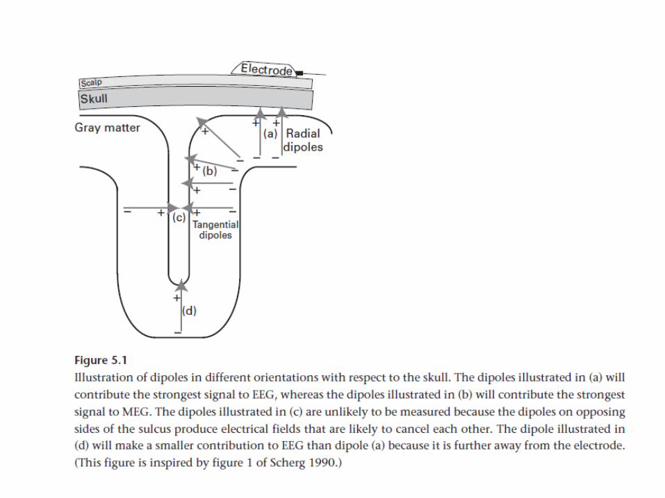
• EEG electrodes measure sum of electric potential from 10,000 to 50,000 neurons in superficial cortical layers

• There is sufficient electrical conductivity from neuron population to scalp. Air has 0 conductivity, so gel is normally used to make electrode contact on the scalp

• Dozens of trials are sufficient for cortex-generated potentials

• Deep brain sources such as thalamus, basal ganglila, hippocampus and brainstem are difficult to measure on scalp.

• There should be many trials for averaging. For brainstem generated potentials, 1000s of trials is needed to obtain good SNR (Signal-to-Noise-Ratio)

• To measure activity in deep brain structure using scalp EEG, use a task that is known to elicit activity in that brain region, have many trials (100s or 1000s)

• Perform source localization to support the origin of the deep brain source, use many electrodes, and subject specific anatomical MRIs to increase spatial accuracy of the source reconstruction result

• Slow fluctuations <1 Hz and fluctuations >100 Hz are difficult to measure with EEG, but not impossible

• EEG activity >80 Hz may be driven by noise spikes, EMG, eye movement or other artifacts

Phase locked, time locked and task related

• Phase-locked activity (also sometimes called “ evoked ” ) is phase-aligned with the time = 0 event and will therefore be observed both in time-domain averaging (the ERP) and in time-frequency-domain averaging

• Non-phase-locked activity (also sometimes called “ induced ” ) is time-locked but not phase-locked to the time = 0 event

• Non phase locked activity can be seen in time-frequency domain averaging, not in time-domain averaging and has no representation in ERP

• Both are task related, their time/frequency characteristics change as a function of engagement in task events

• Background activity is used in resting state studies. In cognitive electrical physiology it has little useful information

• It can be removed by baseline normalization, allowing focus on task-related dynamics

Neurophysiological mechanisms of ERP (event related potentials)

• why there are positive and negative polarity peaks at somewhat regularly spaced intervals following experiment events?

• Additive: ERP reflects a signal that is elicited by an external stimulus such as a picture or a sound or by an internal event such as the initiation of a manual response and is added to ongoing background oscillations, which are attenuated by trial averaging

• Phase reset: when a stimulus appears, the ongoing oscillation at a particular frequency band is reset to a specific phase value, which may reflect a return to a specific neural network configuration

• Several lines of evidence suggest that electrical fields are causally involved in neural computation and information transfer

• Evidence comes from in vitro studies of LFP (local field potential) oscillations and synaptic events thought to underlie learning and memory

• long-term potentiation in the hippocampus, which is thought to be a basis of Hebbian learning and thus memory formation, occurs preferentially at specific phases of theta-band (4 – 8 Hz) oscillations

• Interregional oscillatory synchronization is a mechanism underlying the transmission of information across neural networks and that this synchronization-mediated connectivity is crucial for perceptual and cognitive processes

• Phase-based synchronization methods are the most widely used approaches for studying connectivity in electrophysiology data

Transcranial alternating current stimulation (TACS)

• TACS is passing a current between electrodes placed on the scalp, frequency between 0.1 and 100 Hz

• Stimulation at an individual subject ’ s alpha peak increased alpha power• TACS is not often used in cognitive electrophysiology but may become an

important tool for testing hypotheses about the role of specific oscillation frequencies in cognition

• Are electric fields causally involved in cognition?• Electrical fields produced by neural populations are undeniably powerful

and insightful indices of brain function• BOLD is not a causal mechanism of brain information processing, but

BOLD response is a powerful and useful indirect index of brain function• If there is conclusive evidence against a causal role of oscillations in

cognition, it would not stop cognitive electrophysiologists from using EEG to make important discoveries about the functional organization of cognition and the brain

Experiment Design

• Well designed experiment is more important than noisy data and basic analyses

• Pilot test the experiment behaviorally to make sure you obtain the predicted behavior

• Analyze the pilot dataset to find suboptimal and fixable design features during piloting itself

Event markers

• Event markers or triggers are square wave pulses sent from stimulus delivering computer to the EEG amplifier and are recorded as a separate channel in the raw data file

• Amplitude is used to encode stimulus onset or response• During data importing, the markers are converted to

labeled time stamps that indicate when different events in the experiments occurred

• Event markers are used to time-lock the EEG data offline• A pair of markers spaced 10ms apart provides 65,025

possible unique markers (255 times 255)

Duration of marker

• a 0.5-ms marker might not be recorded if the sampling rate is 500 Hz, if the markers have a duration of 200 ms, they are likely to overlap with other markers

• 5 ms should be a sufficient duration

• Psychophysics toolbox of Matlab: deliver stimuli to subject and event marker to EEG data acquisition system

Intra and intertrial timing

• time-frequency responses may linger for hundreds of milliseconds after an experiment event has ended, it is ideal to have experiment events within a trial separated by at least several hundred milliseconds

• brain response to one event should subside before the response to the next event begins

• time-frequencydynamics elicited by a simple and neutral visual stimulus, such as a Gabor patch, will likely decay quickly after stimulus offset.

• But the time-frequency dynamics elicited by a picture ofa sick child in a poor country might take longer to subside because of lingering reactions to that picture

Intertrial interval

• Time between the end of one trial and start of another trial

• baseline time period for time-frequency decomposition should end before trial onset, for example – 500 to –200 ms

• Temporal filtering may cause post-stimulus activity to ‘leak’ into pre-stimulus activity

• for ERPs the baseline period typically ends at the time = 0 event

• For most cognitive electrophysiology experiment designs, intertrial intervals of at least 1000 ms should be sufficient

How many trials

• Depends on SNR, how big the effect is, and type of analysis

• a minimum of 50 trials per condition per subject is a reasonable number of trials that should lead to a sufficient level of SNR

• For P3 amplitude, only 3 electrodes are needed (one placed over parietal central cortex to recordP3, one ground, and one reference)

• To test for 50 Hz activity, sample at 100 Hz• Sampling rates between 500 Hz and 2000 Hz are

likely to be sufficient for all analyses

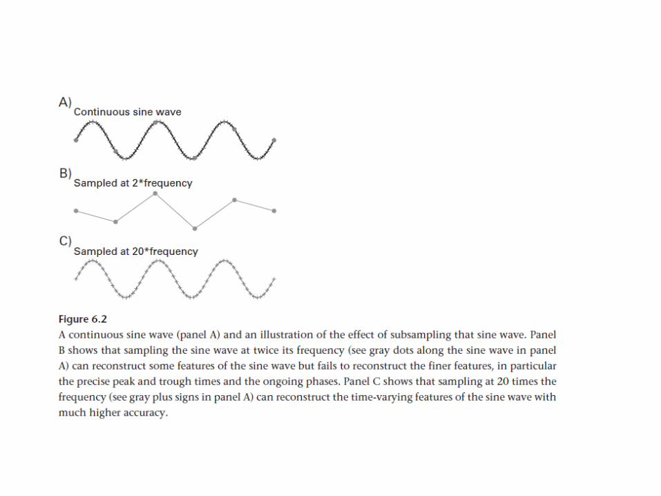
• At 1000 Hz, there is a one-to-one conversion between time in ms and time in samples. That is, 14 ms is also 14 samples. 500 and 2000 Hz are the next-most convenient sampling rates (14 ms is, respectively, 7 and 28 samples)

• Additional devices: EMG, eye tracker, electrode localization equipment, a comfortable chair for the subject to sit in, a good response device

Balance between signal and noise

Preprocessing

• Preprocessing refers to any transformations or reorganizations that occur between collecting the data and analyzing the data

• Some preprocessing steps merely organize the data to facilitate analyses without changing any of the data (e.g., extracting epochs from continuous data)

• other preprocessing steps involve removing bad or artifact-ridden data without changing clean data (e.g., removing bad electrodes or rejecting epochs with artifacts), and some

• preprocessing steps involve modifying otherwise clean data (e.g., applying temporal filters or spatial transformations)

• Amplifier saturations, for example, produce large spikes that are several orders of magnitude bigger than the neurally generated EEG. This has to be removed

• LP filtering of 30 Hz removes high frequency activity and muscle artifacts• Some researchers focus on 30Hz activity• Some remove ERPs as they consider it noise and need local stationarity• Some study only ERPs• One researcher’s noise is another researcher’s signal!!• Your preprocessing will depend on your criterion for balancing signal and

noise from temporal filtering, to trial rejection, to independent component analysis based rejection, to oculomotor based rejection

• If the experiment design is easy and you can take 100s of trials, there is the luxury of rejecting noisy data

• If the measurements are intracranial and difficult to record, some noise can be allowed

• Time frequency analysis increases SNR characteristic of the data particularly for single trial analyses and low frequencies

Creating Epochs

• EEG data is a 2D matrix (time and electrodes)• The continuous data are cut into segments surrounding

particular experiment events• the time-domain data are stored in a 3-D matrix

(electrodes, time, and trials)• what to call “ time = 0, could be stimulus onset at each trial

is a time =0• Several stimuli are presented with variable delay, multiple

events, time lock to the earliest event in each trial• how much time to include before and after the time = 0

event. Epochs should be atleast as long as the duration of the trial

For ERPs, – 200 ms until 800 ms relative to stimulus onset might sufficeFor time-frequency analysis create longer epochs, to avoid contaminating result with edge artifactsExtra ‘buffer zones’ is to have long epochs that allow the edge artifacts to subside before and after the experiment eventsTo analyze the time period from 0 to 1000 ms, you might take epochs from – 1500 to +2500 msThree cycles at the lowest frequency that will be analyzed is sufficientfor a buffer zone (e.g., 1500 ms for 2-Hz activity)

Data reflection

• Trial counts: Experiment design should be such that there are similar numbers of trials in each condition

• Filtering: helps remove high-frequency artifacts, low-frequency drifts, notch filters at 50 or 60 Hz

• HP filtering at 0.1 and 0.5 Hz is useful to minimize slow drifts• High-pass filters should be applied only to continuous data and not

to epoched data• Trial rejection: Removing trials that contain artifacts prior to

analyses is an important preprocessing step• sharp edges in the data are more detrimental to time-frequency

decomposition than they are to ERPs, relatively small sharp edges can have adverse effects on time-frequency decomposition results

Spatial filtering

• To help localize a result. Eg., activity peak corresponds to left motor cortex, then apply a surface Laplacian or fit a single dipole

• task involves visual stimuli that require spatial attention, it may be difficult to separate visual processing in occipital cortex from attention-related processing in parietal cortex

• the surface Laplacian or distributed source imaging may help minimize the spatial overlap between occipital and parietal responses, thereby increasing confidence in functional/anatomical distinctions– Helps remove volume conduction, which may contaminate

connectivity analyses– Can be applied before or after time-frequency decomposition; for ERP

study a single dipole can be fit to the grand averaged ERP– For connectivity, surface Laplacian can be applied before time-

frequency decomposition and connectivity is computed

Referencing

• Averaged mastoids (the bone behind the ear) or earlobes are typical reference electrodes. (The sample data for the assignment are referenced to linked earlobes.)

• The reference electrode should not be close to an electrode where you expect the main effects. For example, Cz is a poor choice of reference if the analyses involve response errors (which elicit maximal activity around electrode Cz or FCz)

Interpolating bad electrodes

• Bad electrodes can be interpolated with data from neighboring electrodes

• Not recommended, better to inspect data and remove the bad electrode

• One way to determine whether a noisy electrode contains brain signal is to apply a low-pass filter to the data at 30 Hz. If the low-frequency activity from that electrode looks similar to that of the surrounding electrodes, the unique signal from that electrode can be salvaged

• Clean data with high SNR is the best!!

EEG artifacts, their detection and removal

• blinks, muscle movements, brief amplifier saturations, and line noise

• high-frequency activity may look like noise at the single-trial level, and non-phase-locked activity may look like noise when one is computing an ERP

• Most EEG data analyses are robust to the levels of noise that are typically observed in EEG data (after preprocessing), particularly with dozens or hundreds of trials per condition

Removing data based on ICA

• the independent components analysis provides a set of weights for all electrodes such that each component is a weighted sum of activity at all electrodes, and the weights are designed to isolate sources of brain electrical signals

• ICA can be used to clean data; isolate artifacts and subtract those components from the data or as a data reduction technique

• When independent components analysis is used as a preprocessing tool, components can be judged as containing artifacts based on their topographies, time courses, and frequency spectra. Components containing blink artifacts are probably the easiest to identify

• take a conservative approach and remove components from the data only if you are convinced that those components contain artifacts or noise and no or very little signal

• In the best-case scenario we would remove only one component corresponding to blink artifacts

Removing trials because of blinks

• Trials containing blinks should not be rejected• They can be removed by ICA• They should avoid time-locking their blinks to

experiment events such as button presses or stimulus offsets to facilitate a clean statistical isolation of blink artifacts from the experiment events to which those blinks are time-locked

• if subjects always blink whenever they press a button, it will be difficult for an independent components analysis to isolate the blink activity from the response-related activity (because these will not be independent components)

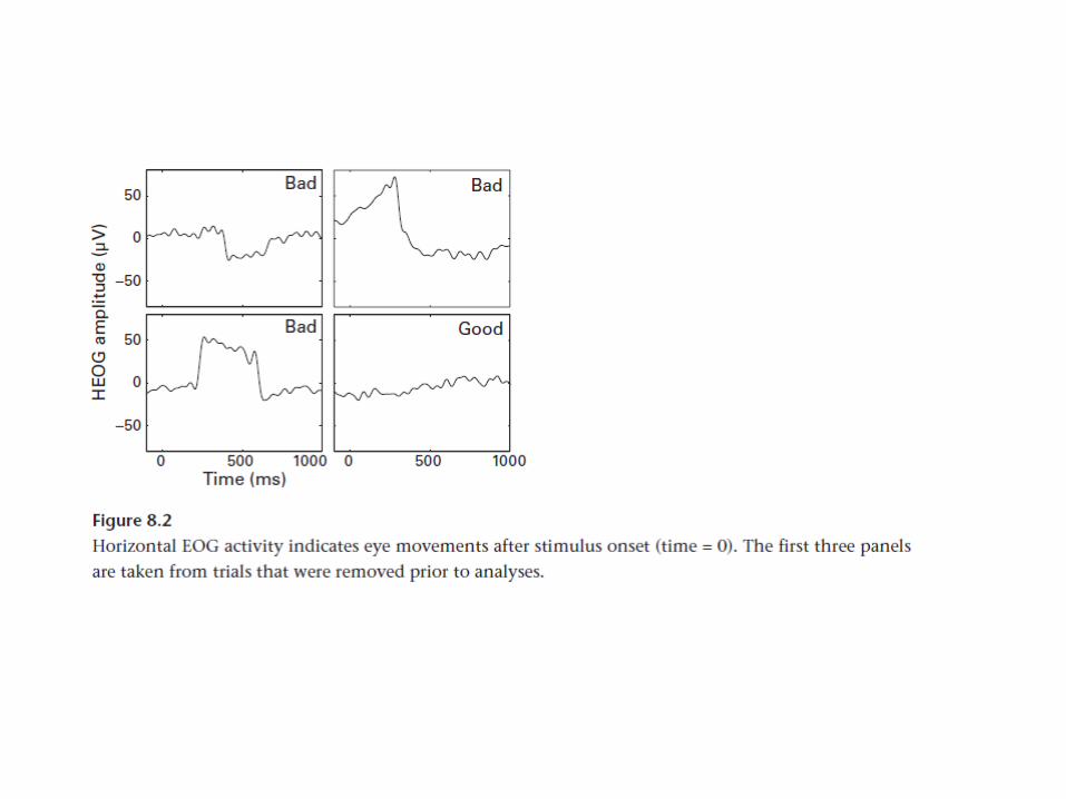
Removing trials because of oculomotor activity

• There are also saccades and microsaccades that can contaminate EEG data, particularly at frontal and lateral frontal electrodes (or at posterior electrodes if the reference electrode is on the face)

• Have visual stimuli at a central location on the experiment monitor

• Instruct subjects that small eye movements cause artifacts in the data will help minimize the frequency of saccades

• The potential impact of microsaccades on high-frequency EEG activity is a recent topic of discussion

• Microsaccades can be minimized by having small stimuli such that subjects do not need to saccade to see the entire stimulus, and by presenting the stimulus on the screen for only a short period of time (this may not be feasible in all experiments). There are algorithmic approaches for detecting and removing microsaccade artifacts from EEG data

• If main hypotheses concern anterior frontal or lateral frontal regions, EOG artifacts are a serious concern;

• if main hypotheses concern midcentral electrodes, EOG artifacts are less of a concern because they are less likely to be measured at these electrodes

• Spatial filtering techniques can help isolate potential EOG artifacts. The surface Laplacian, for example, will help prevent the spread of oculomotor artifacts to activity at other electrodes

Removing trials based on EMG in EEG channels

• Trials with excessive EMG activity in the EEG channels should be removed. EMG is noticeable as bursts of 20- to 40-Hz activity, often has relatively large amplitude, and is typically maximal in electrodes around the face, neck, and ears

• EMG bursts are not good for analyzing data above 15 Hz, means the subject moved, coughed, sneezed or giggled during the trial

• If hypothesis is about beta-band activity, cannot use dataset with continuous EMG

Removing trials based on task performance

• Remove trials with more responses than required, with very fast reaction times (for a finger button press, less than 200ms), and trials with slow reaction times

• Remove trials with cognitive noise or cognitive artifacts

• if subjects perform a few tens of trials with one set of instructions and then switch to another set of instructions; the first trial after each switch will involve a cognitive set shift and a switch cost

• Also, in the trial after a long break, the subject may not be fully reengaged

Removing trials based on response hand EMG

• Recording EMG from the thumb muscle tends to be easier than EMG from the other fingers

• have subjects use response buttons that take some effort to press. This produces bigger and cleaner EMG responses.

• In contrast, a mouse button requires little physical exertion to press and will produce a small EMG activation

Train Subjects to Minimize Artifacts

• Many EEG artifacts can therefore be minimized with proper training

• Explain that EEG data contain both brain activity and noise from muscles.

• You can have him/her blink, clench her jaw, tense her neck/shoulder muscles, talk, smile, wiggle and so on.

• When subjects know what kinds of behaviors produce EEG artifacts, they can minimize those behaviors during the task

• The best way to get your preprocessing protocol to turn good data into very good data is to start with good data

• At least once every 30 s you should quickly glance at the EEG data and check that they look OK

• If the artifacts are present during the task, consider pausing the experiment at the next possible opportunity to determine what is causing the artifacts

• If the artifacts are coming from the subject being tired or uncomfortable, turning the lights on and talking to the subject for a minute before resuming the task might help to reengage the subject ’ s attention and reduce the source of the artifacts

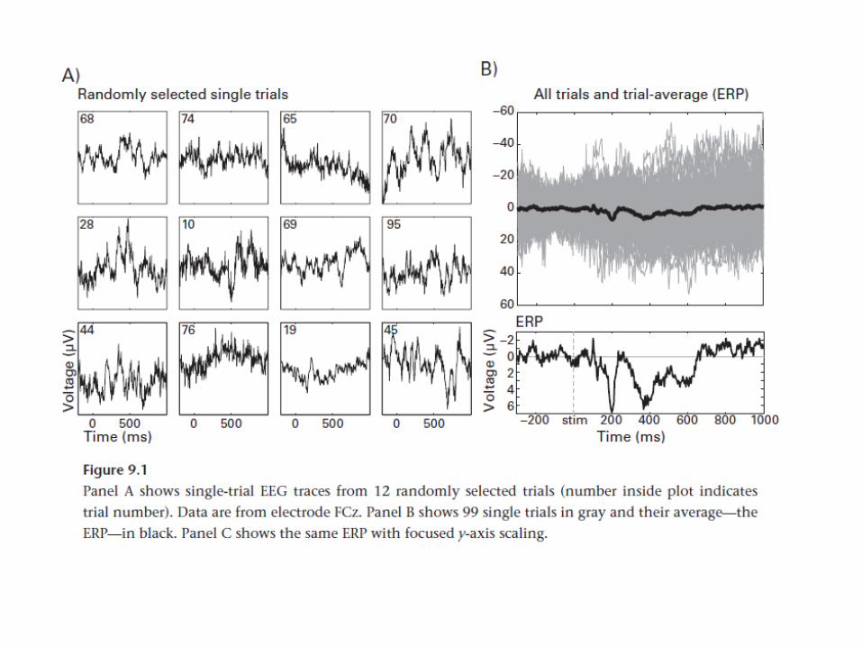
Time domain EEG analyses-Event Related Potentials (ERPs)

• Because the noise fluctuations are randomly distributed around zero, noise cancels out when many trials are averaged, thus leaving the signal (the ERP)

• To create an ERP, simply align the time-domain EEG to the time = 0 event (this was probably already done during preprocessing) and average across trials at each time point

• sum the voltage at each time point over trials and then divide by the number of trials

• For using ERPs to make inferences about cognitive processes, issues related to component overlap, component quantification, appropriate interpretation, and statistical procedures have to be considered

Filtering ERPs

• time-domain signal averaging over trials is itself a low-pass filter• because non-phase-locked activity does not survive time-domain averaging and

frequencies above around 15 Hz tend to be non-phase-locked• Filtering the ERP minimizes residual high-frequency fluctuations, makes the ERPs

look smoother, and facilitates peak-based component quantification by reducing the possibility that the peak is a noise spike or an otherwise non representative outlier

• Filters with narrow transition zones cause ripples in time domain that appear to be oscillations, construct filters with gentle transition zones

• The lower the cutoff frequency of the filter, the more temporal precision is lost. Because of these considerations, you should carefully consider whether a filter is necessary for your ERPs

• ERPs are often filtered using a frequency cutoff of around 20 or 30 Hz, and occasionally the frequency cutoffs are as low as 5 or 10 Hz

• Note that applying a filter to single trials and then computing the ERP is identical to computing the ERP and then applying a filter

• Filtering the data before trial averaging is thus not necessary, although it can be useful for data inspection or independent components analysis.

Butterfly plots and global field power / topographical variance plots

• Shows ERPs of all electrodes in the same figure• the butterfly plot will show ERPs symmetric about the

zero horizontal line. Butterfly plots are useful for detecting bad or noisy electrodes

• The global field power is the standard deviation of activity over all electrodes. Global field power can be obtained simply by computing the standard deviation over all electrodes at each point in time, and is best interpreted when using the average reference

• Butterfly plots and topographical variance plots are useful as data quality indices and to confirm the timing of the representations of task events in the data

The flicker effect

• entrainment of brain activity to a rhythmic extrinsic driving factor• if subject looks at a strobe light that flickers at 20 Hz, there will be

rhythmic activity in your visual cortex at 20 Hz, phase-locked to each light flash from the strobe light. This can be measured as a narrowband increase in power or phase alignment at the frequency of the visual flicker, or it can be measured in the ERP. This effect is also referred to as steady-state evoked potential, frequency tagging, SSVEP (steady-state visual evoked potential), SSAEP (auditory evoked potential)

• One limitation of the flicker effect is its poor temporal precision• it takes several hundred milliseconds for the flicker effect to

stabilize, and longer periods of time provide an increased signal-to-noise ratio. Thus, this approach is ideal for stimuli that can remain on screen for several seconds

In which brain region the flicker will entrain neural network activity

• theta-band visual flicker increases hemodynamic activity in medial prefrontal regions

• there is some evidence that performance on cognitive tasks can be modulated by stimulus flicker frequency

• entrainment can modulate processing of stimuli that are presented in phase compared to stimuli presented out of phase with the entrainment stream, brain retains frequency at which items are tagged

• Stimulus flicker frequencies up to 100 Hz can evoke a flicker effect,although lower frequencies generally elicit a stronger flicker effect (that is, larger in magnitude). Other stimulus factors such as size, luminance, and contrast will impact the signal-to-noise ratio of the flicker effect

• a peak in the frequency domain at the flicker frequency should be readily observed in a spectral plot, and the magnitude of this frequency peak can be compared to the same frequency before the flickering stimulus began, or it can be compared to the power of neighboring frequencies for which there was no flicker

• Can perform frequency decomposition or time-frequency decomposition

Topographic maps

• Shows spatial distribution of EEG results• Creating a topographical map is conceptually similar to

interpolating an electrode• Activity is estimated at many points in space between electrodes• The online Matlab code goes through, step-by-step, how

topographical maps are created• Easier to plot with eeglab, fieldtrip or other EEG analysis programs• The maps here are plotted using eeglab topoplot• ERP topographic maps can be used for rapid data inspection• Topographical maps allows confirming the timing• of task events, and they allow detection of bad or noisy electrodes

Microstates

• “In EEG as well as ERP map series, for brief, subsecondtime periods, map landscapes typically remain quasi-stable, then change very quickly into different landscapes ”

• Duration of landscapes around alpha range (70-130 ms), and topographical distributions tend to fit into four or five distinct patterns

• Microstates have been linked to cognitive processes from perception to memory to language, prestimulusinterval that predicts upcoming stimulus progression

• The software package cartool is designed for studying Microstates( sites.google.com/site/fbmlab/cartool)

To identify microstates

• Temporally stable topographical distributions, the difference between the topographical maps at times t and t + 1 is small

• when the temporal difference (also called global map dissimilarity) remains low for a period of tens to hundreds of milliseconds and then suddenly becomes relatively large, this sharp increase is considered to be a transition from one state to another

• The stable maps are then used in a hierarchical clustering analysis to identify a small number of topographical distributions that best characterize the topographical maps during periods of stability. These are called cluster maps.

• Topography at each time point is labeled according to the cluster map to which it is most similar. This produces a time course of map topographies and can be used in task-related and statistical analyses

ERP Images

• An ERP image is a 2-D representation of the EEG data from a single electrode

• the single-trial EEG traces are stacked vertically and then color coded to show changes in amplitude as changes in color

• ERP images can be used to link trial-varying task parameters or behaviors to the time-domain EEG signal

• sort the EEG trials according to values of the aligning event, such as the reaction time or the phase of a frequency-band-specific signal at a certain time point

• ERP images are often smoothed, for example by convolving the image with a 2-D Gaussian, to facilitate interpretation and to minimize the influence of noise or other nonrepresentative single-trial fluctuations

• eeglab has easy-to-use options for creating and smoothing ERP images

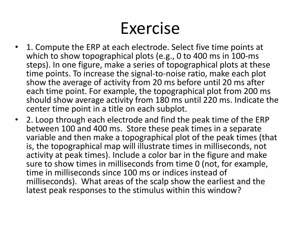
Exercise• 1. Compute the ERP at each electrode. Select five time points at

which to show topographical plots (e.g., 0 to 400 ms in 100-ms steps). In one figure, make a series of topographical plots at these time points. To increase the signal-to-noise ratio, make each plot show the average of activity from 20 ms before until 20 ms after each time point. For example, the topographical plot from 200 msshould show average activity from 180 ms until 220 ms. Indicate the center time point in a title on each subplot.

• 2. Loop through each electrode and find the peak time of the ERP between 100 and 400 ms. Store these peak times in a separate variable and then make a topographical plot of the peak times (that is, the topographical map will illustrate times in milliseconds, not activity at peak times). Include a color bar in the figure and make sure to show times in milliseconds from time 0 (not, for example, time in milliseconds since 100 ms or indices instead of milliseconds). What areas of the scalp show the earliest and the latest peak responses to the stimulus within this window?

Time frequency power and baseline normalization

• how to link fluctuations in power over time and frequency to task events

• 1/f power scaling• the frequency spectrum of data tends to show

decreasing power at increasing frequencies.• This is the case for EEG, radio, radiation from big bang,

natural images• power law: one variable (in this case, EEG time-

frequency power) is a power function of another variable (frequency)

• c/(f^x)

EEG time-frequency power obeys a 1/f phenomenon, the power at higher frequencies (gamma) has smaller magnitude than power at lower-frequencies (delta)Drawbacks1. Difficult to visualize power across a range of frequencies2. difficult to make quantitative comparisons of power across frequency bands3. Individual differences in raw power are influenced by skull thickness, sulcal anatomy, cortical surface area recruited, recording environment (e.g., scalp cleanliness and preparation and electrode impedance), and other factors.4. Task related changes in power can be difficult to disentangle from background activity5. Raw power values are not normally distributed because they cannot be negative and arestrongly positively skewed. This limits the ability to apply parametric statistical analyses totime-frequency power data

No color scale is adequate to show changes in all or even most frequency

bands

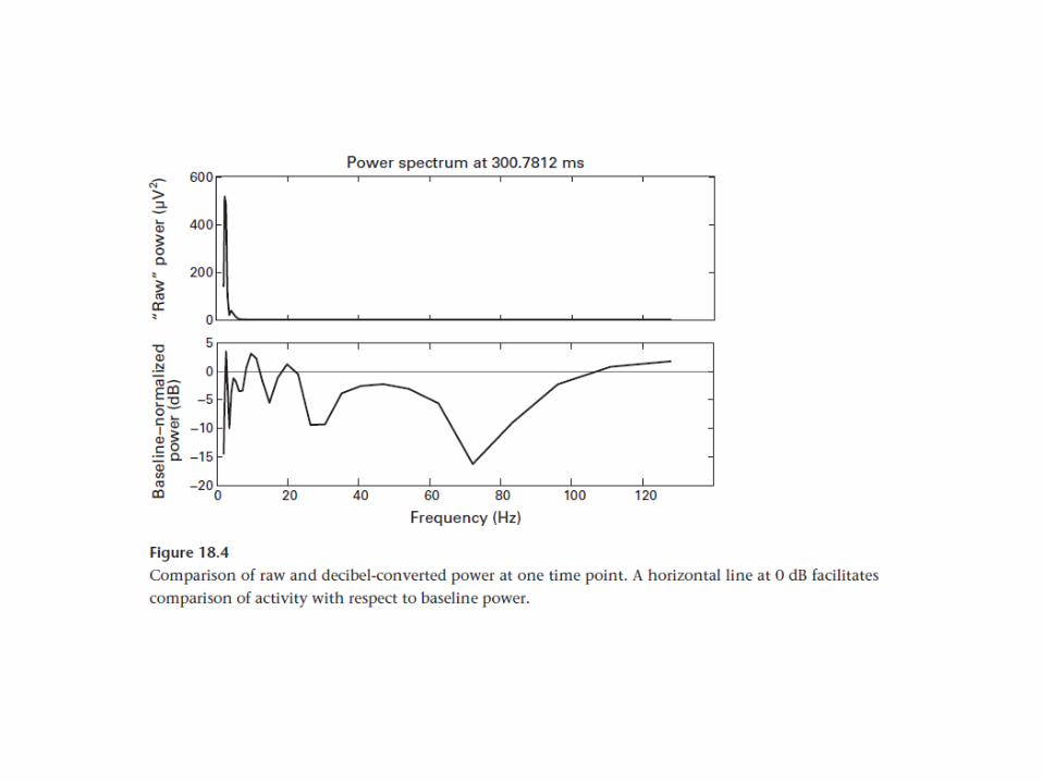
Advantage of baseline normalization

• They transform all power data to the same scale. This allows you to compare, visually and statistically, results from different frequency bands, electrodes, conditions, and subjects

• Because baseline-normalized power data are often normally distributed, parametric statistical analyses may be appropriate to use

• time-frequency dynamics become disentangled from background or task unrelated dynamics

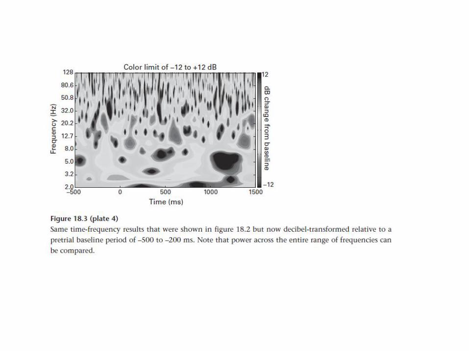
3 baseline normalization procedures

• Decibel conversion• The choice of baseline period is a nontrivial one

and influences the interpretation of your results• a baseline period of – 500 to – 200 ms before trial

onset is used• Typical decibel values after trial averaging are in

the range of ± 1 – 4 dB.• For real data analyses, decibel conversion should

be done on the trial-average power. That is, first average trials together and then transform to decibels;

Color scaling• symmetric color scaling should be preferred in

most situations. use – 3 to +3 or – 1.5 to +1.5 rather than – 3 to +1

Percentage change and baseline division

• A related transform to percentage change is dividing power during the task by power during the baseline time period

Comparison of different normalization methods

Mean and Median Power

Presence of outlier

Choice of baseline time period window

• in ERP analyses it is common to have the baseline end at time = 0• For time-frequency analyses, if activity occurs shortly after time = 0

event: a good baseline time period might be – 500 to – 200 ms, or –400 to – 100 ms

• any activity present in the baseline period will be transferred to the task-related activity, it is a good idea to use the pretrial period as a baseline event if you are not examining stimulus-locked activity

• A pretrial baseline period is optimal. Whenever possible, try to design your experiment such that a pretrial baseline period of several hundred milliseconds can be used

• One option is to use a separate rest period as the baseline, inform subject so there are no artifacts

• Baseline normalization is almost always a good idea but is not always necessary

SNR

µ is mean power over trials, sigma is the standard deviation of the power over trials,tf is one time frequency point

A reason why SNR tf might be useful is in testing hypotheses about

within-subject, cross-trial variability. For example, some

developmental disorders such as autism and ADHD have been associated with increases in within-subject variability in behavioral

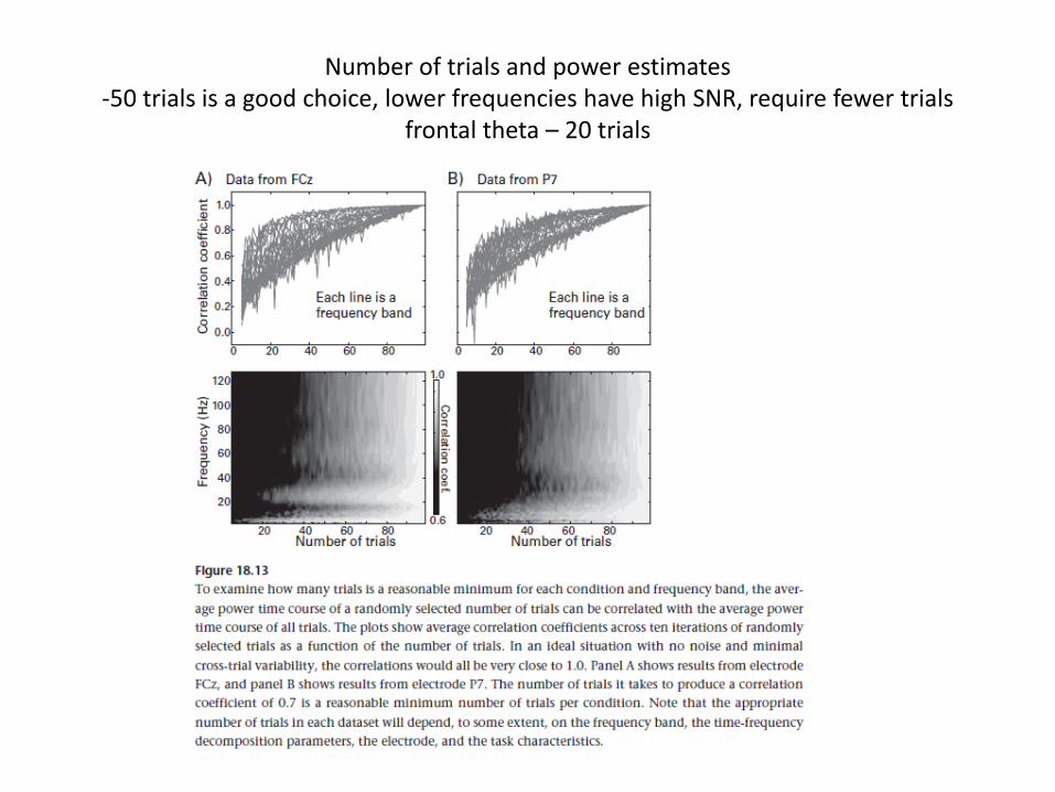
Number of trials and power estimates-50 trials is a good choice, lower frequencies have high SNR, require fewer trials

frontal theta – 20 trials

Exercises

• Select three frequency bands and compute time varying power at each electrode in these three bands, using either complex wavelet convolution or filter-Hilbert. Compute and store both the baseline-corrected power and the raw non-baseline-corrected power. You can choose which time period and baseline normalization method to use.

• 2. Select five time points and create topographical maps of power with and without baseline normalization at each selected time-frequency point. You should have time in columns andwith/without baseline normalization in rows. Use separate figures for each frequency. The color scaling should be the same for all plots over time within a frequency, but the color scaling should be different for with versus without baseline normalization and should also be different for each frequency.

• 3. Are there qualitative differences in the topographical distributions of power with compared to without baseline normalization? Are the differences more prominent in some frequency bands or at some time points? What might be causing these differences?