1

Economic evaluation of the High Speed Rail*

Ginés de Rus

University of Las Palmas de G.C. University Carlos III de Madrid

gderus@daea.ulpgc.es

Revised (May, 2012)

Abstract

Investment in high speed rail (HSR) infrastructure produces social benefits

and costs. The potential benefits are basically time savings, higher reliability,

comfort, safety and the release of capacity in the conventional rail network,

roads and airport infrastructure. The costs are high, and sunk in a significant

proportion; therefore, the social profitability of the project requires that HSR

users’ and other beneficiaries’ willingness to pay is high enough to

compensate the sunk and variable costs of maintaining and operating the line

plus any other external cost during construction and project life.

In Sweden there are now plans to build a high speed rail between the

country´s two largest cities, Stockholm and Gothenburg. The distance between

the cities is around 500 km. This is a standard medium-length line where the

HSR develops its full potential. In this paper we conduct a cost-benefit

analysis of the HSR lines for Madrid-Barcelona, Madrid-Seville and

Stockholm-Gothenburg. The first one has been running for a couple of years

and the second one since 1992, so we can evaluate their performance and

increase our understanding of the potential social profitability of similar lines,

like the Stockholm-Gothenburg where the investment decision has not been

taken so far.

* This report is undertaken for The Expert Group on Environmental Studies (Ministry

of Finance, Sweden). The author is indebted to Aday Hernández and Jorge Valido for

their work as research assistants. He is also grateful to Magnus Allgulin, Per-Olov

Johansson, Bengt Kriström, Maria Börjesson, Jean-Eric Nilsson and Bo-Lennart Nelldal

for their comments, help and support. The responsibility for opinions expressed and

for any remaining errors are solely of the author.

2

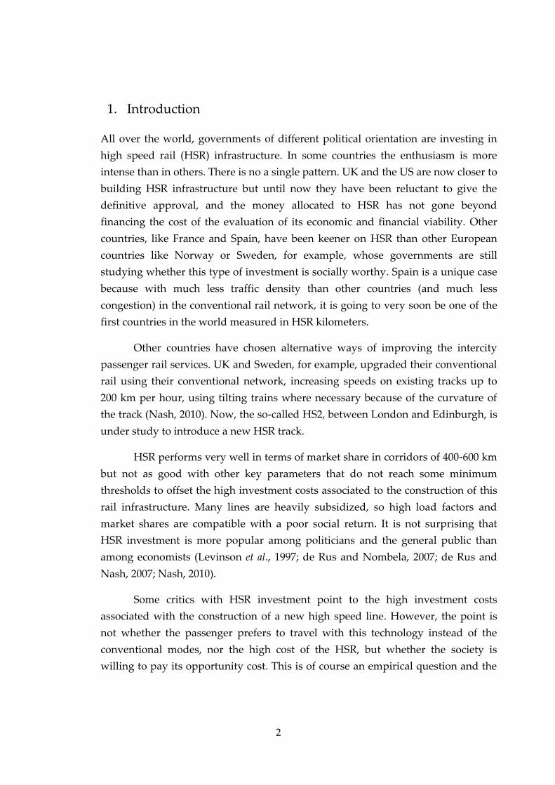
1. Introduction

All over the world, governments of different political orientation are investing in

high speed rail (HSR) infrastructure. In some countries the enthusiasm is more

intense than in others. There is no a single pattern. UK and the US are now closer to

building HSR infrastructure but until now they have been reluctant to give the

definitive approval, and the money allocated to HSR has not gone beyond

financing the cost of the evaluation of its economic and financial viability. Other

countries, like France and Spain, have been keener on HSR than other European

countries like Norway or Sweden, for example, whose governments are still

studying whether this type of investment is socially worthy. Spain is a unique case

because with much less traffic density than other countries (and much less

congestion) in the conventional rail network, it is going to very soon be one of the

first countries in the world measured in HSR kilometers.

Other countries have chosen alternative ways of improving the intercity

passenger rail services. UK and Sweden, for example, upgraded their conventional

rail using their conventional network, increasing speeds on existing tracks up to

200 km per hour, using tilting trains where necessary because of the curvature of

the track (Nash, 2010). Now, the so-called HS2, between London and Edinburgh, is

under study to introduce a new HSR track.

HSR performs very well in terms of market share in corridors of 400-600 km

but not as good with other key parameters that do not reach some minimum

thresholds to offset the high investment costs associated to the construction of this

rail infrastructure. Many lines are heavily subsidized, so high load factors and

market shares are compatible with a poor social return. It is not surprising that

HSR investment is more popular among politicians and the general public than

among economists (Levinson et al., 1997; de Rus and Nombela, 2007; de Rus and

Nash, 2007; Nash, 2010).

Some critics with HSR investment point to the high investment costs

associated with the construction of a new high speed line. However, the point is

not whether the passenger prefers to travel with this technology instead of the

conventional modes, nor the high cost of the HSR, but whether the society is

willing to pay its opportunity cost. This is of course an empirical question and the

3

answer is context specific. There is not anything intrinsically good or bad with this

railway technology and the economists do have not any other a priori position with

respect to the construction of new HSR lines, beyond the suggestion of the

importance of comparing social benefits and costs of the project under

consideration before taking any irreversible decision.

The comparison of the situation with the project with the counterfactual is

quite a challenging task. In fact, it is the comparison between two dynamic worlds.

One is the world without the project evolving with changes in income, prices and

technology, and the other is the world with the project evolving in a presumably

different way, every year during the lifespan of the project. The evaluation is based

in the comparison of each year between these two different worlds.

Investment in HSR modifies the equilibrium in intercity passenger

transport. Most of these corridors in developed countries are already in operation

and HSR projects are no more than the introduction of faster trains, changing the

generalized cost of travel with respect to the prevailing situation without project

(de Rus and Nash, 2007; de Rus, 2009).

An interesting issue related to intermodal competition in intercity corridors

is the asymmetry between the different operators. Although this is case specific, the

separation between infrastructure and services that characterizes road, bus and air

transport, puts the airlines at some disadvantage. Vertical unbundling may create

some problems for the airlines that lose the control of the service as a package. In

theory, vertical unbundling should not affect the final product supplied in the

market but, in practice, this is far from being true as travel time has a strong

component within airports, even where the airlines lose control of the process. On

the contrary, high speed railways operate as if the infrastructure and services were

integrated, controlling the access to the station and waiting time in the station. This

fact has its consequences on modal split, as access-egress, waiting time, and the

disutility of going through congested airports may determine, in the margin, user´s

choice.

The construction of a new HSR line in a particular medium distance

interurban corridor changes the modal split, and this change will occur regardless

of the social value of the HSR project. The final impact will heavily depend on the

4

pricing policy of the government with respect to the railways. The economic

evaluation of HSR investment cannot be carried out without first determining

which prices are going to be charged for HSR services. This is a key issue in

general, but decisive in the case we are evaluating, where the market shares are

very sensitive to pricing decisions taken in the public sector which affect the

playing ground for intermodal competition. The public pricing decision regarding

construction and maintenance costs of HSR infrastructure is crucial for the

competitiveness of the railway operators, the intermodal equilibrium and

eventually the result of the cost-benefit analysis of new lines. Therefore, this is an

issue that the economic evaluation of new projects should not overlook. Investment

and pricing decisions are interdependent.

There is considerable pressure on governments to built new high speed lines

as if the investment were a kind of `now or never´ decision. This does not seem to

be the case with this technology. The construction of HSR infrastructure is

irreversible and there is uncertainty associated with costs and demand. In these

conditions the question of the right moment to invest is critical as the investment

can be postponed in most cases. Hence, the optimal timing of the investment

should be addressed in the case of a positive Net Present Value (NPV). Even the

idea of `all or nothing´ is false, as it could be profitable to build a line today and

another in the future. Moreover, it is feasible to build a HSR rail track on parts of

the overall line and use it for traditional trains at the same time as it is prepared for

high speed services which would operate once demand motivates building new

tracks on missing links. There exist several `do something´ alternatives.

The purpose of this paper is basically to answer the normative question of

whether investing in the construction of HSR infrastructure in a standard medium-

distance corridor like the Stockholm-Gothenburg in Sweden is socially desirable.

The paper proceeds as follows. In Section 2, we describe the construction and

maintenance costs of HSR, discussing the cost structure of a standard medium-

distance HSR line and highlighting the fixedness of some costs and the dependence

of the variable costs with the volume of passenger-trips. This is followed in Section

3 by a discussion of the economic benefits of HSR. We analyze the main direct and

indirect benefits of a new HSR line, discussing which benefits we should

concentrate our attention on, and which others are not expected to be relevant in

answering the question of whether the investment is socially desirable.

5

In Section 4 we present the basic model for the economic evaluation of three

HSR lines. The purpose of this section is to discuss the cost-benefit analysis

framework with the aim of making our assumptions explicit, as well as to discuss

the limitations of the practical approach that we follow in Sections 5 to 7. These

sections contain an ex-post (or in medias res to be more precise) cost-benefit analysis

of two similar lines in Spain: the Madrid-Seville, in operation since 1992, and the

Madrid-Barcelona, fully in service since 2008 though operating between Madrid

and Zaragoza since 2003. Sections 5 to 7 also contain an ex ante cost-benefit analysis

of the Stockholm-Gothenburg project. Section 8 addresses the problem of

intermodal competition, pricing and its consequences on project evaluation.

Finally, conclusions are drawn in Section 9.

2. The cost of a High Speed Rail line

HSR lines have been conceived as a separate business by railway operators in

many countries. The provision of HSR services in France or Spain, for example, is

considered a different mode of transport, a new network with dedicated

infrastructure and a more specialized and technologically advanced rolling stock. It

brings with it an improvement over traditional rail transport (reliable timetables,

sophisticated information and reservation systems, catering, on board and station

information technologies services). In the case of Spain, the HSR lines are

constructed with the European gauge, narrower than the 10.000 km of the

conventional rail network.1

Both conventional and high speed railways are based on the same basic

engineering principle: rails provide a very smooth and hard surface on which the

wheels of the trains may roll with a minimum of friction and energy consumption.

Nevertheless, there are technical differences. For example, from an operational

point of view, their signaling systems are completely different: whereas traffic on

conventional tracks is still controlled by external (electronic) signals together with

automated signaling systems, the communication between a running HSR train and

the different blocks of tracks is usually fully in-cab integrated, which removes the

1 This section is based on Campos and de Rus (2009) and de Rus (2009, 2010).

6

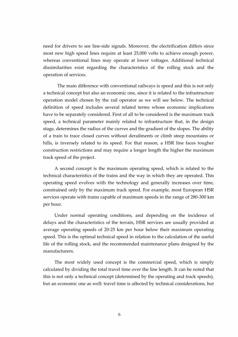
need for drivers to see line-side signals. Moreover, the electrification differs since

most new high speed lines require at least 25,000 volts to achieve enough power,

whereas conventional lines may operate at lower voltages. Additional technical

dissimilarities exist regarding the characteristics of the rolling stock and the

operation of services.

The main difference with conventional railways is speed and this is not only

a technical concept but also an economic one, since it is related to the infrastructure

operation model chosen by the rail operator as we will see below. The technical

definition of speed includes several related terms whose economic implications

have to be separately considered. First of all to be considered is the maximum track

speed, a technical parameter mainly related to infrastructure that, in the design

stage, determines the radius of the curves and the gradient of the slopes. The ability

of a train to trace closed curves without derailments or climb steep mountains or

hills, is inversely related to its speed. For that reason, a HSR line faces tougher

construction restrictions and may require a longer length the higher the maximum

track speed of the project.

A second concept is the maximum operating speed, which is related to the

technical characteristics of the trains and the way in which they are operated. This

operating speed evolves with the technology and generally increases over time,

constrained only by the maximum track speed. For example, most European HSR

services operate with trains capable of maximum speeds in the range of 280-300 km

per hour.

Under normal operating conditions, and depending on the incidence of

delays and the characteristics of the terrain, HSR services are usually provided at

average operating speeds of 20-25 km per hour below their maximum operating

speed. This is the optimal technical speed in relation to the calculation of the useful

life of the rolling stock, and the recommended maintenance plans designed by the

manufacturers.

The most widely used concept is the commercial speed, which is simply

calculated by dividing the total travel time over the line length. It can be noted that

this is not only a technical concept (determined by the operating and track speeds),

but an economic one as well: travel time is affected by technical considerations, but

7

also by other (non-technical) elements, such as the commercial schedule, the

number of intermediate stops, the quality assured to customers, etc.

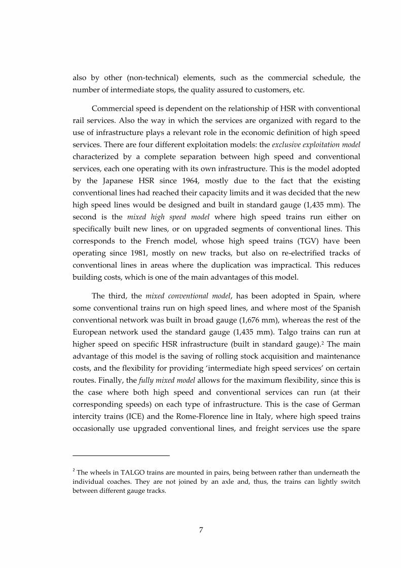
Commercial speed is dependent on the relationship of HSR with conventional

rail services. Also the way in which the services are organized with regard to the

use of infrastructure plays a relevant role in the economic definition of high speed

services. There are four different exploitation models: the exclusive exploitation model

characterized by a complete separation between high speed and conventional

services, each one operating with its own infrastructure. This is the model adopted

by the Japanese HSR since 1964, mostly due to the fact that the existing

conventional lines had reached their capacity limits and it was decided that the new

high speed lines would be designed and built in standard gauge (1,435 mm). The

second is the mixed high speed model where high speed trains run either on

specifically built new lines, or on upgraded segments of conventional lines. This

corresponds to the French model, whose high speed trains (TGV) have been

operating since 1981, mostly on new tracks, but also on re-electrified tracks of

conventional lines in areas where the duplication was impractical. This reduces

building costs, which is one of the main advantages of this model.

The third, the mixed conventional model, has been adopted in Spain, where

some conventional trains run on high speed lines, and where most of the Spanish

conventional network was built in broad gauge (1,676 mm), whereas the rest of the

European network used the standard gauge (1,435 mm). Talgo trains can run at

higher speed on specific HSR infrastructure (built in standard gauge).2 The main

advantage of this model is the saving of rolling stock acquisition and maintenance

costs, and the flexibility for providing ‘intermediate high speed services’ on certain

routes. Finally, the fully mixed model allows for the maximum flexibility, since this is

the case where both high speed and conventional services can run (at their

corresponding speeds) on each type of infrastructure. This is the case of German

intercity trains (ICE) and the Rome-Florence line in Italy, where high speed trains

occasionally use upgraded conventional lines, and freight services use the spare

2 The wheels in TALGO trains are mounted in pairs, being between rather than underneath the

individual coaches. They are not joined by an axle and, thus, the trains can lightly switch

between different gauge tracks.

8

capacity of high speed lines during the night. The price for this wider use of the

infrastructure is the significant increase in maintenance costs.

The choice of one exploitation model is a decision that affects the construction

and maintenance costs of the HSR infrastructure and the costs of upgrading (and

maintaining) the conventional network, and hence the definition of high speed

becomes not only a technical question but also an economic one. The exclusive

exploitation and the mixed high speed models, for example, allow a more intensive

usage of HSR infrastructure, whereas the other models must take into account that

(with the exception of multiple-track sections of the line) slower trains occupy a

larger number of slots during more time and reduce the possibilities for providing

HSR services. Since trains of significantly different speeds cause massive decreases

of line capacity, fully mixed-traffic lines are usually reserved for high speed

passenger trains during the daytime, while freight trains operate at night.

The cost of building and operating a HSR line consists of the construction and

maintenance of the infrastructure, the acquisition, operation and maintenance of

the rolling stock and the external costs. Sometimes, user costs are added to the total

social costs of transport. These costs are mainly related to door-to-door travel costs,

excluding money costs and including access, egress, waiting and in-vehicle time,

reliability, probability of accident and comfort. As HSR investment usually means a

reduction of the user costs, they are treated as benefits in Section 3.

The construction of HSR infrastructure requires a specific design aimed at the

elimination of all those technical restrictions that may limit the commercial speed

below 250-300 km/h. These basically include roadway-level crossings, frequent

stops or sharp curves unfitted for higher speeds so that, in some cases, new

signaling mechanisms and more powerful electrification systems may be needed, as

well as junctions and exclusive track ways in order not to share the right-of-way

with freight or slower passenger trains, when there is joint use of the infrastructure.

These common design features do not imply that all HSR projects are

similarly built. Just the opposite; the comparison of construction costs between

different HSR projects is difficult since the technical solutions adopted in each case

to implement these features differ widely. The construction (and planning) period

involves much more than track building. It requires the design and building of

9

depots, maintenance and other sites, as well as hiring and training of personnel,

testing of the material and many other preparation issues.

Infrastructure costs include investments in construction and maintenance of

the tracks including the sidings along the line, terminals and stations at the ends of

the line and along the line, respectively, energy supplying and line signaling

systems, train controlling and traffic management systems and equipment, etc.

Construction costs are incurred prior to starting commercial operations (except in

the case of line extensions or upgrades of the existing network). Infrastructure

maintenance and operating costs include the costs of labor, energy and other

materials consumed by the maintenance and operation of the tracks, terminals,

stations, energy supplying and signaling systems, as well as traffic management

and safety systems. Some of these costs are fixed, and depend on operations

routinely performed in accordance with technical and safety standards. In other

cases, as in the maintenance of tracks, the cost is affected by the traffic intensity.

Similarly, the cost of maintaining electric traction installations depends on the

number of trains running during operation.

From the actual construction costs (planning and land costs, and main stations

excluded), of 45 HSR lines in service, or under construction, the average cost per

km of a HSR line ranges from €10 to €40 million with an average of €20 million. The

upper values are associated with difficult terrain conditions and crossing of high

density urban areas (Campos and de Rus, 2009) but there are projects like the HS2

in UK with an estimated cost per km of €70 million. Infrastructure maintenance

costs are around €100,000 (2009) per km. Hence, the fixed costs of a representative

500 km HSR line are €10 billion (planning, land costs and stations excluded); and

€50 million per year for the maintenance costs of the line.

Railway infrastructure also requires the construction of stations. Although

sometimes it is considered that the costs of building rail stations, which are usually

singular buildings with expensive architectonic design, are above the minimum

required for technical operation, these costs are part of the system and the

associated services provided affect the generalized cost of travel (e.g., quality of

service in the stations reduces the disutility of waiting time). To these fixed costs we

have to add the acquisition costs of the rolling stock and the operating and

maintenance costs of running the trains.

10

Rolling stock costs include three main subcategories: acquisition, operation

and maintenance. With regard to the first one, the price of a HSR trainset is

determined by its technical specifications, one of whose main factors is the capacity

(number of seats). However, there are other factors that can affect the final price,

such as the contractual relationship between the manufacturer and the rail

operator, the delivery and payment conditions, the specific internal configuration

demanded by the operator, etc. With respect to the operating costs, these mainly

include the costs of labor and energy. These costs usually depend on the number of

trains operated on a particular line, which in turn, are indirectly determined by the

demand. Since the technical requirements (for example, crew members) of the

trains may differ with their size, sometimes it is preferable to estimate these costs as

dependent on the number of seats or seats-km. In the case of the cost of maintaining

rolling stock (including again labor, materials and spare parts), costs are also

indirectly affected by the demand (through the fleet size), but mainly by the train

usage, which can be approximated by the total distance covered every year by each

train.

There are other costs involved in a HSR project. For example, planning costs

are associated with the technical and economic feasibility studies carried out before

construction. These fixed costs, as well as those associated with the legal

preparation of the land (expropriation or acquisition from current landowners), are

not usually included in the published construction cost per km. There are other

costs difficult to allocate to infrastructure or operation, as general administration,

marketing, internal training, etc.

The operating costs of HSR services (train operations, maintenance of rolling

stock and equipment, energy, and sales and administration) vary across rail

operators depending on traffic volumes and the specific technology used by the

trains. In the case of Europe, almost each country has developed its own

technological specificities: each train has different technical characteristics in terms

of length, composition, seats, weight, power, traction, tilting features, etc. The

estimated acquisition cost of rolling stock per seat goes from €33,000 to €65,000

(2002). The operating and maintenance costs vary considerably. Adding operating

and maintenance costs and taking into account that a train runs from 300,000 to

500,000 km per year, and that the number of seats per train goes from 330 to 630,

11

the cost per seat-km can be as high as twice as it is in different countries (de Rus et

al., 2009).

External costs

It has been argued that one of the reasons supporting the case for investing in HSR

infrastructure is the positive net environmental effect associated with the operation

of HSR services once the substitution effects are included. HSR trains attract

passengers from road and air with higher environmental externalities and, when

the deviation of traffic is substantial, as it happens to be in medium-distance

corridors, the net effect on the environment of investing in HSR is likely to be

positive. Although the above argument is empirical, it helps to identify the direct

and indirect environmental effects of the HSR and whether, under reasonable

assumptions, a reduction of the environmental damage can be expected with

respect to the situation without project.

The environmental externalities of HSR point in two directions. One is

positive, due to its substitution effect on air and road traffic. In such cases, its

contribution to the reduction of these negative externalities is positive, although it

requires a significant deviation of passengers from these modes as well as high load

factors in the HSR to offset the pollution associated with the production of electric

power consumed by high speed trains.

The other is negative: High speed lines need land, crossing areas of

environmental value. The rail track creates a barrier effect in the affected territory,

produces noise and generates visual intrusion on the landscape. The net

environmental impact will depend on the reduction of environmental externalities

in other modes of transport that lose traffic in favor of the new mode. Moreover, the

emission of greenhouse gases during the construction period is massive and it may

take decades of HSR operation to compensate for the emissions caused by

construction (Kageson, 2009). The net balance of these effects depends on the value

of the affected areas, the number people affected, the benefits from diverted traffic

and so on. The net impact is very difficult to assess without contemplating the

circumstances in a particular corridor.

12

There are some facts that can help to understand the reason why this external

benefit of the HSR has been found insignificant in any independent economic

evaluation of the construction of new lines:

The environmental impact of a new HSR is not limited to the operation of

trains during the life of the project (negative or positive) but also to the

externalities during the construction period (negative). While the

environmental costs of building the line are relatively easy to quantify, those

associated to the operation are subject to a wide variability depending on the

volume and composition of traffic, load factors, etc.

There are several environmental effects of building a new line: land use,

barrier effect, noise, pollution, etc. Some of these effects (barrier effect,

negative landscape and biodiversity impacts) may be more important than

the effect on global warming but as the social debate is concentrated on this

particular effect at the moment, further research is required on these

externalities given its irreversibility.

The net effect on global warming depends on the change in the modal split

within the corridor, the generation of traffic, the load factors in the different

modes of transport, the technological change during the lifespan of the

project and the indirect effects in other markets. The reported net

environmental impact of HSR is very sensitive to the assumptions regarding

these key factors.

To the extent that infrastructure charges on road and air do not cover the

marginal social cost of the traffic concerned, there will be benefits from such

diversion. Estimation of these benefits requires valuation of marginal costs

of noise, air pollution, global warming and other external costs and their

comparison with taxes and charges

Any measurement of the expected environmental impact of a new HSR line

requires a counterfactual. The result of any cost-benefit analysis is strongly

affected by the creation of the predictable world without the project. In our

case, the construction of new road and airport capacity avoided, as well as

13

the improvement in the technology of cars and aircraft during the life of the

project, or the type of pricing to be applied in each mode of transport in the

next decades, should be taken into account.

There are many negative environmental impacts when a HSR line is built

(e.g., the barrier effect) to be weighed against the expected reduction of CO2

emission when passengers shift from road and air to rail; and though some of them

can be mitigated through tunneling, the contribution toward environmental

improvements does not seem to be a strong point of HSR investment. Even in

studies quite favorable to HSR, the conclusion with respect to the benefits on the

environment is skeptical, “…since a scheme requiring such substantial new

infrastructure would inevitably have significant negative landscape, biodiversity

and heritage impacts, with relatively small benefits to air quality and noise levels”

(Atkins, 2004).

The contribution of HSR investment to the mitigation of global warming is

also very poor, or even negative, once the CO2 emission during the construction

period is accounted for. The construction of a new line produces a large amount of

pollution emitted by the production and distribution of materials and construction

processes. These would be, for example, the production and distribution of

concrete, steel and ballast required for the different structure elements (sleepers,

railway traction power structure, rails and rail vehicles) and the distribution and

construction where trucks, bulldozers, tunnel-boring machines and other

equipment operate, and also when these materials have to be removed and

replaced to keep the track in operation.

The conclusions of the advantages of HSR in terms of global warming and

other externalities do not allow supporting the investment in HSR on

environmental grounds. Kageson (2009) calculates the effects on emissions of the

introduction of HSR in a medium-distance corridor (500 km). A deviation of

passenger-trips of 20 per cent from aviation, 20 per cent from cars, 5 per cent from

long-distance coaches, and 30 per cent from conventional trains is assumed.

Generated traffic accounts for the rest. In this 500 km corridor the HSR investment

would result in a net reduction of CO2 emissions of about 90,000 tons per year.

Assuming a volume of demand of 10 million passenger-trips per year and a price of

14

$40 per ton of CO2, the benefit of the reduction is equal to $3.6 million. As Kageson

remarked, this amount is really low in the context of HSR costs. “The sensitivity

analysis shows that alternative assumptions do not significantly change the

outcome. One may also have to consider the impact on climate change from

building the new line. Construction emissions for a line of this length may amount

to several million tons of CO2.” (Kageson, 2009).

The following study was undertaken by Booz Allen Hamilton (2007) for the

UK Department of Transport within the economic evaluation of the so-called HS2,

and it includes the emission of greenhouse gases during the construction period.

The report examines the effects on global warming of the construction of two lines:

London-Birmingham and London-Scotland. The different length of the lines is a

quite interesting fact for understanding the effects of HSR investment on the

mitigation of emissions as in the first one (500 km) rail, it is more competitive than

air but the room for additional benefits is lower, as conventional rail already had a

significant market share, so the emission during construction was a heavy burden

to offset during the change in the modal split. The second, longer line has

potentially more to gain because the market share of air is higher, but the longer

distance makes competition with air transport more difficult.

In this report, the net effect on CO2 emission of the new line is estimated

calculating the change in the emissions through the HSR line construction and

operation in order to compare it to the situation without the project. To achieve a

net reduction in carbon emissions, a reduction of the activity (traffic diversion) in

the alternative modes is required so that the carbon saved on road and air exceeds

the additional emission from the construction and operation of the HSR. The

situation where the savings in the conventional modes compensates the emission

produced by the HSR is called emissions parity.3 Therefore an estimation of the

change in the modal split in the corridor is needed to estimate whether the

deviation of demand from competing modes is enough to achieve emissions parity.

3 Emissions parity means that the amount of CO2 is similar with project and without project.

Carbon neutral means that the changes through modal split compensate the emission during

construction and operation to a level at which there are zero net emissions with the project

15

Booz Allen Hamilton (2007) circumvents the forecast of the deviation of traffic

from conventional modes to HSR estimating the required modal shifts to achieve

emissions parity. When the modal split is greater than that corresponding to

emissions parity level, the investment in HSR contributes to the mitigation of global

warming. The carbon dioxide emissions, including those from rail and air are

estimated over a 60-year period of analysis (2010-2070). Key assumptions

underpinning the analysis include the future service pattern on the new and

existing lines, and future growth in demand for rail and air. The effect of

technological improvements in the fuel efficiency of vehicles and the expected

reduction of carbon content of transport fuels are also included.

The results for the London-Manchester line show that even with a HSR

market share of 100% (54% at present) it is not possible to achieve the emissions

parity. “Therefore, based on the assumptions applied, there is no potential carbon

benefit in building a new line on the London to Manchester route over the 60 year

appraisal period. In essence, the additional carbon emitted by building and

operating a new rail route is larger than the entire quantity of carbon emitted by the

air services” (Booz Allen Hamilton, 2007).

In the case of the London to Glasgow/Edinburgh corridor, the construction of

the HSR line can reach the emission parity if rail goes from its 14% present market

share to more than 62%. This is not easy as the quality and speed of the

conventional railways are already reasonable and the distance makes it more

difficult for rail to compete with air services.

Finally, the contribution of the HSR investment to a reduction of emissions to

mitigate global warming cannot be expected to be significant even if rail market

share reaches the maximum level in the London to Glasgow/Edinburgh. “The

transport emissions account for some 23% of the 554 million tonnes of CO2 emitted

by the UK (2005 figures). However, it should be made clear that the current

emissions from rail and domestic aviation together account for only around 1% of

total UK CO2 emissions. While this does not take into account the alleged amplified

climate change effect of releasing GHGs at altitude for aviation emissions, it does

demonstrate the relative size of the opportunity for reducing emissions with a new

domestic rail line, in the context of the national carbon footprint” (Booz Allen

Hamilton, 2007).

16

The evidence for the US is similar to the one described above. Kosinski et al.

(2010) show that building a high speed network can go beyond the emission parity

making a contribution to the mitigation of carbon dioxide emissions. The HSR

system evaluated in this study includes the city pairs linked as part of the network

of the Federal Railroad Administration designated HSR corridors, and according to

their estimation, 18.0% and 28.5% of 2008 air and auto travel, respectively, were

found to be in the HSR range.

Although they show that under reasonable assumptions the investment on

HSR can make a contribution to carbon dioxide reductions, the magnitude is again

unsatisfactory from the perspective of investing in HSR for environmental reasons.

Excluding the environmental impact during construction, Kosinski et al. (2010)

conclude that HSR investment would likely lead to a modest reduction in CO2

emissions of between 0.5% and 1.1% in the passenger transport sector.

The low potential to reduce CO2 emissions in the transportation sector

compared with the original projections without HSR is primarily due to the small

share of overall travel that is between major metro regions connected within the

proposed HSR network and expected to shift from air and road to HSR.

In the case of noise, the modal comparison is less brilliant although still very

favorable to HSR. Railways noise mostly depends on the technology in use but, in

general, high speed trains generate noise as wheel-rail noise and aerodynamic

noise. It is a short-time event, proportional to speed, which burdens during the time

when a train passes. This noise is usually measured in dB(A) scale (decibels).

Measurements have been made for noise levels of different high speed train

technologies, and the values obtained ranged from 80 to 90 dB(A), which are

disturbing enough, particularly in urban areas. Levinson et al. (1997) found that in

order to maintain a (tolerable) 55dB(A) background noise level at 280 km/h, it has

been found that one needs about a 150-meter corridor between the tracks and any

other structure.

This final distance is important because it has been generally omitted in the

traditional comparisons of land occupancy between HSR and, for example, a

motorway. As a consequence, general complaints about the noise of TGVs passing

17

near towns and villages in France have led to acoustic fencing being built along

large sections of tracks to reduce the disturbance to residents.

The discussion on the environmental costs of the HSR has an interesting

dimension in Sweden. In UK, for example, the NPV of the construction and

operation of the HS2 is positive but the net balance of the environmental costs of

the project is not considered as an additional benefit of the project (Atkins, 2004). In

contrast, the Stockholm-Gothenburg-Malmo HSR lines are expected to be negative

in some studies but the contribution to the mitigation of global warming through

traffic deviation from more environmental damaging transport modes is high

enough, according to some studies, to justify the investment (Äkerman, 2011;

Janson et al., 2010). Although other studies (Nilsson and Pyddoke, 2009; Kageson,

2009; Kageson and Westin, 2010) are less optimistic, the point is that the

environmental effect is a key issue in the debate of the social worthiness of

constructing HSR lines between Stockholm and Gothenburg and Malmo. In Section

7, where the economic evaluation of the HSR in Sweden is carried out, we have a

more detailed discussion of this debate.

With respect to safety, any comparison of accident statistics for the different

transport modes immediately confirms that HSR is – together with air transport –

the safest mode in terms of fatalities per passenger-kilometers. This is so because

high speed rail systems are designed to reduce the possibility of accidents. Routes

are entirely grade-separated and have other built-in safety features. Part of safety

costs is thus capitalized into higher construction and maintenance costs, rather than

being realized in accidents. In the case of the barrier effects, alteration of landscapes

and visual intrusion, some of these external costs are also internalized in land

movements and construction, though the external part of this cost may be

overwhelming.

3. The benefits of High Speed Rail

The provision of high speed rail services in medium-distance intercity corridors

dramatically increases the market share of railways. Although society may not have

improved, some individuals are better off with the project. Some users have

18

voluntarily chosen to shift mode, having had the possibility of choosing between

the former alternative and the new one. It is true that when conventional rail

services are closed following the introduction of HSR services, some rail users do

not have a similar alternative; but at least with respect to car, bus and air, the

individual improvement is clear when the users shift from these modes to HSR.

The choice is based on the generalized cost of travel (money cost, door-to-

door travel time multiplied by the value of time of passengers; values that vary

with the level of comfort, and some other unobservable variables). The door-to-

door travel time has several components and the value passengers place on each

one is far from being the same. Passengers give more weight to access-egress and

waiting time than to in-vehicle time and this has important consequences in terms

of market shares. According to Wardman (2004) saving waiting time is valued on

average 1.5 times than in-vehicle time, and 2 times in the case of access-egress. Price

is also an important component of the generalized cost. The results of some

customer surveys may lead us to think that time is what matters for a modal split,

and that price is irrelevant, but another interpretation is that at the present level of

HSR prices, time is the key factor. Intermodal competition may thus be strongly

affected.

This individual decision between travel options is affected by the competitive

advantage of each mode of transport. The advantage can be technological, affecting

the trip length or the quality of travel, but it is also explained by the pricing policy

of the government. The market shares in medium-distance corridors are sometimes

determined in the margin by decisions taken outside of market discipline. For

example, the rail market share will vary drastically depending on whether the

infrastructure charges follow short-run marginal cost or aim for full cost recovery.

Leaving aside income transfers and focusing on the real resource changes,

HSR generates social benefits, basically time savings, higher reliability, comfort and

safety, and the reduction of congestion and accidents from alternative modes.

When users shift to HSR from buses, cars or airlines, some avoidable costs add to

total benefits. These cost savings may be significant when the equipment, energy

and labor have alternative uses.

19

Table 1 shows the direct and indirect benefits associated with the investment

in transport infrastructure. In the case of HSR, some of them are indisputable, as

happens to be the case with time savings and new users’ willingness to pay, but

others are less clear, such as the spatial effects (tunnel effect of HSR in contrast with

the corridor effect of conventional rail) or the agglomeration benefits, more

connected with urban and commuting services than with the medium-distance

intercity transport. Let us discuss the list of potential benefits in more detail.4

Table 1. Benefits of transport investment

Transport market

(derived demand)

Primary markets

(using transport) Secondary markets

Time savings Effects already measured

in the transport market

(except leisure and

commuting time savings)

Complement and substitutes

in markets with distortions

(indirect effects- intermodal

effects)

- Taxes

- Subsidies

- Externalities

- Unemployment

- Market power

Higher reliability

Higher frequencies

Wider economic benefits

- Agglomeration

- Higher competition

Reduction in

operating costs

Generated demand

Reduction of

accidents

Spatial effects and

regional development

Environmental

impacts

4 The description of the benefits is based on de Rus (2008, 2010).

20

Direct benefits measured with the derived demand for transport

The direct benefits of HSR investment come from existing passenger-trips using

conventional railway services in the corridor, the deviated demand from other

transport modes and the induced passenger-trips after the reduction of the

generalized cost of travel. The door-to door user time invested in a trip includes

access and egress time, waiting time and in-vehicle time. The total user time

savings will depend on the conditions in the initial transport mode. In the case of

conventional railway, some case studies on HSR development in seven countries

show that when the conventional rail has an operating speed of 130 km/h,

representative of many railway lines in Europe, the introduction of HSR services

yields 45-50 minutes savings for distances in the range of 350-400 km. When the

trains run at 100 km/h, potential time savings are one hour or more, but when the

operating speed is 160 km, time saving is around half an hour over a distance of 450

km (Steer Davies Gleave, 2004). Access, egress and waiting time are practically the

same in conventional and HSR services.

The case of road transport is quite different with access-egress and waiting

time, playing a decisive role in the generalized costs and eventually in modal

choice. In the case of a HSR line with 500 km length, car passengers shifting to HSR

benefit from travel time savings but they lose with respect to access, egress and

waiting time. Benefits are higher than costs when travel distance is long enough, as

HSR runs, on average, twice as fast as the average car. As the travel distance gets

shorter the advantage of the HSR diminishes as in-vehicle time loses weight with

respect to access, egress and waiting time. Nevertheless, in choosing between car

and HSR, a key factor could be whether the traveler will need a car at his

destination. This, in turn, could depend on trip purpose and the availability of mass

transit at the destination. Similarly, the number of people traveling together could

matter as the marginal cost of a second person traveling in a car that is already

making the trip is near zero. Moreover, it is usually assumed that trip quality is

higher for HSR than for auto travel. In some ways, that may be true, but not in all

ways. For example, one can stop when and where one likes and it is easier to carry

luggage with oneself if traveling by car (de Rus, 2010).

In the case of air transport the picture is also different. In-vehicle time is

longer by train but it is assumed that the user saves access, egress and waiting time,

21

and enjoys additional service quality. The evidence (Wardman, 2004) is that the

money value of time of access-egress and waiting time are of the order of 2 and 1.5

times higher, respectively, than in-vehicle time and hence, even in the case of

longer door-to-door travel time after the shift, the value of time savings of a

passenger shifting from air to rail could be positive, as far as the values of time of

access-egress and waiting time are high enough to compensate the losses in-vehicle

time. Nevertheless, the condition of a lower access and egress time for HSR than for

air travel not always holds. Clearly, it depends on the exact origin and destination

of the trip. Particularly for non-business travel, but even for business travel to

suburban locations, air travel might have an advantage in access and egress time as

well as in line-haul time.

The relative advantage of HSR with respect to air transport is significantly

affected by the existing differences in the values of time, and these values are not

unconnected with the actual experience of waiting, queuing and passing through

security-control points in airports. Hence, one should not discard the implications

of more demanding security measures for rail travel. If these measures are taken,

demand for HSR relative to other modes could decrease for two reasons: trip time

could increase and trip quality could decrease.

It is worth stressing that under these circumstances the market rail share,

crucial for the success of HSR investment, depends on some conditions to be

fulfilled. The main condition to be fulfilled is that the generalized cost, net of

transfers, be lower. This means that the resource cost is lower when the passenger

shifts to HSR, but this may happen even in the case of negative net door-to-door

travel time benefits if the avoidable resource cost in the initial mode of transport is

high enough to offset those losses. It seems clear at this point that the magnitude of

the total net benefits of passengers shifting modes are very sensitive to a set of

variables which can take values within a wide range depending on the local

conditions in the corridor. Yearly net benefits have to be significant to compensate

HSR variable costs and then to produce a surplus per year high enough to

compensate the initial investment costs.

Benefits also come from induced demand. The new passenger-trips of HSR

may come from different sources: completely new generated trips; trip

redistribution, i.e., trips that were made to a different destination without the

22

project; diverted demand from other modes of transport; and finally, route or time

reassignment. In the three first cases the number of passenger-trips increases for the

project and so we have to account for the willingness to pay of both the deviated

and the generated demand. The interesting point is that both types of demand can

be measured with the same method (Abelson and Hensher, 2001). Users who

switch to HSR from an alternative transport mode as well as new users or existing

users traveling more, have benefits that go from the total marginal change to zero.

The conventional approach for the measurement of the benefits of new

demand is to consider that the benefit of the inframarginal user is equal to the

difference in the generalized cost of travel with and without HSR. The last user

with the project is indifferent between both alternatives, so the user benefit is zero.

Assuming a linear demand function, the total user benefit of generated demand is

equal to one half of the difference in the generalized cost of travel (the `rule of a

half´).

Nevertheless, this method may be misleading when the implementation of

the transport project also affects some quality elements of the journey or there is a

change in the frequency. In the first case, the application of the `rule of a half´ may

underestimate the willingness to pay of the total benefits when using the resource

cost approach, unless the additional willingness to pay for `quality´ is included

(Abelson and Hensher, 2001). In the second case, when there is also a change of the

time between services (headway), the change in consumer surplus has to be

calculated taking into account all the transport modes, even when the schedule

changes for only one of them (Jansson et al., 2010).

Indirect, spatial and wider economic impacts

It is not uncommon to find the emphasis on the indirect effects, wider economic

impacts and regional development instead of the direct effect when a HSR project is

presented by its promoters. It is true that transport investments produce other

alleged benefits beyond the direct benefits already discussed, but it is unclear

whether these additional benefits are new ones or double counting, as shown in the

second column of Table 1. Moreover, some genuine indirect benefits exist but many

of them could be associated with any other infrastructure project in general, and

not exclusively with high speed, so even if the benefits increase the social return on

23

the investment in transport, they do not necessarily place high speed in a better

position over other options for transport investment. Moreover, in undistorted

competitive markets, theory tells us that the net benefit of marginal change in a

secondary market is zero.

The framework of conventional cost-benefit analysis does not include the

evaluation of the impact of transport infrastructure projects on regional

development. Puga (2002) argues that concentrating on the primary market and

some closely related secondary market may be justified, provided that two

conditions are met: first, that distortions and market failures are not significant and

so there is no need to worry with the indirect effects of the project; and second,

“the changes in levels of activity induced by the project fade away fairly rapidly as

we move away from those activities more closely related to it. However, these

conditions are often not met. There has been increasing realization throughout

economics that wide ranges of economic activities may be affected by market

failure and distortions. And the type of cumulative causation mechanisms modeled

by the new economic geography can make the effects of a project be amplified

rather than dampened as they spread through the economy” (Puga, 2002).

Should we worry about these wider economic benefits in the case of HSR

investment? Puga (2002), Duranton and Puga (2001) and Vickerman (1995, 2006)

suggest that additional benefits are not expected to be very important in the case of

high speed railway infrastructure. The reason is that freight transport does not

benefit from high speed and therefore the location of the industry is not going to be

affected by this type of technology. Moreover, in the case of the service industry,

HSR may lead to the concentration of economic activity in the core urban centers.

Recent research (Graham, 2007) suggests that agglomeration benefits in

sectors such as financial services may be greater than in manufacturing. This is

relevant to the urban commuting case but arguably is important for some HSR

services (e.g., the North European network which links a set of major financial

centers and may be used for a form of weekly commuting). It may be erroneous to

conclude that scale economies and agglomeration economies (productivity impacts)

are only found in manufacturing and freight transport.

Hernández (2010) examines the relationship between the construction of the

Spanish HSR network and the creation of employment in the municipalities that

24

benefit from the infrastructure. He develops an econometric model that explores

the relationship between the density of employment and the existence of the HSR

in different geographic areas. The motivation for exploring this relationship is to

check whether the provision of infrastructure generates additional benefits to those

considered in conventional cost-benefit analysis. The author uses GIS

(Geographical Information System) with areas within concentric circles of 20

kilometers around the high speed rail stations to estimate the impacts of the

infrastructure on the employment density. Given the existence of municipalities

under and out of the influence of HSR, the strategy is to compare both groups with

panel data to control the possible existence of unobservable variables. Moreover, to

avoid the possible existence of endogeneity between the provision of the

infrastructure and the increase of the employment density, the author includes a set

of instrumental variables. A matching procedure is used to avoid the irrelevant

comparison between groups under and out of the influence of HSR.

The results show that the magnitude of the impact of HSR rail is around 3.5-

1.8% on the employment density of 10-20 km concentric areas around the station,

taking into account the use of instrumental variables to solve potential problems of

endogeneity. The author interprets the results with the aim of distinguishing

between relocation effects and net effects, concluding that it is not possible to

disentangle both effects and that the existing literature has not been able to

differentiate it either.

Investment in HSR as well as other transport infrastructures has been

defended as a way to reduce regional inequalities. If the definition of personal

equity is difficult, its spatial dimension is even more elusive. European regional

funds aim to reduce regional inequalities, but the problem is to define clear

objectives so that it is possible to compare the results of different policies. The final

regional effects of infrastructure investment are not clear and depend on of the type

of the project and other conditions as wage rigidity and interregional migration.

There are some ambiguities related to the role of opposite forces which affect the

balance between agglomeration and dispersion. It is difficult a priori to predict the

final effect.

Indirect effects are the impact of HSR on secondary markets, whose

products are complements to, or substitutes for, the primary market. There are

some indirect effects of HSR which, in some cases, may be important. These effects

25

are called intermodal effects and take place in the substitutive (or complementary)

mode of transport of the HSR. Are users of the alternative modes better off with

HSR? What about the producers? It is important to distinguish here between

transfers and real resource changes. We have already seen the direct benefits that

society gains from the introduction of HSR, but users who remain attached to their

former modes of transport may be affected positively or negatively depending on

whether there are distortions on these modes of transport. The same is applicable to

other economic agents.

The critical issue is whether price is higher or lower than marginal social

cost in the alternative mode of transport. When price is below marginal cost in the

original transport mode, society benefits from the diversion of demand to the new

transport mode (assuming price equal to marginal cost in the new mode). This

could happen because of the reduction of excessive congestion, or pollution. In the

case of a positive externality the opposite might occur, and the indirect effect could

be negative when the price is above the social marginal cost in the original

transport mode, for example, if the reduction of demand in the original transport

mode forces the operators to reduce the level of service, thereby increasing the

generalized cost of travel.

The key point is whether the original transport mode was optimally priced.

Although it has been argued that the reduction of road and airport congestion is a

positive effect of HSR, this is only the case if there is a lack of optimal pricing.

When road and airport congestion charges internalize the external marginal costs,

there are no indirect benefits from the change in modal split. This can be viewed

from another perspective. The justification of HSR investment based on indirect

intermodal effects should be first compared with a “do something” approach,

consisting of the introduction of optimal pricing.

It should also be mentioned that, for example, given the impossibility of

road pricing, a second-best case for HSR investment based on indirect intermodal

effects, requires significant effects of diverted demand on the pre-existing demand

conditions in the corridor. This means the combination of significant distortions,

high demand volume in the corridor and sufficiently high cross-elasticity of

demand in the alternative mode with respect to the change in the generalized cost.

26

The assumption that price is equal to the social marginal cost means that the

loss of traffic by conventional modes of transport does not affect the utility of those

who continue to use these modes of transport, nor the welfare of producers or

workers in these modes. This would mean that operators are indifferent to losses in

patronage, or workers are indifferent when losing their jobs, because in both cases

they are receiving, in the margin, their opportunity costs. There are many reasons

to abandon this assumption, one of which is the existence of unemployment, but

we will concentrate here on how the reduction of demand in air and bus transport

affects user’s utility when the operators respond to a lower demand by reducing

the service level.

Intercity bus services operate under concession contracts in many countries

and so they cannot change their basic regulated timetables in the short run.

Although they may cut the number of bus-trips when demand diminishes, the

reduction in supply does not affect frequencies since the suppressed services leave

at the same time as approved in the basic regulated timetable. However, it can be

argued that although users are barely affected by the short-term adjustment of bus

operators, financial difficulties will emerge later in contract renegotiations or when

concessions expire. This means that users and/or taxpayers (or workers) will have

to pay for the adjustment in the medium-term.

Airlines operate in open competition and therefore the short-term

adjustment in response to the external shock in demand produced by the

introduction of HSR services is the observed reduction in the number of operations.

This affects frequencies, first because the reduction in demand is substantial;

second, because airlines are not subject to public service obligations and so the

adjustment is legally feasible; and third, because of the nature of flight operations

(slots required for take-off and landing) frequencies are necessarily affected when

services are cut. The reduction in the number of flights per hour increases total

travel time when passengers arrive randomly, or decreases utility when they

choose their flight in advance within a less attractive timetable.

Regarding the spatial effects, high speed lines tend to favor central locations,

so that if the aim is to regenerate the central cities, high speed train investment

could be beneficial. However, if the depressed areas are on the periphery, the effect

can be negative. The high speed train could also allow the expansion of markets

and the exploitation of economies of scale, reducing the impact of imperfect

27

competition and encouraging the location of jobs in major urban centers where

there are external benefits of agglomeration (Venables, 2007; Graham, 2007). Any of

these effects are most likely to be present in the case of service industries

(Bonnafous, 1987). Location effects are dependent on many factors and it is difficult

to determine a priori whether the center or the periphery will be benefit from the

relocation of the economic activity (Puga, 2002).

There is evidence on the increase in land values (Cascetta et al., 2010; Preston

and Wall, 2008) or on the increase in the GDP of places where HSR stations are

located (Ahlfeldt and Feddersen, 2009). However, the problem is to disentangle

genuine additional benefits from transfers resulting from the relocation of economic

activity from other areas of the country, or from a simple reflection of the already-

measured time savings into property values (Nash, 2010). Levinson (2010) identifies

two major impacts in land values, one positive linked to accessibility benefits, and

the other negative linked to noise along the line. The author argues that the effects

on land use near the HSR stations are not significant when the traffic is not for

commuting purposes. An example is Eurostar, a HSR line connecting London and

Paris where “The development effects are not local (unlike public transit stations),

which is not surprising since if they are serving long distance travel they are also

serving less frequent travel, and as a consequence the advantages of being local to

the station are weaker” (Levinson, 2010).

In cases where the saturation of the conventional rail network requires

capacity expansions, the construction of a new high speed line has to be evaluated

as an alternative to the improvement and extension of the conventional network,

with the additional benefit of releasing capacity. Obviously the additional capacity

has value when the demand exceeds the existing capacity on the route. Under these

circumstances the additional capacity can be valuable not only because it can

absorb the growth of traffic between cities served by the HSR, but also because it

releases capacity on existing lines to meet other traffic like suburban or freight. In

the case of the airport, the additional capacity can be used to reduce congestion or

scarcity. In any case, the introduction of HSR would produce this additional

benefit.

The existence of network externalities is another alleged direct benefit of

HSR (see Adler et al., 2007). Undoubtedly, a dense HSR network offers more

possibilities to rail travelers than a less developed one. Nevertheless, we are

28

skeptical of the economic significance of this effect. We do not argue against the

idea that networks are more valuable than disjointed links. The point is that when

there are network effects, they should be treated as benefits at a route level.

Although rail passengers gain the wider origin-destination menu, the utility of a

specific traveler who is traveling from A to B in a denser network does not increase

with the number of passengers unless the frequency increases, and this effect (a sort

of Mohring effect) is captured at a line level.

4. The Cost-Benefit Analysis (CBA) framework

The economic evaluation of HSR investment

We are examining the expected welfare effect of the projected construction of a

HSR infrastructure in an intercity corridor, where people commute or travel for

business or leisure or other purposes, and where bus companies, airlines and rail

operators compete between them, and with cars, for passenger-trips. HSR services

reduce rail travel time, changing the modal split in the corridor. In situations with

capacity constraints in the conventional rail network and airports, additional

benefits may be derived from the construction of new lines through the release of

capacity for freight and other types of services in the case of rail, and for other

destinations in the case of airports.

Other things happen as traffic is diverted from road and air to rail, and the

demand shifts in many other secondary markets, with products which are

complements or substitutes of transport services. Some cities may become more

accessible and some additional economic benefits may have to be added to the

conventional direct and indirect benefits, though it is essential (but difficult) to

distinguish between genuine wider economic benefits from mere relocation of

previously existing economic activity. Even in the case of additional benefits as it is

the case of agglomeration economies, the possibility of other areas losing benefits

for the same reason should not be discarded.

The story does not end here. The resources allocated to the HSR

infrastructure and services are significant. Construction costs exceed those

corresponding to any other transport alternative, and these costs include a

29

significant environmental impact. The rest of the costs are distributed during the

life of the project: rolling stock, energy, maintenance, labor and the environmental

costs associated to the provision of services.

Moreover, investment costs are paid by the taxpayers in many cases, in a

significant proportion, as HSR is constructed, and the services provided, by the

public sector. Nevertheless, although the investment in dedicated high speed

infrastructure is an expensive option for the improvement of rail transport, the

point is not about the amount of HSR investment costs. The relevant issue is

whether the society is willing to pay for this investment. The question is whether

the social benefits of HSR investment are worth its costs. 5

Contemplating a particular corridor we would need to know the change in

welfare with the project with respect to the situation without the project and this is

far from being an easy task. Let us suppose that a new HSR project is being

considered. The first step in the economic evaluation of this project is to identify

how the investment, a `do something´ alternative, compares with the situation

without the project. A rigorous economic appraisal would compare several relevant

`do something´ alternatives with the base case. These alternatives include

upgrading the conventional infrastructure, management measures, road and

airport pricing or even the construction of new road and airport capacity. We

assume here that relevant alternatives have been properly considered.

The investment in HSR can be seen as a perturbation in the economy,

changing individuals’ utility. These changes, occurring to many individuals in

many markets and during a long period of time have different signs. Some

individuals are better off with the project and others are worse off. Leaving aside

the problem of adding gains and losses accruing to different individuals, we have a

first question to answer related to the identification of the causal effect of the

introduction of HSR.

We are looking for the change in the utility of the individual when the

project is introduced, and this requires comparing the level of utility that an

individual would have had if the project had not been implemented. Therefore, we

need to construct a counterfactual and probably this is one of the most complex

issues in the economic evaluation of projects. We have to imagine the world

5 For a general equilibrium cost-benefit rules see Johansson (1993).

30

without the project every year during the lifespan of the project and compare it to

how we think the world will evolve with the project. Then we compare these two

moving imagined pictures.

A practical approach for the economic evaluation of investing in HSR

There are two approaches to estimate the net present value of any project:

aggregating the change in the surpluses, derived from the implementation of the

project; or alternatively, ignoring transfers between different individuals, and

accounting for the changes in resource costs and willingness to pay. When adding

the surpluses of different agents, we obtain the net social surplus. In this process of

aggregation, transfers net out, and therefore we find the real gains from the project

net of costs. This is equivalent to calculating the time savings, increase in comfort,

reduction of accidents, net willingness to pay of generated passenger-trips, etc., net

of investment, maintenance and operating costs, and external costs.

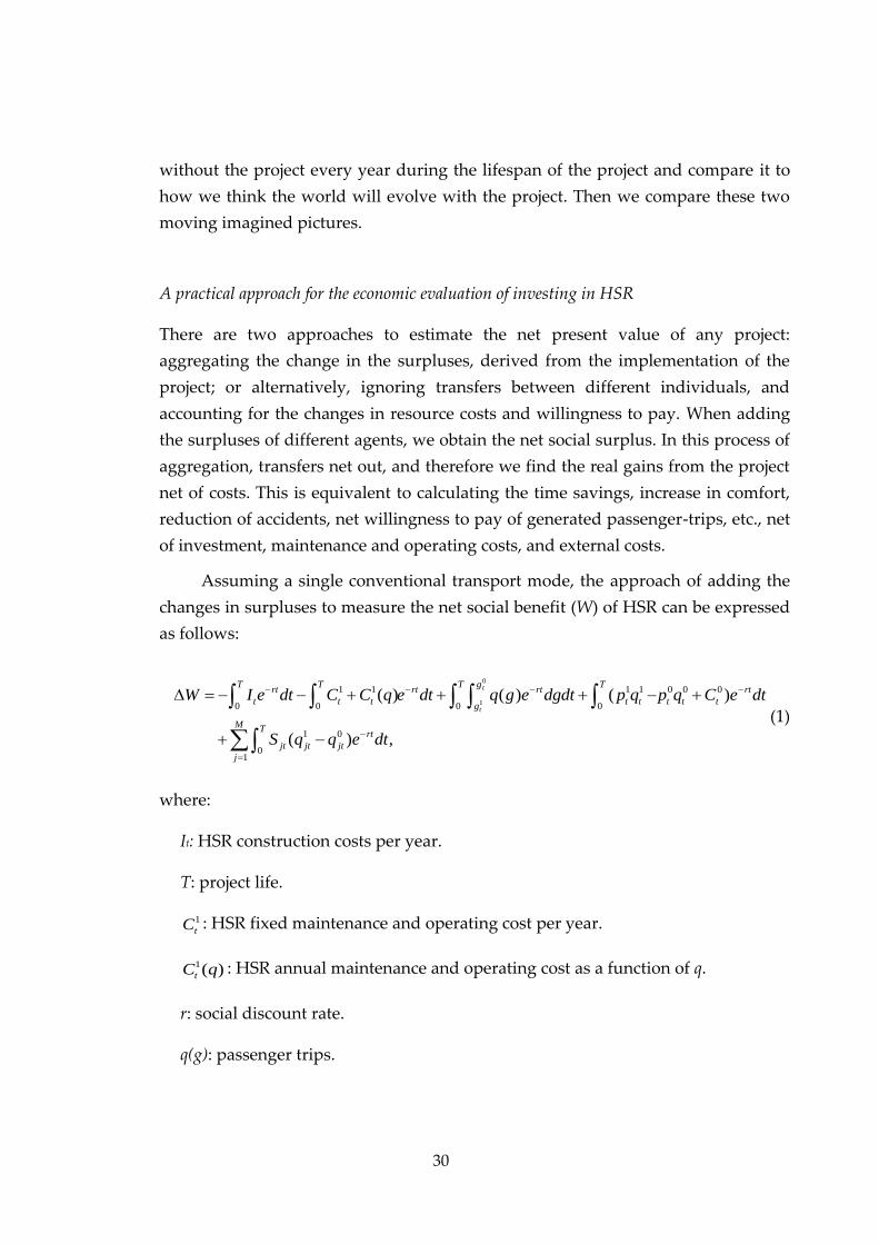
Assuming a single conventional transport mode, the approach of adding the

changes in surpluses to measure the net social benefit (W) of HSR can be expressed

as follows:

0

1

1 1 1 1 0 0 0

0 0 0 0

1 0

01

( ) ( ) ( )

( ) ,

t

t

T T T g Trt rt rt rt

t t t t t t t tg

M Trt

jt jt jt

j

W I e dt C C q e dt q g e dgdt p q p q C e dt

S q q e dt

(1)

where:

It: HSR construction costs per year.

T: project life.

1

tC : HSR fixed maintenance and operating cost per year.

1( )tC q : HSR annual maintenance and operating cost as a function of q.

r: social discount rate.

q(g): passenger trips.

31

0

tg : generalized cost without the HSR project.

1

tg : generalized cost with the HSR project.

0

tp : price without the HSR project.

1

tp : price with the HSR project.

0

tq : demand quantity without the HSR project.

1

tq : demand quantity with the HSR project.

0

tC : annual avoidable cost of the conventional mode.

M: other markets in the economy.

jtS : excess of benefits over costs in market j of a unit change in qjt.

0

jtq : level of activity in market j and year t without the project.

1

jtq : level of activity in market j and year t with the project.

We distinguish between two types of agents in (1). Those affected in the

primary market: direct users (existing, deviated and generated), producers,

individuals affected by the externalities during the construction and operation of

the project; and those affected in the secondary markets, i.e., the indirect effects in

markets with distortions (basically intermodal effects). There are other candidates

like the so-called wider economic benefits (excluded in equation (1) but discussed

in this paper).

The main benefit comes from travel-time savings. We focus mainly on the

measurement of time savings produced as a result of investing in a faster transport

mode and the individual valuation of these time savings. However, HSR users

usually include the higher reliability of HSR compared with air transport, and the

higher comfort, as additional reasons for explaining why they choose HSR instead

of other available alternative modes. A higher willingness to pay for enhanced

quality or for higher safety may be left out following the resource cost approach,

unless it is already included in the value of time.

32

It has been argued that the benefits of the time savings are underrepresented

through the value of time. There may be agglomeration benefits from infrastructure

investments due to better matching, learning and sharing. Some of the

agglomeration benefits are external, hence not captured by the values of time for

commuting (the way we estimate them), because people pay income tax.

Individuals take only into account the potential net income increase due to shorter

travel time when we measure their value of time. The proportion of the income

increase (if any) that does not go to the individual (due to taxation) is external and

should be added as a separate benefit (if unemployment decreases this part of the

benefit could be significant).

Now, some of the agglomeration effect would be external to the individual

and the company (in case of business travelers) even if there were no taxes. This is

because other companies and workers benefit from the individual’s time gain

(matching/learning/sharing). This effect is not included in values of time, for

business trips or for (private) commuting trips. To measure this part of the

agglomeration effect is truly difficult. Nevertheless, in the case of HSR investments

it seems unlikely that these additional benefits are significant due to the longer

distances compared with the evidence of agglomeration benefits in true commuting

services (Graham, 2007).

Environmental impacts are both a direct effect of the project (construction

and operation) but there may exist positive externalities such as an indirect effect

through the deviation of traffic from less environmental friendly transport modes

(accounted for in expression (1) in the last term of the equation).

For illustrative purposes (the real calculus is done with all transport modes

and as disaggregated as the data allow) let us see how the surplus approach in (1) is

equivalent to the resource-cost approach. In the case of passengers already

traveling by train, for example, without the project, the generalized cost is g0, and

the number of trips q0. The generalized cost without the project includes the

monetary component p0, the total value of travel time, and other disutility elements

related to the conventional train (g0–p0).

Under these assumptions, the social surplus is equal to users´ surplus and

producer´s surplus in the conventional train:

33

0 1 0 0 1 1 0 1 1 0 0 0 11

,2

g g q g g q q p q p q C C (2)

where 0C represents the avoidable costs of the conventional train and 1C represents

here all costs (fixed and variable) of HSR.

With the resource-cost approach the introduction of HSR generates time-

saving benefits for the existing and deviated traffic plus the additional net

willingness to pay of the generated demand.

0 1 0 0 1 1 0 1 1 0 1 1 0 0 11.

2v q g g q q g q q v q q C C (3)

It is straightforward to show that both expressions lead to the same results.

Ignoring transfers ( 0 0p q ) in (2) and given that 1 1 1g v p in (3), we get the

following expression:

0 1 0 0 1 1 0 1 1 0 0 11,

2v q g g q q p q q C C (4)

where v is the value of time and 0 and 1 the travel times, without and with the

project respectively.

Hence, the direct benefits of HSR are the money value of time savings for

existing traffic plus the additional revenue from generated (and diverted demand)

and the value of the triangle between the generalized costs. To these benefits we

have to add the change in costs (presumably negative with this technology).6

It is useful to distinguish between existing rail passenger-trips from deviated

and generated traffic. The `rule of a half´ is applicable for all types of traffic but one

should be careful when applying average time savings per passenger-trip category

when there is no existing traffic but the whole traffic is either deviated or generated as

it happens to be the case with bus, air and road passengers shifting to high speed

trains.

6 With data scarcity, or in a first approximation, it is possible to approach the benefits

represented in both expression adding the time user benefits and the revenue of new traffic.

34

Additional benefits can be obtained from intermodal readjustment. In

addition to the intermodal effect already measured in the HSR demand as a direct

benefit obtained by users of other modes of transport who become HSR users, we

have to add the effect of the reduction of traffic in the substitutive mode on the cost

of traveling for the users who remain in the conventional mode once the project is

implemented.

The existing transport modes are not the only markets affected by the

introduction of the new mode of transport. Many other markets in the economy are

affected as their products are complements or substitutes of the primary markets.

The treatment of these so called `indirect effects´ are similar for any secondary

market, be it the air transport market or the restaurants of the cities connected by

the HSR services (Harberger, 1965; Mohring, 1976). The condition for indirect

effects to be translated into additional benefits (or costs) is that some distortion in

the secondary market exists (see Table 1) and then there is a gap between the

marginal social cost and the marginal willingness to pay in the equilibrium.

The secondary intermodal effects can be positive or negative depending on

the sign of the distortion and the change in the quantity in the secondary market.

The reduction of road congestion and airport delays has been identified as an

additional benefit of the introduction of HSR. Expression (1) shows that the

existence of this benefit requires the divergence between price and marginal cost.

Where road or airport congestion charges are optimally designed, there are no

additional benefits in these markets. Even in the presence of a distortion, a

sufficiently high cross elasticity of demand with respect to the generalized cost in

the secondary market is needed to have a significant economic impact.

5. Ex-post evaluation of the HSR Madrid-Seville

Before dealing with the evaluation of the Madrid-Seville HSR line, it is worth

mentioning the scarcity of published information on costs and demand. The lack of

transparency concerning the economic profitability of HSR in Spain is remarkable.

The economic effects on the HSR lines circulated by the Spanish government have

no relation whatsoever with the economic appraisal of projects, but rather with the

type of impact studies where investment is not a cost but a benefit, including the

35

multiplier effect, labor is not an input but an output, and transfers and relocation of

economic activity are not considered, etc.

The economic evaluation of the Madrid-Seville line is based on the cost and

demand information contained in de Rus and Inglada (1993) but this is the only

common content of that original CBA and the present in media res CBA of the first

Spanish HSR line. In what follows we describe the CBA of the Madrid-Seville and

interpret the result of the density function of the net present values obtained

through a risk analysis of the project.

Madrid-Seville was the first HSR line constructed in Spain. The 471 km line

started its operation in April 1992. The investment period lasted from 1987 until

1993. Total investment was €2.1 billion (1986) and these costs were distributed

during the construction period according to the real disaggregation of these costs

per year as reported in de Rus and Inglada (1993). Investment costs are inclusive of

indirect and income taxes.7 The project is assumed to have an economic life of 50

years and for simplicity we ignore any potential residual value.8

The line allows the operation of high speed dedicated rolling stock and other

conventional trains like Talgo to provide rail services between Madrid and Seville,

Madrid-Cordoba, Cordoba-Seville and others O-D like high speed commuter

services between Madrid and Ciudad Real.

Levinson et al. (1997) provide a description of operating and maintenance

costs that is very useful for the allocation of labor cost and equipment and

materials for shadow-pricing purposes. Sales and administration costs include

labor costs for ticket sales and for providing information at the railroad stations,

automated ticketing machines and travel agency commissions. Based on data from

the French railways, the authors assumed these costs represent 10% of the

7 The reason why we have not accounted for the investment costs net of taxes is because

planning costs, land values and the construction costs of the stations and other facilities are not

included in the investment cost of the line. Even so, real investment costs might possibly be

substantially higher.

8 The main results do not change when the usual ad hoc percentages of the investment are

included at the end of the lifespan of the project.

36

passenger revenue. With the development of the new information technologies in

the last decade, one should expect a decrease of these costs.

Train operations can be divided into four activities: train servicing, driving,

operations and safety. Train operating costs consist exclusively of labor costs.

Operations and safety on either high speed or conventional lines can be estimated

on a per-train basis. The cost of the maintenance of electric traction installations

and catenary depends on the number of trains running on the infrastructure,

whereas the cost of maintaining the tracks depends on the number of train sets.

Theoretically, the cost of maintenance of equipment is dependent upon the distance

run by every train as well as the duration of use. The proportions of the cost of

labor in the maintenance costs are 55% for maintenance of electric traction

installations, 45% for maintenance of tracks and 50% for maintenance of equipment

(Levinson et al., 1997)

The maintenance cost of the infrastructure per kilometer is 100,000 €/km in

2009. From the description above, we assume half of these costs correspond to

labor and in the case of the operation and maintenance of the rolling stock, we

assume all costs are labor. Shadow pricing of labor is applied using a conversion

factor of 0.9 according to some evidence for Spain (Del Bo et al., 2009) and the other

half of infrastructure maintenance is computed net of indirect taxes. The value

added tax goes from 13% for the period 1987-1992; 16% for 1992-2010; and 18%

from 2010 onwards (see Appendix 5.1 for more detailed information). The

maintenance and operation cost per train was €2,841,774 in 1986 (de Rus and

Inglada, 1993).

For the estimation of total operating costs we need the number of trains and

the price of these trains. We assume the cost of a train follows a random uniform

distribution with a range between €33,000 and €65,000 per seat in 2002, and each

train has an average capacity of 330 seats and an economic life of 30 years (Campos

and de Rus, 2009).

We assume demand is distributed uniformly during the day (no peak hours).

The load factor follows a random uniform distribution with a minimum value of

0.6 and maximum of 0.7. The number of daily services required, given the load

factor, the length of the route and the hours of operation and a contingency factor

37

of 1.5 to allow for maintenance and other contingencies, is computed according to

Campos et al. (2009). Trains operate 16 hours per day and do not exceed the

maximum number of kilometers per year (500,000 km). The final number of trains

in the evaluation is the maximum between these two previous rules.

Other general assumptions affecting key parameters are the following: the

annual growth rate of income is taken from the National Institute of Statistics until

2009. From 2010 to 2015, the estimated growth rate is equal to 1% according to the

International Monetary Fund (IMF). For the rest of the evaluation period, the

annual growth rate follows a random uniform variable between 1% and 4%,

independent between years. The net present value is calculated at the beginning of

1987, with benefits and costs expressed in €1986. Prices are deflated with the CPI of

the National Institute of Statistics. The social discount rate of the base case is 5%

and the shadow multiplier of public funds is 1.

Demand is based on real data for the period 1992-2004, while for the rest of

the project life we have projected the number of passenger-trips of previous years,

assuming that the demand-income elasticity is equal to 1. In 1993, the first full year

of operation, 2.8 million passenger-trips were transported in the whole line: 1.2

million between Madrid and Seville and 0.9 as commuter services between Madrid

and Ciudad Real and other short distance O-D.

The estimation of the diverted traffic from the different modes per O-D and

year is based on the demand of that year in the route multiplied by the percentage

of the diverted traffic based on COST318 (1998). Passenger-trips completing the

whole length of the line (Madrid-Seville) were initially air transport users (45%),

bus users (2%), conventional train users (26%), car users (12%) and the rest (15%)

corresponds to new trips that were not made previously on any transport mode.

In-vehicle time is around 2.5 hours and this is a substantial reduction with

respect to conventional rail and road transport. On the contrary, air transport has a

substantially lower flying time (approximately one hour). Modal split and the

estimation of user benefits require going from in-vehicle time to door-to-door

travel time and then, adding the money cost, to the generalized cost of travel. Let

us have a closer look to the main long-distance O-D, Madrid-Seville and one of the

short-distance O-D, Cordoba-Seville.

38

Figure 1. Door-to-door trip time (Madrid-Seville)

0

1

2

3

4

5

6

7

8

HSR Plane Bus Car Conventional

Train

Ho

urs

Access and Egress Waiting In-vehicle

According to Figure 1 the faster way to travel between Madrid and Seville is

by air. Door-to-door travel time is shorter, though the comparative advantage rests

on the substantially shorter in-vehicle time as the access-egress and waiting time

are higher when the airport infrastructure is involved. This is quite interesting

because the higher values of access-egress and waiting time leave HSR in a better

position when door-to door travel-time costs is the reference (Figure 2).

39

Figure 2. Time-saving benefits per passenger-trip (Madrid-Seville)

0

20

40

60

80

100

120

140

160

180

Plane HSR Bus HSR Car HSR CT HSR

Plane Bus Car Conventional Train

Eu

ros

2010

Access and Egress Waiting In-vehicle

Figure 2 shows that average time benefits from deviated demand are mainly

concentrated in passengers already using railways. The average time benefit is also

high for passengers shifting from buses but is not relevant in absolute terms given

the number of bus users. The money value per passenger-trip shifting from air

transport is quite small and 45% of total demand comes from this mode of

transport. However, individual modal choice is not based on resource costs but on

the generalized cost of travel; i.e., door-to-door trip time multiplied by the value of

time of passengers plus the money cost. Figure 3 is illustrative of the strong modal

competition in this O-D.

40

Figure 3. Generalized cost per passenger-trip (Madrid-Seville)

0

50

100

150

200

250

Plane HSR Bus HSR Car HSR CT HSR

Plane Bus Car Conventional Train

Eu

ros

2010

Time component Price

The average generalized cost of HSR is quite close for air transport and car

users. Only 12% of total passenger-trips were initially car users. It is worth pointing

out that the similarity of the generalized costs of air, car and HSR is conditioned on

the pricing policy of the government with respect to HSR infrastructure and, in the

case of air transport, with the prevailing conditions in airports.

Cordoba-Seville, a representative O-D of other short-distance trips, shows

the competitive advantage of cars. The fact that an estimated 20% of HSR

passenger-trips were traveling initially by car may indicate a lower generalized

cost due to other unknown components (e.g., parking is free for HSR users in some

HSR stations) or even an overestimation due to the lack of reliable information.

41

Figure 4. Door-to-door trip time (Córdoba-Seville)

0,0

0,5

1,0

1,5

2,0

2,5

3,0

HSR Plane Bus Car Conventional

Train

Ho

urs

Access and Egress Waiting In-vehicle

Figure 5. Time-saving benefits per passenger-trips (Córdoba-Seville)

0

10

20

30

40

50

60

70

Plane HSR Bus HSR Car HSR CT HSR

Plane Bus Car Conventional Train

Eu

ros

2010

Access and Egress Waiting In-vehicle

42

Figure 6. Generalized cost per passenger-trip (Córdoba-Seville)

0

10

20

30

40

50

60

70

80

Plane HSR Bus HSR Car HSR CT HSR

Plane Bus Car Conventional Train

Eu

ros

2010

Time component Price

Benefits from time savings are not as important as could have been expected

after the introduction of high speed services as confirmed by Tables 2 and 3, below.

Excluding the negative values of passenger shifting from cars to HSR, the

percentage of time savings over total benefits is 34.9%, lower than the resource-cost

savings in other modes over total benefits (42.7%). The time benefits from air and

bus are quite small, and even negative for cars in some O-D pairs. The condition

required for social profitability consisting in many passengers shifting to HSR, and

willing to pay a high amount for the change, is not fulfilled in this corridor and this

is a heavy burden for the social profitability of the project given the magnitude of

the investment costs. 78.2% of the time benefits come from already existing rail

users.

Social benefits do not only come from time savings but also from the

additional willingness to pay from generated demand and the avoidable costs in

the transport alternatives losing traffic. Additional passenger-trips of already

existing users in the corridors, or from new users, account for 17.2% of total

benefits and the resource costs avoided, thanks to the new rail line account for

43

42.7% of the total benefits of the project. The reduction of road accidents

contributes to 5% of total benefits but the reduction of congestion is marginal. This

not surprising as a new highway was built at the same time as the construction of

the HSR line and the reduction of traffic is not enough to produce a significant

increase in road speed.

The NPV is referred to at the beginning of 1987, when the construction

started, but Tables 2 and 3, express the values in current units of 2010. This may

seem trivial but many of the incomplete information about the construction costs of

different lines built in different moments of time is provided without identifying

the year when the line was built or whether the figures are in constant or current

terms.

The expected 1987 net present value is negative, and is equal to €-2.27 billion

in €2010, equivalent to 55% of the construction costs (€4.1 billion). The risk analysis

shows that the probability of having a positive NPV is zero (Figure 7). In fact, the

best result shown in the density function of NPVs is €-1.7 billion. Although one

should be cautious, given the limited information available, the cost-benefit

analysis of the line is conclusive in terms of the negative social value of this

investment.

The results obtained in the economic evaluation of the HSR Madrid-Seville

line may possibly rest on some inaccuracy affecting cost or demand figures but it

reflects, we think, several undisputable facts: demand is extremely low in the first

full year of operation (2.8 million passenger-trips). Only 1.2 million travel the

whole length of the line; the other 1.6 million only use half of the length or less. The

majority of passengers were already traveling by conventional rail, or by air where

the time benefits of diversion are modest. The massive fixed costs of the line (60.6%

of total costs) and the fact that variable costs are higher than the benefits from time

savings plus generated demand, show that this investment requires a substantially

higher volume of demand to be socially worthy.

The sensitivity analysis in Tables 2 and 3 shows the results are quite robust

to a lower social discount rate (3%) or an increase in the time cost component of the

generalized costs of all the alternative transport modes by 25% to account for

willingness to pay for HSR higher comfort, service quality, or whatever. In both

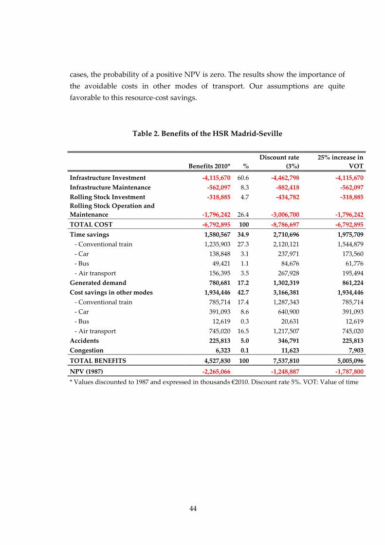
44

cases, the probability of a positive NPV is zero. The results show the importance of

the avoidable costs in other modes of transport. Our assumptions are quite

favorable to this resource-cost savings.

Table 2. Benefits of the HSR Madrid-Seville

Benefits 2010* %

Discount rate

(3%)

25% increase in

VOT

Infrastructure Investment -4,115,670 60.6 -4,462,798 -4,115,670

Infrastructure Maintenance -562,097 8.3 -882,418 -562,097

Rolling Stock Investment -318,885 4.7 -434,782 -318,885

Rolling Stock Operation and

Maintenance -1,796,242 26.4 -3,006,700 -1,796,242

TOTAL COST -6,792,895 100 -8,786,697 -6,792,895

Time savings 1,580,567 34.9 2,710,696 1,975,709

- Conventional train 1,235,903 27.3 2,120,121 1,544,879

- Car 138,848 3.1 237,971 173,560

- Bus 49,421 1.1 84,676 61,776

- Air transport 156,395 3.5 267,928 195,494

Generated demand 780,681 17.2 1,302,319 861,224

Cost savings in other modes 1,934,446 42.7 3,166,381 1,934,446

- Conventional train 785,714 17.4 1,287,343 785,714

- Car 391,093 8.6 640,900 391,093

- Bus 12,619 0.3 20,631 12,619

- Air transport 745,020 16.5 1,217,507 745,020

Accidents 225,813 5.0 346,791 225,813

Congestion 6,323 0.1 11,623 7,903

TOTAL BENEFITS 4,527,830 100 7,537,810 5,005,096

NPV (1987) -2,265,066 -1,248,887 -1,787,800

* Values discounted to 1987 and expressed in thousands €2010. Discount rate 5%. VOT: Value of time

45

Table 3. Benefits of the HSR Madrid-Seville by O-D pairs

Benefits 2010* %

Discount rate

(3%) 25% increase in VOT

Infrastructure investment -4,115,670 60.6 -4,462,798 -4,115,670

Infrastructure maintenance -562,097 8.3 -882,418 -562,097

Rolling Stock Investment -318,885 4.7 -434,782 -318,885

Rolling Stock Operation -1,796,242 26.4 -3,006,700 -1,796,242

TOTAL COSTS -6,792,895 100 -8,786,697 -6,792,895

Madrid-Sevilla 2,552,687 56.4 4,254,088 2,813,928

Time savings 888,221

1,521,653 1,110,276

- Conventional train 589,022

1,009,082 736,278

- Car 100,575

172,299 125,718

- Bus 42,229

72,344 52,786

- Air transport 156,395

267,928 195,494

Generated demand 432,874

719,775 472,060

Cost savings 1,231,592

2,012,660 1,231,592

- Conventional train 321,082

524,711 321,082

- Car 155,023

253,338 155,023

- Bus 10,466

17,104 10,466

- Air transport 745,020

1,217,507 745,020

Madrid-Cordoba 661,683 14.6 1,111,759 762,212

Time savings 284,135

486,174 355,169

- Conventional train 245,775

420,537 307,218

- Car 32,560

55,712 40,700

- Bus 5,801

9,926 7,251

Generated demand 209,210

350,793 238,705

Cost savings 168,338

274,791 168,338

- Conventional train 111,634

182,229 111,634

- Car 55,165

90,051 55,165

- Bus 1,539

2,512 1,539

Cordoba-Sevilla 95,252 2.1 160,716 106,017

Time savings 32,980

57,039 41,225

- Car 0

0 0

- Conventional train 31,589

54,633 39,486

- Bus 1,391

2,406 1,739

Generated traffic Rest 28,455

47,797 30,975

Cost savings 33,817

55,880 33,817

- Car 12,024

19,868 12,024

- Conventional train 21,178

34,996 21,178

- Bus 615

1,016 615

Commuting Services 878,947 19.4 1,471,358 972,399

Time savings 340,319

584,976 425,399

- Conventional train 340,319

584,976 425,399

- Car 0

0 0

Generated demand 97,567

162,702 105,940

Cost savings 441,061

723,680 441,061

- Conventional train 293,764

481,999 293,764

- Car 147,297

241,680 147,297

Others O-D 107,126 2.4 181,475 116,823

Time savings 34,912

60,853 43,640

- Conventional train 29,198

50,893 36,498

- Car 5,714

9,959 7,142

Generated demand 12,575

21,251 13,545

Cost savings 59,639

99,371 59,639

- Conventional train 38,055

63,408 38,055

- Car 21,583 35,963 21,583

Accidents 225,813 5.0 346,791 225,813

Congestion 6,323 0.1 11,623 7,903

TOTAL BENEFITS 4,527,830 100.0 7,537,810 5,005,096

NPV (1987) -2,265,066 -1,248,887 -1,787,800

* Values discounted to 1987 and expressed in thousands €2010. Discount rate 5%. VOT: Value of time

46

Figure 7. Probability distribution of the NPV Madrid-Seville

NPV1987 in €2010

0

0,2

0,4

0,6

0,8

1

1,2

1,4

1,6

1,8

-3

-2,8

-2,6

-2,4

-2,2 -2

-1,8

-1,6

Val

ues

x 1

0-9

Values in Billions

6. Ex-post evaluation of the Madrid-Barcelona HSR line

We are unaware of any comprehensive cost-benefit analysis of the Madrid-

Barcelona HSR line. In this section we undertake a full cost-benefit analysis of the

investment in the Madrid-Barcelona HSR line. It is not an ex ante CBA as the

construction started in 1999, and was completed in 2007, but it became partially in

service between Madrid and Zaragoza in 2003 (services between Madrid and

Barcelona in 2008). Nevertheless, although we are conducting this study in 2011,

the official information available for the CBA is not as good as one would expect

for a public investment. However, we have gathered some data from different

sources and, based on some reasonable assumptions for the reconstruction of the

unavailable information, have been able to calculate some sort of in media res NPV.

In what follows we describe the CBA of the Madrid-Barcelona HSR line and

discuss the probability distribution of the net present values obtained in the risk

47

analysis. The results seem to be robust within the ranges of the main parameters

and variables, given the available information.

The investment in 621 km of high speed infrastructure joining Madrid and

Barcelona allows a faster rail service in different O-D (Madrid-Barcelona, Madrid-

Zaragoza, Zaragoza-Lleida among others). The construction started in 1999 and

opened between Madrid and Zaragoza in 2003, and finally with Barcelona in 2008.

The total investment cost (land costs and stations excluded) was €9.5 billion of 2008

(Sánchez-Borrás, 2010). In contrast with the evaluation of the Madrid-Seville line,

where the actual construction costs per year were known, the investment costs of

the Madrid-Barcelona line were distributed during the construction period. The

investment costs of the route Madrid-Zaragoza were distributed within the period

1999-2003, considering the number of kilometers built per year. The same

procedure is followed for Zaragoza-Barcelona during the period 2003-2007.

Investment costs are inclusive of indirect and income taxes. The reason why

we have not accounted for the investment costs net of taxes is because planning

costs, land values and the construction costs of the stations and other facilities were

not included in the investment cost of the line. The project is assumed to have an

economic life of 50 years, and for simplicity we ignore any potential residual

value.9

The maintenance cost of the infrastructure per kilometer is 100,000 €/km in

2009. We assume half of these costs correspond to labor, and in the case of the

operation and maintenance of the rolling stock, we assume all costs are labor. The

shadow price of labor is based on Del Bo et al. (2009), where a conversion factor of

0.9 is estimated for Spain; and the other half of infrastructure maintenance is

computed net of indirect taxes (see Appendix 6.1 for more detailed information).

The maintenance and operation cost per train is 6.7 million in €1998 (de Rus and

Inglada, 1993).

For the estimation of total operating costs we need the number of trains and

the price of these trains. We assume the cost of a train follows a random uniform

distribution with range between €33,000 and €65,000 per seat in 2002 and each train

9 The main results do not change when the usual ad hoc percentages of the investment are

included at the end of the lifespan of the project.

48

has an average capacity of 330 seats and an economic life of 30 years (Campos et al.,

2009).

We assume demand is distributed uniformly during the day (no peak hours).

The load factor follows a random uniform distribution within the range 0.6-0.7. The

number of daily services required, given the load factor, the contingency factor, the

length of the route and the hours of operation are computed according to Campos

et al. (2009). Trains operate 16 hours per day and do not exceed the maximum

number of kilometers per year (500,000 km).

Other general assumptions affecting key parameters are the following: the

annual growth rate of income is taken from the National Institute of Statistics until

2009. From 2010 to 2015, the estimated growth rate is equal to 1% according to the

IMF. For the rest of the evaluation period, the annual growth rate follows a random

uniform variable between 1% and 4%, independent between years. The net present

value is calculated at the beginning of 1999 with benefits and costs expressed in

€1998 prices deflated with the CPI of the National Institute of Statistics. The social

discount rate of the base case is 5% and the shadow multiplier of public funds is 1.

The HSR travel time between Madrid and Barcelona is around 3 hours, and

many passengers benefit from these time savings, although as we will see, the

picture is quite different depending on which transport modes passengers were

initially traveling. Moreover, it is revealing to distinguish between the changes in

generalized costs and the differences in resource costs, ignoring transfers.

For the period 2003-2009, the demand is based on real data while for the rest

of the project life we have projected the number of passenger-trips of previous

years, assuming that the demand-income elasticity is equal to 1.

In 2009, the HSR transported 5.5 million passenger-trips in the whole line: 2.6

million between Madrid and Barcelona; 1.9 million between Madrid-Zaragoza or

Zaragoza-Barcelona and the rest between some other O-D.

The estimation of the diverted demand from the different modes per O-D and

year is based on the demand of that year in the route multiplied by the percentage

of the diverted demands that are presented in Appendix 6.1 under the heading

49

“modal split”. The distribution of the deviated demand is calculated using data

from the National Association of Highways (ACESA, 2009), ADIF and our own

estimation.

In the case of the O-D Madrid-Barcelona line, the origin of HSR passenger-

trips is as follows: 43% (plane); 27.3% (train); 16.1% (car); 3.2% (bus) and 10.4%

(generated). In the O-D Madrid-Zaragoza and Zaragoza-Barcelona: 2.7% (plane);

49.3% (train); 20% (car); 1.3% (bus) and 26.7% (generated). Let us concentrate in

two of the main corridors, Madrid-Barcelona and Madrid-Zaragoza to follow the

source of benefits.

Figure 8. Door-to-door trip time (Madrid-Barcelona)

0

1

2

3

4

5

6

7

8

9

10

HSR Plane Bus Car Conventional

Train

Ho

urs

Access and Egress Waiting In-vehicle

Figure 8 shows that the faster way to travel between Madrid and Barcelona

is by air. Door-to-door travel time is shorter, though the comparative advantage

rests on the substantially shorter in-vehicle time as the access-egress and waiting

time are higher when the airport infrastructure is involved. Nevertheless, even

accounting for the higher values of access-egress and waiting time, the door-to

door travel-time cost of is still slightly favorable to air transport (Figure 9).

50

Figure 9. Time-saving benefits per passenger-trip (Madrid-Barcelona)

0

20

40

60

80

100

120

140

160

180

200

Plane HSR Bus HSR Car HSR CT HSR

Plane Bus Car Conventional

Train

Eu

ros

20

10

Access and Egress Waiting In-vehicle

Figure 9 is illustrative in one sense. Average time benefits from deviated

demand are mainly concentrated in passengers already using railways. The

average time benefit is also high for passengers shifting from buses, but is not

relevant in absolute terms given the limited number of bus users. The time benefits

per passenger-trip shifting from air transport is negative and 43% of the deviated

demand comes from this mode of transport (we assume zero savings in the

evaluation).

However, individual modal choice is not based on resource costs but on the

generalized cost of travel; i.e., door-to-door trip time multiplied by the value of

time of passengers plus the money cost. Figure 10 is illustrative of the strong modal

competition in this O-D.

51

Figure 10. Generalized cost per passenger-trip (Madrid-Barcelona)

0

50

100

150

200

250

Plane HSR Bus HSR Car HSR CT HSR

Plane Bus Car Conventional

Train

Eu

ros

2010

Time component Price

The average generalized cost of HSR is similar for passengers initially

traveling by air. The comparison of generalized costs of car and HSR does not

consider that one option is to go by car between Barcelona and Madrid using the

toll road, which would make the generalized cost by car higher. In any case, the

participation of car passenger-trips in the deviated demand is quite low.

Air transport and HSR generalized costs are quite close, but we are using

averages and the money cost by air is, in the case of some airlines, substantially

lower than the average value behind Figure 10. The point is that the airlines still

keep half of the air/rail market and this means that there are 50% of the passengers

with lower generalized costs by air. From the information shown in Figure 10, the

key importance of the monetary component of the generalized cost and, in

particular, the pricing policy of the government with respect to the recovery of

infrastructure costs (see Section 8), seem evident. The importance of the efficiency

in airport management affecting delays and safety measures are also evident

according to the proximity of the generalized costs.

The shorter O-D Madrid-Zaragoza shows that air transport has the lower in-

vehicle time though the advantage of HSR is clear when door-to-door travel time is

the benchmark (Figure 11). Nevertheless, looking at Figure 12, total time cost is

52

quite close in the case of car trips. The reason is that although in-vehicle time is

shorter by HSR, a car passenger-trip shifting to HSR has to add access-egress and

waiting time, with higher value than in-vehicle time. The advantage of HSR with

respect to air is maintained when we add the money costs as portrayed in Figure

13, and though the advantage of HSR rail remains unchallenged the pricing policy

of the public sector with respect to the final modal split seems critical. For cars the

situation is quite different. Figure 13 shows a small advantage of cars over HSR

and a remarkable equality in all the transport modes but air.

Figure 11. Door-to-door trip time (Madrid-Zaragoza)

0

1

2

3

4

5

6

HSR Plane Bus Car Conventional

Train

Ho

urs

Access and Egress Waiting In-vehicle

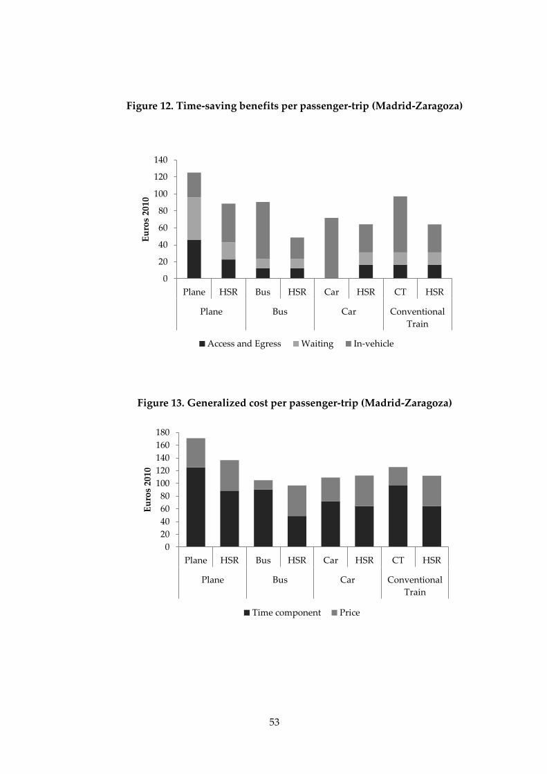
53

Figure 12. Time-saving benefits per passenger-trip (Madrid-Zaragoza)

0

20

40

60

80

100

120

140

Plane HSR Bus HSR Car HSR CT HSR

Plane Bus Car Conventional

Train

Eu

ros

20

10

Access and Egress Waiting In-vehicle

Figure 13. Generalized cost per passenger-trip (Madrid-Zaragoza)

0

20

40

60

80

100

120

140

160

180

Plane HSR Bus HSR Car HSR CT HSR

Plane Bus Car Conventional

Train

Eu

ros

2010

Time component Price

54

The observation of Figures 8 to 13 points out the source of the social benefits

from time savings. An inspection of Table 4 shows that total time savings represent

39% of the total benefits of HSR investment, basically from previous rail users. The

time benefits from air, car and bus are quite small. The condition required for social

profitability consisting of many passengers shifting to HSR and willing to pay a

high amount for the change, is not fulfilled in this corridor and this is a heavy

burden for the social profitability of the project given the magnitude of the

investment costs. More than 70% of the time-saving benefits come from for already

existing rail users.

Social benefits do not only come from time savings but also for the

additional willingness to pay from new passenger-trips and the avoidable costs in

the alternative modes of transport. Additional passenger-trips of new or existing

users in the corridors, account for 15% of total benefits, and the resource costs

avoided, thanks to the new rail line, account for 41% of the total benefits of the

project. The reduction of accidents accounts for 4.6% of the benefits. Congestion

savings are negligible.

The NPV of the Madrid-Barcelona HSR line refers to 1999, when the

construction started, though Tables 4 and 5 express the values in Euros of 2010.

This may seem trivial but many of the limited information about the construction

costs of different lines built in different moments of time is provided without

identifying the year when the line was built or whether the figures are in constant

or current terms.

The expected 1999 net present value is negative, equals to €-5.26 billion in

€2010, as shown in Tables 4 and 5, and this is 66.4% of the construction costs. The

risk analysis shows that the probability of having a positive NPV is zero. In fact,

the best result shown in the density function of NPVs is €-4.25 billion (see Figure

14). Although one should be cautious, given the limited information available, the

cost-benefit analysis of the line is conclusive in terms of the low value for money of

this investment.

The results obtained in the economic evaluation of the Madrid-Barcelona

HSR line reflect several undisputable facts: demand is extremely low. Only 2.6

million passenger-trips travel the whole length of the line. The other 3 million only

55

cover half of the length or less. The majority of passengers were initially traveling

by conventional rail, or by air, where the time benefits are quite low. The massive

fixed costs of the line (63.8% of total costs) and the fact that variable costs are

higher than the benefits from time savings and generated demand show that this

investment requires a higher volume of demand to be socially worthy.

The sensitivity analysis in Tables 4 and 5 shows the results are quite robust

to a lower social discount rate (3%) or an increase in the time savings benefits of

25% to account for willingness to pay for HSR higher comfort, service quality, or

whatever. In both cases the expected NPV is negative and the probability of a

positive NPV is zero. The results show the importance of the avoidable costs in

other modes of transport. Our assumptions are quite favorable to this resource cost

savings. If this were not the case, the economic implication would be much more

serious.

When the line was partially in operation, with trains running between

Madrid and Zaragoza, and the extension to Barcelona was still under construction,

de Rus and Román (2005) estimated the required first-year demand for a positive

social NPV. In that paper we surveyed passengers in the Madrid-Barcelona

corridor. From the estimated values of time and willingness to pay for comfort, the

time savings and the sources of deviated demand, we figured out some demand

thresholds required for a positive net present value. We showed that under

different assumptions regarding the demand growth rate, proportion of generated

demand, time savings and users willingness to pay for those savings, a demand

above 10 million passenger-trips would be required in the first year of operation,

twice the actual demand.

We have calculated the volume of demand required for a positive NPV

within the cost-benefit framework of this report. The minimum demand required

for a positive NPV in the first year of operation of the whole length of the line is

12.3 million passenger-trips (keeping the same distribution per O-D). This figure

contrasts with the actual demand of 5.5 million passenger-trips in 2008.

56

Table 4. Benefits of the HSR Madrid-Barcelona

Benefits 2010* % Discount rate (3%) 25% increase in VOT

Infrastructure Investment -7,923,236 63.8 -8,548,659 -7,923,236

Infrastructure Maintenance -844,685 6.8 -1,335,589 -844,685

Rolling Stock Investment -397,045 3.2 -532,523 -397,045

Rolling Stock Operation and

Maintenance -3,257,395 26.2 -5,632,903 -3,257,395

TOTAL COST -12,422,362 100 -16,049,674 -12,422,362

Time savings 2,795,246 39.0 4,937,790 3,494,057

- Conventional train 2,049,265 28.6 3,616,583 2,561,582

- Car 550,192 7.7 974,680 687,740

- Bus 158,727 2.2 282,271 198,409

- Air transport 37,062 0.5 64,256 46,327

Generated demand 1,076,442 15.0 1,843,246 1,192,774

Cost savings in other modes 2,936,053 41.0 4,974,387 2,936,053

- Conventional train 885,858 12.4 1,489,207 885,858

- Car 723,302 10.1 1,220,151 723,302

- Bus 62,977 0.9 107,295 62,977

- Air transport 1,263,916 17.7 2,157,734 1,263,916

Accidents 329,969 4.6 590,943 329,969

Congestion 20,434 0.3 33,082 25,543

TOTAL BENEFITS 7,158,145 100 12,379,448 7,978,397

NPV (1999) -5,264,217 -3,670,226 -4,443,965

* Values discounted to 1999 and expressed in thousands €2010. Discount rate 5%. VOT: Value of time

57

Table 5. Benefits of the HSR Madrid-Barcelona by O-D pairs

Benefits 2010* % Discount rate (3%) 25% increase in VOT

Infrastructure investment -7,923,236 63.8 -8,548,659 -7,923,236

Infrastructure maintenance -844,685 6.8 -1,335,589 -844,685

Rolling Stock Investment -397,045 3.2 -532,523 -397,045

Rolling Stock Operation -3,257,395 26.2 -5,632,903 -3,257,395

TOTAL COSTS -12,422,362 100 -16,049,674 -12,422,362

Madrid-Barcelona 3,856,107 53.9 6,710,367 4,254,165

Time savings 1,460,888

2,607,969 1,826,110

- Conventional train 1,020,209

1,821,272 1,275,262

- Car 303,098

541,090 378,873

- Bus 137,580

245,607 171,975

- Air transport 0

0 0

Generated demand 422,689

732,249 455,524

Cost savings 1,972,531

3,370,149 1,972,531

- Conventional train 361,388

617,446 361,388

- Car 320,010

546,749 320,010

- Bus 57,595

98,403 57,595

- Air transport 1,233,539

2,107,551 1,233,539

Madrid-Zaragoza/Zaragoza-Barcelona 1,802,450 25.2 3,059,621 2,053,128

Time savings 735,290

1,274,816 919,113

- Conventional train 619,952

1,074,847 774,940

- Car 57,130

99,050 71,413

- Bus 21,147

36,664 26,434

- Air transport 37,062

64,256 46,327

Generated demand 524,172

887,794 591,028

Cost savings 542,987

897,011 542,987

- Conventional train 344,912

569,791 344,912

- Car 162,316

268,144 162,316

- Bus 5,382

8,892 5,382

- Air transport 30,377

50,183 30,377

Others O-D 1,149,184 16.1 1,985,434 1,315,592

Time savings (deviated traffic): 599,068

1,055,005 748,835

- Car 189,964

334,541 237,455

- Conventional train 409,104

720,464 511,380

Ggenerated traffic 129,581

223,203 146,222

Cost savings 420,535

707,227 420,535

- Car 240,976

405,257 240,976

- Conventional train 179,559 301,970 179,559

Accidents 329,969 4.6 590,943 329,969

Congestion 20,434 0.3 33,082 25,543

TOTAL BENEFITS 7,158,145 100 12,379,448 7,978,397

NPV (1999) -5,264,217 -3,670,226 -4,443,965

* Values discounted to 1999 and expressed in thousands €2010. Discount rate: 5%. VOT: Value of time

58

Figure 14. Probability distribution of the NPV Madrid-Barcelona

NPV1999 in €2010

0

0,1

0,2

0,3

0,4

0,5

0,6

0,7

0,8

0,9

1

-6,5 -6

-5,5 -5

-4,5 -4

Val

ues

x 1

0-9

Values in Billions

7. Ex-ante evaluation of the Stockholm-Gothenburg

HSR line

The revision of the existing evaluations of the projected lines Stockholm-

Gothenburg-Malmo shows different results regarding the expected economic

profitability of the project. Nilsson and Pyddoke (2009), based on a CBA report

commissioned by the Swedish National Rail Administration, report a negative

NPV for the Stockholm-Gothenburg line and discuss whether some

underestimation of the environmental benefits could compensate the poor socio-

economic result obtained in the economic evaluation (benefits account for 80%

of social costs). They examine whether the benefits derived from the release of

59

capacity for freight and the contribution to the reduction of CO2 are high

enough to reach a positive NPV.

In Jansson and Nelldal (2010) the starting point is that the Stockholm-

Gothenburg line is socially worthy. They refer to two CBA reports by the

consultant WSP and by the Royal Institute of Technology (KTH), both with a

positive NPV. The benefits from freight, in WSP, are 14.7% of total benefits and

13.8% in KTH. The external effects (including accidents) are 22.4% and 13.2% of

total benefits in WSP and KTH respectively. Therefore, the issue of the potential

environmental benefits of the HSR investment in Sweden is noteworthy and so

we deal with it separately at the end of this section.

In this paper, we do not try to estimate a new figure for the economic

profitability of the HSR project in Sweden. The main reason is the lack of data.

Moreover, we are unable to comment on the results obtained in previous

evaluations as the demand data supporting the calculus of the social surplus are

not disclosed in these studies. What we do here, based on Lindgren (2009),

Swepro (2009), WSP (2010), de Rus (2010) and de Rus et al. (2009), is to start with

some basic supply data on investment costs, some ranges on acquisition of

rolling stock and operation and maintenance in Europe; and, on the demand

side, we rest on the estimation of values of time and modal split with and

without the project reported in Börjesson (2011). This last reference is crucial for

the exercise below.

Instead of the calculus of the NPV, we invert the process and estimate the

minimum demand volume compatible with a positive NPV, given a set of

explicit assumptions on costs and demand. Then, we change the values of the

main parameters to cover the most probable cases to obtain the corresponding

demand thresholds within a wide range of possibilities. We focus on the

Stockholm-Gothenburg, and only accounting for the direct benefits. We do not

include the line to Malmo or the alleged benefits of freight transport (though we

include this last benefit in the sensitivity analysis), congestion and accidents

(none significant), nor environmental externalities (separately discussed).

Evidence from other studies and the results of the two Spanish lines

evaluated in previous sections of this paper show that benefits deriving from

60

the reduction of congestion and accidents are less than 5% of total benefits and,

in the case of Sweden, the prediction of changes in modal split with the project

show that car passenger-trips shifting to HSR are less than 3% of the total

passenger-trips in the first year of operation.

The benefits of avoided road accidents should be lower than in the case of

Spain because the lower percentage of victims in road accidents per inhabitant

in Sweden. The number of killed people per million of inhabitants in road

accidents in Sweden is considerably lower than most European countries. Thus,

there were 39 victims per million of inhabitants for Sweden while Spain had a

rate equal to 59 (Eurostat, 2009). In the case of the Stockholm region, the

situation is even better with a rate of 17 victims per million of inhabitants. The

value of a statistical life is, according to Heatco (2006), €1,122,000 in Spain and

€1,870,000 in Sweden.

Once we obtain the minimum demand thresholds needed for a positive

NPV under these assumptions, we conduct a sensitivity analysis with the

introduction of freight benefits reported in Swepro (2009) and WSP (2010). A

discussion of the potential environmental benefits is carried out at the end of the

section.

The main assumptions and data of the exercise are the following. The

construction period of the Stockholm-Gothenburg starts in 2010 and lasts until

2024 (WSP, 2010). The first year of operation is 2025 and the project life is 50 and

100 years alternatively. It may well be that 100 years is a too long a period, given

technological change in rail and the competing modes of transport, but this is

the length assumed in some of the existing reports in Sweden, and so we

simulate the situation with this lifespan and also with 50 years. No residual

value is considered.

The flow of benefits and costs are discounted with a 5% discount rate and

alternatively with a 4% rate. The annual growth rate of income is based on IMF

statistics until 2016. For the rest of the evaluation period, the annual growth rate

is assumed to be 2.5%. Prices are deflated with the Swedish CPI. Benefits and

costs are assumed to be realized at the end of the year. Benefits and costs are

61

expressed in €2010. The shadow multiplier of public funds is 1. Exchange rate 1

€ = 10 SEK.

Total investment costs are €10.5 billion (2008). Investment costs have been

distributed during the construction period. VAT was not deducted, nor is cost

overrun considered. The maintenance cost of the infrastructure is 100,000 €/km

in 2009, 50% of infrastructure maintenance costs correspond to labor and VAT is

25% during the whole period. The tax is deducted from 50% of the non-labor

maintenance costs. According to different sources in the rail industry, and

considering the average wage in Sweden, the operation and maintenance costs

of the rolling stock per seat-kilometer is assumed to be €0.06 in €2010. We

assume that labor is the main component of this unit cost and that unit labor

costs are constant or increase proportionally with real income.10

The cost of the HSR rolling stock in Europe varies widely depending on

several technical characteristics and capacity options as explained in Section 2.

We assume that the cost of a train set is the average between the minimum and

the maximum values in the database (€33,000 and €65,000 per seat in 2002). The

average capacity per train is 370 seats (de Rus et al., 2009). VAT was not

deducted in the acquisition of the rolling stock. The main reason is that the

rolling stock is mostly an imported technology. The average life of a train is 30

years.

The number of daily services required, given the demand, the travel time,

the load factor, the length of the route and the hours of operation are computed

according to de Rus et al. (2009). Based on a previous formula, applying a

contingency factor (1.5) is required, in order to deal with operating and

maintenance constraints. Moreover, trains cannot exceed a maximum number of

kilometers per year (500,000 km.). Therefore, the final number of trains is

computed as the maximum between these two previous rules. Operating train

time includes the time between train-trips. It is assumed to be 15 minutes. We

assume the load factor equal to 0.65 and 17 hours of operation.

10

In the first draft of this report, we used data from the UIC for the operating and maintenance

costs. These figures seem to be incorrect and we have changed to a more reliable source. We

truly appreciate the help of Pablo Vázquez (INECO) with the revision of the cost data.

62

Traffic deviation from conventional modes of transport to HSR reduces the

activity in these modes and it is assumed that the average avoidable cost in

other modes of transport equals their prices net of indirect taxes. These prices

are taken from different sources and though they are approximations to the

actual avoidable costs, we expect that any possible bias is in favor of the project.

The average price for the airlines in the Stockholm-Gothenburg route is

collected from different travel websites. This value is multiplied by 0.8 to

account for the presence of the low-cost airlines in the corridor and shadow

pricing. The average prices of a bus-trip are taken from the website of SWEBUS.

A conversion factor of 0.9 is applied to account for shadow pricing. Prices of the

conventional train are taken from the website of SJ. A conversion factor of 0.8 is

applied to account for shadow pricing. The cost of a car-trip is approximated

from different sources and follows the basic argument of Sections 5 and 6. An

occupancy factor of 1.3 is assumed to convert passenger-trips into car-trips.

Annual demand is assumed to grow, according to the national forecast

model, with a demand-income elasticity of 0.512 (Börjesson, 2011). Alternatively

we introduce the value of 1. The generated and diverted traffic from the

different modes and year are computed as the demand of that year in the route

multiplied by the percentage of the diverted traffic of the following modal split

proportions (Börjesson, 2011): diverted traffic from air: 4.44%; bus: 0.18%; car:

2.47%; conventional train: 71.61%. The coefficient of the generated traffic:

21.30%.

Time-saving benefits and the willingness to pay of generated demand are

obtained with the ‘rule of a half’. A basic parameter in this calculus is the value

of time. Values of in-vehicle time for plane, bus, car and conventional train and

for business and private purposes are taken from Börjesson (2011). Waiting-time

values are assumed to be 1.5 times the corresponding values of in-vehicle time.

Values of access/egress time are computed as 2 times the values of in-vehicle

time (Wardman, 2004). The elasticity of the value of time with respect to income

is 0.7 (Mackie et al., 2001; Heatco, 2006). Waiting times of HSR, bus and

conventional train are assumed to be the same. Access and egress time of the

HSR, bus and conventional train are assumed to be the same.

63

Table 6 summarizes the results of the simulations. It displays the

minimum level of passenger-trips required for a positive NPV, given the

assumptions and data described above. A quick look shows how these figures

compare with the forecasted demand in this corridor in its first year of

operation. Börjesson (2011) predicts 1.6 million for the Stockholm-Gothenburg

corridor in 2010, a figure that it is far from the demand thresholds required for

the investment to be socially worthy in the more realistic cases.

Table 6. First-year demand thresholds for a positive NPV

(passenger-trips, millions)

Note: In brackets, first year passenger-trips with a 4% and 5% discount rate.

(*) Demand-income elasticity

In the cases where the demand-income elasticity is assumed to be 0.512

(the value estimated for Sweden), labor costs grow proportionally with income

and half of the passenger-trips travel the whole length of the line, the demand

thresholds for a NPV equal to zero go from 17 to 25 million of passenger-trips in

the first year operation.

There are other more favorable scenarios where the required demand

levels for the first year of operation could be lower but the underlying

assumptions are then somewhat unrealistic.

Project life (years)

50 100

% passengers travel the whole

length

% passengers travel the whole

length

100 50-50 100 50-50

Lab

or

cost

s

gro

w

wit

h i

nco

me

yes

Ela

stic

ity

* 0.512 (10.3 –12.8) (19.8 – 24.6) (8.2 – 11) (16.6 – 21.8)

1 (6.3 – 8.1) (10.5 – 13.7) (3.6 – 5.5) (5.7 – 8.9)

no

0.512 (7 – 8.9) (10.5 – 13.5) (4.9 – 7.1) (7.4 – 10.6)

1 (5 – 6.6) (7.6 – 10) (2.9 – 4.5) (4.2 – 6.7)

64

The released capacity for freight transport has been argued to be one of the

benefits of the construction of HSR infrastructure in Sweden. According to

Jansson and Nelldal (2010), “the High-Speed Line also releases capacity on the

Southern and Western Main Trunk Lines for freight and fast regional trains. At

the moment there are conflicts here, especially between high-speed trains on the

one hand and regional and heavy goods trains on the other. With high-speed

trains using the High-Speed lines, the Southern Main Line can satisfy the

industry’s growing need for efficient export and import of raw materials. It is

important for the industry to be able to offer direct, high-capacity, highly

punctual trains to the continent.”

To conclude this exercise, Table 7 recalculates the minimum demand

volumes compatible with a positive NPV including the alleged benefits derived

from the release of capacity for freight transport. The inclusion of freight

benefits in the calculus of the demand thresholds has been done according to

WSP (2009) which considers that these benefits have a net approximate present

value of €640 million (2010). Given that there exist some uncertainty around

these figures because it also requires new investments in terminals and lines, we

consider a minimum value of €580 million and a maximum of €1 billion (2010).

The way in which we deal with the uncertainty of freight benefits in the

calculus of the minimum volumes of demand compatible with a positive NPV,

is to add the expected present value of freight benefits of €790 million to the

benefits of the project. The figures do not show any dramatic change with

respect to the demand threshold of Table 6. Moreover, we have recalculated the

demand thresholds of tables 5 and 6 with an operating and maintenance cost

per seat-km of €0.05 without significant changes in the results.

65

Table 7. First-year demand thresholds for a positive NPV

including freight benefits

(passenger-trips, millions)

Project life (years)

50 100

% passengers travel the whole

length

% passengers travel the whole

length

100 50-50 100 50-50

Lab

or

cost

s

gro

w

wit

h i

nco

me

yes

Ela

stic

ity

* 0.512 (9.3 – 11.4) (17.9 – 21.8) (7.4 – 9.8) (15 – 19.4)

1 (5.7 – 7.2) (9.5 – 12.2) (3.2 – 4.9) (5.1 – 7.9)

no

0.512 (6.2 – 7.8) (9.4 – 11.9) (4.4 – 6.2) (6.6 – 9.4)

1 (4.5 – 5.8) (6.8 – 8.8) (2.6 – 3.9) (3.8 – 5.9)

Note: In brackets, first year passenger-trips with a 4% and 5% discount rate.

(*) Demand-income elasticity.

Environmental benefits

The results obtained in this paper show that, in a wide range of circumstances,

the social benefits of HSR investment do not cover total social costs for any

demand volume, and in the best scenarios the required volume of demand for a

positive NPV seems to be too high compared with the potential traffic volumes

in the corridor. Nevertheless, as we have already mentioned, these conclusions

do not account for the potential environmental benefits of the project. Would the

inclusion of these benefits change the likely poor social profitability of this

project?

The stronger defense of investing in HSR, as a policy instrument for the

mitigation of global warming, can be found in Åkerman (2011). The analysis

deals with the Stockholm-Gothenburg-Malmo line using a life-cycle perspective.

The author estimates that the construction and maintenance of the line during

60 years produce 4 million tons of CO2 (66,000 tons per year) and 20% of these

emissions are due to permanent deforestation. The author estimates a life-cycle

66

reduction of 550,000 tons per year in CO2-equivalents thanks to changes in

modal split. These environmental benefits come from freight-traffic diversion

from road to HSR (60%) and passenger-traffic diversion from road and air to

HSR (40%). Hence it is crucial to see the assumptions behind the substitution

effects in order to consider the feasibility of compensating the 66,000 tons of

CO2 of construction and maintenance of the HSR line (in contrast, Kageson,

2009 shows a net reduction 90,000 tons for a 500km HSR line, ignoring the

emissions during construction).

One key assumption in Åkerman (2011) is that half of the diversion of

traffic from trucks to train rests on shifts from international traffic. The release of

capacity in the old track, thanks to the construction of a new HSR line for

passengers, is a necessary condition, according to the author, but not a sufficient

condition for the increased rail freight. He proposes further measures to

materialize the change with the project: increased axle load, development of

intermodal freight, improved capacity across the Öresund Strait and in

Denmark, and a fully deregulated rail freight market in the EU.

The other half of the environmental benefits in Åkerman (2011) comes

from the deviation of passenger traffic from road and air to HSR. The argument

justifying the substitution effect is somewhat weak. It is basically based on the

assumption that changes in modal split observed in some European routes in

operation, with special mention to the Spanish lines and the Paris-Lyon, can be

transferred to the Swedish lines. The author assumes an air/rail market share of

80% for the O/D Stockholm-Gothenburg and 65% for the O/D Stockholm-

Malmö.

This new modal split implicitly assumes that HSR prices are going to be

heavily subsidized in Sweden. HSR pricing is crucial for HSR demand as the

generalized prices are quite close given the actual travel times. The forecasted

demand for the Swedish lines is considerably lower than the actual demand in

the Paris-Lyon line, and the fixed cost per km is higher in Sweden. In the case of

Madrid-Seville and Madrid-Barcelona the demand volumes are, to some extent,

closer to the Stockholm-Gothenburg and the Stockholm-Malmö but the prices

are heavily subsidized and even so, the HSR in the Madrid-Barcelona line has

67

not yet gone beyond 50% of the air/rail market share. Unless pricing is explicitly

addressed, the projected market shares are somewhat speculative.

In the case of traffic deviation from cars to train the above argument also

applies. Besides, one should not expect dramatic changes as long as the option

of traveling by car within these distances has additional advantages (e.g. the

marginal cost of an additional passenger is zero). Moreover, the previous

existence of the air transport alternative plus a reasonable good conventional

train service between the main O/D recommend some prudence when

forecasting the deviation of passenger-trips from cars to HSR.

The comparison between the negative externalities during the construction

of the line and the positive externalities from the diversion of traffic from road

and air to HSR is further analyzed in Kageson and Westin (2010). The results do

not support the belief that investing in HSR is good for the environment. Using

a Monte Carlo simulation Kageson and Westin estimate, using more than 10

million annual one-way trips, the traffic volume required to balance the CO2

emission from the construction of a 500 km line. The authors conclude that from

a climate point of view it may be better to upgrade existing lines and to try to

make people substitute air travel by modern telecommunications rather than

investing huge amounts of resources in making us travel faster and more.

Nilsson and Pyddoke (2009) analyze whether the investment in the HSR

Stockholm-Gothenburg line may be justified as a cost-effective way of reducing

carbon dioxide emissions. Based on a study commissioned by the Swedish

National Rail Administration where social benefits only cover 80% of total costs,

they try to answer the question of whether the environmental benefits are

higher than those included in the Rail Administration report and also whether

there is underestimation of the benefits or overestimation of costs. The authors

do not have any evidence of any systematic bias and conclude that the

investment in the Stockholm-Gothenburg line is not an efficient alternative for

mitigating global warming for the following reasons.

The operation of the HSR line between Stockholm and Gothenburg would

reduce 150,000 tons of CO2 emissions per year from aircraft, trucks and

passenger road traffic which amounts to 0.7% of annual transport sector

68

emissions. The authors do not include the emissions during the construction

period. Kageson (2009) estimates that the embedded emissions generated from

the construction, maintenance and deconstruction of the railway track amount

to a total of 110,000 tons per year.

The value used for reduced emissions of CO2 in the economic evaluation

of the line is SEK 1.50 per kilo. Nilsson and Pyddoke (2009) consider that a more

reasonable value may be about SEK 0.40 per kg. “Using the assumptions

otherwise made by the Swedish National Rail Administration, a simple reverse

calculation shows that CO2 emissions would have to be valued at more than

SEK 8 per kilo for Götalandsbanan to be cost-effective for society. In terms of

taxation of petrol this corresponds to almost SEK 19 /litre or a petrol price of

more than SEK 30 per litre. In light of this it is difficult to see railway

investments as a cost- effective climate policy instrument.”

Nilsson and Pyddoke (2009) conclude that the poor results associated with

this project is mainly due to the fact that investment is a weak instrument for

achieving significant changes in emission volumes defending the internalization

of externalities: “An effective environmental policy requires general policy

instruments (for example fuel taxes) that target all passengers, not only the few

who travel on a specific route. Railway investments are generally therefore an

inefficient policy instrument.” This leads to our next section where the key issue

of pricing and changes in modal split is covered.

Before concluding this brief account on the existing studies of the potential

environmental impact of the HSR project in Sweden it is worth it to stress the

intrinsic difficulties with the construction of a plausible contrafactual. The base case

for a lifespan of 50 or 100 years from 2020 onwards requires a high proportion of

speculation about how environmental externalities develop. The expected

environmental benefits of the HSR investment are dependent on what is assumed

to happen with the alternative mode of transport during the life time of the project

and this implies plenty of guessing.

The construction of the contrafactual has to include predictions on the

construction of highways and airport infrastructure avoided and the development

of new technologies which may reduce the environmental externalities of road and

69

air transport. Also, it needs to account for a more efficient way to handle

congestion and safety, the application of more efficient pricing policies

internalizing the external effects and therefore reducing the effect of HSR

investment as a second best environmental policy.

8. Intermodal effects, pricing and CBA

The generalized cost of travel includes three basic components: time, quality

and money, understanding “quality” in a broad sense to include from comfort to

safety. The time component is far from being homogeneous. It includes access-

egress, waiting and in-vehicle time. In medium- distance corridors like the ones

evaluated in this paper, we have seen how close the time component may be

between HSR and the alternatives, and this concedes a key role to the pricing

policy of the public sector regarding the access to HSR infrastructure.

The 500-600 km intercity corridor with road, air and rail transport in open

competition have a modal-split equilibrium that is very sensitive to small changes

in the generalized costs of each mode of transport. The differences between air

transport, road and rail are evident, but they have several things in common. On

the supply side, they all need infrastructure to provide services combining vehicles,

labor and energy. In addition, infrastructure and operation may be vertically

integrated or unbundled. On the demand side, they all involve a transport service

carrying passengers who have to pay different generalized costs in terms of money,

time, and quality.

Air and road transport are vertically unbundled and different operators use a

common infrastructure, sometimes with free access and sometimes with payment

of an access fee (toll, price, etc.). Usually the operators are private and the

infrastructure is public or privately operated under a concession contract. Road

and air transport services are vertically separated from the infrastructure operator,

and railways are unbundled in some cases and vertically integrated de facto in the

case of high speed trains operated by a single firm with the exclusive use of

dedicated infrastructure.

70

Buses and cars share the same roads, competing airlines share airports, and

HSR is technically operated as a single business, even if, from an organizational

standpoint, the maintenance and operation of the infrastructure are separated from

service operations. HSR has other advantages over airlines beyond vertical

integration, reflecting some structural differences. Airports and airlines serve a

large number of markets using the same airport capacity, and it is not clear that

airport congestion management would be better with vertical integration. The HSR

advantage in this case is that capacity is used to serve a very small number of

markets (O-D pairs), and this makes it possible to reach very high levels of

reliability.

These differences on the supply side have significant impacts on the demand

side. The vertical integration of infrastructure and operation in the case of HSR is a

significant advantage with respect to air transport in terms of the generalized costs

of travel. HSR is more reliable than air transport, and though it increases in-vehicle

time with respect to air transport, it reduces access and egress (on average) and

waiting time. Airport and airline managers do not necessarily have the same

objectives and, as a matter of fact, the generalized cost advantage of HSR with

respect to air lies outside the travel-time segment of the trip. In the case of roads,

the differences are even clearer. Road infrastructure and operations are vertically

separated. In contrast to the single operator of HSR, there are many users driving

their own cars with free access in many cases to a limited-capacity infrastructure.

Road transport has the advantage of reducing access and waiting time to almost

nothing and the cost disadvantage appears in the travel-time segment.

Investment in HSR changes the equilibrium in the interurban corridor

through its impact on the generalized cost of rail travel. Compared with

conventional rail, HSR services barely affect access, egress and waiting time. The

main impact is on travel time with a magnitude depending on the prevailing

operating conditions of the conventional rail. Passengers shifting from road

transport benefit from travel-time reductions but lose in terms of access, egress and

waiting time. Those shifting from air transport may benefit from lower access-

egress and waiting time, but lose in terms of in-vehicle time. When the whole door-

to-door time is considered and weighted with the values of the time of each

component, we have found that, given the actual differences in the time-cost

component, the modal choice may be highly dependent on the money component.

71

Figures 15 to 18 show the generalized cost differential as well as the price

differential between HSR and its alternatives. One would expect the generalized

cost to be always lower for HSR as none would shift mode otherwise. The negative

dark bar confirms that this is the case for all the transport modes with some

exceptions: car in the case of the O-D Madrid-Zaragoza and Cordoba-Seville and

the conventional train in the case of Cordoba-Seville. The higher generalized cost

for HSR with respect to cars in Cordoba-Seville and Madrid-Zaragoza is

incompatible with the fact that the HSR has deviated demand from cars in these O-

D. There are two explanations for this inconsistency. First, the values in Figures 15

to 18 are averages and so are compatible with generalized costs below average for

some users. Second, the absolute positive values of the differences in generalized

costs are low enough to be compensated by any other unobserved elements of the

actual generalized cost of car users.

In the case of the O-D Cordoba-Seville the time saving is low and the increase

in price offsets the time advantage. Beyond data incompleteness, it is possible for

rail users to shift to HSR and to lose surplus in the process as long as the new HSR

services substitute the conventional trains.

Figure 15. Generalized cost and price differential of HSR with respect to other

transport modes (e.g., HSR-car)

Madrid-Barcelona

-80

-60

-40

-20

0

20

40

Plane Bus Car Conventional

Train

Eu

ros

2010

Generalized Cost Price

72

73

Figure 16.Generalized cost and price differential of HSR with respect to other

transport modes (e.g., HSR-car)

Madrid-Zaragoza

-40

-30

-20

-10

0

10

20

30

40

Plane Bus Car Conventional

Train

Eu

ros

2010

Generalized Cost Price

Figure17.Generalized cost and price differential of HSR with respect to other

transport modes (e.g., HSR-car)

Madrid-Seville

-80

-60

-40

-20

0

20

40

60

Plane Bus Car Coventional

Train

Eu

ros

2010

Generalized Cost Price

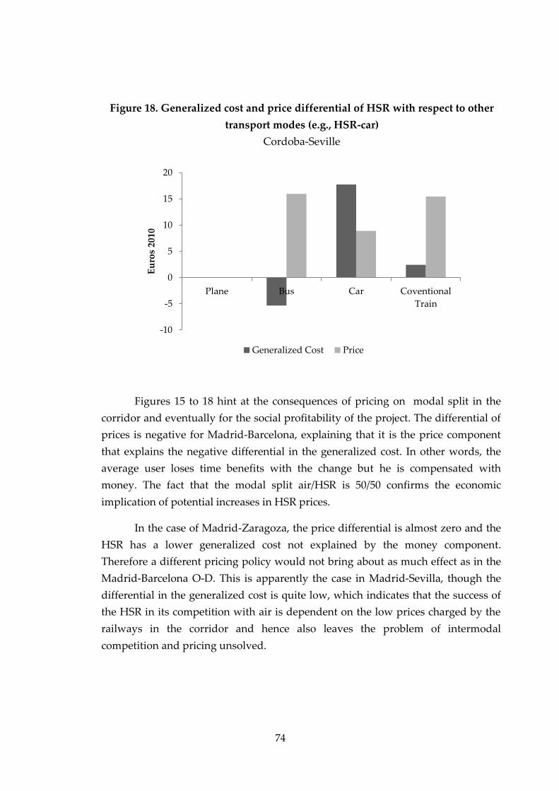
74

Figure 18. Generalized cost and price differential of HSR with respect to other

transport modes (e.g., HSR-car)

Cordoba-Seville

-10

-5

0

5

10

15

20

Plane Bus Car Coventional

Train

Eu

ros

2010

Generalized Cost Price

Figures 15 to 18 hint at the consequences of pricing on modal split in the

corridor and eventually for the social profitability of the project. The differential of

prices is negative for Madrid-Barcelona, explaining that it is the price component

that explains the negative differential in the generalized cost. In other words, the

average user loses time benefits with the change but he is compensated with

money. The fact that the modal split air/HSR is 50/50 confirms the economic

implication of potential increases in HSR prices.

In the case of Madrid-Zaragoza, the price differential is almost zero and the

HSR has a lower generalized cost not explained by the money component.

Therefore a different pricing policy would not bring about as much effect as in the

Madrid-Barcelona O-D. This is apparently the case in Madrid-Sevilla, though the

differential in the generalized cost is quite low, which indicates that the success of

the HSR in its competition with air is dependent on the low prices charged by the

railways in the corridor and hence also leaves the problem of intermodal

competition and pricing unsolved.

75

Pricing, modal split and investment

It seems clear (equity issues aside) that for the user´s choice to be socially optimal,

prices should reflect the opportunity costs of his choice. Efficiency requires a sound

pricing policy that not only allows the transport user to choose the best option

within a transport mode but also when choosing between air, rail or road transport.

Let us assume that supplier-operating costs, variable maintenance and

operating infrastructure, and external costs are already included in the generalized

cost. How much should a rail operator be charged for the use of the infrastructure

in a particular time or demand conditions? In principle, the answer is the `marginal

social cost´ of running the train in that particular situation. Given the presence of

economies of scale, significant indivisibilities and fixed and joint costs, pricing

according to marginal social costs is far from being an easy task.

Charging according to short-run marginal cost is incompatible with cost

recovery when the infrastructure rail network is built and there is excess of

capacity, as is the case of the HSR lines in this paper. Some critics argue that the

natural alternative is long-run marginal costs. Short-run marginal cost is equal to

the change in total costs when new demand is added, given a constant network

capacity. Long-run marginal cost accounts for the change in total cost allowing for

an optimal adjustment of capacity.

Long-run and short-run marginal costs are equal assuming perfect demand

forecast and perfect divisibility of capital, but both assumptions are unrealistic in

transport and consequences of choosing a pricing principle are quite important in

practical terms. For the case of HSR investment, short-run marginal cost pricing

means prices below average costs and the need for public funds to cover

infrastructure costs (see Rothengatter, 2003; Nash, 2003).

With a fixed capacity, any additional demand willing to pay in excess to the

additional cost imposed to the system should be attended. In the extreme case,

when capacity is well above demand (forecasting error, indivisibilities or both)

short-run marginal cost can be very low compared to average cost. Many argue that

passengers should only pay the short-run marginal costs but there are other reasons

to charge about the strictly avoidable cost. The first reason is the problem of

76

financing the infrastructure costs. Additional taxation needed to cover the gap has

an additional cost in terms of the distortion imposed on the rest of the economy.

The second problem is related to incentives, as subsidization usually reduces effort

to minimize costs. Another drawback comes from the way in which capacity costs

are covered, as users only pay variable costs and non-users pay capacity costs. In

addition to the equity side (it is difficult to think of HSR passengers as equity

targets) we face a dynamic efficiency question: are the users willing to pay for

capacity? In the corridors where this is not the case, the government would be

providing more capacity than optimal.

Even assuming that users are willing to pay for capacity (given prices equal

to short-run marginal costs), it may be argued that demand is receiving a

misleading signal in terms of the cost of expanding capacity in the long term. It

may well be that a price structure which includes some charges for long-term

replacement costs would be associated with a social surplus insufficient to justify

the investment.

The consequences of charging according to the short-run marginal cost on

the expansion of HSR lines are significant. Low prices favor the reallocation of

demand from the competing modes and encourage demand generation, with a

feedback on the future expansion of the network. Pricing according to short-run

marginal cost leaves a key question unanswered: are the rail users willing to pay

for the new HSR capacity? Unless this question is answered before investment

decisions are taken, marginal-cost pricing is not a guarantee for an efficient

allocation of resources.

The social marginal cost of a passenger-trip in particular mode of transport,

in a particular place and time, has three different parts: the user marginal cost (user

cost and the share of the producer cost –infrastructure and vehicles- included in the

price), to cost to the other users and the rest of society (congestion, external cost of

accidents and environmental externalities) and to the taxpayers (the share of the

producer cost that has been subsidized).

Revenue is far from covering total costs. It might be argued that economies

of scale and strong indivisibilities justify the deficits, but the question is that users

should be willing to pay for the HSR infrastructure before new lines are built. HSR

77

prices act as signals that transport users take as key information on where, how and

when to travel, or even whether to travel or not. When infrastructure costs are not

included in transport prices, according to the rationale of short-term marginal

social cost, the problem is that the price signal is telling consumers that it is efficient

to shift from road or air transport to rail transport, and this, of course, could be true

in the short-term when optimal prices are not affected by the fixed costs of the

existing HSR network, but the world is dynamic.

The problem is that prices that do not include fixed infrastructure costs

(around 60% of total costs) which act as long-term signals for the consumers in their

travel decisions, and consequently in the future allocation of resources between

transport modes or between transport, education or health. An extensive HSR

network can be developed based on suboptimal prices decided by the government

which keep no relation to the opportunity costs of its existence, but once the

network is built bygones are bygones, and the speculation on the counterfactual

with a different allocation of resources and their effect on welfare is not very

practical.

The defense of cost-benefit analysis in this context is quite relevant. Even

accepting that short-term marginal cost is the right pricing policy, investing in a

new HSR line requires that the willingness to pay for capacity be higher than the

investment costs and any other demand unrelated to cost during the lifetime of the

infrastructure. This does not solve the problems of fair competition between

different transport modes or the equity issue of taxpayers paying HSR fixed costs,

but at least it puts a filter on the most socially unprofitable projects.

78

9. Conclusions

The investment in HSR infrastructure is one of the feasible `do something´

alternatives to deal with transport-capacity problems in passenger intercity

corridors. It is not the only one but the economic case for this option is more likely

when there are capacity constraints in the conventional rail network, roads and

airports; and the release of capacity generates additional benefits for freight, long-

haul flights and other side effects of the marginal capacity that avoid major

investments. Another potential benefit of HSR investment is the reduction of

environmental externalities, though this depends on the volume of demand

deviated from less environmentally friendly transport modes and whether the

demand is high enough to compensate the negative externalities during

construction, the barrier effect, noise and visual intrusion.

The direct benefits of HSR in terms of time savings, willingness to pay of

generated traffic and avoidable costs in competing modes, are usually not enough

to compensate for the fixed construction costs and. The magnitude of direct

benefits depends on the prevailing conditions without the project. The benefits also

depend upon whether there is an upgraded conventional railway able to run above

150km and convenient air services. When this is the case, it is difficult to find a

socially profitable investment based exclusively on time savings, generated traffic

and cost savings in the conventional modes unless the demand is above 10 million

passenger-trips.

The economic evaluation of long-lived infrastructure requires a careful

construction of the contrafactual and there are many assumptions that might

seriously bias the results. This is the case of transport pricing during the lifespan of

the project. Pricing policy needs to be explicitly treated. We need to consider how

the alternative transport modes are going to be charged. For example, the

government could charge air and road transport below social marginal cost and

then justify a massive rail investment as a second-best policy to change the modal

split, or it could optimally price all transport modes and then evaluate the optimal

way to expand capacity. The final result may be quite different.

79

The results obtained in the economic evaluation of the HSR Madrid-Seville

and Madrid-Barcelona may possibly rest on some inaccuracy affecting cost or

demand figures but it reflects, several undisputable facts: demand is extremely low

in the first full year of operation (2.8 million passenger-trips and 5.5 million

respectively). Only half of this demand travels the whole length of the line. The

majority of passengers were already traveling by conventional rail, or by air where

the time benefits of diversion are modest. The massive fixed costs of the line

require a substantially higher volume of demand to justify the investment.

In the case of the Stockholm-Gothenburg line, instead of the calculus of the

net present value (NPV), we invert the process and estimate the minimum demand

volume compatible with a positive NPV, given a set of explicit assumptions on

costs and demand. Then, we change the values of the main parameters to cover the

most probable cases to obtain the corresponding demand thresholds within a wide

range of circumstances. We focus on the Stockholm-Gothenburg, and only

accounting for the direct benefits.

Evidence from other studies and the results of the two Spanish lines

evaluated in this paper show that benefits deriving from the reduction of

congestion and accidents are less than 5% of total benefits and, in the case of

Sweden, the prediction of changes in modal split with the project show that car

passenger-trips shifting to HSR are less than 3% of the total passenger-trips in the

first year of operation. Once we obtain the minimum demand thresholds needed

for a positive NPV under these assumptions, we conduct a sensitivity analysis with

the introduction of freight benefits reported in previous studies. A discussion of the

potential environmental benefits is also carried out.

In the cases where the demand-income elasticity is assumed to be 0.512

(the value estimated for Sweden), labor costs grow proportionally with income

and half of the passenger-trips travel the whole length of the line, the demand

thresholds for a NPV equal to zero go from 17 to 25 million of passenger-trips in

the first year operation. There are other more favorable scenarios where the

required demand levels for the first year of operation could be lower but the

underlying assumptions are then somewhat unrealistic.

80

The released capacity for freight transport has been argued to be one of the

benefits of the construction of HSR infrastructure in Sweden. To conclude this

exercise, we recalculate the minimum demand volumes compatible with a positive

NPV including the alleged benefits derived from the release of capacity for freight

transport. The results do not show any dramatic change with respect to the

previous demand threshold.

There is a dynamic aspect worth considering. Socially profitable or not, once

the HSR infrastructure is built the costs are sunk, and this irreversibility affects

more than half of the total costs (even higher for low density lines). Once the line is

built, the marginal cost of additional traffic is quite low compared with the ex ante

marginal cost. Prices much lower than total average costs are common in many

HSR lines around the world, fostering demand and the expansion of a network in

regions or countries where there were better transport solutions for their

accessibility and mobility needs.

Finally, it is worth emphasizing that in this paper we have addressed the

normative question ‘should a country invest in HSR infrastructure?’ Another

different but related positive question is ‘why some countries have decided to

invest in HSR? ’ This last question leads directly to the institutional design and set

of incentives of each country. This is really important in practical terms because the

public nature of these investments, jointly with the separation of decision and

financing as it happens to be the case in the EU with the cofinancing of HSR

projects, can explain investment decisions that had not been taken without the

supranational funding. A similar game is played between national and regional

government in countries where these projects are supported from the national

budget.

81

Appendix 5.1. Madrid-Seville. Basic data and assumptions

GENERAL ASSUMPTIONS

First year of construction: 1987

Last year of construction: 1993

First year of operation: 1992

Project life: 50 years

Discount rate: 5%

Annual growth rate of income; National Institute of Statistics until 2009; from 2010 to 2015, 1% according to the IMF. For the rest of the project life, the annual growth follows a random uniform variable between 1% and 4%, independent between years.

Benefits and costs are discounted at the end of 1986/beginning of 1987 and expressed in €1986.

Prices are deflated with the CPI of the National Institute of Statistics.

The shadow multiplier of public funds is 1.

COSTS

The elasticity of labor costs with respect to income is equal to 1.

Investment

1.- The total investment is €2.07 billion (1986) as reported in de Rus and Inglada (1997).

2.- Investment costs have been distributed according to de Rus and Inglada (1997).

3.- VAT (Value added tax) was not deducted as investment costs do not include the cost of stations and other facilities.

4.- Labor share in investment costs is 30% according to Regulation 3650/1970. In this case, labor costs keep constant during the construction period.

5.- Labor shadow price is not applied for the same reason of VAT in investment costs.

6.- The residual value of the infrastructure is zero.

Maintenance and operation

1.- 50% of the infrastructure maintenance costs corresponds to labor.

2.- VAT: 13% for the period 1987-1992; 16% for 1992-2010 and 18% from 2010. The tax is only deducted from the 50% of the maintenance cost.

3.-In case of the operation and maintenances costs of the rolling stock, we assume all costs are labor and a conversion factor of 0.9 (based on Del Bo et al., 2009) for shadow pricing.

4.- The maintenance cost of the infrastructure is 100,000 €/km in 2009.

5.- The maintenance and operation cost per train is €2,841,774 in 1986 (de Rus and Inglada, 1997).

Acquisition costs of the rolling stock

1.- It follows a random uniform variable between €33,000 and €65,000 per seat in 2002 (Campos and de Rus, 2009).

2.- The average capacity per train is 330 seats (Campos and de Rus, 2009).

3.- VAT is not deducted in the acquisition of the rolling stock. The main reason is that the rolling stock is mostly imported.

4.- The life of a train is 30 years.

Number of trains

1.- The number of daily services required, given the demand, the travel time, the load factor, the length of the route and the hours of operation are computed according to Campos et al. (2009).

2.- Based on previous formula, it is required to apply a contingency factor (1.5), in order to allow for maintenance. Trains cannot exceed a maximum number of kilometers per year (500,000 kms.).

3.- The final number of trains is computed as the maximum between these two previous rules.

4.- Operating rail trip time includes the time between train-trips. It is assumed to be 15 minutes.

5.- Demand is constant along the day. Given that some passengers do not travel from Madrid to Seville, a correction factor (0.8) is applied.

82

6.- The load factor follows a random uniform variable between 0.6 and 0.7.

7.- The hours of operation of a representative train are 16.

8.- Given that demand is very low in the first years of operation, the number of trains is taken from International Union of Railways (UIC) data.

AVOIDABLE COSTS

1.- It is assumed that the average avoidable cost of each mode of transport is equal to the price net of taxes.

2.- The average cost of air transport is collected from ICAO database. The cost per kilometer for Iberia is equal to €0.15 (2009). This value is multiplied by 0.8 to account for the presence of other airlines in the corridor and shadow pricing.

3.- The average coach fares are taken from the website of ALSA and SOCIBUS. A conversion factor of 0.9 is applied to account for shadow pricing.

4.- The average cost of the car is computed using several sources including experts of the industry and Spanish Road Association. The average cost includes fuel net of tax, 50% of depreciation, and other costs.

5.- Prices of the conventional train are taken from the website of RENFE. A conversion factor of 0.8 is applied to account for shadow pricing.

DEMAND

1.- For the period 1992-2004, the demand is based on real data while for the rest of the project life the number of passenger-trips is forecasted.

2.- Forecasted demand is computed as the number of passenger-trips of the previous year multiplied by the annual growth rate of income and its corresponding elasticity.

3.- The demand-income elasticity is equal to 1.

4.- The generated and diverted demand from the different modes per route and year is computed as the demand of that year in the route multiplied by the percentage of the diverted demand in “modal split”.

TRAVEL TIMES AND VALUES OF TIME

1.- HSR in-vehicle time is computed as a weighted average of the different types of HSR services taken from the website of RENFE.

2.- Door-to-door travel time of plane, bus, car and conventional train (de Rus and Inglada, 1997).When information is not available, it is assumed that access-egress time is equal to half an hour.

3.- Values of in-vehicle time of plane, bus, car and conventional train are random uniform variables between values reported by Heatco (2006) and those based on de Rus and Román (2005) considering that Madrid Sevilla is identical to Madrid-Barcelona and the rest of the routes are equal to Madrid-Zaragoza.

4.- Values of waiting time are 1.5 times the values of in-vehicle time (Wardman, 2004).

5.- Values of access-egress time are 2 times the values of in-vehicle time (Wardman, 2004).

6.- Waiting times of the HSR, bus and conventional train are identical. The HSR waiting time is taken from de Rus and Román (2005).

7.- Access and egress times of the HSR, bus and conventional train are identical. The access-egress time of the high speed rail is taken from de Rus and Román (2005).

8.- The elasticity of the value of time with respect to income is equal to 0.7 (Mackie et al., 2001; Heatco, 2006).

Correlation matrix

1.- The correlation between the values of time of the same mode of transport in the different routes is 1.

2.- The correlation between the values of time between modes of transport is 0.5

GENERALIZED COSTS

1.- The generalized costs are defined as ‘the price of each mode plus the money value of the invested time’ and they are used to compute the willingness to pay of the diverted demand.

2.- In the case of the HSR, prices are taken from the website of RENFE.

83

3.- In the case of the HSR, the generalized cost is obtained as a weighted average of each type of passenger (diverted from each mode).

MODAL SPLIT

Madrid-Sevilla: The modal split is based on the document COST318 (1998)

Diverted demand from the plane (45%)

Diverted demand from the bus (2%)

Diverted demand from the car (12%)

The load factor of the car is 1.3

Diverted demand from the conventional train (26%)

Generated demand: 15%

Madrid-Cordoba:

Diverted demand from the bus (1.33%)

Diverted demand from the car (20%)

Diverted demand from the conventional train (49.33%)

Generated demand: 29.34%

Sevilla-Cordoba:

Diverted demand from the bus (1.33%)

Diverted demand from the car (20%)

Diverted demand from the conventional train (49.33%)

Generated demand: 29.34%

Commuter services:

Diverted demand from the car (45%)

Diverted demand from the conventional train (45%)

Generated demand: 10%

Weights of the group "Other": proportional to the demand in the group, for the calculation of the prices, different times and values of these times

Madrid-Puertollano (19.91%)

Madrid-Ciudad Real (34.33%)

Ciudad Real-Sevilla (19,01%)

Ciudad Real-Córdoba (4,63%)

Ciudad Real-Puertollano (6,61%)

Puertollano-Sevilla (9,99%)

Puertollano-Córdoba (5,50%)

"Other"

Diverted demand from cars (45%)

Diverted demand from conventional train (45%)

Generated demand: 10%

CONGESTION

1.- It is estimated from the hourly data on the average intensity of demand and the average speed of vehicles (Ministerio de Fomento, 2007). We use different demand stations along the route from the database.

2.- Given previous data, we make a regression between the average speed and the number of vehicles for each demand station because of the variability between hours.

3.- Using the car-load factor, the number of cars are transformed to the number of passenger-trips to distribute the diverted demand from the road between the number of hours of operation of the HSR.

4.- Using the regression coefficient, the reduction of the speed in the road according to the diverted demand is computed. The reduction of the speed is transformed into time according to the distance between demand stations.

5.- Finally, the savings of congestion are computed as the time savings of the route multiplied by the

84

value of in-vehicle time

ACCIDENTS

1.- In order to compute the accident savings, the value of a statistical life is required and the causalities avoided because of the diverted demand.

2.- The value of a statistical life, severe and slight injured is collected from IMPACT (2008) while the number of causalities avoided per kilometerkilometer is obtained from DGT (2006).

3.- Given previous values, we compute the number of vehicles-kilometer per route multiplied by the rate of causalities avoided per kilometer and the value of a statistical life.

Appendix 6.1. Madrid-Barcelona. Basic data and assumptions

GENERAL ASSUMPTIONS

First year of construction (ZAR): 1999

Last year of construction (ZAR): 2003

First year of construction (BAR): 2003

Last year of construction (BAR): 2008

First year of operation (ZAR): 2003

First year of operation (BAR): 2008

Project life: 50 years

Discount rate: 5%

The annual growth rate of income is taken from the National Institute of Statistics until 2009. From 2010 to 2015, the estimated growth rate is equal to 1% according to the IMF. For the rest of the project life, the annual growth rate follows a random uniform variable between 1% and 4%, independent between years.

Prices are deflated with the CPI of the National Institute of Statistics.

Benefits and costs are discounted at the end of 1998/beginning of 1999 and expressed in €1998.

The shadow multiplier of public funds is 1.

COSTS

The elasticity of labor costs with respect to income is equal to 1.

Investment

1.- The total investment is €9.5 billion (2008) as reported in Sanchez-Borrás (2010).

2.- Investment costs have been distributed during the construction period. The construction of the route Madrid-Zaragoza is distributed in the period 1999-2003 considering the number of kilometers built per year. The same procedure is followed in the route Madrid-Barcelona for the period 2003-2007.

3.- Value added tax (VAT) was not deducted as the investment costs do not include the stations and other facilities.

4.- Labor share in investment costs is 30% according to Regulation 3650/1970. In this case, labor costs keep constant during the construction period.

5.-The shadow price of labor is not applied for the same reason of VAT in investment costs.

6.- The residual value of the infrastructure is zero.

Maintenance and operation

1.- 50% of the infrastructure maintenance costs corresponds to labor.

2.- VAT is 16% in the period 2003-2010 and 18% from 2010. The tax is only deducted of the 50%

85

of the non-labor maintenance costs.

3.- The conversion factor for labor is 0.9 (based on Del Bo et al., 2009).

4.- In case of the operation and maintenance costs of the rolling stock, we assume that labor cost share is 100% and a conversion factor of 0.9

5.- The maintenance cost of the infrastructure is 100,000 €/km in 2009.

6.- The maintenance and operation cost per train is €6,674,875 in 1998 (de Rus and Inglada, 1997).

Acquisition of rolling stock

1.- The acquisition of rolling stock follows a random uniform variable between €33,000 and €65,000 per seat in 2002 (Campos and de Rus, 2009).

2.- The average capacity per train is 330 seats (Campos and de Rus, 2009).

3.- VAT was not deducted in the acquisition of the rolling stock. The main reason is that the rolling stock is mostly imported.

4.- The life of a train is 30 years.

Number of trains

1.- The number of daily services required, given the demand, the travel time, the load factor, the length of the route and the hours of operation are computed according to Campos et al. (2009).

2.- Based on previous formula, applying a contingency factor (1.5) for maintenance is required. Moreover, we assume trains do not exceed a maximum number of kilometers per year (500,000 kms.).

3.- The final number of trains are computed as the maximum between these two previous rules.

4.- Operating rail trip time includes the time between train-trips. It is assumed to be 15 minutes.

5.- Demand is constant along the day. Given that some passengers do not travel from Madrid to Barcelona, a correction factor (0.8) is applied to take into account this fact.

6.- The load factor follows a random uniform variable between 0.6 and 0.7.

7.- The hours of operation are 16.

8.- Given that demand is very low in the first years of operation, the minimum number of trains is taken from the information provided by the UIC.

AVOIDABLE COSTS

1.- It is assumed that the average avoidable cost in other modes of transport is equal to their prices net of taxes.

2.- The average cost of air transport is collected from the ICAO database. The cost per kilometer in Iberia is equal to €0.15 (2009). This value is multiplied by 0.8 to account for the presence of the low cost airlines in the corridor and shadow pricing.

3.- The average prices of the bus are taken from the website of ALSA. A conversion factor of 0.9 is applied to account for shadow pricing.

4.- The average cost of the car is computed using several sources: experts of the industry and the Spanish Road Association. It includes fuel net of tax, depreciation and other costs.

5.- Prices of the conventional train are taken from the website of RENFE. A conversion factor of 0.8 is applied to account for shadow pricing.

DEMAND

1.- For the period 2003-2009, the demand is based on real data while in the rest of the project life the number of passenger-trips is forecasted.

2.- The forecasts of the demand are computed as the demand of the previous year multiplied by the annual growth rate of income and its corresponding elasticity.

3.- The income-demand elasticity is equal to 1.

4.- The generated and diverted demand from the different modes per route and year is computed as the demand of that year in the route multiplied by the percentage of the diverted demand that are presented in this chart under the title “Modal Split”.

86

VALUES OF TIME

1.- HSR in-vehicle time is computed as a weighted average of the different types of HSR services taken from the website of RENFE.

2.- Door-to-door of the plane, bus, car and conventional train (de Rus and Román, 2005).

3.- Values of in-vehicle time for plane, bus, car and conventional train are random uniform variables between values reported by Heatco (2006) and those based on de Rus and Román (2005).

4.- Values of waiting time is 1.5 times the values of in-vehicle time (Wardman, 2004).

5.- Values of access-egress time is 2 times the values of in-vehicle time (Wardman, 2004).

6.- Waiting times of HSR, bus and conventional train are the same. The HSR waiting time is taken from de Rus and Román (2005).

7.- Access and egress times of the HSR, bus and conventional train are identical. The access-egress time of the high speed rail is taken from de Rus and Román (2005).

8.- The elasticity of the value of time with respect to income is equal to 0.7 (Mackie et al., 2001; Heatco, 2006).

Values of time in "Other" are the same as in Madrid-Barcelona or Madrid-Zaragoza

Values of time of Madrid-Lleida are identical to Madrid-Barcelona

Values of time of Madrid-Tarragona are identical to Madrid-Barcelona

Values of time of Zaragoza-Lleida are identical to Madrid-Zaragoza

Values of time of Zaragoza-Tarragona are identical to Madrid-Zaragoza

Values of time of Lleida-Barcelona are identical to Madrid-Zaragoza

Values of time of Rest are identical to Madrid-Barcelona

Correlation matrix

1.- The correlation between the values of time of the same mode of transport in the different routes is 1.

2.- The correlation between the values of time between modes of transport is 0.5.

GENERALIZED COSTS

1.- The generalized costs are defined as the price of each mode plus the invested time in monetary terms and they are used to compute the willingness to pay of the diverted demand.

2.- In the case of the HSR, prices are taken from the website of RENFE.

3.- In the case of the HSR, the generalized cost is obtained as a weighted average of each type of passenger (diverted from each mode).

MODAL SPLIT

The load factor of the car is 1.3

Madrid-Barcelona: The modal split has been estimated from the data in ACESA (2009).

Diverted demand from the plane: Our own (43%)

Diverted demand from the bus: ACESA calculates this figure according to origin-destination matrix of ADIF (3.25%)

Diverted demand from the car: ACESA (16.07%)

Diverted demand from the conventional train: ACESA assumes that conventional train demand is completely diverted to high speed rail (27.29%)

Generated demand. It is derived from the first year of operation as the difference between our estimation of diverted demand and the total HSR passenger-trips (10.39%).

Madrid-Zaragoza: Based on de Rus and Román (2005).

Diverted demand from the plane (2.67%)

Diverted demand from the bus (1.33%)

Diverted demand from the car (20%)

Diverted demand from the conventional train (49.33%)

Generated demand (26.67%)

87

Weights of the group "Other": proportional to the demand in the group. It is used for the calculation of the prices, different times and values of these times

Madrid-Lleida (27.4%)

Madrid-Tarragona (33.6%)

Zaragoza-Lleida (6%)

Zaragoza-Tarragona (6.5%)

Lleida-Barcelona (7.9%)

Rest (18.6%). They are identical to the Madrid-Lleida.

"Other"

Diverted demand from the car (45%)

Diverted demand from the conventional train (45%)

Generated demand (10%)

CONGESTION

1.- It is estimated from the hourly data on the average intensity of demand and the average speed of vehicles (Ministerio de Fomento, 2007). We use different points along the route from the database.

2.- Given previous data, we make a regression between the average speed and the number of vehicles for each demand station thanks to the variability between hours.

3.- Using the car-load factor, the number of cars are transformed to the number of passenger-trips to distribute the diverted demand from the road between the number of hours of operation of the HSR.

4.- Using the regression coefficient, the reduction of the speed in the road according to the diverted demand is computed. The reduction of the speed is transformed into time according to the distance between demand stations.

5.- Finally, the savings of congestion are computed as the time savings of the route multiplied by the value of in-vehicle time

ACCIDENTS

1.- In order to compute the accident savings, the values of a statistical life and the causalities avoided are required because of the diverted demand.

2.- The value of a statistical life, severe and slightly injured, is collected from IMPACT (2008) while the number of causalities avoided per kilometer is obtained from DGT (2006).

3.- Given previous values, we compute the number of vehicles-kilometer per route multiplied by the rate of causalities avoided per kilometer and the value of a statistical life.

88

References

Abelson, P. and P. Hensher (2001), “Induced travel and user benefits: clarifying

definitions and measurement for urban road infrastructure”, in Hensher D. y

K. Button (eds.): Handbook of transport systems and traffic control, Handbooks in

Transport 3. Elsevier, Pergamon.

ACESA (2009), Análisis del impacto de las nuevas líneas de alta velocidad sobre el

tráfico de las autopistas de peaje AP-2 Zaragoza-Mediterraneo, C-32

Castelldefels-El Vendrell, AP-6 Villalba–Adanero y AP-61 San Rafael-Segovia.

Abertis.

Adler, N., C. Nash and E. Pels (2007), Infrastructure Pricing: The Case of Airline

and High Speed Rail Competition. Paper presented at the 11th World

Conference on Transport Research, Berkeley.

Ahlfeldt, G. and A. Feddersen (2009), From periphery to core: Economic

adjustments to high speed rail, MPRA Paper 25106, University Library,

Munich.

Åkerman, J. (2011), “The role of high-speed rail in mitigating climate change – The

Swedish case Europabanan from a life cycle perspective”. Transportation

Research Part D 16, 208–217.

Atkins (2004), High speed line study. Department of Environment, Transport and

the Regions. London.

Bonnafous, A. (1987), “The regional impact of the TGV”, Transportation, 14 (2), 127-

137.

Booz Allen Hamilton (2007), Estimated carbon impact of a new North-South line.

Department of Transport, UK.

Börjesson, M. (2011), Can we forecast demand for high-speed rail? Working paper.

Centre for Transport Studies. Royal Institute of Technology, Sweden.

89

Campos, J. and G. de Rus (2009), “Some stylized facts about high-speed rail: A

review of HSR experiences around the world”. Transport Policy, 16(1) :19-28.

Campos, J., G. de Rus and Barrón, I. (2009), “The Cost of Building and Operating a

New High Speed Rail Line” in G. de Rus (eds.) Economic Analysis of High Speed

Rail in Europe. Fundación BBVA.

Cascetta, E., F. Pagliara, V. Brancaccio and J. Preston (2010), Evaluating

regeneration impact of the Channel Tunnel Rail Link. Paper given at the 12th

World Conference on Transport Research, Lisbon.

COST318 (1998), Interaction between High Speed and Air Passenger Transport.

European Commission, Directorate General of Transport. Final Report.

Luxembourg.

Del Bo, C., C. Fiorio y M. Florio (2009), Shadow wages for the EU regions.

Documento de Trabajo. DEAS Universidad de Milán.

de Rus, G. (2008), The Economic effects of high-speed rail investment, OECD-ITF

Transport Research Centre. Discussion Paper,2008-16.

de Rus, G. (2009), Interurban passenger transport: economic assessment of major

infrastructure projects. 18th Symposium on Transport Economics and Policy.

Joint OECD ITF Transport Research Centre. Discussion Paper n° 2009-18.

de Rus, G. (2010), “The BCA of HSR: Should the government invest in high speed

rail infrastructure?”. The Journal of Benefit-Cost Analysis, 2 (1).

de Rus, G. and V. Inglada (1993), “Análisis coste-beneficio del tren de alta velocidad

en España”, Economía Aplicada, 3: 27-48.

de Rus, G. and V. Inglada (1997), “Cost-benefit analysis of the high-speed train in

Spain”, The Annals of Regional Science, 3: 175-188.

de Rus, G. and C.A. Nash (2007), In what circumstances is investment in high-speed

rail worthwhile?, Working Paper 590, Institute for Transport Studies,

University of Leeds.

90

de Rus, G. and G. Nombela (2007), ”Is investment in high speed rail socially

profitable?”, Journal of Transport Economics and Policy, 41 (1): 3-23.

de Rus, G. and C. Román (2005), Economic evaluation of the high speed rail

Madrid-Barcelona. 8th NECTAR Conference. Las Palmas, Spain.

de Rus, G., C. Nash, R. Vickerman, P. Gagnepain, A. Ulied, I. Barrón, and J.

Campos (2009), Economic analysis of high speed rail in Europe. BBVA

Foundation.

Eurostat (2009): People Killed in Road Accidents. Available at:

http://epp.eurostat.ec.europa.eu/portal/page/portal/statistics/search_database.

DGT (2006), Las Principales cifras de la siniestralidad vial. España 2006. Ministerio

de Fomento.

Duranton, G. and D. Puga (2001), From sectoral to functional urban specialization.

Discusión Paper 2971, Centre for Economic Policy Research.

Graham, J.D. (2007), “Agglomeration, productivity and transport investment“,

Journal of Transport Economics and Policy, 41 (3): 317-343.

Harberger, A.C. (1965), “Survey of literature on cost-benefit analysis for industrial

project evaluation”. Paper prepared for the Inter-Regional Symposium in

Industrial Project Evaluation, reprinted in A.C. Harberger, Project Evaluation

(collected papers) (Midway Reprint Series), Chicago: The University of Chicago

Press.

Heatco (2006), Developing Harmonised European Approaches for Transport

Costing and Project Assessment (HEATCO). European Commission, Brussels.

Hernández, A. (2010), Los Efectos Territoriales de las Infraestructuras: La Inversión

en Redes de Alta Velocidad Ferroviaria. Colección Estudios Económicos 05-

2011, FEDEA.

91

IMPACT (2008), Handbook on estimation of external costs in the transport sector.

Produced within the study internalization Measures and Policies for all

external cost of transport, CE Delft.

Jansson, K. and B-L. Nelldal (2010), High-speed trains in Sweden – a good idea?

12th WCTR, Lisbon, Portugal.

Jansson, K., H. Lang, O. Larsen and R. Mortazavi (2010), Analysis of currently used

models in Sweden for long-distance public transport and possible ways to

improve, 12th WCTR, Lisbon, Portugal.

Johansson, P-O (1993), Cost-Benefit Analysis of Environmental Change, Cambridge UK:

Cambridge University Press.

Kageson, P. (2009), Environmental aspects of inter-city passenger transport. OECD-

ITF Transport Research Centre. Discussion Paper, 2009-28.

Kageson, P. and J. Westin (2010), “The climate effect of high speed rail - a sensitivity

analysis”. Transportation Research Part D: Transport and Environment.

Manuscript Number: TRD-D-10-00259.

Kosinski, A., L. Schipper and E. Deakin (2010), “Analysis of high-speed rail's

potential to reduce CO2 emissions from transportation in the United States”

University of California, Berkeley.

Levinson, D. (2010), Economic Development Impacts of High Speed Rail,No

000072, Working Papers, University of Minnesota: Nexus Research Group.

Levinson, D., J.M. Mathieu, D. Gillen and A. Kanafani (1997), “The full cost of high-

speed rail: an engineering approach”, The Annals of Regional Science, 31: 189-

215.

Lindgren (2009), Assessment of the Total Construction Cost. Rapport 2009-06-08

Banverket.

Mackie, P. J., S. Jara-Díaz and A. S. Fowkes (2001), “The Value of Travel Time

Savings in Evaluation”, Transportation Research, 37E: 91-106.

92

Ministerio de Fomento (2007), Traffic, Speeds and Accidents. Spanish Road Map.

Gobierno de España.

Mohring, H. (1976), Transportation Economics, Ballinger Publishing Company.

Nash, C. A. (2003), “Marginal cost and other pricing principles for user charging in

transport: a comment”, Transport Policy, 10 (2): 345-348.

Nash, C.A. (2010), Enhancing the cost benefit analysis of high speed rail. Paper

given at the symposium on the environmental and other co-benefits of

developing a high speed rail network in Berkeley California.

Nilsson, J-E. and R. Pyddoke (2009), High-Speed Railways—A Climate Policy

Sidetrack. VTI (Swedish National Road and Transport Research) #655, 2009.

Preston, J. and G. Wall (2008), “The ex-ante and ex-post economic and social

impacts of the introduction of high speed trains in South East England”,

Planning, Practice and Research, 23 (3): 403-422.

Puga, D. (2002), “European regional policy in light of recent location theories”.

Journal of Economic Geography 2(4): 373-406.

Rothengatter, W. (2003), “How good is first best? Marginal cost and other pricing

principles for user charging in transport”, Transport Policy, 10 (2): 121-130.

Sánchez-Borrás, M. (2010), High Speed Rail in Spain, Paper presented at the 1st

TEMPO Conference on Sustainable Transport, Oslo. Norway.

Steer Davies Gleave (2004), High speed rail: International comparisons.

Commission for Integrated Transport. London.

Swepro (2009), Investigation High Speed Lines, Report 2009-07-02. Swepro

Management AB.

Venables, A. J. (2007), “Evaluating urban transport improvements. Cost-benefit

analysis in the presence of agglomeration and income taxation”. Journal of

Transport Economics and Policy, 41 (2): 173-88.

93

Vickerman, R. (1995), “The regional impacts of Trans-European networks”, The

Annals of Regional Science, 29: 237-254.

Vickerman, R. (2006), Indirect and wider economic benefits of high speed rail.

Paper given at the 4th annual conference on railroad industry structure,

competition and investment, Madrid, October.

Wardman, M. (2004), “Public Transport Values of Time”. Transport Policy, 11, 363-

377.

WSP (2010), Socio-economic Assessment of High-speed Tracks in Sweden. Report

2009:20. WSP Analysis & Strategy.