Econometrica, Vol. 69, No. 6 November, 2001 , 1555 1596bhansen/papers/ecnmt_01.pdf ·...

Ž .Econometrica, Vol. 69, No. 6 November, 2001 , 1555�1596

THRESHOLD AUTOREGRESSION WITH A UNIT ROOT

BY MEHMET CANER AND BRUCE E. HANSEN1

This paper develops an asymptotic theory of inference for an unrestricted two-regimeŽ .threshold autoregressive TAR model with an autoregressive unit root. We find that the

asymptotic null distribution of Wald tests for a threshold are nonstandard and differentfrom the stationary case, and suggest basing inference on a bootstrap approximation. Wealso study the asymptotic null distributions of tests for an autoregressive unit root, andfind that they are nonstandard and dependent on the presence of a threshold effect. Wepropose both asymptotic and bootstrap-based tests. These tests and distribution theory

Ž . Žallow for the joint consideration of nonlinearity thresholds and nonstationary unit.roots .

Our limit theory is based on a new set of tools that combine unit root asymptotics withempirical process methods. We work with a particular two-parameter empirical processthat converges weakly to a two-parameter Brownian motion. Our limit distributionsinvolve stochastic integrals with respect to this two-parameter process. This theory isentirely new and may find applications in other contexts.

We illustrate the methods with an application to the U.S. monthly unemployment rate.We find strong evidence of a threshold effect. The point estimates suggest that thethreshold effect is in the short-run dynamics, rather than in the dominate root. While theconventional ADF test for a unit root is insignificant, our TAR unit root tests are arguablysignificant. The evidence is quite strong that the unemployment rate is not a unit rootprocess, and there is considerable evidence that the series is a stationary TAR process.

KEYWORDS: Bootstrap, nonlinear time series, identification, nonstationary, Brownianmotion, unemployment rate.

1. INTRODUCTION

Ž . Ž .THE THRESHOLD AUTOREGRESSIVE TAR MODEL was introduced by Tong 1978Žand has since become quite popular in nonlinear time series. See Tong 1983,

.1990 for reviews. A sampling theory of inference has been quite slow toŽ .develop, however. Among the more important contributions, Chan 1991 and

Ž .Hansen 1996 describe the asymptotic distribution of the likelihood ratio testŽ .for a threshold, Chan 1993 showed that the least squares estimate of the

threshold is super-consistent and found its asymptotic distribution, HansenŽ .1997b, 2000 developed an alternative approximation to the asymptotic distribu-

Ž .tion, and Chan and Tsay 1998 analyzed the related continuous TAR model andfound the asymptotic distribution of the parameter estimates in this model.

In all of the papers listed above, an important maintained assumption is thatthe data are stationary, ergodic, and have no unit roots. This makes it impossibleto discriminate nonstationarity from nonlinearity. To aid in the analysis ofpossibly nonstationary and�or nonlinear time series, we provide the first rigor-

1Caner thanks TUBITAK and Hansen thanks the National Science Foundation and the Alfred P.Sloan Foundation for research support. We thank Frank Diebold, Peter Pedroni, Pierre Perron,Simon Potter, four referees and the co-editor for stimulating comments on earlier drafts.

1555

M. CANER AND B. E. HANSEN1556

ous treatment of statistical tests that simultaneously allow for both effects.Ž .Specifically, we examine a two-regime TAR k with an autoregressive unit root.

Ž .Within this model, we study Wald tests for a threshold effect for nonlinearityŽ .and Wald and t tests for unit roots for nonstationarity . We allow for general

autoregressive orders, and do not artificially restrict the coefficients acrossregimes.

We find that the Wald test for a threshold has a nonstandard asymptotic nulldistribution. This is partially due to the presence of a parameter that is not

Ž Ž . Ž .identified under the null see Davies 1987 , Andrews and Ploberger 1994 , andŽ ..Hansen 1996 , and partially due to the assumption of a nonstationary autore-

gression. The asymptotic null distribution has two components, one that reflectsthe unit root and deterministic trends but is otherwise free of nuisance parame-ters, and the other component that is identical to the empirical process found inthe stationary case, and is nuisance-parameter dependent. Hence the asymptoticdistribution is nonsimilar and cannot be tabulated. We propose bootstrapprocedures to approximate the sampling distribution.

We find that Wald tests for a unit root have asymptotic null distributions thatdepend on whether or not there is a true threshold effect, and construct boundsthat are free of nuisance parameters. Our simulations suggest that theseasymptotic approximations are inferior to bootstrap methods, which we recom-mend for empirical practice. Using simulations, we show that our threshold unit

Žroot tests have better power than the conventional ADF unit root test Said andŽ ..Dickey 1984 when the true process is nonlinear.

Our distribution theory is based on a new set of asymptotic tools utilizing adouble-indexed empirical process that converges weakly to a two-parameterBrownian motion, and we establish weak convergence to a stochastic integraldefined with respect to this two-parameter process. This theory may haveapplications beyond those presented here.

The results presented here relate to a growing literature on threshold autore-gressions with unit roots. In a Monte Carlo experiment, Pippenger and GoeringŽ . Ž .1993 document that the power of the Dickey-Fuller 1979 unit root test falls

Ž .dramatically within one class of TAR models. Balke and Fomby 1997 introducea multivariate model of threshold cointegration, but offer no rigorous distribu-

Ž .tion theory. Tsay 1997 introduces a univariate unit root test when the innova-tions follow a threshold process. He finds the asymptotic distribution when thethreshold is known, and provides simulations for the case of estimated thresh-old. His model requires the leading autoregressive lag to be constant acrossthreshold regimes, and is a special case of the model we consider. Gonzalez and

Ž . Ž .Gonzalo 1998 carefully examine a TAR 1 model allowing for a unit root. Theyprovide conditions under which the process is stationary and geometrically

Ž .ergodic, and discuss testing for a threshold in the TAR 1 model.We illustrate our proposed techniques through an application to the monthly

U.S. unemployment rate among adult males. There is a substantial literaturedocumenting nonlinearities and threshold effects in the U.S. unemployment

Ž . Ž .rate. A partial list includes Rothman 1991 , Chen and Lee 1995 , Montgomery,

THRESHOLD AUTOREGRESSION 1557

Ž . Ž .Zarnowitz, Tsay, and Tiao 1998 , Altissimo and Violante 1996 , Chan and TsayŽ . Ž . Ž .1998 , Hansen 1997b , and Tsay 1997 . This literature is connected to abroader literature studying nonlinearities in the business cycle, which includes

Ž . Ž . Ž .contributions by Neftci 1984 , Hamilton 1989 , Beaudry and Koop 1993 ,Ž . Ž .Potter 1995 , and Galbraith 1996 . Empirical researchers are faced with the

fact that the conventional unit root tests are unable to reject the hypothesis thatthe post-war unemployment rate is nonstationary. Prior statistical methodscannot disentangle nonstationarity from nonlinearity because of the joint model-ing problem of unit roots and thresholds. With our new methods, we are able torigorously address these issues. In our application, we find very strong evidencethat the unemployment rate has a threshold nonlinearity. Furthermore, we find

Žstrong evidence against the unit root hypothesis, and fairly strong although not.conclusive evidence in favor of a stationarity threshold specification. Our

methods point to the conclusion that the unemployment rate is a stationarynonlinear process.

This paper is organized as follows. Section 2 presents the TAR model. Section3 introduces a new set of asymptotic tools that are useful for the study ofthreshold processes with possible unit roots. Section 4 presents the distributiontheory for the threshold test, including a Monte Carlo study of size and power.Section 5 presents the distribution theory for the unit root test, including criticalvalues and a simulation study. Section 6 is the empirical application to the U.S.unemployment rate. The mathematical proofs are presented in the Appendix.

A GAUSS program that replicates the empirical work is available from thewebpage www.ssc.wisc.edu��bhansen.

2. TAR MODEL

Ž .The model is the following threshold autoregression TAR :

Ž . � �1 � y �� x 1 �� x 1 �e ,t 1 t�1 �Z � �4 2 t�1 �Z � �4 tt� 1 t�1

Ž � .t�1, . . . , T , where x � y r � y �� y �, 1 is the indicator function,t�1 t�1 t t�1 t�k ��4e is an iid error, Z �y �y for some m�1, and r is a vector of determinis-t t t t�m ttic components including an intercept and possibly a linear time trend. The

� �threshold � is unknown. It takes on values in the interval �� , � where1 2Ž . Ž .� and � are picked so that P Z � �� 0 and P Z � �� 1. It is1 2 t 1 1 t 2 2

typical to treat � and � symmetrically so that � �1�� , which imposes the1 2 2 1restriction that no ‘‘regime’’ has less than � % of the total sample. The1particular choice for � is somewhat arbitrary, and in practice must be guided1by the consideration that each ‘‘regime’’ needs to have sufficient observations toadequately identify the regression parameters. This choice is discussed in moredetail at the end of Section 4.2.

The particular specification for the threshold variable Z is not essential tot�1the analysis. In general, what is necessary for our results is that Z bet�1predetermined, strictly stationary, and ergodic with a continuous distribution


function. Our particular choice Z �y �y is convenient because it is en-t t t�mŽ . Ž .sured to be stationary under the alternative assumptions that y is I 1 and I 0 .t

For some of our analysis, it will be convenient to separately discuss thecomponents of � and � . Partition these vectors as1 2

1 2

� � , � � , 1 21 2� 0 � 0� �1 2

where and are scalar, and have the same dimension as r , and �1 2 1 2 t 1Ž . Ž .and � are k-vectors. Thus , are the slope coefficients on y , , 2 1 2 t�1 1 2

Ž .are the slopes on the deterministic components, and � , � are the slope1 2Ž .coefficients on � y , . . . , � y in the two regimes.t�1 t�kŽ .Our model 1 specifies that all the slope coefficients switch between the

regimes, but in some applications it may be desirable for only a subset of thecoefficients to depend on the regime. There is nothing essential in this choiceand other parameterizations may be used in other contexts. For the theoretical

Ž .presentation, we retain the general unrestricted model 1 for ease of exposition.We impose the following maintained conditions on the model:

ASSUMPTION 1: e is an iid mean-zero sequence with a bounded density function,t� � 2�and E e � for some ��2. For some matrix � and continuous ectort T

Ž . Ž .function r s , � r � r s . The following parameter restrictions apply: � �0;T �T s � 1 2� � � � � � � �for constants � and � , r �� and r �� ; and � � �1 and � � �1,1 2 1 t 1 2 t 2 1 2

where � is a k-ector of ones.

The assumption that e is an independent sequence is essential for ourtasymptotic distribution theory and for our bootstrap approximations, and ap-pears to be a meaningful restriction on the model. The parameter restrictionsensure that the time-series � y is stationary and ergodic, so that y is integratedt tof order one and can be described as a unit root process. The restriction that � r �� and � r �� implies that the only ‘‘trend’’ component that enters the1 t 1 2 t 2true process is the intercept. This restriction is standard in the unit root testingliterature, and guarantees that there are no quadratic trends in y .t

An important question in applications is how to specify the deterministiccomponent r . If the series y is nontrended it would seem natural to set r �1,t t t

Ž .while if the series is highly trended then a natural option is to set r � 1 t �.tThe inclusion of the linear trend will be necessary to ensure that the unit roottests we discuss in Section 5 have power against trend stationary alternatives.

The coefficient restrictions on � and � given in Assumption 1 are sufficient1 2Žto ensure that the series � y is stationary and ergodic see Pham and Trant

Ž ..1985 , which is the only role of these restrictions. While these are a known setof sufficient conditions, they are not necessary. The region of ergodicity is largerthan these assumptions, which is what is essential for our results.

Ž . Ž .The TAR model 1 is estimated by least squares LS . To implement LSŽ .estimation, it is convenient to use concentration. For each ��, 1 is esti-


Ž .mated by ordinary least squares OLS :

ˆ ˆŽ . Ž . Ž . Ž .2 � y �� x 1 �� x 1 �e � .ˆt 1 t�1 �Z � �4 2 t�1 �Z � �4 tt� 1 t�1

Let

T22 �1Ž . Ž .� � �T e �ˆ ˆÝ t

1

be the OLS estimate of � 2 for fixed �. The least-squares estimate of the2Ž .threshold � is found by minimizing � � :

ˆ 2 Ž .�� argmin � � .ˆ��

The LS estimates of the other parameters are then found by plugging in theˆ ˆ ˆ ˆ ˆ ˆ ˆŽ . Ž .point estimate �, vis. � �� , and � �� . We write the estimated model1 1 2 2

as

� �Ž .3 � y �� x 1 �� x 1 �e ,ˆˆ ˆt 1 t�1 �Z � �4 2 t�1 �Z � �4 tt� 1 t�1

which also defines the LS residuals e . Let � 2 �T�1ÝT e2 denote the residualˆ ˆ ˆt t�1 tvariance from the LS estimation.

Ž .The estimates 3 can be used to conduct inference concerning the parametersŽ .of 1 using standard Wald and t statistics. While the statistics are standard,

their sampling distributions are nonstandard, due to the presence of possibleunidentified parameters and nonstationarity. We explore large-sample approxi-mations in the following sections.

3. UNIT ROOT ASYMPTOTICS FOR THRESHOLD PROCESSES

The sampling distributions for our proposed statistics will require some newasymptotic tools. Rather than develop these tools for our specific model, we firstdevelop the needed results under a set of more general conditions. Let ‘‘� ’’

� �2denote weak convergence as T� with respect to the uniform metric on 0, 1 .

� 4ASSUMPTION 2: For the sequence U , e , X , w , let � denote the naturalt t t t tfiltration.

� 41. U , e , w is strictly stationary and ergodic and strong mixing with mixingt t tcoefficients � satisfying Ý � 1�2�1� r � for some r�2;m m�1 m

� �2. U has a marginal U 0, 1 distribution;tŽ . � � 43. e is independent of � , E e �0, and E e �� ;t t�1 t t

4. there exists a nonrandom matrix � such that the array X �� X satisfiesT T t T tŽ . � � Ž .X �X s on s� 0, 1 , where X s is continuous almost surely;T �T s �

� � 2��5. E w � for some ��0.t


The two most natural examples of processes X that satisfy condition 4 aretŽ .integrated processes and polynomials in time. First, if X is an I 1 process, thent

�1�2 Ž . Ž .� �T and X s is a scaled Brownian motion. Second, if X � 1 t �T tŽ .a constant and linear trend , then

1 0 Ž . Ž .� � and X s � 1 s �.T �1ž /0 T

Other polynomials in time, or higher-order integrated processes, can be handledsimilarly.

Ž .Define 1 u �1 , the partial-sum processt �U � u4t

i

Ž . Ž .W u � 1 u eÝi t�1 tt�1

and scaled array

1Ž . Ž .W s, u � W uT �T s �'� T

� �Ts1Ž .� 1 u e ,Ý t�1 t'� T t�1

where � 2 �Ee2 � .t

Ž . Ž . � �2DEFINITION 1: W s, u is a two-parameter Brownian motion on s, u � 0, 1Ž . Ž .if W s, u �N 0, su and

Ž Ž . Ž . . Ž .Ž .E W s , u W s , u � � s �s u �u .1 1 2 2 1 2 1 2

THEOREM 1: Under Assumption 2,

Ž . Ž . Ž .4 W s, u �W s, uT

Ž . � �2 Ž .on s, u � 0, 1 as T� , where W s, u is a two-parameter Brownian motion.

It may be helpful to think of Theorem 1 as a two-parameter generalization ofthe usual functional limit theorem. We now define stochastic integration with

Ž .respect to the two-parameter process W s, u . Let

1Ž . Ž . Ž .J u � X s dW s, uH0

N j�1 j j�1� plim X W , u �W , u ,Ý ž / ž / ž /ž /N N NN� j�1

where plim denotes convergence in probability. The integration is over the firstŽ .argument of W s, u , holding the second argument constant. We will call the

Ž .process J u a stochastic integral process.


THEOREM 2: Under Assumption 2,T1 1Ž . Ž . Ž .X 1 u e � X s dW s, uÝ HT t�1 t�1 t T T'� T 0t�1

1Ž . Ž . Ž .�J u � X s dW s, uH0

� � Ž .on u� 0, 1 as T� , and J u is almost surely continuous.

This result is a natural extension of the theory of weak convergence toŽ Ž ..stochastic integrals see Hansen 1992 .

Finally, we need to describe the asymptotic covariances between stationaryprocesses and the nonstationary process X when interacted with the indicatort

Ž . Ž . Ž Ž . .function 1 u . Define the moment functionals h u �E 1 u w andt�1 t�1 t�1Ž . Ž Ž . � .H u �E 1 u w w .t�1 t�1 t�1

� �THEOREM 3: Under Assumption 2, on u� 0, 1 as T� ,Ž . T Ž . � Ž . 1 Ž .1. 1�T Ý 1 u w X �h u H X s � ds;t�1 t�1 t�1 T t�1 0Ž . T Ž . � Ž .2. 1�T Ý 1 u w w �H u ;t�1 t�1 t�1 t�1Ž . T Ž . � 1 Ž . Ž .3. 1�T Ý 1 u X X �uH X s X s � ds.t�1 t�1 T t�1 T t�1 0

Theorems 1�3 will serve as the building blocks for the subsequent theorydeveloped in this paper.

4. TESTING FOR A THRESHOLD EFFECT

4.1. Wald Test Statistic

Ž .In model 1 a question of particular interest is whether or not there is athreshold effect. The threshold effect disappears under the joint hypothesis

Ž .5 H : � �� .0 1 2

2 Ž .Our test of 5 is the standard Wald statistic W for this restriction. ThisTstatistic can be written as

� 2ˆ0W �T �1T 2ž /�

2 Ž . 2where � is defined above as the residual variance from 3 , and � is theˆ ˆ0residual variance from OLS estimation of the null linear model.

The following relationship may be of some interest. Let

� 2ˆ0Ž .W � �T �1T 2ž /Ž .� �ˆ

2 In applications it may also be useful to consider statistics that focus on subvectors of � and � .1 2See Section 4.5.


Ž . Ž .denote the Wald statistic of the hypothesis 5 for fixed � from regression 2 .Ž . 2Ž .Then since W � is a decreasing function of � � we see thatˆT

ˆŽ . Ž . Ž .6 W �W � � sup W � .T T T��

Thus the Wald statistic for H is often called the ‘‘Sup-Wald’’ statistic.0

4.2. Asymptotic Distribution

Ž .Under the null hypothesis 5 of no threshold effect the parameter � is notidentified, rendering the testing problem nonstandard. The asymptotic distribu-

Ž .tion of W for stationary data has been investigated by Davies 1987 , ChanTŽ . Ž . Ž .1991 , Andrews and Ploberger 1994 , and Hansen 1996 . Our concern is withthe case of a unit root, which has not been studied previously.

Ž . Ž .Let G � denote the marginal distribution function of Z , set � �G � andt 1 1Ž . Ž . Ž .� �G � , and define 1 u �1 and w � � y , . . . , � y .2 2 t �GŽZ .� u4 t�1 t�1 t�kt

THEOREM 4: Under Assumption 1, H : � �� ,0 1 2

Ž .W �T� sup T u ,T� u�1 2

where

Ž . Ž . Ž . Ž .7 T u �Q u �Q u ,1 2

Ž . Ž . Ž .and Q u and Q u are the independent stochastic processes defined in 8 and1 2Ž .9 below.

Ž . Ž . Ž .1. Let W s, u be a two-parameter Brownian motion; set W s �W s, 1 . SetŽ . Ž Ž . Ž . . Ž . 1 Ž . Ž .X s � W s r s � �, J u �H X s dW s, u �, a stochastic integral process as1 0

� Ž . Ž . Ž .defined in Section 3, and set J u �J u �uJ 1 . Then1 1 1

�11� �Ž . Ž . Ž . Ž . Ž . Ž . Ž .8 Q u �J u � u 1�u X s X s � ds J u .H1 1 1ž /0

Ž . Ž .2. Let J u be a zero-mean Gaussian process, independent of W s, u , with2Ž Ž . Ž . . Ž . Ž . Ž .coariance kernel E J u J u � � � u � u , where � u � H u �2 1 2 2 1 2

�1 Ž . Ž . Ž . Ž Ž . � . Ž . Ž Ž . .u h u h u �, H u �E 1 u w w , and h u �E 1 u w . Thent�1 t�1 t�1 t�1 t�1

�1�1� �Ž . Ž . Ž . Ž Ž . Ž . Ž . Ž .. Ž .9 Q u �J u � � u �� u � 1 � u J u .2 2 2

Theorem 4 gives the large sample distribution of the conventional WaldŽ .statistic for a threshold for the nonstationary autoregression 1 under the unit

root restriction � �0. Notice that the distribution T can be written as the1 2Ž . Ž .supremum of the sum of two independent processes Q u and Q u . The1 2

Ž .process Q u is a chi-square process, taking the same form as found by Hansen2Ž . Ž .1996 for threshold tests applied to stationary data. The process Q u takes a1very different form, and is a reflection of the nonstationary regressors. We see


that the presence of nonstationarity in the data changes the asymptotic distribu-tion of the threshold test, and this will need to be taken into consideration forcorrect asymptotic inference.

The case of stationary data can be deduced from Theorem 4 by removingŽ . Ž .W s from the definition of X s , which is the result of omitting y from thet�1

Ž .regression model 1 . The asymptotic distribution corresponds to that found byŽ .Hansen 1996 .

In general, the asymptotic distribution T is nonpivotal and depends upon theŽ .nuisance parameter function � u . The dependence on the data structure is

quite complicated, so as a result, critical values cannot be tabulated. In thefollowing section, we discuss a bootstrap method to approximate the nulldistribution of W .T

It is also helpful to observe that Theorem 4 shows that the critical values of Twill increase as � decreases and�or � decreases. This means that larger1 2values of W will be needed to reject the null of stationarity when extremeTvalues of � and�or � are used. In analogy to the discussion in Andrews1 2Ž .1993 concerning the choice of trimming in tests for structural change, thedistribution of T diverges to positive infinity as � �0 or � �1. Thus setting1 2� �0 or � �1 renders the test inconsistent. It follows that it is necessary to1 2

Ž .select values of � and � in the interior of 0, 1 , and values too close to the1 2endpoints reduce the power of the test. On the other hand, it is desirable to

Ž . � �select � and � so that the true value of G � lies in the interval � , �1 2 0 1 2Ž .under the alternative hypothesis ; otherwise the test may have difficulty in

Ž .detecting the presence of the threshold effect. Andrews 1993 suggests thatsetting � � .15 and � � .85 provides a reasonable trade-off between these1 2considerations, and these are the values we select in our simulations andapplications. Since the particular choice is somewhat arbitrary, it appearssensible in practical applications to explore the robustness of the results to thischoice.

4.3. Bootstrap

In this section, we discuss two bootstrap approximations to the asymptoticdistribution of W , one based on the unrestricted estimates, and the otherTenforcing the restriction of a unit root. These bootstrap approximations can beused to calculate critical values and p-values.

Under the null hypothesis, � �� , say, so for simplicity we omit sub-1 2scripts on the coefficients for the remainder of this section. Under H and the0

Žassumption that the only deterministic component is the intercept � see˜.Assumption 1 the model simplifies to � y � y �� y �e , wheret t�1 t�1 t

˜ Ž .� y � � y �� y �. As the distribution of the test is invariant to levelt�1 t�1 t�k˜shifts, we can set ��0 so the model simplifies to � y � y �� y �e .t t�1 t�1 t

Since this is entirely determined by , � , and the distribution F of the error e ,twe can use a model-based bootstrap.


˜Ž .We first describe the unrestricted bootstrap estimate. Let , � , F be esti-˜ ˜Ž . bmates of , � , F . The bootstrap distribution W is a conditional distributionT

˜ bŽ .determined by the random inputs , � , F . It is determined as follows. Let e˜ ˜ t˜ b b b ˜ bbe a random draw from F, and let y be generated as � y � y �� y˜ ˜t t t�1 t�1

b ˜ b b bŽ .�e where � y � � y �� y �. Initial values for the recursion can bet t�1 t�1 t�kset to sample values of the demeaned series. The distribution of y b is thetbootstrap distribution of the data. Let W b be the threshold Wald test calculatedTfrom the series y b. The distribution of W b is the bootstrap distribution of thet T

Ž b � .Wald test. Its bootstrap p-value is p �P W �W � , where conditioning onT T T T� denotes that this probability is conditional on the observed data. Typically,Tthe bootstrap p-value is calculated by simulation, where a large number ofindependent Wald tests W b are simulated, and the p-value p is approximatedT Tby the frequency of simulated W b that exceed W .T T

˜Ž . Ž .To implement the bootstrap we need estimates , � , F . For , � we need˜ ˜an estimate that imposes the null hypothesis; an obvious choice is to use the

Ž .estimate , � obtained by regressing y on x . An estimator for F is the˜ ˜ t tempirical distribution of the OLS residuals e . In typical statistical contextstŽwhen the asymptotic distribution is a smooth function of the model parameters

.and the parameter estimates are consistent bootstrap distributions will con-Ž b . 3verge in probability to the correct asymptotic distribution denoted W � T ,T p

implying that the bootstrap p-value will be first-order asymptotically correct. Inour model, this convergence depends on the true value of . If the time-series isstationary, then the bootstrap will achieve the correct first-order asymptoticdistribution, since the model parameters are consistently estimated and the

Žasymptotic distribution is a smooth function of these parameters a similarŽ ..formal argument is presented in Hansen 1996 . If the time-series has a unit

root, however, this will not be the case. The asymptotic distribution is discontin-uous in the parameters at the boundary �0, so the bootstrap distribution willnot be consistent for the correct sampling distribution.

We can achieve the correct asymptotic distribution by imposing the true unitroot. This is done by imposing the constraint �0. This can be done by setting

˜ ˜Ž . Ž . Ž .the estimates of , � , F to be 0, � , F , where � , F are defined above. Then˜ ˜b b ˜ b b bgenerate random samples y from the model � y �� y �e with e˜t t t�1 t t

˜drawn randomly from F. These samples are unit root processes. For eachsample y b, calculate the test statistic W b. The estimated bootstrap p-value is thet Tpercentage of simulated W b that exceed the observed W .T T

This constrained bootstrap is first-order correct under H if the true parame-0ter values satisfy �0. If the true process is stationary, however, the con-strained bootstrap will be incorrect. We see that we have introduced twobootstrap methods, one appropriate for the stationary case, and the otherappropriate for the unit root case. If the true order of integration is unknownŽ .as is likely in applications , then it appears prudent to calculate the bootstrap

3The symbol ‘‘� ’’ denotes ‘‘weak convergence in probability’’ as defined in Gine and ZinnpŽ .1990 , which is the appropriate convergence definition for bootstrap distributions.


Ž .p-values both ways, and base inference on the more conservative the largerp-value.

4.4. A Monte Carlo Experiment

In order to examine the size and power of the proposed test a small sampleŽ .study is conducted. The model used is equation 1 with k�1, a linear time

trend, and z �� y :t�1 t�1

Ž . Ž .10 � y � y � t�� y 1t 1 t�1 1 1 1 t�1 �� y � �4t� 1

Ž .� y � t�� y 1 �e ,2 t�1 2 2 2 t�1 �� y � �4 tt� 1

Ž .and e iid N 0, 1 . The sample size we use is T�100. We examine nominal 5%tŽ .size tests based on estimation of model 10 using bootstrap critical values, the

latter calculated using 500 bootstrap replications. All calculations are empiricalrejection frequencies from 10,000 Monte Carlo replications, and in all experi-ments the tests are based on least-squares estimation of the unrestricted modelŽ .10 .

ŽWe first examined the size of the bootstrap tests used on the unconstrained.estimates and the unit-root-constrained estimates . Under the null hypothesis of

Ž .no threshold, data are generated by the AR 1 process � y � y �� y �t t�1 t�1e . We explored how the size is affected by the parameters and � . The resultstare presented in Table I.

For all cases considered, the size of both tests is excellent. Interestingly, thetwo bootstrap procedures have near identical size in our simulations, with theunit-root-constrained bootstrap being slightly liberal in some cases, and theunconstrained bootstrap being slightly more conservative in some cases. Thisevidence suggests that it might not matter much which procedure is used;however, our recommendation is to compute both procedures and take the moreconservative results.

Next, we explore the power of the test against local alternatives. Because ofthe minor differences between the two bootstrap procedures, we calculate thepower using the unconstrained bootstrap method. We consider three alterna-tives allowing � �� , � , and � �� separately. The first alternative1 2 1 2 1 2allows a switching intercept:

� y � y �� 1 �� 1 �� y �e ,t t�1 1 �� y � �4 2 �� y � �4 t�1 tt� 1 t�1

TABLE I

SIZE OF 5% BOOTSTRAP THRESHOLD TESTS

Unconstrained Bootstrap Constrained Bootstrap

� � .25 � � .15 � � .05 � 0 � � .25 � � .15 � � .05 � 0

��.5 .038 .055 .051 .048 .060 .054 .041 .059�� .5 .040 .050 .049 .042 .043 .047 .044 .058

Note: T � 100. Nominal size 5%. Rejection frequencies from 10,000 replications.


TABLE II

POWER OF 5% BOOTSTRAP THRESHOLD TEST

Change in �

�� .2 �� 1.0 �� 2.0

��.05 .054 .389 .982�0 .052 .357 .979

Change in

� � � .05 � � � .10 � � � .20

��.05 .165 .430 .7381 �0 .821 .931 .9551

Change in �

�� .5 �� 1.0 �� 1.9

��.05 .157 .575 .996�0 .047 .100 .344

Note: T � 100. Nominal size 5%. Rejection rates from 2000 replications.

setting �� .5, and ��0, and varying among 0 and �.05. We control the sizeof the threshold effect by varying �� and set � �� for simplic-2 1 1 2ity. The power of the 5% bootstrap test is presented in the first two rows ofTable II.

The second alternative allows a switching slope on y :t�1

� y � y 1 � y 1 �� y �e ,t 1 t�1 �� y � �4 2 t�1 �� y � �4 t�1 tt� 1 t�1

setting ��1, �� .5, and ��0, and varying among 0 and �.05. The1threshold effect is controlled by �� . The power of the 5% bootstrap2 1test is presented in the second section of Table II.

The third alternative allows a switching slope on � y :t�1

� y � y �� y 1 �� y 1 �e ,t t�1 1 t�1 �� y � �4 2 t�1 �� y � �4 tt� 1 t�1

with ��1, and ��0, and varying among 0 and �.05. The threshold effect iscontrolled by �� , and we set � ��2. The power of the 5%2 1 1bootstrap test is presented in the third section of Table II.

In all three alternatives, the power of the test is increasing in the size of thethreshold effect. Even in the small sample setting of T�100, the power of thetest is quite large against moderate alternatives.

4.5. Subset Tests

Ž .It is possible that while an unconstrained model of the form 1 may haveŽ .been estimated by 2 , a researcher is interested in testing for the equality of

only a subset of the coefficients of � . We now briefly discuss inference in suchŽcases. It turns out that the correct asymptotic distribution and bootstrap

.method depends on the unknown true properties of the coefficients.


If the goal is to test for the presence of a threshold effect, the relevant nullhypothesis is that there is no threshold, in which case � �� . This is the same1 2null hypothesis as studied in Theorem 4, and it follows that a subset Wald testwill have an asymptotic distribution with a similar form. The bootstrap methodsof Section 4.3 can be directly applied to calculate critical values and p-values.

On the other hand, the goal may be to test the equality of some coefficients,taking for granted that some of the other coefficients indeed differ. Forexample, the goal may be to test the hypothesized equality H : � �� , under0 1 2the maintained assumption that � . In this case, the asymptotic distribution1 2is quite different than in Theorem 4. Since the truth is that there is a thresholdeffect, the threshold parameter is consistently estimated by the threshold

Ž Ž ..estimate Chan 1993 , and the Wald test will have the same asymptoticdistribution as if the threshold parameter were known a priori. If the hypothesisconcerns the equality � �� , the asymptotic distribution of the Wald test is1 2chi-square with degrees of freedom equal to the number of coefficients testedfor equality. However, if the test concerns the equality � , the asymptotic1 2distribution will be nonstandard, due to the estimated unit root. The statisticalsignificance of these tests, however, should never be taken as evidence in favorof the existence of the threshold effect, since the latter requires the rejection ofthe null hypothesis H : � �� .0 1 2

5. TESTING FOR UNIT ROOTS AND NONSTATIONARITY

5.1. Test Statistics

Ž .In model 1 under Assumption 1, the parameters and control the1 2‘‘stationarity’’ of the process y . A leading case of interest ist

Ž .11 H : � �0.0 1 2

Ž . Ž .When 11 holds, then the model 1 can be rewritten as a stationary thresholdŽ .autoregression in the variable � y , so that y is I 1 and can be described ast t

having a ‘‘unit root.’’Another case of interest is when the series is stationary and ergodic. In

Ž .general models of the form 1 the region of stationarity is not completelyunderstood. However in the special case of p�1 the model is stationary if

Ž .Ž . Ž . �0, �0, and 1� 1� �1. See Chan and Tong 1985 . This sug-1 2 1 2gests that the natural alternative to H is0

H : �0 and �0.1 1 2

There is a third case of interest however. This is the intermediate case of apartial unit root:

�0 and �0,� 1 2 H : or2 � �0 and �0.1 2


If H holds, then the process y will behave like a unit root process in one2 tregime, but will behave like a stationary process in the other. Under H , the2process is nonstationary, but it is not a classic unit root process. In applications,it will be interesting to distinguish between the cases H , H , and H .0 1 2

We now discuss possible tests to discriminate between these cases. TheŽ .standard test for 11 against the unrestricted alternative �0 or �0 is the1 2

Ž .Wald statistic from 3 . This statistic is

R � t 2 � t 22T 1 2

Ž .where t and t are the t ratios for and from the OLS regression 3 . Asˆ ˆ1 2 1 2the alternatives H and H are one-sided, however, this two-sided Wald statistic1 2Ž .hence the subscript ‘‘2’’ is ill-focused and thus may have less power than a

Ž . 4one-sided version. While it is unclear in our context how to form an optimalone-sided Wald test, it seems prudent for the test to focus on negative values of and . Hence, we consider the simple one-sided Wald statisticˆ ˆ1 2

R � t 21 � t 21 ,1T 1 � � 04 2 � � 04ˆ ˆ1 2

which is testing H against the one-sided alternative �0 or �0.0 1 2Both tests R and R will have power against both alternatives H and H .1T 2T 1 2

Thus while a ‘‘significant’’ test statistic can justify the rejection of the unit roothypothesis, it cannot discriminate between the stationary case H and the1partial unit root case H . This calls for a test focused on the stationary2alternative H . We suggest examining the individual t statistics t and t . To1 1 2retain the convention that the test rejects for large values of the statistic, we willactually consider the negative of the t statistics, vis., �t and �t . If only one of1 2�t or �t is statistically significant, this would be consistent with the partial1 2unit root case H , allowing us to distinguish between H , H , and H .2 0 1 2

All the above test statistics are continuous functions of the t ratios t and t .1 2To unify the presentation, we therefore consider the class of all test statistics

Ž .R �R t , tT 1 2

Ž . Ž .where R x , x is a continuous function of x and x . We presume that R �, �1 2 1 2has been normalized so that H is rejected for large values of R , as is true for0 Tthe specific tests described above.

We have described a class of test statistics R for H against H and H , andT 0 1 2have suggested that H should be rejected for significantly large values of R .0 TTo determine ‘‘significance’’ we need the sampling distribution of the test underH . We develop appropriate approximations in the next sections.0

4 Ž .Andrews 1998 shows how to construct optimal one-sided tests in the context where theunrestricted estimators have asymptotic normal distributions. It is not clear if these results extend tothe nonstandard case of unit root distributions, and we do not pursue this extension in this paper.


5.2. Asymptotic Distribution

We now derive large sample approximations to the distribution of the test RTŽ .under the null hypothesis of a unit root 11 . A difficulty arises in specifying theŽ .threshold effect, as the null of a unit root � �0 is compatible with either1 2

Ž . Ž .the existence � �� or nonexistence � �� of a threshold effect. It turns1 2 1 2out that the asymptotic distributions are different in these two cases. Since thetruth is typically unknown we consider both.

5.2.1. Unidentified Threshold

We first examine the case that there is no threshold effect.

THEOREM 5: Under Assumption 1 and � �� , then1 2

Ž . Ž Ž . Ž ..t , t � t u* , t u*1 2 1 2

and

Ž Ž . Ž .. Ž Ž . Ž ..R �R t u* , t u* sup R t u , t uT 1 2 1 2� �u� � , �1 2

where

Ž .u*� argmax T u ,� �u� � , �1 2

Ž . Ž .T u is defined as in 7 ,

1 Ž . Ž .H W * s dW s, u �0Ž .t u � ,1 1�221 Ž .uH W * s dsŽ .0

1 Ž .Ž Ž . Ž ..H W * s dW s, 1 �dW s, u0Ž .t u � ,2 1�221Ž . Ž .1�u H W * s dsŽ .0

Ž . Ž . Ž .W s, u is a two-parameter Brownian motion, W s �W s, 1 , and

�11 1Ž . Ž . Ž . Ž . Ž . Ž . Ž .W * s �W s � W a r a �da r a r a �da r s .H Hž /0 0

Several facts about this limiting distribution are interesting. The distributionsŽ . Ž .of the t statistics are the random functions t u and t u evaluated at the1 2

Ž . Ž .random argument u*. The distributions of the random functions t u and t u1 2do not depend on any nuisance parameters. By symmetry, we can see that the

Ž . Ž .pointwise distribution of t u is the same as that of t 1�u . But since the1 2Ž .random maximizer u* depends on the nuisance parameter function � u , so

does the limiting distribution of the t statistics, and hence any test constructedfrom the t statistics. A bound, however, can be obtained by maximizing over the


argument u. This bound is free of nuisance parameters other than the trimming� � Žrange � , � and hence can be tabulated although it depends on the particu-1 2

Ž . Ž .lar functional R �, � . Critical values for the bound for several choices of R �, �Ž .and trimming ranges are reported in Table III. Due to the symmetry of t u1

Ž .and t 1�u the asymptotic bounds for t and t are the same under symmetric2 1 2trimming. The critical values were calculated by simulation from the asymptoticformula in Theorem 5. The simulated draws approximated the stochastic inte-grals using a grid with 10,000 steps over the argument s and 100 steps over theargument u. The critical values were computed as the empirical quantiles from100,000 independent draws from these distributions.

Also reported in Table III are p-value functions based on chi-square approxi-Ž .mation and computed using the methods of Hansen 1997a . The approxima-

tions take the form

c �c R �c R2 �� 2 ,0 1 T 2 T q

Ž .with c , c , c , q as free parameters. The approximations can be used to0 1 2compute asymptotic p-values for the statistics R , by using the � 2 distributionT qon c �c R �c R2 . For the R and R asymptotic distributions, the0 1 T 2 T 1T 2T

TABLE III

ASYMPTOTIC CRITICAL VALUE BOUNDS FOR UNIT ROOT TESTS UNIDENTIFIED CASE

Demeaned Case, r � 1t

Critical Values p-Value Function

� �� , � 20% 10% 5% 1% c c c q1 2 0 1 2

� �.15, .85 8.78 10.84 12.75 16.97 1.113 1.130 8� �R .10, .90 9.01 11.09 13.00 17.23 0.959 1.119 81T� �.05, .95 9.26 11.35 13.29 17.51 0.784 1.107 8� �.15, .85 9.23 11.31 13.24 17.50 �0.011 1.064 7� �R .10, .90 9.55 11.66 13.59 17.85 �0.262 1.054 72T� �.05, .95 9.93 12.04 14.03 18.24 �0.572 1.044 7� �.15, .85 2.61 2.97 3.26 3.82 1.476 �0.023 1.048 6� ��t , �t .10, .90 2.66 3.01 3.31 3.85 1.212 �0.562 1.070 51 2� �.05, .95 2.71 3.05 3.34 3.89 1.044 1.636 1.040 11

Ž .Detrended Case, r � 1 t �t

Critical Values p-Value Function

� �� , � 20% 10% 5% 1% c c c q1 2 0 1 2

� �.15, .85 8.78 10.84 12.75 16.97 0.456 1.104 10� �R .10, .90 9.01 11.09 13.00 17.23 0.282 1.098 101T� �.05, .95 9.26 11.35 13.29 17.51 0.102 1.091 10� �.15, .85 9.23 11.31 13.24 17.50 �0.285 1.043 9� �R .10, .90 9.55 11.66 13.59 17.85 �0.020 1.092 102T� �.05, .95 9.93 12.04 14.03 18.24 �0.350 1.085 10� �.15, .85 2.61 2.97 3.26 3.82 6.479 3.382 0.975 22� ��t , �t .10, .90 2.66 3.01 3.31 3.85 5.930 3.742 1.006 221 2� �.05, .95 2.71 3.05 3.34 3.89 4.963 3.960 0.986 22

Note: Calculated from 100,000 simulations.


Žquadratic term was unnecessary for an accurate approximation reported p-val-.ues within 0.003 of actual , so c was set to zero, but the quadratic term was2

necessary for the �t statistics.

5.2.2. Identified Threshold

We now assume that there is a threshold effect, or that � �� , in which case1 2Ž .� is identified. We also assume that E� y �0, which holds in model 1 under0 t

Ž . Ž . ŽAssumption 1 if � P Z �� P Z �� 0. If E� y �0, then a time1 t�1 2 t�1 tŽ .trend should be included in the model 1 and the following results still hold,

.with � y replaced by � y �E� y .t t tUnder the unit root null, � y is strictly stationary and geometrically ergodic.t

Let

2Ž . Ž .12 � � E � y � yÝy t t�kk��

denote its long-run variance, and define the long-run correlations

Ž .E e 1 � yÝ t �Z � � 4 t�kt� 1 0k�� Ž .13 � � ,1 1�22 2Ž . Ž .E e G � �Ž .t 0 y

Ž .E e 1 � yÝ t �Z � � 4 t�kt� 1 0k�� Ž .14 � � ,2 1�22 2Ž .Ž Ž ..E e 1�G � �Ž .t 0 y

which satisfy the inequality � 2 �� 2 1. Roughly, � 2 �� 2 is smaller when the1 2 1 2threshold effect is stronger. To see this, note that in the limiting case of nothreshold effect, � y is a linear function of lagged values of e 1 andt t �Z � � 4t� 1 0

e 1 , so we find that � 2 �� 2 �1.t �Z � � 4 1 2t� 1 0

Let ‘‘X�Y ’’ denote the X is first-order stochastically dominated by Y,Ž . Ž .meaning that for all x, P Xx �P Yx .

THEOREM 6: Under Assumption 1 and � �� , if E� y �0 and � 2 �0, then1 2 t y

1�22Ž .�t � 1�� Z �� DF�DF ,1 1 1 1

and1�22Ž .�t � 1�� Z �� DF�DF2 2 2 2

where

Z 1 �1 210Ž .15 �N ,ž /ž / ž /ž /Z 0 � 12 21


is independent of

H1W * dW0DF�� 1 2H W *0

Ž .the negatie of the conentional detrended Dickey-Full t distribution , and

�� 1 2Ž .16 � � .21 2 2Ž .Ž .' 1�� 1��1 2

Also,

21�22 2 2 2Ž .R �� 1�a Z�aDF �� DFŽ .2T 1 1

2 Ž .where � is chi-square with one degree of freedom and is independent of Z�N 0, 1 ,1and

2 2Ž . Ž �'17 a� � �� 0, 1 .1 2

Theorem 6 shows that if the threshold is identified, the two t ratios areasymptotically linear combinations of normal and Dickey-Fuller variates. Thedistributions depend on the unknown mixing parameters � and � , but the1 2result provides a useful bound on the asymptotic distribution, as the mixturedistribution is stochastically dominated by the standard Dickey-Fuller t distribu-tion, and so the Dickey-Fuller provides a conservative bound.

Ž . Ž .Since R �R t , t is a continuous function of the arguments t , t , Theo-T 1 2 1 2rem 6 can be used in principle to give an expression for the asymptoticdistribution of the test R . For some functions, such as the one-sided Wald testTR , these expressions do not appear to be very useful. For the two-sided Wald1Tstatistic R , however, we have found a useful expression and bound, which is2Treported in Theorem 6. The limiting distribution takes a mixture form that canbe bounded by the sum of the squared Dickey-Fuller and chi-square distribu-tions. This bound is free of nuisance parameters, and can be calculated numeri-cally. We found the 10%, 5%, and 1% critical values to be 11.17, 13.12, and17.29, respectively.

Theorems 5 and 6 together give asymptotic approximations to the nulldistribution of the TAR unit root tests R under differing assumptions concern-Ting the threshold. The source of the difference lies in the identification of thethreshold parameter �. When there is no threshold effect, then � is not

ˆidentified, so � remains random in large samples, and R inherits the random-Tˆness from �. In contrast, when there is a threshold effect, then � is identified

ˆand � will be close to the true value � in large samples. In this case the0asymptotic distribution of R is equivalent to the case where � is known.T 0


5.3. Bootstrap

While the distributions of R have asymptotic approximations, improvedTfinite sample inference may be conducted using a bootstrap distribution. Onehas to be careful, however, as there is not a unique bootstrap distribution. Mostimportantly, it is possible to construct a bootstrap distribution that imposes anidentified threshold effect or imposes an unidentified threshold effect. Theorems5 and 6 show that the asymptotic distribution of R is different in these twoTcases, implying that the bootstrap distribution will likely differ substantially aswell. In this section, we discuss how to calculate these two bootstrap distribu-tions, and in the next section compare their performance using Monte Carlomethods.

ŽThe unidentified threshold bootstrap imposes the restrictions �� no1 2. Ž .threshold and �0 unit root . This can be done using the constrained

bootstrap method introduced in Section 4.3, since the null hypothesis is identi-˜Ž . Ž .cal. To repeat, let , � , F be estimates of , � , F discussed in Section 4.3˜ ˜

˜Ž ,� are obtained by a linear autoregression, and F is the empirical distribution˜ ˜. bof the OLS residuals . Then generate random samples from the model � y �t

˜ b b b ˜ b� �� y �e with e drawn randomly from F, and for each sample y calculate˜ t�1 t t tthe test statistic Rb . The estimated bootstrap p-value is the percentage ofTsimulated Rb that exceed the observed R .T T

The identified threshold bootstrap, on the other hand, requires simulation˜ ˜ ˆ ˆŽ .from a unit root TAR process. Let , , � , , , � , �, F be the estimates˜ ˜ ˜ ˜1 1 1 2 2 2

obtained from the unrestricted model. Then generate samples y b from modelt˜ ˜ ˆ ˆŽ . Ž .1 using the restricted estimates 0, , � , 0, , � , �, F . Again, for each˜ ˜1 1 2 2

sample calculate Rb , and estimate the bootstrap p-value by the percentage ofTRb that exceed R .T T

5.4. Monte Carlo Experiment

5.4.1. Size

Using Monte Carlo methods, we now examine the finite sample performanceŽ .of the unit root tests in the context of an AR 2 model with intercept and linear

time trend, and contrast their performance with the conventional AugmentedŽ .Dickey-Fuller ADF t test.

We first study the size of nominal 5% tests. The data are simulated under theŽ . 5null from model 1 with k�1, m�1, setting � �0. For simplicity, we1 2

allow for a threshold effect in the intercept �, but not the AR lag � . Thus thenull model is

� y �� 1 �� 1 �� y �e .t 1 �� y � �4 2 �� y � �4 t�1 tt� 1 t�1

Ž .We use samples of size T�100 and generate e as iid N 0, 1 . For simplicity, wetset � �� , and denote the size of the threshold effect as �� . We1 2 2 1

5We performed a limited set of experiments with a switching AR slope � and with samples of size200, and found similar results.


� 4set ��0 and vary �� among 0, 1, 2, 3 . Note that when ��0, the threshold �� 4is not identified. We vary � among �.5, �.2, 0, .2, .5 .

The tests compared are the two-sided Wald test R , the one-sided Wald test2TŽ .R , the individual t ratio t the size for t is similar and omitted , and the1T 1 2

Ž .conventional ADF test based on a fitted AR 2 with linear time trend. Theasymptotic critical values are taken from Table III for the R , R , and t2T 1T 1

Žtests. Also the asymptotic critical values for R from Theorem 6 the ‘‘Identi-2T.fied Case’’ are included for comparison.

Table IV reports rejection frequencies from 1000 Monte Carlo replications. Inthis experiment, we can see that both the t and ADF tests have reasonable size,1

Ž .at least for smaller threshold effects smaller �� . The R and R tests,1T 2Thowever, substantially over-reject for some parameter configurations. For the

Ž .R test, the critical values from Table III the ‘‘Unidentified Case’’ perform2TŽ .much better than those from Theorem 6 the ‘‘Identified Case’’ , and based on

these results we recommend that practitioners use the critical values from TableIII for asymptotic inference.

Due to the substantial size distortions, we explored the performance of thetwo bootstrap methods described in Section 5.3. Due to the substantial computa-

� 4tional costs, we restricted � to �.5, 0, .5 . The results are reported in Table V.From these results, we can see that both bootstrap procedures have meaningfulsize distortions, but are substantially reduced relative to the size distortions ofthe asymptotic tests. The rejection rates using the unidentified threshold modelappear to be less sensitive to the nuisance parameters, and are our preferredchoice.

Based on this information, our recommendation is to calculate p-values usingthe unidentified threshold bootstrap. For a quick calculation, an asymptoticp-value may be calculated from Theorem 3, but is not as reliable.

TABLE IV

SIZE OF ASYMPTOTIC UNIT ROOT TESTS

R Test2T

Unidentified Case Identified Case R Test1T

� �� : 0 1 2 3 0 1 2 3 0 1 2 3

.5 8.4 9.1 20.5 22.7 21.2 22.1 35.6 34.3 8.5 10.8 24.7 21.8

.2 7.8 6.5 8.5 24.4 18.7 19.0 21.7 39.1 7.2 7.9 10.4 26.00 7.4 7.5 7.3 13.9 17.0 16.3 17.7 26.1 7.0 5.6 8.2 13.3

�.2 7.9 7.3 6.1 7.2 19.9 15.5 16.6 17.7 5.7 7.0 6.9 9.6�.5 7.6 5.2 6.2 7.3 17.5 18.9 18.8 15.4 5.9 6.7 7.9 8.7

t test ADF test1

� �� : 0 1 2 3 0 1 2 3

.5 4.2 7.0 7.0 0.4 6.9 5.2 7.6 11.2

.2 5.4 2.7 1.4 4.2 5.5 5.2 3.0 7.80 5.2 4.7 3.2 2.4 6.1 5.9 4.0 1.6

�.2 4.5 5.3 3.7 2.0 7.5 7.7 4.8 1.8�.5 3.1 4.6 4.5 4.1 6.1 5.8 6.1 2.5



TABLE V

SIZE OF BOOTSTRAP UNIT ROOT TESTS

R Test R Test2T 1T

Unidentified Case Identified Case Unidentified Case

�� : 0 1 2 3 0 1 2 3 0 1 2 3

�� .5 6.2 4.0 8.2 11.0 9.0 7.1 13.9 14.1 5.6 3.9 7.1 9.2��0 4.4 3.8 1.1 2.2 6.6 4.6 1.5 3.2 4.8 2.0 1.8 1.6��.5 6.0 3.3 1.4 0.7 5.3 3.3 0.7 0.8 4.4 2.5 1.7 0.5


5.4.2. Power

We next explore the power of the tests. The model and tests are the same asbefore except that we fix the serial correlation parameter at ��0 and do notimpose � �0. We report size-adjusted power for the R and R tests1 2 2T 1TŽ .rejection rates based on finite sample critical values to control for the sizedistortions reported in Table IV.

We consider three experiments. In the first, we restrict � , and vary 1 2 2� 4 � 4among �.05, �.10, �.15 and �� among 0, 1, 2, 3 . This is the setting that is

the most favorable to the ADF test, as there is no difference in the serialcorrelation coefficients between the two regimes. The results are presented inthe first section of Table VI. When ��0 there is no threshold effect and theADF test has considerably more power than the threshold unit root tests. As ��is increased, however, the R and R tests gain more power than the ADF2T 1T

test, and the relative ranking switches. The R test has slightly more power1T

than the R test, and the t tests have significantly less power.2T

For our second power experiment, we allow for a threshold effect in , setting� 4 �0 and letting vary among �.05, �.10, �.15 and �� as above. This is a1 2

partial unit root model. The results are presented in the second section of TableVI. In this experiment, the R and R tests have substantially greater power2T 1T

than the ADF test in most parameterizations. In particular, the ADF sufferswhen �� is large. The t test has even better power than R and R . The2 1T 2T

rejection rate of t is close to the nominal size, which means that the individual1t ratio tests can help discriminate between the pure unit root, partial unit root,and stationary cases.

For our third power experiment, we set ��.05 and vary and �� as1 2 2above. This is a stationary model. Across most parameterizations, R has the1T

best power, with R a close second.2T

As expected, these calculations show that in the presence of threshold effects,the threshold unit root tests have good power relative to the ADF test. In mostcases, the one-sided Wald test R has somewhat better power than two-sided1T

version R . The individual t ratio tests are able to successfully distinguish2T

between the pure unit root, partial unit root, and stationary cases.


TABLE VI

POWER OF UNIT ROOT TESTS

R R t t ADF2T 1T 1 2

: � .05 � .1 � .15 � .05 � .1 � .15 � .05 � .1 � .15 � .05 � .1 � .15 � .05 � .1 � .152

� 1 2��

0 6 11 21 8 15 28 5 12 20 6 13 22 8 18 351 12 33 62 14 38 62 9 26 26 10 24 47 14 36 712 27 73 96 29 76 95 15 50 50 14 53 83 12 69 893 53 96 99 54 96 99 17 65 65 16 70 96 22 81 99

� 01

0 6 11 17 6 12 23 3 4 3 9 17 30 5 7 261 11 25 53 11 28 54 3 5 7 9 32 58 6 11 452 20 69 92 17 64 92 3 6 9 17 67 93 4 16 393 44 88 97 41 90 97 3 3 3 32 87 96 3 9 15

� � .051

0 6 10 20 8 12 20 5 6 7 6 15 25 8 12 171 12 23 42 14 28 47 9 13 14 10 25 49 14 33 362 27 58 85 29 58 87 15 21 32 14 49 83 12 41 633 53 87 99 54 89 99 17 21 30 16 79 98 22 67 85


6. U.S. UNEMPLOYMENT RATE

Our application is to the U.S. unemployment rate6 among adult males,monthly from January, 1956 through August, 1999. A plot is given in Figure 1.

To establish a baseline, we first fit by OLS a linear model with k�12 laggedŽdifferences. The point estimate for is ��0.014. Its t statistic the ADF testˆ

. Žfor a unit root is insignificant at �2.40 the 5% asymptotic critical value is.�2.86. This leads to the standard conclusion that the linear representation for

the unemployment rate has a unit root.Our first question is to ask if there is any statistical evidence to reject the

linear AR model in favor of a threshold model. An appropriate test statistic forthis question is the Wald test W of Section 4.1. In Table VII we report theTWald tests W , 1% bootstrap critical values, and bootstrap p-values for thresh-Told variables of the form Z �y �y for delay parameters m from 1 to 12.t t t�mEach statistic is highly significant and easily rejects the null hypothesis oflinearity in favor of the threshold model.

Since the W test rejects the null of no threshold for practically any choice ofTm, it appears certain that we can reject the linear AR model in favor of theTAR model. As a general rule, however, this testing methodology is subject tothe criticism that it conditions on m, while m is generally unknown. We canaddress this criticism by making the selection of m endogenous. The least

6 Ž .The series is created by dividing the Citibase file LHMU Adult Male Unemployment byŽ .LHMC Adult Male Labor Force , and is scaled to range from 0 to 100.


FIGURE 1.�U.S. adult male unemployment rate, classified by threshold regime.

squares estimate of m is the value that minimizes the residual variance. Sincethe Wald test W is a monotonic function of the residual variance, this isTequivalent to selecting m as the value that maximizes W . This estimate isTm�12, corresponding to the threshold test statistic of W �80.4. The reportedˆ Tbootstrap p-value of 0.000 in Table VII assumes that m is known and fixed. It is

TABLE VII

THRESHOLD AND UNIT ROOT TESTS UNCONSTRAINED MODEL

Unit Root Tests, p-Values

Bootstrap Threshold Test R t t1T 1 2

m W 1% C.V. p-Value Asym. Boot. Asym. Boot. Asym. Boot.T

1 34.9 39.3 0.034 0.091 0.052 0.254 0.104 0.351 0.1382 53.2 40.1 0.000 0.148 0.084 0.713 0.362 0.157 0.5893 35.5 38.8 0.027 0.057 0.064 0.089 0.037 0.566 0.2524 42.7 39.5 0.005 0.071 0.042 0.068 0.026 0.747 0.3975 54.1 39.3 0.001 0.054 0.034 0.029 0.013 0.925 0.6346 62.2 39.3 0.000 0.069 0.042 0.080 0.033 0.681 0.3417 48.5 39.3 0.001 0.131 0.078 0.113 0.046 0.793 0.4388 70.0 39.2 0.000 0.095 0.058 0.056 0.025 0.909 0.6089 77.8 39.4 0.000 0.042 0.029 0.036 0.015 0.786 0.435

10 75.9 39.1 0.000 0.056 0.038 0.065 0.027 0.681 0.34811 67.8 38.8 0.000 0.086 0.058 0.096 0.040 0.693 0.36012 80.4 38.7 0.000 0.105 0.072 0.141 0.057 0.619 0.303

Note: Bootstrap p-values calculated from 10,000 replications.


easy, however, to incorporate estimation of m into the calculation of bootstrapp-values. We can recalculate the bootstrap p-value allowing for the estimationof m, and when we do so, we still calculate a bootstrap p-value of 0.000,

Ž .implying that it is extremely unlikely that the linear AR model 1 couldgenerate a test statistic this large. We conclude that there is very strongevidence for a TAR model.

While the LS point estimate for the delay parameter is m�12, the choiceˆm�9 yields a near-identical value for the residual sum-of-squares and hencetest statistic W , as seen from Table VII. This means that m�9 is anTequivalently good statistical choice, and all else held equal, we prefer modelswith smaller delay parameters, leading us to take m�9 as our preferred modelspecification.

Our second question concerns the presence of a unit root. We calculate thethreshold unit root test statistics R , R , t and t for each delay parameter1T 2T 1 2m from 1 to 12, and in Table IX report both asymptotic and bootstrap p-values

Ž .for R , t and t . The R test results are nearly identical to the R test.1T 1 2 2T 1TThe asymptotic p-value bounds are calculated using the p-value functions

Ž .reported in Table III demeaned case , and the bootstrap p-values are calcu-lated using the ‘‘unidentified threshold bootstrap’’ described in Section 5.3. Forall cases, the asymptotic p-value bounds are more conservative than the boot-strap p-values, but not dramatically so. The bootstrap calculations suggest thatall twelve R statistics are significant at the 10% level, and four at the 5%1Tlevel. The most relevant statistics are for the m�9 and m�12 cases, whichhave bootstrap p-values of 0.03 and 0.07, respectively.

Turning to the individual t ratios t and t , we see that the bootstrap p-values1 2for t are 0.015 and 0.057 for the m�9 and m�12 specifications, respectively,1giving strong evidence that indeed we can reject the unit root hypothesis in favorof �0. The t statistic is statistically insignificant, so we are unable to reject1 2that �0.2

For our preferred specification of m�9, we present the LS parameterˆestimates in Table VIII. The point estimate of the threshold � is 0.33. Thus the

TAR splits the regression function depending on whether the variable Z �t�1y �y lies above or below 0.33. The first regime is when Z �0.33, whicht�1 t�10 t�1occurs when the unemployment rate has fallen, remained constant, or has risen

Ž .by less than .33 points e.g. from 5.40 to 5.73 over a nine-month period.Approximately 73% of the observations fall in this category. The second regimeis when Z �0.33, which occurs when the unemployment rate has risen byt�1more than .33 points over a nine month period. Approximately 27% of theobservations fall in this regime.

In addition to the parameter estimates, we report in Table VIII tests for thepairwise equality of individual coefficients, and bootstrap p-values based on the

Žnull of no threshold, which is the procedure described in Section 4.5. Condi-tional on the presence of a threshold effect, a � 2 asymptotic approximation is1

.also appropriate, which implies a 5% critical values of 3.84. Looking at thepoint estimates and test results, it appears that the coefficients on � y andt�1


TABLE VIII

LEAST SQUARES ESTIMATES UNCONSTRAINED THRESHOLD MODEL

Estimates Tests for Equalityˆm� 9, � � 0.33 of Individual Coefficientsˆ

ˆ ˆZ � � Z � �t� 1 t�1 BootstrapWaldRegressor Estimate s.e. Estimate s.e. Statistics p-Value

Ž . Ž .Constant 0.075 0.032 0.195 0.060 3.3 0.367Ž . Ž .y �0.024 0.007 �0.014 0.011 0.1 0.887t�1Ž . Ž .� y �0.163 0.054 0.109 0.081 21.5 0.000t�1Ž . Ž .� y 0.036 0.054 0.346 0.078 7.1 0.068t�2Ž . Ž .� y 0.046 0.053 0.146 0.083 0.7 0.572t�3Ž . Ž .� y 0.090 0.055 0.012 0.076 1.86 0.359t�4Ž . Ž .� y 0.030 0.054 �0.003 0.084 0.1 0.808t�5Ž . Ž .� y �0.002 0.054 �0.191 0.089 0.7 0.567t�6Ž . Ž .� y 0.010 0.055 �0.189 0.087 3.4 0.206t�7Ž . Ž .� y �0.018 0.054 �0.201 0.089 0.3 0.692t�8Ž . Ž .� y �0.011 0.052 0.008 0.090 0.3 0.700t�9Ž . Ž .� y �0.021 0.050 0.164 0.081 3.5 0.214t�10Ž . Ž .� y 0.091 0.050 0.015 0.080 3.4 0.217t�11Ž . Ž .� y �0.197 0.050 �0.231 0.078 3.5 0.218t�12

� y are driving the threshold model, with the other coefficients either lesst�2important or invariant across regimes. To verify this conjecture, we compute ajoint Wald test for the equality of the coefficients on � y through � y ,t�3 t�12yielding a test statistic of 16.0, with a bootstrap p-value of 0.448, suggesting thatthis restriction is compatible with the data. Imposing this constraint, we re-estimate the model and report the results in Table IX. As expected, theestimates are qualitatively quite similar to those in Table VIII. In particular, the

TABLE IX

LEAST SQUARES ESTIMATES CONSTRAINED THRESHOLD MODEL

ˆm� 9, � � 0.33ˆ

ˆ ˆZ � � Z � �t� 1 t�1

Regressor Estimate s.e. Estimate s.e.

Ž . Ž .Constant 0.056 0.033 0.193 0.059Ž . Ž .y �0.022 0.007 �0.025 0.010t�1Ž . Ž .� y �0.200 0.055 0.274 0.072t�1Ž . Ž .� y 0.052 0.055 0.271 0.075t�2

Ž .� y 0.063 0.045t�3Ž .� y 0.050 0.044t�4Ž .� y 0.018 0.044t�5Ž .� y �0.056 0.044t�6Ž .� y �0.022 0.044t�7Ž .� y �0.024 0.045t�8Ž .� y 0.026 0.045t�9Ž .� y �0.025 0.045t�10Ž .� y 0.029 0.043t�11Ž .� y �0.238 0.043t�12


ˆestimate of the threshold � is identical, so the division of the data into regimesis the same as for the unconstrained model. The estimated division of the datainto the two threshold regimes is shown in Figure 1.

What is quite striking about the point estimates from Table IX is that thecoefficients on y in the two regimes are quite similar, about �0.02, suggest-t�1ing that the difference between the two regimes is probably not the ‘‘stationar-ity’’ of the regime. The major difference in coefficients is the coefficient on� y , which switches from �0.20 to 0.27, having a big impact on the first-ordert�1serial correlation properties of the series.

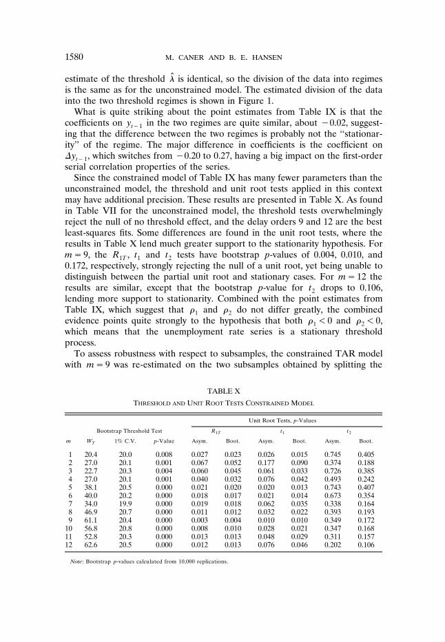
Since the constrained model of Table IX has many fewer parameters than theunconstrained model, the threshold and unit root tests applied in this contextmay have additional precision. These results are presented in Table X. As foundin Table VII for the unconstrained model, the threshold tests overwhelminglyreject the null of no threshold effect, and the delay orders 9 and 12 are the bestleast-squares fits. Some differences are found in the unit root tests, where theresults in Table X lend much greater support to the stationarity hypothesis. Form�9, the R , t and t tests have bootstrap p-values of 0.004, 0.010, and1T 1 20.172, respectively, strongly rejecting the null of a unit root, yet being unable todistinguish between the partial unit root and stationary cases. For m�12 theresults are similar, except that the bootstrap p-value for t drops to 0.106,2lending more support to stationarity. Combined with the point estimates fromTable IX, which suggest that and do not differ greatly, the combined1 2evidence points quite strongly to the hypothesis that both �0 and �0,1 2which means that the unemployment rate series is a stationary thresholdprocess.

To assess robustness with respect to subsamples, the constrained TAR modelwith m�9 was re-estimated on the two subsamples obtained by splitting the

TABLE X

THRESHOLD AND UNIT ROOT TESTS CONSTRAINED MODEL

Unit Root Tests, p-Values

Bootstrap Threshold Test R t t1T 1 2

m W 1% C.V. p-Value Asym. Boot. Asym. Boot. Asym. Boot.T

1 20.4 20.0 0.008 0.027 0.023 0.026 0.015 0.745 0.4052 27.0 20.1 0.001 0.067 0.052 0.177 0.090 0.374 0.1883 22.7 20.3 0.004 0.060 0.045 0.061 0.033 0.726 0.3854 27.0 20.1 0.001 0.040 0.032 0.076 0.042 0.493 0.2425 38.1 20.5 0.000 0.021 0.020 0.020 0.013 0.743 0.4076 40.0 20.2 0.000 0.018 0.017 0.021 0.014 0.673 0.3547 34.0 19.9 0.000 0.019 0.018 0.062 0.035 0.338 0.1648 46.9 20.7 0.000 0.011 0.012 0.032 0.022 0.393 0.1939 61.1 20.4 0.000 0.003 0.004 0.010 0.010 0.349 0.172

10 56.8 20.8 0.000 0.008 0.010 0.028 0.021 0.347 0.16811 52.8 20.3 0.000 0.013 0.013 0.048 0.029 0.311 0.15712 62.6 20.5 0.000 0.012 0.013 0.076 0.046 0.202 0.106



TABLE XI

SUBSAMPLE COMPARISONS, CONSTRAINED MODEL, m�9

First Half Sample Second Half Sample

� .479 .267 �.029 �.049ˆ1 �.033 �.031ˆ2� �.090 �.309ˆ1Ž1 .� .241 .165ˆ2Ž1 .

Ž .W p-value .000 .001TŽ .R p-value .167 .0131T

m 12 8ˆ


Ž .sample at its midpoint December, 1978 . The subsample estimates of theparameters �, , , and the first elements of � and � , denoted as � and1 2 1 2 1Ž1.� , respectively, are reported in Table XI. They appear7 to be remarkably2Ž1.stable across the two regimes. We also report the bootstrap p-values for thethreshold test W and the unit root test R . On each subsample, the thresholdT 1Ttest W easily rejects the null of linearity in favor of threshold nonlinearity. TheTunit root tests are split, with the first subsample failing to reject the nullhypothesis, while the null of a unit root is rejected in the second subsample.

We also assessed robustness with respect to alternative specifications of thedependent variable y . In our preferred model, the dependent variable is UR ,t tthe unemployment rate scaled to range from 0 to 100. By construction, thisvariable is bounded, and hence cannot strictly be a linear unit root process. It istempting to think that the boundary effect may bias our results, as the estimatedthreshold effect may be merely to incorporate this boundary condition. Toexplore this issue, we experimented with four transformations of the dependentvariable that are unbounded in either or both directions. The specific transfor-

Žmations and results are listed in Table XII. For each transformation setting

TABLE XII

SUMMARY RESULTS FOR ALTERNATIVE SPECIFICATIONS

UNCONSTRAINED MODEL

Dependent Variable ADF Statistic Log-Likelihood W p-Value R p-ValueT 1T

UR �2.40 174 0.000 0.029tŽ Ž ..log UR � 1�UR �2.41 161 0.000 0.078t tŽ .log UR �2.42 159 0.000 0.095t

Ž .�100 log 1�UR �100 �2.41 172 0.000 0.025tŽ Ž . .100 exp UR �100 �1 �2.41 172 0.000 0.026t


7 While it is tempting to attempt a formal test for parameter stability by comparing the estimatedparameters, we have no theory that is appropriate in this context and interpretation of the testscould be highly misleading.


. 8m�9 , the linear ADF statistic, Gaussian log-likelihood, and the bootstrapp-values for the W and R tests are reported. Two important results emerge.T 1T

First, none of the results are sensitive to the transformation selected. The linearADF statistic is virtually unchanged, and the p-values of the threshold tests areall overwhelmingly significant. The unit root tests yield minor differences, withsmall changes in the p-values across specifications. The differences, however,are not sufficient to alter our conclusions. Second, our preferred specificationŽ .which sets y �UR has the highest Gaussian log-likelihood. While we have not t

formal test to compare the models, the Gaussian log-likelihood is still a validmodel selection criteria, and its value certainly does not provide any evidenceagainst our preferred specification.

Furthermore, we explored the sensitivity of our results to the trimming region� � � � � � � �� , � . Our reported results set � , � � .15, .85 , but we also tried � , �1 2 1 2 1 2

� � � � � �� .10, .90 and � , � � .05, .95 . The point estimates are unchanged, and the1 2p-values for the threshold test statistics remain as reported. The only differencearises for the p-values for the unit root tests, which increase somewhat. Forexample, the bootstrap p-value for the R statistic rises from 0.029 to 0.035 to1T

0.043, for the three respective trimming regions. The model was also re-esti-mated adding a fitted linear time trend to each regime. None of the pointestimates or test statistics changed meaningfully, except that the unit root testswere reduced in statistical significance. For example the bootstrap p-value forthe R statistic rises to 0.103.1T

The stationarity of the post-war unemployment rate in a TAR model has alsoŽ .been recently explored by Tsay 1997 . His conclusions are quite similar to ours,

although his methods differ. His analysis is based on quarterly data over1948�1993, and uses a lagged first difference for the threshold variable. His unitroot test imposes the restriction � , and he compares his unit root t1 2statistic to the standard Dickey-Fuller distribution,9 while we base our infer-ences on a bootstrap distribution.

7. CONCLUSION

This paper developed a new asymptotic theory for threshold autoregressivemodels with a possible unit root. The joint application of the two tests�for athreshold and for a unit root�allows a researcher to distinguish nonlinear fromnonstationary processes. We illustrate the methods with an application to theU.S. unemployment rate, and find evidence to support the hypothesis that theprocess is a stationary nonlinear threshold autoregression.

8 Properly adjusted for the Jacobian of the transformation of the dependent variable.9 This is justified in Tsay’s paper only for the case of known threshold. An analog of our Theorem

7, however, shows that Tsay’s test with an estimated threshold continues to have the standardDickey-Fuller distribution under the auxiliary assumption that the threshold is identified.


It would be useful to generalize our analysis in several directions, includingŽ .multivariate models, multiple thresholds, and smooth threshold STAR models.

Such extensions may require different methods than those presented here.

Dept. of Economics, Uniersity of Pittsburgh, WW Posar Hall 4S01, Pittsburgh,PA 15260, U.S.A.; [email protected]

andDept. of Economics, Social Science Bldg., Uniersity of Wisconsin, Madison, WI

53706-1393, U.S.A.; [email protected]; http:��www.ssc.wisc.edu��bhansen�

Manuscript receied December, 1997; final reision receied July, 2000.

APPENDIX

2 � Ž . 4PROOF OF THEOREM 1: For simplicity, normalize � �1. For all u, 1 u e , � is a strictlyt�1 t tŽ Ž . 2 . Ž Ž ..stationary and ergodic MDS with variance E 1 u e �E 1 u �u. By the MDS central limitt�1 t t�1

Ž .theorem, for any s, u ,

� �Ts1Ž . Ž . Ž .Y s, u � 1 u e � N 0, su .ÝT t�1 t d'T t�1

Furthermore, the asymptotic covariance kernel is determined by

� � � �Ts � Ts1 212Ž Ž . Ž .. Ž Ž . Ž . .E Y s , u Y s , u � E 1 u 1 u eÝT 1 1 T 2 2 t�1 1 t�1 2 tT t�1

Ž .Ž .� s �s u �u .1 2 1 2

Combined with the Cramer-Wold device, this can be used to yield the convergence of the finitedimensional distributions.

Ž .The stochastic equicontinuity of Y s, u over � follows from that ofT

� �Ts1� Ž . Ž Ž . .Y s, u � 1 u �u e .ÝT t�1 t'T t�1

For any 0s �s 1 and 0u �u 1, let1 2 1 2

� � Ž . � Ž . � Ž . � Ž .Y *�Y s , u �Y s , u �Y s , u �Y s , uT T 2 2 T 1 2 T 2 1 T 1 1

� �Ts2�1 �2�T e aÝ t t�1

� �t� Ts1

Ž .where a �1 � u �u .t �u U � u 4 2 11 t 2

We show below that for any constant ��0 such that

� �Ž .A.1 u �u and s �s ,2 1 2 1T T

then

� �2�� 1Ž . � � � �Ž . Ž .A.2 E Y * K 1�� s �s u �uT 2 1 2 1


Ž .for K� and ��1�1�r. Bai 1996, Theorem A.1 established the stochastic equicontinuity of� Ž .Y s, u in a similar context. While he used a different set of dependence and moment bounds, aT

Ž .careful reading of his proof shows that these conditions are only used to prove inequality A.2Ž . Ž Ž . Ž .. Ž . Ž . Ž .under A.1 his equations 23 and 24 . Thus A.1 � A.2 are sufficient to establish that Y s, u isT

stochastically equicontinuous.Ž . Ž . Ž .We now prove A.2 under A.1 . First, from A.1 we deduce

Ž .1�r 1�1�r�1 �1Ž . Ž . Ž .A.3 T � s �s u �u2 1 2 1

Ž . Ž .��1 ��2�r�1 Ž . Ž .�� s �s u �u .2 1 2 1

Ž .Second, the uniform distribution of U Assumption 2.2 impliest�1

22� � Ž . Ž .E a �E 1 �21 u �u � u �uŽ .t�1 �u U � u 4 �u U � u 4 2 1 2 11 t 2 1 t 2

2Ž . Ž .Ž . Ž .� u �u �2 u �u u �u � u �u2 1 2 1 2 1 2 1

Ž . u �u .2 1

� � 2Since a 1, then for any ��2,t�1

Ž . � � � � � 2 Ž .A.4 E a E a u �u .t�1 t�1 2 1

� � 2 � � 2 � � r r�1Ž .Third, set q � a �E a and note that E q 2 u �u by the c inequality andt t�1 t�1 t 2 1 rŽ . � � 2 � � 2A.4 . Using the expansion a �E a �q , the c inequality, and Corollary 3 of Hansent�1 t�1 t rŽ . Ž .1991 which holds under Assumption 2.1 for some K �� , we find

2 2� � � �Ts Ts2 21 12 2Ž . � � Ž . � �A.5 E a �E s �s E a � qÝ Ýt�1 2 1 t�1 tT Tž / ž /� � � �t� Ts t� Ts1 1

2� �Ts212 2Ž . Ž .2 s �s u �u �2 E qÝ2 1 2 1 tT � �t� Ts1

2 K � 2� r2 2 rŽ . Ž . Ž .Ž � � .2 s �s u �u � s �s E q2 1 2 1 2 1 tT8 K �2 2 2�rŽ . Ž . Ž .Ž .2 s �s u �u � s �s u �u .2 1 2 1 2 1 2 1T

� 4 Ž Ž ..Finally, since e a , � is an MDS, by Rosenthal’s inequality Hall and Heyde 1980, p. 23 fort t�1 tŽ . Ž . Ž .some C� , Assumption 2.3, A.5 , A.4 , and A.3 ,

4� �Ts24� �1�2� �E Y * �E T e aÝT t t�1

� �t� Ts1

2� � � �Ts Ts2 21 12 4Ž � � � . � �C E E e a � � E e aÝ Ýt t�1 t�1 t t�12T Tž /� � � �t� Ts t� Ts1 1

2� �Ts21 2 4 4�1� � Ž . � � � ��C E a �T s �s E e E aÝ t�1 2 1 t t�1Tž /� �t� Ts1

2 2 2�r�1� Ž . Ž . Ž .Ž .C 2 s �s u �u �8T K � s �s u �u2 1 2 1 2 1 2 1

�1 Ž . Ž .��T s �s � u �u2 1 2 1

� ��1Ž .Ž . Ž .K 1�� s �s u �u2 1 2 1


Ž . Ž .2Ž .2 Ž .�Ž .�where K�C max 2, 8 K �� , using the fact that s �s u �u s �s u �u . This is2 1 2 1 2 1 2 1Ž .A.2 and completes the proof. Q.E.D.

Ž .PROOF OF THEOREM 2: For all u, Y s, u is a martingale with square integrable innovationsT�1 �1�2 Ž . Ž .� T 1 u e . For fixed u, Theorem 1 above and Theorem 2.2 in Kurtz and Protter 1991t�1 t

� �yield the stated result. Their result can be extended to the needed uniformity over u� 0, 1 as theirŽ .equation 1.13 holds uniformly in u, which can be verified using the bounded convergence theorem.

Q.E.D.

PROOF OF THEOREM 3: We prove part 1 under the weaker assumption that

Ž . � �1� � �2A.6 E w � .t

Parts 2 and 3 follow directly by redefinition of w and X .t T tŽ . Ž . Ž . Ž . Ž . T 1 Ž .Let u �1 u w �h u so that E u �0. Since 1�T Ý X �H X s ds by Assumptiont t t t t�1 T t 0

Ž .2.4 and the continuous mapping theorem CMT , it is sufficient to show that

T1Ž .sup X u � 0.Ý T t t pT0u1 t�1

� �Fix ��0 and let c�E w � . Observe thatt

Ž . � Ž . � � �A.7 sup u w �c.t t0u1

Ž .Since X s is continuous almost surely, there is some ��0 such that

Ž . � Ž . Ž . �A.8 P 2c sup X s �X s� � �1�� .ž /� �s�s� �

� � � � � Ž .Set N� 1�� , and for k�0, . . . , N�1 set t � kT� �1 and t � t �1. By A.7 , the Ergodick k k�1Theorem, Assumption 2.4, and the CMT,

t�N�1 Tk1 1

Ž . � � � Ž . � � � � Ž . �A.9 X �X sup u sup X �X sup uÝ Ý ÝT t T t t T t T t � tkT T0u1 � � 0u1t�t � T�k�0 t�t t�1k

T1� � Ž � � . sup X �X w �cÝT t T t � tž /T� �t�t � T� t�1

� Ž . Ž . ��2c sup X s �X s� .� �s�s� �

Ž .Lemma 1 of Hansen 1996 states that

N1Ž . Ž .A.10 V � sup u � 0.ÝN t pN0u1 t�1

1 1� � �2NŽ . � � � � Ž .Since A.7 implies that V Ý w �c, and E w � by A.6 , it follows that V isN t�1 t t NNŽ . Ž .uniformly integrable. Theorem 25.12 of Billingsley 1986 states that uniform integrability and A.10

imply EV �0. This impliesN� �t tN�1 k k1 1

Ž . Ž .E sup u �E sup u �EV �0Ý Ý Ýt t T�T T�0u1 0u1k�0 t�t t�tk k

as T� , which implies�tN�1 k1

Ž . Ž .A.11 sup u � 0Ý Ý t pT 0u1k�0 t�tk


Ž . Ž . Ž .by Markov’s inequality. A.9 , A.11 and the fact that X �O 1 uniformly in t implyT t p

�tT N�1 k1 1Ž . Ž .sup X u � sup X uÝ Ý ÝT t t T t tT T0u1 0u1t�1 k�0 t�tk

�tN�1 k1� � Ž . sup X sup uÝ ÝT t tT1tT 0u1k�0 t�tk

t�N�1 k1

� � � Ž . �� X �X sup uÝ Ý T t T t tkT 0u1k�0 t�tk

� Ž . Ž . ��2c sup X s �X s�� s�s� �

�

Ž .where the last inequality holds with probability exceeding 1�� by A.8 . This establishes the result.Q.E.D.

Ž . � �PROOF OF THEOREM 4: Set U �G Z �U 0, 1 . Due to the equality 1 �1 , thet t �Z � �4 �U � G Ž�.4t�1 t�1Ž .change-of-variables u�G � allows us to re-write the test statistic as

� Ž .W � sup W u ,T T� �u� � , �1 2

� Ž .where W u is the Wald statistic for the equality of � �� in the regressionT 1 2

Ž . � �A.12 � y �x � 1 �x � 1 �e .t t�1 1 �U � u4 t�1 2 �U � u4 tt�1 t�1

Define

T

1 wÝ �U � u4 t�1t�1t�1Ž .w u �w �1 t�1 t�1 T

1Ý �U � u4t�1t�1

and

T

1 wÝ �U � u4 t�1t�1t�1Ž .w u �w � ,2 t�1 t�1 T

1Ý �U � u4t�1t�1

which is w projected orthogonal to 1 and 1 , respectively. Since the interceptst�1 �U � u4 �U � u4t�1 t�1Ž .1 and 1 are included in the regression A.12 , we can replace w 1 and�U � u4 �U � u4 t�1 �U � u4t�1 t�1 t�1

Ž . Ž .w 1 by w u 1 and w u 1 , respectively, without affecting the testt�1 �U � u4 1 t�1 �U � u4 2 t�1 �U � u4t�1 t�1 t�1� Ž . � Ž .statistic W u . We can also rescale y and t without affecting the value of W u , so that theT t�1 Tlatter can be calculated as the Wald statistic from the regression

Ž � Ž . . Ž � Ž . .� y � X w u � � 1 � X w u � � 1 �e ,t T t�1 1 t�1 1 �U � u4 T t�1 2 t�1 2 �U � u4 tt�1 t�1

where

yt�1 �Ž .X � � r � .T t�1 T t1�2ž /Ž .��a T


Ž .Now define 1 u �1 . Assumptions 2.1, 2.2, 2.3, and 2.4 are directly implied byt�1 �U � u4t�1

Assumption 1, so Theorem 1 yields

� �Ts1Ž . Ž . Ž .A.13 1 u e �W s, u ,Ý t�1 t'� T t�1

Ž .where W s, u is a two-parameter Brownian motion. Furthermore,

T1Ž . Ž . Ž .A.14 1 u w e �W u ,Ý t�1 t�1 t 2'� T t�1

Ž .where W u is a mean-zero vector Gaussian process with kernel2

Ž Ž . Ž . . Ž .E W u W u � �H u �u ,2 1 2 2 1 2

Ž . Ž . Ž .by Theorem 1 of Hansen 1996 . Furthermore, equations A.13 � A.14 hold jointly. Namely, theŽ . Ž .processes W s, u and W u are jointly Gaussian with covariance kernel2

Ž Ž . Ž .. Ž .E W u W s, u �h u �u .2 1 2 1 2

The convergence of the joint finite dimensional distributions may be obtained by the MDS centralŽ . Ž .limit theorem and the Cramer-Wold device. Stochastic equicontinuity follows from A.13 and A.14

Žand the fact that our convergence is in respect to the uniform metric since the limit processes are.continuous .

The inclusion of the intercept and trend variables in the regression means that the test statistic� Ž .W u is invariant to the actual value of �. We can thus without loss of generality set ��0. UnderT

Ž . Ž .H we see that y is generated by the stochastic process a L � y �e where a L is a lag0 t t tŽ . Ž .polynomial satisfying a 1 �a�1�� t. As a consequence of A.13 ,

� �Ts1Ž . Ž .e �W s, 1 �W sÝ t'� T t�1

and

Ž . �1 �2 Ž . Ž .A.15 T y � ��a W s .�T s �

Ž . Ž Ž . Ž . .It follows that X �X s � W s r s � �, establishing Assumption 2.4.T �T s �� Ž .Standard algebra shows that W u can be written asT

�1�1� �Ž . Ž Ž . Ž . Ž . Ž .. Ž .S u � M u �M u M 1 M u S uT T T T T T� Ž .W u � ,T 2 2Ž .� u ��ˆ

� Ž . Ž . Ž . Ž .�1 Ž .where S u �S u �M u M 1 S 1 ,T T T T T

Ž .S u1TŽ .S u �T Ž .ž /S u2T

T1Ž .1 u X eÝ t�1 T t�1 t'� T t�1� ,T1

Ž . Ž .1 u w u e� 0Ý t�1 1 t�1 t'� T t�1


and

Ž . Ž .M u M u �11T 21TŽ .M u �T Ž . Ž .ž /M u M u21T 22T

T T1 1�Ž . Ž . Ž .1 u X X 1 u X w u �Ý Ýt�1 T t�1 T t�1 t�1 T t�1 1 t�1T Tt�1 t�1� .T T1 1

�Ž . Ž . Ž . Ž . Ž .1 u w u X 1 u w u w u �� 0Ý Ýt�1 1 t�1 T t�1 t�1 1 t�1 1 t�1T Tt�1 t�1

Theorem 3 yields

1Ž . Ž . Ž .M u �u X s X s �ds,H11T0

T

Ž .1 u wÝ t�1 t�1T T1 1 t�1� �Ž . Ž . Ž .M u � 1 u w X � 1 u XÝ Ý21T t�1 t�1 T t�1 t�1 T t�1TT Tt�1 t�1Ž .1 uÝ t�1t�1

Ž .h u1 1Ž . Ž . Ž .�h u X s �ds� u X s �ds�0,H Hu0 0

and

T T�Ž . Ž .1 u w 1 u wÝ Ýt�1 t�1 t�1 t�1T1 t�1 t�1�Ž . Ž .M u � 1 u w w �Ý22 T t�1 t�1 t�1 TT t�1 Ž .1 uÝ t�1

t�1

Ž . Ž .h u h u �Ž . Ž .�H u � �� u .

u

Ž .Hence M u is asymptotically block-diagonal. It follows thatT

�1�1� � �Ž . Ž . Ž Ž . Ž . Ž . Ž .. Ž .W u �S u � M u �M u M 1 M u S uT 1T 11T 11T 11T 11T 1T

�1�1� �Ž . Ž Ž . Ž . Ž . Ž .. Ž . Ž .�S u � M u �M u M 1 M u S u �o 1 ,2T 22T 22T 22T 22T 2T p

where

�1� Ž . Ž . Ž . Ž . Ž .S u �S u �M u M 1 S 11T 1T 11T 11T 1T

and

�1� Ž . Ž . Ž . Ž . Ž .S u �S u �M u M 1 S 1 .2T 2T 22T 22T 2T

Theorem 2 yields

1Ž . Ž . Ž . Ž .S u � X s dW s, u ��J u ,H1T 10

and

�11 1� �Ž . Ž . Ž . Ž . Ž . Ž . Ž . Ž .S u �J u �u X s X s �ds X s X s �ds J 1 �J u .H H1T 1 1 1ž / ž /0 0


Ž .A.13 implies

T

Ž .1 u wÝ t�1 t�1T T1 1 t�1Ž . Ž . Ž .S u � 1 u w e � 1 u eÝ Ý2T t�1 t�1 t t�1 tT' '� T � Tt�1 t�1Ž .1 uÝ t�1t�1

Ž .h uŽ . Ž . Ž .�W u � W u �J u ,2 2u

and�1� Ž . Ž . Ž . Ž . Ž .S u �J u �� u � 1 J 1 .2T 2 1

Ž . Ž .Observe that J u is a Gaussian process with kernel � u . To see this, note that if u u ,2 1 2

Ž . Ž .h u h u1 2Ž Ž . Ž . . Ž . Ž . Ž . Ž .E J u J u � �E W u � W u W u � W u2 1 2 2 2 1 1 2 2 2ž / ž /ž /u u1 2

Ž . Ž . Ž . Ž .h u h u � h u h u �1 2 1 2Ž . Ž . Ž .�H u � h u ��h u � u1 1 1 1u u u u1 2 1 2

Ž . Ž .h u h u �1 1Ž . Ž .�H u � �� u .1 1u1

Ž . Ž .Also, J u is independent of W s, u , since they are Gaussian and orthogonal:2

Ž .h uŽ Ž . Ž .. Ž Ž . Ž .. Ž Ž . Ž ..E J u W s, u �E W u W s, u � E W u W s, u2 2 2u

Ž .h uŽ .�h u s� su�0.

u

It follows that J and J are independent processes.1 2Together, we find that

�11� �Ž . Ž . Ž . Ž .J u � X s X s �ds J uH1 1ž /0� Ž .W u �T Ž .u 1�u

�1�1� �Ž . Ž Ž . Ž . Ž . Ž .. Ž .� J u � � u �� u � 1 � u J u2 2

Ž . Ž . Ž .�Q u �Q u �T u .1 2

We conclude that� Ž . Ž .W � sup W u � sup T u ,T T

� � � �u� � , � u� � , �1 2 1 2

which is the stated result. Q.E.D.

PROOF OF THEOREM 5: Since the regression includes a trend, the test statistic is invariant to theintercept �� , so we set ��0 to ease exposition. We reparameterize the model as in1 2Ž . Ž . Ž .A.12 , letting u�G � . Standard algebraic results for linear regression show that t � t u andˆ1 1

Ž . Ž . Ž . Ž . Ž . Ž .t � t u where t u and t u are the t ratios for u and u in equation A.12 with u fixed,ˆ ˆ ˆ2 2 1 2 1 2and

� Ž .u� argmax W uˆ T� �u� � , �1 2


� Ž . Ž .where W u is defined before A.12 . To find the limit distribution of R , we find the limitT TŽ . Ž .distributions of t u and t u considered as a function of u, find the limit distribution of u, andˆ1 2

combine these results with the continuous mapping theorem.Ž . Ž . Ž .Let r � � r � and set w u as in the proof of Theorem 4. We can write t u explicitly asT t T t 1 t�1 1

� Ž .N uTŽ . Ž .A.16 t u � ,1 1�2� 2Ž Ž . Ž ..D u � uˆT

where

�1� Ž . Ž . Ž . Ž . Ž .N u �N u �B u �C u G u ,T T T T T

�1� Ž . Ž . Ž . Ž . Ž .D u �D u �B u �C u B u ,T T T T T

T1Ž . Ž .N u � y e 1 u ,ÝT t�1 t t�1T t�1

T12Ž . Ž .D u � y 1 u ,ÝT t�1 t�12T t�1

T1Ž .r y 1 uÝ T t t�1 t�13�2T t�1Ž .B u � ,T T1

Ž . Ž .w u y 1 uÝ 1 t�1 t�1 t�13�2T t�1

T T1 1� Ž . Ž . Ž .r r 1 u r w u �1 uÝ ÝT t T t t�1 T t 1 t�1 t�1T Tt�1 t�1Ž .C u � ,T T T1 1

�Ž . Ž . Ž . Ž . Ž .w u r 1 u w u w u �1 uÝ Ý1 t�1 T t t�1 1 t�1 1 t�1 t�1T Tt�1 t�1

and

T1Ž .r e 1 uÝ T t t t�11�2T t�1Ž .G u � .T T1

Ž . Ž .w u e 1 uÝ 1 t�1 t t�11�2T t�1

Ž . Ž . Ž . Ž .From A.15 we see that y � ��a W s . Also, note that r � r s . Hence�T r � T �T s �

12Ž . Ž . Ž . Ž .N u � � �a W s dW s, u ,HT0

1 22 2Ž . Ž . Ž .D u � � �a W s ds,HT0

1Ž . Ž . Ž .��a u r s W s dsHŽ .B u � ,0T

0

1 Ž . Ž .u r s r s �ds 0HŽ .C u � ,0T

Ž .0 � u


and

1 Ž . Ž .� r s dW s, uHŽ .G u � .0TŽ .� J u2

� Ž . Ž 2 . 1 Ž . Ž . Ž .Thus N u � � �a H W * s dW s, u , where W * s is detrended Brownian motion as definedT 0� Ž . Ž 2 2 . 1 Ž .2in the statement of Theorem 5. Similarly, D u � � �a H W * s ds. It follows thatT 0

1 Ž . Ž .H W * s dW s, u0Ž . Ž . Ž .A.17 t u � � t u .1 11�221Ž Ž . .uH W * s ds0

Using similar arguments, we can show that

� 1 Ž .Ž Ž . Ž ..�H W * s dW s, 1 �dW s, u0Ž . Ž . Ž .A.18 t u � � t u ,2 21�221ŽŽ . Ž . .1�u H W * s ds0

Ž . Ž . Ž . Ž .and A.17 and A.18 hold jointly. Theorem 2 shows that t u and t u are continuous functions of1 2Ž .u almost surely .

� Ž . Ž .Finally, we need the limit distribution of u. In Theorem 4 we showed that W u �T u . Thisˆ TŽ . � �limit process T u is continuous in u and has a unique maximum in � , � with probability one.1 2

Ž .This allows the application of Theorem 2.7 of Kim and Pollard 1990 ; hence

Ž . � Ž . Ž .A.19 u� argmax W u � argmax T u �u*.ˆ T� � � �u� � , � u� � , �1 2 1 2

Ž . Ž . Ž .Equation A.17 , A.18 , and A.19 combine to yield the first statement of the theorem:

Ž . Ž Ž . Ž ..t , t � t u* , t u* .1 2 1 2

Ž .The convergence of R follows from the continuity of R �,� and the continuous mapping theorem.TQ.E.D.

Ž .PROOF OF THEOREM 6: As in the previous proof we use the reparameterized model A.12 whereˆ 2 2Ž . Ž . Ž .u�G � , u�G � , and u �G � . Since the test statistic is invariant to � , we set � �1.ˆ 0 0

Ž . Ž . Ž . Ž . Ž .As in the prior proof, t � t u and t � t u . Consider t u . For u�u , t u is given by A.16 .ˆ ˆ1 1 2 2 1 0 1For u�u , note that0

� y �� x 1 �� x 1 �et 1 t�1 �U � u 4 2 t�1 �U � u 4 tt�1 0 t�1 0

�� x 1 �� x 11 t�1 �U � u4 2 t�1 �U � u4t�1 t�1

ŽŽ . Ž . .� � �� w 1 �e ,2 1 2 1 t�1 �u U � u4 t0 t�1

so by linear projection,

� Ž . Ž .N u �A uT TŽ . Ž .A.20 t u � ,1 1�2� 2Ž Ž . Ž ..D u � uˆT

� Ž . � Ž . Ž .where N u and D u are defined below A.16 ,T T

T1��Ž . Ž . �Ž . Ž .�A u � y u � �� w � �� 1 ,ÝT t�1 2 1 t�1 2 1 �u U � u40 t�1T t�1

�� Ž .and y u is y 1 projected orthogonal to the other regressors.t�1 t�1 �U � u4t�1


Ž .We now show that A u � 0. LetˆT p

Ž . � Ž .� � � �� w � �� ,t 2 1 t�1 2 1

Ž . Ž .� u �E � 1t �u U � u40 t�1

Ž .Ž . Ž . Ž Ž . Ž ..� � �� u�u � � �� h u �h u ,2 1 0 2 1 0

and

T1Ž . Ž Ž ..G u � � 1 �� u .ÝT t �u U � u40 t�1'T t�1

Then

T1 1��Ž . � Ž . �A u max y u � 1ÝT t�1 t �u U � u40 t�1' 'tTT T t�1

'Ž . � Ž . Ž .�O 1 � G u � T � u ,p T

'Ž . Ž .uniformly in u. We complete the claim by next showing that G u � 0 and T � u � 0.ˆ ˆT p pŽ . Ž . Ž .In the context of an identified ergodic TAR, Chan 1993 has shown that T u�u �O 1 , andˆ 0 p

10 Ž .his proof extends to the present model. The empirical process G u satisfies the conditions ofTŽ . Ž . Ž .Theorem 1, application 4, of Doukhan, Massart, and Rio 1995 , so G u �G u , a GaussianT

Ž . Ž .process with continuous sample paths. As u� u , it follows that G u �G u �0. Since e hasˆ ˆp 0 T 0 tŽ � .a continuous distribution, E w U �u is continuous in u, so is bounded in the neighborhoodt�1 t�1

of u . Thus0

d dŽ . Ž . Ž . Ž .� u � � �� h u2 1 2 1du du

Ž . Ž . Ž � .� � �� E w U �u2 1 2 1 t�1 t�1

is bounded in this neighborhood, and hence

d' ' '� Ž . � � Ž . Ž . � Ž . � � Ž .T � u � T � u �� u � u T u�u �o 1 .ˆ ˆ ˆ ˆ0 0 pdu

Ž .We conclude that A u � 0 as desired.ˆT pŽ .Combined with A.20 , it follows that

� Ž .N uTŽ . Ž .t u � �o 1 .ˆ1 p1�2� 2Ž Ž . Ž ..D u � uˆ ˆ ˆT

2 Ž .Let � be defined as 12 , and as noted before the statement of Theorem 6, � y is zero-mean,y tstrictly stationary and geometrically ergodic. An extension of Theorem 1 is the joint convergence

Ž . � �2over s, u � 0, 1 :

� �Ts1Ž .e 1 uÝ t t�1'T Ž .t�1 W s, u�� Ts Ž .W sž /1 3

� yÝ t� 0'� Ty t�1

10 This extension is available on request from the authors.


Ž 2 2 . Ž .recall that we have set Ee �� 1 , where W s, u is a two-parameter Brownian motion and Wt 3is a standard Brownian motion. This implies

� �Ts� �1e 1Ý t �U � u 4t�1 0'u T' 0 t�1

Ž .W s� � 1Ts1Ž . Ž .e 1 W s� �W sÝ t �U � u 4 2t�1 0'1�u T' 0 t�1 � 0Ž .W s3

� �Ts1� yÝ t� �'� Ty t�1

where alternative expressions are

Ž .W s, u0Ž .W s � ,1 u' 0

Ž . Ž .W s, 1 �W s, u0Ž .W s � .2 1�u' 0

Ž .By construction, the vector Brownian motion W s has covariance matrix

1 0 �1

Ž . Ž . Ž . 0 1 �A.21 EW 1 W 1 �� ,2� 0� � 11 2

Ž . Ž .where � and � are defined in 13 and 14 . These results imply that1 2

1Ž .y �� W s .�T s � y 3'T

Using an arguments identical to that of the previous proof, we see that

1 2� �2Ž . Ž .D u �u� W s dsHT y 30

and

1� �Ž . Ž . Ž .N u �� W s dW s, uHT y 30

� Ž . Ž . 1 Ž . Ž . Ž 1 Ž . Ž . .�1 Ž .where W s �W s �H W a r a �da H r a r a �da r s .3 3 0 3 0Since these limits are continuous in u almost surely and u� u , it follows thatˆ p 0

1 � Ž . Ž .� W s dW s, uHy 3 00Ž . Ž .A.22 t � t u �ˆ1 1 1�22�2 1 Ž .u � H W s dsŽ .0 y 0 3

1 � Ž . Ž .W s dW sH 3 10� .1�2

1 2� Ž .W s dsH 3ž /0

Similar arguments yield

1 � Ž . Ž .W s dW sH 3 20Ž .A.23 t � .2 1�2

1 2� Ž .W s dsH 3ž /0


Ž . 11Using A.21 we can write

1�22Ž . Ž . Ž .W s 1�� W s �1 1 1�3 1Ž . Ž .A.24 � � W s ,31�2 �Ž . ž /ž / 2W s 2ž /2 Ž . Ž .1�� W s2 2 �3

Ž .where W , W � is independent of W and has covariance matrix1�3 2 �3 3

1 �21 ,� 1ž /21

Ž . Ž . Ž .where � is defined in 16 . From A.22 � A.24 we find that21

1 1� �Ž . Ž . Ž . Ž .W s dW s W s dW sH H3 1�3 3 31�2 0 02Ž .t � 1�� 1 1 11�2 1�2

1 12 2� �Ž . Ž .W s ds W s dsH H3 3ž / ž /0 0

and

1 1� �Ž . Ž . Ž . Ž .W s dW s W s dW sH H3 2 �3 3 31�2 0 02Ž .t � 1�� ,2 2 21�2 1�2

1 12 2� �Ž . Ž .W s ds W s dsH H3 3ž / ž /0 0

which can be written as

1�22Ž .1�� Zt �1 11 1Ž . ˆA.25 t� � � DF1�2t �ž / ž /22 2ž /Ž .1�� Z2 2

Ž . Ž .where Z , Z has distribution 15 and is independent of DF. This establishes the first stated result1 2of the theorem.

Now set

� �a �� a1 2H�� a � �až /2 1

Ž . Ž .where a is defined in 17 , and note that H�H�I. Then some algebraic manipulations and A.25show that

1�22Ž .1�� Z �1 1 1ˆH�t�H� �H� DF1�2 �ž /2 2ž /Ž .1�� Z2 2

N1 a� � DFž /N 0ž /2

11 The derivation is straightforward, yet cumbersome, so is omitted; it can be obtained on requestfrom the authors.


Ž 2 . Ž .where N �N 0, 1�a , N �N 0, 1 , and DF are mutually independent. Hence since HH��I,1 2

R � t 2 � t 22T 1 2

ˆˆ� t�t

ˆ ˆ� t�HH�t

N N�1 1a a� � DF � DFž / ž /N 0 N 0ž / ž /2 2

2 2Ž .� N �aDF �N ,1 2

Ž 2 .�1 �2 2 2which is the final statement of the theorem, setting Z� 1�a N and � �N . Q.E.D.1 1 2

REFERENCES

Ž .ALTISSIMO, F., AND G. VIOLANTE 1996 : ‘‘Persistence and Nonlinearity in U.S. GNP and Unemploy-ment: An Endogenous Delay Threshold VAR,’’ University of Pennsylvania.

Ž .ANDREWS, D. W. K. 1993 : ‘‘Tests for Parameter Instability and Structural Change with UnknownChange Point,’’ Econometrica, 61, 821�856.

Ž .�� 1998 : ‘‘Hypothesis Testing with a Restricted Parameter Space,’’ Journal of Econometrics, 84,155�199.

Ž .ANDREWS, D. W. K., AND W. PLOBERGER 1994 : ‘‘Optimal Tests when a Nuisance Parameter isPresent only under the Alternative,’’ Econometrica, 62, 1383�1414.

Ž .BAI, J. 1996 : ‘‘Testing for Parameter Constancy in Linear Regressions: An Empirical DistributionFunction Approach,’’ Econometrica, 64, 597�622.

Ž .BALKE, N. S., AND T. B. FOMBY 1997 : ‘‘Threshold Cointegration,’’ International Economic Reiew,38, 627�645.

Ž .BEAUDRY, P., AND G. KOOP 1993 : ‘‘Do Recessions Permanently Change Output?’’ Journal ofMonetary Economics, 31, 149�164.

Ž .BILLINGSLEY, P. 1986 : Probability and Measure, 2nd Ed. New York: Wiley.Ž .CHAN, K. S. 1991 : ‘‘Percentage Points of Likelihood Ratio Tests for Threshold Autoregression,’’

Journal of the Royal Statistical Society, Series B, 53, 691�696.Ž .�� 1993 : ‘‘Consistency and Limiting Distribution of the Least Squares Estimator of a

Threshold Autoregressive Model,’’ The Annals of Statistics, 21, 520�533.Ž .CHAN, K. S., AND H. TONG 1985 : ‘‘On the Use of the Deterministic Lyapunov Function for the

Ergodicity of Stochastic Difference Equations,’’ Adances in Applied Probability, 17, 667�678.Ž .CHAN, K. S., AND R. S. TSAY 1998 : ‘‘Limiting Properties of the Least Squares Estimator of a

Continuous Threshold Autoregressive Model,’’ Biometrika, 45, 413�426.Ž .CHEN, C. W. S., AND J. C. LEE 1995 : ‘‘Bayesian Inference of Threshold Autoregressive Models,’’

Journal of Time Series Analysis, 16, 483�492.Ž .DAVIES, R. B. 1987 : ‘‘Hypothesis Testing when a Nuisance Parameter is Present only under the

Alternative,’’ Biometrika, 74, 33�43.Ž .DICKEY, D. A., AND W. A. FULLER 1979 : ‘‘Distribution of the Estimators for Autoregressive Time

Series with a Unit Root,’’ Journal of the American Statistical Association, 74, 427�431.Ž .DOUKHAN, P., P. MASSART, AND E. RIO 1995 : ‘‘Invariance Principles for Absolutely Regular

Empirical Processes,’’ Annales de l’Institut Henri Poincare, 31, 393�427.Ž .GALBRAITH, J. W. 1996 : ‘‘Credit Rationing and Threshold Effects in the Relation between Money

and Output,’’ Journal of Applied Econometrics, 11, 419�429.Ž .GINE, E., AND J. ZINN 1990 : ‘‘Bootstrapping General Empirical Measures,’’ The Annals of

Probability, 18, 851�869.Ž .GONZALEZ, M., AND J. GONZALO 1998 : ‘‘Threshold Unit Root Models,’’ U. Carlos II de Madrid.

Ž .HALL, P., AND C. C. HEYDE 1980 : Martingale Limit Theory and Its Application. New York: AcademicPress.


Ž .HAMILTON, J. 1989 : ‘‘A New Approach to the Economic Analysis of Nonstationary Time Series andthe Business Cycle,’’ Econometrica, 5, 357�384.

Ž .HANSEN, B. E. 1991 : ‘‘Strong Laws for Dependent Heterogeneous Processes,’’ Econometric Theory,7, 213�221.

Ž .�� 1992 : ‘‘Convergence to Stochastic Integrals for Dependent Heterogeneous Processes,’’Econometric Theory, 8, 489�500.

Ž .�� 1996 : ‘‘Inference when a Nuisance Parameter is not Identified under the Null Hypothesis,’’Econometrica, 64, 413�430.

Ž .�� 1997a : ‘‘Approximate Asymptotic p-Values for Structural Change Tests,’’ Journal ofBusiness and Economic Statistics, 15, 60�67.

Ž .�� 1997b : ‘‘Inference in TAR Models,’’ Studies in Nonlinear Dynamics and Econometrics, 1,119�131.

Ž .�� 2000 : ‘‘Sample Splitting and Threshold Estimation,’’ Econometrica, 68, 575�603.Ž .KIM, J., AND D. POLLARD 1990 : ‘‘Cube Root Asymptotics,’’ The Annals of Statistics, 18, 191�219.

Ž .KURTZ, T. G., AND P. PROTTER 1991 : ‘‘Weak Limit Theorems for Stochastic Integrals andStochastic Differential Equations,’’ The Annals of Probability, 19, 1035�1070.

Ž .MONTGOMERY, A. L., V. ZARNOWITZ, R. S. TSAY, AND G. C. TIAO 1998 : ‘‘Forecasting the U.S.Unemployment Rate,’’ Journal of the American Statistical Association, 93, 478�493.

Ž .NEFTCI, S. 1984 : ‘‘Are Economic Time Series Asymmetric over the Business Cycle?’’ Journal ofPolitical Economy, 92, 307�328.

Ž .PHAM, T. D., AND L. T. TRAN 1985 : ‘‘Some Mixing Properties of Time Series Models,’’ StochasticProcesses and Their Applications, 19, 297�303.

Ž .PIPPENGER, M. K., AND G. E. GOERING 1993 : ‘‘A Note on the Empirical Power of Unit Root Testsunder Threshold Processes,’’ Oxford Bulletin of Economics and Statistics, 55, 473�481.

Ž .POTTER, S. M. 1995 : ‘‘A Nonlinear Approach to U.S. GNP,’’ Journal of Applied Econometrics, 2,109�125.

Ž .ROTHMAN, P. 1991 : ‘‘Further Evidence on the Asymmetric Behavior of Unemployment Rates overthe Business Cycle,’’ Journal of Macroeconomics, 13, 291�298.

Ž .SAID, S. E., AND D. A. DICKEY 1984 : ‘‘Testing for Unit Roots in Autoregressive-Moving AverageModels of Unknown Order,’’ Biometrika, 71, 599�608.

Ž .TONG, H. 1978 : ‘‘On a Threshold Model,’’ in Pattern Recognition and Signal Processing, ed. by C. H.Chen. Amsterdam: Sijhoff and Noordhoff.

Ž .�� 1983 : Threshold Models in Non-linear Time Series Analysis. Lecture Notes in Statistics, 21.Berlin: Springer.

Ž .�� 1990 : Non-Linear Time Series: A Dynamical System Approach. Oxford: Oxford UniversityPress.

Ž .TSAY, R. S. 1997 : ‘‘Unit-root Tests with Threshold Innovations,’’ University of Chicago.

Econometrica, Vol. 69, No. 6 November, 2001 , 1555 1596bhansen/papers/ecnmt_01.pdf ·...

Documents

Transcript of Econometrica, Vol. 69, No. 6 November, 2001 , 1555 1596bhansen/papers/ecnmt_01.pdf ·...