8/18/2019 ECE6323_S16_HW3

http://slidepdf.com/reader/full/ece6323s16hw3 1/2

ECE 6323 - HW 3U of Houston Han Le - Copyrighted

Loss in fiber

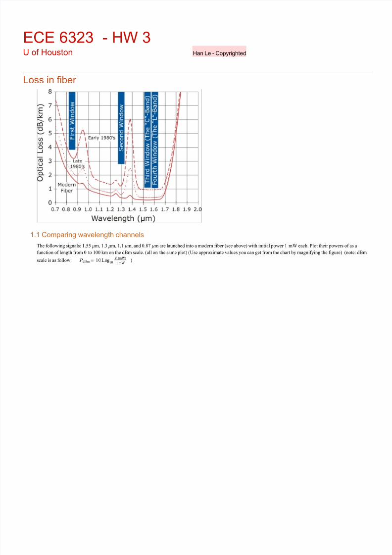
1.1 Comparing wavelength channels

The following signals: 1.55  mm, 1.3  mm, 1.1  mm, and 0.87  mm are launched into a modern fiber (see above) with initial power 1 mW each. Plot their powers of as a

function of length from 0 to 100 km on the dBm scale. (all on the same plot) (Use approximate values you can get from the chart by magnifying the figure) (note: dBm

scale is as follow:  P dBm  = 10 Log10

 P  HmWL1 mW

  )

8/18/2019 ECE6323_S16_HW3

http://slidepdf.com/reader/full/ece6323s16hw3 2/2

1.2 Comparing channels - part 2

Do the same as 1.1, but in terms of number of photons on log 10 scale.

1.3 Let the signals now be Gaussian pulses

Let the pulse have a power envelope ã-2 z 

2‘s2

, where s=10 ps. As the pulse travels, it also suffers back scattering which means that some of the light is scattered back-

ward, opposite to the direction of its travel. The scattering was both from intrinsic mechanism and extrinsic causes such as fiber structure imperfection.

Let 2 Gaussian pulses of 1.55  mm and 1.3  mm be launched into a 10-km fiber, joined with another segment of 15-km fiber, with a 3-dB reflection at the fiber joint.

Plot the relative intensity of backscattered light on dB scale as a function of time (over the roundtrip time-of-flight in the f ibre). Make also a plot just around the time

when the pulses are passing the fiber joint.

Assume that the group velocity effective index is 1.46 for 1.55  mm and 1.47 for 1.3  mm. Assume that there is no reflection at the end facet of the whole fiber.

Hint: see discussion of OTDR below.

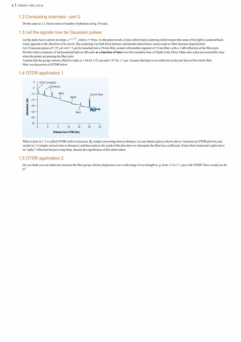
1.4 OTDR application 1

 

What is done in 1.3 is called OTDR (refer to lectures). By simply converting time-to-distance, we can obtain a plot as shown above. Generate an OTDR plot for your

results in 1.3 (simply convert time to distance), and then analyze the result of the plot above to determine the fiber loss coefficient. Notice that a bend and a splice have

no “spiky” reflection but just a step drop, discuss the significance of this observation.

1.5 OTDR application 2

Do you think you can indirectly measure the fiber group velocity dispersion over a wide range of wavelength (e. g. from 1.3 to 1.7  mm) with OTDR? How would you do

it?

2   ECE6323 -HW3_S16.nb