ECE1724 Project Report: ECE1724 ProjectSpeeded-Up Speeded...

ECE1724 Project ReportRev: 1.0

April 18, 2009

ECE1724 ProjectSpeeded-Up Speeded-Up Robust Features

Paul Furgale, Chi Hay Tong, and Gaetan Kenway<[email protected]><[email protected]><[email protected]>

1 Introduction

Feature detection and matching is one of the fundamental problems in low-level computer vision. Given a series ofimages of the same object, feature detection and matching algorithms try to (1) repeatably detect the same point ofinterest in every image, regardless of the scale and orientation of the object, (2) match each point of interest from oneimage with the same point in another image. Feature detection and matching form the basis for many higher-levelalgorithms such as object recognition [1], robot navigation [2], panorama stitching [3], and three-dimensional scenemodeling [4].

In the last 10 years, the Scale Invariant Feature Transform (SIFT) [5] has become the standard algorithm forthis task. However, while its performance is quite impressive on difficult matching tasks, it is too computationallyexpensive to use in online or real-time applications. In response to this, Bay et al. proposed the Speeded-UpRobust Feature (SURF) [6], which uses an integral image (essentially a 2D prefix sum) to approximate many of thecalculations in the SIFT algorithm. The SURF algorithm is much faster than SIFT, but it is still not fast enough touse in real-time applications.

Our interest is the use of the SURF algorithm for real-time robot navigation. Traditionally, visual motion esti-


April 18, 2009

mation has used more efficient, less robust algorithms for this task (e.g. [7, 8]). However, with the introduction ofefficient numerical methods that estimate the motion of a vehicle using features tracked over multiple frames [8],we believe that using a better feature detection and matching algorithm should (1) increase the accuracy of visualmotion estimation, and (2) allow robots to determine their unique location within a map of visual features. SURFis much faster to compute than SIFT (interestingly, SURF is about as fast as GPU-accelerated SIFT), but it is stillnot fast enough to use in real-time. Therefore, it was our goal to use the GPU to accelerate the SURF algorithm to apoint that it may be used in real-time robot navigation.

Rather than choosing a very simple algorithm and optimizing it as far as it could go, we have implemented whatended up being a very complicated algorithm. We were first and foremost concerned with verifying that the algorithmwas correct, and second to that, optimization. To do this, we had to verify that the algorithm implemented on theCPU matched the original paper as closely as possible. Then we checked that each part of our GPU implementationmatched the CPU implementation. Where it doesn’t match, we have been careful to track down exactly why.

2 Related Work

2.1 GPU Feature Detector Implementations

We based our algorithm on the original SURF paper [6], with hints from previous GPU implementations of similaralgorithms [9, 10]. We also investigated implementing improvements to the algorithm, as long as there was no degra-dation in performance. No one has previously implemented and released a CUDA version of SURF. Although theSIFT algorithm is currently the gold standard for scale/rotation invariant feature detection, it is too computationallyexpensive to use in real-time or large-scale projects. Several groups have put time into developing more efficientdetectors and descriptors [11, 6] and others have ported the algorithms to the GPU. As it is most relevant to thisproject, we briefly outline work to date in porting these algorithms to the GPU.

Work on the GPU port of SIFT started as early as 2007 [12]. This open-source project is still in active develop-ment and the authors have gone through several iterations. Their work started as shader programs and now has beenported to CUDA. They report speeds of up to 30 Hz on 640 × 480 1. There is also a pure CUDA version of SIFTavailable but it comes with no evaluation and no documentation [13].

Two groups have produced closed-source GPU implementations of SURF. Terriberry et al. produced an imple-mentation that runs at 30 Hz on 1280 × 960 images with 1000 features [10]. They have put a lot of thought intothe acceleration of every part of the SURF algorithm and it is well detailed in their report. Although no part oftheir algorithm uses CUDA, most of their implementation tips would transfer in a straightforward way to the CUDAframework. The authors of the original SURF paper have also published a GPU implementation [9]. Their workdeviates from the original SURF algorithm in the feature detection step, focusing on shader programs and GPU-specific memory usage. Their explanation of their CUDA implementation of orientation assignment and descriptorgeneration is low on detail, but it seems, on the surface, to be very similar to our own.

2.2 OpenSURF

With the idea of speeding development, we started with an open-source implementation of the SURF algorithm,OpenSURF [14]. The library is has a very clean interface and many comments. Our plan of action as we dug in to

14 to 6 Hz on my laptop.

2


April 18, 2009

the code was as follows:

1. Verify that the OpenSURF implementation matches the description in the original paper [6] and, where possi-ble, matches the results from the original SURF binary.

2. Implement the GPU equivalent code.

3. Verify that the GPU equivalent code produces the same results.

Our implementation is a mix of OpenSURF, and our interpretation of the original SURF paper. In addition to chang-ing parts of the algorithm, we modified it to match our GPU implementation so we could verify our calculations.Specifically, the GPU offers fast bilinear filtering of texture lookups which allow us to compute the orientation anddescriptor at the exact scale they are found (as opposed to the nearest integer scale). We implemented this bilin-ear filtering on the CPU which increases the computational complexity by a factor of four. In this paper we willreference several implementations of the SURF algorithm. We will use the following tags when talking about thedifferent implementations:

SURF The closed-source implementation of SURF distributed by the original paper writers [6].OpenSURF The original version of OpenSURF [14].CPU-SURF Our modified version of OpenSURF.GPU-SURF Our implementation of SURF on the GPU.

3 Algorithm Description

This algorithm is split into a number of discrete steps. Each step of the algorithm and its GPU implementation isdescribed below.

3.1 Compute Integral Image

Integral images allow for efficient and fast computation of box-type convolution filters, of which the SURF algorithmis largely based upon. The entry of an integral image IΣ (x, y) represents the sum of all pixel intensities in the inputimage I above and to the left of the location (x, y).

IΣ (x, y) =i≤x∑

i=0

j≤y∑

j=0

I (i, j) (1)

Once the integral image is computed, it takes only four lookups and three additions to calculate the sum of the pixelintensities over any upright, rectangular area (See Figure 1). These access requirements are independent of size,which is the key reason for the SURF algorithm’s speed.

In considering the algorithm for computing the integral image on the GPU, we noticed that could be computedby conducting two inclusive parallel-prefix sums: one along the rows, and one along the columns. As a result, togenerate the integral image on the GPU, four kernel calls are used.

1. Transpose and convert the image to normalized float representation.

3


April 18, 2009

Figure 1: Illustration of an area lookup using an integral image. Image credit: Bay et al. [6]

lecting three matched non-colinear features, and then scored

using pixel reprojection errors (1). If the motion estimate

is small and the percentage of inliers is large enough, we

discard the frame, since composing such small motions

increases error. Figure 3 shows a set of points that are tracked

across several key frames.

C. Center Surround Extrema (CenSurE) Features

The biggest difficulty in VO is the data association

problem: correctly identifying which features in successive

frames are the projection of a common scene point. It is

important that the features be stable under changes in lighting

and viewpoint, distinctive, and fast to compute. Typically

corner features such as Harris [11] or the more recent FAST

[19] features are used. Multiscale features such as SIFT

[14] attempt to find the best scale for features, giving even

more viewpoint independence. In natural outdoor scenes,

corner features can be difficult to find. Figure 1 shows Harris

features in a grassy area of the Ft. Carson dataset (see Section

III for a description). Note that there are relatively few

points that are stable across the images, and the maximum

consistent consensus match is only 3 points.

n

Fig. 3. Left: CenSurE features tracked over several frames. Right: CenSurEkernel of block size n.

The problem seems to be that corner features are small and

vanish across scale or variations of texture in outdoor scenes.

Instead, we use center-surround feature, either a dark area

surround by a light one, or vice versa. This feature is given

by the normalized Laplacian of Gaussian (LOG) function:

!2 !2G(!), (3)

where G(!) is the Gaussian of the image with a scale of !.Scale-space extrema of (3) are more stable than Harris or

other gradient features [15].

We calculate the LOG approximately using simple center-

surround Haar wavelets [13] at different scales. Figure 3(b)

shows a generic center-surround wavelet of block size nthat approximates LOG; the value H(x, y) is 1 at the lightsquares, and -8 (to account for the different number of light

and dark pixels) at the dark ones. Convolution is done by

multiplication and summing, and then normalized by the area

of the wavelet:

(3n)!2 "!

x,y

H(x, y)I(x, y). (4)

which approximates the normalized LOG. These features

are very simple to compute using integral image techniques

[25], requiring just 7 operations per convolution, regardless

of the wavelet size. We use a set of 6 scales, with block

size n = [1, 3, 5, 7, 9, 11]. The scales cover 3 1/2 octaves,although the scale differences are not uniform. Once the

center-surround responses are computed at each position and

scale, we find the extrema by comparing each point in the 3D

image-scale space with its 26 neighbors in scale and position.

With CenSurE features, a consensus match can be found for

the outdoor images (Figure 2).

While the basic idea of CenSurE features is similar to

that of SIFT, the implementation is extremely efficient,

comparable to Harris or FAST detection [3]1. We compared

the matching ability of the different features over the 47K

of the Little Bit dataset (see Section III). We tested this in

two ways: the number of failed matches between successive

frames, and the average length of a feature track (Table I

second row). For VO, it is especially important to have low

failure rates in matching successive images, and CenSurE

failed on just 78 images out of the 47K image set (.17%).The majority of these images were when the cameras were

facing the sky, and almost all of the image was uniform.

We also compared the performance of these features on a

short out-and-back trajectory of 150m (each direction) with

good scene texture and slow motion, so there were no frame

matching failures. Table II compares the loop closure error

in meters (first row) and as percentage (second row) for

different features. Again CenSurE gives the best performance

in terms of the lowest loop closure error.

Harris FAST SIFT CenSurEFail 0.53% 2.3% 2.6% 0.17%Length 3.0 3.1 3.4 3.8

TABLE I

MATCHING STATISTICS FOR THE LITTLE BIT DATASET

Harris FAST SIFT CenSurEErr 4.65 12.75 14.77 2.92% 1.55% 4.25% 4.92% 0.97%

TABLE II

LOOP CLOSURE ERROR FOR DIFFERENT FEATURES

D. Incremental Pose Estimation

The problem of estimating the most recent N frame

poses and the tracked points can be posed as a nonlinear

minimization problem. Measurement equations relate the

points qi and frame poses Cj to the projections qij , according

to (1). They also describe IMU measurements of gravity

normal and yaw angle changes:

gj = hg(Cj) (5)

!"j!1,j = h!!(Cj!1, Cj) (6)

The function hg(C) returns the deviation of the frame C in

pitch and roll from gravity normal. h!!(Cj!1, Cj) is just

1For 512x384 images: FAST 8ms, Harris 9ms, CenSurE 15ms, SIFT138ms.

Figure 2: CenSurE kernel response, Image credit: Konolige et al. [8]

2. Compute the scans for all rows (columns) of the image.

3. Transpose the column-scanned image back to the original orientation.

4. Compute the scans for all rows of the column-scanned image.

5. Transfer integral image from linear memory to texture memory, and bind the texture.

The reason the computation was split into four separate kernels was so that the CUDA Parallel Primitives(CUDPP) library could be utilized for the efficient computation of multiple-row scans. Since the cudppMultiScan()function operates on rows of data, transpose operations are needed to efficiently compute the column scans as well.Some speedup could be gained by combining the kernels, saving global memory reads and writes. However, it wasfelt that the CUDPP library should be well-written, and optimized for performance.

Additionally, we wanted to use the sub-pixel indexing capabilities of textures. Since linear filtering is onlysupported for floats, we needed to convert the image pixel intensities from integers ([0, 255]) to normalized floats((0, 1)). For efficiency, this conversion is conducted during the initial transpose step, while loading the data intoshared memory.

3.2 Compute Interest Point Operator

To identify interesting points in an image, we evaluate a function at each pixel that describes how “interesting” thatlocation is. In multi-scale algorithms such as SIFT and SURF, the interest operator is computed at different scales aswell. The interest point operator used in the original SURF implementation [6] uses the determinant of the Hessian.

4


April 18, 2009

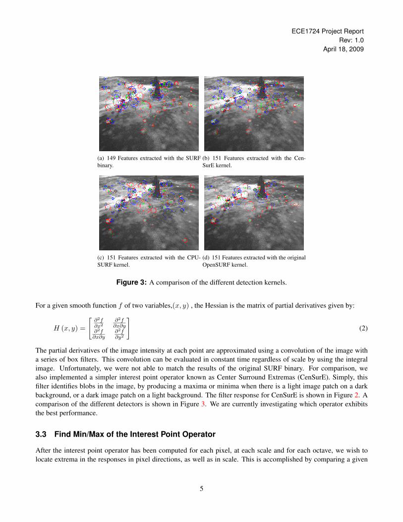
(a) 149 Features extracted with the SURFbinary.

(b) 151 Features extracted with the Cen-SurE kernel.

(c) 151 Features extracted with the CPU-SURF kernel.

(d) 151 Features extracted with the originalOpenSURF kernel.

Figure 3: A comparison of the different detection kernels.

For a given smooth function f of two variables,(x, y) , the Hessian is the matrix of partial derivatives given by:

H (x, y) =

[∂2f∂x2

∂2f∂x∂y

∂2f∂x∂y

∂2f∂y2

](2)

The partial derivatives of the image intensity at each point are approximated using a convolution of the image witha series of box filters. This convolution can be evaluated in constant time regardless of scale by using the integralimage. Unfortunately, we were not able to match the results of the original SURF binary. For comparison, wealso implemented a simpler interest point operator known as Center Surround Extremas (CenSurE). Simply, thisfilter identifies blobs in the image, by producing a maxima or minima when there is a light image patch on a darkbackground, or a dark image patch on a light background. The filter response for CenSurE is shown in Figure 2. Acomparison of the different detectors is shown in Figure 3. We are currently investigating which operator exhibitsthe best performance.

3.3 Find Min/Max of the Interest Point Operator

After the interest point operator has been computed for each pixel, at each scale and for each octave, we wish tolocate extrema in the responses in pixel directions, as well as in scale. This is accomplished by comparing a given

5


April 18, 2009

(a) The sample mask for finding maximum/minimumvalues Image credit: Lowe [5]

1 2 3 4 5 6 7 8 9 101112131415161718192021222324252627282930

123456789

1011121314

Block 1

Block 2

Block 3

Block 4

(b) A 2D slice of interest point data loaded onto shared memory

Figure 4

pixel value to its 8 neighbors in the given scale and the 9 neighbors in each of the scales above and below. Thisprocedure amounts to finding values that are greater than/less than its 26 neighbors arranged in a 3× 3× 3 cube asshown in Figure 4(a).

The basic flow of the algorithm on the GPU is as follows:

• Each block loads a 16× 8× 4 (x-y-scale) section of interest point operator into shared memory.

• A border of 1 in each dimension is used.

• Extrema calculation is computed for a centered 14× 6× 2 sub-block of loaded data.

• Data block loads must be overlapped due to border effects.

• If an extrema is found add to extrema array using an atomic increment to get a unique index.

A sketch of the overlapping image blocks is shown in Figure 4(b). The bold outlines show which elements eachblock operates on.

3.4 Find Sub-Pixel/Sub-Scale Interest Point

After all the response extrema have been located, a sub-pixel (and scale) interpolation is performed to further im-prove the localization of the interest point. The step is called as a separate kernel with a linear set of blocks eachcorresponding to an extremum.

Equation 3 shows a second order Taylor series expansion of the interest point operator function denoted as L.This defines a parabola fixed by the value and the first and second derivatives of L.

L(x + ∆x) = L(x) +(∂L

∂x

)T∆x +

12

∆xT(∂2L

∂x2

)∆x (3)

6


April 18, 2009

6s

6s

(a) Lattice Points

−1

−1

1

1

4s

(b) Haar filters

Fig. 4. The setup used to calculate feature orientation. (a) The lattice pointswhere Haar responses are sampled. (b) The Haar filters used to estimate localorientation. The gray dot is the lattice point about which the filter is sampled.

that high texture cache pressure evicts the block containing thefirst pixel before the adjacent ones are referenced. In contrast,the R-C texture is computed on a regular grid, making efficientuse of the texture cache. Measurements confirm that the two-lookup approach requires 33% less time than the three-lookupapproach, greatly outweighing the extra cost of computing theR-C texture for moderate feature counts. With this approach,evaluating arbitrarily-sized sub-pixel Haar responses in boththe x and y directions requires just 16 lookups.

D. Orientation Detection

The Haar responses used to find the dominant orientation ofa feature are sampled at the 113 lattice points inside a circle ofradius 6, scaled and offset by the feature scale and location, asillustrated in Fig. 4. The results are stored in a single texturerow corresponding to that feature. We tested two methods ofgenerating the lattice point locations from the target renderinglocation in the row. The first uses a simple mapping from the1D column index into a 2D square, followed by Early Z tomask out the points that lie outside the circle. The secondconverts the points inside the circle into a series of scan lineswhere each point has the same y coordinate and then rendersone quadrilateral per scan line, using texture coordinates tospecify the x coordinates. This latter method tested to be over20% faster than using Early Z. Another alternative we did nottest is simply using a 1D lookup texture.

Given the Haar response vectors, the CPU algorithm sortsthem by angle and uses a sliding window to extract the domi-nant orientation. Sorting on the GPU is notoriously slow, witheven the best parallel algorithms still comparable to a goodserial algorithm on the CPU [15]. Instead we approximate thesort using a 256-bin histogram. This is constructed with theRender to Vertex Buffer (R2VB) scattering algorithm proposedin [16]. Instead of accumulating a count of the vectors that fallin each bin, we accumulate the vectors themselves using alphablending, so there is no loss in angular resolution. The 7 Series

5s

5s

5s

5s

20s

θ

(a) Lattice Points

1−1

2s

−1

1

− cos(θ)− sin(θ)

cos(θ)− sin(θ)

− cos(θ)+ sin(θ)

cos(θ)+ sin(θ)

sin(θ)− cos(θ)

− sin(θ)− cos(θ)

sin(θ)+ cos(θ)

− sin(θ)+ cos(θ)

(b) Haar filters

Fig. 5. The setup used to calculate a feature vector. (a) The lattice pointswhere Haar responses are sampled. (b) The Haar filters used to compute thefeature vector values. The responses from the two axis-aligned filters at thetop are rotated to effectively achieve the pair of filters at the bottom.

GPUs cannot perform alpha blending on 32-bit floating pointtextures, so this step is limited to 16 bits of precision.

Once the vectors are assigned to histogram bins, we com-pute a cumulative histogram using Blelloch’s parallel prefixsum algorithm from Section III-A.2. Additionally, since allof these vectors have only two components, we can packthe values from two rows into a single texel and use theGPU’s four-wide vector operators to process both rows at once.Armed with this cumulative histogram, we can now computethe sum over the sliding window with just two or threelookups. Another up-sweep-like reduction is used to find thevector sum with the maximum magnitude, and its orientationis assigned to the corresponding feature. The approximationsmade in this approach do not impair the accuracy, yielding anRMS error of 0.20 degrees compared to the CPU algorithm.

E. Feature Vector Calculation

To construct the feature vectors, axis-aligned Haar responsesare computed on a 20s× 20s grid, as illustrated in Figure 5.The lattice points of the grid are aligned with the featureorientation, and the Haar response vector is rotated by thisangle as well. Each row of the output texture is used to storea single feature vector, with every texel value containing thefour elements of v. Normalization is done on the GPU usinganother simple reduction to compute the vector magnitude.

IV. RESULTS

We ran our implementation on a GeForce Go 7950 GTX anda GeForce 8800 GTX using images provided by Mikolajczyk4

as well as several downscaled versions of the frac.pgmimage included with SiftGPU [4]. Fig. 6 plots the average

4http://www.robots.ox.ac.uk/%7Evgg/research/affine/

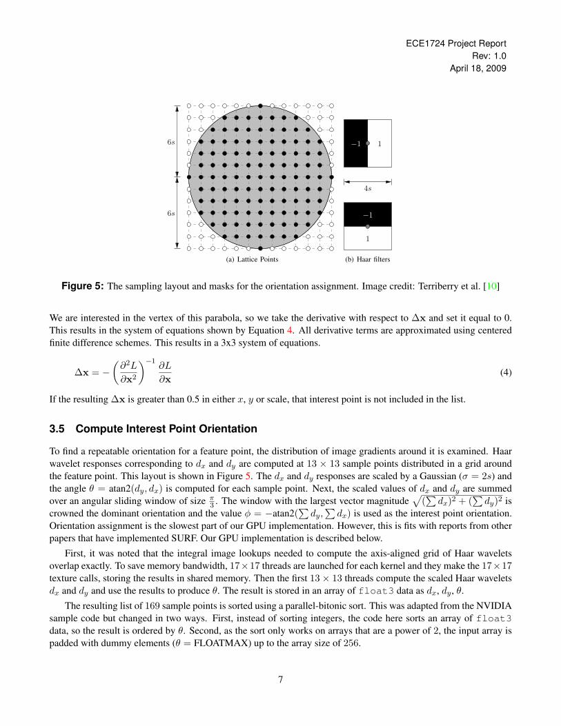
Figure 5: The sampling layout and masks for the orientation assignment. Image credit: Terriberry et al. [10]

We are interested in the vertex of this parabola, so we take the derivative with respect to ∆x and set it equal to 0.This results in the system of equations shown by Equation 4. All derivative terms are approximated using centeredfinite difference schemes. This results in a 3x3 system of equations.

∆x = −(∂2L

∂x2

)−1∂L

∂x(4)

If the resulting ∆x is greater than 0.5 in either x, y or scale, that interest point is not included in the list.

3.5 Compute Interest Point Orientation

To find a repeatable orientation for a feature point, the distribution of image gradients around it is examined. Haarwavelet responses corresponding to dx and dy are computed at 13 × 13 sample points distributed in a grid aroundthe feature point. This layout is shown in Figure 5. The dx and dy responses are scaled by a Gaussian (σ = 2s) andthe angle θ = atan2(dy, dx) is computed for each sample point. Next, the scaled values of dx and dy are summedover an angular sliding window of size π

3 . The window with the largest vector magnitude√

(∑dx)2 + (

∑dy)2 is

crowned the dominant orientation and the value φ = −atan2(∑dy,∑dx) is used as the interest point orientation.

Orientation assignment is the slowest part of our GPU implementation. However, this is fits with reports from otherpapers that have implemented SURF. Our GPU implementation is described below.

First, it was noted that the integral image lookups needed to compute the axis-aligned grid of Haar waveletsoverlap exactly. To save memory bandwidth, 17×17 threads are launched for each kernel and they make the 17×17texture calls, storing the results in shared memory. Then the first 13× 13 threads compute the scaled Haar waveletsdx and dy and use the results to produce θ. The result is stored in an array of float3 data as dx, dy, θ.

The resulting list of 169 sample points is sorted using a parallel-bitonic sort. This was adapted from the NVIDIAsample code but changed in two ways. First, instead of sorting integers, the code here sorts an array of float3data, so the result is ordered by θ. Second, as the sort only works on arrays that are a power of 2, the input array ispadded with dummy elements (θ = FLOATMAX) up to the array size of 256.

7


April 18, 2009

Finally, each of the 169 threads selects an angle in the sorted list and marches along the sorted array summingup all dx and dy values in the π

3 window. This is followed by a simple reduction to find the largest squared vectorlength (

∑dx)2 + (

∑dy)2. Again, the array is padded with dummy values so that the reduction can work on 256

elements.

As stated before, this ends up being the slowest part of our GPU algorithm. Several different optimizationmethods have been tried including:

1. Reducing the amount of shared memory used.

2. Replacing the sort with a linear search.

3. Calculating the final angle after the reduction to avoid 169 calls to atan2(·)

For whatever reason, each of these optimizations makes the kernel slower.

3.6 Compute Interest Point Descriptor

To construct the interest point descriptors, first, a square region of 20s× 20s centered around the interest point andoriented along the orientation computed in the previous section is defined. The region is then split up equally intosmaller 4×4 square subregions. For each sub-region, Haar wavelet responses are computed at 5×5 regularly spacedsample points. The lattice of sample points is illustrated in Figure 6. While the wavelet responses, dx and dy aredefined to be aligned to the primary orientation, it is more efficient to compute the axis-aligned responses, and rotatethem accordingly. Each of the responses are weighted by a Gaussian (σ = 3.3s), centered at the interest point.

The wavelet responses and their absolute values are then summed up over each sub-region, forming a four-entry descriptor vector for each sub-region (v = (

∑dx,∑dy,∑ |dx| ,

∑ |dy|)). Concatenating this for all 4 × 4sub-regions results in a descriptor vector of length 64. Finally, the descriptor vector is normalized into a unit vector.

For the GPU implementation, we decided to use two kernels: one to compute the unnormalized descriptors, anda second to conduct the normalization step. This substantially simplifies the code, since thread indexing is clearerwithout the need for bit masking. Initially, this was implemented as a single kernel, but too much shared memory wasused per block. Upon profiling, it was observed that cubin allocated local memory for this kernel when compiledfor our laptop, which prompted the split. Using the desktop computers, this split made the kernel marginally slower(likely due to the extra global memory read and write).

The first kernel call allocates 16 blocks per interest point (reflecting the 4 × 4 subregions), and 25 threads perblock (5× 5 sample points per subregion). The algorithm then progresses as follows:

1. Load interest point parameters (x, y, s, φ) into shared memory.

2. Compute trigonometric rotations (sin (φ) , cos (φ)).

3. Compute sample point locations.

4. Load integral image lookups (9 per sample point).

5. Compute axis-aligned Haar filter responses (dx, dy).

6. Rotate and store the Haar filter responses in shared memory.

8


April 18, 2009

6s

6s

(a) Lattice Points

−1

−1

1

1

4s

(b) Haar filters

Fig. 4. The setup used to calculate feature orientation. (a) The lattice pointswhere Haar responses are sampled. (b) The Haar filters used to estimate localorientation. The gray dot is the lattice point about which the filter is sampled.

that high texture cache pressure evicts the block containing thefirst pixel before the adjacent ones are referenced. In contrast,the R-C texture is computed on a regular grid, making efficientuse of the texture cache. Measurements confirm that the two-lookup approach requires 33% less time than the three-lookupapproach, greatly outweighing the extra cost of computing theR-C texture for moderate feature counts. With this approach,evaluating arbitrarily-sized sub-pixel Haar responses in boththe x and y directions requires just 16 lookups.

D. Orientation Detection

The Haar responses used to find the dominant orientation ofa feature are sampled at the 113 lattice points inside a circle ofradius 6, scaled and offset by the feature scale and location, asillustrated in Fig. 4. The results are stored in a single texturerow corresponding to that feature. We tested two methods ofgenerating the lattice point locations from the target renderinglocation in the row. The first uses a simple mapping from the1D column index into a 2D square, followed by Early Z tomask out the points that lie outside the circle. The secondconverts the points inside the circle into a series of scan lineswhere each point has the same y coordinate and then rendersone quadrilateral per scan line, using texture coordinates tospecify the x coordinates. This latter method tested to be over20% faster than using Early Z. Another alternative we did nottest is simply using a 1D lookup texture.

Given the Haar response vectors, the CPU algorithm sortsthem by angle and uses a sliding window to extract the domi-nant orientation. Sorting on the GPU is notoriously slow, witheven the best parallel algorithms still comparable to a goodserial algorithm on the CPU [15]. Instead we approximate thesort using a 256-bin histogram. This is constructed with theRender to Vertex Buffer (R2VB) scattering algorithm proposedin [16]. Instead of accumulating a count of the vectors that fallin each bin, we accumulate the vectors themselves using alphablending, so there is no loss in angular resolution. The 7 Series

5s

5s

5s

5s

20s

θ

(a) Lattice Points

1−1

2s

−1

1

− cos(θ)− sin(θ)

cos(θ)− sin(θ)

− cos(θ)+ sin(θ)

cos(θ)+ sin(θ)

sin(θ)− cos(θ)

− sin(θ)− cos(θ)

sin(θ)+ cos(θ)

− sin(θ)+ cos(θ)

(b) Haar filters

Fig. 5. The setup used to calculate a feature vector. (a) The lattice pointswhere Haar responses are sampled. (b) The Haar filters used to compute thefeature vector values. The responses from the two axis-aligned filters at thetop are rotated to effectively achieve the pair of filters at the bottom.

GPUs cannot perform alpha blending on 32-bit floating pointtextures, so this step is limited to 16 bits of precision.

Once the vectors are assigned to histogram bins, we com-pute a cumulative histogram using Blelloch’s parallel prefixsum algorithm from Section III-A.2. Additionally, since allof these vectors have only two components, we can packthe values from two rows into a single texel and use theGPU’s four-wide vector operators to process both rows at once.Armed with this cumulative histogram, we can now computethe sum over the sliding window with just two or threelookups. Another up-sweep-like reduction is used to find thevector sum with the maximum magnitude, and its orientationis assigned to the corresponding feature. The approximationsmade in this approach do not impair the accuracy, yielding anRMS error of 0.20 degrees compared to the CPU algorithm.

E. Feature Vector Calculation

To construct the feature vectors, axis-aligned Haar responsesare computed on a 20s× 20s grid, as illustrated in Figure 5.The lattice points of the grid are aligned with the featureorientation, and the Haar response vector is rotated by thisangle as well. Each row of the output texture is used to storea single feature vector, with every texel value containing thefour elements of v. Normalization is done on the GPU usinganother simple reduction to compute the vector magnitude.

IV. RESULTS

We ran our implementation on a GeForce Go 7950 GTX anda GeForce 8800 GTX using images provided by Mikolajczyk4

as well as several downscaled versions of the frac.pgmimage included with SiftGPU [4]. Fig. 6 plots the average

4http://www.robots.ox.ac.uk/%7Evgg/research/affine/

Figure 6: The setup used to calculate a feature vector. (a) The lattice points where Haar responses are sampled. (b)The Haar filters used to compute the feature vector values. The responses from the two axis-aligned filters at the topare rotated to effectively achieve the pair of filters at the bottom. Image credit: Terriberry et al. [10]

7. Load and store absolute values |dx| into another shared memory block.

8. Sum the dx, |dx| responses (reduction).

9. Write back the unnormalized responses to global memory.

10. Repeat for dy, |dy|.

For this algorithm, since the sample points are aligned to the rotated axis, the integral image texture lookups do notline up, like in the orientation computation. However, there are some savings in that lookups are reused betweenthe dx and dy filters. Since memory read coalescing for textures is not well documented, spatial locality of memoryaccesses were attempted, but not confirmed. Additionally, in the reduction steps, 25 numbers needed to be summed.Though the standard approach is to extend the shared memory block to the next highest power of two (32), inthe interest of shared memory requirements, a reduction step was first taken using 9 threads to reduce from 25 to16 numbers. Then, conventional unrolled reduction was used. Some indexing tricks were used to overcome therestriction that grids can only be 2D, while this kernel configuration makes more sense as a 3D grid.

For the second kernel, 1 block was allocated per interest point, with 64 threads per block (corresponding to thedimensionality of the descriptor vectors). The algorithm is as follows:

1. Load the values of the descriptor into local registers.

2. Square the values and store them into shared memory.

3. Sum (reduce) the squared values.

9


April 18, 2009

Figure 7: A sample stereo pair of images from our test set.

4. Compute the square root of the sum (length of the vector).

5. Divide each of the descriptor values by the length and write back to global memory.

This algorithm is fairly straightforward, and easily coalesces the memory reads and writes. Bank conflicts areavoided, since each thread only accesses one memory location each.

4 Methodology and Evaluation

As we mentioned in Section 2.2, our basic methodology was as follows:

1. Verify that the OpenSURF implementation matches the description in the original paper [6] and, where possi-ble, matches the results from the original SURF binary.

2. Implement the GPU equivalent code.

3. Verify that the GPU equivalent code produces the same results.

For evaluation, we used a series of stereo test images of various sizes collected at the University of TorontoInstitute for Aerospace Studies. A sample stereo pair is shown in Figure 7. We used a sequence of eight stereo pairsat resolutions of 512×384, 640×480, 1024×768, and 1280×960. This section will detail the method and metricswe used to evaluate each step of the algorithm and the associated results.

4.1 Timing Summary

Here we present the summary of the timing performance for each of the algorithm’s subcomponents. Table 1 showsthe percentage of computation time spent on the feature point independent tasks in the upper half and the featurepoint dependant tasks in the lower half. We see for the first three tasks, their computational cost is split relativelyevenly, with slightly more time spent on the find min/max operations for the larger image sizes. For the feature pointdependant operations, by far the most time consuming step is the determination of the orientation of the featurepoint.

Figure 8 graphically shows the time requires to process the 20 test images. The first thing we notice, it a verynearly linear speed up with image size. Secondly, there is not one particular kernel operation that consumes vastly

10


April 18, 2009

Image Size 512x384 640x480 1024x768 1280x960Integral Image 35.1% 29.9% 27.3% 28.2%

Interest Point Operator 28.4% 31.0% 32.1% 31.9%Find Min/Max 36.5% 39.1% 40.6% 39.9%

Sub pixel-scale Interpolation 11.4% 10.9% 10.2% 9.9%Orientation 64.9% 64.7% 64.4% 65.0%Descriptor 23.7% 24.4% 25.5% 25.1%

Table 1: Percentage of time for computations feature point independent calculations [top] and dependant [bottom]

more time than the others. This simply indicates a balanced approached must be taken when optimization speedupsare considered.

0 200000 400000 600000 800000 1000000 1200000 1400000

0

50

100

150

200

250

300

350

GPU SURF Timings

Subpixel-Scale Interpolation Interest Point Operator Descriptor Integral ImageFind Min/Max Orientation Total

# of Pixels

Tim

e (m

s)

Figure 8: Computation time required to process all images of varying sizes

4.2 Overall Speedup

In addition to timing the individual parts of the algorithm, the processing time for complete runs were also profiled.Using a single test image over the four image sizes, the average processing time of 1000 trials for the GPU-SURFimplementation was compared against average times over 10 trials for the CPU implementations (OpenSURF andCPU-SURF). The timings do not include memory initializations, but do include memory transfers to and fromthe GPU. SURF was not profiled for these trials since without source code, the memory initializations could notbe isolated and excluded from the timing. Table 2 shows the results of the experiments on the SF2202 desktopcomputers.

As can be seen, CPU-SURF takes about 4x as long as the unmodified OpenSURF, which corresponds to the

11


April 18, 2009

Image Size 512x384 640x480 1024x768 1280x960Feature Count 957 1509 3032 3218CPU-SURF 961.86ms 1461.65ms 3409.69ms 4153.78msOpenSURF 251.27ms 384.95ms 998.29ms 1276.63msGPU-SURF 6.75ms 10.83ms 21.10ms 28.00ms

CPU-SURF Percent Speedup 14250% 13496% 16160% 14835%OpenSURF Percent Speedup 3722% 3554% 4731% 4559%

Table 2: Overall speedup comparison between the CPU and GPU implementations.

4x increase in time complexity due to the implementation of bilinear filtering. All and all, these numbers showa substantial speedup vs. the CPU-based algorithms. These numbers can be improved upon with asynchronousmemory transfers to and from the GPU.

4.3 Compute Integral Image

(a) Input test image. (b) CPU implementation. (c) GPU implementation.

Figure 9: Plots of rounding errors between float and integer (exact) representation of the integral image (lightervalue indicates more error).

As mentioned in Section 3.1, we wished to utilize the sub-pixel texture indexing capabilities of the GPU. How-ever, to use this feature, the texture must be composed of floats. As a result, the intensity values of the input imagewere converted from integers ([0, 255]) to normalized floats ((0, 1)). This results in a loss of precision, which is no-ticeable when compounded through addition, as in the case of the integral image. To gauge the error, we comparedthe integral images generated by the CPU and the GPU to an exact integral image computed from the integer values.Figure 9 shows a sample image, and plots of the errors for our CPU and GPU implementations. Computing the RMSerrors, the CPU had a value of 0.0397, whereas the GPU had a value of 0.0066. While the GPU implementationhas a much lower error, we have not been able to explain this. We suspect that a combination of low precision androunding resulted in a series of fortunate errors.

To compare the following parts of the algorithm, we needed to ensure the inputs were the same. Since the GPUobtained more correct results, we decided to use the GPU’s results, by copying the computed integral image back tohost memory. However, we discovered that although the same integral image is used, sub-pixel lookups still remain

12


April 18, 2009

slightly different. Appendix D.2 of the CUDA Programming Guide details the algorithm for how bilinear filteringis done, but the actual hardware implementation details are not revealed. Therefore, we could not reverse-engineerand emulate the results produced by the GPU on the CPU, so the algorithms past this point will not produce exactlythe same results. However, it is expected that the results are very similar in the majority of cases. For some series ofcomputations, the values may be unstable, due to the lack of denormals on the GPU (which then order of operationsmatter). However, robustness is still present due to the large number of feature points identified by the algorithm,and these spurious features would simply not be used. One possible hint to the cause of the difference in texturelookup values is that the Appendix mentions that the fractional part is stored in 9-bit fixed point format, with 8 bitsof fractional value.

4.4 Compute Interest Point Operator

−1 −0.8 −0.6 −0.4 −0.2 0 0.2 0.4 0.6 0.8 1

x 10−3

0

1

2

3

4

5

6

7

8

9

10x 10

7

difference

coun

t

Differences between the CPU and GPU interest operator matrices.

Figure 10: A histogram of difference between the CPU and GPU implementations of the interest point operatorover all images.

Figure 10 shows the error difference between the interest operator computed on the CPU and GPU over all testimages. Once again, we believe the errors that are observed are due to the inexact texture lookups on the GPU.

4.5 Find Min/Max of the Interest Point Operator

When the CPU and GPU operate on identical interest point operator data, the CPU and GPU implementation de-termined the same extrema points. For the complete GPU implementation, slight discrepancies resulting from thetexture lookups in the interest point calculation resulted in a set of features which was very similar, but not identical.

4.6 Find Sub-Pixel/Sub-Scale Interest Point

Again, for verification purposes, we ensure the CPU and GPU versions are operating on the same interest point datato ensure we are only verifying the algorithm’s accuracy. As we see from figure 11 the majority of the errors are lessthan 0.2× 10−6 which is approaching on the machine precision accuracy of the float data type.

13


April 18, 2009

−1 −0.8 −0.6 −0.4 −0.2 0 0.2 0.4 0.6 0.8 1

x 10−6

0

2

4

6

8

10

12x 10

4

Interpolation error

coun

t

Histogram of interpolation error

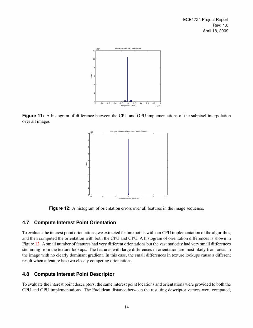
Figure 11: A histogram of difference between the CPU and GPU implementations of the subpixel interpolationover all images

−3 −2 −1 0 1 2 30

1

2

3

4

5

6

7

8

9x 10

4

orientation error (radians)

coun

t

Histogram of orientation error on 88055 features

Figure 12: A histogram of orientation errors over all features in the image sequence.

4.7 Compute Interest Point Orientation

To evaluate the interest point orientations, we extracted feature points with our CPU implementation of the algorithm,and then computed the orientation with both the CPU and GPU. A histogram of orientation differences is shown inFigure 12. A small number of features had very different orientations but the vast majority had very small differencesstemming from the texture lookups. The features with large differences in orientation are most likely from areas inthe image with no clearly dominant gradient. In this case, the small differences in texture lookups cause a differentresult when a feature has two closely competing orientations.

4.8 Compute Interest Point Descriptor

To evaluate the interest point descriptors, the same interest point locations and orientations were provided to both theCPU and GPU implementations. The Euclidean distance between the resulting descriptor vectors were computed,

14


April 18, 2009

0 0.02 0.04 0.06 0.08 0.1 0.12 0.14 0.16 0.18 0.20

0.2

0.4

0.6

0.8

1

1.2

1.4

1.6

1.8

2x 10

4

descriptor error (Euclidean distance)

coun

t

Histogram of descriptor error on 88055 features

Figure 13: A histogram of descriptor error Euclidean distances over all features in the image sequence.

which can be seen as a histogram in Figure 13. Much like the previous sections, the algorithms do not match exactly,as expected. However, two points to note are the relatively small maximum error of 0.2, as well as that the largestpeak is the one next to zero. This is again, as expected, as the integral image lookups between the CPU and the GPUare slightly different. These results match that of the orientation error histogram - the only reason it is more spreadout is because the histogram bins in this case are smaller.

4.9 Visual Odometry

As we stated in the introduction, our interest in this algorithm is it’s use in mobile robot navigation. To this end,the current code has been integrated into code that processes stereo images, tracks features through the images andproduces an estimate of the camera’s motion. We ran the algorithm using both SURF and GPU-SURF. The resultsare shown in Figure 14. All settings passed to the algorithm were the same, the only difference was the featuredetection/description algorithm. This is not a rigorous evaluation of one algorithm against another, it is simply ademonstration that our GPU-SURF implementation can be used for tracking features through image sequences. TheGPU code was called synchronously and GPU computations were not overlapped with CPU computations. Still,this resulted in a general speedup. The images used were 512 × 384 and the SURF algorithm ran at 3.7 Hz, whilethe GPU-SURF algorithm ran at 9.1 Hz.

5 Conclusions

We have successfully implemented a version of the SURF feature detector on the GPU. Where possible, we haveverified that our implementation matches the original paper and validated our results against a parallel CPU imple-mentation. Over the next few weeks, we will be integrating the algorithm into a real-time robot navigation system.This will involve the following steps:

15


April 18, 2009

0 20 40 60 80 1000

10

20

30

40

50

60

70

80

90

X (m)

Y (

m)

Truth GPU−SURF SURF

(a) Top-down view of the robot’s path

0 100 200 300 400 500 600 700 800 900−4

−2

0

2

X (

m)

Time (s)

0 100 200 300 400 500 600 700 800 900−4

−2

0

2

Y (

m)

Time (s)

0 100 200 300 400 500 600 700 800 900−15

−10

−5

0

Z (

m)

Time (s)

0 100 200 300 400 500 600 700 800 9000

1020

Euc

lidea

n er

ror

(m)

Time (s)

GPU−SURF SURF

(b) Translational error

0 100 200 300 400 500 600 700 800 900−10

−5

0

5

X (

deg)

Frame

0 100 200 300 400 500 600 700 800 900−6

−4

−2

0

2

Y (

deg)

Time (s)

0 100 200 300 400 500 600 700 800 900−10

−5

0

5

Z (

deg)

Frame

GPU−SURF SURF

(c) Rotational error

Figure 14: Comparison of SURF and GPU-SURF on a short visual odometry dataset.

16


April 18, 2009

1. Refactoring of the code to embed it in a C++ framework for autonomous robot navigation.

2. Implementation of feature matching to find matches between features in stereo images.

3. Use of CUDA streams to overlap image transfer and GPU computation.

4. Asynchronous execution of CPU and GPU code.

Once the code is integrated into this framework, we can perform the evaluation to determine the performance of ouralgorithm compared to other feature tracking schemes.

References

[1] David Nister and Henrik Stewenius. Scalable recognition with a vocabulary tree. In CVPR ’06: Proceedings ofthe 2006 IEEE Computer Society Conference on Computer Vision and Pattern Recognition, pages 2161–2168,Washington, DC, USA, 2006. IEEE Computer Society.

[2] T. D. Barfoot. Online visual motion estimation using FastSLAM with SIFT features. In Intelligent Robots andSystems, 2005. (IROS 2005). 2005 IEEE/RSJ International Conference on, pages 579–585, 2005.

[3] M. Brown and D.G. Lowe. Recognising panoramas. Computer Vision, 2003. Proceedings. Ninth IEEE Inter-national Conference on, pages 1218–1225 vol.2, Oct. 2003.

[4] Stephen Se and Piotr Jasiobedzki. Stereo-vision based 3d modeling and localization for unmanned vehicles.International Journal of Intelligent Control and Systems, 13(1):47–58, March 2008. Special Issue on FieldRobotics and Intelligent Systems.

[5] D. G. Lowe. Distinctive image features from scale-invariant keypoints. International Journal of ComputerVision, 60(2):91–110, 2004.

[6] Herbert Bay, Andreas Ess, Tinne Tuytelaars, and Luc Van Gool. Speeded-Up Robust Features (SURF). Com-put. Vis. Image Underst., 110(3):346–359, 2008.

[7] David Nister, Oleg Naroditsky, and James Bergen. Visual odometry for ground vehicle applications. Journalof Field Robotics, 23(1):3, 2006.

[8] Kurt Konolige, Motilal Agrawal, and Joan Sola. Large scale visual odometry for rough terrain. In Proceedingsof the International Symposium on Research in Robotics (ISRR), November 2007.

[9] N. Cornelis and L. Van Gool. Fast scale invariant feature detection and matching on programmable graphicshardware. pages 1–8, June 2008.

[10] Timothy B. Terriberry, Lindley M. French, and John Helmsen. GPU accelerating speeded-up robust features.In Proceedings of the 4th International Symposium on 3D Data Processing, Visualization and Transmission(3DPVT’08), pages 355—362, Atlanta, Georgia, June 2008.

[11] Motilal Agrawal, Kurt Konolige, and Morten Blas. Censure: Center surround extremas for realtime featuredetection and matching. In Computer Vision ECCV 2008, volume 5305/2008 of Lecture Notes in ComputerScience, pages 102–115. Springer Berlin / Heidelberg, 2008.

17


April 18, 2009

[12] Changchang Wu. SiftGPU: A GPU implementation of scale invariant feature transform (SIFT). http://cs.unc.edu/˜ccwu/siftgpu, 2007.

[13] Marten Bj orkman. A CUDA implementation of SIFT. http://www.csc.kth.se/˜celle/, 2009.

[14] Chris Evans. Open source SURF feature extraction library. http://code.google.com/p/opensurf1/, 2009.

18

http://cs.unc.edu/~ccwu/siftgpu

http://cs.unc.edu/~ccwu/siftgpu

http://www.csc.kth.se/~celle/

http://code.google.com/p/opensurf1/

http://code.google.com/p/opensurf1/

ECE1724 Project Report: ECE1724 ProjectSpeeded-Up Speeded...

Documents

Transcript of ECE1724 Project Report: ECE1724 ProjectSpeeded-Up Speeded...