Instabilities and speeded-up flavor equilibration in neutrino clouds

Ray Sawyer

UCSB

Domain of Application: Neutrino clouds with # densities of about (7 MeV)3 (but with non-thermal distributions) just under “neutrino-surface” in SN.

Phenomena: 1. Rapid exchange of flavors 2. Consequent hardening of e spectrum ……softening of spectra.

Mechanics:

Instabilities in (mean-field) non-linear evolution equations.

Bonus: Beyond the mean-field……..

comparison of stable and unstable cases

Overview

Time scales:

Very fast:

Medium fast:Kostelecki & Samuel 1995Raffelt , Sigl 2007Esteban-Pretel et al 2007G Fuller group RFS 2004 2005Hannestad et al 2006 (“bimodal”)

Oscillation:

Time scales:

Very fast:

Medium fast:

Oscillation:

this talk

Faster flavor scrambling of spectra —in a disorganized medium.

Also: relatively independent ofelectron neutrino excess, and normal vs. Inverted hierarchy

This term doesn’t contribute anything.

Density operators:

Forward Hamiltonian:

Commutation rules:

Angle dependence is key

Interactions:

Sum is over states, p, q that are occupied by ’s of some flavor.

Equations of motion:

oscillation term

Mean field approximation:

Take flavor diagonal initial conditions (two flavors):

and solve

Pastor and Raffelt (2002)

Momentum distribution xe near -sphere

We can delete e when paired in angle.

So, in effect,

Two beams------N up , N down (and no osc. terms)

For the up-moving states define,

For the down-moving states similarly,

Collective coordinates

Hamiltonian

E of M

Initials:

=1 neutrinos

=0 photons

With these initial conditions (and in mean field): Nothing happens. But when =0 there is an instability for rapid growth of a perturbation.

Eigenvalues of linearized problem:

Growth

So - in the photon problem we would get mixing time scale,

if no matter how tiny

In problem =1, ., marginally stable.

Including flavor-diagonal parts of mass terms (inverted hierarchy) get =complex.

and “medium fast”

(Kotkin & Serbo)

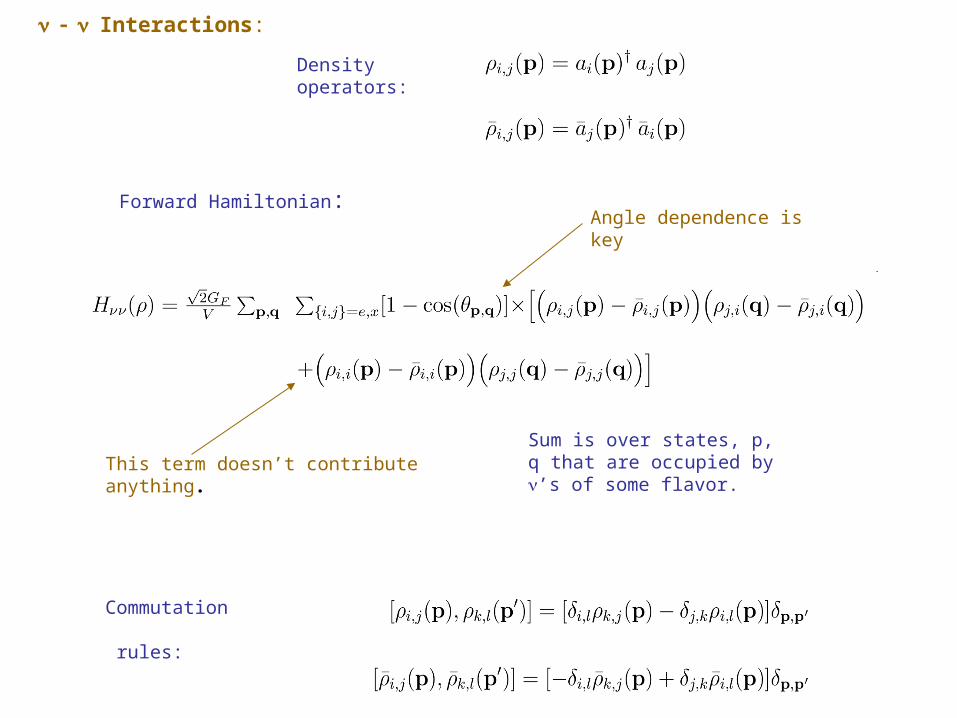
Back to

Now do 14 beam casebut in 3-space , & interpolating the up-down asymmetry of 2-beam simulation

Linearized stability analysis-- taking only the flavor-diagonal part of

A. Inverted hierarchy: Get a complex eigenvalue quite generally.

B. Normal hierarchy:

Get a complex eigenvalue only in the case of very small e excess.

In complete simulations of the evolution –with all of :

This complex e.v . complete scrambling of the angles and energies on the medium-fast time scale

This mixing rate and restriction on excess is roughly in accord with

results

of Raffelt and Sigl (suitably scaled to their region above surface)

But wait:

A. Take our initial assignments of densities in the various rays —

B. Introduce random variations of order 10% in these assignments

Then-- 60% of the time there is a complex ev even when

(no mass term at all)

In these cases, complete simulation gives total scrambling

for both normal and inverted hierarchies

Normal hierarchy

Inverted hierarchy

Results of solving 56 coupled nonlinear equations over 1000’s of oscillation times.

We have found that complete mixing ensues whenever the 28x28 matrix for the linear response has a complex eigenvalue.

Fourteen beams

Units (n GF)-1

50 = .5 cm

Upper hemispheree-x dens. Diff.

Implications for supernova

There will be rapid spectral mixing just under the surface, given the chaotic flows produced by SN simulations

The most interesting question is:

If in SN simulations the spectra are artificially scrambled at each time step,

……. would it affect the gross features of the hydrodynamics ??

A. If no: we may be done –

except for the possible application to R process nucleosynthesis

B. If yes, there is more to do.--

Take some data from a simulation with detailed angular distributions. Fit to a bunch of rays, and test the eigenvalues of the linearized system .

and the neutrino pulse from SN 2047h.

Beyond the mean field (in two beam case)

With no oscillation term or no Initial tilt------- the MF equations say that nothing happens.

But we can estimate in PT a flavor mixing time

Or, we can just solve the system

Case A: 1 --- stable (neutrinos)

(again)

Case B: 0 ---- unstable (photons)

Friedland & Lunardini (2003)

Friedland , McKellar, Okuniewicz (2006)

In a box of vol.= V

N=# of ’s

n =N/V

Conjecture: General connection between complex ev. in MF result and

log N behavior in complete solution..

under the influence of

Spin system: How long for this:

to go into this?

or this?

time in units (GN)-1

N=512

N=8

Comments: A logarithm is never large.

Coherence lengths?

Conclusion

Irregularities in flow

Instability in mean field linearized eqns.

Rapid flavor scrambling Interesting beyond-mean-field results ??

Should do beyond MF including mass terms

We defined MF approximation by taking operators, O:

taking commutators , [ H,O] , to get E of M ,

and then <>’s to get MF eqns.

Now, instead, take the operators

commute with H and take <>’s , getting closed set of 6 eqns.

Scaling time and density:

N=8192

N=8

Steps= factors of 4

Solid curves --- solutions to

Dashed curves --- solutions

Photon-photon scat:

(polarizations now take the place of flavors and Heisenberg-Euler replaces Z-exchange.)

laser

Laser: 2.35 eV,

100 MeV

Both beams linearly polarized.

Angle between polarizations not = n

Mean distance for scattering of the photon –from cross-section and laser beam density -- 109 cm.

Question: What is distance for polarization exchange?

Answer: 3 cm. (Kotkin and Serbo)

laserphoton cloud

Now with one cloud unpolarized and the other polarized:The polarized cloud loses polarization in distance 3 log[N] cm.

RFS Phys.Rev.Lett. 93 (2004) 133601

Colliding photon clouds