Hybrid-Trefftz finite elementmethod for heat conductionin nonlinear functionally

graded materialsZhuo-Jia Fu

Department of Engineering Mechanics, Hohai University,Nanjing, People’s Republic of China

Qing-Hua QinSchool of Engineering, Australian National University,

Canberra, Australia, and

Wen ChenDepartment of Engineering Mechanics, Hohai University,

Nanjing, People’s Republic of China

Abstract

Purpose – The purpose of this paper is to develop a hybrid-Trefftz (HT) finite element model (FEM)for simulating heat conduction in nonlinear functionally graded materials (FGMs) which caneffectively handle continuously varying properties within an element.

Design/methodology/approach – In the proposed model, a T-complete set of homogeneoussolutions is first derived and used to represent the intra-element temperature fields. As a result, thegraded properties of the FGMs are naturally reflected by using the newly developed Trefftz functions(T-complete functions in some literature) to model the intra-element fields. The derivation of theTrefftz functions is carried out by means of the well-known Kirchhoff transformation in conjunctionwith various variable transformations.

Findings – The study shows that, in contrast to the conventional FEM, the HT-FEM is an accuratenumerical scheme for FGMs in terms of the number of unknowns and is insensitive to mesh distortion.The method also performs very well in terms of numerical accuracy and can converge to the analyticalsolution when the number of elements is increased.

Originality/value – The value of this paper is twofold: a T-complete set of homogeneous solutionsfor nonlinear FMGs has been derived and used to represent the intra-element temperature; and thecorresponding variational functional and the associated algorithm has been constructed.

Keywords Finite element analysis, Heat conduction, Materials management

Paper type Research paper

The current issue and full text archive of this journal is available at

www.emeraldinsight.com/0264-4401.htm

The authors would like to thank Leilei Cao for her early assistance in computer programming.The work described in this paper was supported by the National Basic Research Program ofChina (973 Project No. 2010CB832702) and opening fund of State Key Lab of Structural Analysisof Industrial Equipment (GZ0902). The first author would also like to thank the ChinaScholarship Council (CSC) and Fundamental Research Funds for the Central Universities (GrantNo. 2010B15214) for financial support.

EC28,5

578

Received 8 July 2010Revised 15 October 2010Accepted 21 October 2010

Engineering Computations:International Journal forComputer-Aided Engineering andSoftwareVol. 28 No. 5, 2011pp. 578-599q Emerald Group Publishing Limited0264-4401DOI 10.1108/02644401111141028

1. IntroductionFunctionally graded materials (FGMs) are a new generation of composite materialswhose microstructure varies from one material to another with a specific gradient.In particular:

[. . .] a smooth transition region between a pure ceramic and pure metal would result in amaterial that combines the desirable high-temperature properties and thermal resistance of aceramic, with the fracture toughness of a metal (Gray et al., 2003).

By virtue of their excellent behaviours, FGMs have become increasingly popular inmaterials engineering and have featured in a wide range of engineering applications(e.g. thermal barrier materials (Erdogan, 1995), optical materials (Koike, 1991),electronic materials (Tani and Liu, 1993) and biomaterials (Pompe et al., 2003)).

During the past decades, extensive studies have been carried out on developingnumerical methods for analyzing thermal behaviours of FGMs (Kim and Paulino, 2002;Sutradhar and Paulino, 2004; Wang and Qin, 2008; Wang et al., 2006). For example, FEM(Kim and Paulino, 2002), the boundary element method (Sutradhar and Paulino, 2004) andthe meshless method (Wang and Qin, 2008; Wang et al., 2006) have been widely used toanalyze the thermal responses of FGMs. In contrast to the three methods above,hybrid-Trefftz (HT)-FEM (Qin, 2005) seems to be more suitable for numerical simulation ofFGMs, as Trefftz functions, which can reflect naturally the graded material properties, areused as internal interpolation for approximating elemental fields. It should be mentionedthat HT-FEM, introduced in 1977 (Jirousek and Leon, 1977), is a class of FE associatedwith the Trefftz method (Kamiya and Kita, 1995; Li et al., 2007). Trefftz method is apowerful numerical scheme for the solution of boundary value problem (Cheung et al.,1989; Van Genechten et al., 2010). It chooses Trefftz functions as basis function, which arealso called as T-complete functions or T-complete set of regular homogeneous solutions inliterature. The mathematical fundamentals of T-complete sets are established mainly byHerrera and his co-workers (Herrera and Sabina, 1978; Herrera, 1980). Since it combinesadvantages of the FEM and Trefftz method, the HT-FEM has now become a highlyefficient and well-established computational tool and been successfully applied to variousengineering problems, such as, e.g. plane elasticity (Dhanasekar et al., 2006), Kirchhoffplates (Qin, 1994), thick plates (Petrolito, 1990; Qin, 1995), general three-dimensional solidmechanics (Peters et al., 1994), potential problems (Wang et al., 2007; Zielinski andZienkiewicz, 1985), Helmholtz problems (Sze and Liu, 2010), transient heat conductionanalysis (Jirousek and Qin, 1996), and piezoelectric materials (Qin, 2003a, b) and contactproblems (Qin and Wang, 2008; Wang et al., 2005). Unlike the conventional FEM, HT-FEMis based on a hybrid method which includes imposing intra-element continuity to link upthe nonconforming internal fields with the inter-element frame field (Qin, 2000). Suchintra-element fields are chosen as suitable T-complete functions so as to a priori satisfy thegoverning equation of the problem under consideration. As indicated by Qin (2000), themain advantages of this method are:

. it only needs numerical integration along the element boundaries, which enablesarbitrary polygonal or even curve-sided shapes to be generated;

. it has high accuracy and a fast convergence rate ( Jirousek et al., 1993); and

. it permits great liberty in element geometry and provides the possibility ofaccurate performance without requiring annoying mesh adjustment to variouslocal effects thanks to loading and/or geometry (Dhanasekar et al., 2006).

Hybrid-TrefftzFEM for heat

conduction

579

Considering that the conventional FEM is inefficient for handling materials whosephysical property varies continuously, this paper presents a new element model whoseintra-element interpolation functions, called T-complete functions, can reflect varyingproperties. A brief outline of the paper is as follows: Section 2 presents a set ofnewly derived T-complete functions by means of the Kirchhoff transformation. Thecorresponding variational functional and Trefftz finite element formulation aredescribed in Section 3. In Section 4, three typical examples are considered to demonstratethe numerical efficiency and accuracy of the proposed HT-FEM. Finally, Section 5presents some conclusions and potential extensions of the proposed model.

2. Basic equation and their Trefftz functions2.1 Governing equations and their boundary conditionsConsider a two-dimensional (2D) heat conduction problem in an anisotropic nonlinearFGM, occupying a 2D arbitrary-shaped region V , R

2 bounded by its boundary G,and in the absence of heat sources. The governing differential equation is:X2

i;j¼1

›

›xi

Kijðx;TÞ›TðxÞ

›xj

� �¼ 0; x [ V ð1Þ

with the boundary conditions:

. Dirichlet/essential condition:

TðxÞ ¼ �T; x [ GD ð2aÞ

. Neumann/natural condition:

qðxÞ ¼ 2X2

i;j¼1

Kij›TðxÞ

›xj

niðxÞ ¼ �q; x [ GN ð2bÞ

where T is the temperature, G ¼ GD þ GN , ni is outward normal vector, and K ¼{Kijðx;TÞ}1#i;j#2 denotes the thermal conductivity matrix which satisfies thesymmetry K12 ¼ K21 and positive definite DK ¼ detðKÞ ¼ K11K22 2 K2

12 . 0. {ni} isthe outward unit normal vector at boundary x [ G.

2.2 Trefftz functionsTrefftz functions play an important role in the derivation of the HT-FE formulation(Qin, 2005). In this subsection, the construction of Trefftz functions for heat conductionin nonlinear FGMs is discussed in detail.

The nonlinear and anisotropic properties of equation (1) make it difficult to generatethe related Trefftz functions. To bypass this problem, the Kirchhoff transformationand mathematical variable transformation are used in the derivation. To this end, webegin with assuming that the coefficients of heat conduction are exponential functionsof the space coordinates as follows:

Kijðx;TÞ ¼ aðTÞ �KijeP2

i¼12bixi ; x ¼ ðx1; x2Þ [ V ð3Þ

EC28,5

580

in which a(T) . 0, �K ¼ { �Kij}1#i;j#2 is a symmetric positive-definite matrix, and thevalues are all real constants. b1 and b2 are two material constants.

By employing the Kirchhoff transformation:

fðTÞ ¼

ZaðTÞdT ð4Þ

Equations (1) and (2) can be reduced to the following form:

X2

i;j¼1

�Kij

›2FTðxÞ

›xi›xj

þX2

m¼1

X2

n¼1

2bm�Kmn

›FTðxÞ

›xn

!eP2

i¼12bixi ¼ 0; x [ V ð5Þ

FTðxÞ ¼ fð �TÞ; x [ GD ð6aÞ

qðxÞ ¼ 2X2

i;j¼1

Kij

›TðxÞ

›xj

niðxÞ ¼ 2eP2

i¼12bixi

X2

i;j¼1

�Kij

›FTðxÞ

›xj

niðxÞ ¼ �q; x [ GN ð6bÞ

where FT ðxÞ ¼ wðTðxÞÞ and the inverse Kirchhoff transformation yields:

TðxÞ ¼ w21ðFTðxÞÞ ð7Þ

The simplest way to find the Trefftz functions of equation (5) is by using the followingtwo transformations.

To simplify the expression of equations (5) and (6), set FT ¼ Ce2P2

i¼1bixi .

Then equations (5) and (6) can be rewritten as follows:

X2

i;j¼1

�Kij›CðxÞ

›xi›xj

2 l 2CðxÞ

!eP2

i¼1bixi ¼ 0; x [ V ð8Þ

C ¼ fð �TÞeP2

i¼1bixi ; x [ GD ð9aÞ

qðxÞ ¼ 2eP2

i¼1bixi

X2

i;j¼1

�Kij›C

›xj

2 bjC

� �niðxÞ ¼ �q; x [ GN ð9bÞ

in which:

l ¼

ffiffiffiffiffiffiffiffiffiffiffiffiffiffiffiffiffiffiffiffiffiffiffiffiffiffiffiffiffiffiX2

i¼1

X2

j¼1

bi�Kijbj

vuutSince e

P2

i¼1bixi . 0, hence the Trefftz functions of equation (8) are equal to those of

anisotropic modified Helmholtz equation.

Hybrid-TrefftzFEM for heat

conduction

581

To find the solution of equation (8), we set:

y1

y2

!¼

1=ffiffiffiffiffiffiffi�K11

p0

2 �K12=ffiffiffiffiffiffiffiffiffiffiffiffiffi�K11D �K

q ffiffiffiffiffiffiffi�K11

p=ffiffiffiffiffiffiD �K

p0B@

1CA x1

x2

!ð10Þ

where D �K ¼ detð �KÞ ¼ �K11�K22 2 �K

212 . 0.

It follows from equation (8) that:

X2

i¼1

›2Cð yÞ

›yi›yi

2 l 2Cð yÞ

!¼ 0; y [ V ð11Þ

Hence, we have the Trefftz solutions for equation (8) in the form:

I 0ðlrÞ; ImðlrÞcosðmuÞ; ImðlrÞsinðmuÞ m ¼ 1; 2; . . . ; ðr; uÞ [ V ð12Þ

where:

r ¼

ffiffiffiffiffiffiffiffiffiffiffiffiffiffiy2

1 þ y22

q; u ¼ arctan

y2

y1

� �

and Im denotes the m-order modified Bessel function of first kind.Therefore, the Trefftz functions of equation (5) can be represented as:

I 0ðlrÞe2P2

i¼1bixi ;

ImðlrÞcosðmuÞe2P2

i¼1bixi ;

ImðlrÞsinðmuÞe2P2

i¼1bixi m ¼ 1; 2; . . .

ð13Þ

3. HT-FE formulation3.1 Assumed fieldsTo perform HT-FE analysis, the whole domain V is divided into a number of elements.For a particular element, say element e, occupying a sub-domain Ve with the elementboundary Ge, two groups of independent fields are assumed in the following way(Qin, 2005):

. A non-conforming intra-element field is defined by:

ueðxÞ ¼Xm

j¼1

NejðxÞcej ¼ NeðxÞce ;x [ Ve ð14Þ

where ce stands for unknown parameters and m represents the number of homogeneoussolutions (Trefftz terms). Nej are the homogeneous solutions to equation (8):

EC28,5

582

Ne1 ¼ I 0ðlrÞ;

Ne2 ¼ ImðlrÞcos u;

Ne3 ¼ ImðlrÞsin u; . . . ;

Neð2mþ1Þ ¼ ImðlrÞsinðmuÞ; . . .

It should be mentioned that the assumed intra-element temperature field here is definedin a local reference system x ¼ (x1, x2) whose axis remains parallel to the axis of theglobal reference system X ¼ (X1, X2) (Figure 1(a)).

The corresponding outward normal derivative of ue on Ge is defined by:

qe ¼ 2X2

i;j¼1

Kij

›ue

›xj

ni ¼ Qece ð15Þ

where:

Qe ¼ 2X2

i;j¼1

Kij›Ne

›xj

niðxÞ ¼ 2AKTe ð16Þ

with:

A ¼ n1 n2

h i; Te ¼

›Ne

›x1

›Ne

›x2

" #T

ð17Þ

The undetermined coefficients c, here, may be calculated in many different ways(variational approach, least square, etc.) that enable the prescribed boundary conditionsand the inter-element continuity to be approximately fulfilled. The simplest way toenforce the inter-element continuity conditions:

ue ¼ uf on Ge > Gf conformity ð18aÞ

qe þ qf ¼ 0 on Ge > Gf reciprocity ð18bÞ

and to express the unknown coefficients c in terms of conveniently chosen nodalparameters is a hybrid procedure based on using a frame function representing an

Figure 1.(a) Intra-element field in a

particular element and(b) typical quadratic

interpolation for the framefield

X2

X2

X1

X1

Node Centroid

(a) (b)

1

1 – x2

2

2

2

–

3

N2

N1

N3

x = –1 x = 0 x = +1

x (1– x)

x (1+ x)

Hybrid-TrefftzFEM for heat

conduction

583

independent temperature u. So, the second independent temperature field should beintroduced in the following way:

. An auxiliary exactly and minimally conforming frame field:

~ueðxÞ ¼ ~NeðxÞde; x [ Ge ð19Þ

is independently assumed along the element boundary Ge in terms of nodal degrees offreedom (DOF) de, where Ne represents the conventional finite element interpolatingfunctions. For instance, a quadratic interpolation of the frame field on any side withthree nodes of a particular element (Figure 1(b)) can be given in the form:

~u ¼ ~N1u1 þ ~N2u2 þ ~N3u3 ð20Þ

where Ni (i ¼ 1, 2, 3) denotes shape functions in terms of natural coordinate j shown inFigure 1(b).

3.2 Modified variational principle and stiffness equationThe HT-FE formulation for heat conduction in nonlinear FGMs can be established bythe variational approach (Qin, 2005; Wang and Qin, 2009). The approach is basedmainly on a modified variational principle. The terminology “modified principle” refershere to the use of conventional potential functional and some modified terms for theconstruction of a special variational principle. The reason for using the modifiedterms is that satisfaction of continuity temperature and heat flow between elements(equation (18)) and heat flow boundary conditions cannot be guaranteed in theHT-FEM due to the use of Trefftz functions as the shape function within an element.Following the procedure given by Wang and Qin (2009), the functional correspondingto the problem defined in equations (8) and (9) is constructed as:

Pm ¼e

XPme ð21Þ

with:

Pme ¼ 21

2

ZVe

e2P2

i¼1bixi U; iU ;i

� �dV2

ZGqe

�q~udGþ

ZGe

qð~u 2 uÞdG

þ

ZGe

e2P2

i¼1bixi

X2

i;j¼1

�KijbjniU2

!dG

ð22Þ

in which:

U ;1 ¼ffiffiffiffiffiffiffi�K11

p ›U

›x1þ

�K12ffiffiffiffiffiffiffi�K11

p ›U

›x2; U ;2 ¼

ffiffiffiffiffiffiD �K

pffiffiffiffiffiffiffi�K11

p ›U

›x2with U ¼ ue

P2

i¼1bixi :

It should be mentioned that in functional (22), the governing equation (8) is satisfied,a priori, due to the use of Trefftz solutions in the HT-FE model. The boundary Ge of aparticular element consists of the following parts:

EC28,5

584

Ge ¼ Gue < Gqe < GIe and Gue > Gqe ¼ Gqe > GIe ¼ Gue > GIe ¼ B ð23Þ

where GIe represents the intra-element boundary of the element “e”.Next, we prove that the stationary condition of the functional (21) leads to the

governing equation (5), boundary conditions (6) and continuity conditions (18). Thefirst-order variational of the functional (22) yields:

dPme ¼ 2

ZVe

EeP2

i¼1bixi dVþ

ZGe

FeP2

i¼1bixi dG2

ZGqe

�qd~udG

þ

ZGe

dqð~u 2 uÞdGþ

ZGe

qðd~u 2 duÞdG

ð24Þ

where:

E ¼X2

i;j¼1

�Kiju;j þ �Kijbj

� �du;i þ l 2u þ �Kijbju;i

� �du

� �ð25Þ

F ¼X2

i;j¼1

2 �Kijbjniudu ð26Þ

By using the divergence theorem:ZV

f ;ih;j þ h72f� �

dV ¼

ZG

hf ;injdG ð27Þ

where f and h are two arbitrary functions in the solution domain, functional (24) can bewritten as:

dPme ¼

ZVe

eP2

i¼1bixiX2

i;j¼1

�Kijðu;ij 2 l2uÞ

!dV2

ZGqe

ð�q 2 qÞd~udG

þ

ZGe

dqð~u 2 uÞdGþ

ZGIe

qd~udGþ

ZGue

qd~udG

ð28Þ

For the temperature-based method, the potential conformity is satisfied in advance,that is:

d~u ¼ d�u ¼ 0 on Gueðu ¼ ~uÞ d~ue ¼ d~uf on GIef ð~ue ¼ ~uf Þ ð29Þ

Then, equation (28) can be rewritten as:

dPme ¼

ZVe

eP2

i¼1bixi

X2

i;j¼1

�Kijðu;ij 2 l2uÞ

!dV2

ZGqe

ð�q 2 qÞd~udG

þ

ZGe

dqð~u 2 uÞdGþ

ZGIe

qd~udG

ð30Þ

from which the governing equation (8) and boundary conditions (9) can be obtainedusing the stationary condition dPme ¼ 0:

Hybrid-TrefftzFEM for heat

conduction

585

X2

i;j¼1

�Kij

›2uðxÞ

›xi›xj

2 l 2uðxÞ

!eP2

i¼1bixi ¼ 0; x [ V ð31Þ

u ¼ fð �TÞeP2

i¼1bixi ; x [ GD ð32aÞ

qðxÞ ¼ 2eP2

i¼1bixi

X2

i;j¼1

�Kij›u

›xj

2 bju

� �niðxÞ ¼ �q; x [ GN ð32bÞ

We can produce the field continuity requirement equation (18) in the following way.When assembling elements “e” and “f”, we have:

dPmðeþf Þ ¼

ZVeþf

eP2

i¼1bixi

X2

i;j¼1

�Kijðu;ij 2 l 2uÞ

!dV2

ZGqeþqf

ð�q 2 qÞd~udG

þ

ZGe

dqð~u 2 uÞdGþ

ZGf

dqð~u 2 uÞdGþ

ZGIef

qd~uef dGþ · · ·

ð33Þ

From which the vanishing variation of dPmðeþf Þ leads to the reciprocity condition (18b)qe þ qf ¼ 0 on the intra-element boundary GIef.

Therefore, the functional (22) can be used to generate the element stiffness equationused in this work through the variational approach described in Qin (2000). Applyingthe divergence theorem again to the functional (22), we have the final functional for theHT-FE model:

Pme ¼ 21

2

ZGe

qudG2

ZGqe

�q~udGþ

ZGe

q~udG ð34Þ

Substituting equations (14), (15) and (19) into the functional (34) yields:

Pe ¼ 21

2cTeHece 2 dT

e ge þ cTe Gede ð35Þ

in which:

He ¼

ZGe

QTe NedG Ge ¼

ZGe

QTe~NedG ge ¼

ZGeq

~NT

e �qdG

To enforce inter-element continuity on the common element boundary, the unknownvector ce shoufld be represented in terms of the nodal DOF de. An optional relationshipbetween ce and de in the sense of variation can be obtained by minimization of thefunctional Pe with respect to ce:

›Pe

›cTe

¼ 2Hece þ Gede ¼ 0 ð36Þ

which leads to:

ce ¼ H21e Gede ð37Þ

EC28,5

586

and then yields the expression Pe only in terms of de and other known matrices:

Pe ¼1

2dT

e GTe H

21e Gede 2 dT

e ge ð38Þ

Therefore, by taking the vanishing functional Pe with respect to de:

›Pe

›dTe

¼ GTe H

21e Gede 2 ge ¼ 0 ð39Þ

the stiffness equation can be expressed as:

Kede 5 ge ð40Þ

where Ke 5GTe H

21e Ge stands for the element stiffness matrix.

It is worth noting that the evaluation of the right-hand vector ge in equation (40) isthe same as that in conventional FEM, which is obviously convenient for theimplementation of HT-FEM into existing FEM programs.

3.3 Recovery of constant temperature in the domainConsidering the physical definition of the Trefftz functions, it is necessary to recoverthe missing constant temperature modes in the domain from the above results.

Following the method presented by Qin (2000), the missing constant temperature inthe domain can be recovered by writing the internal potential field of a particularelement e as:

ue ¼ Nece þ c0 ð41Þ

where the undetermined constant temperature parameter c0 in the domain can becalculated using the least square matching of ue and ue at element nodes:

Xn

i¼1

ðNece þ c0 2 ~ueÞ2jnode i ¼ min ð42Þ

which finally gives:

c0 ¼1

n

Xn

i¼1

Duei ð43Þ

in which Duei ¼ ð~ue 2NeceÞjnode i and n is the number of element nodes.Once the nodal field is determined by solving the final stiffness equation, the

coefficient vector ce can be evaluated from equation (40), and then C0 is evaluated fromequation (43). Finally, the potential field u at any internal point in an element can beobtained by means of equation (41).

It should be pointed out that the potential field obtained by the proposed HT-FEM isthe solution of equations (8) and (9). Therefore, it needs to use two inversetransformations in obtaining the temperature field T:

(1) FT ¼ ue2P2

i¼1bixi .

(2) TðxÞ ¼ w21ðFTðxÞÞ.

Hybrid-TrefftzFEM for heat

conduction

587

4. Numerical assessments and discussionsIn this section, the efficiency, accuracy and convergence of the HT-FEM are tested byconsidering three heat conduction problems in FGMs. The results of the proposedmethod are compared with the MFS solution and analytical solution. To provide amore quantitative understanding of the results, the average relative error Rerr(w) andnormalised error Nerr(w) defined, respectively, by:

RerrðwÞ ¼

ffiffiffiffiffiffiffiffiffiffiffiffiffiffiffiffiffiffiffiffiffiffiffiffiffiffiffiffiffiffiffiffiffiffiffiffiffiffiffiffiffiffiffiffi1

NT

XNT

i¼1

wði Þ2 �wði Þ

�wði Þ

��������2

vuut ; ð44Þ

NerrðwÞ ¼jwði Þ2 �wði Þj

1#i#NTmax j �wði Þj

; ð45Þ

are employed in numerical analysis, where w(i ) and w(i ) are the analytical andnumerical solutions at xi, respectively, and NT denotes the total number of uniform testpoints in the domain of interest. Unless otherwise specified, NT is taken to be 100 andfive-point Gauss-Legendre quadrature rule is used for numerical integration in all thefollowing numerical analysis.

Example 1. First a 0.04 £ 0.04 square plate graded along the x1 direction isconsidered (Wang and Qin, 2009). The thermal conductivity K ¼ K0eb1x1 , whereK0 ¼ 1 and b1 ¼ 50, the corresponding value in equation (3) is:

aðTÞ ¼ 1; �K ¼1 0

0 1

!; b1 ¼ 1; b2 ¼ 0:

The analytical solution is:

TðxÞ ¼eb1x1 2 1

e 0:04b1 2 1ð46Þ

subject to the following boundary conditions:

qðxÞ ¼ 0; x1 ¼ 0; qðxÞ ¼ 0; x1 ¼ 0:04; TðxÞ ¼ 0; x2 ¼ 0; TðxÞ ¼ 1; x2 ¼ 0:04

Since the properties of the FGM are independent of temperature, there is no need to usethe Kirchhoff transformation in this example. Table I presents, respectively, the effectof the terms M of Trefftz functions on the average relative error Rerr, the conditionnumber of stiffness matrix K, and the Trefftz interpolation matrix H for element 1shown in Figure 2. Condition number Cond in Table I is defined as the ratio of thelargest singular value of matrix to the smallest. It can be observed from Table I that the

M 7 9 11 13

Rerr 1.204 £ 1022 7.346 £ 1023 7.371 £ 1023 1.185 £ 1022

Cond(K) 6.4043 6.4264 6.4236 6.4232Cond(H) 2.291 £ 108 2.730 £ 1011 5.424 £ 1014 8.743 £ 1015

Table I.Numerical results ofExample 1 with differentterms M of T-completefunctions in 2 £ 2 meshes

EC28,5

588

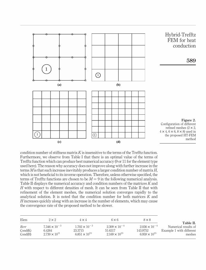
condition number of stiffness matrix K is insensitive to the terms of the Trefftz function.Furthermore, we observe from Table I that there is an optimal value of the terms ofTrefftz function which can produce best numerical accuracy (9 or 11 for the element typeused here). The reason why accuracy does not improve along with further increase in theterms M is that such increase inevitably produces a larger condition number of matrix H,which is not beneficial to its inverse operation. Therefore, unless otherwise specified, theterms of Trefftz functions are chosen to be M ¼ 9 in the following numerical analysis.Table II displays the numerical accuracy and condition numbers of the matrices K andH with respect to different densities of mesh. It can be seen from Table II that withrefinement of the element meshes, the numerical solution converges rapidly to theanalytical solution. It is noted that the condition number for both matrices K andH increases quickly along with an increase in the number of elements, which may causethe convergence rate of the proposed method to be slower.

Figure 2.Configuration of different

refined meshes (2 £ 2,4 £ 4, 6 £ 6, 8 £ 8) used in

the proposed HT-FEMmethod

1

(a) (b)

1

(d)

1

(c)

1

Elem 2 £ 2 4 £ 4 6 £ 6 8 £ 8

Rerr 7.346 £ 1023 1.702 £ 1023 2.309 £ 1024 2.036 £ 1024

Cond(K) 6.4264 23.3715 51.6317 143.9752Cond(H) 2.730 £ 1011 6.851 £ 1013 2.169 £ 1015 6.959 £ 1015

Table II.Numerical results of

Example 1 with differentmeshes

Hybrid-TrefftzFEM for heat

conduction

589

Example 2. Consider the heat transfer in a nonlinear FGM whose coefficients of heatconduction are defined by equation (3) with a(T) ¼ e T. This problem usually occurs inhigh-temperature environments. By using the Kirchhoff transformation, we can obtain:

FT ¼ eT ; T ¼ f21ðFTÞ ¼ lnðFTÞ:

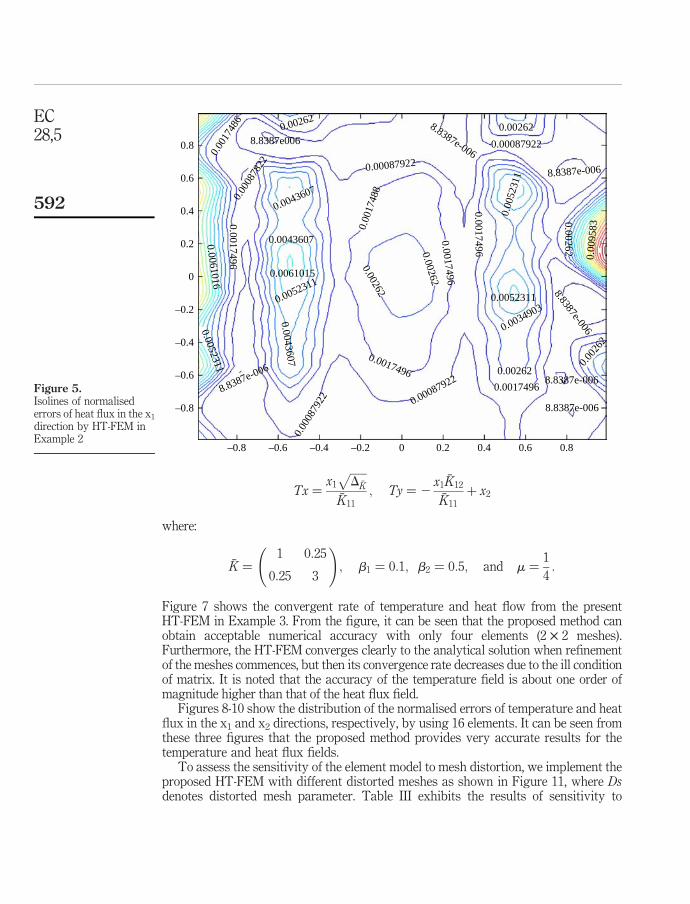
Let us consider an orthotropic material (Marin and Lesnic, 2007) in the squareV ¼ ð21; 1Þ £ ð21; 1Þ in which:

�K ¼2 0

0 1

!

and b1 ¼ 0;b2 ¼ 1. Its analytical solution is:

TðxÞ ¼ ln

ffiffiffiffiffiffiffiffiffiffiffiffiffiffiffiffiffiffiffiffiffiffi1 2 Tx=Tr

2Tr

rsinhðTrÞe2Ty

!ð47aÞ

FTðxÞ ¼ eTðxÞ ð47bÞ

where:

Tx ¼x1ffiffiffi

2p 2 1; Ty ¼ x2; Tr ¼

ffiffiffiffiffiffiffiffiffiffiffiffiffiffiffiffiffiffiffiffiffiffiTx 2 þ Ty 2

p:

Figure 3 shows the variations in the numerical accuracy of temperature and heat flux inx1 and x2 directions with mesh density. We can observe from Figure 3 that the resultsfrom the present HT-FEM agree well with the analytical solution and converge quicklyalong with the increasing number of elements. Figures 4-6 show the distribution ofnormalised errors of temperature and heat flux, respectively, by HT-FEM with 4 £ 4meshes. It can be observed that the results are again in good agreement with theanalytical solution.

Figure 3.Rerr of temperature andheat flux versus number ofelements in Example 2

0

10–1

10–2

10–3

10–410 20 30 40 50

Tqxqy

60 70

Number of elements

Rer

r

EC28,5

590

Example 3. We next consider another type of nonlinear exponential FGM with the samegeometry V ¼ ð21; 1Þ £ ð21; 1Þ as in Example 2. In practice, the dependence of thethermal conductivity on the temperature may be chosen as linear, i.e. a(T) ¼ 1 þ mT,where m is a material constant. By using the Kirchhoff transformation, we can obtain:

FT ¼ T þm

2T 2; T ¼ f21ðFTÞ ¼

21 þffiffiffiffiffiffiffiffiffiffiffiffiffiffiffiffiffiffiffiffiffi1 þ 2mFT

pm

:

The analytical solution in this example is:

TðxÞ ¼21 þ

ffiffiffiffiffiffiffiffiffiffiffiffiffiffiffiffiffiffiffiffiffiffiffiffiffiffi1 þ 2mFTðxÞ

pm

ð48aÞ

FT ðxÞ ¼ e ðlðTxþTyÞ=tÞ2P2

i¼1bixi ð48bÞ

in which:

t ¼

ffiffiffiffiffiffiffiffiffiffiffiffiffiffiffiffiffiffiffiffiffiffiffiffiffiffiffiffiffiffiffiffiffiffiffiffiffiffiffiffiffiffiffiffiffiffiffiffiffiffiffiffiffiffiffiffiffiffiffiffiffiffiffiffiffiffiffiffiffiffiffiffiffiffiffiffiffiffiffiffiffiffiffiffiffiffiffiffiffiffiffiffiffiffiffiffiffi�K11

ffiffiffiffiffiffiD �K

p2 �K12

�K11

!2

þ2 �K12

ffiffiffiffiffiffiD �K

p2 �K12

�K11

!þ �K22

vuut

Figure 4.Isolines of normalised

errors of temperature byHT-FEM in Example 2

0.8

4.4512e-007

4.4512e-007

4.4512e-007

0.6

0.4

0.2

0

–0.2

–0.4

–0.6

–0.8

–0.8

–0.6 –0.4 –0.2

0.00055603

0.00

3889

5

0.00

0556

03

0.00

1946

0.00055603

0.00083382

0.00083382

0.00055603

0.00055603

0.000278240.

0002

7824

0.00138944.4512e-0070.0011116

0.0011116

0.00027824

0.00027824

0.00027824

0.00027824

0 0.2 0.4 0.6 0.8

Hybrid-TrefftzFEM for heat

conduction

591

Tx ¼x1

ffiffiffiffiffiffiD �K

p�K11

; Ty ¼ 2x1

�K12

�K11

þ x2

where:

�K ¼1 0:25

0:25 3

!; b1 ¼ 0:1; b2 ¼ 0:5; and m ¼

1

4:

Figure 7 shows the convergent rate of temperature and heat flow from the presentHT-FEM in Example 3. From the figure, it can be seen that the proposed method canobtain acceptable numerical accuracy with only four elements (2 £ 2 meshes).Furthermore, the HT-FEM converges clearly to the analytical solution when refinementof the meshes commences, but then its convergence rate decreases due to the ill conditionof matrix. It is noted that the accuracy of the temperature field is about one order ofmagnitude higher than that of the heat flux field.

Figures 8-10 show the distribution of the normalised errors of temperature and heatflux in the x1 and x2 directions, respectively, by using 16 elements. It can be seen fromthese three figures that the proposed method provides very accurate results for thetemperature and heat flux fields.

To assess the sensitivity of the element model to mesh distortion, we implement theproposed HT-FEM with different distorted meshes as shown in Figure 11, where Dsdenotes distorted mesh parameter. Table III exhibits the results of sensitivity to

Figure 5.Isolines of normalisederrors of heat flux in the x1

direction by HT-FEM inExample 2

0.8 8.8387e006

0.0043607

0.0061015

0.0052311

0.0052311

8.8387e-006

0.00

0879

22 0.00087922

0.0034903

0.00

9583

0.00

5231

1

0.0017496

0.00262

0.00

262

0.00262

0.0052311

0.00087922

0.00262

8.8387e-006

8.8387e-006

8.8387e-006

8.8387e-006

0.0017496

0.0017496

0.0017496

0.002620.00262

0.0017496

0.0061016

0.0043607

0.00262

0.00

1748

60.

0008

7822

0.0043607

0.00087922

0.00

1748

8

8.8387e-006

0.6

0.4

0.2

0

–0.2

–0.4

–0.6

–0.8

–0.8

–0.6 –0.4 –0.2 0 0.2 0.4 0.6 0.8

EC28,5

592

mesh distortion. The numerical results reveal that the proposed method is remarkablyinsensitive to mesh distortion, a result which is superior to that from the traditionalFEM, allowing greater freedom in element geometry and giving the possibility ofaccurate performance without troublesome mesh adjustment.

Figure 6.Isolines of normalised

errors of heat flux in the x2

direction by HT-FEM inExample 2

0.8

0.6

0.4

0.2

0

–0.2

–0.4

–0.6

–0.8

–0.8

–0.6 –0.4

0.0015295

0.0015295

0.0015295

0.0058735

8.1466e-005

8.1466e-005

8.1466e-0050.01

0217

0.0015295

0.0015295

0.0044255

0.0029775

0.0029775

0.00

2977

5

0.00

2977

5

0.002

9775

0.00442550.0044255

0.0044255

0.0029775

0.00

2977

5

0.0029775

0.0029775

0.001

5295

0.0015295

0.00

1529

5

–0.2 0 0.2 0.4 0.6 0.8

Figure 7.Variations in numerical

accuracy of temperatureand heat flux with number

of elements by HT-FEM

10–1

10–2

10–3

10–4

10–50 10 20 30 40 50 60 70

Number of elements

Tqx

qy

Rer

r

Hybrid-TrefftzFEM for heat

conduction

593

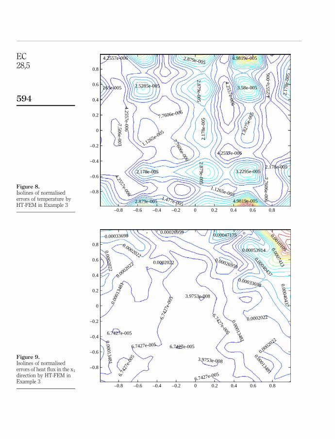
Figure 8.Isolines of normalisederrors of temperature byHT-FEM in Example 3

0.8

4.2557e-006

2.5285e-005

2.178e-0053.2295e-005

4.9819e-005

3.58e-005

2.17

8e-0

05

1.82

75e-

005

4.25

57e-

006

4.2557e-006

4.9819e-005

4.2557e-006

2.17

8e-0

05

2.178e-005

7.7606e-006

7.7606e-006

2.879e-005

2.879e-0052.879e-005

7.506e-007

4.2557e-006

2.879e-005

7.7606e-006

1.1265e-005

4.2557e-006

1.477e-005

1.1265e-005

265e-0050.6

0.4

0.2

0

–0.2

–0.4

–0.6

–0.8

–0.8

–0.6 –0.4 –0.2 0 0.2 0.4 0.6 0.8

Figure 9.Isolines of normalisederrors of heat flux in the x1

direction by HT-FEM inExample 3

0.8

0.6

0.4

0.2

0

–0.2

–0.4

–0.6

–0.8

6.7427e-005

6.7427e-005

6.74

27e-

005

6.7427e-005

3.9753e-008

3.9753e-008

0.00026959 0.00047175

0.00053914

0.0007413

0.000404370.0010109

0.000269590.0002022

0.0002022

0.0002022

0.00033698

0.00033698 0.00040437

0.0002022

0.0002022

0.0002022

6.74

27e-

005

6.7427e-005

0.00013481

0.00

0134

81

0.00013481

0.00013481

6.7427e-005

–0.8

–0.6 –0.4 –0.2 0 0.2 0.4 0.6 0.8

EC28,5

594

Figure 10.Isolines of normalised

errors of heat flux in the x2

direction by HT-FEM inExample 3

0.00023023

6968

9000

.0

5.0279e-0070.00023023

0.00023023

0.00023023

0.00023023

0.00068969

0.00

0160

86

0.000160860.00034464

0.00034464

0.00068969

0.00023023

0.00023023

0.00023023

0.00

0230

230.

0004

5996

5.02

79e-

007

5.0279e-007

5.02

79e-

007

5.0279e-007

0.00068969

0.00091942

0.000

1149

1

0.000114910.00011491

0.000

4599

6

0.00

0459

960.

0002

3023

0.00023023

0.00

0230

23

0.8

0.6

0.4

0.2

0

–0.2

–0.4

–0.6

–0.8

–0.8

–0.6 –0.4 –0.2 0 0.2 0.4 0.6 0.8

Figure 11.2 £ 2 distorted mesh for

Example 3Ds

1

Hybrid-TrefftzFEM for heat

conduction

595

Dis

tort

edp

aram

eter

Un

dis

tort

edD

s¼

0.3

Ds¼

0.4

Ds¼

0.6

Ds¼

0.7

Con

d(K

)3.

307

3.63

533.

3749

3.34

923.

6027

Con

d(H

)1.

778£

1010

8.43

1£

1010

4.06

6£

1010

7.32

6£

109

3.02

0£

109

Rer

rof

T2.

221£

102

45.

584£

102

45.

903£

102

43.

014£

102

45.

182£

102

4

Rer

rof

qx

4.47

7£

102

37.

698£

102

36.

349£

102

35.

700£

102

38.

239£

102

3

Rer

rof

qy

1.00

9£

102

21.

657£

102

21.

434£

102

21.

231£

102

21.

685£

102

2

Table III.Numerical results ofExample 3 with distortedand undistorted mesh(Ds ¼ 0.5)

EC28,5

596

5. ConclusionsIn this paper, we present a set of Trefftz functions for heat conduction problems inexponential FGMs by way of the Kirchhoff transformation and coordinate transformation.The Trefftz functions are then used for developing the HT-FE formulation for heatconduction analysis in 2D nonlinear FGMs. Numerical results demonstrate that theproposed HT-FEM is a competitive numerical method for the solution of heat conductionin nonlinear FGMs. The method performs very well in terms of numerical accuracy andcan converge to the analytical solution when the number of elements is increased. Theresults also demonstrate the insensitivity of the element model to mesh distortion. Futureextension of the proposed method can be made to cases of three-dimensional compositematerials (Berger et al., 2005) and transient heat transfer problems in FGMs (Kuo andChen, 2005; Sladek et al., 2005; Sutradhar et al., 2002). This work is under way.

References

Berger, J.R., Martin, P.A., Mantic, V. and Gray, L.J. (2005), “Fundamental solutions forsteady-state heat transfer in an exponentially graded anisotropic material”, Zeitschrift FurAngewandte Mathematik Und Physik, Vol. 56, pp. 293-303.

Cheung, Y.K., Jin, W.G. and Zienkiewicz, O.C. (1989), “Direct solution procedure for solution ofharmonic problems using complete, non-singular, Trefftz functions”, Comm. Appl. Num.Meth., Vol. 5, pp. 159-69.

Dhanasekar, M., Han, J.J. and Qin, Q.H. (2006), “A hybrid-Trefftz element containing an elliptichole”, Finite Elements in Analysis and Design, Vol. 42, pp. 1314-23.

Erdogan, F. (1995), “Fracture mechanics of functionally graded materials”, CompositesEngineering, Vol. 5, pp. 753-70.

Gray, L.J., Kaplan, T., Richardson, J.D. and Paulino, G.H. (2003), “Green’s functions and boundaryintegral analysis for exponentially graded materials: heat conduction”, Journal of AppliedMechanics-Transactions of the ASME, Vol. 70, pp. 543-9.

Herrera, I. (1980), “Boundary methods: a criterion for completeness”, Proc. Natl. Acad. Sci. USA,Vol. 77, pp. 4395-8.

Herrera, I. and Sabina, F.J. (1978), “Connectivity as an alternative to boundary integral equations:construction of bases”, Proc. Natl. Acad. Sci. USA, Vol. 75, pp. 2059-63.

Jirousek, J. and Leon, N. (1977), “A powerful finite element for plate bending”, Computer Methodsin Applied Mechanics and Engineering, Vol. 12, pp. 77-96.

Jirousek, J. and Qin, Q.H. (1996), “Application of hybrid-Trefftz element approach to transientheat conduction analysis”, Computers & Structures, Vol. 58, pp. 195-201.

Jirousek, J., Venkatesh, A., Zielinski, A.P. and Rabemanantsoa, H. (1993), “Comparative study ofp-extensions based on conventional assumed displacement and hybrid-Trefftz FEmodels”, Computers & Structures, Vol. 46, pp. 261-78.

Kamiya, N. and Kita, E. (1995), “Trefftz method 70 years”, Adv. Eng. Softw., Vol. 24 Nos 1-3.

Kim, J.-H. and Paulino, G.H. (2002), “Isoparametric graded finite elements for nonhomogeneousisotropic and orthotropic materials”, Journal of Applied Mechanics, Vol. 69, pp. 502-14.

Koike, Y. (1991), “High-bandwidth graded-index polymer optical fibre”, Polymer, Vol. 32,pp. 1737-45.

Kuo, H.Y. and Chen, T.Y. (2005), “Steady and transient Green’s functions for anisotropicconduction in an exponentially graded solid”, International Journal of Solids andStructures, Vol. 42, pp. 1111-28.

Hybrid-TrefftzFEM for heat

conduction

597

Li, Z.C., Tzon-Tzer, L., Hung-Tsai, H. and Cheng, A.H.D. (2007), “Trefftz, collocation, and otherboundary methods – a comparison”, Numerical Methods for Partial Differential Equations,Vol. 23, pp. 93-144.

Marin, L. and Lesnic, D. (2007), “The method of fundamental solutions for nonlinear functionallygraded materials”, International Journal of Solids and Structures, Vol. 44, pp. 6878-90.

Peters, K., Stein, E. and Wagner, W. (1994), “A new boundary-type finite element for 2-D- and3-D-elastic structures”, International Journal for Numerical Methods in Engineering,Vol. 37, pp. 1009-25.

Petrolito, J. (1990), “Hybrid-trefftz quadrilateral elements for thick plate analysis”, ComputerMethods in Applied Mechanics and Engineering, Vol. 78, pp. 331-51.

Pompe, W., Worch, H., Epple, M., Friess, W., Gelinsky, M., Greil, P., Hempel, U., Scharnweber, D.and Schulte, K. (2003), “Functionally graded materials for biomedical applications”,Materials Science and Engineering, Vol. A362, pp. 40-60.

Qin, Q.H. (1994), “Hybrid Trefftz finite-element approach for plate-bending on anelastic-foundation”, Applied Mathematical Modelling, Vol. 18, pp. 334-9.

Qin, Q.H. (1995), “Hybrid-Trefftz finite element method for Reissner plates on an elasticfoundation”, Computer Methods in Applied Mechanics and Engineering, Vol. 122,pp. 379-92.

Qin, Q.H. (2000), The Trefftz Finite and Boundary Element Method, WIT Press, Southampton.

Qin, Q.H. (2003a), “Solving anti-plane problems of piezoelectric materials by the Trefftz finiteelement approach”, Computational Mechanics, Vol. 31, pp. 461-8.

Qin, Q.H. (2003b), “Variational formulations for TFEM of piezoelectricity”, International Journalof Solids and Structures, Vol. 40, pp. 6335-46.

Qin, Q.H. (2005), “Trefftz finite element method and its applications”, Applied Mechanics Reviews,Vol. 58, pp. 316-37.

Qin, Q.H. and Wang, K.Y. (2008), “Application of hybrid-Trefftz finite element method tofrictional contact problems”, Computer Assisted Mechanics and Engineering Sciences,Vol. 15, pp. 319-36.

Sladek, V., Sladek, J., Tanaka, M. and Zhang, C. (2005), “Transient heat conduction in anisotropicand functionally graded media by local integral equations”, Engineering Analysis withBoundary Elements, Vol. 29, pp. 1047-65.

Sutradhar, A. and Paulino, G.H. (2004), “The simple boundary element method for transient heatconduction in functionally graded materials”, Computer Methods in Applied Mechanicsand Engineering, Vol. 193, pp. 4511-39.

Sutradhar, A., Paulino, G.H. and Gray, L.J. (2002), “Transient heat conduction in homogeneousand non-homogeneous materials by the Laplace transform Galerkin boundary elementmethod”, Engineering Analysis with Boundary Elements, Vol. 26, pp. 119-32.

Sze, K. and Liu, G. (2010), “Hybrid-Trefftz six-node triangular finite element models forHelmholtz problem”, Computational Mechanics, Vol. 46, pp. 455-70.

Tani, J. and Liu, G. (1993), SH Surface Waves in Functionally Gradient Piezoelectric Plates,Japan Society of Mechanical Engineers, Tokyo.

Van Genechten, B., Bergen, B., Vandepitte, D. and Desmet, W. (2010), “A Trefftz-based numericalmodelling framework for Helmholtz problems with complex multiple scattererconfigurations”, Journal of Computational Physics, Vol. 229 No. 18, pp. 6623-43.

Wang, H. and Qin, Q.H. (2008), “Meshless approach for thermo-mechanical analysis offunctionally graded materials”, Engineering Analysis with Boundary Elements, Vol. 32,pp. 704-12.

EC28,5

598

Wang, H. and Qin, Q.H. (2009), “Hybrid FEM with fundamental solutions as trial functions forheat conduction simulation”, Acta Mechanica Solida Sinica, Vol. 22, pp. 487-98.

Wang, H., Qin, Q.H. and Arounsavat, D. (2007), “Application of hybrid Trefftz finite elementmethod to non-linear problems of minimal surface”, International Journal for NumericalMethods in Engineering, Vol. 69, pp. 1262-77.

Wang, H., Qin, Q.H. and Kang, Y.L. (2006), “A meshless model for transient heat conduction infunctionally graded materials”, Computational Mechanics, Vol. 38, pp. 51-60.

Wang, K.Y., Qin, Q.H., Kang, Y.L., Wang, J.S. and Qu, C.Y. (2005), “A direct constrain-TrefftzFEM for analysing elastic contact problems”, International Journal for Numerical Methodsin Engineering, Vol. 63, pp. 1694-718.

Zielinski, A.P. and Zienkiewicz, O.C. (1985), “Generalized finite element analysis with T-completeboundary solution functions”, International Journal for Numerical Methods inEngineering, Vol. 21, pp. 509-28.

Corresponding authorQing-Hua Qin can be contacted at: qinghua.qin@anu.edu.au

Hybrid-TrefftzFEM for heat

conduction

599

To purchase reprints of this article please e-mail: reprints@emeraldinsight.comOr visit our web site for further details: www.emeraldinsight.com/reprints