Easy Structuring Max
68
Overview of Structured Products Maxime Poulin 2 Introduction A Structured product is a simple concept: it is a bond, which has a coupon and/or a redemption value which, rather than being fixed like a bond, is linked to an underlying price. A good example would be: a bond which does not pay any coupon throughout its life, but at maturity will be redeemed at its par value plus the best between zero and 100% of the performance of the underlying (an equity index for example) measured over the lifetime of the product. This very simple payoff can be split into two very simple financial instruments: A call option on the underlying and a zero coupon bond which will ensure the redemption at par (both instruments have the same notional amount). In this paper we will see what the manufacturing aspects of structured products are: from the pricing to the hedging as well as the distribution channel. We will try to cover the most commonly sold payoffs, their advantages on both sides: clients and sellers as well as the risks and costs they incur to the bank which issues them.
-
Upload
papalazorous -
Category
Documents
-
view
120 -
download
11
Transcript of Easy Structuring Max

Overview of Structured Products
Maxime Poulin 2
Introduction A Structured product is a simple concept: it is a bond, which has a coupon
and/or a redemption value which, rather than being fixed like a bond, is linked
to an underlying price.
A good example would be: a bond which does not pay any coupon throughout
its life, but at maturity will be redeemed at its par value plus the best between
zero and 100% of the performance of the underlying (an equity index for
example) measured over the lifetime of the product.
This very simple payoff can be split into two very simple financial instruments:
A call option on the underlying and a zero coupon bond which will ensure the
redemption at par (both instruments have the same notional amount).
In this paper we will see what the manufacturing aspects of structured
products are: from the pricing to the hedging as well as the distribution
channel. We will try to cover the most commonly sold payoffs, their
advantages on both sides: clients and sellers as well as the risks and costs
they incur to the bank which issues them.
Overview of Structured Products
Maxime Poulin 3
Index
Introduction....................................................................................................2
1. The Market Makers.................................................................................6
1.1. The Structure of the issuers (banks)..................................................6
1.2. The Profit and Loss Scheme .............................................................7
2. The Clients and the Intermediaries ......................................................9
3. Structured Products ............................................................................11
3.1. Definition..........................................................................................11
3.2. Building a Structured product ..........................................................11
3.3. Structured Products type .................................................................13
4. Derivatives used in Structured Products...........................................16
4.1. Vanilla Options ................................................................................16
4.2. Barrier Options ................................................................................18
4.3. Merging Options ..............................................................................20
5. Black-Scholes Model ...........................................................................22
5.1. Assumptions of the Black & Scholes model.....................................22
5.2. Stochastic Differential Equations (SDEs).........................................22
5.3. Lognormal returns for asset prices ..................................................23
5.4. The Black & Scholes formula...........................................................23
5.5. The Black & Scholes formulas for options .......................................23
5.6. Call – Put Parity...............................................................................24
6. The Forwards .......................................................................................26
7. The Correlation ....................................................................................27
7.1. Definition..........................................................................................27
7.2. Correlation term structure and skew................................................27
8. Volatility and Variance.........................................................................29
8.1. Definition..........................................................................................29
8.2. Implied Volatility...............................................................................29
8.3. Volatility term Structure....................................................................30

Overview of Structured Products
Maxime Poulin 4
8.4. Volatility Skew / Smile......................................................................30
9. Quanto and Compo Options ...............................................................33
10. Sensitivities of Exotic Options ...........................................................36
10.1. Time Value Relationship..................................................................36
10.2. Estimating sensitivities: Pragmatic approach...................................37
11. Models used on Trading floors (Commerzbank)...............................39
11.1. Calibration process of a model ........................................................40
11.2. How do Option pricing models operate?..........................................41
11.3. Black Vanilla Model .........................................................................46
11.4. Black Diffusion Model ......................................................................46
11.5. Local Volatility Model .......................................................................47
11.6. Stochastic Volatility Model ...............................................................47
11.6.1. The Heston Model.................................................................49
11.6.2. The Hagan Model .................................................................50
11.6.3. The Scott-Chesney Model ....................................................50
12. The risks related to structured products ...........................................51
12.1. Delta Risk ........................................................................................52
12.2. Vega Risk ........................................................................................52
12.3. Correlation Risk ...............................................................................53
12.4. Second order Risks .........................................................................53
13. Example of exotic derivative: Cliquets ..............................................55
13.1. Convexity (or Volga) ........................................................................55
13.2. Cliquets............................................................................................58
13.2.1. Classic Cliquet ......................................................................58
13.2.2. Ratchet Cliquet .....................................................................60
13.2.3. Reverse Cliquet ....................................................................62
13.2.4. Napoleon Cliquet ..................................................................65
Conclusion ...................................................................................................69
Bibliography.................................................................................................70
Overview of Structured Products
Maxime Poulin 5
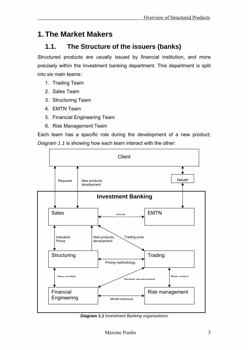
1. The Market Makers
1.1. The Structure of the issuers (banks) Structured products are usually issued by financial institution, and more
precisely within the Investment banking department. This department is split
into six main teams:
1. Trading Team
2. Sales Team
3. Structuring Team
4. EMTN Team
5. Financial Engineering Team
6. Risk Management Team
Each team has a specific role during the development of a new product;
Diagram 1.1 is showing how each team interact with the other:
Diagram 1.1 Investment Banking organizations
Pricing methodology
Model approval
Trading Structuring
Sales
Client
EMTN
Requests New products development
Indicative Prices
Trading price New products development
Issuer
Risk management
Risk control
Financial Engineering
New modelsModels development
Investment Banking
Issuer

Overview of Structured Products
Maxime Poulin 6
Each team (Trading, Sales, Structuring, etc) is also segmented into different
desks, depending on the asset class: Equity, Commodities, Fixed Income,
Currencies and Credit.
Trading will take care of the hedging and the pricing, while the sales team will
try to sell products at a fair price for the bank.
1.2. The Profit and Loss Scheme
As in every corporate group, the aim is to make profit, and mainly maximizing
those while taking as little risk as possible. Financial institutions like banks,
which offer financial products to their clients, have to bear some risk on these.
This risk taken on by the bank has to be hedged by the traders using tools
and techniques we will see further on.
But in this case, what is the value added for the bank, where does it make a
profit? In fact it works the same way than for most companies, the bank
determine a fair price for the financial product and sells it at a higher price.
This fair price is calculated using mathematical models which we will more in
detail in the “Pricing” section; represent the cost of fully hedging the product,
this assuming the pricing model is perfect.
If the Traders job is to hedge position taken by the bank when it sells financial
products, what explain the bonuses they receive each year? As we said
earlier the banks makes its profit by selling a financial product which has a
hedging cost of USD 98 at a higher price: USD 100 for example, incurring a
profit of USD 2 for the bank for each product sold with these characteristics.
But this assumes each product is fully hedged, although in facts, traders don’t
usually fully hedge their books. Meaning they keep some exposure to the
market in their books that they decide not to hedge. This is driven by the risk
aversion and the market views of each trader. By keeping a market exposure,
the traders increase the risk of their books which might lead to losses if the

Overview of Structured Products
Maxime Poulin 7
traders’ views were wrong, but on the other end might also lead to additional
earnings if they are right.
As a conclusion we can see that the total Profit and Loss of the bank will be
the sum of both the sales margin: selling at a higher price than the actual
hedging cost, and the traders profit or loss realised by not fully hedging his
position.
∑∑==
+=J
j
jTrader
I
i
iSalesLP
11PositionsMargin&
Where: “i” is the number of product sold and “j” the number of positions held
by the bank.
Overview of Structured Products
Maxime Poulin 8
2. The Clients and the Intermediaries
Structured products are sold to a wide range of clients: although very often
overpriced, structured products are very powerful tools in order to improve the
performance of a portfolio. Clients range from institutional investor to retail
investor, they are not interested in the same products: Institutional investor
usually only buy the option part of a structured product whereas retails
investor tend to go for bundles with both the option and the bond part.
The front office division (Sales Teams) cannot distribute directly these product
to all customers, moreover, it cannot tailor a product for a single retail investor
(size would be too small). On top of that the regulators do not allow them to
talk directly to retail customers due to their lack of awareness. The retail
market is maintained by companies such as: insurance companies, fund
management companies, brokers, banks (wealth management department),
financial advisors, family offices. Those companies have a very large
distribution network and an administration which allows them to speak directly
to the public.
These intermediaries are making profit by charging the client for their services
as well as receiving a commission from the product manufacturer. In this
case, the manufacturer will take this commission into account into its hedging
price.
Some intermediaries will only buy the option part of the structured product and
then manufacture the bond feature of the product themselves.
As a conclusion we can say that there are different types of product which will
be suitable for different investors:
• Fully manufactured products for small retail investors, brokers, or other
intermediary. This enables the product manufacturer to sell its product
to the general public without having to actually deal with them. These
customers / intermediaries are referred to as “Private Banks”: high
powered investors, asset managers, brokers who do not have the
capacity to manufacture structured products, but who are very lightly
regulated in regards to who they are marketing products to.

Overview of Structured Products
Maxime Poulin 9
• “Raw” Structured products: the option part of a structured product sold
to institutional investor. Very highly regulated and competitive
business.
There is a broad range of products available to each type of investors, but
most of them can be classified in to these three classes.
• Simple market access products
• Yield enhancement products
• Capital protected products
Overview of Structured Products
Maxime Poulin 10
3. Structured Products
3.1. Definition
A structured product can take the form of many different payoffs. But in
essence it is a bond (or certificate) which pays instead of the guaranteed
coupon offered by the bond, a payoff linked to the performance (either
positive or negative) of an underlying (which can be of any asset class:
commodity, equity, FX, interest rate).
A good example would be: a bond which does not pay any coupon throughout
its life, but at maturity will be redeemed at its par value plus a coupon of X% if
the performance of the underlying (an equity index for example) measured
over the lifetime of the product is positive.
This very simple payoff can be split into two very simple financial instruments:
A digitale option on the underlying and a zero coupon bond which will ensure
the redemption at par (both instruments have the same notional amount).
3.2. Building a Structured product
A structured product is composed of several pieces: the seller of such a
product will try to replicate each individual piece and sell them in a package.
In order to do so, the issuer will create the product through legal
documentation which will state exactly the terms and conditions of the
product: the exact obligation that the issuer has in regards to the investors.
The buyer will not in general have any physical proof of ownership of the
bond, but the exchange will go trough electronic settlement systems such as
Euroclear or Clearstream, and they will keep track of all these transactions.
Such structured products can take different legal form:
Overview of Structured Products
Maxime Poulin 11
• It can be issued as an investment fund: in this case, a fund is incorporated
and buys all parts of the structured product. The investor who bought
shares of this fund gain an identical exposure to the market than if he had
bought the pieces independently. This kind of legal form is mainly used for
regulation purpose. For example in the UK, the range products that can be
offered to the public are very restricted, but it is legal to sell investment
funds to the same public.
• The most common legal form is the Medium Term Note (MTN, and more
often in Europe: Euro MTN: EMTN). This is usually used by the issuer to
finance its business activities. For this legal form, the traders enter into a
swap with the bond issuer in which they will give an amount to the bond
issuer and receive a floating coupon generally equal to Libor plus or minus
Spread. This Spread is determined by the market’s required rate of return
to take the risk of that specific bond issuer.
• The second most common form is the certificate, there is not much
difference between the MTN (or EMTN) and the certificate. Regarding the
pricing: it has no impact on the pricing of the derivative, and the impact on
the bond part is only due to the funding given by the bond issuer.
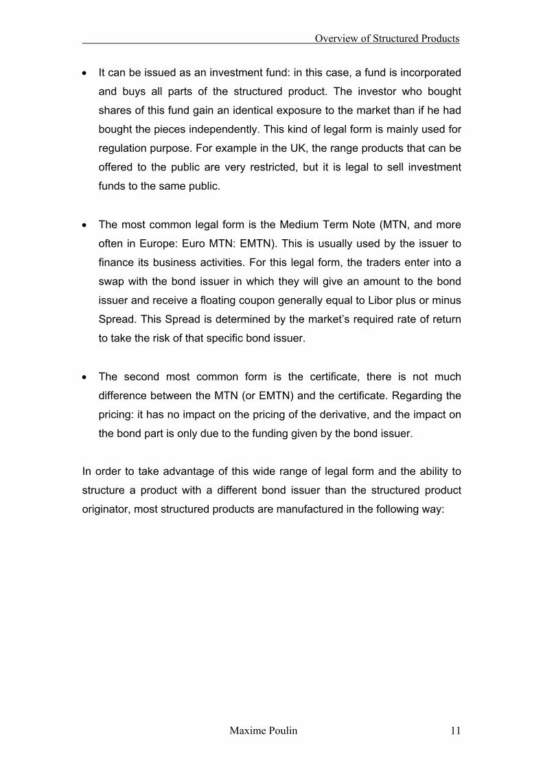
In order to take advantage of this wide range of legal form and the ability to
structure a product with a different bond issuer than the structured product
originator, most structured products are manufactured in the following way:
Overview of Structured Products
Maxime Poulin 12
Issuer, derivatives seller
Bond Issuer
Bond investor
Issuers pays Equity-linked amount to Bond issuer at maturity / Over bond lifetime
Bond issuer pays the Issuer:Coupon stream in format of Issuers choice (frequency,Currency etc.)
Bond investor pays bond issuer100 EUR for the bond atInception
Bond issuer sells bondWith desired equity-Linked payoff to bondinvestor
Diagram 3.1: Manufacture of Structured Products
In most cases the issuer and the bond issuer will be the same company, but
in some cases as per the investor request, the bond issuer will be a different
company than the structured product issuer. This can be due to two main
reasons: either the preference to trade with a better rated issuer (to reduce
the default risk), or receive a better funding.
3.3. Structured Products type
Although there is a broad range of structured products; we can group them
into three main categories:
Delta One Products This is the easiest structure to implement and to understand: the payoff simply
replicates the performance of the underlying or basket it is structured on. In
most cases the holders of such product do not benefit from any dividend paid
by the related security. In fact these dividends are used to price such
products.
Overview of Structured Products
Maxime Poulin 13
This kind of structure is attractive for investors who do not have the right or
ability to invest in certain markets or underlying. This structure, by wrapping
the securities they want to invest in, in another legal form, allows them to
invest in a more efficient way: ability to invest into indices with much smaller
size or infrastructure than it would require if the investor wanted to replicate
himself an index.
These do not offer any kind of coupon but an exposure to a security or a
basket of securities; this means that the redemption of the product will be
completely dependent on the level of the underlying (linear relation between
the two).
Yield enhancement Products Plain vanilla bonds provide a coupon dependent on the issuers credit risk, the
coupon is a premium agains the risk that the investor bears, this risk being
that the issuer might not be able to repay the principal.
To enhance this coupon, it is possible to have structured products whose
principal repayment will be indexed to an equity price. For example, for every
1% drop in the equity price, the principal repayment would be decreased by
1%, this being observed at maturity. And as a gain, the investor would receive
an increased coupon compared to the plain vanilla bond.
“Manufacturing” such a product is done by: buying (“Long”) a plain vanilla
bond which pays a fixed (or floating) coupon, and selling (“Short”) a vanilla put
option at the money on the equity. The premium received by selling the put
will be added to the coupon received from the bond which will give a
structured product that pays a higher coupon.
Yield Enhancement product regroups a wide range of payoffs, but in essence,
it involves the investor having a downside risk on equities in exchange for a
higher coupon. The most common ones are: Premium, bonus, discount (bond
or certificate), reverse convertible bond, autocallable, and sidestep note
among others.

Overview of Structured Products
Maxime Poulin 14
These are widely used by investors who have a bullish view on the market,
but still think that the performance of the underlying will be very small. This is
why they are willing to swap this potential upside performance against a
coupon while keeping all or part of the downside risk.
Capital Protected Products These are referred to as products which do not have an additional risk than
the credit risk brought by the issuer of the bond. It will be a bond with a
participation to the upside performance of an underlying (one or more).
These are used by very risk-averse investors.
Overview of Structured Products
Maxime Poulin 15
4. Derivatives used in Structured Products
“Derivatives” is the term used in order to describe investment products which
derive (which explained why they are called “Derivatives”) from an underlying
asset. The payoff, meaning the relation between the Derivative and the
Underlying is almost never linear, a variation of one dollar in the underlying’s
price will not necessarily impact the derivatives price by one dollar.
This brings us to realise that there is convexity in the price of the derivative
which depend on the volatility of the underlying (can be proven with Jensen’s
inequality). We can conclude with this information that the volatility is
fundamental when looking at such products.
4.1. Vanilla Options
These are the well known Calls and Puts. They are referred to as vanilla
options due to their “simple” payoffs compared to other more exotics options,
which have more refined payoffs and are much more complex to price as well.
A Call is a buying option: it gives the right to the investor who bought the
option at a premium P1 (but not the obligation) to buy the underlying at a fixed
price which is the strike price.
A Put is a selling option: it gives the right to the investor who bought the
option at a premium P2 but not the obligation to sell the underlying at a fixed
price which is the strike price.
The price/value of such an option is driven by: the underlying’s spot price, its
volatility, its drift rate, the strike of the option, its maturity and the market
interest rates. This gives us the following formula, where P is the price of the
option.
)),,(;;,()( µσtSrTKVtV =
In this formula, the semicolons are making the distinction between different
parameters: the first parameters are linked to the option (K, T), the second
Overview of Structured Products
Maxime Poulin 16
one is a market parameter (r), and the last one is linked to the underlying (S
(t, σ, µ)). The Strike and the maturity can be modified to suit the investor’s
requirement. The other parameters are market/underlying dependent and
cannot be modified but are dictated by the market itself.
The parameters in the formula are define as follow:
S: the spot of the asset
σ: the volatility of the asset
µ: the drift of the asset
K: the strike of the option
T: the maturity of the option
r: interest rates
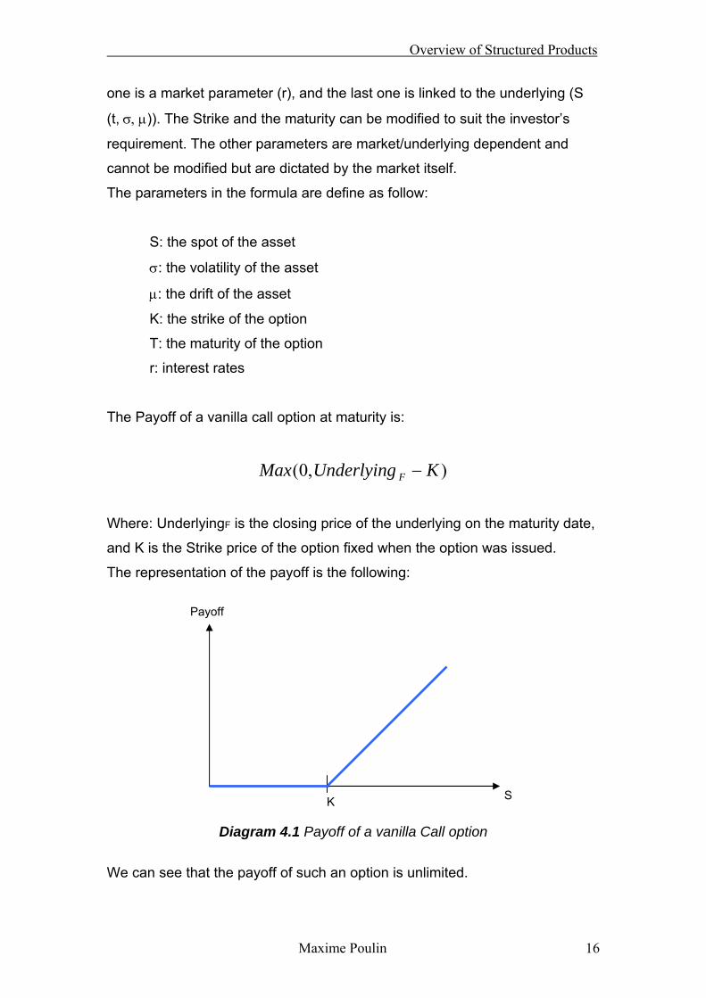
The Payoff of a vanilla call option at maturity is:
),0( KUnderlyingMax F −
Where: UnderlyingF is the closing price of the underlying on the maturity date,
and K is the Strike price of the option fixed when the option was issued.
The representation of the payoff is the following:
Diagram 4.1 Payoff of a vanilla Call option
We can see that the payoff of such an option is unlimited.
Payoff
K S
Overview of Structured Products
Maxime Poulin 17
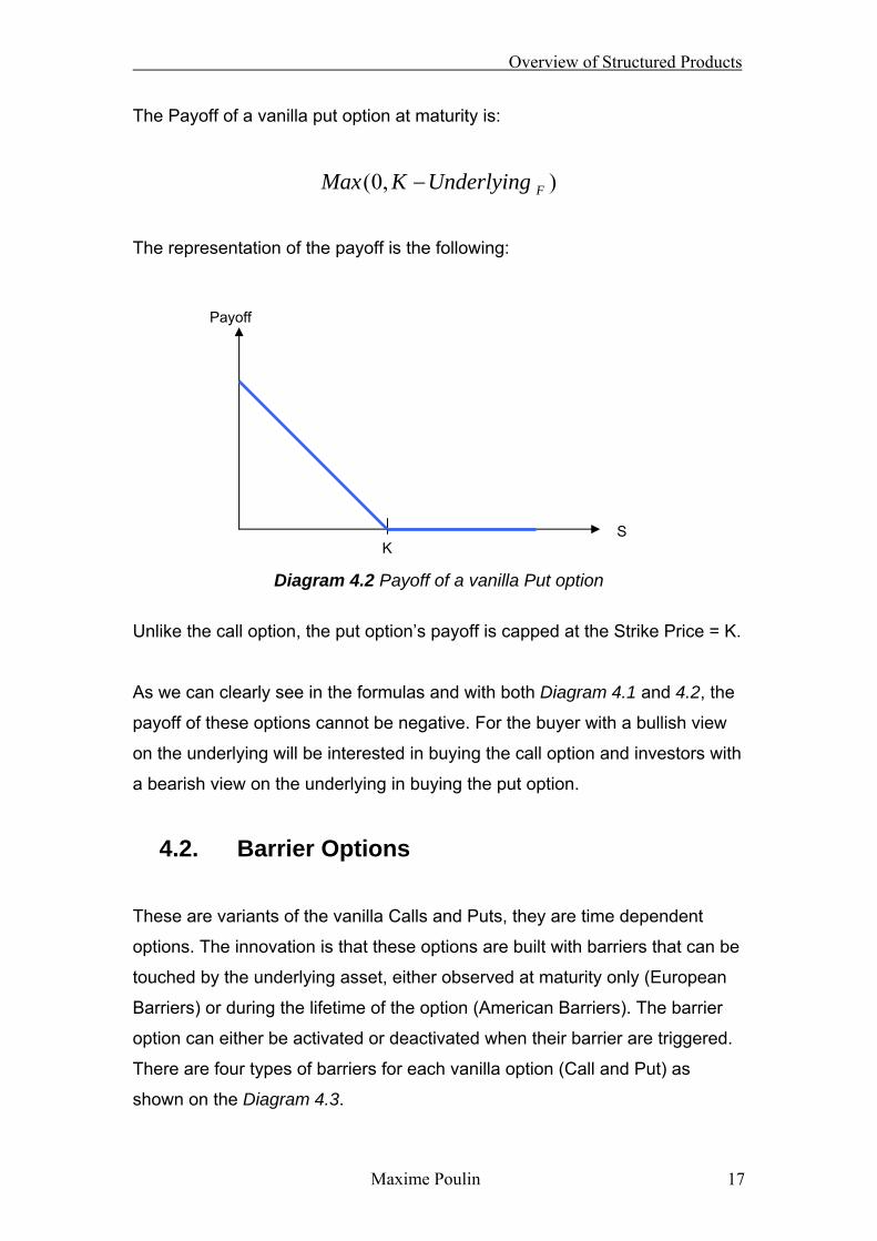
The Payoff of a vanilla put option at maturity is:
),0( FUnderlyingKMax −
The representation of the payoff is the following:
Diagram 4.2 Payoff of a vanilla Put option
Unlike the call option, the put option’s payoff is capped at the Strike Price = K.
As we can clearly see in the formulas and with both Diagram 4.1 and 4.2, the
payoff of these options cannot be negative. For the buyer with a bullish view
on the underlying will be interested in buying the call option and investors with
a bearish view on the underlying in buying the put option.
4.2. Barrier Options
These are variants of the vanilla Calls and Puts, they are time dependent
options. The innovation is that these options are built with barriers that can be
touched by the underlying asset, either observed at maturity only (European
Barriers) or during the lifetime of the option (American Barriers). The barrier
option can either be activated or deactivated when their barrier are triggered.
There are four types of barriers for each vanilla option (Call and Put) as
shown on the Diagram 4.3.
K S
Payoff
Overview of Structured Products
Maxime Poulin 18
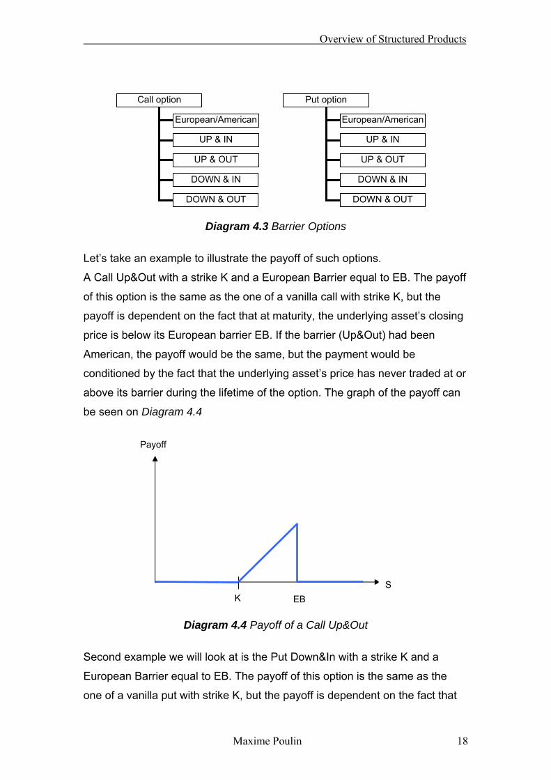
Diagram 4.3 Barrier Options
Let’s take an example to illustrate the payoff of such options.
A Call Up&Out with a strike K and a European Barrier equal to EB. The payoff
of this option is the same as the one of a vanilla call with strike K, but the
payoff is dependent on the fact that at maturity, the underlying asset’s closing
price is below its European barrier EB. If the barrier (Up&Out) had been
American, the payoff would be the same, but the payment would be
conditioned by the fact that the underlying asset’s price has never traded at or
above its barrier during the lifetime of the option. The graph of the payoff can
be seen on Diagram 4.4
Diagram 4.4 Payoff of a Call Up&Out
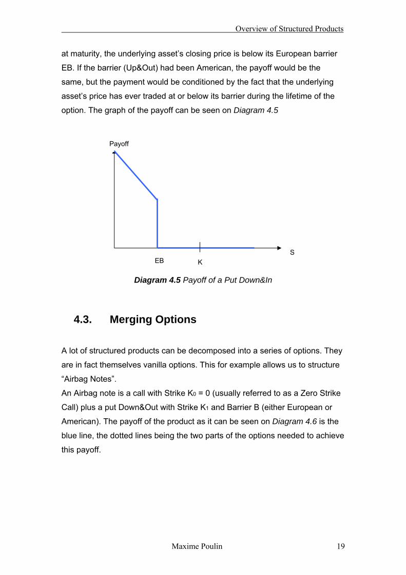
Second example we will look at is the Put Down&In with a strike K and a
European Barrier equal to EB. The payoff of this option is the same as the
one of a vanilla put with strike K, but the payoff is dependent on the fact that
Put option
European/American
UP & IN
UP & OUT
DOWN & IN
DOWN & OUT
Call option
European/American
UP & IN
UP & OUT
DOWN & IN
DOWN & OUT
Payoff
S K EB
Overview of Structured Products
Maxime Poulin 19
at maturity, the underlying asset’s closing price is below its European barrier
EB. If the barrier (Up&Out) had been American, the payoff would be the
same, but the payment would be conditioned by the fact that the underlying
asset’s price has ever traded at or below its barrier during the lifetime of the
option. The graph of the payoff can be seen on Diagram 4.5
Diagram 4.5 Payoff of a Put Down&In
4.3. Merging Options
A lot of structured products can be decomposed into a series of options. They
are in fact themselves vanilla options. This for example allows us to structure
“Airbag Notes”.
An Airbag note is a call with Strike K0 = 0 (usually referred to as a Zero Strike
Call) plus a put Down&Out with Strike K1 and Barrier B (either European or
American). The payoff of the product as it can be seen on Diagram 4.6 is the
blue line, the dotted lines being the two parts of the options needed to achieve
this payoff.
Payoff
S K EB

Overview of Structured Products
Maxime Poulin 20
Diagram 4.5 Payoff of an Airbag Note Many other payoffs can be manufactured from combining different vanilla options.
K1 K0 S
Payoff
B
Overview of Structured Products
Maxime Poulin 21
5. Black-Scholes Model
This model is the starting point of most other models in finance. It is also the
model the most widely used for pricing structured product, and is the
foundation of more complex models such as the Local Volatility Model (LVM).
5.1. Assumptions of the Black & Scholes model
The key assumptions made for the Black & Scholes to be correct are:
• The returns of the underlying follow a lognormal distribution with constant
drift µ and constant volatility σ
• It is possible to short (sell an underlying) in the market.
• There are no arbitrage opportunities in the market.
• Ability to trade the stock continuously.
• There are no transaction costs or taxes.
• All securities are perfectly divisible (e.g. it is possible to buy 1/10th of a
share).
• It is possible to borrow and lend cash at a constant risk-free interest rate.
5.2. Stochastic Differential Equations (SDEs)
These equations are separated in two parts: the Brownian element (which is
the stochastic element) and the Newtonian element (the deterministic term).
In finance we use the SDE with Ito’s lemma, which can be written as follow:
dWtXbdttXadX ),(),( +=

Overview of Structured Products
Maxime Poulin 22
5.3. Lognormal returns for asset prices
We assume (although it can be proved, but it is not the purpose of this paper)
that the returns of an asset are log normally distributed and answer to the
following rule:
tdWdtSdS σµ +=
Where
StXa µ=),( And
StXb σ=),(
5.4. The Black & Scholes formula
The Black & Scholes formula determines the variation of a derivative’s price
over time. It can be expressed with the following partial differential equation
(PDE).
rVSVrS
SVS
tV
−∂∂
+∂∂
=∂∂
2
222
21 σ
5.5. The Black & Scholes formulas for options
From the Black & Scholes formula, we can extract equation to express the
price of a call option and a put option. By expressing C the price of a call, P
the price of a Put, we can write the prices of each as an equation of the
Underlying price S, its volatility σ, the option strike K, its expiry T and the
interest rate r:
)()(),( 21 dNKedSNTSC rT−−=

Overview of Structured Products
Maxime Poulin 23
)()(),( 12 dSNdNKeTSP rT −−−= −
Where:
T
TrKS
dσ
σ⎟⎟⎠
⎞⎜⎜⎝
⎛++⎟
⎠⎞
⎜⎝⎛
=2
ln2
1
Tdd σ−= 12
N () is the cumulative distribution function of the standard normal distribution.
5.6. Call – Put Parity
This is a very important concept in finance; it is extracted from the Black and
Scholes formula. It gives us a linear relationship between the price of a put, a
call, a cash position and the underlying.
In order to show this relationship, we will proceed in two steps:
First we will consider the portfolio position of an investor at time T (portfolio
with Long/Short position)
Second we will take the present value of this portfolio by discounting it at the
risk free rate.
This present value will give us the Call – Put Parity.
Let’s assume the investor has the following portfolio:
a) He is long a cash position K
b) He is long a call strike K with expiry T
c) He is short a put strike K with expiry T
At maturity of the options (time T), the portfolio is worth:
Overview of Structured Products
Maxime Poulin 24
TT PCK −+=ΠT
But being long a call and short a put, means that the performance of the
Portfolio is exactly the same than the underlying. Moreover, the cash position
being equal to the strike of the option, the value of the portfolio at the expiry T
of the options is the value of the underlying.
TS=ΠT
From this, if we calculate the present value of the portfolio, we get:
0000 )()( SPCKPVPV T =−+=Π=Π
This gives us the following relation: the Call – Put Parity.
000)( PSCKPV +=+
Where:
Si is the spot price of the underlying at time “i”.
Ci is the price of call strike K with expiry T at time “i”.
Pi is the price of put strike K with expiry T at time “i”.
Πi is the value of the portfolio at time “i”.

Overview of Structured Products
Maxime Poulin 25
6. The Forwards
For all structured products, one need to understand the concept of forwards: it
is the expected value of the underlying at a point in the future.
This concept is used in most pricing of structured products.
Let’s see how to evaluate the forward of a security and how it varies over
time.
For this we will use the concept of lognormal distribution explained earlier:
tdWdtSdS σµ +=
If we assume that the Brownian term is null, we get the following equality:
dtSdS µ=
We can then easily solve this equation in order to get:
TqrT eSeSTS )(
00)( −== µ
We can see that the forward increases as interest rates increases and
decreases as dividends increases. This is a very important observation that
will be very useful when we’ll have to deal with the optimization problem.

Overview of Structured Products
Maxime Poulin 26
7. The Correlation
7.1. Definition
It is the linear relationship which exists between two random variables, or time
series. In other words a correlation ρ between a random variable X and a
random variable Y indicates the “probability” of X changing in a given direction
and in which direction for a given change in Y.
“Definition: The correlation can be seen as a strength vector between X and
Y, which expresses the intensity and the direction of their linear relationship.”
The correlation is a constant, and can be expressed as follow:
)()()()(
)()()()))(((),cov(2222 YEYEXEXE
YEXEXYEYXEYX
YX
YX
YX −×−
−=
−−==
σσµµ
σσρ
Where: ρ is the correlation between two random variables X and Y, with mean
µX and µY and standard deviation σX and σY. Cov () is the covariance and E ()
is the expected value.
Using Cauchy-Schwarz inequality we can show that the maximum value that
can take the correlation ρ is equal to 1.
7.2. Correlation term structure and skew
Empirically, it has been shown that the correlation between two assets is
mean reverting over time, and can be expressed as follow:
)(tρρ =

Overview of Structured Products
Maxime Poulin 27
It means that if we compare actual correlation to historical correlation, ρ(t)
should tend to the historical correlation over time.
Diagram 7.1 Correlation term structure
Moreover, correlation also depends on the market conditions. In a bullish
market, assets tend to have a smaller correlation whereas on a bearish
market, correlation between assets of the same asset classes tends to one.
This is referred to as the correlation skew:
)(Kρρ =
Diagram 7.2 Correlation Skew
As a conclusion, we can express the correlation as a function of time and
Strike:
),( Ktρρ =
Correlation
Maturity
Historical Correlation
Correlation
Strike

Overview of Structured Products
Maxime Poulin 28
8. Volatility and Variance
8.1. Definition
The volatility (σ the standard deviation) of an asset which return (as seen
earlier) are log normally distributed, is equal to the average change of the
value compared to its mean µ. The Volatility is defined as the square root of
the variance, where the variance of an asset A is defined as:
222 ))(()()))((()( AEAEAEAEAVar −=−=
And therefore
22 ))(()( AEAE −=σ
8.2. Implied Volatility
The implied volatility is defined as what the market thinks the volatility will be.
In order to evaluate this implied volatility, we will revert the Black & Scholes
formula. Meaning, we can get the option prices from the market, knowing
these, we will calculate the volatility implied by this option price using the
Black & Scholes formula.
But the Black & Scholes formula is very dependent on the dividends which
where used to price the option. In order to estimate the dividends traders tend
to use one of the following methodologies:
a) Using synthetic forwards (Long Call, Short Put)
Limitations: listed options are only liquid over a few years, to estimate
dividends over longer term; this method will not be accurate.
b) Extrapolate future dividends from recent dividends
Limitations: Past dividends do not always represent what will be paid in
the future.
Overview of Structured Products
Maxime Poulin 29
c) Follow analysts forecast.
Limitations: if the forecast is wrong, it will incur losses.
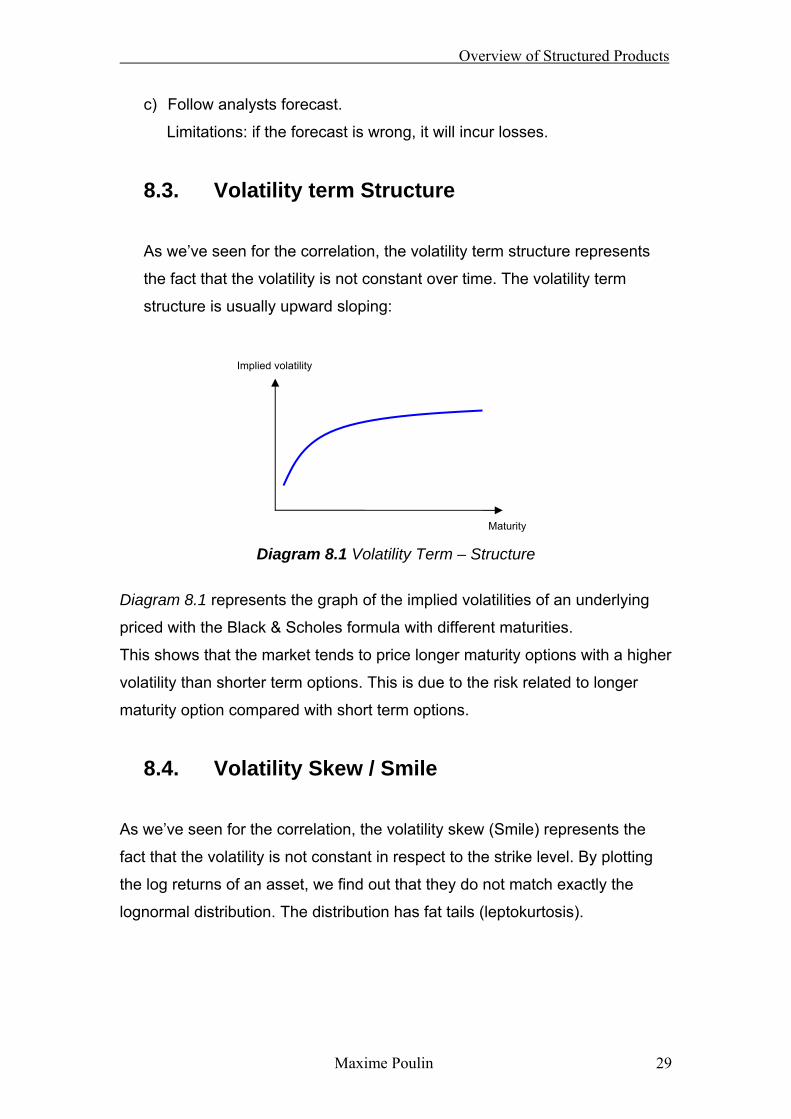
8.3. Volatility term Structure
As we’ve seen for the correlation, the volatility term structure represents
the fact that the volatility is not constant over time. The volatility term
structure is usually upward sloping:
Diagram 8.1 Volatility Term – Structure
Diagram 8.1 represents the graph of the implied volatilities of an underlying
priced with the Black & Scholes formula with different maturities.
This shows that the market tends to price longer maturity options with a higher
volatility than shorter term options. This is due to the risk related to longer
maturity option compared with short term options.
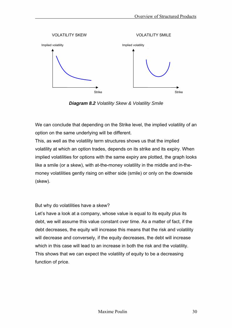
8.4. Volatility Skew / Smile
As we’ve seen for the correlation, the volatility skew (Smile) represents the
fact that the volatility is not constant in respect to the strike level. By plotting
the log returns of an asset, we find out that they do not match exactly the
lognormal distribution. The distribution has fat tails (leptokurtosis).
Implied volatility
Maturity
Overview of Structured Products
Maxime Poulin 30
Diagram 8.2 Volatility Skew & Volatility Smile
We can conclude that depending on the Strike level, the implied volatility of an
option on the same underlying will be different.
This, as well as the volatility term structures shows us that the implied
volatility at which an option trades, depends on its strike and its expiry. When
implied volatilities for options with the same expiry are plotted, the graph looks
like a smile (or a skew), with at-the-money volatility in the middle and in-the-
money volatilities gently rising on either side (smile) or only on the downside
(skew).
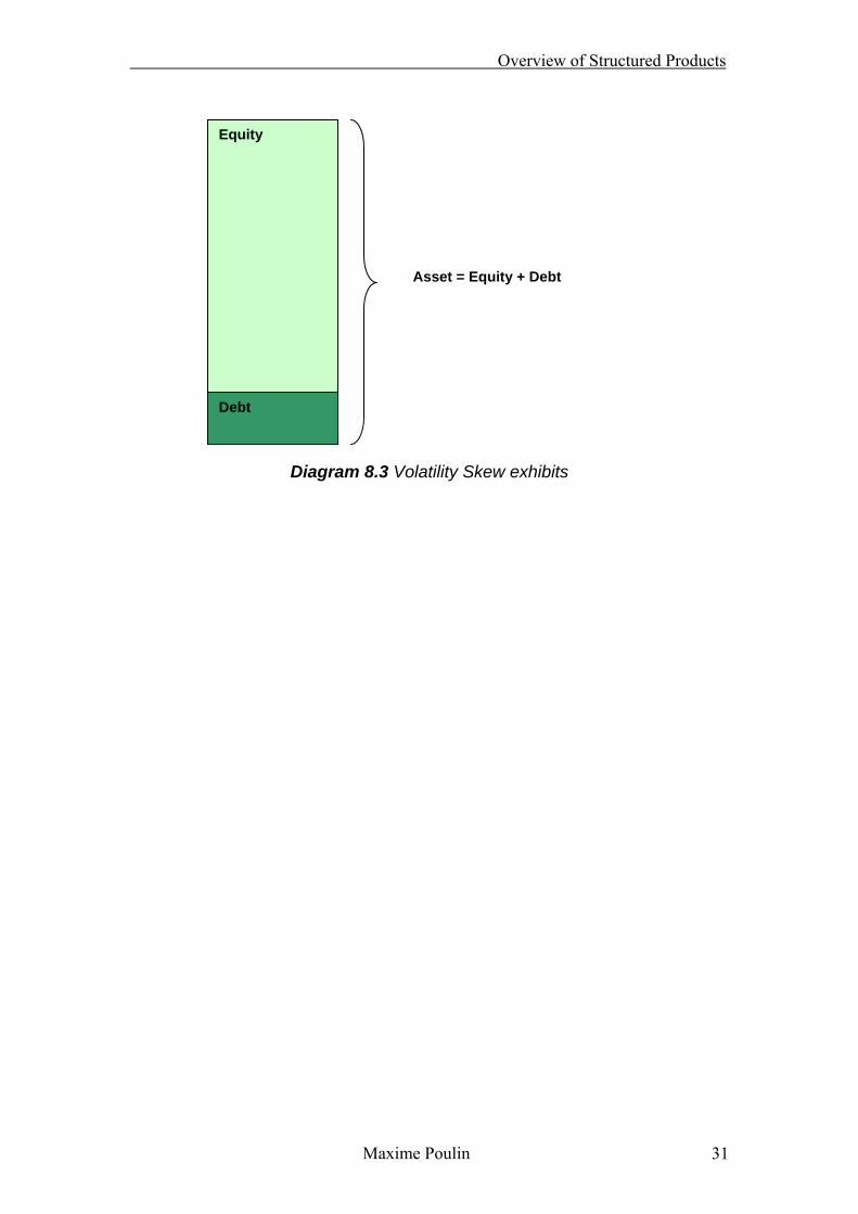
But why do volatilities have a skew?
Let’s have a look at a company, whose value is equal to its equity plus its
debt, we will assume this value constant over time. As a matter of fact, if the
debt decreases, the equity will increase this means that the risk and volatility
will decrease and conversely, if the equity decreases, the debt will increase
which in this case will lead to an increase in both the risk and the volatility.
This shows that we can expect the volatility of equity to be a decreasing
function of price.
Implied volatility
Strike
Implied volatility
Strike
VOLATILITY SKEW VOLATILITY SMILE
Overview of Structured Products
Maxime Poulin 31
Diagram 8.3 Volatility Skew exhibits
Equity
Debt
Asset = Equity + Debt
Overview of Structured Products
Maxime Poulin 32
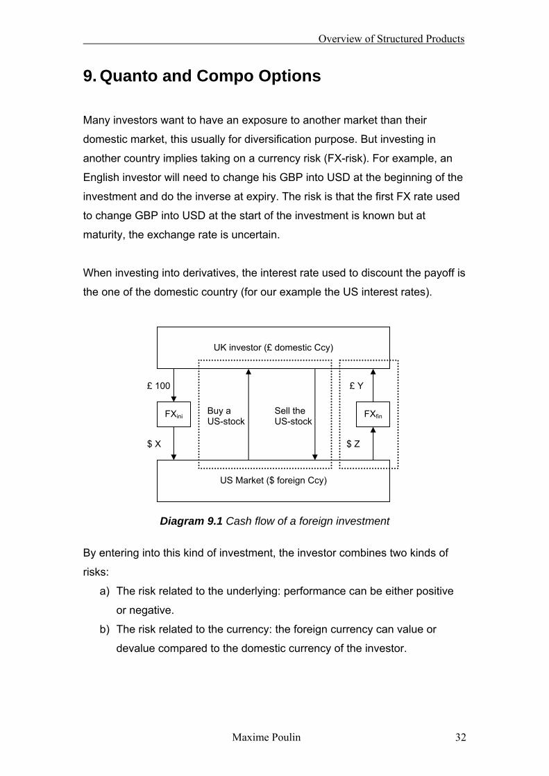
9. Quanto and Compo Options
Many investors want to have an exposure to another market than their
domestic market, this usually for diversification purpose. But investing in
another country implies taking on a currency risk (FX-risk). For example, an
English investor will need to change his GBP into USD at the beginning of the
investment and do the inverse at expiry. The risk is that the first FX rate used
to change GBP into USD at the start of the investment is known but at
maturity, the exchange rate is uncertain.
When investing into derivatives, the interest rate used to discount the payoff is
the one of the domestic country (for our example the US interest rates).
Diagram 9.1 Cash flow of a foreign investment
By entering into this kind of investment, the investor combines two kinds of
risks:
a) The risk related to the underlying: performance can be either positive
or negative.
b) The risk related to the currency: the foreign currency can value or
devalue compared to the domestic currency of the investor.
UK investor (£ domestic Ccy)
US Market ($ foreign Ccy)
£ 100
Buy a US-stock
FXini
$ X
Sell the US-stock
£ Y
FXfin
$ Z
Overview of Structured Products
Maxime Poulin 33
Compo Options “Definition: Derivatives where the payoff (expressed in foreign currency) is
converted back into the domestic currency with the exchange rate at maturity
and discounted with the domestic discount factor.”
Compo option transfer all the FX-risk to the investor, but some investors might
have a conflicting view between the Underlying and its currency.
An alternative to these options are the Quanto Options.
Quanto Options “Definition: Derivatives where the payoff (expressed in foreign currency) is
converted back into the domestic currency with a pre-specified exchange rate
at maturity and discounted with the domestic discount factor.”
Pricing quanto options:
If we assume that the exchange rate (FXt exchange rate at time t) log-normal
distributed stochastic process, we have:
FXFXfdt
t dWdtrrFXdFX
σ+−= )(
Where rd is the risk free rate of the domestic country, rf is the risk free rate of
the foreign country, σ is the volatility and dW is the Wiener process.
As we’ve seen earlier we have the same relation for the underlying’s price in
its home currency:
SSdt
t dWdtdrSdS σ+−= )(
Where d is the dividend rate of the underlying.

Overview of Structured Products
Maxime Poulin 34
The actual forward will be written as follow:
TdrrTdrT SFXfdd eSeSeSTS )(
0)'(
00)( σσρµ ⋅⋅−−−− ===
The option will then be price as seen earlier with this adjusted forward.
Overview of Structured Products
Maxime Poulin 35
10. Sensitivities of Exotic Options
This is used by all traders in the pricing stages to evaluate risks: there are two
ways to find these sensitivities; both are to be used simultaneously in order to
allow crosschecks:
a) Pragmatic approach: Estimating how the probability of being in or out
of the money will vary.
b) Mathematical approach: by isolating each parameter and looking at
the impact of a small change in this on the price of the derivatives.
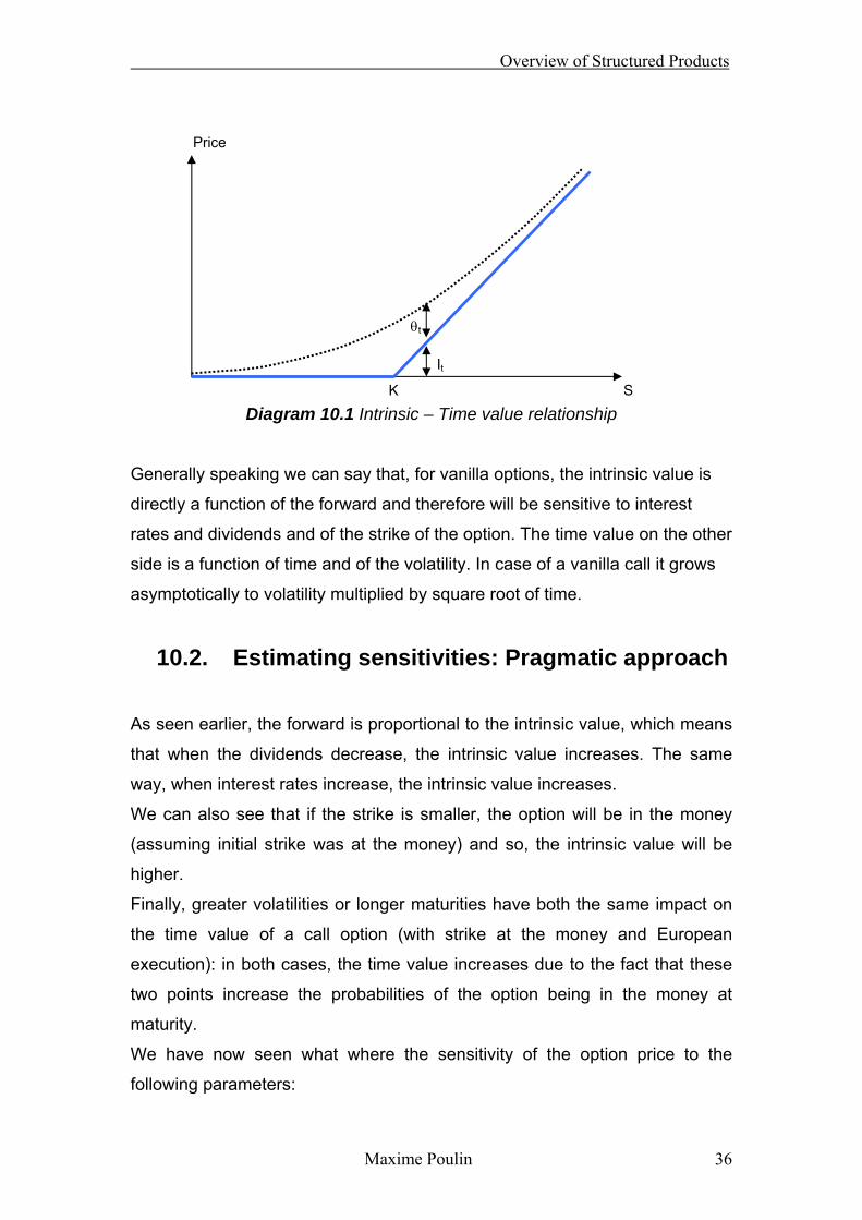
10.1. Time Value Relationship
We know that at maturity, the value of the call option is equal to its payout (the
blue line in Diagram 4.1), let’s take the example seen before: call with strike K
and maturity T with a European type exercise.
( ) ),0(TC KUnderlyingMax F −=
The value of a call option at any time t can be decomposed into two elements:
a) The intrinsic value It. Is the value the option would have if exercised at
a time t; it corresponds to the payout a similar option but with expiry t
would have.
b) Its time value θt. This is the term valuing the probability of being in the
money at maturity.
The Intrinsic – Time value relationship for a call C at time t expresses the
value of the option at that time and can be written as:
( ) ( )tθ0,maxθIC ttt +−=+= KUnderlyingt
Overview of Structured Products
Maxime Poulin 36
Diagram 10.1 Intrinsic – Time value relationship
Generally speaking we can say that, for vanilla options, the intrinsic value is
directly a function of the forward and therefore will be sensitive to interest
rates and dividends and of the strike of the option. The time value on the other
side is a function of time and of the volatility. In case of a vanilla call it grows
asymptotically to volatility multiplied by square root of time.
10.2. Estimating sensitivities: Pragmatic approach
As seen earlier, the forward is proportional to the intrinsic value, which means
that when the dividends decrease, the intrinsic value increases. The same
way, when interest rates increase, the intrinsic value increases.
We can also see that if the strike is smaller, the option will be in the money
(assuming initial strike was at the money) and so, the intrinsic value will be
higher.
Finally, greater volatilities or longer maturities have both the same impact on
the time value of a call option (with strike at the money and European
execution): in both cases, the time value increases due to the fact that these
two points increase the probabilities of the option being in the money at
maturity.
We have now seen what where the sensitivity of the option price to the
following parameters:
S
Price
K
θt
It

Overview of Structured Products
Maxime Poulin 37
a) Dividends
b) Interest Rates
c) Strike
d) Volatility
e) Maturity

Overview of Structured Products
Maxime Poulin 38
11. Models used on Trading floors (Commerzbank)
There is a great variety of models used in finance in order to price derivatives.
They range from the Black & Scholes model to the stochastic volatility model.
But why do we need so many different models to price structured products?
How should we be able to choose which model will be the most accurate for a
specific structure?
Models in finance are mathematical tools and in the same way than
mathematical models are used in finance, each one has been implemented
for a specific purpose and to work on specific element (whether on a finance
or physics related subject).
What is a model?
A model is a series of laws which have been derived from empirical
observations and which have to describe and predict a given process in the
best possible way.
The options prices do not have a linear behavior; their first order derivative
with respect to a given parameter is not equal to zero. This has an important
impact on the option pricing.
When the second order derivative is negligible, a simple model will be enough
to price the option: in most case, a vanilla product (for example, the Black &
Scholes model will suffice).
When the first order is not enough and we have to take into consideration the
second order derivative because its impact on the option price is important.
As we’ve seen in part 5, the Black and Scholes model assumes that volatility
is constant. But like we said in part 8, it is not the case for assets in the
market, there is a skewed behavior of lognormal returns. Since skew does not
affect vanilla options with strike at the money and European execution, they
Overview of Structured Products
Maxime Poulin 39
can be priced with the Black & Scholes model. But if the strike of the option is
not at the money, we will need to use a model which estimates correctly the
impact of the skew.
This leads us to the conclusion that before choosing which model to use to
price an option, we need to check what parameter will have an impact on the
value of the option in order to have a model which will model correctly the
relevant parameter, so that the value of the option will be correct.
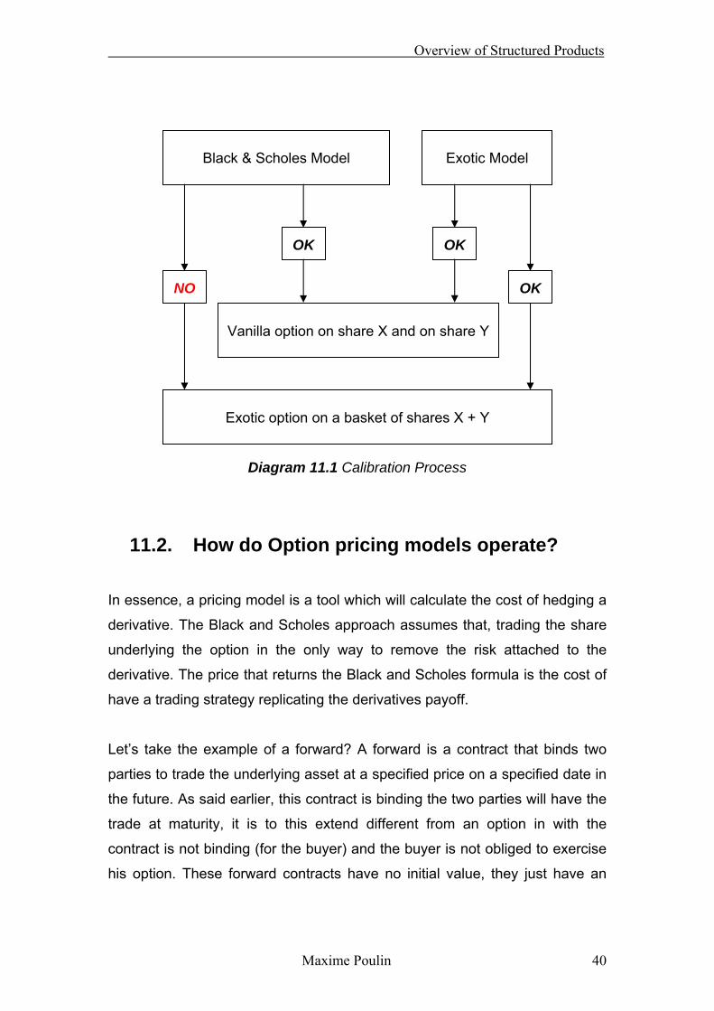
11.1. Calibration process of a model
This process is essential in order to get a correct price for an option.
We will focus our explanation around an example.
If we had to price an exotic barrier option, where the underlying is a basket of
shares (X and Y). As we’ve seen earlier, the Black & Scholes model won’t be
suitable for such an option; therefore, we’ll need to use a more complex
model. This model has to give the exact same price than the Black & Scholes
model for the individual at the money vanilla options. Adapting the parameters
of the model so that these points are matched is known as the “calibration
process”.
Overview of Structured Products
Maxime Poulin 40
Diagram 11.1 Calibration Process
11.2. How do Option pricing models operate?
In essence, a pricing model is a tool which will calculate the cost of hedging a
derivative. The Black and Scholes approach assumes that, trading the share
underlying the option in the only way to remove the risk attached to the
derivative. The price that returns the Black and Scholes formula is the cost of
have a trading strategy replicating the derivatives payoff.
Let’s take the example of a forward? A forward is a contract that binds two
parties to trade the underlying asset at a specified price on a specified date in
the future. As said earlier, this contract is binding the two parties will have the
trade at maturity, it is to this extend different from an option in with the
contract is not binding (for the buyer) and the buyer is not obliged to exercise
his option. These forward contracts have no initial value, they just have an
Black & Scholes Model
Vanilla option on share X and on share Y
OK
Exotic Model
Exotic option on a basket of shares X + Y
OK
OK NO
Overview of Structured Products
Maxime Poulin 41
execution price, price at which the underlying asset will be exchange at
maturity, and there is no upfront payment.
In order to hedge his risk, the seller of this kind of contract can for example
buy the underlying asset right now and hold it until the delivery date of the
contract, in this case the hedge is perfect, there is no more risk, and the
outcome is known with certainty.
From that, how can we estimate the settlement price, in other words the fair
price of this contract to buy / sell the underlying asset in the future, so that no
upfront is needed for the transaction? As we’ve seen in order to hedge this
position, we would need to buy the underlying asset now at a known price.
But there is a cost of financing, borrowing the cash in order to buy the
underlying asset is worth the interest rate paid during the holding period. The
full hedging cost in then equal to the price of the underlying asset plus the
borrowing cost incurred to buy the share and hold it until maturity.
As an example, assume that the underlying asset’s price is GBP 100, the
contract’s maturity is 1 year, and the interest rates are at 2%p.a. The one year
forward selling price of the underlying asset is GBP 102, which is as explained
earlier, the price of the asset (i.e. GBP 100) + the cost of borrowing GBP 100
over one year (i.e. GBP 2). At the end of the period, the seller of the contract
will have a flat position: no profits and no losses will impact him wherever the
underlying asset’s price goes.
If the agreed settlement price for the forward contract (referred to as the Strike
price) is not exactly equal to GBP 102, one of the parties will have to pay an
amount upfront to the other in order to compensate the difference.
The GBP 102 is not an arbitrary number but is the actual cost of delivering a
share worth GBP 100 today in one year knowing that the interest rates are at
2.00%, meaning that the holding cost will be of GBP 2.00.

Overview of Structured Products
Maxime Poulin 42
If the buyer has a right to cancel the contract, the pricing of such a contract
becomes entirely different. The simple hedging strategy described above
won’t be possible anymore, because if at maturity the underlying asset’s price
is below the strike price, the buyer of the contract won’t be willing to settle the
transaction as he would be better of buying the stock directly in the market at
the current market price. This would leave the seller short cash (GBP 102)
and long the stock (worth less than GBP 102), which would incur a loss. This
would not be acceptable. One possible strategy would be to sell the
underlying asset when its price falls below the strike price of the contract, and
buy it when its price goes back above the strike price. Another would be to
“smooth” the trading, by buying half a share initially, assuming that it is about
equally likely that the share is going to go up as down, and buying or selling
another half share at some point in the future depending on the way in which
the price moves.
If we consider a simplified market, with a binomial tree for the share price at
maturity: it can be GBP 95 or GBP 105. In this market, interest rates are
assumed to be equal to 0. The strike price of the option is GBP 100. In order
to hedge, the seller of the contract buys half a share on the start date of the
contract. At maturity, if the underlying’s price is GBP 105, then, the seller is
long half a share worth GBP 52.50 for which he spent GBP 50, but he will
need to buy another 50% of a share has he has to deliver one share. Buying
another 50% of a share worth GBP 105, will cost him GBP 52.50. In the end
the seller will have lost GBP 2.50.
If the share price drops, the seller of the option is left holding half a share,
worth GBP 47.50, for which he paid GBP 50. The buyer is not interested in
the option has the strike price is above the spot price. So the seller will have
to liquidate his position at a loss of GBP 2.50.
We can see that this hedge as a fixed cost of GBP 2.50 for the seller
whatever the scenario is. By charging GBP 2.50 upfront to the buyer, the
seller hedges his risk and has a flat position again. We can conclude that with
these market conditions, the fair price for this option is GBP 2.50.
Overview of Structured Products
Maxime Poulin 43
But with the actual market conditions, there are a much more possible
outcome than a simple binomial tree, which is why we need more complicated
model in order to take into account all these parameters with assumed
negligible the simplified explanation given previously.
An important point about the hedging strategy in the simplified market model
is that it involves buying shares at a higher price than they are sold. This is
what incurs a loss for the seller, and this is why an option is not worth zero. In
other words, all models will estimate the loss incurred by the hedge which will
require of the seller to buy high and sell low. This also implies that the seller
when he gives an estimation of the hedging cost does not care where the
stock price will eventually go, his concern is to cover the potential outcome
regardless of their probability with the model.
Black & Scholes option pricing is therefore just a complicated way of working
out the loss from running a hedging strategy like the ones described above,
which systematically buys shares at a higher price than they are sold. The
model makes assumptions about how the share price behaves in the very
short term, and then adds up the effect of these very short term moves,
combined with the hedging strategy which specifies how many shares are
actually being held at any time, to calculate the losses that arise from the buy
and sell strategy. The borrowing cost: financing cost is also taken into
consideration in all financial models.
The innovation that Black & Scholes brought was that it offered an accurate
representation of the market movements. Moreover, it includes a hedging
strategy which offer a perfect solution for the option seller if the market
behaves as the model expect it to behave in it representation. In other words,
the person doing the hedge will be completely indifferent to the direction the
underlying asset price takes. But one of the draw backs is that the Black &
Scholes model will only model the short term movements of an underlying
asset price but will not make any assumption over the long term.

Overview of Structured Products
Maxime Poulin 44
For highly volatile underlyings, the losses incurred by the Buy High Sell Low
strategy are much higher than what they would be with less volatile
underlyings. This explains why the price of vanilla option is highly dependent
on the volatility of the underlying asset.
As we’ve just seen, simple derivative pricing tools assume that the
underlying’s price is continuously moving, the models are representing this
movement over a short tem period. For the particular case of the Black &
Scholes model, the distribution of the underlying price and the size of the
spread is dependent on two factors: the volatility of the stock (a constant), and
the time over which the changes are observed (the exact relation is with the
square root of this duration). This model also assumes that upward movement
are as probable and are of the same size than downward movement of the
stock price. One of the problems of this model is that it considers the volatility
is constant over time which as we’ve seen earlier is not the case.
Solving the Black & Scholes formula tells us that the fair price of an option is
the weighted (by their probabilities) average of all the possible payoffs of the
option at maturity. With this method, the option fair value is the same when
calculating the losses incurred by the hedge over the life of the option and
calculating the average option price given the final distribution of the returns of
the underlying at maturity obtained through the model which return a short
term representation of the underlying asset price evolution.
In order to avoid having to simulate the entire path of an underlying from the
issue date to the maturity date, Monte-Carlo simulations are taking advantage
of this point, by only simulating changes from issue date and maturity date
and not looking at the changes in between. This gives us the distribution of
the prices at the end of the period which is the same than the one of the
prices we would get if the underlying asset price follows the exact path
modelled with the Black and Scholes equation. The model will estimate the
payoff of each path simulated with the Monte-Carlo. The fair value of the
option can be calculated by taking the weighted (by their probabilities)
average of all these payoffs (discount with the actual interest rates).

Overview of Structured Products
Maxime Poulin 45
But in the market, we can observe that option have a skew / smile, which are
not taken into consideration by the Black & Scholes model as explained
earlier on, this, implies that the price give by this model is not completely
accurate. The conclusion we can take out from this is that due to the skew
and smile, the returns are not log-normally distributed.
But as we said for Monte-Carlo simulation, the path followed by the underlying
asset between the issue date and the maturity date is not relevant for the
evaluation of the option price. As a matter of fact, the return not being log-
normally distributed is not important. If the distribution of returns can be
estimated, a Monte-Carlo simulation accounting for the skew will be possible.
For path dependent option, this pricing method will not work (for example an
American barrier option or an Asian option).
11.3. Black Vanilla Model
It is considered as one of the simplest models, but can only be used for
analytic pricing of vanilla options.
It cannot be used to price more complex structures in which a splife of the
payoff would be needed (Monte-Carlo simulations are not possible with this
model).
11.4. Black Diffusion Model
This model is the simplest model which can be used with a Monte-Carlo
simulation. It takes into account the term-structure for each underlying but
does not account for the skew.
Products which require a splife for their payoff can be priced with this model,
but the impact of the skew will not be taken in to account. As the impact is
very significant on a number of structured products, this model is not the one
which is the most often used.

Overview of Structured Products
Maxime Poulin 46
11.5. Local Volatility Model
Local volatility is a simple concept which says that the instantaneous volatility
of the process which drives share price changes is a fixed function of time and
the actual share price. If we assume the Local Volatility rules apply, we should
be able to know the volatility of a stock at any point in the future for any given
point time and underlying share price.
By looking at the options (vanilla) quoted on the market, we can create a
matrix of the short term volatilities (a volatility surface) depending on the time
and the underlying’s share price. With this matrix Monte-Carlo simulation can
easily by done as short term variations of the price can be evaluated with the
matrix. But regarding longer term variations, the model is much slower as the
calibration process takes a long time, and the need to calculate paths with
many intermediate observation dates and not just the actual ones impacting
directly the payoff of the derivative.
Although used in Commerzbank, the Local Volatility model is widely used in
finance to price options: either with an immediate starting point but also with
forward starting date. There are some known problems with the so-called
“dynamics” of the implied volatility with this model, but it is a very powerful and
widely used model which is the benchmark for most pricing.
11.6. Stochastic Volatility Model
This model is a variation of the Local Volatility model which attempts to
reduce the problems of the implied volatilities “dynamics” as well as the
limitation due to the assumptions that volatility is only a function of the spot
price of the underlying and the time. But as it can easily be observed in the
market, this assumption is erroneous.
Overview of Structured Products
Maxime Poulin 47
This can be very important in pricing certain types of option which have “Vega
convexity”. This means that their sensitivity to implied volatility is not constant,
and as implied volatility goes up and down, so will the sensitivity to this
parameter. Imagine a situation where an exotic option which has a positive
sensitivity to implied volatility is Vega-hedged with a vanilla option. If the
exotic option has “positive” convexity of Vega, then its sensitivity to implied
volatility increases as implied volatility increases. So the total position will no
longer be hedged if implied volatility goes up, as the exotic option will have
become more sensitive. The hedger will need to sell some more vanilla
options in order to have a hedged position again. If implied volatility then
drops, the hedger will have to unwind the vanilla option trade. They will make
money on this unwind, as they are buying back the vanilla option at a lower
level of implied volatility compared to the level at which they bought it. So a
positive Vega convexity position will consistently make the holder money
when implied volatility varies itself.
The problem arises where an exotic option position has negative Vega
convexity. The holder of such a position will systematically lose money if
implied volatility changes, and this clearly happens on a daily basis in the
market. So they need a model to calculate the cost of these changes, in just
the same way that the basic Black & Scholes model calculates the cost of re-
heding the delta of an option.
Stochastic volatility models generally have five components. The average
level of the basic volatility of the share price, the volatility of this volatility
(which can be seen as the acceleration), the correlation between the basic
volatility and the “acceleration”, and the speed to which the basic volatility
reverts to its mean level. (This mean reversion is necessary as it is clear that,
unlike a share price, implied volatility does not increase without limit. A share
price can double, triple, quadruple or even more, whereas volatility cannot
increase above a certain level, except for very short periods.)
This is why stochastic volatility models are used to price options with Vega
convexity. The classic example of an options with Vega convexity are certain
Overview of Structured Products
Maxime Poulin 48
types of cliquet option, often called “best-of ratchets” or “reverse cliquets” or
“napoleons”. Note that there is a common mistake that it is the forward-
starting nature of these options than means they have to be priced with
stochastic volatility models. This is not true; it is the fact that they have strong
Vega convexity. Other types of options, for example simple barrier options,
can also have strong Vega convexity. It is even possible to construct a
portfolio of vanilla options (the “butterfly strategy”) which has strong convexity.
However with the vanilla options, the convexity cost of the strategy is
accounted for in the shape of the volatility surface.
The mathematical characteristics of stochastic volatility models are the
following:
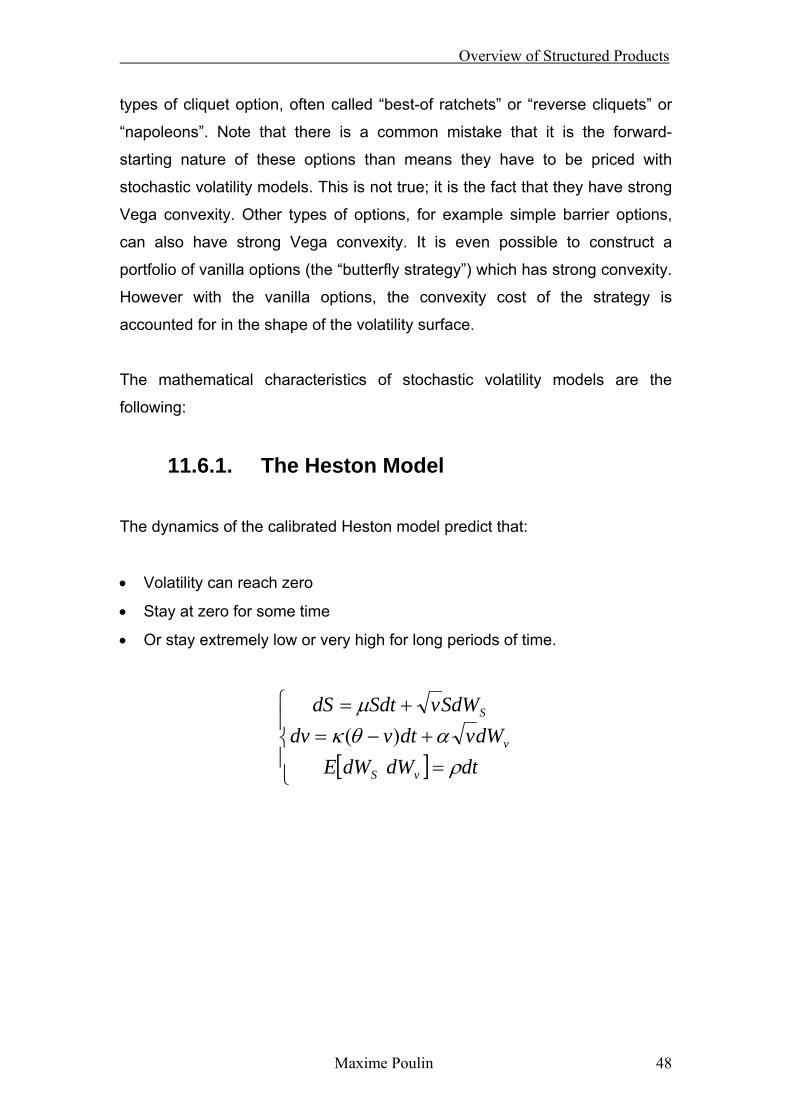
11.6.1. The Heston Model
The dynamics of the calibrated Heston model predict that:
• Volatility can reach zero
• Stay at zero for some time
• Or stay extremely low or very high for long periods of time.
[ ]⎪⎩
⎪⎨
⎧
=+−=
+=
dtdWdWEdWvdtvdv
SdWvSdtdS
vS
v
S
ραθκ
µ)(
Overview of Structured Products
Maxime Poulin 49
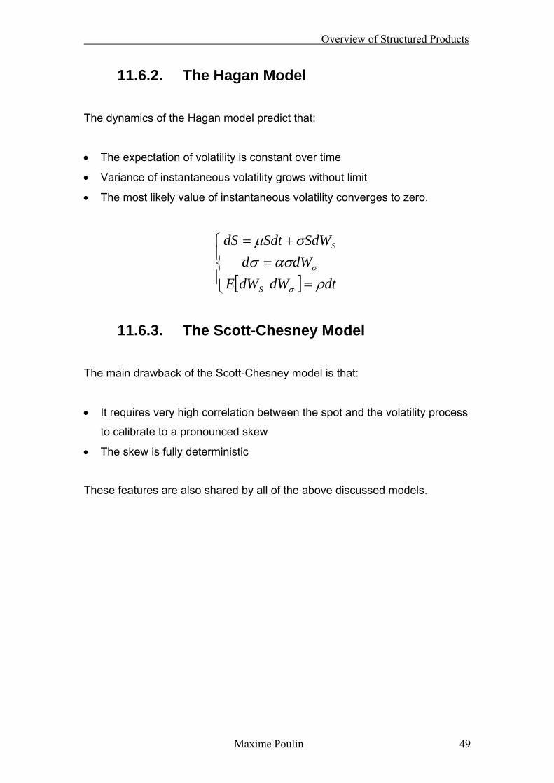
11.6.2. The Hagan Model
The dynamics of the Hagan model predict that:
• The expectation of volatility is constant over time
• Variance of instantaneous volatility grows without limit
• The most likely value of instantaneous volatility converges to zero.
[ ]⎪⎩
⎪⎨
⎧
==
+=
dtdWdWEdWd
SdWSdtdS
S
S
ρασσ
σµ
σ
σ
11.6.3. The Scott-Chesney Model
The main drawback of the Scott-Chesney model is that:
• It requires very high correlation between the spot and the volatility process
to calibrate to a pronounced skew
• The skew is fully deterministic
These features are also shared by all of the above discussed models.

Overview of Structured Products
Maxime Poulin 50
12. The risks related to structured products
When a bank issues a structured product to a client, it is in fact selling a
contract (under form of swap, note or certificate) that ensures the holder
receives a given percentage of the notional invested back, depending on the
performance of the underlying asset(s). The role of the trader is to ensure that
the right amount of risk is always hedged away in order to be able to fulfil the
conditions stated in the contract.
Due to the complexity of the financial world, and especially that of exotic
products, the hedges are far from being completely accurate. This is often not
related to the ability of the trader but rather to the nature of risk which has to
be hedged away.
It is possible to categorize the main risks into the following sub-categories:
a) Delta risk
b) Vega risk
c) Correlation risk
d) Second order risks
The value of an option can vary over time because of several market
parameters. The trader has to have an opposite position in the market (with
respect to the issued products) in order to reflect the change in value of the
derivative instruments. The main components which have to be hedged away
are the so-called first-order risk indicated above (Delta, Vega and
Correlation). Once these have been hedged, the trader has still to verify the
presence of second order risk like Volga or Vanna. Usually their effect is
negligible for vanilla options and most of the commonly traded exotic options.
But this is not the case for cliquets and other unusual exotic payoffs.

Overview of Structured Products
Maxime Poulin 51
12.1. Delta Risk
The Delta represents for the trader, without any doubt, the most important risk
to be hedged. This is achieved by buying (or selling) the right amount of
shares (futures contracts in case of indices) in order to have at all time (or as
many time as possible) a flat delta position. In other words the trader has to
be long (or be short) at any time an amount of the underlying asset so that if
added to its delta position, resulting from the products issued, equals zero.
Liquidity is in this case a very important aspect which has to be analyzed
when checking if a given underlying can be hedged or not. It is important to
verify that the amount of shares traded per day corresponds to the delta of the
product which has been sold since the trader, as stated previously, has to buy
(or sell) exactly that amount of shares.
12.2. Vega Risk
Once the Delta component is hedged away, the trader still has the risk
associated with the volatility of the underlying.
Suppose that a bank sells an at the money call option on one underlying
today to one of its clients. This option has a value A which can be estimated
with the Black & Scholes equation as previously seen.
Suppose that after a period t, the market has not moved compared to the
issue date, meaning that all the market parameters have remained constant
over time. The value of the option has therefore not changed (if we neglect
the time decay) and the call is still worth A. Suppose now that after the period
t, all the market parameters have not seen any change but the volatility of the
underlying (on which the option is based) has increased. The option is now
worth B (where B is greater than A since a call is long Vega). In order to be
hedged, the trader has, therefore, to buy volatility, i.e. he will buy option on
this underlying.

Overview of Structured Products
Maxime Poulin 52
12.3. Correlation Risk
Correlation risk is one of the most important and dangerous component to
which banks are exposed. Due to the nature of the products sold over the
past decade, banks are generally short on correlation. This is because of the
attractiveness nature of low correlation. Let’s have a look at a generic product:
the “worst of”, meaning that the payoff, usually represented by a big coupon
or the capital protection, depends on event that one (or more) of the N
underlyings has touched a barrier or not. The lower the correlation the more
attractive the final payoff will be for the investor.
Consider a reverse convertible worst of where, at maturity, the investor is long
a bond, receives a coupon X and is short a put down and in (with barrier B) on
the worst performing stock. He receives therefore his notional back plus the
coupon X if none of the underlying stocks ever traded below B. In case the
condition is not verified, and therefore one or more stocks did trade below the
barrier B, the client still receives the coupon X, but the notional invested is
reduced by an amount corresponding to the highest drop among the stocks at
maturity. In order to have an attractive coupon it is in the investor’s interest to
choose stocks with as low correlation as possible. By reducing the correlation
we increase the probability of one of the shares touching the barrier B. This
will, in turn, increase the probability of losing the capital protection at maturity,
leaving more to spend for the coupon X.
12.4. Second order Risks
Modelling risk refers to the model used to evaluate the price of the derivative
instrument. Due to the complexity of exotic products it is crucial to take into
account all the effects that could affect their value. There are products for
which second order effects (second order derivatives with respect to a given
market parameter) do not have to be taken into account. This is especially the
case for simple products like vanilla options or even simple exotic options.

Overview of Structured Products
Maxime Poulin 53
Consider, for example, an at-the-money call option on a given underlying
asset. This option can be valued with the Black-Scholes model or with the
more “sophisticated” Local Volatility Model and the price we would get would
be exactly the same. Skew effects have, in fact, no influence when valuating
an at-the-money vanilla call option.
Consider now a barrier option, like a down-and-out put option with barrier at
60%. The model used in this case assumes a very important role. The Black-
Scholes model would use the same volatility for the strike and for the barrier,
whereas the Local Volatility Model would consider two different volatilities
because of presence of skew.

Overview of Structured Products
Maxime Poulin 54
13. Example of exotic derivative: Cliquets
A cliquet, ratchet option or strip of forward start options is a derivative where
the strike is reset on each observation date at the then current spot level. The
profit can be accumulated until final maturity, or paid out at each observation
date.
Cliquets are complex exotic products where second order effects can
significantly affect the pricing. There are two main effects which have to be
considered:
a) Volatility of volatility effects (Vega convexity)
b) Forward skew effects
Not all cliquets are sensitive to volatility of volatility (“acceleration”) and
forward skew. We’ll see what the impact is on the main types of re-striking
options.
13.1. Convexity (or Volga)
Let’s consider an ATM European call option. We have seen that its price can
be written as
TC **4.0 σ≈
If we draw the price of this option with respect to the volatility we can see that
it is a straight line with positive slope, as shown in Diagram 13.1.

Overview of Structured Products
Maxime Poulin 55
Diagram 13.1 A call option price as a function of volatility
It is easy to verify that the Vega in this case is equal to a constant, because
we have a linear relationship; it is therefore independent from the level of the
volatility. The Vega is a constant line as shown in Diagram 13.2.
Diagram 13.2 A call option’s Vega as a function of volatility
So for an ATM call
0Volga 2
2
=∂∂
=σV
Sigma
Price
Sigma
Price
Overview of Structured Products
Maxime Poulin 56
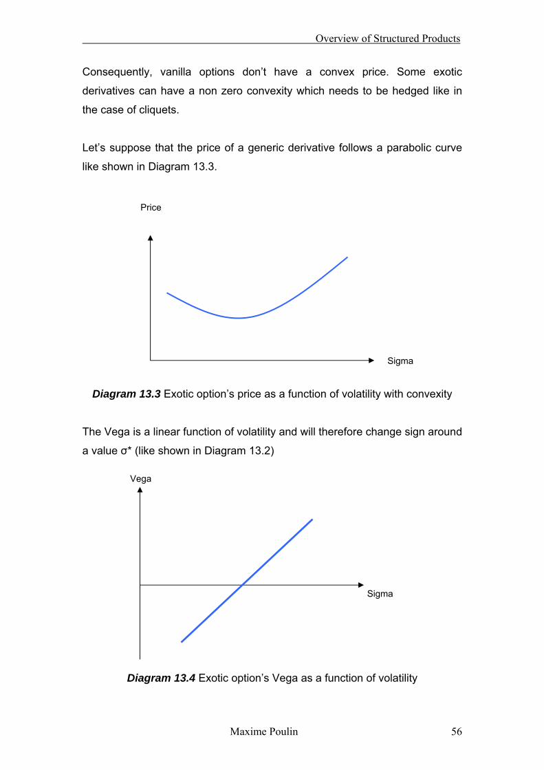
Consequently, vanilla options don’t have a convex price. Some exotic
derivatives can have a non zero convexity which needs to be hedged like in
the case of cliquets.
Let’s suppose that the price of a generic derivative follows a parabolic curve
like shown in Diagram 13.3.
Diagram 13.3 Exotic option’s price as a function of volatility with convexity
The Vega is a linear function of volatility and will therefore change sign around
a value σ* (like shown in Diagram 13.2)
Diagram 13.4 Exotic option’s Vega as a function of volatility
Sigma
Price
Sigma
Vega

Overview of Structured Products
Maxime Poulin 57
As you can see in this case, the Vega is not constant with respect to volatility
but is a linear function of the volatility. We call σ* the volatility where the Vega
is equal to zero and change sign. If we are buying volatility, the more σ
increases, the smaller the Vega is. In order to hedge our position, we need to
buy the volatility, therefore we buy the volatility when it increases and we sell
it when it decreases. This hedging cost has therefore to be included in the
price of the derivative. Finally when the Volga is non zero, we are dealing with
the volatility of the volatility, so we need to consider a stochastic volatility, and
use a stochastic volatility model to price the derivative.
13.2. Cliquets
There are various types of cliquets options and an extensive list would not be
possible. We’ll present only the main typologies since the effects which have
to be taken into account are common to all of them.
13.2.1. Classic Cliquet
The classic cliquet is a forward starting option, which fixes its strike at time t
(from today) and expires at time T (from today). For a cliquet call option the
payoff would be:
⎟⎟⎠
⎞⎜⎜⎝
⎛−= 1,0
t
TT S
SMaxPayoff
Classic Cliquet Behaviour
Let’s consider an ATM forward starting call option. This derivative would pay
at time T the performance of the underlying asset over the time T – t if
positive, zero otherwise. As we know an ATM call option is not sensitive to
skew effect. Similarly a forward starting call option will not exhibit any

Overview of Structured Products
Maxime Poulin 58
sensitivity in change in volatility with respect to the strike, meaning that the
sensitivity to forward skew is equal to zero.
The only parameter that has to been taken into account is the forward starting
volatility with maturity T – t. This can be evaluated with the simple variance
equality:
22
2122
1212
1 TTT σσσ =+
And therefore
12
112212 T
TT σσσ −=
Diagram 13.5 shows the legs and the volatility considered in the formulas
above.
Diagram 13.5 Volatilities considered in the Classic Cliquet.
The price of a European ATM call starting at time t with maturity T12 is
therefore the same as the one for a European ATM call starting today and
with maturity T12 adjusted by the change in volatility (from σ1* to σ12) times the
volatility sensitivity (because the Vega convexity is equal to zero).
)(*),(),( 11212*
11212 σσσσ −+= VegaTCTC
St ST S0
σ1, T1 σ12, T12
σ2, T2
σ1*, T12

Overview of Structured Products
Maxime Poulin 59
13.2.2. Ratchet Cliquet
A ratchet option is a strip of forward starting options, which fixes their strikes
at time i and are evaluated at time i+1. The performances evaluated are
thereafter summed together and paid at maturity T. For a call ratchet option
the payoff would be:
∑= −
⎟⎟⎠
⎞⎜⎜⎝
⎛−=
N
i i
iT S
SMaxPayoff1 1
1,0
Ratchet behavior
We have seen that classic cliquets are insensitive to forward starting skew.
Ratchets are therefore insensitive as well by definition, being the sum of
forward starting cliquets. But there are other interesting effects which have to
be analyzed.
Let’s consider a strip of two ATM forward starting call options. This derivative
pays at time T the sum of the positive performance between each subsequent
period, T1 and T12. As seen before, the only parameter that has to been taken
into account is the forward starting volatility between the two fixing date t1 and
T. This can be evaluated with the simple variance formula:
12
112212 T
TT σσσ −=
In the case of a ratchet the effect of volatility of volatility has to be taken into
account. To understand this let’s evaluate how the Vega position would be at
an instant t, between the initial strike date t0 and the first fixing date t1 like
shown in Diagram 13.6.
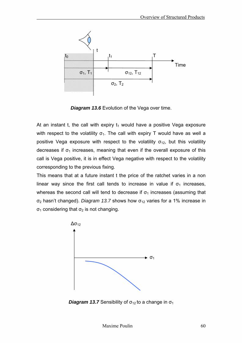
Overview of Structured Products
Maxime Poulin 60
Diagram 13.6 Evolution of the Vega over time.
At an instant t, the call with expiry t1 would have a positive Vega exposure
with respect to the volatility σ1. The call with expiry T would have as well a
positive Vega exposure with respect to the volatility σ12, but this volatility
decreases if σ1 increases, meaning that even if the overall exposure of this
call is Vega positive, it is in effect Vega negative with respect to the volatility
corresponding to the previous fixing.
This means that at a future instant t the price of the ratchet varies in a non
linear way since the first call tends to increase in value if σ1 increases,
whereas the second call will tend to decrease if σ1 increases (assuming that
σ2 hasn’t changed). Diagram 13.7 shows how σ12 varies for a 1% increase in
σ1 considering that σ2 is not changing.
Diagram 13.7 Sensibility of σ12 to a change in σ1
σ12, T12
σ2, T2
Time
t
σ1, T1
t0 t1 T
σ1
∆σ12
Overview of Structured Products
Maxime Poulin 61
It is easy to understand that the Vega is highly sensitive to the evolution of the
volatility term structure: change in the volatility of the volatility have therefore
to be taken into account.
It is important to highlight that in the case of a volatility surface moving all by
the same amount, the Vega would have shown a linear behavior.
13.2.3. Reverse Cliquet
A reverse cliquet can be generally defined as a globally floored option where
the payoff depends on locally capped performances. Usually a reverse cliquet
has a maximum payout starting at X which decreases as the sum of forward
starting put options increases in value. The payoff would therefore be:
⎟⎟⎠
⎞⎜⎜⎝
⎛⎟⎟⎠
⎞⎜⎜⎝
⎛−+= ∑
= −
N
i i
i
SS
MinXMaxPayoff1 1
1,0,0
The reverse cliquet is sensitive to both the volatility of volatility and the
forward skew. In the following section we will show why this is the case.
Reverse cliquet behavior
Let’s consider how the Vega of the reverse cliquet behaves when the volatility
varies from small to significant values. If the volatility is low, the sum of the
values of the ATM put options will be very sensitive in volatility changes since
a small shift in the surface will be reflected in the change in value of all the
single put options and the total Vega will therefore be the same as the sum of
the individual Vegas. If volatility is high, on the other hand, a small change in
the volatility surface will not affect the Vega since the probability for the puts
to be in the money is very high, which in turn is very likely to quickly exceed X.
The Vega profile can therefore be represented as follows:

Overview of Structured Products
Maxime Poulin 62
Diagram 13.8 Vega profile with respect to the volatility
The reverse cliquet, like several other similar cliquets, can therefore be
considered as a put option on volatility as shown in Diagram 13.9.
Diagram 13.9 Parallel between a put option and the Vega Profile
As we know a put option has a positive sensitivity to Vega. It is, therefore,
easy to see that if we are using a model which doesn’t take into account the
volatility of volatility we are in fact pricing a put option without its time value
and the price is therefore incorrect. A model which simulates the stochastic
behavior of volatility is here needed in order to correctly price the additional
feature.
Sigma
Vega
Sigma
Vega

Overview of Structured Products
Maxime Poulin 63
The reverse cliquet is equally sensitive to forward skew, even if its sensitivity
is here less important if compared to that of volatility of volatility. To see why
this is the case, we’ll analyze what the skew exposure is when we fix the last
strike (meaning the final fixing before maturity) at time t*.
Diagram 13.10 Final fixings of a Reverse Cliquet with maturity N
Let’s suppose that the following relation is valid at time t*
∑−
= −⎟⎟⎠
⎞⎜⎜⎝
⎛−+=′
1
1 1
1,0N
i i
i
SS
MinXX
The payoff at time t* for the maturity T is therefore:
⎟⎟⎠
⎞⎜⎜⎝
⎛⎟⎟⎠
⎞⎜⎜⎝
⎛−+′=
−
1,0,01N
N
SS
MinXMaxPayoff
This can be seen as being short an ATM call and long a call strike done by 1-
X’, both fixing the strike at N-1 and with expiry at N, as shown in Diagram
13.10.
t0
Time
N-1 N

Overview of Structured Products
Maxime Poulin 64
Diagram 13.11 Payoff a reverse cliquet (investor’s point of view)
The dotted line shows the total position of the holder of the reverse cliquet at
time t*, which results in a call spread. It is easy to see that the call one is long
is always in-the-money and this results in a positive sensitivity to skew for this
call. The call one is short, on the other hand, is always at-the-money and is
consequently non sensitive to skew. The total exposure is therefore a positive
exposure to skew.
13.2.4. Napoleon Cliquet
Let’s now consider a Napoleon with monthly resets, which pays a yearly
coupon expressed by the following formula:
⎟⎟⎠
⎞⎜⎜⎝
⎛⎟⎟⎠
⎞⎜⎜⎝
⎛−+=
−
1,01i
i
i SS
MinXMaxPayoff
Payoff
1-X’ S 1
Overview of Structured Products
Maxime Poulin 65
The client receives, therefore, a coupon of X plus an amount which
corresponds to the smallest monthly return. The Napoleon as well, like the
reverse cliquet, is sensitive to volatility of volatility and to forward skew.
Napoleon behavior
The Vega is, in this case again, a non-linear function of volatility. Let’s
consider the case where the volatility of volatility is close to zero. This means
that the volatility won't vary significantly from a given fixed value. The
individual monthly puts will therefore have a given probability to be in the
money and the more valuable of them will have a given probability Π1 to
assume a value X1. If we increase now the volatility of volatility the probability
associated to each monthly put will in general be different and the more
valuable of them will have a probability Π2 to assume the same a value X,
which will be greater than Π1. In other words, if we consider stochastic
volatility the most valuable monthly put will assume higher values compared
to the case where there is no volatility of volatility. If volatility is very high,
small shifts of the volatility surface will in general leave unaffected the price of
the Napoleon. Increasing the probability Π for the put being in the money will
have no effect on the price since the payoff has an overall floor at zero. The
Vega is therefore close to zero. This is not the case if volatility is low. In this
case increasing the probability Π will have a significant impact on the options
price and this corresponds to a significant Vega.
The Vega profile as a function of volatility is here again similar to the one
shown in Diagram 13.8.
Let’s now analyze the sensitivity of the Napoleon with respect to the forward
skew. The forward skew has less significant impact if compared to the reverse
cliquet. To understand this let’s see what the payoff would be at the last strike
date (the one before maturity):
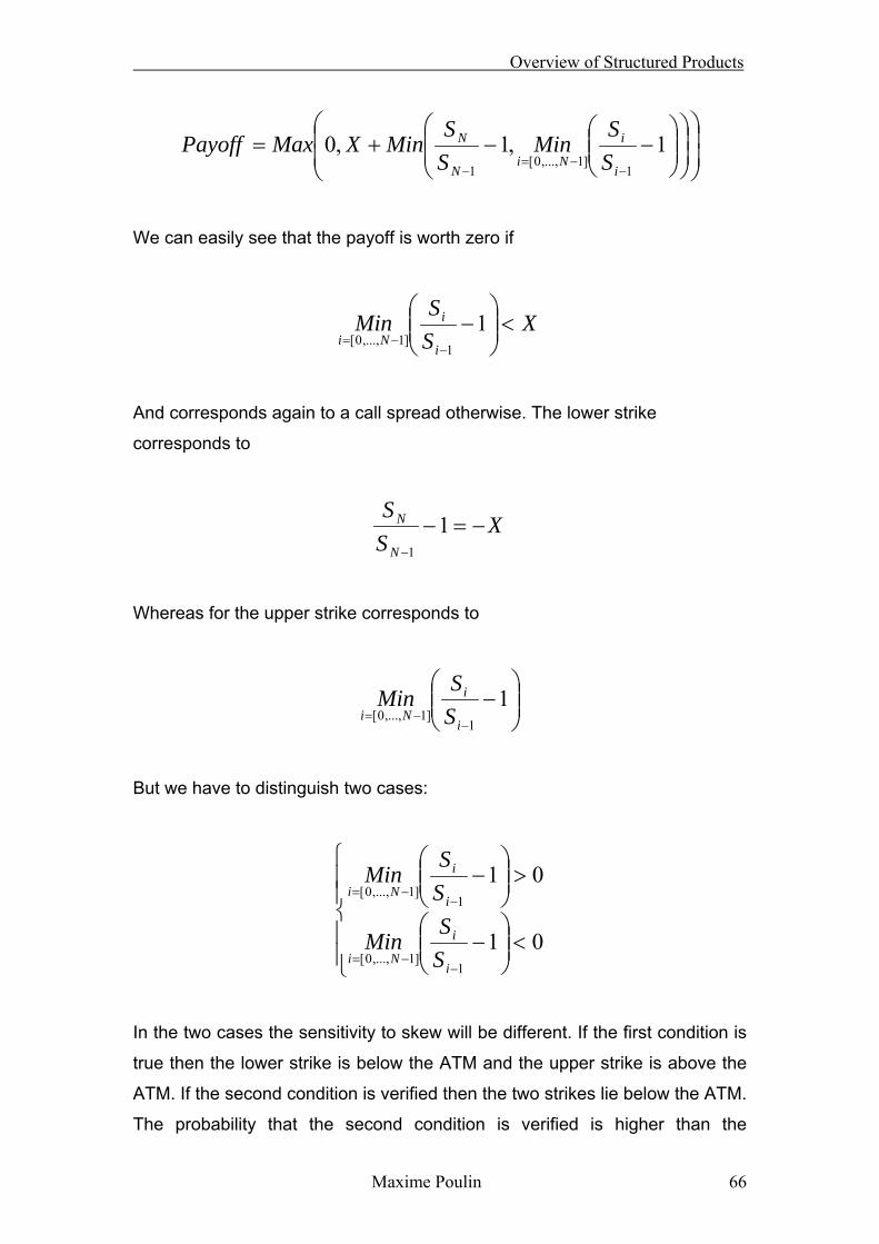
Overview of Structured Products
Maxime Poulin 66
⎟⎟⎠
⎞⎜⎜⎝
⎛⎟⎟⎠
⎞⎜⎜⎝
⎛⎟⎟⎠
⎞⎜⎜⎝
⎛−−+=
−−=
−
1,1,01
]1,...,0[1 i
i
NiN
N
SS
MinSS
MinXMaxPayoff
We can easily see that the payoff is worth zero if
XSS
Mini
i
Ni<⎟⎟
⎠
⎞⎜⎜⎝
⎛−
−−=
11
]1,...,0[
And corresponds again to a call spread otherwise. The lower strike
corresponds to
XSS
N
N −=−−
11
Whereas for the upper strike corresponds to
⎟⎟⎠
⎞⎜⎜⎝
⎛−
−−=
11
]1,...,0[i
i
Ni SS
Min
But we have to distinguish two cases:
⎪⎪⎩
⎪⎪⎨
⎧
<⎟⎟⎠
⎞⎜⎜⎝
⎛−
>⎟⎟⎠
⎞⎜⎜⎝
⎛−
−−=
−−=
01
01
1]1,...,0[
1]1,...,0[
i
i
Ni
i
i
Ni
SS
Min
SS
Min
In the two cases the sensitivity to skew will be different. If the first condition is
true then the lower strike is below the ATM and the upper strike is above the
ATM. If the second condition is verified then the two strikes lie below the ATM.
The probability that the second condition is verified is higher than the

Overview of Structured Products
Maxime Poulin 67
probability associated to the first condition. This is true since we are taking the
smallest return over the period. The two strikes tend, therefore, to be closer if
compared to the reverse cliquet. Since the holder of the option is long the call
spread he is effectively buying the call with the lower strike and selling the call
with higher strike. The contract is in general long skew where the overall
sensitivity is lower than the one of the reverse cliquet since the two strikes lie
closer in this case.

Overview of Structured Products
Maxime Poulin 68
Conclusion In this paper, we’ve seen the equity derivatives business model of banks
(especially Commerzbank’s equity derivatives business model), for whom
selling structured product has 2 main points of importance, being able to give
a fair price to these options, and being able to hedge away the risk brought
aboard by these options.
We’ve seen the way structured products are manufactured, and distributed,
as well as how these products are hedged on the trading side. We’ve also
explained the rationale behind the use of one financial model rather than
another one while pricing a specific option, the choice being driven by having
a model which takes into account the parameters which affected the
distribution of returns of this option.
Once the derivative has been priced, the structured product sold, the
responsibility is transferred to the traders who have the task to hedge away
the risk of these products (as we have seen, this is the Delta risk, Vega risk
and Correlation risk) by doing so on a daily basis, they incur either profits or a
losses depending on how accurate their pricing was, regardless of how the
market behaved.
At last we’ve taken the example of cliquets, an exotic structured product, on
which the pricing due to the second order risk is fairly complex, and on which
we’ve outlined the particularities of the payoff and the hedging specificities.
Overview of Structured Products
Maxime Poulin 69
Bibliography
[1] Allen, S. and Padovani, O., 2002. Risk Management Using Quasi-Static
Hedging. Econ. Notes 31(2)
[2] Avellaneda, M., Lévy, A. and Paras, A., 1995. Pricing and Hedging
Derivative Securities in Markets with Uncertain Volatilities. Appl. Math.
Finance 2,
[3] Carr, P., Geman, H. and Madan, D. B., 2001. Pricing and Hedging in
Incomplete Markets. J. Financ. Econ. 62
[4] Eraker, B., Johannes, M. and Polson, N., 2003. The impact of jumps in
volatility and returns. Journal of Finance, 58
[5] Fleming, J., Ostdiek, B. and Whaley, R. E., 1996. Trading costs and the
relative rates of price discovery in the stock, futures, and option markets.
Journal of Futures Markets, 16
[6] Hull, J. C., 2003. Options, Futures and Other Derivatives. 5th ed. Upper
Saddle River, New Jersey, U.S.A.: Prentice Hall.
[7] Maheu, J. M. and McCurdy, T. H., 2004. News arrival, jumps dynamics,
and volatility components for individual stock returns. Journal of Finance, 59
[8] Wilmott, P., 2007. Paul Wilmott introduces Quantitative Finance, 2nd ed.
Southern Gate, Chichester, West Sussex, England: The Atrium.
[9] Gudbrand and Koekebakker, Steen, Volatility and Price Jumps in
Agricultural Futures Prices - Evidence from Wheat Options. American Journal
of Agricultural Economics, Vol. 86, No. 4, pp. 1018-1031, November 2004.
Available at SSRN: http://ssrn.com/abstract=595052