○E

Surface Microseismic Monitoring of HydraulicFracturing of a Shale-Gas Reservoir UsingShort-Period and Broadband Seismic Sensorsby Xiangfang Zeng, Haijiang Zhang, Xin Zhang, Hua Wang,Yingsheng Zhang, and Qiang Liu

Online Material: Figure, table with double-difference eventlocations.

INTRODUCTION

Hydraulic fracturing has been widely applied in developmentof tight sand and shale gas reservoirs, in which high-pressurefluids are injected into target zones to enhance the reservoirpermeability so that gas can be more efficiently recovered. Theopening and growing of tensile fractures, as well as shearing slipalong fractures during stimulation treatment are thought to bethe major mechanisms inducing microseismic events around thetreatment well (Shemeta and Anderson, 2010). Therefore, mi-croseismic monitoring is a valuable approach to assess the frac-turing process. For example, the locations of microseismic eventsare used to determine fracture network geometry, and their focalmechanisms are helpful for understanding how the fractures arestimulated. The information derived from microseismic moni-toring is helpful for reservoir simulation and assessment (e.g.,Rutledge and Phillips, 2003; Warpinski, 2009; Maxwell, 2010).

However, injecting fluids into underground formations,especially wastewater disposal into deep wells, has caused feltor damaging earthquakes with magnitudes larger than 4 insome cases (Ellsworth, 2013). The well-documented cases in-clude Rocky Mountain Arsenal in the 1960s (Healy et al.,1968), wastewater disposal in Texas (Frohlich et al., 2011),Oklahoma (Holland, 2013), and Arkansas (Horton, 2012).In fact, an anomalous increase in earthquake activity has oc-curred in the central and eastern United States over the pastfew years, which is mainly due to deep injection of low-pressurewastewater into deep strata or basement formations (Ellsworth,2013). Hydraulic fracturing using high-pressure fluids can in-duce a lot of earthquakes, but the vast majority have magni-tudes smaller than 1 (Ellsworth, 2013). In some cases,hydraulic fracturing of shale gas can indeed cause relativelylarge and felt earthquakes, including anM 2.3 earthquake nearBlackpool, United Kingdom (Green and Styles, 2012), anM 4.0 earthquake near Youngstown, Ohio (Kim, 2013),

and an M 3.6 earthquake in the Horn River basin of BritishColumbia (BC Oil and Gas Commission, 2012).

The mechanism causing the induced seismicity is likely thewell-understood process of weakening a pre-existing fault/frac-ture by elevating the fluid pressure (Ellsworth, 2013). This isbecause by injecting fluids, pore pressure in connected poresand pre-existing faults/fractures also increases. If the tectonicstress of the underground formation is close to the criticalstress, it will lead to shear slip on pre-existing faults/fracturesand may cause large earthquakes. For this reason, microseismicmonitoring in real time is necessary for assessing the inducedseismic activity so that some measures could be taken to avoidinducing large-magnitude earthquakes (Majer et al., 2012).

In this study, we report results from a surface microseismicmonitoring of a multiple-stage hydraulic fracturing of a shalegas reservoir along a horizontal well in early 2013. The studyregion is located in southwest China, where many pilot wellshave been drilled to assess the shale gas development potentialin China (Fig. 1). For the target hydraulic fracturing shale layer,it has a small dip angle of 7° with a thickness of ∼300 m. Tofollow the strata trend, the horizontal well also has a dip angleof ∼7°. There are 21 fracturing stages along the 1400 m-longhorizontal well. The actual depth intervals of hydraulic frac-turing range from ∼2700 to ∼3000 m (shadowed zone inFig. 1a) from heel to toe. According to the well-logging data,limestone is the main rock type for the segment above 1300 m,whereas mudstone is the major rock type below 1300 m. Thetarget layer is composed of shale and clay. Acoustic logging dataprovides a P-wave velocity profile between 1100 and 2400 m.The low-velocity layer corresponds to mudstone, whereas thehigh-velocity layer corresponds to the limestone (Fig. 1a).

Currently, for microseismic monitoring of hydraulic frac-turing in industry, generally either downhole or surface mon-itoring is selected. For downhole microseismic monitoring,single or multiple strings of high-frequency (e.g., 15 Hz) geo-phones are installed in nearby well(s) (Warpinski et al., 2012).For surface microseismic monitoring, densely spaced geo-phones consisting of thousands of high-frequency and

668 Seismological Research Letters Volume 85, Number 3 May/June 2014 doi: 10.1785/0220130197

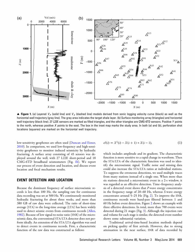
low-sensitivity geophones are often used (Duncan and Eisner,2010). In comparison, we used low-frequency and high-sensi-tivity geophones to monitor induced seismicity by hydraulicfracturing. A surface array consisting of 45 sensors was de-ployed around the well, with 27 L22E short-period and 18CMG-6TD broadband seismometers (Fig. 1b). We reportour process of event detection and location, and discuss eventlocation and focal mechanism results.

EVENT DETECTION AND LOCATION

Because the dominant frequency of surface microseismic re-cords is less than 100 Hz, the sampling rate for continuousdata recording was set at 500 Hz. We continuously monitoredhydraulic fracturing for about three weeks, and more than380 GB of raw data were collected. The ratio of short-timeaverage (STA) to the long-time average (LTA) has been widelyused to detect seismic events from continuous records (Allen,1982). Because of low signal-to-noise ratio (SNR) of the micro-seismic data, the conventional STA/LTA detector does not per-form ideally. An extension of the STA/LTA algorithm was usedto detect events in continuous records. First, a characteristicfunction of the raw data was constructed as follows

cf�i� � X 2�i� − X�i� 1� × X�i − 1�; �1�

which includes amplitude and its gradient. The characteristicfunction is more sensitive to a rapid change in waveform. Thenthe STA/LTA of the characteristic function was used to iden-tify the microseismic signal. Traffic noise and missing datacould also increase the STA/LTA ratios at individual stations.To suppress the erroneous detections, we used multiple tracesfrom many stations instead of a single one. When more thansix stations detected a microseismic event in a 2-s window, itwas regarded as an effective detection. Time–frequency analy-sis of a detected event shows that P-wave energy concentratesin the frequency range of 20–60 Hz, whereas S-wave energyconcentrates around 5–25 Hz (Fig. 2). To improve the SNR,continuous records were band-pass filtered between 1 and60 Hz before event detection. Figure 2 shows an example withthree effective detections. In total, more than 700 events weredetected during 21 stages (Fig. 3). Although the injection rateand volume for each stage is similar, the detected event numbershows some substantial variation.

Traditional arrival-time-based location methods dependon picking quality of first arrivals. However, due to strongattenuation in the near surface, SNR of data recorded by

Y (

m)

(a) (b)

X (m)

Z (

m)

Vel (m/s)

X (m)

limestone

mudstone

shale & clay

−2000

−1500

−1000

−500

0

500

1000

1500

−2000 −1500 −1000 −500 0 500 1000 1500

X12

X13

X14

X15

X21

X22

X25X26

X31

X32

X33

X34

X35X36

X41

X42X43

X44

X45

X46

X47

X51

X52X53

X54

X55X56

X61X62X63

X64X65

X66

X73

X74X75

X76

X80X85

X91X92

80° 100° 120°20°

30°

40°

50°0

1000

2000

3000

0 2000 4000 6000

1000

2000

3000

1000

2000

3000

▴ Figure 1. (a) Layered V P (solid line) and V S (dashed line) models derived from sonic logging velocity curve (black) as well as thehorizontal well trajectory (gray line). The gray area indicates the target shale layer. (b) Surface monitoring array (triangles) and horizontalwell trajectory (black line). 27 L22E sensors are marked as filled triangles, and the other triangles are CMG-6TD sensors. Positive Y pointsto the north, whereas positive X points to the east. The box in the inset map marks the study area. In both (a) and (b), perforation shotlocations (squares) are marked on the horizontal well trajectory.

Seismological Research Letters Volume 85, Number 3 May/June 2014 669

surface monitoring array is usually lower than that of boreholemicroseismic data. Low SNR of surface monitoring data gen-erally leads to high-picking errors by an automatic picker or ananalyst, thus resulting in large event location uncertainty. Insome cases, it is even impossible to determine first arrivals fromnoisy records. In comparison, a migration-based locationmethod does not need first arrival picking and has been suc-cessfully applied to locate glacial earthquakes, tremors, and

noise sources (Ekström et al., 2003; Kao and Shan, 2004; Zengand Ni, 2010). For the migration-based location method, wediscretized the region into 3D grid nodes. Each node can bepotentially regarded as a microseismic source. The records arestacked according to travel times between stations and hypo-thetic source location, as well as the assumed origin time. Theoptimal origin time and event location are found when thestacking energy is maximum. Because of the uncertainty inthe velocity model for calculating travel times and differentradiation patterns at different stations, the waveforms couldbe out of phase, and thus direct stacking of original recordscould cancel each other out. Therefore, we stacked waveformenvelopes instead of raw waveforms. The objective function isdefined as

OBJ�x; y; z; τ� �XN

i�1

Xt0

t�−t0

fwi�Ti�x; y; z� � τ� t�g: �2�

In the above equation, x, y, z, and τ are possible eventcoordinates in a 3D grid and origin time, Ti�x; y; z� is the traveltime from the grid point of �x; y; z� to receiver, t0 is the half-time window size for stacking, wi is the normalized waveformenvelope at the receiver, and N is the number of receivers.

A finite-difference travel-time calculation method basedon the eikonal equation was employed to calculate travel timesbetween stations and search grid nodes (Podvin and Lecomte,1991). During the grid-search procedure, travel time is readfrom the travel-time table saved on disk to speed the search

41120 41160 41200

X13

X36

X51

X56

X85

X91

X13_sta_lta

X36_sta_lta

0 20 40 60 80

Time (sec)

Frequency (Hz)

13-60-40-20

0204060

X36 002JAN 20 (020), 201300:00:00.000

41102 41104 41106 41108 41110 41112 41114

0

5

10

41104 41106 41108 41110 41112 411140

20

40

60

80

100

(a)

(c)

(d)

41102 41104 41106 41108 41110 41112 41114

-4

-2

0

2

4

X 10-7

X36 002JAN 20 (020), 201300:00:00.000 4

2 0–2–4

(b)

41104 41108 4111210×10-7 m/s

▴ Figure 2. (a) Traces recorded on six stations as well as theshort-time average (STA)/long-time average (LTA) ratios of the cor-responding characteristic functions on stations X36 and X13.(b) Trace consisting of a detected event recorded at stationX36 (box in panel a). (c) Spectrogram of the waveform data inpanel b. And (d), frequency spectrum of the waveform in panel b.

0

500

1000

1500

2000

2500

0 5 10 15 20

0

30

60

90

0 5 10 15 20

Inje

ctio

n V

olum

e (m

3)E

vent

Num

ber

Stage

▴ Figure 3. The injection fluid volume (upper panel) and the de-tected microseismic event number (lower panel) at each stage.The fluid volume data are not available after stage 14.

670 Seismological Research Letters Volume 85, Number 3 May/June 2014

process. From the waveform of the detected event, it can beseen that the S wave is much stronger than the P wave, similarto other studies (Fig. 2). For this reason, we only stackedenvelopes of the filtered seismograms in the S-wave windows.Because the S wave is stronger on horizontal components, weonly stacked the north components. For stacking, a P-wavevelocity profile between depth 1100 and 2400 m was obtainedfrom well sonic logging (Fig. 1a). We construct a layeredS-wave velocity model with different VP=V S ratios accordingto the rock type (Fig. 1a). The VP=V S ratios were chosen as1.89 for limestone and 2.2 for shale (Castagna et al., 1985).

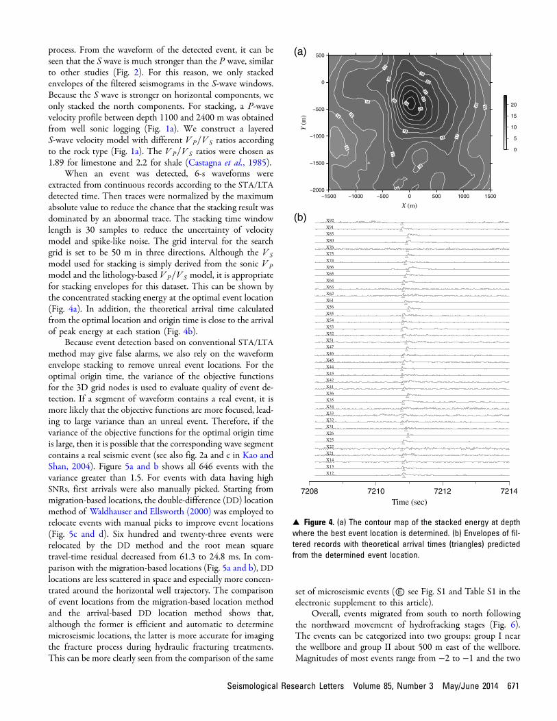
When an event was detected, 6-s waveforms wereextracted from continuous records according to the STA/LTAdetected time. Then traces were normalized by the maximumabsolute value to reduce the chance that the stacking result wasdominated by an abnormal trace. The stacking time windowlength is 30 samples to reduce the uncertainty of velocitymodel and spike-like noise. The grid interval for the searchgrid is set to be 50 m in three directions. Although the V Smodel used for stacking is simply derived from the sonic VPmodel and the lithology-based VP=V S model, it is appropriatefor stacking envelopes for this dataset. This can be shown bythe concentrated stacking energy at the optimal event location(Fig. 4a). In addition, the theoretical arrival time calculatedfrom the optimal location and origin time is close to the arrivalof peak energy at each station (Fig. 4b).

Because event detection based on conventional STA/LTAmethod may give false alarms, we also rely on the waveformenvelope stacking to remove unreal event locations. For theoptimal origin time, the variance of the objective functionsfor the 3D grid nodes is used to evaluate quality of event de-tection. If a segment of waveform contains a real event, it ismore likely that the objective functions are more focused, lead-ing to large variance than an unreal event. Therefore, if thevariance of the objective functions for the optimal origin timeis large, then it is possible that the corresponding wave segmentcontains a real seismic event (see also fig. 2a and c in Kao andShan, 2004). Figure 5a and b shows all 646 events with thevariance greater than 1.5. For events with data having highSNRs, first arrivals were also manually picked. Starting frommigration-based locations, the double-difference (DD) locationmethod of Waldhauser and Ellsworth (2000) was employed torelocate events with manual picks to improve event locations(Fig. 5c and d). Six hundred and twenty-three events wererelocated by the DD method and the root mean squaretravel-time residual decreased from 61.3 to 24.8 ms. In com-parison with the migration-based locations (Fig. 5a and b), DDlocations are less scattered in space and especially more concen-trated around the horizontal well trajectory. The comparisonof event locations from the migration-based location methodand the arrival-based DD location method shows that,although the former is efficient and automatic to determinemicroseismic locations, the latter is more accurate for imagingthe fracture process during hydraulic fracturing treatments.This can be more clearly seen from the comparison of the same

set of microseismic events (Ⓔ see Fig. S1 and Table S1 in theelectronic supplement to this article).

Overall, events migrated from south to north followingthe northward movement of hydrofracking stages (Fig. 6).The events can be categorized into two groups: group I nearthe wellbore and group II about 500 m east of the wellbore.Magnitudes of most events range from −2 to −1 and the two

7208 7210 7212 7214

X12

X13

X14

X21

X22

X25

X26

X31

X32

X33

X34

X35

X36

X41

X42

X43

X44

X45

X46

X47

X51

X52

X53

X54

X55

X56

X61

X62

X63

X64

X65

X66

X74

X75

X76

X80

X85

X91

X92

Time (sec)

−2000

−1500

−1000

−500

0

500

13

14

15

15

16

16

16

16

17

17

17

18

18

19

19

20

20

2122

23

24

−1500 −1000 −500 0 500 1000 1500

0

5

10

15

20

X (m)

Y (

m)

(a)

(b)

▴ Figure 4. (a) The contour map of the stacked energy at depthwhere the best event location is determined. (b) Envelopes of fil-tered records with theoretical arrival times (triangles) predictedfrom the determined event location.

Seismological Research Letters Volume 85, Number 3 May/June 2014 671

groups have similar distributions (Fig. 7). The b-value for thedetected microseismic events is about 1.0. During the first ninestages, events mostly occurred near the wellbore and perfora-tion locations. However, starting from stage one, events alsooccur far away from the wellbore and in the group II (Fig. 6a).For the first nine stages, the group II events generally follow thenortheast–southwest trend of ∼60° (dashed line in Fig. 6a). Atstage 10, a cluster of events is located to the east of the wellboreand is nearly perpendicular to the wellbore (dashed line inFig. 6c). This cluster of events starts to form the majorityof events of group II and until stage 16, many events repeatedlyoccur in the same area. After stage 16, there are fewer eventsdetected and located. Although stimulation parameters for dif-ferent stages are similar, earlier and later stages induce muchfewer events than stages 10–16. It can also be seen that the

group II events show two major strikes, 60° and 90°(Fig. 6a,c).

FOCAL MECHANISM ANALYSIS

The location distribution of induced events is helpful to under-stand stimulated reservoir volume and fracture geometry. Thefocal mechanisms of induced events provide additional infor-mation about fractures. Furthermore, we can use focal mech-anisms to derive local stress directions. Several methods havebeen proposed to invert for focal mechanisms of microseismicevents using first-motion polarities, relative amplitudes of firstarrivals or even full waveforms (Zoback and Harjes, 1997;Duncan and Eisner, 2010; Li et al., 2011). Most of small in-duced microseismic events could be approximated by a double-couple point source (Rutledge and Phillips, 2003) and P wave

–1500

–1000

–500

0

500

1000

–1500 –1000 –500 0 500 1000 1500

0

4

8

12

16

20

1000

1500

2000

2500

3000

3500–1500 –1000 –500 0 500 1000

Y (m)X (m)

Y (

m)

Z (

m)

Y (

m)

Z (

m)

Y (m)X (m)

0

4

8

12

16

20

–1500

–1000

–500

0

500

1000

–1500 –1000 –500 0 500 1000 1500

0

4

8

12

16

20

1000

1500

2000

2500

3000

3500–1500 –1000 –500 0 500 1000

0

4

8

12

16

20

III

(b)(a)

(d)(c)

▴ Figure 5. (a) Map view of migration-based event locations; (b) east side view of migration-based event locations; (c) map view of DDevent locations; and (d) east side view of double-difference (DD) event locations. The two boxes on panel (c) indicate event group I and II,respectively. Dot colors denote different stages.

672 Seismological Research Letters Volume 85, Number 3 May/June 2014

(b)(a)

(d)(c)

(f)(e)

Y (

m)

X (m) X (m)

Y (

m)

Y (

m)

X (m) X (m)

Y (

m)

Y (

m)

X (m) X (m)

Y (

m)

–1500

–1000

–500

0

500

1000

–1500 –1000 –500 0 500 1000 1500

stage1stage2stage3

–1500

–1000

–500

0

500

1000

–1500 –1000 –500 0 500 1000 1500

stage4stage5stage6stage7

–1500

–1000

–500

0

500

1000

stage8stage9stage10

–1500

–1000

–500

0

500

1000

stage11stage12stage13

–1500

–1000

–500

0

500

1000

–1500 –1000 –500 0 500 1000 1500

–1500 –1000 –500 0 500 1000 1500

stage14stage15stage16

–1500

–1000

–500

0

500

1000

–1500 –1000 –500 0 500 1000 1500

–1500 –1000 –500 0 500 1000 1500

stage17stage18stage19stage20stage21

▴ Figure 6. Map view of event locations for different stages of hydraulic fracturing. (a) Stages 1–3; (b) stages 4–7; (c) stages 8–10;(d) stages 11–13; (e) stages 14–16; and (f) stages 17–21. Dashed lines delineate the faults/fractures illuminated by induced events.

Seismological Research Letters Volume 85, Number 3 May/June 2014 673

first-motion polarities have been widely used to determine thefault plane of the double-couple source. The polarity is con-trolled by fault plane and take-off vector. In this study, we em-ployed the HASH method developed by Hardebeck andShearer (2002) to determine event focal mechanisms. Thetake-off vector is derived from ray-path azimuth and incidenceangle that are obtained from ray tracing in a layered velocitymodel. P wave first-motion polarities were manually picked onvertical records.

In total, we obtained focal mechanisms of 154 events withat least eight picks (Fig. 8a). Because of the uncertainty in theVP model and the coverage gap of the available stations withclear first-motion polarities, it is expected that the obtainedfocal mechanisms also have some uncertainties. We used themisfit of the first-motion polarities to measure the focal mecha-nism solution quality (Hardebeck and Shearer, 2002). Theaverage weighted misfit of first-motion polarities is less than30.7% (Ⓔ see Table S2 in the electronic supplement). Toquantitatively describe the distribution of focal mechanisms,we projected them into a triangle diagram according to theprincipal axes (Frohlich and Apperson, 1992). The triangle di-agram is helpful to recognize event orientation clusters. For theanalyzed events, the distribution of focal mechanisms is almostuniform over the focal projection. Figure 8b shows the trianglediagram for different groups of selected events, which suggeststhere are no significant differences between the two groups.The azimuths of compressive P axes are shown in a polar histo-gram (Fig. 8c). Most P-axis azimuths fall into the northwest tonorth-northeast directions, which is consistent with the

regional-tectonic stress direction. Because of the ambiguityof the fault plane, it is difficult to determine the rupture plane.Therefore, both fault and conjugate fault are adopted in thestatistics. There are two peaks (north-northeast and east-north-east) in the polar histogram (Fig. 8d). This is consistent withthe previous geological survey, in which the orientation of frac-tures was found to range from 30° to 70° (H. Liu, personalcomm., 2013). The active seismic survey also reveals an existingnortheast–southwest fault in the region (H. Liu, personalcomm.). Combining with the location results, it suggests thatmost induced events likely occurred on natural fractures.

DISCUSSION

Earthquakes release stored elastic strain energy when a shear ortensile failure occurs on a fault. The Coulomb failure condi-tion is controlled by friction coefficient, normal stress, andpore pressure (Hubbert and Rubey, 1959). The earthquakescould be induced by increasing the shear stress, decreasingthe normal stress, and/or elevating the pore pressure. Whenpore pressure exceeds the sum of the least principal stressand the tensile strength of the rock, it will fail in tension. Be-cause the effective normal stress decreases as pore pressure in-creases, the shear failure occurs before pore pressure exceeds σ3.In active tectonic regions, the rock is very likely critically

00

2020

4040

6060

8080

100100

–3 −2 −1 0

Magnitude

▴ Figure 7. Histograms of magnitudes for group I (filled) andgroup II (unfilled) events.

Y (

m)

X (m)Strike Slip

tsurhTlamroN

(a)

(c)(b) (d)

I

II

–1500

–1000

–500

0

500

1000

–1500 –1000 –500 0 500 1000 1500

10

E

N

10

E

N

▴ Figure 8. (a) Map view of focal mechanisms; (b) triangle dia-gram of focal mechanisms, circle and cross denote events fromgroup I and II, respectively.; (c) distribution of azimuths of P axes;and (d) distribution of azimuths of fault-plane strikes.

674 Seismological Research Letters Volume 85, Number 3 May/June 2014

stressed (Zoback and Harjes, 1997), and small shear-stress/pore-pressure perturbation will cause fault slip. The earth-quakes could be induced at the source of or away fromstress/pore-pressure change (Ellsworth, 2013). The propaga-tion of pore-stress perturbation is complex. In saturated rockswith low permeability, linear relaxation of pore-pressure per-turbation plays a dominant role, whereas infiltration of fluidcontrols propagation rate (Shapiro and Dinske, 2009). Exten-sion of fracture networks also leads to pore-pressure perturba-tion as well as the loss of fracturing fluid into surroundingrocks. The first mechanism shows a linear diffusion rate duringfluid injection, whereas the latter mechanism shows a morecomplex pattern (e.g., Shapiro et al., 2006). In the Perkins–Kern–Nordgren (PKN) model, both mechanisms of pore stressperturbation propagation suggest expansion of the trigger frontis approximately proportional to the square root of time (Sha-piro et al., 2006). In comparison, for the Christianovitch–Geertsma–De Klerk-Danesh (CGDD) model, it predicts theinduced events expand in proportion to 2=3 power of time(Mendelsohn, 1984), which is better than the PKN modelfor fitting the expansion of microseismicity with time inthe Hijiori site, Japan (Sasaki, 1998). However, because ofthe incompleteness of the microseismic events detected in thisdataset, it is difficult to show which model is more appropriate.

In this study, the group of events occurring along the well-bore seems consistent with the diffusion pattern and is near thesource of stress/pore-pressure perturbation. However, duringhydraulic fracturing stage 1, there are two events detectedand located about 1.5 km away from the perforation spot.These two events occurred about 4.5 and 7.5 hours afterthe start of fluid injection, respectively. The fluid could rapidlymove along a high-permeability fault, and thus the two earth-quakes may be induced by the pore-pressure increase directlycaused by fluid migrated from the fracturing spot. Similarly, inthe case of the Horn river basin, Canada, the earthquakes aretriggered along a pre-existing fault at about 200 m away fromthe wellbore within tens to thousands of minutes after injec-tion (BC Oil and Gas Commission, 2012). The short timedelay would require a high-permeability fault. Lockner et al.(2000) reported that the highest matrix permeability is upto 100 microdarcies in the damage zone of the Nojima faultof the 1995 Kobe earthquake. Indeed, the active seismic surveyalso reveals an existing northeast–southwest fault in the region(H. Liu, personal comm.). In this case, the transmission of porepressure is very fast to a significant distance and is likely tocause the two earthquakes in stage 1. Alternatively, the twoearthquakes could be caused by stress perturbation resultingfrom undrained response of fluid injection (Talwani et al.,2007). If the areas with earthquakes induced are in a criticalstress condition, a small stress perturbation could induce faultslip. In the following stages of 2 to 9, there are a few earth-quakes induced away from the wellbore, sparsely distributedwithin ∼1:5 km of the wellbore. These earthquakes are nomi-nally aligned in the direction of ∼60° from the north, indicat-ing they occur along the existing faults (Fig. 6a).

For stage 10, there are more earthquakes detected and lo-cated than previous stages. These earthquakes are aligned al-most perpendicular to the wellbore, and most of them arelocated to the northeast with respect to the perforation spot.If the wellbore is drilled along the horizontal minimal com-pressive stress direction, fracking-induced events would gener-ally align perpendicular to the wellbore. However, from thefocal mechanism analysis, the local horizontal maximum stressdirection is approximately northwest–southeast. Therefore,these microseismic events are not directly induced by fracking,but instead most likely by reactivation along pre-existing faults/fractures. In the following stages of 11–16, there are manyevents repeatedly induced in the same region of ∼500 to1000 m to the east of wellbore. It is likely that the fracturingstage 10 opened a fluid conduit to the seismicity-clusteringzone that is critically stressed and highly fractured. In the laterstages of 11–16, the fluid can directly migrate to the clusteringzone, increasing pore pressure and inducing many earthquakes.

Pre-existing faults may provide a direct conduit of fluid,which may cause a long distance trigger (Ake et al., 2005; Hor-ton, 2012). The permeability of shale is about 0.1 microdarcy,whereas the permeability of fault zone is about two orders ofmagnitude higher (Best and Katsube, 1995; Evans et al., 1997).The breaking and crushing of grains during tectonic activitiescould create a fault-damage zone, which contains a mass ofcracks. High-crack density increases the pore volume and fluidtransport capability, for example, up to 100 microdarcies(Lockner et al., 2000). The migrated fluid reduced the effectivenormal pressure that leads to slip of the fault. If the fault hasbeen critically stressed and has lower friction coefficient, asmall increase of pore pressure can result in a higher triggeringprobability, such as the case of the increased microseismic ac-tivity after stage 10. It is noted that the number of detectedevents shows an obvious decrease after stage 17. This couldbe due to less fluid leaking from the horizontal well to thepre-existing fracture/fault zone, because the leak points of pres-sured fluids are located to the south of the bridge plug ofstage 17.

CONCLUSIONS

We used a broadband 3C seismic array installed on the surfaceto monitor microseismicity induced by 21 stages of hydraulicfracturing. Based on a migration-based location method andthe DD location method, we obtained locations of 665 events.Our study shows that with a relatively sparse surface array it isalso possible to detect and locate small magnitude events(M <−1) induced by hydraulic fracturing. Therefore, for mon-itoring hydraulic fracturing in some regions with favorable sur-face conditions and relatively shallow reservoir zones, it ispossible to use a sparse surface array.

The seismicity mainly forms two groups. Group I falls intoa small volume surrounding the horizontal well and group IIoccurs ∼500 m away from the well. We also determined focalmechanisms of 154 events with P wave first-motion polarities.The focal mechanism results show similar compressive stress

Seismological Research Letters Volume 85, Number 3 May/June 2014 675

axis strike (northwest–north-northeast) to the regional tec-tonic stress direction. Both two groups show similar patternsin the triangle diagram of focal mechanisms and the strikes offault planes are also consistent with previous geological survey.Based on locations and focal mechanisms, we conclude that thegroup I events are likely induced by the pore pressure increasedirectly caused by fluid migrated from the fracturing spot. Incomparison, the group II events are likely due to reactivation ofpre-existing faults/fractures by pressure perturbation fromfracking, which also provide a conduit for high-pressure fluidmovement.

Because the magnitude of microseismicity observed in thisstudy is small, the risk is low. Nevertheless, it is shown thatinjected fluids could leak to nearby pre-existing faults and trig-ger earthquakes. There are several reports that injection of flu-ids induced felt or even damaging earthquakes on pre-existingfaults (e.g., Horton, 2012; Kim, 2013). To reduce the risk ofinjection-induced earthquakes, better understanding of pre-existing faults, tectonic stress regime in the region, and appro-priate design and management of the injection program wouldbe necessary (Ellsworth, 2013).

ACKNOWLEDGMENTS

We are grateful to the editor Zhigang Peng, Clifford Thurber,and an anonymous reviewer for their comments that helped toimprove this paper. This research is supported by Natural Sci-ence Foundation of China under Grant Number 41274055and the Fundamental Research Funds for the Central Univer-sities (WK2080000053). This research is also partly supportedby the National Key Basic Research Program of China underGrant Number 2014CB845900.

REFERENCES

Ake, J., K. Mahrer, D. O’Connell, and L. Block (2005). Deep-injectionand closely monitored induced seismicity at Paradox Valley, Colo-rado, Bull. Seismol. Soc. Am. 95, no. 2, 664–683.

Allen, R. (1982). Automatic phase pickers: Their present use and futureprospects, Bull. Seismol. Soc. Am. 72, no. 6B, S225–S242.

Best, M. E., and T. J. Katsube (1995). Shale permeability and its signifi-cance in hydrocarbon exploration, TLE 14, no. 3, 165–170.

British Columbia (BC) Oil, and Gas Commission (2012). Investigation ofobserved seismicity in the Horn River Basin, Victoria, British Colum-bia, Canada, www.bcogc.ca/node/8046/download?documentID=1270(last accessed March 2014).

Castagna, J. P., M. L. Batzle, and R. L. Eastwood (1985). Relationshipsbetween compressional-wave and shear-wave velocities in clasticsilicate rocks, Geophysics 50, no. 4, 571–581.

Duncan, P., and L. Eisner (2010). Reservoir characterization using surfacemicroseismic monitoring, Geophysics 75, no. 5, 75A139–75A146.

Ekström, G., M. Nettles, and G. A. Abers (2003). Glacial earthquakes,Science 302, no. 5645, 622–624.

Ellsworth, W. L. (2013). Injection-induced earthquakes, Science 341,142 pp.

Evans, J. P., C. B. Forster, and J. V. Goddard (1997). Permeability of fault-related rocks, and implications for hydraulic structure of fault zones,J. Struct. Geol. 19, no. 11, 1393–1404.

Frohlich, C., and K. D. Apperson (1992). Earthquake focal mechanisms,moment tensors, and the consistency of seismic activity near plateboundaries, Tectonics 11, no. 2, 279–296.

Frohlich, C., C. Hayward, B. Stump, and E. Potter (2011). TheDallas–Fort worth earthquake sequence: October 2008 throughMay 2009, Bull. Seismol. Soc. Am. 101, no. 1, 327–340.

Green, C. A., and P. Styles (2012). Preese Hall shale gas fracturing:Review and recommendations for induced seismicity mitigation,www.gov.uk/government/uploads/system/uploads/attachment_data/file/15745/5075‑preese‑hall‑shale‑gas‑fracturing‑review.pdf (last ac-cessed March 2014).

Hardebeck, J. L., and P. M. Shearer (2002). A new method for determin-ing first-motion focal mechanisms, Bull. Seismol. Soc. Am. 92, no. 6,2264–2276.

Healy, J. H.,W. W. Rubey, D. T. Griggs, and C. B. Raleigh (1968). TheDenver earthquakes, Science 161, no. 3848, 1301–1310.

Holland, A. A. (2013). Earthquakes triggered by hydraulic fracturingin south-central Oklahoma, Bull. Seismol. Soc. Am. 103, no. 3,1784–1792.

Horton, S. (2012). Disposal of hydrofracking waste fluid by injectioninto subsurface aquifers triggers earthquake swarm in centralArkansas with potential for damaging earthquake, Seismol. Res. Lett.83, no. 2, 250–260.

Hubbert, M. K., and W. W. Rubey (1959). Role of fluid pressure in me-chanics of overthrust faulting I. Mechanics of fluid-filled porous sol-ids and its application to overthrust faulting,Geol. Soc. Am. Bull. 70,no. 2, 115–166.

Kao, H., and S. J. Shan (2004). The source-scanning algorithm: Mappingthe distribution of seismic sources in time and space, Geophys. J. Int.157, no. 2, 589–594.

Kim,W.-Y. (2013). Induced seismicity associated with fluid injection intoa deep well in Youngstown, Ohio, J. Geophys. Res. 118, 3506–3518,doi: 10.1002/jgrb.50247.

Li, J., H. Zhang, H. Sadi Kuleli, and M. Nafi Toksoz (2011). Focalmechanism determination using high-frequency waveform match-ing and its application to small magnitude induced earthquakes,Geophys. J. Int. 184, no. 3, 1261–1274.

Lockner, D., H. Naka, H. Tanaka, H. Ito, and R. Ikeda (2000).Permeability and strength of core samples from the Nojima fault ofthe 1995 Kobe earthquake, in H. Ito, K. Fujimoto, H. Tanaka, andD. Lockner (Editors), Proc. of the InternationalWorkshop on the NojimaFault Core and Borehole Data Analysis, Tsukuba, Japan, 22–23 Novem-ber 1999, U.S. Geol. Surv. Open-File Rept. 00-129, 147–152.

Majer, E. L., J. Nelson, A. Robertson-Tait, J. Savy, and I. Wong (2012).Protocol for addressing induced seismicity associated with enhancedgeothermal systems, DOE/EE‐0662, U.S. Department of Energy.

Maxwell, S. (2010). Microseismic: Growth born from success, TLE 29,no. 3, 338–343.

Mendelsohn, D. A. (1984). A review of hydraulic fracture modeling. I:General concepts, 2D models, motivation for 3D modeling,J. Energy Res. Technol. 106, no. 3, 369–376.

Podvin, P., and I. Lecomte (1991). Finite difference computation oftraveltimes in very contrasted velocity models: A massivelyparallel approach and its associated tools, Geophys. J. Int. 105,no. 1, 271–284.

Rutledge, J. T., and W. S. Phillips (2003). Hydraulic stimulation of natu-ral fractures as revealed by induced microearthquakes, CarthageCotton Valley gas field, east Texas, Geophysics 68, no. 2, 441–452.

Sasaki, S. (1998). Characteristics of microseismic events induced duringhydraulic fracturing experiments at the Hijiori hot dry rockgeothermal energy site, Yamagata, Japan, Tectonophysics 289,no. 1, 171–188.

Shapiro, S. A., and C. Dinske (2009). Fluid-induced seismicity: Pressurediffusion and hydraulic fracturing, Geophys. Prospect. 57, no. 2,301–310, doi: 10.1111/j.1365-2478.2008.00770.x.

Shapiro, S. A., C. Dinske, and E. Rothert (2006). Hydraulic-fracturingcontrolled dynamics of microseismic clouds, Geophys. Res. Lett. 33,no. 14, L14312, doi: 10.1029/2006GL026365.

Shemeta, J., and P. Anderson (2010). It’s a matter of size: Magnitude andmoment estimates for microseismic data, TLE 29, no. 3, 296–302.

676 Seismological Research Letters Volume 85, Number 3 May/June 2014

Talwani, P., L. Chen, and K. Gahalaut (2007). Seismogenic permeability,K s, J. Geophys. Res. 112, no. B07309, doi: 10.1029/2006JB004665.

Waldhauser, F., and W. L. Ellsworth (2000). A double-difference earth-quake location algorithm: Method and application to the northernHayward fault, California, Bull. Seismol. Soc. Am. 90, no. 6, 1353–1368.

Warpinski, N. (2009). Microseismic monitoring: Inside and out, J. Petrol.Technol. 61, no. 11, 80–85.

Warpinski, N. R., J. Du, and U. Zimmer (2012). Measurements of hy-draulic-fracture-induced seismicity in gas shales, SPE Prod. Oper.27, no. (3), 240–252.

Zeng, X., and S. Ni (2010). A persistent localized microseismic sourcenear the Kyushu Island, Japan, Geophys. Res. Lett. 37, no. 24,L24307, doi: 10.1029/2010GL045774.

Zoback, M. D., and H. P. Harjes (1997). Injection-induced earthquakesand crustal stress at 9 km depth at the KTB deep drilling site,Germany, J. Geophys. Res. 102, no. B8, 18477–18491.

Xiangfang Zeng1

Haijiang Zhang2

Xin Zhang2

Hua Wang3

Wantai-BMT Microseismic Lab ofSchool of Earth and Space Sciences

University of Science and Technology of ChinaHefei 230026, Chinazhang11@ustc.edu.cn

Yingsheng ZhangQiang Liu

Beijing Miseis TechnologiesBeijing 100096, China

1 CAS Key Laboratory of Computational Geodynamics, University ofChinese Academy of Sciences, Beijing 100049, China.2 Laboratory of Seismology and Earth’s Interior, University of Scienceand Technology of China, Hefei 230026, China.3 College of Geophysics and Information Engineering, Petroleum Uni-versity, Beijing 102249, China.

Seismological Research Letters Volume 85, Number 3 May/June 2014 677