
Dynamics of Bora wind over the Adriatic Sea: atmospheric ... · The Bora wind is a mesoscale...
150
Alma Mater Studiorum · Universit ` a di Bologna Scuola di Scienze Corso di Laurea Magistrale in Fisica del Sistema Terra Dynamics of Bora wind over the Adriatic Sea: atmospheric water balance and role of air-sea fluxes and orography Relatore: Prof. Andrea Buzzi Correlatore: Dott. Silvio Davolio Presentata da: Riccardo H´ enin Sessione I Anno Accademico 2014/2015
Transcript of Dynamics of Bora wind over the Adriatic Sea: atmospheric ... · The Bora wind is a mesoscale...
Alma Mater Studiorum · Universita di Bologna
Scuola di Scienze
Corso di Laurea Magistrale in Fisica del Sistema Terra
Dynamics of Bora wind over the AdriaticSea: atmospheric water balance and role of
air-sea fluxes and orography
Relatore:
Prof. Andrea Buzzi
Correlatore:
Dott. Silvio Davolio
Presentata da:
Riccardo Henin
Sessione I
Anno Accademico 2014/2015


Abstract
The Bora wind is a mesoscale phenomenon which typically affects the Adriatic Sea basinfor several days each year, especially during winter. Most of the time a Bora occurrenceis a consequence of synoptic conditions favourable to persistent cold spells over Europe.The Bora wind has been studied for its intense outbreak across the Dinaric Alps. Theproperties of the Bora wind are widely discussed in the literature and scientific papersusually focus on the eastern Adriatic coast where strong turbulence and severe gustintensity are more pronounced. However, the impact of the Bora wind can be significantalso over Italy, not only in terms of wind speed instensity. Depending on the synopticpressure pattern (cyclonic or anticyclonic Bora) and on the season, heavy snowfall, severestorms, storm surges and floods can occur along the Adriatic coast and on the windwardflanks of the Apennines.
In the present work five Bora cases that occurred in recent years have been selectedand their evolution has been simulated with the BOLAM-MOLOCH model set, developedat ISAC-CNR in Bologna. Each case study has been addressed by a control run and byseveral sensitivity tests, performed with the purpose of better understanding the roleplayed by air-sea latent and sensible heat fluxes. The tests show that the removal ofthe fluxes induces modifications in the wind approching the coast and a decrease ofthe total precipitation amount predicted over Italy. In order to assess the role of heatfluxes, further analysis has been carried out: column integrated water vapour fluxes havebeen computed along the Italian coastline and an atmospheric water balance has beenevaluated inside a box volume over the Adriatic Sea. The balance computation showsthat, although latent heat flux produces a significant impact on the precipitation field,its contribution to the balance is relatively minor.
The most significant and lasting case study, that of February 2012, has been studiedin more detail in order to explain the impressive drop in the total precipitation amountsimulated in the sensitivity tests with removed heat fluxes with respect to the CNTRLrun. In these experiments relative humidity and potential temperature distribution overdifferent cross-sections have been examined. With respect to the CNTRL run a drier andmore stable boundary layer, characterised by a more pronounced wind shear at the lowerlevels, has been observed to establish above the Adriatic Sea.
Finally, in order to demonstrate that also the interaction of the Bora flow with theApennines plays a crucial role, sensitivity tests varying the orography height have beenconsidered. The results of such sensitivity tests indicate that the propagation of theBora wind over the Adriatic Sea, and in turn its meteorological impact over Italy, isinfluenced by both the large air-sea heat fluxes and the interaction with the Apenninesthat decelerate the upstream flow.

Sommario
Il vento di Bora e un fenomeno alla mesoscala che interessa il bacino del Mare Adriaticoper molti giorni all’anno, soprattutto in inverno: il piu delle volte infatti e effetto dellostabilirsi sul continente Europeo di condizioni sinottiche che favoriscono prolungati periodidi freddo intenso. Il fenomeno della Bora ha da sempre destato interesse scientifico pergli aspetti legati alla sua violenta irruzione nel bacino del Mediterraneo attraverso leAlpi Dinariche. In letteratura si e molto dibattuto sull’origine dinamica della Bora esi e focalizzata l’attenzione sulla costa adriatica orientale dove gli effetti turbolenti ele raffiche di vento sono piu intensi. Tuttavia anche sull’ Italia l’impatto della Bora esignificativo e non solo in termini di velocita del vento: in base alle condizioni sinottiche(Bora ciclonica o anticiclonica) e alla stagione si possono sviluppare estese precipitazioninevose, fenomeni temporaleschi, mareggiate ed episodi alluvionali sulle aree piu esposte.
Per questa tesi sono stati selezionati cinque episodi di Bora avvenuti negli ultimianni la cui evoluzione e stata simulata con i modelli meteorologici BOLAM e MOLOCHsviluppati presso l’istituto ISAC-CNR di Bologna. Per ciascun caso di studio sono statisvolti un run di controllo e dei test di sensitivita con l’obiettivo di comprendere il ruolodei flussi di calore latente e sensibile all’interfaccia aria-mare. I test hanno mostrato chel’azzeramento dei flussi provoca delle modifiche alla propagazione della Bora sul mare eun forte calo della precipitazione prevista sull’Italia. Per caratterizzare meglio questoaspetto sono stati calcolati i flussi di vapore acqueo integrati verticalmente lungo il profilodella costa italiana ed e stato formulato un bilancio di acqua in atmosfera attraversouna box tridimensionale definita sul Mare Adriatico. Proprio quest’ultima analisi hamostrato che, nonostante i flussi di calore latente abbiano un forte impatto sul campodi precipitazione, essi risultano di piccola entita rispetto agli altri termini del bilancio,soprattutto per gli episodi di Bora ciclonica.
A titolo di esempio si e considerato il caso piu significativo e duraturo, quello delFebbraio 2012, per valutare se oltre all’effetto dei flussi ci siano delle ragioni di tipodinamico in grado di spiegare il forte calo di precipitazione osservato nei test di sensitivita.Analizzando la distribuzione spaziale dell’umidita relativa e della temperatura potenzialelungo opportune sezioni verticali e stata osservata, proprio per i test con i flussi azzerati,la formazione di uno strato limite sul Mare Adriatico piu secco e piu stabile, esteso perpoche centinaia di metri, che confina il vento di Bora alle quote superiori.
Infine sono stati effettuati dei test di sensitivita variando l’orografia per dimostrare cheanche l’interazione del flusso di Bora con l’Appennino ha un ruolo cruciale nel determinarel’evoluzione dell’evento. I risultati dei diversi test di sensitivita si sono rivelati coerenti traloro nell’indicare sia negli intensi flussi di calore aria-mare sia nell’azione di decelerazionea monte esercitata dalla catena appenninica i fattori che influenzano le modalita con cuila Bora si propaga sull’Adriatico e interessa il territorio italiano.

Contents
1 Introduction 11.1 The starting point . . . . . . . . . . . . . . . . . . . . . . . . . . . . . . 11.2 Main objectives . . . . . . . . . . . . . . . . . . . . . . . . . . . . . . . . 3
2 The Bora wind: main features 42.1 Morphology of the Adriatic basin . . . . . . . . . . . . . . . . . . . . . . 52.2 Brief climatology and typical synoptic conditions of Bora events . . . . . 62.3 The onset of Bora: the problem of a flow crossing a barrier . . . . . . . . 82.4 The passage over the Adriatic Sea . . . . . . . . . . . . . . . . . . . . . . 14
2.4.1 Surface fluxes . . . . . . . . . . . . . . . . . . . . . . . . . . . . . 152.4.2 Wind pattern (LLJ) . . . . . . . . . . . . . . . . . . . . . . . . . 172.4.3 Adriatic Sea circulation . . . . . . . . . . . . . . . . . . . . . . . 20
2.5 The interaction with the orography of the Italian peninsula . . . . . . . . 21
3 The Numerical models 243.1 The BOLAM model . . . . . . . . . . . . . . . . . . . . . . . . . . . . . . 25
3.1.1 BOLAM features . . . . . . . . . . . . . . . . . . . . . . . . . . . 253.1.2 BOLAM parametrizations . . . . . . . . . . . . . . . . . . . . . . 29
3.2 The MOLOCH model . . . . . . . . . . . . . . . . . . . . . . . . . . . . . 313.2.1 MOLOCH features and parametrizations . . . . . . . . . . . . . . 31
3.3 BOLAM and MOLOCH set up for simulations . . . . . . . . . . . . . . . 323.4 Execution and nesting . . . . . . . . . . . . . . . . . . . . . . . . . . . . 35
3.4.1 Preprocessing . . . . . . . . . . . . . . . . . . . . . . . . . . . . . 363.4.2 Clustering . . . . . . . . . . . . . . . . . . . . . . . . . . . . . . . 373.4.3 Postprocessing and graphic Outputs . . . . . . . . . . . . . . . . 38
4 Case studies 394.1 Selection of case studies . . . . . . . . . . . . . . . . . . . . . . . . . . . 394.2 Overview of the case studies . . . . . . . . . . . . . . . . . . . . . . . . . 414.3 February 2012 . . . . . . . . . . . . . . . . . . . . . . . . . . . . . . . . . 45
4.3.1 Synoptic analysis . . . . . . . . . . . . . . . . . . . . . . . . . . . 46
i

4.3.2 Simulated fields . . . . . . . . . . . . . . . . . . . . . . . . . . . . 474.3.3 Comparison with observations . . . . . . . . . . . . . . . . . . . . 504.3.4 Sensitivity tests . . . . . . . . . . . . . . . . . . . . . . . . . . . . 54
4.4 September 2012 . . . . . . . . . . . . . . . . . . . . . . . . . . . . . . . . 564.4.1 Synoptic analysis . . . . . . . . . . . . . . . . . . . . . . . . . . . 574.4.2 Simulated fields . . . . . . . . . . . . . . . . . . . . . . . . . . . . 584.4.3 Comparison with observations . . . . . . . . . . . . . . . . . . . . 614.4.4 Sensitivity tests . . . . . . . . . . . . . . . . . . . . . . . . . . . . 65
4.5 November 2013 . . . . . . . . . . . . . . . . . . . . . . . . . . . . . . . . 674.5.1 Synoptic analysis . . . . . . . . . . . . . . . . . . . . . . . . . . . 684.5.2 Simulated fields . . . . . . . . . . . . . . . . . . . . . . . . . . . . 694.5.3 Comparison with observations . . . . . . . . . . . . . . . . . . . . 714.5.4 Sensitivity tests . . . . . . . . . . . . . . . . . . . . . . . . . . . . 74
4.6 December 2010 . . . . . . . . . . . . . . . . . . . . . . . . . . . . . . . . 764.6.1 Synoptic analysis . . . . . . . . . . . . . . . . . . . . . . . . . . . 774.6.2 Simulated fields . . . . . . . . . . . . . . . . . . . . . . . . . . . . 784.6.3 Sensitivity tests . . . . . . . . . . . . . . . . . . . . . . . . . . . . 80
4.7 December 2014 . . . . . . . . . . . . . . . . . . . . . . . . . . . . . . . . 814.7.1 Synoptic analysis . . . . . . . . . . . . . . . . . . . . . . . . . . . 824.7.2 Simulated fields . . . . . . . . . . . . . . . . . . . . . . . . . . . . 834.7.3 Sensitivity tests . . . . . . . . . . . . . . . . . . . . . . . . . . . . 85
5 Profiles of water vapour fluxes and water balance 865.1 Diagnostic tools for water vapour flux analysis . . . . . . . . . . . . . . . 865.2 Water vapour profiles along the coast . . . . . . . . . . . . . . . . . . . . 885.3 Atmospheric water balance . . . . . . . . . . . . . . . . . . . . . . . . . . 96
5.3.1 The “Adriatic box” . . . . . . . . . . . . . . . . . . . . . . . . . . 965.3.2 Balance computation . . . . . . . . . . . . . . . . . . . . . . . . . 985.3.3 Results . . . . . . . . . . . . . . . . . . . . . . . . . . . . . . . . . 99
6 Focusing on dynamics of cyclonic Bora: results of numerical experi-ments and discussion 1086.1 Cross-sections . . . . . . . . . . . . . . . . . . . . . . . . . . . . . . . . . 108
6.1.1 Case of February 2012 . . . . . . . . . . . . . . . . . . . . . . . . 1106.1.2 Case of September 2012 . . . . . . . . . . . . . . . . . . . . . . . 115
6.2 Orography sensitivity tests . . . . . . . . . . . . . . . . . . . . . . . . . . 1176.3 Results overview . . . . . . . . . . . . . . . . . . . . . . . . . . . . . . . 122
7 Conclusions 123
References 139
ii

List of Figures
2.1 Bathymetry of the Adriatic Sea . . . . . . . . . . . . . . . . . . . . . . . 62.2 Schematic illustration of the main features regarding gravity waves propa-
gation beyond a mountain barrier . . . . . . . . . . . . . . . . . . . . . . 92.3 Schematic illustration of 2d-flow regimes depending on Froude number . 112.4 Regime diagram for an air flow impinging on a mountain . . . . . . . . . 122.5 Idealised gap flow regimes depending on Froude number . . . . . . . . . . 132.6 Satellite image of cloud bands over the Adriatic Sea . . . . . . . . . . . . 162.7 Dinaric Alps gaps and main Bora outbreaks . . . . . . . . . . . . . . . . 192.8 Schematic representation of northern Adriatic Sea circulation . . . . . . . 212.9 Wind field forecast by MOLOCH at 850 hPa, 5/3/2015 at 09 UTC . . . 22
3.1 Example of a terrain following vertical coordinate . . . . . . . . . . . . . 273.2 BOLAM integration domain . . . . . . . . . . . . . . . . . . . . . . . . . 323.3 MOLOCH integration domain . . . . . . . . . . . . . . . . . . . . . . . . 333.4 MOLOCH integration domain nested in the BOLAM one . . . . . . . . . 353.5 Domain splitting technique . . . . . . . . . . . . . . . . . . . . . . . . . . 37
4.1 Area affected by modified Sea Surface Temperature (SST) . . . . . . . . 424.2 Areas affected by modified surface heat fluxes . . . . . . . . . . . . . . . 424.3 Selected areas for the evaluation of the sensitivity tests results on precipitation 444.4 February 2012 - Geopotential height at 500 hPa and m.s.l.p., BOLAM
forecast . . . . . . . . . . . . . . . . . . . . . . . . . . . . . . . . . . . . 464.5 February 2012 - Temperature and wind fields at 850 hPa, BOLAM forecast 474.6 February 2012 - Total accumulated precipitation in 45h and in 3h, MOLOCH
forecast . . . . . . . . . . . . . . . . . . . . . . . . . . . . . . . . . . . . 484.7 February 2012 - Wind at lowest MOLOCH level, sensible and latent heat
fluxes, MOLOCH forecast . . . . . . . . . . . . . . . . . . . . . . . . . . 494.8 February 2012 - SODAR data at Concordia Sagittaria (VE) . . . . . . . 504.9 February 2012 - Radiosounding data at S. Pietro Capofiume (BO) . . . . 514.10 February 2012 - Comparison between MOLOCH forecast and observations
for wind speed, temperature, m.s.l.p. and relative humidity at Mulazzano(RN) and Settefonti (BO) . . . . . . . . . . . . . . . . . . . . . . . . . . 52
iii

4.11 February 2012 - Comparison between MOLOCH forecast and observationsfor wind speed and directions at Porto Recanati (MC) and S. Benedettodel Tronto (AP) . . . . . . . . . . . . . . . . . . . . . . . . . . . . . . . . 53
4.12 February 2012 - Latent heat fluxes for SST+ and SST- sensitivity tests,MOLOCH forecast . . . . . . . . . . . . . . . . . . . . . . . . . . . . . . 54
4.13 September 2012 - MSG airmass RGB image, 14/09/2012 at 08.15 UTC . 564.14 September 2012 - Geopotential height at 500 hPa and m.s.l.p., BOLAM
forecast . . . . . . . . . . . . . . . . . . . . . . . . . . . . . . . . . . . . 574.15 September 2012 - Temperature and wind fields at 850 hPa, BOLAM forecast 584.16 September 2012 - Total accumulated precipitation in 45h and in 3h ,
MOLOCH forecast . . . . . . . . . . . . . . . . . . . . . . . . . . . . . . 594.17 September 2012 - Wind at 850 hPa and 950 hPa, temperature at 950 hPa
and latent heat flux, MOLOCH forecast . . . . . . . . . . . . . . . . . . 604.18 September 2012 - SODAR data at Concordia Sagittaria (VE) . . . . . . . 614.19 September 2012 - Comparison between MOLOCH forecast and observations
for wind speed, temperature, m.s.l.p. and relative humidity at S. PietroCapofiume (BO) and Porto Recanati (MC) . . . . . . . . . . . . . . . . . 62
4.20 September 2012 - Comparison between MOLOCH forecast and observationsfor wind speed and direction at Pesaro (PU) and Monte Prata (AP) . . . 63
4.21 September 2012 - Interpolated data by Abruzzo and Marche RegionalAgencies rain-gauges on 14 September . . . . . . . . . . . . . . . . . . . 64
4.22 September 2012 - Temperature at 950 hPa for CNTR run and nofluxNrun, MOLOCH forecast . . . . . . . . . . . . . . . . . . . . . . . . . . . . 66
4.23 November 2013 - Geopotential height at 500 hPa and wind field at 850hPa, BOLAM forecast . . . . . . . . . . . . . . . . . . . . . . . . . . . . 68
4.24 November 2013 - Total accumulated precipitation in 45h and in 3h,MOLOCH forecast . . . . . . . . . . . . . . . . . . . . . . . . . . . . . . 70
4.25 November 2013 - Wind at 850 hPa and 950 hPa, sensible and latent heatfluxes, MOLOCH forecast . . . . . . . . . . . . . . . . . . . . . . . . . . 71
4.26 November 2013 - Interpolated data by Umbria and Marche RegionalAgencies rain-gauges on 14 September . . . . . . . . . . . . . . . . . . . 72
4.27 November 2013 - Radar reflectivity over Romagna . . . . . . . . . . . . . 734.28 November 2013 - Total accumulated precipitation for CNTR run and SST+
run, MOLOCH forecast . . . . . . . . . . . . . . . . . . . . . . . . . . . . 744.29 December 2010 - MODIS image of Italy, 10/12/2010 at 10.15 UTC . . . 764.30 December 2010 - Geopotential height at 500 hPa and m.s.l.p, BOLAM
forecast . . . . . . . . . . . . . . . . . . . . . . . . . . . . . . . . . . . . 774.31 December 2010 - Total accumulated precipitation in 45h, MOLOCH forecast 784.32 December 2010 - Wind, sensible and latent heat fluxes, MOLOCH forecast 794.33 December 2014 - MODIS image of Italy, 30/12/2014 at 10.15 UTC . . . 81
iv

4.34 December 2014 - Geopotential height at 500 hPa and m.s.l.p., BOLAMforecast . . . . . . . . . . . . . . . . . . . . . . . . . . . . . . . . . . . . 82
4.35 December 2014 - Total accumulated precipitation in 45h and in 6h,MOLOCH forecast . . . . . . . . . . . . . . . . . . . . . . . . . . . . . . 83
4.36 December 2014 - Wind at 850 hPa and 950 hPa, sensible and latent heatfluxes, MOLOCH forecast . . . . . . . . . . . . . . . . . . . . . . . . . . 84
4.37 December 2014 - Wind field at lowest MOLOCH level for CNTR run andnoflux run . . . . . . . . . . . . . . . . . . . . . . . . . . . . . . . . . . . 85
5.1 Water vapour flux profile computed up to different heights for February2012 and September 2012 cases . . . . . . . . . . . . . . . . . . . . . . . 90
5.2 Water vapour flux profile computed up to different heights for November2013 and December 2014 cases . . . . . . . . . . . . . . . . . . . . . . . . 91
5.3 Comparison of water vapour flux profiles along the Italian coastline betweenCNTRL run and noflux -runs for the February 2012 case . . . . . . . . . 93
5.4 Comparison of water vapour flux profiles along the Italian coastline betweenCNTRL run and noflux -runs for the September 2012 case . . . . . . . . . 94
5.5 Water vapour flux profiles for December 2010 and December 2014 cases . 955.6 Defined boxes for atmospheric water balances . . . . . . . . . . . . . . . 975.7 Atmospheric water balance for the February 2012 case . . . . . . . . . . 1035.8 Atmospheric water balance for the September 2012 case . . . . . . . . . . 1045.9 Atmospheric water balance for the November 2013 case . . . . . . . . . . 1055.10 Atmospheric water balance for the December 2010 case . . . . . . . . . . 1065.11 Atmospheric water balance for the December 2014 case . . . . . . . . . . 107
6.1 Positions of the cross-sections . . . . . . . . . . . . . . . . . . . . . . . . 1096.2 February 2012 - Temperature and normal wind on the across-sea cross-
section. Wind speed differences among experiments . . . . . . . . . . . . 1126.3 February 2012 - Relative humidity on the along-jet cross-section . . . . . 1136.4 February 2012 - θ, θe and momentum on the along-jet cross-section . . . 1146.5 September 2012 - Wind speed difference on the across-sea and along-coast
cross-section. Relative humidity on the along-jet cross-section . . . . . . 1166.6 Area affected by modified orography . . . . . . . . . . . . . . . . . . . . 1176.7 Total precipitation amount forecast by MOLOCH for the orography sensi-
tivity tests . . . . . . . . . . . . . . . . . . . . . . . . . . . . . . . . . . . 1196.8 Wind field at lowest MOLOCH level for the orography sensitivity tests . 1206.9 θ and relative humidity on the along-jet cross-section for the orography
sensitivity tests . . . . . . . . . . . . . . . . . . . . . . . . . . . . . . . . 121
v

List of Tables
2.1 Monthly surface radiative balance over the Adriatic Sea . . . . . . . . . . 16
3.1 List of main custom parameters for BOLAM and MOLOCH simulations 343.2 Main features of control runs . . . . . . . . . . . . . . . . . . . . . . . . . 34
4.1 List and codes of all the simulations performed . . . . . . . . . . . . . . . 434.2 February 2012 - List and codes of the simulations performed . . . . . . . 454.3 February 2012 - Total snowfall amount recorded in 48h at selected weather
stations in Emilia Romagna and Marche . . . . . . . . . . . . . . . . . . 534.4 February 2012 - Sensitivity tests results on the precipitation field . . . . 554.5 September 2012 - List and codes of the simulations performed . . . . . . 564.6 September 2012 - Total rainfall amount recorded in 48h at selected weather
station in Marche and Abruzzo . . . . . . . . . . . . . . . . . . . . . . . 644.7 September 2012 - Sensitivity tests results on the precipitation field . . . . 654.8 November 2013 - List and codes of the simulations performed . . . . . . 674.9 November 2013 - Total rainfall amount recorded in 48h at selected weather
stations on the Apennines . . . . . . . . . . . . . . . . . . . . . . . . . . 734.10 November 2013 - Sensitivity tests results on the precipitation field . . . . 754.11 December 2010 - List and codes of the simulations performed . . . . . . . 764.12 December 2010 - Sensitivity test results on the precipitation field . . . . 804.13 December 2014 - List and codes of the simulations performed . . . . . . . 814.14 December 2014 - Sensitivity test results on the precipitation field . . . . 85
vi

Chapter 1
Introduction
The first chapter gives an outlook on the main themes that will be treated in the presentwork with proper reference to state-of-the-art knowledge and to published papers andarticles. It goes through the steps that build-up the whole thesis, from the choice of theargument, the investigation among data and curiosities till the final discussion and theexperimental verification of working hypotesis.
1.1 The starting point
Andrija Mohorovicic, a Croatian geophysicist who lived in the XIX century wrote whathas been then considered the first essay about the effects of a gale-force wind thatfrequently affected his hometown, Bakar, Croatia [Grubisic and Orlic, 2007]. Here are hiswords [Mohorovicic, 1889]:
It is impossible to imagine the existence of such a permanent mass of cumulus unlesson the assumption of a rotary motion about a horizontal axis .....We do not often read ofa whirlwind with its axis horizontal, and I have not been able to find any notice of such aphenomenon.... I think, therefore, that what I say may be of interest.
He outlined what is now recognized as a typical feature of Bora wind: the developmentof rotor-type clouds remarking the presence of atmopsheric rotors, on the lee-side ofmountains. Bora wind belongs to the broader class of local downslope winds and in widerterms to those events strictly connected with the orographic complexity of the area theyaffect. It’s undeniable that such extremely moody phenomenon arouses scientific curiosity.
Local Bora-like winds belong to the class of downslope winds that can be recognised inmany parts of the world, besides Northern Adriatic, everytime an air flow of polar originruns over a well-organized mountain ridge characterized by a certain slope on the leeside
1

Chapter 1. Introduction 2
and spreads beyond it. The onset of the Bora wind and the first phases of its outbreakin the Adriatic Sea are described in Ch. 2. Among the best known Bora-like winds, itshould be mentioned Boulder and Sierra Nevada windstorms in the USA, Hokkaido windin Japan as well as Antarctic slope winds. Concerning Europe, Novorossiyskaja Bora isthe most famous, which blows into the namesake city located in the northeastern coastof the Black Sea, in Russia.
Although being a local wind, the Bora blowing on Trieste (or kraska burja in Croatian)deeply influences the climate of a larger area: climatological studies show that it blows177 days annually in the town of Senj, not so far from Bakar [Belusic et al., 2013], [Poje,1992], [Yoshino, 1976], and 160 days annually in Trieste [Stravisi, 1987], with a peak ofoccurences in the cold season. The most severe winters in Italy and South Europe as well,those with record-breaking temperatures, snowfalls and dramatic damages (1929, 1956,1985, 2012), are all connected with Bora-favourable synoptic patterns.
Bora wind carries very cold and dry air from Eastern Europe down the Dinaric Alps,directly into the warmer Adriatic area. Large differences between the temperature ofthe incoming air and the sea water is known to enhance heat fluxes through evapora-tion [Dorman et al., 2006]. The consequence of such a moistening of the air is stilldiscussed especially the capacity to yield to High Precipitation Events ( HPE) affectingmore exposed areas [Ludwig et al., 2014], [Senatore et al., 2014].
Several extensive projects have faced the problem of correctly forecasting occurencesof high-impact or even catastrophic events, matching the increasing demand for accuracyfrom common users, Governments and insurance companies, interested in risks evaluation.Currently, the most important project for the meteorology and climatology of theMediterranean area is the HYdrological MEditerranean Cycle (HyMeX) experiment, amulti-year European programme including also HPE and water cycle analysis over selectedareas that have been recognised over the years as the most vulnerable ones [Ducrocq,2014], [Drobinski, 2014]. On the other hand, a continuous effort is done in order toimprove the capability of Numerical Weather Prediction (NWP) models to correctlyreproduce the physical phenomena in the atmosphere and, as a consequence, to increasethe realiability of the forecasts. Ricerca Italiana per il Mare (RITMARE) is an italianproject with the aim of evaluating and implementing a NWP modeling chain for highresolution meteorological forecasts on marine environment, paying specific attention toair-sea interface processes [Davolio et al., 2013]. The choice of the case studies (Ch. 4) forthe present thesis has made having in mind the above two projects, to better connect atleast part of the present work to study areas and individual episodes of proved scientificinterests.

Chapter 1. Introduction 3
1.2 Main objectives
The present work pertains to the research related to the investigation of the Bora windmechanism. More specifically, the main objective is to determine to what extent theAdriatic Sea influences the Bora wind and its impact on the Italian Pensinsula and howNWP models can serve this issue. The work is organised through an initial phase (Ch. 2)during which the problem of flow interaction with orography is discussed in general terms,followed by an overview on the numerical models that have been used to perform thesimulations of the events (Ch. 3). Then the selection and the characterization of the casestudies is presented. The chosen episodes are lead back to known classification criteriaand commented on the basis of the simulations results (Ch. 4). Finally the experimentalsection is the core of the thesis: a discussion on the water vapour profiles and atmosphericwater balances is provided in Ch. 5 and a more detailed examination of the February2012 case, including cross-section analysis and orography sensitivity tests, is presented inCh. 6. For simplicity the individual objectives are sketched as follows:
identifying remarkable Bora events, classifying them into a literature-known schemeand qualitatively describying their main features (Ch. 2 and Ch. 4);
verifying the accordance between the model output and observations recorded byofficial weather stations networks (Ch. 4);
performing different kinds of sensitivity tests, making comparisons with respect tocontrol runs to assess which factors influence the most the dynamics of Bora wind(Ch. 4);
evaluating the relative contribution of the Adriatic Sea, via water vapour fluxes atair-sea interface, in enhancing or diminishing precipitation and convection (Ch. 5);
investigating all the dynamic aspects that lead to HPE occurences inshore byimplementing new ad-hoc tools to analyze the role of water vapour fluxes (Ch. 5);
probing the role of the downstream orography (the Apennines chain) in modifyingthe flow dynamics (Ch. 6).
The classification of Bora occurences is proposed mainly belonging to a cyclonic oranticyclonic pattern, but other criteria are suggested. The observational data used tovalidate the models are collected inquirying regional agencies archives. The sensitivity ofBologna Limited Area Model (BOLAM) and MOdello LOCale in coordinate H (MOLOCH)numerical models forecasts to SST departures from reference values, to modifications ofheat fluxes and finally to orography alteration is tested. The model results are discussedon the basis of graphical outputs, cross-sections analysis and comparisons among theevents (mainly the cyclonic ones which appear to be the most challenging and intense).

Chapter 2
The Bora wind: main features
Pioneering studies on Bora features trace-back to the seventies [Yoshino, 1976], [Jurcec,1981] before specific campaigns were planned by scientific community; remarkable advancescame actually with Alpine Experiment (ALPEX) project, a joint effort involving twenty-nine nations, World Meteorological Organization (WMO)-driven, in 1982 that was the firstcampaign dedicated solely to study wind patterns over the Alps and the lee cyclogenesis[Smith, 1985], [Smith, 1987]. Some years later the Mesoscale Alpine Project (MAP)campaign was also fundamental in providing general undestanding of the physical issueregarding wind regimes of a flow crossing a barrier [Bougeault et al., 2001]. The newmillenium brought local Bora features to be addressed by means of different technologiesacting in concert: improved in-situ measurements networks, aircraft flights, numericalsimulations and RADAR observations. Efforts focused on 3D patterns and wind-jetsstructure that have been also captured by RADARSAT [Askari et al., 2003], [Dormanet al., 2006] and Synthetic-aperture radar (SAR) [Alpers et al., 2009] [Signell et al., 2010], [Kuzmic et al., 2013]. A masterly review of the up-to-date knowledge and open questionsfor a full-scale comprehension of Bora events is that one by Grisogono [Grisogono andBelusic, 2009].
Bora features can be faced from different points of view belonging to the reasearchfields of different branches of the earth physics: dynamic meteorology, oceanography,climatology, Planetary Boundary Layer (PBL) turbulence. A summary of the maintopics is presented in this chapter with extensive use of references, focusing on theobserved phenomena connected with Bora and on the feedback mechanisms that lead toenhancement of its effects.
4

Chapter 2. The Bora wind: main features 5
2.1 Morphology of the Adriatic basin
Tha Adriatic Sea extends over an area of the order of 105 km2 enclosed by the DinaricAlps on the East, by the Apennines chain on the West, by eastern Alps and Venetianplain on the North and by the Otranto channel on the South. Such a configuration makesthe basin prone to the channelling of wind.
It is common to divide the Adriatic basin in three sub-areas belonging mainly to thebathymetric differences [Orlic et al., 1992]: the northern one (NA) which comprises theGulf of Trieste, the Venice lagoon, the Po delta till the Conero promontory, the centralone (CA) and the southern one (SA) where exiting of water masses towards the IonianSea is allowed. NA is shallow with an average depth lower than fifty meters whereas CAstarts deepening up to Central Adriatic Pit in the middle (Jabuka Pit, 270 m depth) andSA is characterized by the well-known South Adriatic Pit (SAP) which reaches a depthof 1200 m and is a key-structure for the whole Adriatic Sea water circulation and forbiology as a source of biodiversity (see Fig. 2.1 for pattern matching).
The shape of the basin, his narrowness and enclosing borders, induce specific oceandynamic responses to external stresses like superposition of seiches, enhancing tides andgale surges [Lionello et al., 2012]. The wind fetch can be very large for southeasterly windand lower but still important for northeasterly and southwesterly ones leading to highvalue of momentum exchange between air flow and water body in terms of SignificantWave Height (SWH) offshore and to regular occurrences of coastal storm surges (betterknown as acqua alta). Moreover the huge number of islands and narrow peninsulaelatitudinally stretched on the eastern seaside favours the development of local turbulence,funneling, rotors and gustiness. Another key-factor is the changeable water runoff ofseveral rivers, mainly Po, Timavo, Piave and the minor ones falling from Dinaric Alpsand Karstic springs, whose water is fresh, lightly salted, rich of organic compounds andaffect deeply the water properties. Finally, the thermal response of water mass is fasterbecause of shallowness.
As regards the orography surrounding the basin while Dinaric Alps steepen approachingthe Balcanic coastline (at least for the northern part, slightly gentler moving southward)the Apennines raise wherever more softly. The mountain chains belonging to DinaricAlps closer to the sea show a distinct sequence of gaps and peaks (Fig. 2.7), the latterones standing all below 1800 m height (higher values are reached only in the southerninland). It will be shown (Sec. 2.4.2) that this distinctive features is crucial for windpropagation across the sea. The Apennines on the contrary are sharper, 1500 km longand, on average, attain higher altitude with several peaks above 2000 m (Monte Cimone -2165 m, Monte Terminillo - 2217 m and Monte Vettore - 2476 m among the others) andthe highest one which reaches 2912 m (Corno Grande, Abruzzo).

Chapter 2. The Bora wind: main features 6
Figure 2.1: Bathymetry of the Adriatic Sea: main terrain features are listed.
2.2 Brief climatology and typical synoptic conditions
of Bora events
The main wind regimes northern Adriatic experiences are well-known since past climato-logical studies [Poje, 1992], [Makjanic, 1978]: northwesterly (Maestrale), northeasterly(Bora), southeasterly (Sirocco, also known with the local name Jugo) and southwesterly(Libeccio, whose local name is Garbin). Among them Bora is the prevalent one especiallyin the wintertime [Yoshino, 1976], [Belusic et al., 2013]. Earlier researches concerningBora events all focused on the northern part of the Adriatic basin and only recently thesouthern part has been equally taken into account [Horvath et al., 2009]. The reason forthis gap is due to the complexity of the terrain orography along the southeastern Adriaticborder that makes evidences of Bora outflows difficult to match with the hydraulic theoryand with the others typical Bora features (Sec. 2.3).
It is common in literature to distinguish Bora events on the basis of the weather pattern(e.g. synoptic conditions) that produces them [Yoshino, 1976], [Jurcec, 1981], [Pandzicand Likso, 2005]. Bora is triggered always in the same way that is when an oversupply ofcold and dry air in the lower levels is confined windward to the Dinaric Alps and Karstplateau thus building-up a large pressure gradient across the mountains with respect tothe Adriatic Sea. Synoptic conditions however can be different and can lead to various

Chapter 2. The Bora wind: main features 7
evolutions with some local effects more enhanced than others and a specific patternin terms of rainfalls, sky overcast and air-sea interactions for each case. Therefore thedistinction reads as follows:
anticyclonic Bora
Bora is termed anticyclonic when a solid high pressure is settled over central-easternEurope and isobars are stretched over the Mediterranean basin. The sky tends to beclear, the air flow is from the North or the North-East all along the vertical profileand precipitations are hardly to occur. A reinforced variation of this type takesplace when a very stable high pressure system embraces longitudinally all-Europeas a product of an Atalantic blocking high (the so called Voejkov-bridge). Such aconfiguration is very effective in blocking the Atlantic westerly flow and conveyingcontinental air towards the Adriatic Sea.
cyclonic Bora
It is referred to as cyclonic Bora when a Low Pressure (LP) settles over the AdriaticSea or over the Ionian Sea, mainly as the final step of a lee Alpine cyclogenesispreviously originated and migrated southeasterly. Typically the air flow at upperlevels is no more easterly and the cyclonic circulation superimposes warmer andmoist air with the Bora flow at lower levels too. It is observed in this work thatdepending on the strenght of this forcing the Bora wind can be overrun and confinedmore or less to the northern and central Adriatic. Thus the vertical wind shear canbe a key-factor to recognise whether the Bora occurrence is cyclonic or not.
In the northern Adriatic (Gulf of Trieste and Venice lagoon) another classification is inuse that is more informal and quite slangly but actually matches with some texts [Camuffo,1981]: that of dark Bora (which eventually can turn into borino) and clear/white Bora.This classification does not replace the preceeding one but simply overlaps [Camuffo,1990], [Cesini et al., 2004]. It can be said to a certain extent that dark Bora belongs tocyclonic Bora and clear Bora to anticyclonic Bora. It is worth pointing that an excessin detailed categorization can be misleading and other different schemes can be foundindeed ( [Grisogono and Belusic, 2009] and reference therein, [Jurcec, 1981]).
A well-posed classification on the contrary, concerns the origin of the air masses thatflows out in the Adriatic Sea and mirrors the two main Bora-type listed above; belongingto the known general classification of air massess [Calwagen, 1926] it can be said that inmost cases anticyclonic Bora drains in the Adriatic basin continental air of polar originwhilst cyclonic Bora drains air of artic origin, maritime or continental depending on eachcase.

Chapter 2. The Bora wind: main features 8
2.3 The onset of Bora: the problem of a flow crossing
a barrier
The onset of Bora is strictly related to the larger-scale synoptic pattern while the speed,the direction and the development of fine-scale features depend on the local topographyof the Dinaric Alps and Dalmatian Islands. It has been clearly shown by means oforographic sensistivity tests [Lazic and Tosic, 1997] that a mountain barrier of at least1000 m height is a necessary requirement for the triggering of a downslope windstormconsidering the typical values of flow parameters for this area.
Bora wind was initially explained by means of katabatic-wind theory that appliesto other well-known downslope winds like foehn and chinook; this concept held foryears until inconsistencies were found during ALPEX and MAP campaigns and relatedmeasurements. Even though the first stage of a Bora occurrence is reliably illustrated inthe context of downslopes wind the thermodynamical forcing expected would require anunrealistic temperature difference between the two flanks of the mountain up to 25C tomantain a wind speed of about 20 m · s−1. Moreover a pure katabatic wind results ina leeside warming while in those cases air that spills over Dinaric Alps is so cold that,even taking into account a compressional warming which anyway would affect no morethan a small area, a general leeside cooling is observed. The wind speed maximum is notalways recorded at the surface as expected but few hundreds meters above [Grisogonoand Belusic, 2009].
Deficiencies in katabatic theory encouraged the research for a new paradigm: thebreakthoughts was the discover that, apparently, the mechanism that lead to strong-to-severe Bora is the wave breaking of gravity waves which means, conceptually, that thelinear theory of stationary waves crossing a mountain ridge is inadequate and the role ofnon-linear processes is straightforward.
The basic paradigm [Markowski and Richardson, 2010] is therefore that of vertical andhorizontal propagation of gravity waves induced by the orography at significant distancesdownstream (and upstream as well) in the context of a 2-dimensions linear theory. Thesteady-state solution for idealised cases (simple and regular topography, uniform andhomogeneous flow, constant stratification).
Gravity waves can propagate or decay with height. A special case is that of trappedlee waves that are encouraged by non homogeneous atmosphere and are associated withrotor circulation in between (Fig. 2.2). Vertical parcel displacement, rotor-induced too,can be large enough to reach the Lifting Condensation Level (LCL) and results in typicalcloud pattern (laminar lenticular clouds and roll clouds).
More accurate observations show that especially if we consider high amplitude gravitywaves the flow experiences substantial acceleration as it passes over a barrier leading to

Chapter 2. The Bora wind: main features 9
Figure 2.2: Schematic illustration of the main features regarding gravity waves propagationbeyond a mountain barrier.
gravity wave breaking and to the formation of an hydraulic jump downstream. Lineartheory no longer holds in these cases that are characterized by a nondimensional parameter
Fr−1 =NhmU
(2.1)
greater than unity (N is Brunt-Vaisala frequency, hm is the mountain height, U is thezonal wind speed of a uniform flow). This parameter is in such a way a measure of thenonlinearity produced in the flow and its reciprocal is known as Froude number whichis a very important parameter to characterise a flow impinging onto a barrier. Anotherimportant non-dimensional parameter describing an airflow is the Rossby number
Ro =U
fL(2.2)
which respresents the ratio of intertial to Coriolis forces.It was firtsly observed that wave breaking takes place above the boundary layer
inducing a dynamical response of the flow resembling the hydraulic model that is apattern with a steep descent and a sudden ascent of isentropes connected with a largeTKE zone [Jiang and Doyle, 2005]. This means that wave-breaking induces turbulentphenomena through energy dissipation such as PV banners ( [Smith, 1989], [Grubisıc,2004]), rotors, gusts and shooting flows.
The Froude number is a widely used parameter in fluid dynamics. It expresses theratio of inertial to gravitational forces and it is useful to distinguish two main flow regimesand the critical threshold between them for a flow crossing an idealised barrier in atwo-dimension approximation (Fig. 2.3):

Chapter 2. The Bora wind: main features 10
Fr > 1 supercritical:the fluid thickens going uphill and thins downstream; consequently the cross-mountain velocity also changes: minimun velocity is reached on the top of themountain while it attains the same value before and after climbing the top. Thekinetic energy a parcel possesses before is converted in potential energy during thelifting and then back to kinetic.
Fr → 1 critical:is defined as the layer where phase speed of buoyancy waves equals the ambientwind speed and mountain waves are thus stationary
Fr < 1 subcritical:opposite to supercritical: the fluid thins during the lifting and reaches the minimumthickness and the maximun velocity at the top; then it comes back to initialcondition. energy conversions are opposite too.
In hydraulic jump the air parcel attains higher wind speeds as it moves from windwardside to leeward side thus a regime favourable to a continuous flow acceleration is needed onboth flanks of the mountain. This means that the region upstream should be in subcriticalcondition whilst as the flow crosses the mountain it undergoes a transition and becomessupercritical. The subcritical condition can be eventually restored by the hydrauic jumpand by farther adjustments to environmental conditions to take place leeward. It isworth noting that a proper treatment of a realistic atmosphere would involve stratifi-cation instead of free surfaces approximation with internal waves playing an importan role.
Flow regimes described hitherto account for flow over only (with respect to anobstacle) whilst the Bora wind we are dealing with is tipycally connected with a blockingof the air impinging on the eastern flank of Dinaric Alps and a flow around regime isexperienced too. The Froude number can be still used as a threshold value to decideweather an air parcel belonging to the flow can rise up to the top of the obstacle or not.Generally speaking an air parcel tends to go around than over a mountain with increasingstratification, decreasing speed and increasing distances to be ascended. This means thatFr < 1 is the condition for blocking. To calculate a proper Froude number for each caseis challenging because of not obvious estimations of layer depths. However, it is not theonly parameter to be considered: both the slope and the aspect ratio of the mountainridge affect the tendency for blocking.
Due to the blocking, orographically trapped surge of cold air develops upstream, asit is observed on the Karst Plateau (it is termed cold air damming) and flow aroundtendency is observed resulting in a barrier wind appearance, equatorward if consideringthe northern emisphere (Sec. ??).
Conversely, if enough rising is allowed by dynamical constraints, air mass flows intothe gaps of the barrier. A further circumstance that expands the model discussed up to

Chapter 2. The Bora wind: main features 11
Figure 2.3: Schematic illustration of flow regimes depending on Froude number. Case (a)is referred to Fr > 1, case (b) to Fr < 1 and case (c) shows the transition between thetwo regimes that produecs the hydraulic jump pattern (from [Durran, 1990]).
now is that of wind speed enhancement and shooting flows developing close to mountainpasses [Gabersek and Durran, 2004]. The fact that gap flows would amplify Bora locallyis well known [Gohm, Alexander and Mayr, Georg J. and Fix, Andreas and Giez, Andreas,2008] but it is important to clarify the dynamical reason for this behaviour that canbe applied worlwide also belonging to sea channels (Gibraltar for example). The keyfactors for strong gap flows are the settling of a pressure gradient and a temperaturedifference on the opposite sides of the barrier usually produced by larger-scale motions(Sec. 2.2) and cold air trapping. Thermal and pressure forcing acting on the air masswould produce an acceleration of the flow along the gap but maximum wind speed, withgusts exceeding 45-50 m · s−1, are rather recorded downstream at the gap exit (Fig. 2.5).Vertical momentum exchange must be taken into account as well: it is exerted by gravitywaves and is responsible for that shifting.
Gap width finally determines how the flow re-adjusts to environmental conditionsafter it came out: narrower gaps induce a sharply transition, exactly that observed inhydraulic jumps.
To summarize, in Fig. 2.4 the interaction between an airflow and the orography is

Chapter 2. The Bora wind: main features 12
explained by the different regimes that establish. Depending on the aspect ratio linearor non-linear regimes has to be considered and the Earth’s rotation influence becomesrelevant. The flow is assumed to be adiabatic on a f -plain and the latent heat releaseeffect is neglected.
A wide variety of phenomena are shown to be connected with a Bora outbreak. Clearlythose phenomena are better observed as the Bora severity increases but there is not aunique criterion to establish when a Bora occurrence can be identified as a truly Boraevent. Depending on the area involved different standards have been setted mainlybelonging to Bora flow lifetime and persistence: for example, Bora has been defined as anortheasterly 3-days lasting wind that blow over Senj with a speed always greater than 5m/cdots−1 [Milivoj et al., 2006] or similarly as a northeasterly wind at least 24h-lastingthat exceeds 2.6 m/cdots−1 at Zadar [Dorman et al., 2006].
Figure 2.4: Regime diagram for an air flow of constant wind speed U, stratification N,impinging on a mountain (H and L are mountain height and width, respectively).

Chapter 2. The Bora wind: main features 13
Figure 2.5: Idealised gap flow regimes depending on Froude number: Fr = 4.0 for(a), Fr = 0.7 for (b), Fr = 0.4 for (c), Fr = 0.2 for (d). Horizontal streamlines andnormalized perturbation velocity at z = 300m are shown; warm shading corresponds topositive values; terrain contours are 300m-staggered [Gabersek and Durran, 2004].

Chapter 2. The Bora wind: main features 14
2.4 The passage over the Adriatic Sea
It has been pointed out how Bora wind, belonging to downslope windstorms, is strictlyconnected with the local topography; the complex features of the Dinaric Alps triggerthe first Bora gusts downstream. From that point on the offshore Bora front propagationexperiences other forcings apart from orography, mainly those connected with air-sea fluxes.The sea state, described in terms of SWH, roughness, SST and mixing of upper layersbecome crucial in order to understand the dynamical evolution of the flow. Sea roughnesscan be considered as a fingerprint of the wind blowing over, whose intensity and directioncan be thus retrieved by SAR images providing an accurate fine-scale representation (onthe order of hundreds of meters) of Bora overwater structures otherwise very difficultto achieve. The majority of those structures are associated with strong turbulenceand a parametrization approch is recommended. A remarkable feature of this type isthe possible lee rotors formation downstream, in proximity to coastal cities, exactlywhat Mohorovicic tried to describe in the quotation reported at the beginning of thethesis. The vertical development of lee rotors, with reversed wind direction, is expectedwithin the theoretical frame of a flow crossing a barrier (Sec. 2.3): their occurrencesand persistence can be facilitated in this specific case by the unique distribution of theCroatian islands, all stretched alongshore nearly shaping a second lower barrier. Rotorsover the eastern Adriatic, mainly referred to the city of Bakar and Senj in front of Krkisland, have been reported in a number of studies [Z.Vecenaj et al., 2012], [Belusic et al.,2013], [Gohm, Alexander and Mayr, Georg J. and Fix, Andreas and Giez, Andreas, 2008]but no systematic knowledge exists about their characteristics and locations.
Once the flow propagates offshore it spreads cone-shaped above the sea surface witha unique pattern composed by strong Low Level Jets (LLJ) and wakes in between(Sec. 2.4.2). Typical timescales of the air-sea interaction range from a few days to a fewhours: the surface fluxes and roughness variations response is quite istantaneous whileSST feedback mechanism and divergence-driven sea current appereance are longer issues;the strong influence of Bora wind on winter and springtime Adriatic Sea circulation isdescribed in Sec. 2.4.3.
As regards SST it has been outlined that its effects can be remarkable. For examplesea minus air temperature difference sets the amount of sensible heat exchanged evenif it is the depth of sea mixed layer that tells how much energy should be given tocool down the surface. SST is typically a relatively slow-evolving parameter because ofthe thermal inertia of the water body and usually a decimal of degree Celsius drop ina typical time-span of a short-range forecast (24h) can be considered as a significanttendency value [Lebeaupin et al., 2006]. Nevertheless it has been observed, even in thesimulations performed in the present work, that impressive drops by several degrees canbe experienced in case of strong Bora flow; the response of heat surface fluxes to SSTchanges is strongly connected with the strenght of the low level winds (the LLJ) thatclearly promote a strong evaporation through a continuous air renewal.

Chapter 2. The Bora wind: main features 15
A number of SST sensistivity tests ( [Enger and Grisogono, 1998], [Vickers and Mahrt,2004], [Kraljevic and Grisogono, 2006]) pointed out another crucial topic: the higherthe SST with respect to that of the land, the longer the Bora fetch (e.g. the overwatertrajectory followed by an air parcel belonging to the flow) above the sea because of alee side extention of supercritical regime due to a decrease in buoyancy. Consequently astronger Bora front, heavily moistened by longer exposition to surface fluxes, reachedthe western coast of the Adriatic Sea where conditional convective instability might bereleased and rainfall is observed. Actually this behaviour has been widely observed inthe Mediterranea area [Lebeaupin et al., 2006] and further investigations are needed forthe specific case of Adriatic Bora.
The precipitation enhancing effect that is observed inland due to favourable convectionconditions lead to associate this feature with the phenomenon of Lake-Effect Snow (LES),an instability driven mesoscale weather feature, long recognized by forecasters in theGreat Lakes region which produces impressive snowfall on the southern banks and atypical cloud pattern over the water body. This linkage can be controversial since theobserved rain rates are much larger in the USA but it’s a matter of fact that some localfeatures are the same; the acronimon Adriatic Sea Effect (ASE) is currently used byseveral weather services. The American Meteorological Society (AMS) definition of lakeeffect sounds like this: “localized convective snow bands that occur in the lee of lakes whenrelatively cold air flows over warm water ”. Wind-parallel bands, sometimes exhibitingmultiple-band structure and snowfall or rainfall peaks inland are clearly observed in someBora occurrences as well (Fig. 2.6).
2.4.1 Surface fluxes
Sensible heat flux is related to changing temperature and it is non-zero everytime athermal gradient between two mediums exists whereas latent heat flux is released duringa phase transition. As long as a water storage is available or, more generally, above thesea surface, latent heat flux is greater than sensible heat flux because phase transitions(evaporation in case of an air-sea interface) prevail. An experiment on a 2002 Boraoccurrence reveals that mean latent heat fluxes were approximatly 70% greater thansensible ones [Pullen et al., 2006]. The ratio between sensible heat flux and latent heatflux is known within turbulent phenomena physics as Bowen ratio.
Surface heat fluxes experience very high values up to hudreds W ·m−2 during a Boraoubreak exhibiting a pattern that typically superimposes to that of the LLJ. A table,based on 1945-1984 May’s dataset, with monthly surface heat flux components of theradiative balance for the whole Adriatic basin is proposed as a reference for a furthercomparison (Tab. 2.1, quoted and commented in [Artegiani et al., 1997]). It is worthnoting that the annual average is negative (−22 W ·m−2).

Chapter 2. The Bora wind: main features 16
Figure 2.6: Satellite image of cloud bands over the Adriatic Sea during the 31/12/2014Bora event, suggesting a possible ASE (EUMETSAT).
month QS QB QH QE Q
Jan 66 -76 -48 -148 -207Feb 99 -73 -36 -123 -133Mar 153 -69 -16 -88 -20Apr 201 -67 -9 -74 52May 251 -61 -2 -61 128Jun 283 -59 0 -69 155Jul 296 -64 -2 -105 124Aug 254 -66 -6 -117 65Sep 196 -69 -12 -125 -10Oct 133 -70 -13 -112 -62Nov 77 -71 -30 -135 -159Dec 55 -70 -38 -141 -193
Table 2.1: Monthly surface radiative balance over the Adriatic Sea (W ·m−2): sensibleheat flux (QH), latent heat flux (QE), incident solar radiation flux (QS), backward solarradiation (QB) and total heat flux (Q) are reported [Artegiani et al., 1997].

Chapter 2. The Bora wind: main features 17
2.4.2 Wind pattern (LLJ)
It has been shown (Sec. 2.3) that the topic of air flow crossing a barrier gets moredifficult when the mountain ridge exhibits a pattern of alternated gaps and peaks. Insitu measurements and in recent years SAR-derived wind speed retrieval [Kuzmic et al.,2013] confirmed the theoretical prediction of a spatial modulations of wind propagationoffshore in terms of topographically controlled LLJ.
All the occurrences of strong-to-severe Bora winds are connected with a jet-likestructure above the sea, more pronounced over the NA and CA and sometimes roughlysketched in SA. Those jets appeared as terrain-locked features because they follow thesimilar pattern of gaps and peaks shaping the Dinaric Alps. Wind speed is higher at theheads of the jets and progressively weakens going farther off the coastline. It has beenfound that the southern jets experience a greater weakening of the wind speed.
It is worth noting that by contrast wake regions form in between the jets on the wakeof higher mountains; the largest one extends westward from the Istrian peninsula and it’sclearly visible in the italian along-coast wind speed measurements where a drop is observedover a certain area [Dorman et al., 2006]. Moving to the South the propagation turnsout to be more irregular and the interchange between wakes and jets is still detectablealthough less defined.
A complete classification of LLJ pattern can be controversial since, to some extent,especially for the southern jets, it is rather subjective. It has been said that the northernjets have received more attention and actually the denomination of Bora as local windis mainly referred to the area of Trieste and Senj (see the list) and it is less commonmoving southward. Nevertheless up to seven corridors have been identified [Askari et al.,2003] whereas a greater number of papers focused on a lower number: four distinct jetshave been strictly addressed by Signell [Signell et al., 2010] and several articles can befound regarding the two main jets [Grubisıc, 2004], [Dorman et al., 2006]. On the basisof published articles and simulations performed in the present work the following schemeis suggested:
Trieste jetTrieste-affecting jet is due to the channelling effect of air stucked above KarstPlateau and impinging on Postojna Pass (609 m) between Nanos and Sneznikmassifs; it propagates offshore in the Gulf of Trieste and finds no obstacles along theway spreading over the plain of Northern Italy. It is known that the Trieste jet isactually divided into two distinct bands due to a thin ridge behind the city [Dormanet al., 2006] but this pattern is hardly reproduced by numerical models, LAMsincluded; subkilometer resolution would be necessary to resolve fine-scale topographysuch in this case.

Chapter 2. The Bora wind: main features 18
Senj jetTwo jets originates at the two sides of Velika Kapela massif. The northern gapis in the back of Bakar village and the southern is Vratnik Pass (698 m) locatedupstream of the town of Senj. The former usually attains larger speeds and most ofthe time reveals as the most intense Bora jet according to data recorded at Krkbridge weather station; for that reason it has been deeply studied and the presentwork is no excepetion. Bakar and Senj jets appear to coalesce offshore Cres Island.
Karlobag/Pag jetA narrow gap (Ostarijska Pass, 920 m) that breaks the Velebit range is responsiblefor the last of the northern well-recognizable jets; the main inflow hits the villageof Karlobag on the coast and runs over Pag Island (also known as Novalja jet).Sometimes it blows through a second path, undergoing a slight deflection towardsthe southern Velebit flank and an outbreak in correspondence to Zadar is observed;actually Maslenica bridge that is right outside the city is a well-known measurementssite for Bora gusts ( [Horvath et al., 2009], [Mihanovic, 2013]).
Sibenik jetThis jet arises from running air along Krka river wide valley that flows into the seanearby the town of Sibenik.
Makarska jetThis jet originates from Biokovo-range blocking; the flow can be deflected furthernorth or further south to the city of Makarska.
Pelijesac jetIt is observed at the mouth of Neretva river.
Dubrovnik jetIt is weak and sporadic but two features can be responsible for this jet: a narrowsea patch that goes inland and the hill behind the city.
Scutari jetDefining the outcoming flow from the large plain around Scutari Lake as thesouthernmost Bora jet can be controversial since the flow orientation is merelyeasterly and it often drives no such well-defined air masses. However, in case ofanticyclonic Bora and persistent northeasterly flow a heavy outbreak is observed asin two of the case studies considered in the present work. Looking at wind directionat upper levels (typically above 1000m) the properties of flow are the same as forthe northern jets.

Chapter 2. The Bora wind: main features 19
The exact path of the istantaneous maximum wind speed bands is a consequenceof the geographical orientation of the mountain gaps and strongly depends on severalfactors: the sea forcing in terms of roughness, the air-sea heat fluxes, the Apennines. Forexample the Trieste jet can turn totally from the North, the jets south to Istria (those ofSenj and Bakar) typically follow a clear northeasterly direction while the southern onesblow more from the East.
Figure 2.7: Focus on northern Adriatic basin orography: Dinaric Alps gaps and mainBora outbreaks are indicated.

Chapter 2. The Bora wind: main features 20
2.4.3 Adriatic Sea circulation
The oceanographic point of view is one of the more interesting because it faces the widequestion of how air masses and water masses mutually interact. One of the unsolvedissues in meteorology is actually to completely understand the role of the oceans and itis quite a few years that efforts are made to improve the forecast performances by thedevelopment of proper two-way coupled numerical models [Ferrarese et al., 2009], [Pullenet al., 2006].
Climatological studies concerning the predictability of the sea-state showed that sometypical winter features of Adriatic Sea water circulation are due to the persistence ofwindy Bora conditions over the area [Supic et al., 2012], [Jeffries and Lee, 2007]. Basicallythe wind plays an important role in affecting vertical mixing and mass transport becauseit changes water properties such as density, temperature and salinity due to large heatlosses. It has been already pointed out that the pattern of the largest sensible and latentheat fluxes above the sea clearly follows the spatial modulation of LLJ as will be showngraphycally hereinafter (Ch. 4).
It can be stated that the NA sea circulation is wind-driven [Rachev and Purini, 2001]:the counterclockwise gyre in the NA is powered by the Trieste jet and it is regognised asthe site of North Adriatic Dense Water (NAdDW) formation; slight southerly the strongestSenj jet drives water masses towards the western slope of the basin triggering the WesternAdriatic Current (WAC) and a consequently upwelling of deep water along the easternside of the basin is observed [Rachev and Purini, 2001]. A weaker clockwise gyre sets upoff the coast in the wake of the Istrian Peninsula in between the northern gyre and thesouthern WAC [Milivoj et al., 2006] (see Fig. 2.8). In opposition to upwelling on easternboundaries, WAC sinks once reached the western coast and falls down in the Jabuka Pitand SAP that are considered to be the Adriatic Dense Water (AdDW) formation sites
where old waters are replaced and finally flow out through the Otranto Channel [Supicet al., 2012]. An incoming flow is needed in the basin to fulfill mass conservation: thatis the intrusion of Levantine Intermediate Water (LIW) which guarantees the wholethermoaline circulation scheme of the Mediterranean Sea. It is suggested that BimodalOscillating System (BiOS) mechanism controls the exchanges of AdDW and LIW with adecadal scale depending on the changes in the Ionian gyre spin [Gacic et al., 2010]. It hasbeen estimated that a water particle typically takes a couple of months to reach JabukaPit and another month to exit across the Otranto channel [Vilibic et al., 2001]. Thismeans that signs of severe long-lasting Bora conditions can be retrieved forward in timeby looking at sea properties.
Apart from the Dense Water Formation (DWF) sites identified offshore, several under-ground rivers of dense water has been recently discovered over the eastern shelf of the basin,thanks to improving NWP resolution and to several mesurements campaigns [Janecovicet al., 2014], [Mihanovic, 2013] that took place during the 2012 winter which experiencesone of the most intense cold period of recent decades.

Chapter 2. The Bora wind: main features 21
Figure 2.8: Schematic representation of northern Adriatic Sea circulation and mainfeatures: (1) NA gyre, (2) Roviny gyre, (3) and (4) WAC [Milivoj et al., 2006].
2.5 The interaction with the orography of the Italian
peninsula
As the wind jets approch the Italian coastline they impinge against the foothills of theApennines whose effects on the upstrem flow can be compared with that of the DinaricAlps even if the slope of the Apennines is typically lower and the flow impinging onthem typically less stable. Relevant wind speeds are recorded at the coastal stationsof Dalmatia and on mountain peaks. Looking at sea level the LLJ pattern is clearlyrecognisable while usually at upper levels the flow becomes more homogenous.
On the other side of the mountains, the one exposed to the Tyrrhenian Sea, achanneling effect is once more observed in the northern part (mainly Tuscany). Althoughthe flow is generally weaker and less defined, wind gusts can reach very high speed value,especially in steep valleys but sometimes also at sea level as occured in the last 2015 Boraoutbreak occured in March, when severe damages affected the seaboard (see Fig. 2.9).
The Bora flow interaction with the Italian orography results in the two regimes alreadydescribed: flow over which in this case includes a stronger frontal uphill lifting becauseof higher mountains and flow around associated with low level blocking which can leadto the appearance of South-pointing barrier wind along the mountain ridge.

Chapter 2. The Bora wind: main features 22
Figure 2.9: Wind speed forecast by MOLOCH at 850 hPa on 05 March 2015 at 09 UTC.
Forced lifting drags the air masses up to LCL causing hydrometeors to precipitate. Thesimultaneous blocking that slows down the motion at larger-scale favours the persistenceof heavy rainfall cells over the same areas. The saturation level is more easily reached ifthe air mass has been moistened by sea-surface fluxes for a long time thus the importanceof the fetch.
Barrier winds originate on the windward side of a mountain as a response to theforcing induced by cold air stagnation, blocking of the upstream flow, wind decelerationand flow around regime. It has been shown how a stable and stratified atmosphere tendsbe blocked by a barrier instead of ascending it, depending on Fr−1.
Flow around tendency can be defined by a dimensional parameter associated withbarrier wind formation:
Lr =Nhmf
(2.3)
where N is Brunt-Vaisala frequency, f is the Coriolis parameter and hm is the mountainheight. Lr is the Rossby radius of deformation. This expression holds for Ro << 1.Rossby radius can be qualitatively defined as the upstream distance where the flow startsbeing affected by topography. The smaller Lr the stronger will be the barrier wind.
The barrier winds affect the Adriatic coast with the starting point typically locatedsouth to Monte Conero where the Apennines ridge approches the coast and it is, on

Chapter 2. The Bora wind: main features 23
average, higher. They blow northwesterly (and 90 tilted to northeasterly Bora), coveringa narrow band aligned with the coast and streched for hundreds kilometers in some cases,with maximum wind speed up to 20 m · s−1 centered at an altitude roughly half theheight of the mountain crest. SAR technique revealed very useful in describing fine-scalefeatures of the barrier wind. For examples several works point out the existence of a verynarrow band (1-2 km wide) of stronger winds within the broader band [Signell et al.,2010], [Alpers et al., 2009].
A daily signature in the barrier wind affecting the western Adriatic coast has beennoticed in specific Bora cases. The barrier wind strength seems to depend on dailyinsolation cycle being stronger early in the morning and weakening during daytime; [Pullenet al., 2007], [Askari et al., 2003] in the same way as breeze regime is influenced bydifferntial cooling over land relative to the sea. This suggests that an interaction betweenthe barrier wind and the breeze winds occurs and must be taken into account.

Chapter 3
The Numerical models
In the present work outputs of three different NWP models are used for running shortrange simulations of the atmospheric evolution. The models are not used separately butnested one inside the other with incrasing resolution and decreasing integration domain,a well-known process in numerical modelling whose details will be explained hereinafter.
Each model needs initial and boundary conditions (e.g. grided values of severalvariables at earlier state) to inizialize a system of Partial Differential Equation (PDE)describing the physical processes and dynamical state of the atmosphere. An analyticsolution, continuous in space, for this system is not possible so variables are typicallyrepresented on a discrete 3d-grid. The parametrizations introduced in the equationsystem, the ability to reproduce complex physical processes such as those connectedwith the water cycle, the maximum achievable resolution and the computational costcharacterize a model and its usefulness. A Global Model (GM) is a suitable model for theprediction of planetary scale motions and for long-range forecasts, while a Limited AreaModel (LAM) is eligible for synoptic and mesoscale phenomena and for a shorter-termoutlook.
It is decided in this case to make use of Integrated Forecast System (IFS) of theEuropean Centre for Medium-range Weather Forecast (ECMWF) as GM and, startingfrom this, to run the two LAMs developed at Istituto di Scienze dell’Atmosfera e delClima (ISAC)-Consiglio Nazionale delle Ricerche (CNR) namely BOLAM and MOLOCH.They represent a unique example of a totally italian-developed product for NWP task.
This chapter goes through the main features and parametrizations implemented foreach one (Sec. 3.1 and 3.2) and a clear scheme of the specific set-up used for running thesimulations is presented in Sec. 3.3. A brief explanation of the strictly software procedurethat has been followed can be lastly found in Sec. 3.4.
24

Chapter 3. The Numerical models 25
3.1 The BOLAM model
BOLAM stands for BOlogna Limited Area Model and has been developed by the DynamicMeteorology research group at ISAC-CNR since early nineties [Buzzi et al., 1994], [Mal-guzzi and Tartagione, 1999], [Buzzi and Foschini, 2000]. The model performances testswere carried out worldwide over the years during Comparison of Mesoscale Prediction andMesoscale Experiment (COMPARE) I and II projects by WMO, during EU RAPHAELproject and more recently during MAP campaign [Richard et al., 2003], [Buzzi et al.,2003], [Richard et al., 2007]. It was compared with other analogous mesoscale models andmany times it permormed the best, especially in forecasting cyclogenesis and precipitationfields over Europe.
Nowdays BOLAM is part of the set of available models for research and operationaltasks at ISAC-CNR. It was profitably used for research purposes regarding heavyprecipitation episodes and lee cyclogenesis [Buzzi and Foschini, 2000], [Davolio et al.,2009b], [Orlandi et al., 2010] as well as for marine forecasting [Cavaleri et al., 2010],[Ferrarin et al., 2013] and idealized studies, using a channel version of the model grid.More recently, a stand-alone chemical and aerosol transport model has been developed atISAC, starting from the BOLAM dynamical core.
Daily BOLAM outputs are currently used by several regional meteorological services(ARPA Liguria among the others) and by national agencies (e.g. ISPRA) for their regularactivity of weather forecasting. A permanent collaboration exists with National CivilProtection Department which also supports the whole project. The model has beensuccessfully exported abroad to Greece, where it is used by the National Observatory ofAthens, to Vietnam and Ethiopia.
3.1.1 BOLAM features
BOLAM is a hydrostatic LAM providing real-time weather forecasts with a parametriza-tion scheme for atmospheric convection. In a hydrostatic model the vertical equationof motion is diagnostic, given by the hydrostatic approximation thus neglecting frictionand Coriolis terms that would be some orders of magnitude lower. The approximationholds as long as synoptic scale are considered so there is a threshold of usefulness forhydostratic models, typically around 10 km. Moreover since vertical motion is inhibited,sound waves are filtered and a wider integration time step can be used. This is anotherreason why hydrostatic models have a low computational cost.
The prognostic variables of the model are wind components u and v, absolute tem-perature T, surface pressure p, specific umidity q and Turbulence Kinetic Energy TKEplus five water species for stratiform precipitation processes namely cloud ice (qci), cloudwater (qcw), precipitable water (qpw), snow (qip1) and graupel (qip2).
Variables values are assigned to each node of a 3d-grid. On the horizontal plane a

Chapter 3. The Numerical models 26
staggered regular lat-lon Arakawa-C grid [Arakawa and Lamb, 1977] is used. The usercan optionally chose a rotated grid defining a proper centre of rotation. In such a wayit is like a virtual equator passes over it thus reducing considerably the error otherwiseintroduced by the convergence of meridians towards the Pole. On the vertical planevalues are distributed on a non-regular Lorentz grid with vertical levels non-uniformlystaggered: basically the vertical coordinate σ is an hybrid one, terraing following at lowerlevels and gradually relaxing going further on the top where it tends to a pure pressurecoordinate, on horizontal planes (Fig. 3.1).The definition of σ is pressure-based as follows
P = P0σ − (P0 − Ps)σα (3.1)
where P0 is a reference value, typically 1000 hPa, Ps is the surface pressure and α is therelaxing factor in turn defined as
α ≤ P0
P0 −minPs. (3.2)
α parameter depends on orography via minPs value and sets the rapidity of the transitionfrom σ-surfaces to pure p-surfaces. Typical values exceed 2 but lower ones are requiredin case of high mountains embedded in the integration domain.
Boundary conditions are not roughly applied on the grid points at the edges but valuesgradually relax within a frame of points (typically 8) via a linear formula [Lehmann, 1993]to be applied for each time step. Relaxing parameters are defined through a minimizationprocess for the maximum reflection coefficient in a well-defined range of Courant number.This is done to avoid reflection of outgoing waves at the border where fields from differentmodels (in a cascade run) can be unbalanced. Moreover the coefficients are grid-dependentthus the adjustment to grid resolution is automatic.
Weighted Average Flux (WAF) scheme [Billet and Toro, 1997] is implemented toreproduce 3d-advection at second order of accuracy in time and space. A second orderdiffusion scheme is also used, except for surface pressure.
The fundamental primitive equations system (to be integrated in time) that governsthe evolution of large-scale atmospheric motions is defined in several textbooks with ageneral notation (Holton, Wallace and Hobbs). The system is composed by (the followingequations are already arranged in the form they are implemented in BOLAM):
3 equations of motion, namely the three components of Navier-Stokes equations thatstate the momentum conservation principle. They are implemented in BOLAM in anon-cartesian system with the triad (λ, φ, z) as coordinates. λ stands for longitude,

Chapter 3. The Numerical models 27
Figure 3.1: Exemple of a terrain following vertical coordinate; mountains profile is thatof Himalayas.
φ stands for latitude and z is the altitudine with respect to the sea level.
∂u
∂t=uvtanφ
a− u
acosφ
∂u
∂λ− va
∂u
∂φ−σ ∂u
∂σ+fv−RdTvσ
α
acosφP
∂Ps∂λ− 1
acosφ
∂Φ
∂λ+Ku (3.3)
∂v
∂t= −u
2tanφ
a− u
acosφ
∂v
∂λ−va
∂v
∂φ−σ ∂v
∂σ+fv−RdTvσ
α
acosφP
∂Ps∂φ− 1
acosφ
∂Φ
∂φ+Kv (3.4)
∂Φ
∂σ= −RdTv
P0 − α(P0 − Ps)σα−1
P(3.5)
Further notation is needed: f is the Coriolis parameter (f = 2Ωsinφ where Ω is theEarth angular velocity), g is the gravity acceleration, σ, α, P0 and Ps were mentionedabove, Φ is the geopotential and the K terms account for the contributions of theparameterization of vertical turbulent processes. Rd is the gas constant for dry airand Tv the virtual temperature as defined in Eq. 3.10.
Continuity equation which states the mass conservation principle:
0 =∂
∂t
(∂P
∂σ
)+
∂
∂x
(u∂P
∂σ
)+
∂
∂y
(v∂P
∂σ
)+
∂
∂σ
(σ∂P
∂σ
)(3.6)

Chapter 3. The Numerical models 28
Energy conservation equation that is expressed by the first thermodynamic principle:
∂Tv∂t
= − u
acosφ
∂Tv∂λ− v
a
∂Tv∂φ− σ ∂Tv
∂σ− RdTv
cpP
DP
Dt+KT + FT (3.7)
Kq accounts for vertical turbulent parametrization and Fq is related to contributionsarising from non-adiabatic processes such as cooling, heating or phase transitions.
Prognostic equation for specific umidity q
∂q
∂t= − u
acosφ
∂Tv∂λ− v
a
∂q
∂σ− σ ∂q
∂σ+Kq + Fq (3.8)
KT and FT are defined as to Eq. 3.7.
Finally, it is supposed that ideal gas state equation holds. The form with explicitreference to virtual temperature is (ρ is air density)
P = ρRdTv (3.9)
where
Tv = T
[1 +
(1
ε− 1
)q − qcw − qci − qpw − qip1 − qip2
]. (3.10)
ε is the ratio of Rd to Rv (gas constant for moist air) while q-terms account forspecific umidity of water species.
This equations system is the full core of the physics to be described although lotof simplifications are used: first of all hydrostatic approximation holds thus verticalacceleration is negligible and the third equation of motion is reduced to the hydrostaticequation (Eq. 3.5) then scale analysis leads to neglect viscosity, curvature terms andCoriolis effects in Eq. 3.3 and Eq. 3.4. Adiabatic approximation states that on top levelsthere is no heat flux because the parcel undergoes adiabatic motion. Meanwhile a generalparametrization of bottom fluxes is also used (Sec. 3.1.2).

Chapter 3. The Numerical models 29
3.1.2 BOLAM parametrizations
Parametrizations define the so called physics of the model. It includes all those phenonemathat necessarily happen on typical spatial scale smaller than model resolution and theway they are resolved. Approximated methods become crucial in this cases because itwould be impossible to resolve the equation system for distances smaller than grid-spacing.
Parametrization of PBL is defined belonging to the theory of similarity [Monin andObukhov, 1954] whereas a turbulence closure model is used, on the basis of the mixinglenght proposed by Blackadar [Blackadar, 1962] for buoyancy properties and for turbulentvertical diffusion of momentum, heat and moisture in a stratified Atmospheric BoundaryLayer (ABL). In cases of unstable boundary layers a modified value is applied [Bougeaultand Lacarrere, 1989]. Turbulence Kinetic Energy (TKE) is evaluated within a turbulencescheme whose closure is of order 1.5 (E-l scheme, [Zampieri et al., 2005]). The roughnesslength is computed as a function of vegetation and of sub-grid orography variance on dryland while Charnock roughness [Charnock, 1955], that evaluates the wave height as afunction of the surface wind speed, is introduced over the sea.
The SST is computed taking into account all the terms that contribute to the energybalance at the surface (latent and sensible heat fluxes, radiative Short Wave (SW) andLong Wave (LW) fluxes) using a simple slab ocean model and a relaxation parameter toa reference value for deep layers.
Radiation fluxes derived from the superposition of two different schemes: the RGscheme [Ritter and Geleyn, 1992] and that used at ECMWF [Morcrette, 1991] withupdating [Mlawer et al., 1997], [Morcrette et al., 2008]. Due to the higher computationalcost of the latter, while RG scheme is continuously updated at each grid point and ateach time step, ECMWF scheme is less frequently updated and only on alternated points.ECMWF scheme is therefore more detailed: for exemples its libraries include astronomicalfunctions, the definition of atmospheric composition climatology and the mean seasonaland geographical distributions of different types of aerosol. A 2012 upgrade of the schemeintroduced the Rapid Radiative Transfer Model (RRTM) algorithm for spectral bandsand the Monte-Carlo Independent Column Approximation ( McICA) for computing theradiative effects of clouds [Barker et al., 2008]. A recent model update made possible touse consistently inputs from both schemes.
A parametrized model for Earth surface is used: it includes a soil model based on 4-6layers with increasing depht moving downward, a land-sea mask (that is a water fractionindex) and a model for orography, a database of vegetation coverage and soil types androutines for all the processes that take place at the surface as well as underground. Thismodel is continually updated to take into account more and more specific sub-processes

Chapter 3. The Numerical models 30
such as surface energy, momentum, water and snow balances, heat and water verticaltransfer, vegetation effects (evapo-transpiration, interception of precipitation, wiltingand canopy effects) and the whole water cycle (melting and freezing of groundwaters,extraction of water by roots, runoff).
A smoothing of orography at the border is required when BOLAM is applied incascade to better fit with the orography of the other models. Orographic wave drag andrelated deceleration of the mean flow passing over obstacles, are parametrized too.
Microphysical parametrization scheme has been updated [Drofa and Malguzzi, 2004]from the original one with noticeable improvements. The new scheme is based on explicitassumptions of spectral distributions of clouds (both droplets and ice crystals) and ofliquid and solid hydrometeors assuming a generalized gamma function distribution. Itserves mainly stratiform precipitation processes since convective ones are parametrized.The main processes attached to the microphysical scheme are:
nucleation of cloud water and cloud ice;
condensation and evaporation of cloud water;
freezing of cloud water ;
nucleation, sublimation and melting of cloud ice;
auto-conversion of cloud water and cloud ice;
sublimation of snow and graupel in both directions;
a set of 13 specific hydrometheor interaction processes (involving rain, hail, snow,graupel, cloud water, cloud ice);
melting and evaporation of hydrometheors;
specific routine for terminal fall speed computation and fall processes (a conservative-diffusive backward-upstream integration scheme is used);
thermodynamic feedback mechanism entalpy conservation based.
Convective precipitations are parametrized by means of the Kain–Fritsch scheme [Kainand Fritsch, 1990] with following updates [Kain, 2004]; it has been further adjustedregarding downdraft processes and shallow moist convection. The main mechanism ofthis parametrization is based on stability: essentially when a coloumn of air is unstablecondensation and precipitation are forced until they consume all the Convective PotentialAvailable Energy (CAPE) giving back a stable or neutral profile.

Chapter 3. The Numerical models 31
3.2 The MOLOCH model
First works about MOLOCH go back to more than ten years ago [Tettamanti andZardi, 2002] when BOLAM was effectively widely used and the demand for a new LAMbecame a crucial task. It is a Convection Resolving Model (CRM), non-hydrostatic,which treats the atmosphere as a totally compressible fluid. It provides QuantitativePrecipitation Forecast (QPF) with better spatial resolution, up to 1 km and 100 verticallevels nowdays and with an explicit resolution scheme for convective phenomena, withoutparametrizations. Thus MOLOCH has actively contributed to research branches regardingHPE, flooding and, more generally, environmental hazard conditions [Davolio et al.,2007], [Davolio et al., 2009a] having been a key-instrument for Weather Risk Reductionfor the Mediterannean (RISKMED) and MAP D-PHASE projects [Bartzokas et al.,2010], [Rotach et al., 2009] and for the HyMeX field campaign Special ObservationPeriod (SOP) [Ducrocq, 2014], [Ferretti, 2014]. Furthermore a collaboration with Istitutodi Scienze MARine (ISMAR) is active for sea state forecast (KASSANDRA project)[Ferrarin et al., 2013]. The MOLOCH model is mostly used together with BOLAM inthe same agencies mentioned in the previous section.
3.2.1 MOLOCH features and parametrizations
Some basic features are similar to BOLAM ones with just few adjustments. For examplethe horizontal grid is still of Arakawa-C type [Arakawa and Lamb, 1977] while the hybridvertical coordinate ζ is now height-depending. If h is orography-height and H a scalevalue for tropospheric heigh the definition of the vertical coordinate turns out to be
ζ = H
(1− e−
z−h(1− ζH
)
H
). (3.11)
The model runs with an implicit scheme for sound waves vertical propagation and anexplicit, timpe-split scheme for the time integration of the other terms of the equationsof motion. All the other schemes making up the physics of the model descend directlyfrom BOLAM: radiation, sub-grid turbulence and interactions between the soil modeland the atmosphere are faced in the same way. Horizontal second order diffusion schemeand a small divergence damping are still included to prevent energy accumulation on theshorter space scales.
As regards the mycrophysical parametrization an improved scheme is used. The basisis the one of [Drofa and Malguzzi, 2004] with the addition of specific routines to resolvethe so-called two-moment microphysics, by integrating in time the spatial distribution ofthe number density of cw and ci thus describing the cloud spectra evolution.
On the other hand, the convection is no more parametrized. Vertical motion whichbecomes predominant in extreme rainfall at smaller scales is explicitly computed in theequation since hydrostatic approximation no longer holds.

Chapter 3. The Numerical models 32
3.3 BOLAM and MOLOCH set up for simulations
The NWP models can be customised depending on specific purposes. The BOLAMand MOLOCH models allow to choose the area over which equations are integrated, itsborders and its horizontal and vertical grid-step, the external data sources such as forSST and allow to custom the time issue: the nesting time shift, the diagnostic and outputtime step and, obviously, the forecast range.
The choice of integration domains is due mainly for practical needings: generally thecovered area should be large enough to describe the whole evolution of the event but atthe same time it should be small enough to permit the resolution of the equations ona typical LAM grid-step. Considering that resolution and computational requirementsgrow together, a compromise has to be achieved. A single precaution has to be consideredthat is to avoid that the domain border passes across mountains that can be a source ofnumerical errors especially due to the smoothing of the orography mask.
The chosen BOLAM domain (Fig. 3.2) extends longitudinally from the Atlantic Oceanto the eastern boundaries of the Mediterranean Sea and latitudinally from Scotland toNorth Africa since the typical synoptic conditions over Europe are often driven by theWesterlies and by the conflict between cold and dry air moving from Russia and Arcticlatitudes and warm and moist air moving from the South. The Mediterranean Sea alsoplays an important role in triggering the convection.
Figure 3.2: BOLAM integration domain.

Chapter 3. The Numerical models 33
The MOLOCH domain is centered over Italy (Fig. 3.3), slightly East-shifted to betterinclude the Dinaric Alps. Even if Bora winds affected mainly the northern part of theAdriatic basin the domain includes the southern too, up to the Otranto Channel and theTyrrhenian Sea where it is known that the circulation connected with LP in cyclonicepisodes is able to deeply affect the Bora flow.
Figure 3.3: MOLOCH integration domain.
BOLAM horizontal resolution is set to 0.075 that corresponds to a grid-step of 8.3km while MOLOCH to 0.02 (2.2 km). The time resolution attains to Courant-Friedrichs-Lewy (CFL) criterion so it is different as well. The forecast range is smaller for MOLOCHthan for BOLAM (45h instead of 48h) because a 3h-shift in the initial time is appliedduring the nesting process (Sec. 3.4).
The SST field for the MOLOCH model can be derived from MyOcean, an oceano-graphic project supported by several institutes (ISMAR-CNR among them) for theMediterranean and Black Sea joined with OSTIA project by United Kingdom Meteo-rological Office (UKMO) which covers the global ocean or from IFS-ECMWF. For thesimulation performed in the present work the latter source has been used.
The number of vertical levels are the same in both models, both over and under theground, as well as the centre of rotation that has been fixed in the middle of the areaof main interest that is in the open water of the Northern Adriatic Sea. The prognosticvariables are evaluated hourly but the output step is set to be 6h for BOLAM and 3h or1h for MOLOCH depending on necessity.

Chapter 3. The Numerical models 34
The ECMWF radiation scheme is updated with a 3h-step. For a full overview on theparameter choosen for the simulations see Tab. 3.1 while a first list of the control runsperformed is discloled in Tab. 3.2.
parameter BOLAM value MOLOCH value
spatial domain
54 N 48 N
−8 W 26 E 8 W 21 E
34 S 40 S
centre for rotated coordinatesLAT 44 N LAT 44 N
LON 14 E LON 14 E
grid points 382x294 510x414
spatial resolution (km) 8.3 2.2
vertical levels 50 50
ground levels 7 7
forecast time (h) +48 +45
time resolution (s) 90 30
diagnostic step 1 1
output step 6 3/1
clustering 2x2 2x2
α value 0.06 0.06
Table 3.1: List of main custom parameters for BOLAM and MOLOCH simulations.
event model initial time fcst time (h) res (km) initial conditions
Feb 2012BOLAM 09/02/2012 12:00 +48h 0.075 ECMWF-analysis
MOLOCH 09/02/2012 15:00 +45h 0.02 BOLAM-forecast
Sept 2012BOLAM 13/09/2012 00:00 +48h 0.075 ECMWF-analysis
MOLOCH 13/09/2012 03:00 +45h 0.02 BOLAM-forecast
Nov 2013BOLAM 11/11/2013 00:00 +48h 0.075 ECMWF-analysis
MOLOCH 11/11/2013 03:00 +45h 0.02 BOLAM-forecast
Dec 2010BOLAM 15/12/2010 00:00 +48h 0.075 ECMWF-analysis
MOLOCH 15/12/2010 03:00 +45h 0.02 BOLAM-forecast
Dic 2014BOLAM 30/12/2014 00:00 +48h 0.075 ECMWF-analysis
MOLOCH 30/12/2014 03:00 +45h 0.02 BOLAM-forecast
Table 3.2: Main features of the control runs performed.

Chapter 3. The Numerical models 35
3.4 Execution and nesting
High resolution weather forecasts are obtained by means of a models cascade in whicheach step concurs to increase the reliability of the forecast over a smaller and smallerarea. The reason which makes this process (nesting) essential is twofold: from theoperational point of view it would be a rough mistake to perform mesoscale phenomenaforecasts without taking into account the larger scale circulation but, even if this issue isconsidered, a remarkable inaccuracy would be introduced by a simple transition froma GM dataset output to the most accurate LAM. It is still a matter of interpolationsince the physical consistency of a LAM whose initial conditions have been obtained by acoarse interpolation (typical GM grid steps are of the order of tens of km while LAMbest performance can be less then a km) is arguable. An intermediate step, namely amedium-resolution LAM, is the best way to overcome the problem.
Furthermore a time interval, 3 or 6 hours long, between the nested model startingtime and the parent model is introduced so that the initial and boundary conditions ofthe nested model come from a true forecast. On the contrary, it should be faced the sameproblem of interpolation discussed above and nesting would be useless.
Figure 3.4: MOLOCH integration domain nested in the BOLAM one.

Chapter 3. The Numerical models 36
Therefore, the models are arranged to run in cascade in the present work : BOLAM isnested into ECMWF analysis and MOLOCH into BOLAM (Fig. 3.4). ECMWF analysisare scheduled every 6h so that a continuous adjustment to real data (properly assimilated)is done. Analysis instead of forecasts (both provided by ECMWF GM) are used mainlybecause the aim is not to perform simulations to account for an operational demand butto produce the best control run achievable. Actually both of them have been addressedto initialise the two 2012 cases runs but only the analysis-driven ones are shown. For theother cases the ECMWF analysis have been always considered.
The execution of the simulations is carried out by executable FORTRAN-based codesfollowing a strict procedure. A single run, both BOLAM and MOLOCH, can be dividedinto three different steps: preprocessing, processing and postprocessing.
3.4.1 Preprocessing
The preprocessing phase realizes what has been called nesting. It deals with an interpo-lation of data from the grid of the parent model to the finer grid of the nested model.This process is carried out at each time-step the parent model has been set to producethe output from which a new input file is created. It contains the initial and boundaryconditions for the nested model. A further interpolation has to be done in case of rotatedgrid in order to redefine meteorological fields and wind vectors.
Global ECMWF data are written in grib or grib2 binary format. Preprocessing createsa list of binary input files, one for each hour, progressively named inputNN.mhf (NNstands for the forecast instant) that includes the initial and boundary conditions to beconveyed to the nested BOLAM. Conceptually, the same procedure is carried out betweenBOLAM and MOLOCH with the semplification that there is no format conversion to beaccounted for.
Both spatial and temporal model parameters, most of them listed in the previoussection, have to be defined in a .inp file that will be part of the process. The executablecode is written in FORTRAN90 language and includes a call to the .inp file and to otherdatabase files containing fundamental informations about soil type, vegetation coverageand orography. It is necessary to custom this input files to carry out sensitivity tests(Ch. 4). Preprocessing runs with a single processor.

Chapter 3. The Numerical models 37
3.4.2 Clustering
The execution of the model is clearly the most computational demanding step. Theavailable computational power is not always adequate for the spatial resolution to beachieved. A well-known device to optimise the computational issue is that of parallelcomputing connected with domain splitting technique.
In this technique the physical domain is properly divided in sub-areas depending onthe number of processors of the computer cluster. Each sub-area must be assigned aprocess to be run on core processors (or on virtual processes of the same processor). Toresolve derivatives in proximity of the borders of each subdomain a frame of externalpoints is added, thus realizing a superposition with other subdomains or with the parentlarger integration domain. The whole BOLAM and MOLOCH codes are fully parallelizedand compatible with MPICH2 and OpenMP parallel computing environments.
In the present work a 2x2 clusterization is used with 2 processors for x and y directionrespectively so that 4 subareas are provided (Fig. 3.5). A discretization is done over thewhole domain (a GNLONxGNLAT matrice is produced) while NLON and NLAT are thedimensions of the matrices defining the subdomains including the frame at the border.Their values can’t be arbitrary but have to fulfill the constraint
NLON =GNLON − 2
NPROCSX− 2 NLAT =
GNLAT − 2
NPROCSY− 2 (3.12)
where NPROCSX and NPROCSY are the number of processor for each direction.This means that GNLON and GNLAT have to be choosen in order to get integer valuesfor NLON and NLAT.
Figure 3.5: Domain splitting technique: enhanced areas belong to forecast integrationdomain (green) and to the border frames (white).

Chapter 3. The Numerical models 38
3.4.3 Postprocessing and graphic Outputs
The postprocessing phase serves the purpose of creating a .ppf file in ASCII format whichis readable by the National Center for Atmospheric Research (NCAR) Graphics softwarein order to create the final output maps.
An executable FORTRAN code has to be launched and it expects to be giveninstructions by a postprocessing.inp file where it is possible to choose the fields to beconverted and the related model vertical levels, selecting the standard isobaric ones.Another important choice is that of the frequency of the output step, typically 3h for aLAM, but often a 1h-step is used.
Finally, some shorter scripts, one for each specific map type (cumulative variables,analysis and evolution maps, cross-sections) produce graphic files ready to be plotted.
(manca schema)

Chapter 4
Case studies
This chapter goes through the five case studies considered: they are presented from Sec. 4.3to Sec. 4.7 by analysing the synoptic maps and the mesoscale phenomena occurred. Forthree of them an evaluation of the quality of the numerical simulations through acomparison with observed data is presented. In Sec. 4.1 the selection criteria followedto chose the case studies are explained while Sec. 4.2 provides general informations tobetter understand the analysis and the tests performed for each case.
4.1 Selection of case studies
A full-scale climatology of Adriatic wind regimes has been firstly carried out decadesago [Makjanic, 1978] with more recent assesments [Prtenjak and Grisogono, 2007,Pasaricet al., 2009] (more details are given in Sec. 2.2 ); nevertheless it would have been helpfulfor the aim of this work to consult an almanac or an updated meteorological year-bookwhere Bora events details are recorded but a full peer-reviewed published work of thistype is still lacking.
On the other hand, the ISAC Dynamic Meteorology research group resources, namelythe full-archive of BOLAM and MOLOCH simulations outputs as well as the GFS analy-sis, allow to identify past meteorological events, Bora occurrences included.
It has been decided to proceed picking out, among the large number of occurencesof Bora winds in the recent past, those events that match specific requirements statedbeforehand that are:
long-lasting events, characterized by at least 3 days of easterly flow
events that stand out for severity or damaging effects
events that led to high precipitation rates and high total rainfall over the Adriaticarea and in particular the eastern slopes of the Apennines
39

Chapter 4. Case studies 40
both synoptic set-up with and without a Mediterranean low pressure system settledover Central Italy (referred as to cyclonic and anticyclonic pattern, respectively)
The previous keypoints lead to the exclusion of some significant Bora events thatdeserve anyway to be mentioned such as the one occured on March, 1, 2011 characterizedby the record wind-speed of 171km · h−1 at Trieste Nautical Institute or the one occuredon March, 10, 2010.
The final choice is on the following cases:
2012, February, 9-11
2012, September, 13-15
2013, November, 11-13
2010, December, 15-17
2014, December, 30-31
The February, September and November events are characterized by a cyclonic patternwhile the December ones by anticyclonic Bora. It is worth noting that the September eventis a case study (Intesive Observation Period (IOP)4) of HyMeX SOP1 campaign [Ferretti,2014] while the February event is of great interest within RITMARE project and otherstudies are currently carried on at ISAC on the same episode [Davolio et al., 2015]. It isnoticeable that they all belong to autumn-wintertime, the most favorable period for Boraonset, when typical temperature differences at sea-air interface are known to be higher,as well as heat fluxes, and main Bora features are observed to be reinforced.

Chapter 4. Case studies 41
4.2 Overview of the case studies
For the analysis of the case studies the same procedure is followed for each episode. Atfirst it is provided an overview of the meteorological pattern prior to the period of maininterest. Then the distinctive features of the event are described and a verification ofthe main simulated fields is presented. The validation is carried out by comparing modelforecast fields with both in-situ measurements and remote-sensing data are considered.Wind profilers, satellite images, radar reflectivity maps have been examined too for acomplete survey of the dynamics of the events.
Actually a detailed comparison with real data is presented only for the two 2012events that are included in larger-scale effort projects and for which the availability ofdata is higher (and for November 2013 event too). We are dealing with severe events,that have been long monitored by weather regional agencies whose technical reports arehelpful in providing and collecting a large number of recorded data.
After the validation, sensistivity tests are devised in order to analyse in detail the roleof two meteorological parameters, SST and surface heat fluxes. In order to attain thisaim a different set of simulations is performed for each Bora case (Tab. 4.1): the cyclonicepisodes (February 2012, September 2012, November 2013) are more carefully inspectedsince they were characterized by much larger amount of precipitation and among themmore attention is paid to the February case for which a dedicated dissertation is presentedin Ch. 6 in addition to the results described in this section. For the cyclonic cases a ±2Cchange in SST is introduced over an area that covers the whole Adriatic basin (Fig. 4.1)while heat fluxes are removed separately in the southern part (latent and sensible heatfluxes together) and in the northern part (both together and one-by-one individually).
The distinction between northern and southern Adriatic (Fig. 4.2) is proposed on thebasis of the typical circulation pattern that establishes in these situations characterized bysouthwesterly currents in the southern part of the basin, driven by the low pressure system,that merge with the northeasterly Bora flow south of Ancona. Such a configurationsuggests that the two areas experience different dynamics: the northern one is affectedby the Bora outbreak and the southern one by the cyclonic circulation. Results showthat there is a different response to different heat fluxes removals.
For the anticyclonic cases (December 2010 and December 2014) the easterly flow ishomogeneous all along the Adriatic basin and no low pressure systems moves over centralItaly. Therefore, there are no differences between North and South Adriatic and theheat flux sensitivity tests are performed by removing the total fluxes over the wholebasin. SST variation are not tested since the experiments performed for the cycloniccases demonstrated a very limited impact.
When dealing with the heat fluxes sensitivity tests for the cyclonic cases, the captionnoflux-tests indicates results to be associated to all the experiments.

Chapter 4. Case studies 42
To better compare sensitivity tests results regarding cumulative precipitation field,three different sub-domains (Fig. 4.3) are identified for a quantitative evaluation of thetotal rainfall (including snowfall) amount. The domains are chosen to be representativeof the areas affected by heaviest precipitation: two peaks are usually recorded at theborder dividing Emilia-Romagna from Marche and Marche from Abruzzo.
Figure 4.1: Area affected by modified SST.
Figure 4.2: Areas affected by modified surface heat fluxes: the red box is referred tonofluxN, nolatN and nosenN cases, white box to nofluxS cases. Heat fluxes are modifiedonly over the sea.

Chapter 4. Case studies 43
event initial time fcst range run code description
Feb 2012 09/02/201212 UTC
+45h
CNTRL control run
SST+ SST +2 in the Adriatic Sea
SST- SST -2 in the Adriatic Sea
nofluxN both fluxes removed in the N-box
nolatN latent flux removed in the N-box
nosenN sensible flux removed in the N-box
nofluxS both fluxes removed in the S-box
orogplus orography increased by a factor 2
orogless orography decreased by a factor 0.5
Sept 2012 13/09/201200 UTC
+45h
CNTRL control run
SST+ SST +2 in the Adriatic Sea
SST- SST -2 in the Adriatic Sea
nofluxN both fluxes removed in the N-box
nolatN latent flux removed in the N-box
nosenN sensible flux removed in the N-box
nofluxS both fluxes removed in the S-box
Nov 2013 11/11/201300 UTC
+45h
CNTRL control run
SST+ SST +2 in the Adriatic Sea
SST- SST -2 in the Adriatic Sea
nofluxN both fluxes removed in the N-box
nolatN latent flux removed in the N-box
nosenN sensible flux removed in the N-box
nofluxS both fluxes removed in the S-box
Dic 2010 15/12/201000 UTC
+45hCNTRL control run
noflux both fluxes removed on the sea
Dic 2014 30/12/201400 UTC
+45hCNTRL control run
noflux both fluxes removed on the sea
Table 4.1: List and codes of all the simulations performed.

Chapter 4. Case studies 44
(a) (b)
(c)
Figure 4.3: Selected areas for the evaluation of the sensitivity tests results on precipitation:Romagna box (a), Central Apennine box (b), Adriatic Sea box (c).

Chapter 4. Case studies 45
4.3 February 2012
The 2012 winter cold spell which lasted from the end of January to the mid of Februaryis considered as one of the most severe event the Mediterranean basin experienced overthe last century. Climatological data confirm that the period is known to have decadalrecurrence interval: past events to be compared with are those occurred in 1985, 1956and 1929.
For this reason the event has already been subject of several studies, also from theocenographical point of view since its effects on the Adriatic Sea properties and circulationwere remarkable: the persisting wind caused a considerable evaporation of the water bodywhich was estimated in the order of 0.2 m over the whole period of the Bora event [Raicichet al., 2013]. A paper addressing the validation of the BOLAM-MOLOCH model chainspecifically applied to the February 2012 Bora episode has just been published [Davolioet al., 2015].
In the present work simulations are performed concerning with the second phase ofstrong wind conditions, occurred in the period 9-12 February. The eastern flow persistedover the same area for almost three weeks, characterized by a first outbreak on 29 Januarythat lasted few days followed by a short break and a second phase with larger snowfallsand wind gusts affecting the Apennines [ARPA-SIMC, 2012b]. The final period is moreinteresting as the area was already stressed by a long exposure to Bora wind and somephenomena were in their most intensive phase. Record-breaking values regarding dailytemeperature, snowfall amounts and especially the northern Adriatic Sea water columnproperties (temperature, density and salinity) were recorded right at the end of the coldperiod [Pratizzoli, 2012].
The sensitivity tests performed for this case are listed in Tab. 4.2.
event initial time fcst range run code description
Feb 2012 09/02/201212 UTC
+45h
CNTR control run
SST+ SST +2 in the Adriatic Sea
SST- SST -2 in the Adriatic Sea
nofluxN both fluxes removed in the N-box
nolatN latent flux removed in the N-box
nosenN sensible flux removed in the N-box
nofluxS both fluxes removed in the S-box
orogplus orography increased by a factor 2
orogless orography decreased by a factor 0.5
Table 4.2: List and codes of the simulations performed for the February 2012 event.

Chapter 4. Case studies 46
4.3.1 Synoptic analysis
The period preceding the 2012 winter cold spell is characterized by anomalous warmand dry conditions; the data of ISMAR-CNR archive shows that the previous quarteris characterized by only 31% of the 1981-2010 climatological precipitation amount.Accordingly Adriatic rivers runoff is also below the average on both the western (-25%the Po river) and the eastern coast and positive sea water salinity anomalies are recordedright before the event [Mihanovic, 2013].
Close to the end of January a change in the large-scale circulation regime is observedfrom zonal to meridional and NCEP reanalysis clearly shows a drop of geopotential heightfor the whole period [Grazzini, 2013]. The synoptic setting that establishes is persistentas in a typical blocking situtation: a ridge stretches from Scandinavia to eastern Atlanticand allows cold continental air to enter in the Mediterranean basin directly as a Bora flowor by running along the Alps and through the Rhone Valley. The second path yields tothe formation of consecutive mesoscale cyclones over the Ligurian Sea that move slowlysoutheasterly and activate a southern inflow over the Adriatic Sea as a consequence ofthe cyclonic circulation. This feature is typical of cyclonic Bora cases. The configurationkeeps unchanged for days and severe weather conditions are already observed prior to theperiod analyzed in the simulation. For example the snow cover is higher than a meterover a wide area of Romagna before the second cold surge approaches [ARPA-SIMC,2012a].
(a) (b)
Figure 4.4: Geopotential height at 500 hPa (a) and mean sea level pressure (b), BOLAMforecast valid at 18 UTC on 09 February 2012.
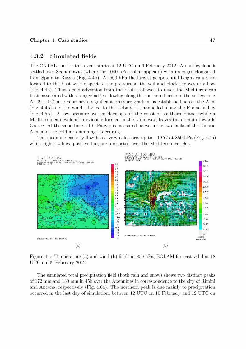
Chapter 4. Case studies 47
4.3.2 Simulated fields
The CNTRL run for this event starts at 12 UTC on 9 February 2012. An anticyclone issettled over Scandinavia (where the 1040 hPa isobar appears) with its edges elongatedfrom Spain to Russia (Fig. 4.4b). At 500 hPa the largest geopotential height values arelocated to the East with respect to the pressure at the soil and block the westerly flow(Fig. 4.4b). Thus a cold advection from the East is allowed to reach the Mediterraneanbasin associated with strong wind jets flowing along the southern border of the anticyclone.At 09 UTC on 9 February a significant pressure gradient is established across the Alps(Fig. 4.4b) and the wind, aligned to the isobars, is channelled along the Rhone Valley(Fig. 4.5b). A low pressure system develops off the coast of southern France while aMediterranean cyclone, previously formed in the same way, leaves the domain towardsGreece. At the same time a 10 hPa-gap is measured between the two flanks of the DinaricAlps and the cold air damming is occuring.
The incoming easterly flow has a very cold core, up to−19C at 850 hPa (Fig. 4.5a)while higher values, positive too, are forecasted over the Mediterranean Sea.
(a) (b)
Figure 4.5: Temperature (a) and wind (b) fields at 850 hPa, BOLAM forecast valid at 18UTC on 09 February 2012.
The simulated total precipitation field (both rain and snow) shows two distinct peaksof 172 mm and 130 mm in 45h over the Apennines in correspondence to the city of Riminiand Ancona, respectively (Fig. 4.6a). The northern peak is due mainly to precipitationoccurred in the last day of simulation, between 12 UTC on 10 February and 12 UTC on
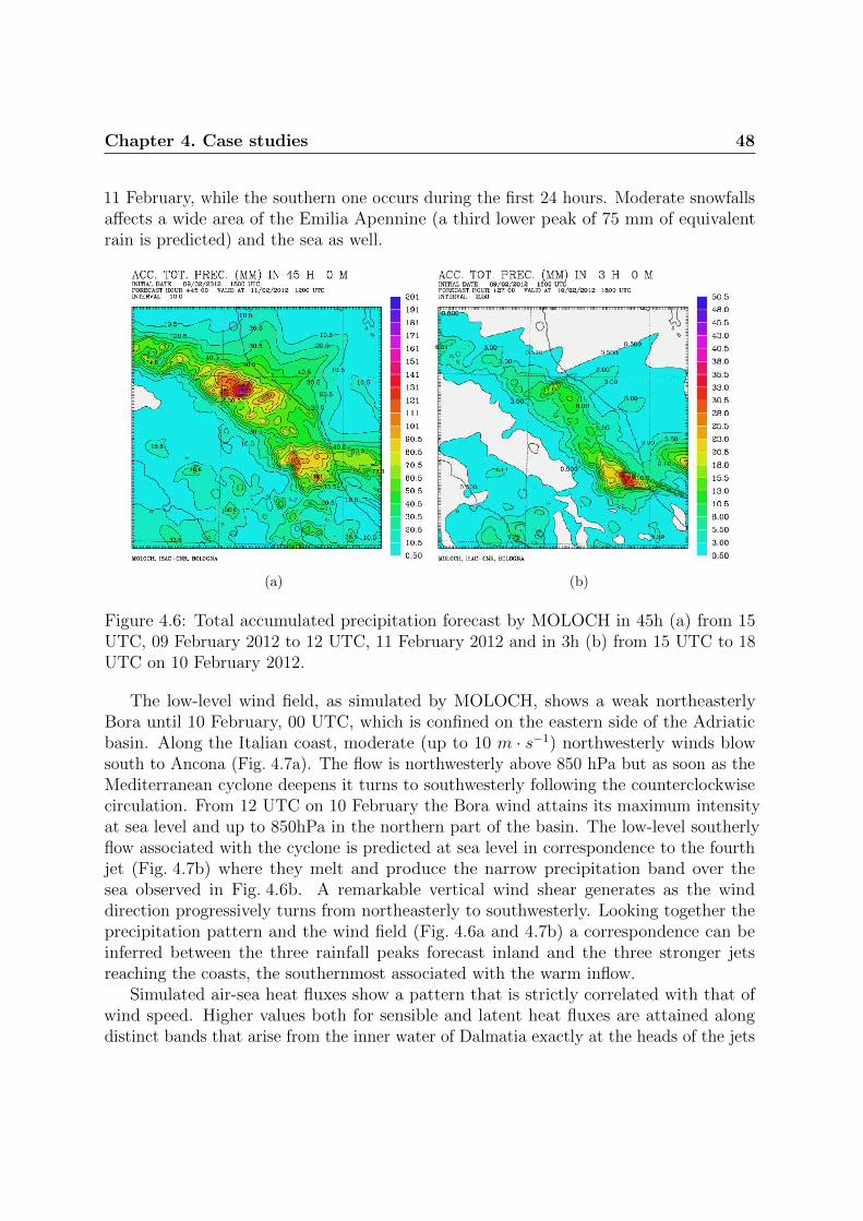
Chapter 4. Case studies 48
11 February, while the southern one occurs during the first 24 hours. Moderate snowfallsaffects a wide area of the Emilia Apennine (a third lower peak of 75 mm of equivalentrain is predicted) and the sea as well.
(a) (b)
Figure 4.6: Total accumulated precipitation forecast by MOLOCH in 45h (a) from 15UTC, 09 February 2012 to 12 UTC, 11 February 2012 and in 3h (b) from 15 UTC to 18UTC on 10 February 2012.
The low-level wind field, as simulated by MOLOCH, shows a weak northeasterlyBora until 10 February, 00 UTC, which is confined on the eastern side of the Adriaticbasin. Along the Italian coast, moderate (up to 10 m · s−1) northwesterly winds blowsouth to Ancona (Fig. 4.7a). The flow is northwesterly above 850 hPa but as soon as theMediterranean cyclone deepens it turns to southwesterly following the counterclockwisecirculation. From 12 UTC on 10 February the Bora wind attains its maximum intensityat sea level and up to 850hPa in the northern part of the basin. The low-level southerlyflow associated with the cyclone is predicted at sea level in correspondence to the fourthjet (Fig. 4.7b) where they melt and produce the narrow precipitation band over thesea observed in Fig. 4.6b. A remarkable vertical wind shear generates as the winddirection progressively turns from northeasterly to southwesterly. Looking together theprecipitation pattern and the wind field (Fig. 4.6a and 4.7b) a correspondence can beinferred between the three rainfall peaks forecast inland and the three stronger jetsreaching the coasts, the southernmost associated with the warm inflow.
Simulated air-sea heat fluxes show a pattern that is strictly correlated with that ofwind speed. Higher values both for sensible and latent heat fluxes are attained alongdistinct bands that arise from the inner water of Dalmatia exactly at the heads of the jets

Chapter 4. Case studies 49
(Fig. 4.7c-d). On average latent heat fluxes values are higher than sensible heat fluxes:istantaneous heat losses up to 1000 W ·m−2 are simulated locally.
(a) (b)
(c) (d)
Figure 4.7: Wind field forecast by MOLOCH at 03 UTC on 09 February 2012 (a) and at18 UTC on 10 February 2012 (b) at the lowest MOLOCH level (∼ 72m). Sensible (c)and latent (d) heat fluxes forecast by MOLOCH at 03 UTC on 11 February 2012.

Chapter 4. Case studies 50
4.3.3 Comparison with observations
Several weather station networks have been queried to analyse the evolution of somesurface meteorological variables namely temperature, mean sea level pressure, relativehumidity, wind speed and direction and to compare them with the values simulatedfor the MOLOCH CNTRL run on the grid points. A large number of data belongingto ARPAV, ARPA SIMC, Marche and Abruzzo regional networks have been collected.It can be said that for this case the Bora outbreak is well-predicted by the MOLOCHmodel, especially if the analysis is focused on the northern part of the domain considered(mainly to Veneto). According to MOLOCH forecast, the first Bora gusts are expectedto affect the Venetian plain by the evening of 9 February and the Po valley 2 hourslater. In Fig. 4.8 the Concordia Sagittaria (VE) wind profiler data confirms that thelow-level easterly flow starts to intensify at 19 UTC on 9 February. Data provided byradiosoundings performed at 00 UTC and 12 UTC daily at S. Pietro Capofiume (BO) areshown in Fig. 4.9: the Bora wind can be clearly identified from 00 UTC on 10 February.
Figure 4.8: SODAR data at Concordia Sagittaria (VE) wind profiler (45.76 N, 12.84 E)from 12 UTC to 18 UTC on 09 February 2012. Source: ARPAV.
Although in general a good agreement is found between model simulation and obser-vations, a couple of weather stations located more to the South is selected to show someerrors in the forecast. Fig 4.10 shows that while temperature and wind speed are in goodagreement: an increasing underestimation of the pressure and an overestimation of therelative humidity affect the first part of the simulation and this error is observed for someother stations located on the Adriatic coast. Wind speed and direction recorded andforecast in correspondence with other two weather station in central Italy are shown in

Chapter 4. Case studies 51
Figure 4.9: Radiosounding data at S. Pietro Capofiume (BO), (44.65 N, 11.62 E) collectedfrom 12 UTC, 08 February 2012 to 12 UTC, 16 February 2012. Source: ARPA SIMC.
Fig. 4.11: at Porto Recanati (AN) an important northwesterly component is not properlysimulated and at S. Benedetto del Tronto (AP) the Bora flow is overestimated in intensity,persistence and direction. This features are observed also for other weather stations inthe surrounding areas while globally the wind field forecast can be considered satisfactory.
However these inconsistencies stem for the fact that MOLOCH expectation is that ofa deeper cyclone displaced to the North so that the barrier wind south to Ancona cannot occur or, at least, are weakened (that’s why the NW component is hardly reproducedby the simulation at Porto Recanati). In that way the southernmost Bora jet is allowedto affect the coast (as forecast by MOLOCH at S. Benedetto del Tronto) while on thecontrary calm wind is recorded.
Comparing observed and forecast precipitation, a good agreement is achieved eventhough the analysis of these data is affected by relevant uncertainty due to values exceedinginstrument maximum capacities and to difficulties in getting reliable measurements bysnow-gauges. A set of significant weather stations for which data have been quality-controlled is choosen to match the total snowfall recorded with the precipitation patternsimulated in Fig. 4.6. The wide area exceeding 100 mm of equivalent rainfall over ValMarecchia and South-Romagna Apennine includes weather stations that effectively attainsnowfall of the order of one meter (Tab 4.3 - left column). A group of stations in the southto Marche experience total rainfall amounts around 50/60 mm (measured by warmedrain-gauges) and can be associated with the second peak (Tab 4.3 - right column).

Chapter 4. Case studies 52
(a)
(b)
Figure 4.10: Comparison between MOLOCH forecast and observations for wind speed,temperature, m.s.l.p. and relative humidity at (a) Mulazzano (RN) and (b) Settefonti(BO) from 15 UTC, 09 February 2012 to 12 UTC, 11 February 2012. Source: ARPASIMC.

Chapter 4. Case studies 53
(a) (b)
(c) (d)
Figure 4.11: Comparison between MOLOCH forecast and observations for wind speedand direction at (a-b) Porto Recanati (MC) and (c-d) S. Benedetto del Tronto (AP) from15 UTC, 09 February 2012 to 12 UTC, 11 February 2012. Source: C.F. Marche.
station cm/48h station cm/48h
Monzuno (BO) 73 Serravalle di Carda (PU) 73Santa Sofia (FC) 90 Urbania (PU) 122Novafeltria (RN) 117 Ancona 44
Terzo di Carnaio (FC) 105 Ripatransone(AP) 63
Table 4.3: Total snowfall amount recorded in 48h (9-11 February 2012) at selectedweather stations in Emilia Romagna (left column) and Marche (right column) regions.Shaded stations are located in the areas where MOLOCH forecast maximum rainfall.Source: [ARPA-SIMC, 2012c], [C.F.Marche, 2012b].

Chapter 4. Case studies 54
4.3.4 Sensitivity tests
Two sensitivity tests for the February case are performed varying the initial SST values, byadding and subtracting 2C, over the area displayed in Fig. 4.1. No significant differencesare observed as regards the dynamics of the event (wind speed and direction, pressureand geopotential height patterns) except for heat fluxes that are higher in the SST+simulation and lower in the SST- one (Fig. 4.12 to be compared with Fig. 4.6d). Thisbehaviour is expected since the amount of heat lost by the sea depends on the air-seatemperature difference.
What is not clearly predictable is the effect of SST variations on rainfall and snowfallsince other factors can play a role for example the incoming air stability and the boundarylayer height on the sea (see Ch. 6 for further details). In Tab. 4.4 the total precipitationamount in 45h is evaluated for each sensistivity test over selected boxes (Fig. 4.3) asthe sum of the mean hourly precipitation predicted by the model and a comparison inpercentage terms is done. It turns out that an increase (decrease) of precipitation amountover Romagna and over the Adriatic Sea of the order of 10% is expected in responseto an increasing (decreasing) SST. An opposite behaviour is observed over the centralApennines box.
(a) (b)
Figure 4.12: Latent heat fluxes for SST+ (a) and SST- (b) sensitivity tests, MOLOCHforecast valid at 03 UTC on 11 February 2012. To be compared with Fig. 4.7d.
Further tests are carried out regarding heat fluxes: at first both latent and heat fluxesare lowered to zero over northern and southern Adriatic Sea (nofluxN and nofluxS codes)

Chapter 4. Case studies 55
by applying the mask in Fig 4.2 . Then since the largest sensitivity has been observed forthe northern part of the Adriatic Sea, a further test is performed removing separatelylatent and sensible heat flux over that area only (nolatN and nosenN codes). Results interms of precipitation fields are shown in Tab. 4.4: heat fluxes have a stronger impactwith respect to SST as a drop of 60% in rainfall amount is predicted for nofluxN overthe land, mainly due to the lack of latent heat since when only laten heat flux is removed(nolatN ) almost the same value is observed. On the other hand, nosenN simulationinduces a minor effect (the decrease is no more than 20% with respect to CNTRL).
The removal of all the fluxes on the southern part of the Adriatic Sea (nofluxS )producesa precipitation decrease of 16%, 33%, 16% respectively over Romagna, Central Apennineand Adriatic Sea.
If heat fluxes are set to zero, air-sea interaction is prevented and the Bora wind isallowed to pass over the Adriatic Sea mantaining its properties: colder temperature anddrier air are expected over the Po Valley and in front of the Italian coast. After 30h frominitial time a 6C difference is observed over the Central Adriatic Sea between CNTRand nofluN simulations. Relative humidity also falls by 30% and this value is even moresignificant if considering that the maximum water vapour content of colder air is lower.
A further and more detailed analysis of the dynamical differences among the noflux -cases is proposed in Ch. 6 where cross-section are used to better understand what exactlyhappens above the sea.
February 2012
Romagna box Central Apennines box Sea boxrun mm/h var % run mm/h var % run mm/h var %
CNTRL 72.1 CNTRL 48.8 CNTRL 22.6SST+2 80.3 +11.6% SST+2 43.5 -10.7% SST+2 24.6 +8.5%SST-2 63.2 -12.3% SST-2 53.5 +9.8% SST-2 19.2 -15.1%
nofluxN 29.8 -58.6% nofluxN 19.4 -60.2% nofluxN 18.9 -16.3%nolatN 30.1 -58.3% nolatN 31.9 -34.6% nolatN 16.0 -29.2%nosenN 57.8 -19.8% nosenN 42.4 -13.1% nosenN 36.4 +61%nofluxS 60.4 -16.2% nofluxS 32.5 -33.3% nofluxS 19.0 -16%
Table 4.4: Sensitivity tests results on the precipitation field.

Chapter 4. Case studies 56
4.4 September 2012
This event is a clear example of cyclonic Bora. It has been part of the HyMeX SOP1 thataims to analyse HPE in the target area of Central Italy and a dedicated campaign (IOP-4)has been arranged with a flight, extra operational soundings and data collection. Thecyclone attains high wind speed values yielding to several convective cells developmentand total rainfall amounts of more than 300 mm over 48h as recorded on the Gran Sassomassif. A typical feature of strong cyclonic systems is observed (Fig. 4.13): as the coredeepens a cold air intrusion comes from upper levels. Globally the Central Italy is moreaffected than Emilia Romagna for this case.
Figure 4.13: MSG airmass RGB image referred to 14 September 2012 at 08.15 UTC.Source: EUMETSAT.
event initial time fcst range run code description
Sept 2012 13/09/201200 UTC
+45h
CNTR control run
SST+ SST +2 in the Adriatic Sea
SST- SST -2 in the Adriatic Sea
nofluxN both fluxes removed in the N-box
nolatN latent flux removed in the N-box
nosenN sensible flux removed in the N-box
nofluxS both fluxes removed in the S-box
Table 4.5: List and codes of the simulations performed for the September 2012 event.

Chapter 4. Case studies 57
4.4.1 Synoptic analysis
Perturbed weather conditions on mid-September 2012 affects the Mediterranean basinas a whole. It is a time-window of severe weather over Italy where two HyMeX IOP areissued in a week, the first on 12 September related to deep convection over Friuli VeneziaGiulia (IOP2) and the second, IOP4, related to the event simulated in this section.
Since early September, an anticyclonic pattern globally affected Southern and CentralEurope and this prolonged warm and moist period leads to high temperatures andhumidity values over Italy before the Bora outbreak occurs: at 06 UTC on 13 September,+18C are predicted over Sicily at 850 hPa (Fig. 4.14c). By 11 September a large-scalethrough moves from Scandinavia towards Germany and northern Italy (Fig. 4.14a). Theassociated cold front (thermal gradient more than 15 at 850hPa between incoming andpre-existing air) passes over the Alps and a lee cyclone forms over the Nortern Adriaticon 12 September and it is responsible for the high precipitation rates recorded in theNorth-East of Italy during IOP2. A second cyclone deepens between Sardinia and Corsicaby 00 UTC on 13 September and follows the typical path of Mediterranean cyclones thatis a southeasterly trajectory. It settles for a couple of days over Central Italy where itembeds the first cyclone before moving away.
(a) (b)
Figure 4.14: Geopotential height at 500 hPa (a) and mean sea level pressure (b), BOLAMforecast valid at 06 UTC on 13 September 2012.

Chapter 4. Case studies 58
4.4.2 Simulated fields
The simulation start on 13 September 2012: at 00 UTC the two cyclones are still separatedand located on different flanks of the Apennines (Fig. 4.14b). Gradually a stronger coldair intrusion from the East (e.g. the Bora wind) is induced by the cyclonic circulationwhilst in the previous days the westernmost path (northern Alps and Rhone Valley)was preferred for the flow to enter in the Mediterranean and large wind speed are stillforecasted over southern France (Fig. 4.15b). At sea level no remarkable pressure gradientis observed between the Karst Plateau and the Adriatic Sea as typical with more easterlyflows but it is enough to trigger the Bora wind possibly in response to a cold air dammingoccurring to the East of Dinaric Alps. During the following 48 hours persistent scatteredconvective precipitation affects the area close to the border between Marche and Abruzzo.Finally from 16 September onwards an high pressure ridge reinforces over Spain and thecyclone extinguishes.
(a) (b)
Figure 4.15: Temperature (a) and wind (b) fields at 850 hPa, BOLAM forecast valid at06 UTC on 13 September 2012.
The 45h-accumulated rainfall map (Fig. 4.16a) clearly shows that the eastern side ofthe Apennines and the underlying plains are affected by heavy precipitation. Globallymore than 100mm/45h are forecasted over an area approximately enclosed by Marcheborders and large precipitations are simulated also over the sea. More specifically threedistinct peaks exceeding 300mm/45h are simulated over the Apennines and a fourth

Chapter 4. Case studies 59
peaks is forecast offshore, south to Ancona. Intense rain rates are predicted as typical ofconvective phenomena: Fig. 4.16b shows this behaviour for the southern peaks for whichmore than 70% of precipitation is forecast in a 3h interval from 20 UTC to 23 UTC on13 September.
(a) (b)
Figure 4.16: Total accumulated precipitation forecast by MOLOCH in 45h (a) from 03UTC, 13 September 2012 to 00 UTC, 11 September 2012 and in 3h (b) from 20 UTC to23 UTC on 13 September 2012.
Wind fields shown in Fig.4.17a-b are referred to 03 UTC on 14 September: threeBora LLJ are simulated at both 850 hPa and 950 hPa with a weaker additional jet, thesouthernmost, which is most of the time forced by the Adriatic cyclone whose effects onwind pattern are detectable below 850 hPa. As occurred in the February 2012 case, thepresence of a low pressure system over Central Italy induces a counterclockwise circulationthat merges with the Bora flow over the central Adriatic basin. The flow blowing above850 hPa is mainly directed from the South-East at 00 UTC on 13 September over thewhole Adriatic basin but it turns completely to the East from 12 UTC in the northernAdriatic where vertical wind shear forms without the appeareance of a jet pattern. It isworth noting that in the simulation the southernmost precipitation peak is located rightin front of the coastal area where the fourth jet, and the warm moist southern inflow too,impinge.
As regards the temperature field a remarkable gradient is predicted between northernand southern Adriatic: fo example at 950hPa, at 11 UTC on 13 September, a temperatureof +11C is associated with the main Bora jet (Senj jet, the third) while in correspondence

Chapter 4. Case studies 60
(a) (b)
(c) (d)
Figure 4.17: Wind field forecast by MOLOCH at 03 UTC on 14 September 2012 at 850hPa (a) and at 950 hPa (b). Temperature field forecast at 11 UTC on 13 September 2012at 950 hPa (c) and latent heat flux forecast at 00 UTC on 14 September 2012 (d).
to the cyclonic inflow entering from the South the predicted temperature is +24C(Fig. 4.17c). This difference reflects on air-sea heat fluxes that are larger where the Borajets are simulated with narrow bands reaching locally 800 W ·m−2 but approximate to

Chapter 4. Case studies 61
zero as the line that separates the area affected by the Bora wind from that affected bycyclonic circulation is crossed (Fig. 4.17d referred to latent heat). Finally for this casean SST decrease by 1C between initial and final simulation time is predicted over thenorthern Adriatic.
4.4.3 Comparison with observations
The quality check of the MOLOCH forecasts for this event shows very good results. Theforecast starts at 00 UTC on 11 November 2013 when the Bora flow is crossing theDinaric Alps and the wind reinforces at all levels over the Adriatic basin with a very highwind speed values above 850 hPa. This agrees with the observations of the ConcordiaSagittaria wind profiler (Fig. 4.18) which is located close to the northern Adriatic coasta hundred kilometers down to the foothills of Karst Mountains: an abrupt outbreak isrecorded from midnight to 12 UTC on the same day and then a moderate easterly windregime establishes.
Figure 4.18: SODAR data at Concordia Sagittaria (VE) wind profiler (45.76 N, 12.84 E)for a 4-days time-span by the 11th September at 12 UTC. Source: ARPAV.
The mesoscale evolution is well-predicted by MOLOCH as turns out by severalcomparisons that have been done for a set of weather stations belonging mainly to Marcheregional network and concerning temperature, relative humidity, pressure and wind. Thegraphs related to four different stations are presented in Fig. 4.19 and Fig. 4.20 to showthe performances. These stations are chosen as to represent a wide areas ranging fromthe Po Valley, the Adriatic coast and up to the highest southern Apennine peak (MontePrata, 1813 m).

Chapter 4. Case studies 62
(a)
(b)
Figure 4.19: Comparison between MOLOCH forecast and observations for wind speed,temperature, m.s.l.p. and relative humidity at (a) S. Pietro Capofiume (BO) and (b)Porto Recanati (MC) from 03 UTC, 13 September 2012 to 00 UTC, 15 September 2012.Source: ARPA SIMC, C.F.Marche.
Simulated rainfalls affect mainly three areas (Fig. 4.16): the Gran Sasso massif, theTronto river basin and the hills of southern Marche and maximum values in 45h reachabout 250 mm, 370 mm and 290 mm, respectively. In Tab. 4.6 some rain-gauges located

Chapter 4. Case studies 63
(a) (b)
(c) (d)
Figure 4.20: Comparison between MOLOCH forecast and observations for wind speed anddirection at (a-b) Pesaro (PU) and (c-d) Monte Prata (AP) from 03 UTC, 13 September2012 to 00 UTC, 15 September 2012. Source: C.F. Marche.
in these areas have been considered and the shaded ones located in the areas whereMOLOCH predicts rainfall peaks. The values match except for that of Campo Imperatorewhere the observed value is 100 mm larger. Apart from individual peaks, an overviewon the actual precipitation pattern is provided by interpolated maps in Fig. 4.21 for the14th September.

Chapter 4. Case studies 64
(a) (b)
Figure 4.21: Interpolated data by Abruzzo (a) and Marche (b) Regional Agencies rain-gauges networks on 14 September 2012. Source: C.F. Marche and C.F. Abruzzo.
station mm/48h station mm/48h
Camerino (MC) 171.2 Atri (TE) 199.2
Pintura di Bolognola (MC) 274.5 Giulianova (TE) 132.8
Monte Bove (MC) 210.6 Caramanico Terme (TE) 162.6
Ripatransone (AP) 245.6 Pescara 145.2
Ascoli Piceno 225.2 Campo Imperatore (AQ) 334.8
Table 4.6: Total rainfall amount recorded in 48h from 09 UTC, 13 September 2012 to09 UTC, 15 September 2012 at selected weather stations in Marche (left column) regionand from 00 UTC, 13 September 2012 to 00 UTC, 15 September 2012 in Abruzzo (rightcolumn)region. Source: [C.F.Marche, 2012a] and C.F. Abruzzo. Shaded stations arelocated in the areas where MOLOCH forecast maximum rainfall.
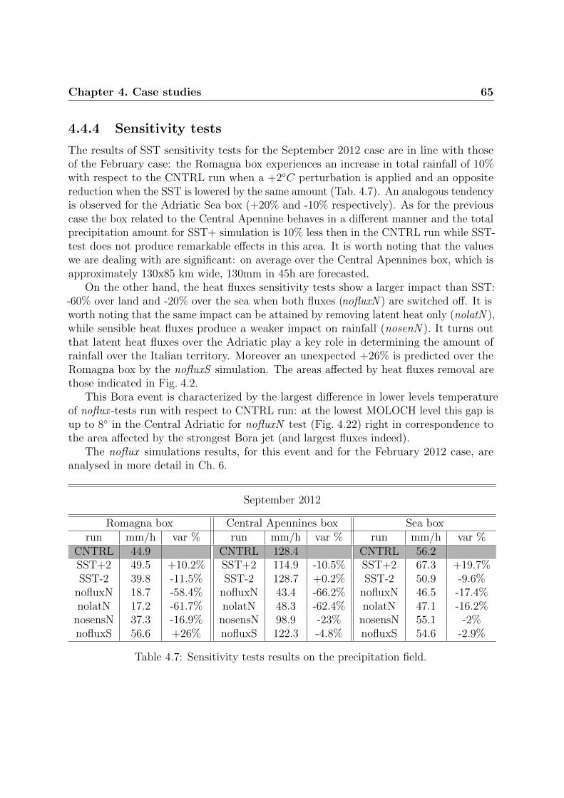
Chapter 4. Case studies 65
4.4.4 Sensitivity tests
The results of SST sensitivity tests for the September 2012 case are in line with thoseof the February case: the Romagna box experiences an increase in total rainfall of 10%with respect to the CNTRL run when a +2C perturbation is applied and an oppositereduction when the SST is lowered by the same amount (Tab. 4.7). An analogous tendencyis observed for the Adriatic Sea box (+20% and -10% respectively). As for the previouscase the box related to the Central Apennine behaves in a different manner and the totalprecipitation amount for SST+ simulation is 10% less then in the CNTRL run while SST-test does not produce remarkable effects in this area. It is worth noting that the valueswe are dealing with are significant: on average over the Central Apennines box, which isapproximately 130x85 km wide, 130mm in 45h are forecasted.
On the other hand, the heat fluxes sensitivity tests show a larger impact than SST:-60% over land and -20% over the sea when both fluxes (nofluxN ) are switched off. It isworth noting that the same impact can be attained by removing latent heat only (nolatN ),while sensible heat fluxes produce a weaker impact on rainfall (nosenN ). It turns outthat latent heat fluxes over the Adriatic play a key role in determining the amount ofrainfall over the Italian territory. Moreover an unexpected +26% is predicted over theRomagna box by the nofluxS simulation. The areas affected by heat fluxes removal arethose indicated in Fig. 4.2.
This Bora event is characterized by the largest difference in lower levels temperatureof noflux -tests run with respect to CNTRL run: at the lowest MOLOCH level this gap isup to 8 in the Central Adriatic for nofluxN test (Fig. 4.22) right in correspondence tothe area affected by the strongest Bora jet (and largest fluxes indeed).
The noflux simulations results, for this event and for the February 2012 case, areanalysed in more detail in Ch. 6.
September 2012
Romagna box Central Apennines box Sea boxrun mm/h var % run mm/h var % run mm/h var %
CNTRL 44.9 CNTRL 128.4 CNTRL 56.2SST+2 49.5 +10.2% SST+2 114.9 -10.5% SST+2 67.3 +19.7%SST-2 39.8 -11.5% SST-2 128.7 +0.2% SST-2 50.9 -9.6%
nofluxN 18.7 -58.4% nofluxN 43.4 -66.2% nofluxN 46.5 -17.4%nolatN 17.2 -61.7% nolatN 48.3 -62.4% nolatN 47.1 -16.2%
nosensN 37.3 -16.9% nosensN 98.9 -23% nosensN 55.1 -2%nofluxS 56.6 +26% nofluxS 122.3 -4.8% nofluxS 54.6 -2.9%
Table 4.7: Sensitivity tests results on the precipitation field.

Chapter 4. Case studies 66
(a) (b)
Figure 4.22: Temperature at 950 hPa for CNTRL run (a) and nofluxN run (b), MOLOCHforecast valid at 21 UTC on 13 September 2012.

Chapter 4. Case studies 67
4.5 November 2013
The November 2013 event strongly affects a large area yielding to local flood in Romagnaand Marche coastal plains and to landslides in Umbria main river basins. Such adverseimpact are not infrequent (similar effects were associated with an almost identical eventoccurred in May 2014) and are caused to the Bora impinging almost perpendicularlyon the Central Apennines. The event is also significant for a remarkable storm surgeassociated with large wave height offshore [ARPA-SIMC, 2013b]. Moreover, in this casethe slow-evolving synoptic pattern favours the persistence of severe weather conditionsfor more than 3 days, from 10 November to the end of 13 November. This cyclone is thethird that crosses the Mediterranean Sea by the beginning of the month.
It originates as a cut-off low from a through located over Central Europe, crossesrapidly from the northern Adriatic to the Tyrrhenian Sea and becomes almost stationaryin front of North Africa coast, driving the Bora flow towards the Adriatic Sea. Returnperiod between 100 and 200 years have been estimated regarding total rainfall amount atspecific rain-gauges [C.F.Umbria, 2013].
event initial time fcst range run code description
Nov 2013 11/11/201300 UTC
+45h
CNTR control run
SST+ SST +2 in the Adriatic Sea
SST- SST -2 in the Adriatic Sea
nofluxN both fluxes removed in the N-box
nolatN latent flux removed in the N-box
nosenN sensible flux removed in the N-box
nofluxS both fluxes removed in the S-box
Table 4.8: List and codes of the simulations performed for the November 2013 event.
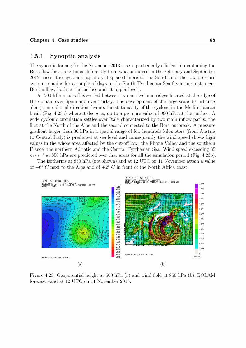
Chapter 4. Case studies 68
4.5.1 Synoptic analysis
The synoptic forcing for the November 2013 case is particularly efficient in mantaining theBora flow for a long time: differently from what occurred in the February and September2012 cases, the cyclone trajectory displaced more to the South and the low pressuresystem remains for a couple of days in the South Tyrrhenian Sea favouring a strongerBora inflow, both at the surface and at upper levels.
At 500 hPa a cut-off is settled between two anticyclonic ridges located at the edge ofthe domain over Spain and over Turkey. The development of the large scale disturbancealong a meridional direction favours the stationarity of the cyclone in the Mediterraneanbasin (Fig. 4.23a) where it deepens, up to a pressure value of 990 hPa at the surface. Awide cyclonic circulation settles over Italy characterized by two main inflow paths: thefirst at the North of the Alps and the second connected to the Bora outbreak. A pressuregradient larger than 30 hPa in a spatial-range of few hundreds kilometers (from Austriato Central Italy) is predicted at sea level and consequently the wind speed shows highvalues in the whole area affected by the cut-off low: the Rhone Valley and the southernFrance, the northern Adriatic and the Central Tyrrhenian Sea. Wind speed exceeding 35m · s−1 at 850 hPa are predicted over that areas for all the simulation period (Fig. 4.23b).
The isotherms at 850 hPa (not shown) and at 12 UTC on 11 November attain a valueof −6 C next to the Alps and of +2 C in front of the North Africa coast.
(a) (b)
Figure 4.23: Geopotential height at 500 hPa (a) and wind field at 850 hPa (b), BOLAMforecast valid at 12 UTC on 11 November 2013.

Chapter 4. Case studies 69
4.5.2 Simulated fields
The simulation starts at 00 UTC on 11 November. The total precipitation amountsforecasted in 45h are shown in Fig. 4.24a: values in excess of 300mm are indicated over along strip approximately superimposed to the highest orography, with individual peaksexceeding 500mm. The values rapidly decrease moving towards the coast especially inthe northern half of the affected area while to the South more than 100mm/45h are stillpredicted over the coastal area. The precipitation field over the sea is characterized bya band oriented from the South-East to the North-West located at the border betweenMarche and Abruzzo right along the area affected by the cyclonic circulation where theBora wind and the southern warm inflow converge. It is associated with moderate totalamount in a short time-interval. It is important to note that this convergence patternis observed for all the three cyclonic cases considered in the present work (Fig. 4.6b,Fig. 4.16b and Fig. 4.24b). Precipitations initially affects mainly the Romagna andnorthern part of Marche regions while in a second phase, during the evening of 11November, the most intense phenomena are simulated over an area among Marche,eastern Umbria and northern Abruzzo. Fig. 4.24(b) which is referred to the interval 18UTC - 21 UTC on 11 November clearly shows the typical precipitation pattern of thesecond phase of the event with severe condition to the South.
The wind field above the sea show the typical jet-pattern of Bora events: at thebeginning 5 jets can be recognised but suddenly two of them merge (Senj and Bakar jets)and finally a four-jet pattern establishes by 21 UTC on 11 November (Fig. 4.25b).

Chapter 4. Case studies 70
(a) (b)
Figure 4.24: Total accumulated precipitation forecast by MOLOCH in 45h (a) from 03UTC, 11 November 2013 to 00 UTC, 13 November 2013 and in 3h (b) from 18 UTC to21 UTC on 11 November 2013.
At variance with the previous cases, Bora affects also the central part of the Adriatic,at least in the lowest 1000 m from the surface. The cyclone is centered in the southernTyrrhenian Sea and the associated circulation is not able to confine Bora to the northernpart of the Adriatic basin (whilst it changes at 850 hPa as in Fig. 4.25a). Only at 12UTC on 12 November, when the Bora intensity decreases, the flow over the Adriatic Seaturns southeasterly at lower levels too.
The heat fluxes field shows the same features already seen for the previous cases.However the values are lower on average and latent heat fluxes attain 500 W ·m−2 andsensible heat fluxes values 250 W ·m−2 (Fig. 4.25c-d) at most.

Chapter 4. Case studies 71
(a) (b)
(c) (d)
Figure 4.25: Wind field forecast by MOLOCH at 850 hPa (a) and at 950 hPa (b), sensible(c) and latent (d) heat fluxes, valid at 18 UTC on 11 November 2013.
4.5.3 Comparison with observations
The evaluation of the forecast performances for this case and for the next ones is doneconsidering the precipitation field only. The simulated 45h-rainfall pattern (actuallysnowfall above 1800 m) is that in Fig. 4.24a and is characterized by larger values alongthe Apennines with several individual peaks and lower values on the coast. Interpolated

Chapter 4. Case studies 72
maps of rain-gauges data belonging to Marche and Umbria networks are used and confirmthat largest values are recorded next to the mountains on both the western slopes inUmbria (Fig. 4.26(a)) and the eastern slopes in Southern Marche (Fig. 4.26(b)). A set ofrain-gauges measurements is proposed in Tab. 4.9 where shaded station are located inproximity to the peaks predicted by the simulation: a great accordance is observed.
(a) (b)
Figure 4.26: Interpolated data by Umbria (a) and Marche (b) Regional Agencies rain-gauges networks for the period 00 UTC, 10 November - 00 UTC, 13 November (Umbria)and 12 UTC, 11 November - 00 UTC, 13 November (Marche). Source: [C.F.Umbria,2013], C.F. Abruzzo.
A radar reflectivity image referred to 11 November in the evening is shown in Fig. 4.27.The reflectivity peaks, that persist over the same area for several hours, matches withthe northern precipitation peak simulated by MOLOCH over Romagna Apennine. Theimage is also significant for the clearly visible pattern of parallel narrow bands of largerrainfalls, perpendicular to the Apennines, that are typical of Bora cases.

Chapter 4. Case studies 73
station mm/48h station mm/48h
Verghereto (FC) 99 Camerino (MC) 192.4
Novafeltria (RN) 90.6 Pintura di Bolognola (MC) 449.7
Gualdo Tadino (PG) 311.8 Fiastra Trebbio (MC) 441.4
Monte Cucco (PG) 248.4 Acquasanta Terme (AP) 398
Table 4.9: Total rainfall amount recorded in 48h (00 UTC, 11 November 2013 - 00 UTC,13 November 2013) at selected raing-gauges. Source: [ARPA-SIMC, 2013a], [C.F.Umbria,2013], [C.F.Marche, 2013]. Shaded stations are located in the areas where MOLOCHforecast maximum rainfall.
Figure 4.27: Radar reflectivity at 21.30 UTC on 11 November 2013 over Romagna.Source: [ARPA-SIMC, 2013b].

Chapter 4. Case studies 74
4.5.4 Sensitivity tests
The precipitation field for this case is more sensitive with respect to the two previouscyclonic cases to SST departures. Moreover it is also characterized by an unexpectedbehaviour regarding the SST- test. In particular the SST+ test is associated with a +18%of precipitation in the Romagna box (Tab. 4.10) and with a larger percentage increasein the sea box, where the average total rainfall jumps by 60% from 20mm to more than30mm in 45h with respect to CNTRL run. Together with the increase over Romagna andAdriatic Sea, a minimal decrease is once again observed as regards the Central Apenninesbox (-3%).
The behaviour of Central Appenine box is controversial since precipitation decreasesif SST is increased, but at the same time a strong increase in rainfall amount is predictedfor the sea box. This feature has been observed for all the three cyclonic Bora cases andcan be explained considering that the sea box is almost exactly located in front of theCentral Apennine box (Fig. 4.3) and that a warmer sea may favor the convection that candeplete the water vapour above the sea, thus decreasing the moisture of the air columnapproaching the coast (Fig. 4.28). This phenomenon does not happen to the North wherethe atmosphere is more stable (note that the sea box also encompasses the warmer inflowinduced by the cyclone) and the precipitation are mainly due to orographic lifting; infact no precipitation is expected above the sea beyond the 43th parallel.
(a) (b)
Figure 4.28: Total accumulated precipitation in 45h for CNTRL run (a) and SST+ run(b), MOLOCH forecast valid from 03 UTC, 11 November 2013 to 00 UTC, 13 November2013.

Chapter 4. Case studies 75
The SST- simulation, contrary to the other Bora cases discussed, still results inincreasing rainfall amounts over both Romagna and Adriatic Sea boxes while no effect isexpected for the Central Apennine box.
As regards heat fluxes sensitivity tests the November case confirms the fact thatthe removal of all the fluxes or the latent flux only has almost the same impact on theprecipitation. In particular, as observed for the other cyclonic cases, the largest effectsare simulated for the Romagna box (-30% for this case) and for the Apennines box (-15%)and the test without sensible heat flux (nosenN ) induces a change that is less than thehalf of these values (Tab. 4.10).
Finally the nofluxS simulation does not produce any interesting features on the pre-cipitation field neither it induces changes in the mesoscale pattern of northern Adriatic.Its effects have been unsignificant for the other cyclonic cases too thus it can be saidthat this specific test does not affect the area we are interested in and will not be furtherexamined in Ch. 6.
November 2013
Romagna box Central Apennines box Sea boxrun mm/h var % run mm/h var % run mm/h var %
CNTRL 65.9 CNTRL 131.3 CNTRL 19.4SST+2 78.1 +18.5% SST+2 127.6 -2.9% SST+2 30.8 +58.8%SST-2 71.7 +8.8% SST-2 130.7 -0.5% SST-2 22.1 +13.8%
nofluxN 45.4 -31% nofluxN 112.2 -14.6% nofluxN 18.9 -2.4%nolatN 45.3 -31.3% nolatN 114.2 -13% nolatN 18.1 -6.7%nosenN 55.6 -15.6% nosenN 123.2 -6.2% nosenN 19.1 -1.8%nofluxS 66.8 +1.5% nofluxS 124.5 -5.2% nofluxS 19.4 0%
Table 4.10: Sensitivity tests results on the precipitation field.

Chapter 4. Case studies 76
4.6 December 2010
This case is not so impressive for Bora severity or possible wind speed record-values butit can be considered as an ordinary Bora event. The synoptic pattern is anticyclonic withintense wind clearly detectable over the whole Adriatic basin affecting Italy from the cityof Trieste to Puglia coast. Differently from cyclonic cases the Bora flow is undisturbedsince no cyclonic inflow occurs in Central Adriatic, vertical wind-shear does not developand the convection above the sea is not favoured. Moreover a barrier wind jet, whoseorigin will be discussed, appears at the end of the forecast range.
What actually is remarkable regarding anticyclonic Bora events is that nearly allItaly, instead of the northern and central part only, experiences cold temperatures andsnowfalls (Fig. 4.29).
Figure 4.29: MODIS image of Italy on 16 December 2010 at 10.15 UTC.
event initial time fcst range run code description
Dic 2010 15/12/201000 UTC
+45hCNTR control run
noflux both fluxes removed on the sea
Table 4.11: List and codes of the simulations performed for the December 2010 event.

Chapter 4. Case studies 77
4.6.1 Synoptic analysis
The Atlantic blocking pattern is responsible for the mid-December 2010 cold spell. Fromthe geopotential height at 500 hPa and the mean sea level pressure fields it can be inferredthat the Azores High merges with an high pressure system over Greenland and allows athrough to form to the East and to move from Scandinavia to more meridional latitudes.The descent results in a first pulse of cold air that enters into the Adriatic Sea as a Boraflow on the morning of 14 December and in a second pulse with a northerly trajectorythe 17th that goes beyond the Alps and along their western side. A lee cyclon forms inthe Tyrrhenian Sea and affects Italy in the following days.
At 500 hPa low geopotential height values, associated with a slight low pressurecore at the surface, approch from the East (Fig. 4.30) while the cold inflow causes theisotherms over the Mediterranena Sea to be up to 5/6 degrees below zero at 850 hPa.The Adriatic Sea is affected by a steady easterly flow at the surface and at upper levelstoo, in the northern as well as in the southern basin (not shown). The specific timingof this event, with the Mediterranean cyclone that forms later with respect to the Boraoutbreak, makes possible to have a 48 hours of continuous Bora flow.
(a) (b)
Figure 4.30: Geopotential height at 500 hPa (a) and mean sea level pressure (b), BOLAMforecast valid at 06 UTC on 15 December 2010.

Chapter 4. Case studies 78
4.6.2 Simulated fields
The forecast range for this case includes the phenomena related to the first outbreak: thesimulation starts at 00 UTC on 15 December 2010. The precipitation amounts forecastfor the December 2010 Bora outbreak are weak and distributed over a wide area thatgoes from Romagna to Abruzzo and encompasses the sea up to a hundred km offshore(Fig. 4.31). Four peaks exceeding 45mm in 45h are predicted over the mountains butmost of the area experiences no more than 25 mm. The Apennines experiences quite allthe forecast precipitation during the first 24 hours of the simulation, until 00 UTC on 16December, while the coastal areas and the Romagna during the second day.
Figure 4.31: Total accumulated precipitation forecast by MOLOCH in 45h from 03 UTC,15 December 2010 to 00 UTC, 17 December 2010.
Th wind field shows the typical jet-pattern: actually the Trieste jet is not forecastedwhile the southernmost jets, that were prevented to form in the cyclonic cases, are nowbetter defined in the simulation even if not particularly strong. In the most intense phase,between 00 UTC and 12 UTC on 16 December, typical values are between 14 m/cdots−1
and 20 m/cdots−1 close to the eastern Adriatic coast only (Fig. 4.32a). By 12 UTC ofthe same day a sudden wind speed drop is forecasted and the wind turns to southeasterlyin front of the Apennines (from lower levels to 850 hPa) as a barrier wind. The largestrelated wind speed are simulated at 950 hPa with mean values around 15 m/cdots−1
(Fig. 4.32b).At 850 hPa the forecasted wind flow is northeasterly and moderate over the northern
Adriatic while at 700 hPa it turns slightly from the North (not shown). The wind is weakover the southern Adriatic and constant during all the period. It can be said that the

Chapter 4. Case studies 79
(a) (b)
(c) (d)
Figure 4.32: Wind field forecast by MOLOCH at lowest level (∼ 72m) at 03 UTC on 16December 2010 (a) and at 950 hPa at 17 UTC on 16 December 2010 (b). Sensible (c)and latent (d) heat fluxes forecast by MOLOCH at 03 UTC on 16 December 2010.
48 hours considered for this Bora case are affected by a sort of transition period duringwhich a weak northeasterly flow still persists over the Adriatic but is not supported atsynoptic scale where the pattern is changing in response to a through descending from
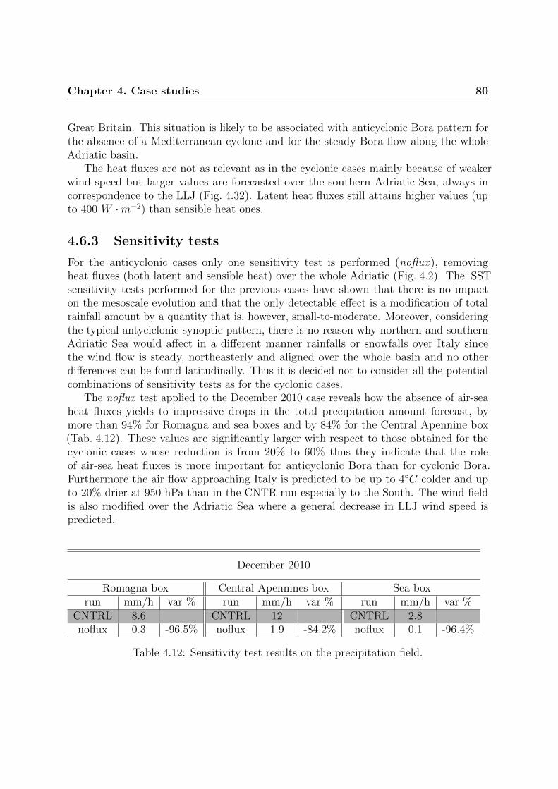
Chapter 4. Case studies 80
Great Britain. This situation is likely to be associated with anticyclonic Bora pattern forthe absence of a Mediterranean cyclone and for the steady Bora flow along the wholeAdriatic basin.
The heat fluxes are not as relevant as in the cyclonic cases mainly because of weakerwind speed but larger values are forecasted over the southern Adriatic Sea, always incorrespondence to the LLJ (Fig. 4.32). Latent heat fluxes still attains higher values (upto 400 W ·m−2) than sensible heat ones.
4.6.3 Sensitivity tests
For the anticyclonic cases only one sensitivity test is performed (noflux ), removingheat fluxes (both latent and sensible heat) over the whole Adriatic (Fig. 4.2). The SSTsensitivity tests performed for the previous cases have shown that there is no impacton the mesoscale evolution and that the only detectable effect is a modification of totalrainfall amount by a quantity that is, however, small-to-moderate. Moreover, consideringthe typical antyciclonic synoptic pattern, there is no reason why northern and southernAdriatic Sea would affect in a different manner rainfalls or snowfalls over Italy sincethe wind flow is steady, northeasterly and aligned over the whole basin and no otherdifferences can be found latitudinally. Thus it is decided not to consider all the potentialcombinations of sensitivity tests as for the cyclonic cases.
The noflux test applied to the December 2010 case reveals how the absence of air-seaheat fluxes yields to impressive drops in the total precipitation amount forecast, bymore than 94% for Romagna and sea boxes and by 84% for the Central Apennine box(Tab. 4.12). These values are significantly larger with respect to those obtained for thecyclonic cases whose reduction is from 20% to 60% thus they indicate that the roleof air-sea heat fluxes is more important for anticyclonic Bora than for cyclonic Bora.Furthermore the air flow approaching Italy is predicted to be up to 4C colder and upto 20% drier at 950 hPa than in the CNTR run especially to the South. The wind fieldis also modified over the Adriatic Sea where a general decrease in LLJ wind speed ispredicted.
December 2010
Romagna box Central Apennines box Sea boxrun mm/h var % run mm/h var % run mm/h var %
CNTRL 8.6 CNTRL 12 CNTRL 2.8noflux 0.3 -96.5% noflux 1.9 -84.2% noflux 0.1 -96.4%
Table 4.12: Sensitivity test results on the precipitation field.

Chapter 4. Case studies 81
4.7 December 2014
The event occurred at the end of 2014 is a clear example of an anticyclonic Bora patternsince the wind flow is intense all along the vertical profile and along the whole Adriaticcoast. The area affected by intense precipitation is the central and southern Apennineswindward side where moderate snowfall amount are recorded. The eastern flow lasts forseveral days, from 28 December 2014 to 02 January 2015.
As in the previous case, that of December 2010, this event does not stands out forseverity but what is peculiar is the involvement of the southern basin. Moreover, amongall the Bora events accounted in the present work, in this case we can talk about a possibleASE (see Ch. 2) since no moisture feeding is provided by outer sources but the AdriaticSea itself and snowfalls peaks are observed in inland together with typical cloud-bandspattern (Fig. 4.33).
Figure 4.33: MODIS image of Italy on 30 December 2014 at 10.15 UTC.
event initial time fcst range run code description
Dic 2014 30/12/201400 UTC
+45hCNTR control run
noflux both fluxes removed on the sea
Table 4.13: List and codes of the simulations performed for the December 2014 event.
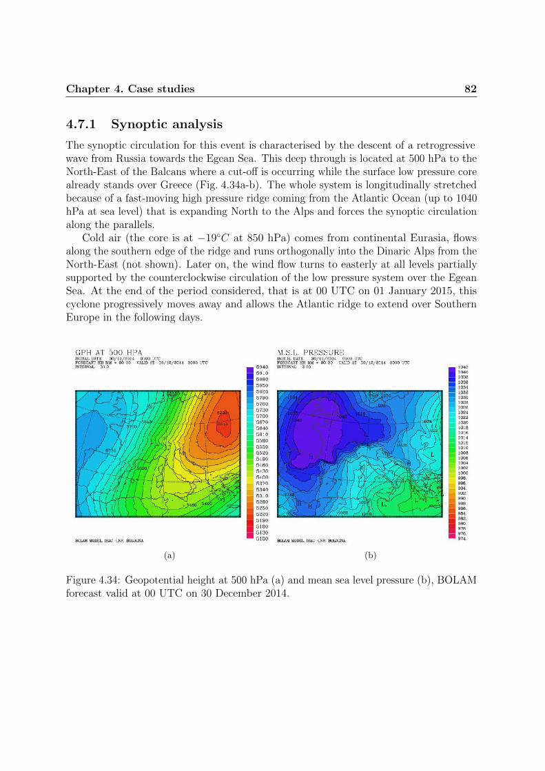
Chapter 4. Case studies 82
4.7.1 Synoptic analysis
The synoptic circulation for this event is characterised by the descent of a retrogressivewave from Russia towards the Egean Sea. This deep through is located at 500 hPa to theNorth-East of the Balcans where a cut-off is occurring while the surface low pressure corealready stands over Greece (Fig. 4.34a-b). The whole system is longitudinally stretchedbecause of a fast-moving high pressure ridge coming from the Atlantic Ocean (up to 1040hPa at sea level) that is expanding North to the Alps and forces the synoptic circulationalong the parallels.
Cold air (the core is at −19C at 850 hPa) comes from continental Eurasia, flowsalong the southern edge of the ridge and runs orthogonally into the Dinaric Alps from theNorth-East (not shown). Later on, the wind flow turns to easterly at all levels partiallysupported by the counterclockwise circulation of the low pressure system over the EgeanSea. At the end of the period considered, that is at 00 UTC on 01 January 2015, thiscyclone progressively moves away and allows the Atlantic ridge to extend over SouthernEurope in the following days.
(a) (b)
Figure 4.34: Geopotential height at 500 hPa (a) and mean sea level pressure (b), BOLAMforecast valid at 00 UTC on 30 December 2014.

Chapter 4. Case studies 83
4.7.2 Simulated fields
The simulation starts at 00 UTC on 30 December 2014. Also in this second anticycloniccase, the largest precipitation amounts are forecasted over the mountain areas (Fig. 4.35a).The precipitation field, mainly associated with snowfalls, shows a spotted pattern withpeaks (168mm and 101mm in 45h) in correspondence to the Apennines crest. The modelsimulates the precipitation along narrow bands aligned with the LLJs as already pointedout in Sec. 4.7 and Fig. 4.33 with the maximum values at their end. In Fig. 4.35b a6h-time interval has been isolated to better show this feature.
(a) (b)
Figure 4.35: Total accumulated precipitation forecast by MOLOCH in 45h (a) from 03UTC, 30 December 2014 to 00 UTC, 01 January 2015 and in 6h (b) from 21 UTC, 30December 2014 to 00 UTC, 31 December 2014.
This event affects the southern part of the Adriatic basin more than the northernone. The LLJs, also those that blow from the southern Dinaric gaps, are well-definedaccording to the simulation while at 850 hPa a northward wind-shift is forecast because ofthe forcing of the through on the large scale circulation of the South Mediterranean Sea(Fig. 4.36a). Up to 8 jets can be recognised (Fig. 4.36b), all those suggested in Sec. 2.4.2.The associated wind speeds are constantly larger than 20 m/cdots−1 for most of the timedownstream to the Dinaric Alps but only for the northern jets the wind speed remainsalmost unchanged across the Adriatic Sea up to Italy.
The Adriatic Sea surface experiences very large heat exchanges since in this case all

Chapter 4. Case studies 84
the basin is affected by a strong Bora wind. Largest values are attained all along the jettrajectories (Fig. 4.36c-d) and an impressive drop of SST by 2C in 45h globally fromthe Po delta to the Otranto channel is forecasted.
(a) (b)
(c) (d)
Figure 4.36: Wind field at 850 hPa (a) and at 950 hPa (b), sensible (c) and latent (d)heat fluxes, MOLOCH forecast valid at 09 UTC on 31 December 2014.

Chapter 4. Case studies 85
4.7.3 Sensitivity tests
The sensitivity test for the December 2014 case (noflux run) confirms the findings alreadydicussed for December 2010: the precipitation decreases to such an extent that in theRomagna box almost vanishes while the Central Appenines box experiences a fall by 78%with respect to CNTRL run (Tab. 4.14). No precipitation is predicted for the AdriaticSea box both in CNTR run and in noflux run. A significant weakening of LLJ, on averageabout 5 m/cdots−1 with respect to CNTRL run, is simulated (Fig. 4.37).
It is worth noting that for the anticyclonic cases, where no moisture feeding is providedby the cyclonic southern inflow, almost all the precipitation are due to orographic liftingin correspondence to the areas affected by strongest LLJ since, as the fluxes are setted
to zero, the rainfall decrease is dramatic. In fact, and this is the second point, the LLJweaken when heat fluxes are removed thus a crucial connection between them should beassessed (the issue is faced in Ch. 6).
Figure 4.37: Wind field forecast by MOLOCH at lowest MOLOCH level (∼ 72m) forCNTRL run (a) and noflux run (b), valid at 06 UTC on 31 December 2014.
December 2014
Romagna box Central Apennines box Sea boxrun mm/h var % run mm/h var % run mm/h var %
CNTRL 4.5 CNTRL 17.2 CNTRL 0noflux 0.1 -97.8% noflux 3.8 -77.9% noflux 0 /
Table 4.14: Sensitivity test results on the precipitation field.

Chapter 5
Profiles of water vapour fluxes andwater balance
The sensitivity tests performed for each Bora case show that air-sea heat fluxes may havea remarkable impact on the precipitation over Italy and that the largest heat fluxes areobserved in correspondence to the strongest wind speed bands. In this chapter the issue ofa better characterization of the water vapour fluxes associated with the Bora wind abovethe Sea is faced. It was observed in Ch. 4 that the horizontal propagation of the LLJ overthe Adriatic Sea may vary depending on several factors. The present chapter aims toanalyse the water vapour flux structure along the sea: in Sec. 5.1 a focus on water vapouranalysis and the diagnostic tools developed are described. In Sec. 5.2 along-coast watervapour fluxes profiles are presented while in Sec. 5.3 and 5.3.3 a complete atmosphericwater balance is carried out over the Adriatic Sea.
5.1 Diagnostic tools for water vapour flux analysis
The wind modulation over the sea, the surface heat fluxes and the SST are mutuallyconnected and vary one depending on the other via a feedback mechanism not yet fullyunderstood. An important role is played by the SST input dataset since generally in NWPmodels, and MOLOCH is no exception, the SST field is allowed to change slowly becauseof constraints to deep sea temperature and to the parametrization scheme employedfor the radiation fluxes (slab model). At the same time air-sea heat and momentumexchanges are double-acting: they strongly affect deep water mixing and Adriatic Seacirculation [Pullen et al., 2007] and they change the properties of the overhead air flowmainly raising the water vapour content and affecting the wind stress [Dorman et al.,2006].
The role of different water vapour sources (bottom fluxes or advection) is studied bymeans of two main diagnostic tools that have been developed:
86

Chapter 5. Profiles of water vapour fluxes and water balance 87
the evaluation of water vapour flux profiles, vertically integrated all along the ItalianAdriatic coast;
the computation of an atmospheric water balance over the Adriatic Sea.
In order to study the moisture flux evolution responsible for feeding heavy precipitationover the Italian shoreline and over the eastern-side of the Apennines, the evaluation ofthe water vapour flux crossing a virtual section which runs parallel to the coast is thekeypoint. This kind of analysis will give information about the total amount of watervapour moving inland towards the Apennines. However, it does not provide informationabout the sources of moisture. The characterization of moisture flux for convective casesis the focus of a series of works on severe episodes occurred over France [Nuissier et al.,2008], [Ducrocq et al., 2008], [Duffourg and Ducrocq, 2011]. The authors show that themoisture feeding the heavy precipitation systems is provided by evaporation occurred overthe Mediterranean Sea and over more distant ocean surfaces, depending on the synopticconditions established the days before the event. Moreover it is shown from a similarstudy regarding Friuli-Venezia-Giulia, that rainfalls better correlate with the mean SSTover the entire Mediterranean Sea than with the northern Adriatic only, supporting theidea that moisture coming from a large area is needed for the heaviest precipitation tooccur [Manzato, 2007].
The computation of column integrated water vapour fluxes along the eastern coast ofItaly is used to obtain information in addition to what can be deduced directly from themodel outputs. The plots of the values obtained for each grid point all together along thecoast, spanning over different heights and over the entire forecast range, give an overallview of the time and spatial evolution of the moisture inflow associated with the meaneasterly wind component over the sea.
As previously pointed out, this is not enough for a full comprehension of the fluxdynamics because informations about what happens before the water vapour impingeson the coast are still lacking and a second tool, more useful in this sense, is developed.It provides a water budget over selected volumes over the Adriatic basin, by meansof properly defined boxes, taking into account all the terms that can play a role inwater content transport. A similar study was carried out in California with the aim ofinvestigating the three-dimensional changes in water vapour fluxes associated with an“atmospheric river” [Smith et al., 2010]. A water budget approch was also applied to abox that encompasses Switzerland to find a connection between water vapour fluxes andthe extreme precipitations and floods that occured in that area in August 2005 [Koffiet al., 2013].
This kind of analysis, applied to Bora cases over the Adriatic Sea, has not been doneyet. As part of this work, the atmospheric water balance and the vertically integratedvapour fluxes computation help to focus to those local situations that deserve particularattention. For example they are helpful in positioning cross-sections and in the selectionof specific periods for comparisons among different events.

Chapter 5. Profiles of water vapour fluxes and water balance 88
5.2 Water vapour profiles along the coast
It has been explained that is crucial to have various data about the easterly flow to bettercharacterise the wind component that directly affects the Italian coast.
The water vapour flux vertically integrated up to a prescribed altitude is computedfor each grid point of the model along the Adriatic coast. The first grid point over theAdriatic sea is selected for this purposes, identified by a land-sea mask value greater than0.8. The selected coastal profile goes from Venice to the Gargano promontory (see theright side from Fig. 5.1 to Fig. 5.4).
The formula implemented in MOLOCH for the water vapour flux computation is
WV =
ztop∑i=1
wri · ρi · zi (5.1)
where wr is the rotated wind intensity, ρ is the water vapour density, z is the thicknessof each vertical layer and ztop is the top level. The equation is dimensionally-consistentsince the results are expressed in [kg ·m−1 · s−1] that is a linear istantaneous flux.
The wind field is rotated on the MOLOCH grid and wr is computed as the windcomponent perpendicular to the direction of the Apennines. Although the northernApennines present a slightly different orientation with respect to southern Apennines, amean direction for the whole orographic chain (tilted by 30° with respect to the meridian)is considered.
The flux is computed summing over all the MOLOCH vertical levels up to the pre-scribed elevation.
A textual data file is created by MOLOCH and re-arranged with Matlab to producegraphical outputs. Two different types of graphs are presented:
comparison among water vapour flux profiles referred to the same time but fordifferent altitudes of the top level;
comparison among CNTRL run and noflux runs at specific times.
In Fig. 5.1 and Fig. 5.2 the graphs belonging to the first type are presented. They arereferred to significant time instants when the strongest Bora flow is simulated, typicallyin the first part of the forecast range.
The typical multiple wind-jet pattern can be recognised in the northern part of theAdriatic basin for the cyclonic cases also in the moisture flux along the Italian coast:a three-jet structure is clearly visible for the February case (Fig. 5.1a), two jets aredistinguished for the September case (Fig. 5.1b) and four jets characterize the Novembercase (Fig. 5.2a). Among the jets the southernmost attains the largest water wapour fluxesvalues: this is clear for the February and November cases but not so well-defined for the

Chapter 5. Profiles of water vapour fluxes and water balance 89
September one for which the two jets are almost equivalent. The largest flux values arerelated to the autumn cases: the southermost September jet exceeds 350 [kg ·m−1 · s−1],the southernmost November jet is characterized by a value of 600 [kg ·m−1 · s−1] whilethe February one attains 150 [kg ·m−1 · s−1].
The separation between the northern and southern Adriatic water vapour fluxesregimes is marked in all the cyclonic events by a drop in the water vapour fluxes valuessouth of the last jet by more than half the jet value. The flux progressively raises movingsouthward and reaches another maximum.
A similar feature characterizes all the cyclonic events: the contribution to the watervapour fluxes associated with the northern Bora wind jets is mainly confined to the first1500m-2000m and very low contributions come from the upper levels. On the other hand,in the southern part of the Adriatic basin, typically south of 43 N, an opposite situationis observed: the largest contributions are those above 3000m and the flux in the firstlayers up to 500m is nearly negligible. For the November case this pattern is not sodefined and contributions above 3000m still counts for the Bora flow but a decrease inthe importance of lower layers can be noticed to the South.
Recalling that the Bora wind is merged with the warmer cyclonic circulation flow incorrespondence to the southernmost jet, a possible explanation for the observed behaviouris the following: the fact that the southernmost jet attains the largest value of the profileconfirms the hypotesis that a large part of the water vapour content comes from theSouth (from the southern Adriatic or from the Mediterranean Sea) and that the transportof moisture from large distances by the cyclonic circulation is effective. Moreover theobserved drop in water vapour fluxes is located in correspondence to the low pressurecore and the southernmost maximum observed south of the minimum is connected tothe southwesterly flow around the cyclone (since wind intensity is computed, the fluxescrossing the section from different directions always provide for a positive flux). It isworth noting that in the area affected by the Bora wind most of the contribution to theflow comes from lower levels (mainly up to 1000m), while the flow associated with thecyclonic circulation in the southern Adriatic is characterized by higher moisture contentin the upper levels, typically above 3000m.
Finally, as regards anticyclonic Bora, only the December 2014 case (which is moresignificant with respect to the December 2010 one) is presented in Fig. 5.2b. The jetpattern is clearly visible and up to 8 jets (see Fig. 4.35b for comparison) are recognised.The pattern is different since the Bora wind affects uniformly all the Adriatic basin: thecontribution up to 1000m is constant all along the coast, no drop occur and no significantwater vapour flux is predicted above 5000m for the southern jets, while a significantupper-level component characterizes the flow to the North.

Chapter 5. Profiles of water vapour fluxes and water balance 90
(a)
(b)
Figure 5.1: Water vapour flux profiles along the Italian coastline computed up to differentheights at 09 UTC on 10 February 2012 (a) and at 13 UTC on 13 September 2012 (b),MOLOCH forecast.

Chapter 5. Profiles of water vapour fluxes and water balance 91
(a)
(b)
Figure 5.2: Water vapour flux profiles along the Italian coastline computed up to differentheights at 22 UTC on 11 November 2013 (a) and at 12 UTC on 31 December 2014 (b),MOLOCH forecast.

Chapter 5. Profiles of water vapour fluxes and water balance 92
In Fig. 5.3 and Fig. 5.4 the comparison among water vapour profiles for the CNTRLrun and the noflux runs are shown for the February 2012 and September 2012 cases. Thetop level is set at 2000m.
The noflux profiles show weaker flux values than the CNTRL profile for nearly all theforecast range. Intemediate flux values between the nofluxN -nolatN and the CNTRLones are predicted for the nosenN test (sensible heat fluxes removed). The jet patternis no more clearly recognisable at the specific time instant, in the CNTRL run as well,except for the southernmost jet whose peak attains the largest values of the profile. Thispeak is forecast also for the nosenN profile while nofluxN and nolatN have globally minorfluctuations.
This behaviour is consistent with the results obtained in the sensitivity tests in Ch. 4for the precipitation field, where the largest decreases in total rainfall amount withrespect to CNTRL simulation are predicted for nofluxN and nolatN runs and the impactof nosenN run is lower. This suggests that the removal of air-sea latent heat fluxesstrongly modifies the water vapour content approaching Italy and prevents persistentsevere precipitation to occur. Actually a water vapour flux decrease can be due to lowerwater vapour content or to lower wind speed (see Eq. 5.1). The atmospheric water balanceover the Adriatic carried out in the next sections will account for this twofold issue.
South of the 43th parallel an inversion between the profiles occurs: the CNTRLrun fluxes are lower than the noflux ones. This feature is common to all the cycloniccases. Fig. 5.3b-c and Fig. 5.4b-c show the MOLOCH wind field forecast at 950 hPa forCNTRL and nofluxN runs at the time corresponding to the computation of the watervapour fluxes shown in Fig. 5.3a and Fig. 5.4a. It can be noted that, in the nofluxN runs,northwesterly barrier winds are predicted along the eastern-side of the Apennines withmoderate wind speed (up to 20 m · s−1 for the February case). Moreover the surface lowpressure core associated with the cyclone is shifted to the East with respect to CNTRLruns and is located above the Sea. The largest water vapour flux values for the nofluxcases are thus connected with the appereance of the barrier wind which gives a positivecontribution to the flux. The CNTRL run profiles values on the contrary decrease in thatarea because weak winds are predicted there as the cyclone is settled exactly over thecoastline.
In Fig. 5.5 the comparison between CNTRL run and noflux runs profiles for theanticyclonic cases are shown. The main feature is that the simulations with removedheat fluxes (both sensible and latent heat for these cases) totally loose the jet patternand no peaks are predicted for the water vapour fluxes at the coast. On the other hand,a weakening of LLJs was already noticed for the noflux simulations by the MOLOCHsensitivity tests output. This behaviour, that is common to cyclonic cases too, suggeststhat vertical heat fluxes at the Sea surface, horizontal water vapour fluxes at the Italiancoast and total precipitation amounts recorded on the Apennines are strictly connected.

Chapter 5. Profiles of water vapour fluxes and water balance 93
(a)
(b) (c)
Figure 5.3: Comparison of water vapour flux profiles along the Italian coastline up to2000m between CNTRL run and noflux -runs at 21 UTC on 10 February 2012 (a) andcorresponding MOLOCH forecasts for 950 hPa wind field for the CNTRL run (b) andthe nofluxN run (c)

Chapter 5. Profiles of water vapour fluxes and water balance 94
(a)
(b) (c)
Figure 5.4: Comparison of water vapour flux profiles along the Italian coastline up to2000m between CNTRL run and noflux -runs at 09 UTC on 14 September 2012 (a) andcorrespondinf MOLOCH forecasts for 950 hPa wind speed for the CNTRL run (b) andthe nofluxN run (c)
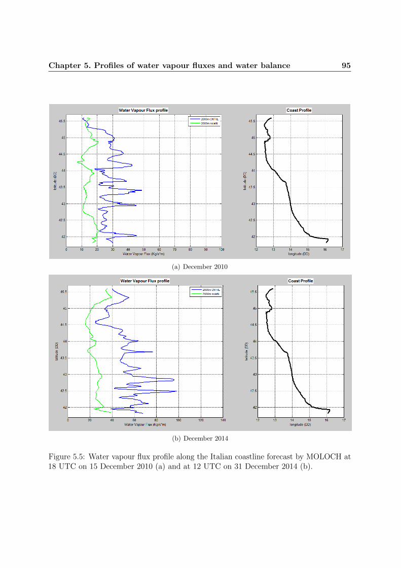
Chapter 5. Profiles of water vapour fluxes and water balance 95
(a) December 2010
(b) December 2014
Figure 5.5: Water vapour flux profile along the Italian coastline forecast by MOLOCH at18 UTC on 15 December 2010 (a) and at 12 UTC on 31 December 2014 (b).

Chapter 5. Profiles of water vapour fluxes and water balance 96
5.3 Atmospheric water balance
5.3.1 The “Adriatic box”
In order to compute the water balance over the Adriatic Sea, a 3d-rectangular box isarranged with the bottom face attached to the sea surface and the top face above thetroposphere. Different boxes are considered depending on the specific Bora case (Fig. 5.6).The choice of the key areas and the dimension of the boxes is done in order to:
include the sea surface areas where largest heat fluxes are simulated;
include the areas where largest wind speed and LLJs are simulated (that oftencoincides with the previuos case);
arrange the eastern side normal to the Bora wind and the western side parallel tothe Apennines and to the coast in order to intercept the flow feeding the rainfallinland;
The bottom face of the box is defined on the MOLOCH grid by keeping constant thenumber of grid-points for the shorther and the longer side of the rectangle, respectively.
Each contribution to the water balance entering or exiting from the box is properlycomputed as specified in Sec. 5.3.2 and the results are converted to be expressed in energyunits (Watt). Thus the values obtained are intended as total values measured across thebox. Not only water vapour but all the other hydrometeor species are considered for thefluxes computation: for example advected and falling precipitation takes into accountboth rain, snow, hail and graupel together with cloud water, cloud ice and precipitablewater. The different atmospheric water species are considered also in the IntegratedWater Vapour (IWV) content computation inside the box. Thus the balance can bereferred as an energy balance or equally as a mass balance of the atmospheric water or,as we call it hereinafter, simply water balance.
As a general rule, positive flux values mean that the flow is entering in the box whilenegative values indicate outgoing flow. This means that the Bora northeasterly flowcrossing the box provides a positive contribution on the eastern box surface and a negativecontribution on the western section.

Chapter 5. Profiles of water vapour fluxes and water balance 97
(a) (b)
(c)
Figure 5.6: Atmospheric boxes defined for the water balance computation: February case(a), September and November cases (b), December cases (c)
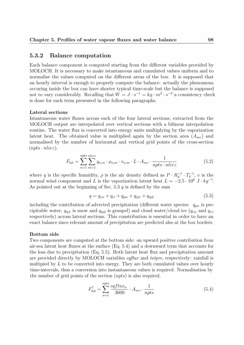
Chapter 5. Profiles of water vapour fluxes and water balance 98
5.3.2 Balance computation
Each balance component is computed starting from the different variables provided byMOLOCH. It is necessary to make istantaneous and cumulated values uniform and tonormalise the values computed on the different areas of the box. It is supposed thatan hourly interval is enough to properly compute the balance: actually the phenomenaoccuring inside the box can have shorter typical time-scale but the balance is supposednot to vary considerably. Recalling that W = J · s−1 = kg ·m2 · s−3 a consistency checkis done for each term presented in the following paragraphs.
Lateral sectionsIstantaneous water fluxes across each of the four lateral sections, extracted from theMOLOCH output are interpolated over vertical sections with a bilinear interpolationroutine. The water flux is converted into energy units multiplying by the vaporizationlatent heat. The obtained value is multiplied again by the section area (Asec) andnormalised by the number of horizontal and vertical grid points of the cross-section(npts · nlivz).
Flat =
npts∑n=1
nlivz∑m=1
qn,m · ρn,m · vn,m · L · Asec ·1
npts · nlivz(5.2)
where q is the specific humidity, ρ is the air density defined as P · R−1d · T−1V , v is the
normal wind component and L is the vaporization latent heat L = −2.5 · 106 J · kg−1.As pointed out at the beginning of Sec. 5.3 q is defined by the sum
q = qcw + qci + qpw + qip1 + qip2 (5.3)
including the contribution of advected precipitation (different water species: qpw is pre-cipitable water, qip1 is snow and qip2 is graupel) and cloud water/cloud ice (qcw and qci,respectively) across lateral sections. This constribution is essential in order to have anexact balance since relevant amount of precipitation are predicted also at the box borders.
Bottom sideTwo components are computed at the bottom side: an upward positive contribution fromair-sea latent heat fluxes at the surface (Eq. 5.4) and a downward term that accounts forthe loss due to precipitation (Eq. 5.5). Both latent heat flux and precipitation amountare provided directly by MOLOCH variables cqflux and totpre, respectively: rainfall ismultipied by L to be converted into energy. They are both cumulated values over hourlytime-intervals, thus a conversion into instantaneous values is required. Normalisation bythe number of grid points of the section (npts) is also required.
F ↑bot =
npts∑n=1
cqfluxn3600
· Asec ·1
npts(5.4)
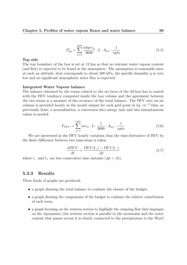
Chapter 5. Profiles of water vapour fluxes and water balance 99
F ↓bot =
npts∑n=1
totpren3600
· L · Asec ·1
npts(5.5)
Top sideThe top boundary of the box is set at 12 km so that no relevant water vapour content(and flux) is expected to be found in the atmosphere. The assumption is reasonable sinceat such an altitude, that corresponds to about 200 hPa, the specific humidity q is verylow and no significant atmospheric water flux is expected.
Integrated Water Vapour balanceThe balance obtained by the terms related to the six faces of the 3d-box has to matchwith the IWV tendency computed inside the box volume and the agreement betweenthe two terms is a measure of the accuracy of the total balance. The IWV over an aircolumn is provided hourly in the model output for each grid point in kg ·m−2 thus, aspreviously done, a normalisation, a conversion into energy unit and into instantaneousvalues is needed.
FIWV =
npts∑n=1
iwvn · L ·1
3600· Asec ·
1
npts(5.6)
We are interested in the IWV hourly variation thus the time-derivative of IWV bythe finite difference between two time-steps is taken
dIWV
dt=IWV (t+)− IWV (t−)
∆t(5.7)
where t− and t+ are two consecutive time instants (∆t = 1h).
5.3.3 Results
Three kinds of graphs are produced:
a graph showing the total balance to evaluate the closure of the budget;
a graph showing the components of the budget to evaluate the relative contributionof each term;
a graph focusing on the western section to highlight the outgoing flow that impingeson the Apennines; (the western section is parallel to the mountains and the watercontent that passes across it is clearly connected to the precipitation to the West)

Chapter 5. Profiles of water vapour fluxes and water balance 100
A 44h time-range is considered since the initial simulation instant is meaningless forthe hourly cumulated values. The IWV hourly differences are centered in the middle of theinterval while the istantaneous values are plotted hourly. To better evaluate the closure ofthe total balance the IWV differences values are inverted so that the IWV and the fluxesbalance superimpose in the figures. Figures from 5.7 to 5.11 show the three graphs foreach Bora case: total balances, separated components and the focus on the western section.
Total balance graphsThe total balance is characterized by a good closure for all the five Bora cases consideredexcept for few significant differences observed between the IWV variations (purple lines inthe (a)-panels) and the fluxes balance across the six faces (black lines) in correspondenceto peak values. The closure of the balance is not completely attained where the trendshows large fluctuations and this is true especially for the periods characterized by largeprecipitation, as can be noticed for the February 2012 case and at the end of December2010 forecast-range. Indeed, the December 2014 case, for which the bottom downwardterm due to precipitation fallout is negligible, shows the best result.
The balance of the four lateral sections together (NSWE, green lines in the (a)-panels) is negative for the anticyclonic cases and nearly close to zero with long periodscharacterized by positive values for the cyclonic events. The separated components graphswill provide an explaination for this behaviour.
The bottom upward term connected to air-sea latent heat fluxes (red line in the(a)-panels) is rather constant during the forecast range around the value of 1 · 1013W forthe February 2012, September 2012 and December 2010 cases and up to 2 · 1013 for theNovember 2013 and December 2014 cases for which actually the MOLOCH simulationsalready predicted the largest heat fluxes values over the sea among all the Bora casesconsidered (Ch. 4). The water content loss due to precipitation (blue line in the (a)-panels)is clearly higher for the cyclonic cases since heavy rainfall are simulated also over the sea,while for December 2010 and December 2014 cases, precipitation is almost negligible.
It is shown that the IWV evolution in the box agrees quite well with the totalflux balance, thus indicating a suitable closure of the water balance. However, somediscrepancies appears and may be ascribed to the following reasons:
numerical errors in the interpolation of the model variables on the lateral cross-sections;
the comparison among istantaneous values (those the of lateral sections) and integralvalues (those of the bottom face);
the fluxes across the sections are computed hourly but an higher frequency isdesirable;
the fluxes across the top side are neglected;

Chapter 5. Profiles of water vapour fluxes and water balance 101
Separated components graphsIn the separated component graphs the contribution of each face is shown individuallywhile the bottom fluxes (both upward and downward) are summed up in the term bottombalance (red line in the (b)-panels). The dominant terms (both entering or exiting) inabsolute values and the relative impact of each face with respect to the others can bediscussed looking at this kind of graph.
In particular the contribution of the northern section (green lines in the (b)-panels)results the least important. For the cyclonic cases this contribution is negative, whichmeans that an outgoing flux is established. The opposite situation is observed for theanticyclonic cases. A possible explanation is that, as already seen by analysing the windfields at different isobaric levels, the cyclonic cases are characterized by a pronouncedvertical wind shear and the prevalent wind direction over 850 hPa is basically fromthe South or the South-East over all the Adriatic basin. The anticyclonic cases on thecontrary show a more regular wind pattern with the Bora wind that blows constantlyfrom northeasterly thus it enters the box from the North or even flows parallel to theshorter box lateral sections (as in December 2014 case for which northern and southernsections have negligible flux values).
This behaviour is confirmed by the southern section trend (yellow lines in the (b)-panels). This section is crossed by the southerly flow associated with the cycloniccirculation. Large positive contributions (of the order of 1 · 1014W ) are provided by thecyclonic cases and the value increases during the event as the cyclone deepens and thecyclonic circulation reinforces.
In the February 2012 case the southern contribution equals the eastern one, associatedwith the Bora wind flow, for a 10h-period while the September 2012 and November 2013cases attain lower but significant values with respect to the total flux entering the box.On the contrary, the anticyclonic cases are characterized by negative contribution fromthe southern section or, as in December 2014, by a slightly positive one.
The eastern (purple lines in the (b)-panels) and western (light blue) sections are thoseassociated with the largest contributions. The flow is clearly an inflow from the East andan outflow from the West section with almost opposite trends. For the September 2012and November 2013 cases the eastern section contribution reaches 3 · 1014W while typicalvalues for the anticyclonic cases are one order of magnitude lower. The outflow across thewestern section is typically larger in absolute value with respect to that entering fromthe East because it gains water vapour from heat fluxes at air-sea interface and from thesouthern inflow associated with the cyclone. It is worth noting that for the cyclonic casesthe prevalent term increasing the western outgoing flow is the southern inflow while thebottom fluxes are more important for the anticyclonic cases.
It has been decided to plot the third graph with the western section separated fromthe others to highlight this crucial feature that states a significant difference between thetwo kind of Bora occurrences.

Chapter 5. Profiles of water vapour fluxes and water balance 102
West-section focusThe western section contribution (black lines in the (c)-panels) is compared with thebottom upward and downward terms and the net balance of the remaining lateral sections.Its sign is turned from negative to positive to simplify the interpretation. For the cycloniccases almost all the outgoing westward flow is balanced by the inflow from the otherlateral sections (green lines in the (c)-panels) which is mainly composed by the easterncontribution and, secondly, by the southern one. For the anticyclonic cases almost athird of the water content crossing the western section comes from heat fluxes at thebottom (red lines in the (c)-panels). While their values are almost unchanged, the relativecontribution of bottom fluxes increases for the December cases since the water flux cross-ing the lateral box boundaries is an order of magnitude lower with respect to cyclonic cases.
The role of air-sea heat fluxes turns out to be fundamental in enhancing the watercontent of the air approaching the Italian coast when an anticyclonic Bora pattern isestablished. For the cyclonic cases, on the contrary, what is critical is the atmosphericwater supply coming from the south. In general, the outgoing flux at the western sectionis larger for the cyclonic cases that are those associated with more intense precipitations.
To sum up, it has been observed that the precipitation field over the Italian coastlineand Apennines is strongly sensitive to air-sea heat fluxes over the Adriatic Sea. Aremarkable decrease of rainfall is predicted when surface heat fluxes are suppressedover the sea in the sensitivity tests for both cyclonic and anticyclonic Bora cases. Thewater vapour profile analysis along the coast shows that also the horizontal water vapourflux over the sea moving towards the Apennines decreases for these cases and that itspropagation front is no more characterized by alternated jets and wakes.
On the other hand, the atmospheric water balance computed over the sea suggeststhat the contribution to the balance due to latent heat exchanges between the sea bodyand the atmosphere (bottom face of the box) is residual with respect to the advectionterms across the lateral sections, at least for the cyclonic cases. It follows that air-seaheat fluxes effects on precipitation must be explained by a dynamical mechanism and notby hsimple mass-balance.
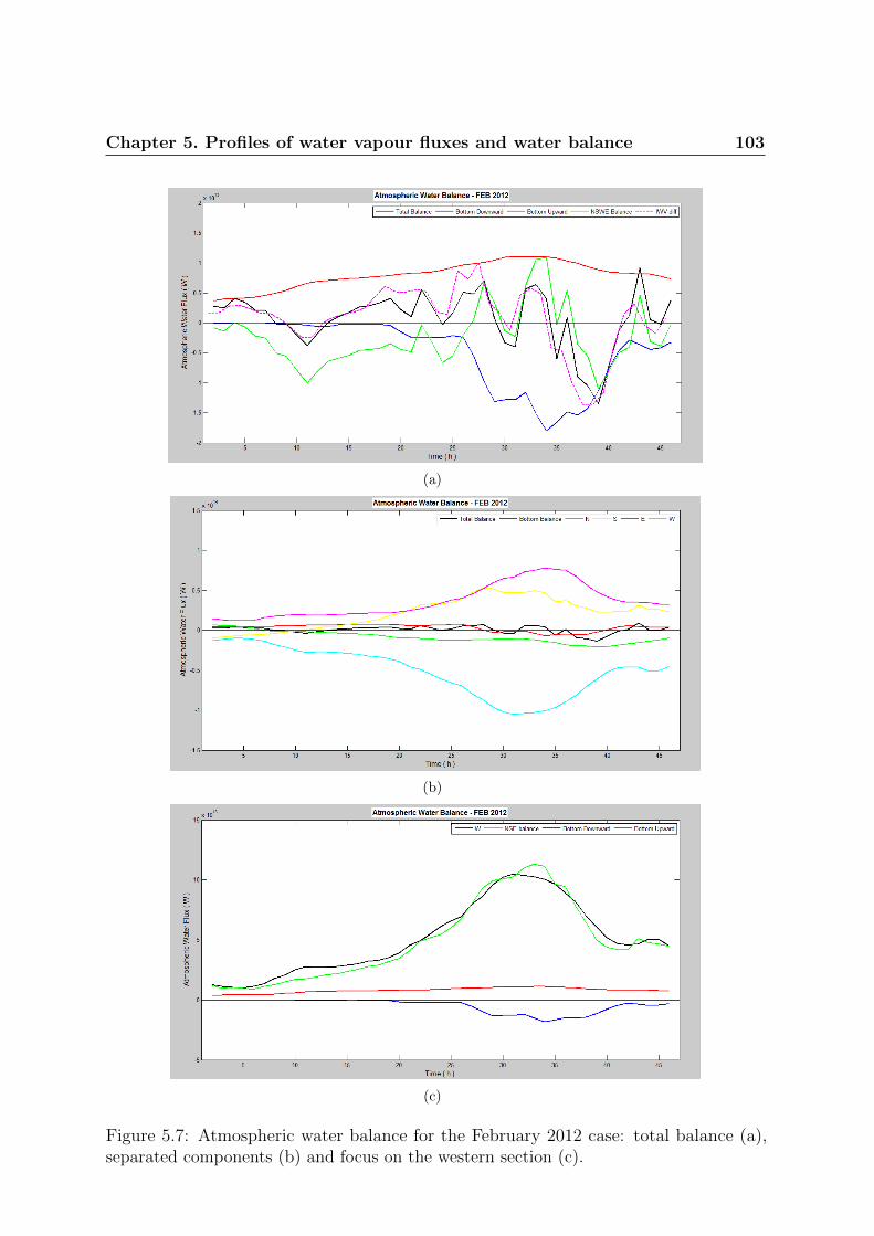
Chapter 5. Profiles of water vapour fluxes and water balance 103
(a)
(b)
(c)
Figure 5.7: Atmospheric water balance for the February 2012 case: total balance (a),separated components (b) and focus on the western section (c).

Chapter 5. Profiles of water vapour fluxes and water balance 104
(a)
(b)
(c)
Figure 5.8: Atmospheric water balance for the September 2012 case: total balance (a),individual components (b) and focus on the western section (c).

Chapter 5. Profiles of water vapour fluxes and water balance 105
(a)
(b)
(c)
Figure 5.9: Atmospheric water balance for the November 2013 case: total balance (a),individual components (b) and focus on the western section (c).

Chapter 5. Profiles of water vapour fluxes and water balance 106
(a)
(b)
(c)
Figure 5.10: Atmospheric water balance for the December 2010 case: total balance (a),individual components (b) and focus on the western section (c).

Chapter 5. Profiles of water vapour fluxes and water balance 107
(a)
(b)
(c)
Figure 5.11: Atmospheric water balance for the December 2014 case: total balance (a),individual components (b) and focus on the western section (c).

Chapter 6
Focusing on dynamics of cyclonicBora: results of numericalexperiments and discussion
This chapter faces the open question illustrated at the end of Ch. 5, that is to identifydynamical processes, associated with surface heat fluxes, affecting wind and precipitationpatterns during Bora cyclonic events. The discussion is focused on the February 2012and on the September 2012 cases that are considered as the most relevant to the issue. InSec. 6.1 the evolution of significant variables is inspected on different cross-sections locatedperpendicularly and parallel to the Bora jet trajectories. The sensitivity of MOLOCHsimulated fields to modified orography is tested in Sec. 6.2 in order to better understandthe dynamical role of orographic forcing. Final remarks are presented in Sec. 6.3.
6.1 Cross-sections
In order to assess the role of dynamical processes taking place in the atmospheric lowerlevels above the Adriatic Sea, the evolution of different meteorological variables simulatedby MOLOCH are examined on specific cross-sections arranged in prescribed key-areas.
Three different locations are considered for the cross-sections:
cross-sections over the sea, in the middle of the Adriatic;
cross-sections located approximately along the Italian coastline;
cross-sections parallel to the Bora wind jets.
The aforementioned three types of cross-sections will be referred hereinafter as to across-sea, along-coast and along-jet cross-sections.
108
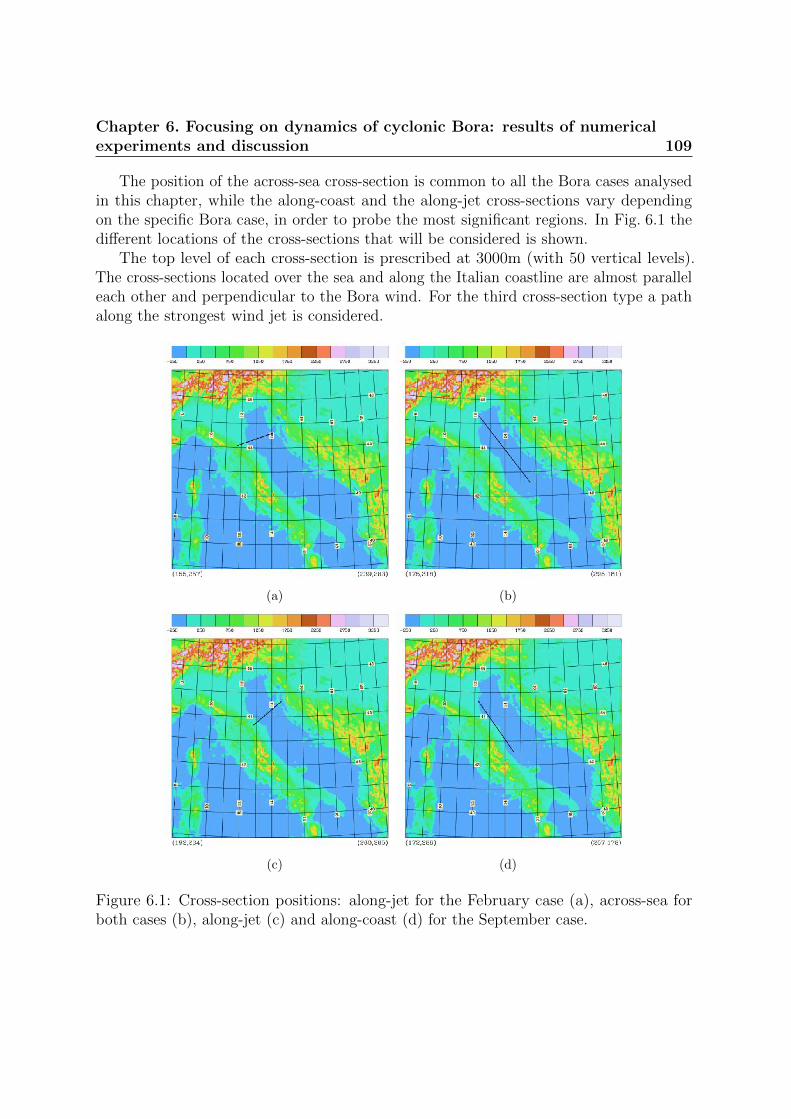
Chapter 6. Focusing on dynamics of cyclonic Bora: results of numericalexperiments and discussion 109
The position of the across-sea cross-section is common to all the Bora cases analysedin this chapter, while the along-coast and the along-jet cross-sections vary dependingon the specific Bora case, in order to probe the most significant regions. In Fig. 6.1 thedifferent locations of the cross-sections that will be considered is shown.
The top level of each cross-section is prescribed at 3000m (with 50 vertical levels).The cross-sections located over the sea and along the Italian coastline are almost paralleleach other and perpendicular to the Bora wind. For the third cross-section type a pathalong the strongest wind jet is considered.
(a) (b)
(c) (d)
Figure 6.1: Cross-section positions: along-jet for the February case (a), across-sea forboth cases (b), along-jet (c) and along-coast (d) for the September case.
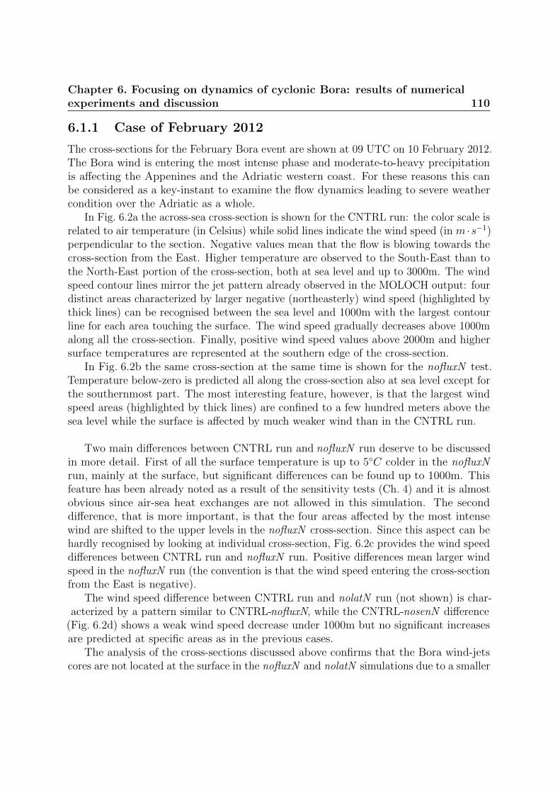
Chapter 6. Focusing on dynamics of cyclonic Bora: results of numericalexperiments and discussion 110
6.1.1 Case of February 2012
The cross-sections for the February Bora event are shown at 09 UTC on 10 February 2012.The Bora wind is entering the most intense phase and moderate-to-heavy precipitationis affecting the Appenines and the Adriatic western coast. For these reasons this canbe considered as a key-instant to examine the flow dynamics leading to severe weathercondition over the Adriatic as a whole.
In Fig. 6.2a the across-sea cross-section is shown for the CNTRL run: the color scale isrelated to air temperature (in Celsius) while solid lines indicate the wind speed (in m ·s−1)perpendicular to the section. Negative values mean that the flow is blowing towards thecross-section from the East. Higher temperature are observed to the South-East than tothe North-East portion of the cross-section, both at sea level and up to 3000m. The windspeed contour lines mirror the jet pattern already observed in the MOLOCH output: fourdistinct areas characterized by larger negative (northeasterly) wind speed (highlighted bythick lines) can be recognised between the sea level and 1000m with the largest contourline for each area touching the surface. The wind speed gradually decreases above 1000malong all the cross-section. Finally, positive wind speed values above 2000m and highersurface temperatures are represented at the southern edge of the cross-section.
In Fig. 6.2b the same cross-section at the same time is shown for the nofluxN test.Temperature below-zero is predicted all along the cross-section also at sea level except forthe southernmost part. The most interesting feature, however, is that the largest windspeed areas (highlighted by thick lines) are confined to a few hundred meters above thesea level while the surface is affected by much weaker wind than in the CNTRL run.
Two main differences between CNTRL run and nofluxN run deserve to be discussedin more detail. First of all the surface temperature is up to 5C colder in the nofluxNrun, mainly at the surface, but significant differences can be found up to 1000m. Thisfeature has been already noted as a result of the sensitivity tests (Ch. 4) and it is almostobvious since air-sea heat exchanges are not allowed in this simulation. The seconddifference, that is more important, is that the four areas affected by the most intensewind are shifted to the upper levels in the nofluxN cross-section. Since this aspect can behardly recognised by looking at individual cross-section, Fig. 6.2c provides the wind speeddifferences between CNTRL run and nofluxN run. Positive differences mean larger windspeed in the nofluxN run (the convention is that the wind speed entering the cross-sectionfrom the East is negative).
The wind speed difference between CNTRL run and nolatN run (not shown) is char-acterized by a pattern similar to CNTRL-nofluxN, while the CNTRL-nosenN difference
(Fig. 6.2d) shows a weak wind speed decrease under 1000m but no significant increasesare predicted at specific areas as in the previous cases.
The analysis of the cross-sections discussed above confirms that the Bora wind-jetscores are not located at the surface in the nofluxN and nolatN simulations due to a smaller

Chapter 6. Focusing on dynamics of cyclonic Bora: results of numericalexperiments and discussion 111
momentum mixing in the more stratfied cases, in which surface fluxes are inhibited. Thehigher temperature and the positive wind speed values above 2000m predicted at thesouthern edge of the across-sea cross-section are associated with the cyclonic circulationwhich carries warm air from the South-West. As mentioned in the water vapour profileanalysis, this flow is mainly confined to upper levels, at least in the first part of the Boraoutbreak.
The fact that the maximum wind speeds are attained at different altitudes in theCNTRL run and in the noflux -runs suggests to better examine the properties of the PBL.In order to analyse the PBL profiles over the sea the along-jet cross-section is considered.The along-jet cross-sections in Fig. 6.3 show the relative humidity field (color scale) andthe Cloud Liquid Water Ice (CLWI) content: in the CNTRL run (Fig.6.3a) a moist layerwith relative humidity values around 70% is predicted above the sea and the drier Boraflows over it in the eastern part of the section between 500m and 1000m. Values closeto saturation are observed over the mountains due to orographic uplift. In the nofluxN(Fig.6.3b) the atmosphere up to 1000m is characterised by low relative humidity (around50 %). A similar situation is predicted also in the nolatN simulation (Fig.6.3d) withrelative humidity values even lower (30% in the eastern part of the cross-section). On thecontrary, the nosenN cross-section (Fig.6.3c) shows a saturated layer 500m thick all overthe sea and over the Appenines as well.
This findings suggest that the removal of air-sea heat fluxes or latent heat flux overthe Adriatic Sea produces a Marine Boundary Layer (MBL) characterised by drier air.
On the other hand, the removal of sensible heat flux produces a wetter layer above thesea surface. The boundary layer extends up to 1000m (500m) for nofluxN and nolatN(nosenN ).
In order to better investigate the vertical stability of the PBL, potential temperature(θ) is considered on the along-jet cross-section. Fig. 6.4 shows θ distribution on thesection for CNTRL run (a-panel) and nofluxN run (b-panel), while equivalent potentialtemperature, θe, is shown in the c-panel for nosenN since in this case the first 500 metersabove the sea surface are characterized by saturation. The nolatN cross-section is notshown since it is very similar to the nofluxN one. The atmospheric stratification is largerin the nofluxN run cross-section than in the CNTRL one, where a small area next tothe coast shows an inversion of θ-values. Lower θ-values up to 1500m in the nofluxNcross-section are due to lower absolute temperature values. In the nosenN, the θe-patternshows a thicker inversion at the coast and inland where the Bora flow starts to lift overthe Apennines. The inversion of θe is a sign of instability and the fact that the nosenNrun is characterised by a more unstable layer next to the coast can explain the differentimpact that has been observed on the precipitation field: in the sensitivity tests of Ch. 4it is shown that the run with removed sensible heat flux produces a decrease of totalrainfall amount that is half the values simulated for the nofluxN and the nolatN.

Chapter 6. Focusing on dynamics of cyclonic Bora: results of numericalexperiments and discussion 112
(a) (b)
(c) (d)
Figure 6.2: Temperature and normal wind forecast by MOLOCH on the across-seacross-section for CNTRL run (a) and nofluxN run (b). CNTRL-nofluxN (c) and CNTRL-nosenN (d) wind speed differences. Continuous (dashed) lines refer to positive (negative)differences. Valid at 09 UTC on 10 February 2012.

Chapter 6. Focusing on dynamics of cyclonic Bora: results of numericalexperiments and discussion 113
(a) (b)
(c) (d)
Figure 6.3: Relative humidity and CLWI forecast by MOLOCH on the along-jet cross-section for CNTRL run (a), nofluxN run (b), nosenN run (c) and nolatN run (d), validat 09 UTC on 10 February 2012.

Chapter 6. Focusing on dynamics of cyclonic Bora: results of numericalexperiments and discussion 114
(a) (b)
(c)
Figure 6.4: Potential temperature and momentum foreacast by MOLOCH on the along-jetcross-section for CNTRL run (a) and nofluxN run (b). Equivalent potential temperature,momentum and tangential wind vectors forecast by MOLOCH on the along-jet cross-section for nosenN run. Valid at 09 UTC on 10 February 2012.
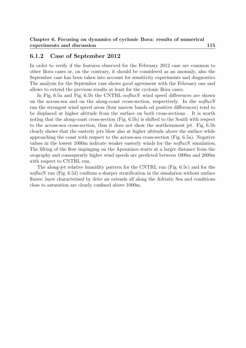
Chapter 6. Focusing on dynamics of cyclonic Bora: results of numericalexperiments and discussion 115
6.1.2 Case of September 2012
In order to verify if the features observed for the February 2012 case are common toother Bora cases or, on the contrary, it should be considered as an anomaly, also theSeptember case has been taken into account for sensitivity experiments and diagnostics.The analysis for the September case shows good agreement with the February one andallows to extend the previous results at least for the cyclonic Bora cases.
In Fig. 6.5a and Fig. 6.5b the CNTRL-nofluxN wind speed differences are shownon the across-sea and on the along-coast cross-section, respectively. In the nofluxNrun the strongest wind speed areas (four narrow bands od positive differences) tend tobe displaced at higher altitude from the surface on both cross-sections . It is worthnoting that the along-coast cross-section (Fig. 6.5b) is shifted to the South with respectto the across-sea cross-section, thus it does not show the northernmost jet. Fig. 6.5bclearly shows that the easterly jets blow also at higher altitude above the surface whileapproaching the coast with respect to the across-sea cross-section (Fig. 6.5a). Negativevalues in the lowest 1000m indicate weaker easterly winds for the nofluxN simulation.The lifting of the flow impinging on the Apennines starts at a larger distance from theorography and consequently higher wind speeds are predicted between 1000m and 2000mwith respect to CNTRL run.
The along-jet relative humidity pattern for the CNTRL run (Fig. 6.5c) and for thenofluxN run (Fig. 6.5d) confirms a sharper stratification in the simulation without surfacefluxes: layer characterised by drier air extends all along the Adriatic Sea and conditionsclose to saturation are clearly confined above 1000m.

Chapter 6. Focusing on dynamics of cyclonic Bora: results of numericalexperiments and discussion 116
(a) (b)
(c) (d)
Figure 6.5: CNTRL-nofluxN wind speed difference on the across-sea cross-section (a) andon the along-coast cross-section (b). Continuous (dashed) lines refer to positive (negative)differences. Relative humidity and CLWI for CNTRL run (c) and nofluxN run (d) onthe along-jet cross-section. Valid at 12 UTC on 14 September 2012.
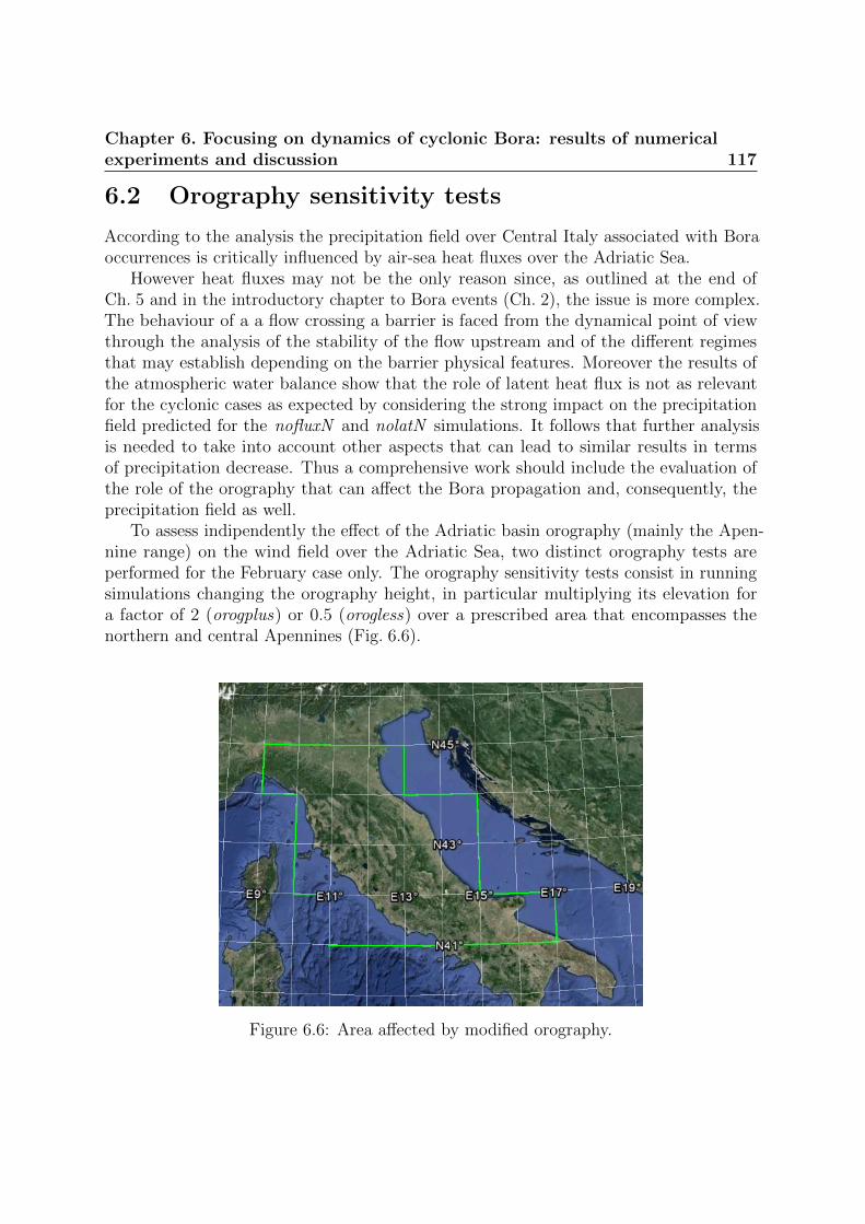
Chapter 6. Focusing on dynamics of cyclonic Bora: results of numericalexperiments and discussion 117
6.2 Orography sensitivity tests
According to the analysis the precipitation field over Central Italy associated with Boraoccurrences is critically influenced by air-sea heat fluxes over the Adriatic Sea.
However heat fluxes may not be the only reason since, as outlined at the end ofCh. 5 and in the introductory chapter to Bora events (Ch. 2), the issue is more complex.The behaviour of a a flow crossing a barrier is faced from the dynamical point of viewthrough the analysis of the stability of the flow upstream and of the different regimesthat may establish depending on the barrier physical features. Moreover the results ofthe atmospheric water balance show that the role of latent heat flux is not as relevantfor the cyclonic cases as expected by considering the strong impact on the precipitationfield predicted for the nofluxN and nolatN simulations. It follows that further analysisis needed to take into account other aspects that can lead to similar results in termsof precipitation decrease. Thus a comprehensive work should include the evaluation ofthe role of the orography that can affect the Bora propagation and, consequently, theprecipitation field as well.
To assess indipendently the effect of the Adriatic basin orography (mainly the Apen-nine range) on the wind field over the Adriatic Sea, two distinct orography tests areperformed for the February case only. The orography sensitivity tests consist in runningsimulations changing the orography height, in particular multiplying its elevation fora factor of 2 (orogplus) or 0.5 (orogless) over a prescribed area that encompasses thenorthern and central Apennines (Fig. 6.6).
Figure 6.6: Area affected by modified orography.

Chapter 6. Focusing on dynamics of cyclonic Bora: results of numericalexperiments and discussion 118
Precipitation and wind fields are considered in order to analyse the MOLOCH resultsfor the orography sensistivity tests. In the orogplus run (Fig. 6.7b) a small decrease ofthe total precipitation amount with respect to the CNTRL run (Fig. 6.7a) is simulated,in particular in the area next to the northern peak whose intensity decreases from 172mm to 138mm. The southern peak is predicted more to the East in correspondence tothe coastline where the convergence between the Bora flow and the southern cyclonic flowoccurs. On the contrary, the precipitation dramatically decreases all over the domain forthe orogless run (Fig. 6.7c): the two peaks attain 50 mm and 63 mm, respectively.
The wind field (Fig. 6.8) experiences significant changes with respect to CNTRL runas regards the crucial issue of the propagation and the strength of the Bora wind jets.In the simulation with raised orography (Fig. 6.8b) the wind jets are weaker so that thethird and the fourth ones from the North hardly affect the Italian coast. A northwesterlywind is simulated between Monte Conero promontory and Gargano promontory that hasbeen already recognised as an area favourable for barrier wind formation.
It is worth noting that the wind pattern is similar in the orogplus and nofluxNexperiments. More precisely weaker wind speeds and narrower wind bands are observedconcerning the two northernmost jets while the third and fourth jets rapidly decay andare confined in the eastern part of the Adriatic Sea. They are deflected to the South andmerge with the barrier wind developed along the coast. This pattern also inhibits the roleof the cyclonic counterclockwise flow which is conveyed towards the barrier wind insteadof impinging on the Apennines. This means that the weakening of the wind jets due tohigher orography downstream favours the flow-around regime (that is upstream blockingand flow deceleration) instead of the flow-over regime especially in correspondence to thehighest peaks which are raised up to almost 6000m in this simulation.
The orogless run (Fig. 6.8c), on the contrary, does not show significant differenceswith respect to the CNTRL run: a slight decrease in wind speed is just predicted in thesouthern part of the area affected by the Bora wind.
Fig. 6.9a and Fig. 6.9c show the wind vector on the cross-section along the jet for theorogplus and orogless simulation, respectively. The steeper orography clearly force theeasterly flow to lift at large distance from the Appenines and to reach the saturationbefore impinging on them. This behaviour can explain the fact that, although weakerjets are predicted at the coast, no significant effects are expected on the precipitationfield. On the other hand, in the orogless experiment the Bora wind blows at the lowerlevels above the sea and a slight uplift is observed inland.
Looking at the relative humidity profiles for the orography sensitivity tests it isobserved that the dry layer above the sea surface still occurs for the orogless test(Fig. 6.9d), while no significant differences with respect to CNTRL run are predicted fororogplus (Fig. 6.9b, to be compared with Fig. 6.3a). The more intense uplift observed forthe orogless experiment prevents the dry layer to form since the Bora flow is forced torise up to higher altitudes.
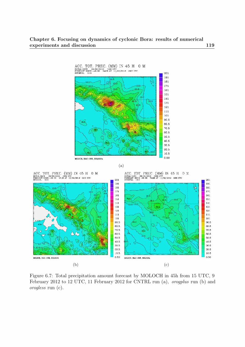
Chapter 6. Focusing on dynamics of cyclonic Bora: results of numericalexperiments and discussion 119
(a)
(b) (c)
Figure 6.7: Total precipitation amount forecast by MOLOCH in 45h from 15 UTC, 9February 2012 to 12 UTC, 11 February 2012 for CNTRL run (a), orogplus run (b) andorogless run (c).

Chapter 6. Focusing on dynamics of cyclonic Bora: results of numericalexperiments and discussion 120
(a)
(b) (c)
Figure 6.8: Wind field forecast by MOLOCH at lowest level for CNTRL run (a), orogplusrun (b) and orogless run (c), valid at 09 UTC on 10 February 2012.

Chapter 6. Focusing on dynamics of cyclonic Bora: results of numericalexperiments and discussion 121
(a) (b)
(c) (d)
Figure 6.9: θe, momentum and tangential wind vector forecast by MOLOCH on thealong-jet cross-section for orogplus (a) orogless (c) tests. Relative humidity and CLWIforecast by MOLOCH on the along-jet cross-section for the orogplus (b) and orogless (d)cases. Valid at 09 UTC on 10 February 2012.

Chapter 6. Focusing on dynamics of cyclonic Bora: results of numericalexperiments and discussion 122
6.3 Results overview
The analysis of the cross-sections carried out in this chapter allows to examine thedynamics leading to a weakening of the wind predicted over the Adriatic Sea for all thenoflux sensitivity tests. It shows that the weakening of the wind in the lowest layers, upto 500m on average, corresponds to a simultaneous increase in the wind strenght above,typically between 500m and 1000m. This feature indicates that the jet-pattern is stilloccurring even if at a different height. The relative humidity patterns on the along-jetcross-sections show that a layer with different properties establishes above the sea up to500m or more (as in the September case). For the nofluxN and nolatN (nosenN ) thelack of air-sea heat fluxes prevents the vertical mixing within the lower layer to occurand allows a drier (wetter) layer (MBL) to form. Thus the Bora wind is displaced atsome distance from the surface so that maximum speed values are no more predicted atsea level. The θ distribution on the along-jet cross-sections confirms that the MBL ischaracterised by different stability properties: it is more stable for for the nofluxN andnolatN experiments and less stable (or even locally unstable) for the nosenN one.
This feature is coherent with the precipitation field forecasts for the sensitivity tests.The sensitivity tests (Ch. 4) show that the nofluxN and nolatN runs produce similar resultsin terms of the precipitation pattern. On the contrary, the nosenN test behave differently:the decrease of total precipitation amount for this experiment is less pronounced, typicallyless than half the values predicted for nofluxN and nolatN (-20% instead of -60% for theRomagna and Appennines box and no reduction or even an increase for the sea box).This features confirms the results of the cross-section analysis: for this case the boundarylayer which develops above the sea surface is characterised by relative humidity closeto saturation (since the latent heat flux is allowed). Moreover the θe vertical gradientshows an inversion in the lowest layers of the western part of the cross-section whichindicates more favourable conditions for moist convection. Meanwhile, nofluxN andnolatN typically behave the same way.
Finally, the orography sensitivity tests show that the downstream orography (theApennines chain) also plays a crucial role. The orogplus test demonstrates that anincrease of the Appenines height implies a reduction of the Bora wind strenght and thedisappereance of the jet-pattern in the western part of the Adriatic due to the forced upliftand the development of a northwesterly barrier wind along the coast. Meanwhile, the drylayer is not observed and the precipitation field does not show significant differences withrespect to CNTRL run. As supposed, the effect of raising orography is, to some extent,similar to that obtained by removing the heat fluxes. However, this is true as regards thedynamics of the Bora wind but differences are observed concerning precipitation.
Looking at relative humidity on the along-jet cross-section no MBL establishes whenthe orography is raised, as in CNTRL run. On the contrary, in the orogless experimentdrier air penetrates at sea level too. For this case no wind speed decrease occurs but adecrease of total precipitation amount with respect to CNTRL run is predicted.

Chapter 7
Conclusions
In the present study some significant Bora events have been addressed: according to theknown distinction based on the synoptic pattern preceding the event, three cyclonic Boraepisodes and two anticyclonic Bora episodes have been considered. The MOLOCH model,nested in the BOLAM model, which, in turn, is initialized with the ECMWF analysis, isused to perform a number of simulations for each case study. The cyclonic cases turn outto be the most challenging and severe. For this reason, a large number of experimentshave been carried out for them.
The evolution of each Bora event has been analysed at the synoptic scale and, morecarefully, at the mesoscale. During the analysis, an interesting mesoscale feature hasbeen discovered for the cyclonic cases: a vertical wind shear is present over the Adriaticassociated with a southerly warm flow, blowing above the northeasterly Bora, belongingto the mesoscale circulation driven by the cyclone. The prevalent wind direction overthe Adriatic basin turns to south-southeasterly above 1500m, while the cyclonic flowmerges with the easterly Bora wind below 1500m. Typically this sharp convergence line isassociated with an intense precipitation band above the sea extending inland as well. Thepresence of a vertical wind shear for these cases characterises the common classificationinto cyclonic/anticyclonic Bora, which is mainly based on synoptic scale features.
A CNTRL run has been performed for each case study and has been compared withobservational data in order to validate the model simulations. A good agreement betweenthe simulated and the observational data has been achieved especially concerning theprecipitation forecasts, while some discrepancies have been observed for the pressure fields.The model displayed some uncertainties in simulating the location of the Adriatic cycloneand, consequently, the evolution of the meteorological fields was not always properlysimulated.
Apart from the above preliminary investigations, the main objective of the thesis isto examine the dynamics of the Bora wind over the Adriatic Sea and to identify thekey factors responsible for heavy precipitation events over the eastern Italian coast and
123

Chapter 7. Conclusions 124
the eastern flanks of the Apennines in conjunction with severe Bora outbreaks. Suchan analysis requires at first an evaluation of the role of the air-sea heat fluxes over theAdriatic which are known to provide heat and moisture to the impinging flow. Then aninvestigation of the dynamical aspects of the Bora wind propagation over the AdriaticSea has been considered.
Sensitivity tests have been performed by modifying the SST initial values for theAdriatic Sea. The increasing of the SST produced an increase of precipitation overRomagna area and over the sea and a decrease over the central Apennines. Since theair-sea temperature difference strongly affects the vapour fluxes in terms of sensibleheat flux (the larger the temperature difference, the larger the flux), this behaviour isexpected. The different impact over the Apennines is due to the fact that a warmer seamay favour the development of moist convection and the consequent depletion of thewater vapour, thus decreasing the moisture of the air column approaching the coast. Anopposite behaviour has been observed by decreasing the SST.
Additional sensitivity tests, performed by removing the air-sea heat fluxes, have beencarried out. Latent and sensible fluxes have been removed separately in the southern partof the Adriatic Sea and in the northern part. The removal of heat fluxes in the northernpart of the Adriatic Sea produces remarkable effects with respect to the CNTR run: adrop of total precipitation amount over Italy by more than 50% on average, a weakeningof the Bora wind-jet and the onset of a barrier wind along the central Italian coast. Theresults are similar when both the fluxes or latent heat only are removed. The latent heatflux over the Adriatic, in fact, is observed to be larger than the sensible heat flux duringBora events, thus its role turned out to be the most relevant.
To better understand the results of the heat flux sensitivity tests, two diagnostic toolshave been developed. The column water vapour flux along the Italian coastline has beencomputed and yielded to the following considerations. First, it shows that the horizontalwater vapour flux is mainly confined below 1500m over the North Adriatic where theBora wind blows and above 2000m over the South Adriatic where the cyclonic circulationprevails. Then the column water vapour flux shows that the southernmost Bora wind-jet,characterised by a merging with the mesoscale cyclonic flow, is the most intense amongthe different jets. This feature confirms that the water vapour coming from the Southcan strongly affect the precipitation pattern over the Apennines. Finally, it has beenobserved that the water vapour flux computed along the Italian coastline significantlydecreases in the sensistivity tests with removed heat fluxes with respect to the CNTRLrun. Also in this case, the test with latent heat flux removal behaves similarly to the testwhen both the fluxes are removed.
The second tool developed is the computation of the atmospheric water balance thathas been evaluated in a volume box over the Adriatic Sea and has demonstrated thateven if the heat fluxes (especially the latent heat flux) have a dramatic impact on theprecipitation field, their contribution to the water balance is relatively small. Moreover,

Chapter 7. Conclusions 125
considering the western section of the box, close to the Apennines, it turned out thatthe water content outflow is almost totally correlated with the contributions of the otherthree lateral sections rather than to the bottom face. This behaviour has been observedfor the cyclonic cases, while for the anticyclonic ones the contribution of the bottomlatent heat fluxes is more relevant since the advection across the lateral sections is quiteweak. Furthermore, the water balance evaluation has assessed the importance of thesouthern cyclonic flow, whose contribution to the balance is not significantly lower withrespect to that of the eastern section, which is associated with the Bora wind and it isexpected to be the largest one.
In the last chapter of the thesis a more detailed analysis of the dynamics of the Borawind over the Adriatic Sea has been carried out. In order to better understand, from adynamical point of view, the decrease of the total precipitation amount simulated for theheat flux sensitivity tests with respect to the CNTRL run, several cross-sections havebeen considered. A drier and more stable boundary layer have been observed for thoseexperiments characterized by the largest decrease in precipitation. This dry PBL abovethe Sea constrains the Bora flow at some distance above the sea surface and this patternprevents the saturation over the Sea, the coast and the foothills of the Appenines leadingto the decrease of the total precipitation amount forecast. Moreover the θ distribution onthe cross-sections has shown that a weaker stratification and a lower stability characterisethe boundary layer above the sea in the CNTRL run which is associated with heavierprecipitation.
Since the role of the dowstream orography, as discussed in Ch. 2, can be crucial inaffecting the flow propagation towards an obstacle, further sensitivity tests have beenperformed, for the February case only, to account for this issue. The orography of theMOLOCH model has been changed in order to increase and decrease the Apenninesheight. In the test with increased orography, the Bora wind is forced to lift from thesea surface up to 1500m at large distance upstream from the Apennines, just at somedistance after it descends from the Dinaric Alps slopes. The sharp ascent favours thesaturation of the air impinging on the Apennines, thus no significant decreases as regardsthe precipitation field is observed over Italy with respect to the CNTRL run. On thecontrary, diminishing the orography allows the dry Bora wind to flow at lower levels andprevents the condensation to occur over the mountains. In this case a dramatic decreasein the total precipitation amount is predicted with respect to the CNTRL run.
The evaluation of the evolution of the stability of an atmospheric layer characterisedby strong wind, intense surface heat fluxes and interacting with orography is a verycomplex issue. In the present work an empirical approach has been followed in orderto identify several mechanisms responsible for influencing the atmospheric layers duringBora wind events. In a theoretical framework a deep understanding of the role of theseprocesses can be achieved only considering individually each mechanism playing a role in

Chapter 7. Conclusions 126
the whole phenomenon. The onset of the Bora wind across the Dinaric Alps depends onthe upstream dynamics of the flow and on the barrier features. However the Bora flowaffecting Italy, once descended along the Dinaric steep slopes, is in turn influenced by theApennines. Moreover the air-sea heat fluxes and, consequently, the moisture play a rolein affecting the marine boundary layer characteristics and the properties of the boundarylayer characterise the flow upstream the Apennines. Therefore, all these processes areinvolved in an interesting and complex feedback mechanism.

Acronyms
ABL Atmospheric Boundary Layer
AdDW Adriatic Dense Water
AGU American Geophysical Union
ALPEX Alpine Experiment
AMS American Meteorological Society
ARPA Agenzia Regionale Protezione Ambiente
ASE Adriatic Sea Effect
BiOS Bimodal Oscillating System
BOLAM Bologna Limited Area Model
CAPE Convective Potential Available Energy
CFL Courant-Friedrichs-Lewy
CLWI Cloud Liquid Water Ice
CNR Consiglio Nazionale delle Ricerche
COMPARE Comparison of Mesoscale Prediction and Mesoscale Experiment
CRM Convection Resolving Model
DWF Dense Water Formation
ECMWF European Centre for Medium-range Weather Forecast
GFS Global Forecast System
GM Global Model
127

HyMeX HYdrological MEditerranean Cycle
HP High Pressure
HPE High Precipitation Events
IFS Integrated Forecast System
IOP Intesive Observation Period
ISAC Istituto di Scienze dell’Atmosfera e del Clima
ISMAR Istituto di Scienze MARine
IWV Integrated Water Vapour
LAM Limited Area Model
LCL Lifting Condensation Level
LIW Levantine Intermediate Water
LLJ Low Level Jets
LP Low Pressure
LW Long Wave
LES Lake-Effect Snow
MAP Mesoscale Alpine Project
MBL Marine Boundary Layer
McICA Monte-Carlo Independent Column Approximation
MCS Mesoscale Convective System
MOLOCH MOdello LOCale in coordinate H
NAdDW North Adriatic Dense Water
NCAR National Center for Atmospheric Research
NCEP National Centers for Environmental Prediction
NCL NCAR Command Language
NWP Numerical Weather Prediction
128

PBL Planetary Boundary Layer
PDE Partial Differential Equation
PV Potential Vorticity
QPF Quantitative Precipitation Forecast
RISKMED Weather Risk Reduction for the Mediterannean
RITMARE Ricerca Italiana per il Mare
RRTM Rapid Radiative Transfer Model
SAP South Adriatic Pit
SAR Synthetic-aperture radar
SODAR SOnic Detection And Ranging
SOP Special Observation Period
SST Sea Surface Temperature
SW Short Wave
SWH Significant Wave Height
TKE Turbulence Kinetic Energy
UKMO United Kingdom Meteorological Office
UTC Universal Time Coordinated
WAC Western Adriatic Current
WAF Weighted Average Flux
WMO World Meteorological Organization
129

References
[Alpers et al., 2009] Alpers, W., A.Ivanov, and J.Horstmann (2009). Observations ofBora Events over the Adriatic Sea and Black Sea by Spaceborne Synthetic ApertureRadar. Monthly Weather Review, 137(3).
[Arakawa and Lamb, 1977] Arakawa, A. and Lamb, V. (1977). Computational design ofthe basic dynamical processes of the UCLA general circulation model, chapter 17, pages173–265. Academic Press.
[ARPA-SIMC, 2012a] ARPA-SIMC (2012a). Le nevicate di Febbraio 2012: i dati disponi-bili. Technical report, ARPA Emilia Romagna - Servizio IdroMeteoClima - Area Retidi Monitoraggio.
[ARPA-SIMC, 2012b] ARPA-SIMC (2012b). Rapporto dell’evento meteorologico dal 31Gennaio al 5 Febbraio 2012 . Technical report, ARPA Emilia Romagna - ServizioIdro-Meteo-Clima.
[ARPA-SIMC, 2012c] ARPA-SIMC (2012c). Rapporto dell’evento meteorologico dal 7 al12 Febbraio 2012 . Technical report, ARPA Emilia Romagna - Servizio Idro-Meteo-Clima.
[ARPA-SIMC, 2013a] ARPA-SIMC (2013a). Annali Idrologici 2013.
[ARPA-SIMC, 2013b] ARPA-SIMC (2013b). Rapporto dell ’evento idrologico e meteo-marino del 10-12 novembre 2013 . Technical report, ARPA Emilia Romagna - ServizioIdro-Meteo-Clima.
[Artegiani et al., 1997] Artegiani, A., Paschini, E., and Russo, A. (1997). The AdriaticSea general circulation. Part I: Air-sea interactions and water mass structure.
[Askari et al., 2003] Askari, F., Signell, R., and Chiggiato, J. (2003). RADARSATmapping of Bora/Sirocco winds in the Adriatic Sea.
[Barker et al., 2008] Barker, H. W., Cole, J. N. S., Morcrette, J.-J., Pincus, R., Raisanen,P., von Salzen, K., and Vaillancourt, P. A. (2008). The Monte Carlo Independent
130

Column Approximation: an assessment using several global atmospheric models.Quarterly Journal of the Royal Meteorological Society, 134(635):1463–1478.
[Bartzokas et al., 2010] Bartzokas, A., Azzopardi, J., Bertotti, L., Buzzi, A., Cavaleri,L., Conte, D., Davolio, S., Dietrich, S., Drago, A., Drofa, O., Gkikas, A., Kotroni, V.,Lagouvardos, K., Lolis, C. J., Michaelides, S., Miglietta, M., Mugnai, A., Music, S.,Nikolaides, K., Porcu, F., Savvidou, K., and Tsirogianni, M. I. (2010). The RISKMEDproject: philosophy, methods and products. Natural Hazards and Earth System Science,10(7):1393–1401.
[Belusic et al., 2013] Belusic, D., Hrastinski, M., Vecenaj, Z., and Grisogono, B. (2013).Wind Regimes Associated with a Mountain Gap at the Northeastern Adriatic Coast.Journal of Applied Meteorology and Climatology.
[Billet and Toro, 1997] Billet, S. J. and Toro, E. F. (1997). On the Accuracy and Stabilityof Explicit Schemes for Multidimensional Linear Homogeneous Advection Equations.Journal of Computational Physics, 131(1).
[Blackadar, 1962] Blackadar, A. K. (1962). The vertical distribution of wind and turbulentexchange in a neutral atmosphere. Journal of Geophysical Research, 67(8):3095–3102.
[Bougeault et al., 2001] Bougeault, P., Binder, P., Buzzi, A., and Dirks, R. (2001). TheMAP special observing period.
[Bougeault and Lacarrere, 1989] Bougeault, P. and Lacarrere, P. (1989). Parameteriza-tion of orographic induced turbulence in a mesobeta scale model. Monthly WeatherReview, 117:1872–1890.
[Buzzi et al., 2003] Buzzi, A., D’Isidoro, M., and Davolio, S. (2003). A case-study of anorographic cyclone south of the Alps during the MAP SOP. Quarterly Journal of theRoyal Meteorological Society, 129(591):1795–1818.
[Buzzi et al., 1994] Buzzi, A., Fantini, M., Malguzzi, P., and Nerozzi, F. (1994). Valida-tion of a limited area model in cases of mediterranean cyclogenesis: Surface fields andprecipitation scores. Meteorology and Atmospheric Physics, 53(3-4):137–153.
[Buzzi and Foschini, 2000] Buzzi, A. and Foschini, L. (2000). Mesoscale Meteorolog-ical Features Associated with Heavy Precipitation in the Southern Alpine Region.Meteorology and Atmospheric Physics, 72(2-4):131–146.
[Calwagen, 1926] Calwagen, E. G. (1926). Zur Diagnose und Prognose lokaler Som-merschauer Aerologische Flugzeugaufstiege in Ostnorwegen. Oslo CammermeyersBoghandel.
131

[Camuffo, 1981] Camuffo, D. (1981). Fluctuation in wind direction at Venice, related tothe origin of the air masses.
[Camuffo, 1990] Camuffo, D. (1990). Acidic Precipitation Research in Italy, volume 5 ofAdvances in Environmental Science. Springer New York.
[Cavaleri et al., 2010] Cavaleri, L., Bertotti, L., Buizza, R., Buzzi, A., Masato, V.,Umgiesser, G., and Zampieri, M. (2010). Predictability of extreme meteo-oceanographicevents in the Adriatic Sea. Quarterly Journal of the Royal Meteorological Society,136(647):400–413.
[Cesini et al., 2004] Cesini, D., Morelli, S., and Parmiggianil, F. (2004). Analysis of anintense bora event in the Adriatic area. Natural Hazards and Earth System Science,4(2):323–337.
[C.F.Marche, 2012a] C.F.Marche (2012a). Annali Idrologici 2012 .
[C.F.Marche, 2012b] C.F.Marche (2012b). Rapporto di evento 1-13 Febbraio 2012 .Technical report, Regione Marche - Dipartimento per le politiche integrate di sicurezzae per la protezione civile - Centro funzionale per la meteorologia, l’idrologia e lasismologia.
[C.F.Marche, 2013] C.F.Marche (2013). Rapporto di evento 10-13 Novembre 2013 .Technical report, Regione Marche - Dipartimento per le politiche integrate di sicurezzae per la protezione civile - Centro funzionale per la meteorologia, l’idrologia e lasismologia.
[C.F.Umbria, 2013] C.F.Umbria (2013). Evento alluvionale 11-12 Novembre 2013 - Rap-porto d’evento . Technical report, Regione Umbria - Direzione Programmazione,Innovazione e Competitivita dell’Umbria - Servizio Protezione Civile - Centro Fun-zionale.
[Charnock, 1955] Charnock, H. (1955). Wind stress on a water surface. Quarterly Journalof the Royal Meteorological Society, 81(350):639–640.
[Davolio et al., 2007] Davolio, S., Buzzi, A., and Malguzzi, P. (2007). High resolutionsimulations of an intense convective precipitation event. Meteorology and AtmosphericPhysics, 95(3-4):139–154.
[Davolio et al., 2009a] Davolio, S., Mastrangelo, D., Miglietta, M., Drofa, O., Buzzi, A.,and Malguzzi, P. (2009a). High resolution simulations of a flash flood near Venice.Natural Hazards and Earth System Science, 9(5):1671–1678.
132

[Davolio et al., 2009b] Davolio, S., Miglietta, M. M., Moscatello, A., Pacifico, F., Buzzi,A., and Rotunno, R. (2009b). Numerical forecast and analysis of a tropical-like cyclonein the Ionian Sea. Natural Hazards and Earth System Science, 9(2):551–562.
[Davolio et al., 2015] Davolio, S., Stocchi, P., Benetazzo, A., Bohm, E., Riminucci, F.,Ravaioli, M., Li, X.-M., and Carniel, S. (2015). Exceptional Bora outbreak in winter2012: validation and analysis of high-resolution atmospheric model simualtions in thenorthern Adriatic Area.
[Davolio et al., 2013] Davolio, S., Stocchi, P., Miglietta, M., Buzzi, A., Malguzzi, P.,Fantini, M., and Drofa, O. (2013). RITMARE - Ricerca ITaliana per il MARE: primavalidazione dei modelli atmosferici.
[Dorman et al., 2006] Dorman, C., , and and (2006). February 2003 marine atmosphericconditions and the bora over the northern Adriatic. Journal of Geophysical Research,112(C3).
[Drobinski, 2014] Drobinski, P. e. a. (2014). HyMeX: A 10-Year Multidisciplinary Pro-gram on the Mediterranean Water Cycle. Bulletin of the American MeteorologicalSociety, 95(7).
[Drofa and Malguzzi, 2004] Drofa, O. and Malguzzi, P. (2004). Parameterization ofmicrophysical processes in a non hydrostatic prediction model. In Proc. 14th Intern.Conf. on Clouds and Precipitation (ICCP).
[Ducrocq et al., 2008] Ducrocq, V., Nuissierl, O., Ricardl, D., Lebeaupinl, C., and Thou-venin, T. (2008). A numerical study of three catastrophic precipitating events oversouthern France. II: Mesoscale triggering and stationarity factors. Quarterly Journalof the Royal Meteorological Society, 134(630):131–145.
[Ducrocq, 2014] Ducrocq, V. e. a. (2014). HyMeX-SOP1: The Field Campaign Dedicatedto Heavy Precipitation and Flash Flooding in the Northwestern Mediterranean. Bulletinof the American Meteorological Society, 95(7).
[Duffourg and Ducrocq, 2011] Duffourg, F. and Ducrocq, V. (2011). Origin of the mois-ture feeding the heavy precipitating systems over southeastern France. Natural Hazardsand Earth System Science, 11(4):1163–1178.
[Durran, 1990] Durran, D. (1990). Mountain Waves and Downslope Winds.
[Enger and Grisogono, 1998] Enger, L. and Grisogono, B. (1998). The response of boratype flow to sea surface temperature.
133

[Ferrarese et al., 2009] Ferrarese, S., Cassardol, C., Elmi, A., Genovese, R., Longhetto,A., M-Manfrin, and Richiardone, R. (2009). Air-sea interactions in the Adriatic Basin:simulations of Bora and Sirocco wind events. Geofizika, 26(2).
[Ferrarin et al., 2013] Ferrarin, C., Roland, A., Bajo, M., Umgiesser, G., Cucco, A.,Davolio, S., Buzzi, A., Malguzzi, P., and Drofa, O. (2013). Tide-surge-wave modellingand forecasting in the Mediterranean Sea with focus on the Italian coast . OceanModelling, 61(0):38 – 48.
[Ferretti, 2014] Ferretti, R. e. a. (2014). Overview of the first HyMeX Special ObservationPeriod over Italy: observations and model results. Hydrology and Earth System Sciences,18(5):1953–1977.
[Gabersek and Durran, 2004] Gabersek, S. and Durran, D. (2004). Gap flows throughidealized topography. Part I: Forcing by large-scale winds in the nonrotating limit.Journal of the Atmospheric Sciences, 61(23):2846–2862. cited By 26.
[Gacic et al., 2010] Gacic, M., Borzelli, G. L. E., Civitarese, G., Cardin, V., and Yari, S.(2010). Can internal processes sustain reversals of the ocean upper circulation? theionian sea example. Geophysical Research Letters, 37(9):n/a–n/a.
[Gohm, Alexander and Mayr, Georg J. and Fix, Andreas and Giez, Andreas, 2008]Gohm, Alexander and Mayr, Georg J. and Fix, Andreas and Giez, Andreas (2008).On the onset of bora and the formation of rotors and jumps near a mountain gap.Quarterly Journal of the Royal Meteorological Society, 134(630):21–46.
[Grazzini, 2013] Grazzini, F. (2013). Cold spell prediction beyond a week: extremesnowfall events in February 2012 in Italy. ECMWF Newsletters, (136).
[Grisogono and Belusic, 2009] Grisogono, B. and Belusic, D. (2009). A review of recentadvances in understanding the meso- and microscale properties of the severe Bora wind.Tellus A, 61(1).
[Grubisıc, 2004] Grubisıc, V. (2004). Bora-driven potential vorticity banners over theAdriatic. Quarterly Journal of the Royal Meteorological Society, 130(602):2571–2603.
[Grubisic and Orlic, 2007] Grubisic, V. and Orlic, M. (2007). Early Observations ofRotor Clouds by Andrija Mohorovicic.
[Horvath et al., 2009] Horvath, K., Ivatek-Sahdan, S., Ivancan-Picek, B., and Grubisic,V. (2009). Evolution and Structure of Two Severe Cyclonic Bora Events: Contrastbetween the Northern and Southern Adriatic. Weather and Forecasting, 24(4).
134

[Janecovic et al., 2014] Janecovic, I., Mihanovic, I., I.Vilibic, and M.Tudor (2014). Ex-treme cooling and dense water formation estimates in open and coastal regions of theAdriatic Sea during the winter of 2012. Journal of Geophysical Research: Oceans,119(5).
[Jeffries and Lee, 2007] Jeffries, M. and Lee, C. M. (2007). A climatology of the northernAdriatic Sea response to bora and river forcing. Journal of Geophysical Research:Oceans (1978–2012), 112(C3).
[Jiang and Doyle, 2005] Jiang, Q. and Doyle, J. D. (2005). Wave breaking induced surfacewakes and jets observed during a bora event. Geophysical Research Letters, 32(17).
[Jurcec, 1981] Jurcec, V. (1981). On mesoscale characteristics of bora conditions inyugoslavia. In Liljequist, G., editor, Weather and Weather Maps, Contributions toCurrent Research in Geophysics, pages 640–657. Birkhauser Basel.
[Kain, 2004] Kain, J. (2004). The Kain-Fritsch convective parameterization: an update.
[Kain and Fritsch, 1990] Kain, J. S. and Fritsch, J. M. (1990). A One-Dimensional En-training/Detraining Plume Model and Its Application in Convective Parameterization.Journal of the Atmospheric Science, 47:2784–2802.
[Koffi et al., 2013] Koffi, E. N., Graham, E., and Matzler, A. (2013). The water vapourflux above Switzerland and its role in the August 2005 extreme precipitation andflooding. Meteorologische Zeitschrift, 22(3):328–341.
[Kraljevic and Grisogono, 2006] Kraljevic, L. and Grisogono, B. (2006). Sea-surfacetemperature effects on 3D bora-like flow. Meteorologische Zeitschrift, 15(2).
[Kuzmic et al., 2013] Kuzmic, M., Li, X., Grisogono, B., Tomazic, I., and Lehner, S.(2013). TerraSAR-X observations of the northeastern Adriatic bora: early results.
[Lazic and Tosic, 1997] Lazic, L. and Tosic, I. (1997). A real data simulation of theAdriatic bora and the impact of mountain height on bora trajectories. Meteorologyand Atmospheric Physics, 66(3):143–155.
[Lebeaupin et al., 2006] Lebeaupin, C., Ducrocq, V., and Giordani, H. (2006). Sensitivityof torrential rain events to the sea surface temperature based on high-resolutionnumerical forecasts. Journal of Geophysical Research: Atmospheres, 111(D12):n/a–n/a.
[Lehmann, 1993] Lehmann, R. (1993). On the choice of relaxation coefficients for Davies’lateral boundary scheme for regional weather prediction models. Meteorology andAtmospheric Physics, 52(1-2):1–14.
135

[Lionello et al., 2012] Lionello, P., Cavaleri, L., Nissen, K., Pino, C., Raicich, F., andUlbrich, U. (2012). Severe marine storms in the Northern Adriatic: Characteristicsand trends. Physics and Chemistry of the Earth, Parts A/B/C, 40-41.
[Ludwig et al., 2014] Ludwig, P., Pinto, J. G., Reyers, M., and Gray, S. L. (2014). Therole of anomalous SST and surface fluxes over the southeastern North Atlantic inthe explosive development of windstorm Xynthia. Quarterly Journal of the RoyalMeteorological Society, 140(682):1729–1741.
[Makjanic, 1978] Makjanic, B. (1978). Bura, jugo, etezija. Prilozi poznavanju vremena iklime u SFRJ. Savezni hidrometeoroloski zavod.
[Malguzzi and Tartagione, 1999] Malguzzi, P. and Tartagione, N. (1999). An economicalsecond-order advection scheme for numerical weather prediction. Quarterly Journal ofthe Royal Meteorological Society, 125(558):2291–2303.
[Manzato, 2007] Manzato, A. (2007). The 6 h climatology of thunderstorms and rainfallsin the Friuli Venezia Giulia Plain. Atmospheric Research, 83(2-4).
[Markowski and Richardson, 2010] Markowski, P. and Richardson, Y. (2010). MesoscaleMeteorology in Midlatitudes. Wiley.
[Mihanovic, 2013] Mihanovic, H. (2013). Exceptional dense water formation on theAdriatic shelf in the winter of 2012. Ocean Science, 9(3).
[Milivoj et al., 2006] Milivoj, K., Janekovi, I., Book, J. W., Martin, P. J., and Doyle,J. D. (2006). Modeling the northern Adriatic double gyre response to intense Borawind: A revisit. Journal of Geophysical Research: Oceans (19782012), 111(C3).
[Mlawer et al., 1997] Mlawer, E. J., Taubman, S. J., Brown, P. D., Iacono, M. J., andClough, S. A. (1997). Radiative transfer for inhomogeneous atmospheres: RRTM,a validated correlated-k model for the longwave. Journal of Geophysical Research:Atmospheres, 102(D14):16663–16682.
[Mohorovicic, 1889] Mohorovicic, A. (1889). Interesting cloud pictures over the Bay ofBuccari (with a comment from the editor J. Hann) - Wolkenbildung uber der Buchtvon Buccari. Meteorol. Z., (24).
[Monin and Obukhov, 1954] Monin, A. S. and Obukhov, A. M. (1954). On the Accuracyand Stability of Explicit Schemes for Multidimensional Linear Homogeneous AdvectionEquations, chapter 151, pages 163–187. Akademija Nauk SSR.
[Morcrette et al., 2008] Morcrette, J., Barker, H. W., Cole, J., M.J.Iacono, and Pincus,R. (2008). Impact of a New Radiation Package, McRad, in the ECMWF IntegratedForecasting System. Monthly Weather Review, 136:4773–4798.
136

[Morcrette, 1991] Morcrette, J.-J. (1991). Radiation and cloud radiative properties in theEuropean Centre for Medium Range Weather Forecasts forecasting system. Journal ofGeophysical Research: Atmospheres, 96(D5):9121–9132.
[Nuissier et al., 2008] Nuissier, O., Ducrocql, V., Ricard, D., Lebeaupinl, C., and An-quetinl, S. (2008). A numerical study of three catastrophic precipitating events oversouthern France. I: Numerical framework and synoptic ingredients. Quarterly Journalof the Royal Meteorological Society, 134(630):111–130.
[Orlandi et al., 2010] Orlandi, E., Fierli, F., Davolio, S., Buzzi, A., and Drofa, O. (2010).A nudging scheme to assimilate satellite brightness temperature in a meteorologicalmodel: Impact on representation of African mesoscale convective systems. QuarterlyJournal of the Royal Meteorological Society, 136(647):462–474.
[Orlic et al., 1992] Orlic, M., Gacic, M., and Laviolette, P. (1992). The currents andcirculation of the Adriatic Sea. Oceanologica Acta, 15(2):109–124.
[Pandzic and Likso, 2005] Pandzic, K. and Likso, T. (2005). Eastern Adriatic typicalwind field patterns and large-scale atmospheric conditions. International Journal ofClimatology, 25(1):81–98.
[Pasaric et al., 2009] Pasaric, Z., Belusic, D., and Klaic, Z. B. (2009). Orographic effectson meteorological fields over the Adriatic from different models. Journal of MarineSystems, 78.
[Poje, 1992] Poje, D. (1992). Wind persistence in Croatia. International Journal ofClimatology, 12(6):569–586.
[Pratizzoli, 2012] Pratizzoli, W. (2012). Agrometeorologia: le minime di Febbraio 2012 econfronto con altri eventi di gelo invernale . Technical report, ARPA Emilia Romagna- Servizio Idro-Meteo-Clima.
[Prtenjak and Grisogono, 2007] Prtenjak, M. T. and Grisogono, B. (2007). Sea/landbreeze climatological characteristics along the northern croatian adriatic coast. Theo-retical and Applied Climatology, 90(3-4):201–215.
[Pullen et al., 2007] Pullen, J., Doyle, J. D., Haack, T., Dorman, C., Signell, R. P., andLee, C. M. (2007). Bora event variability and the role of air-sea feedback. Journal ofGeophysical Research, 112(C3).
[Pullen et al., 2006] Pullen, J., Doyle, J. D., and Signell, R. P. (2006). Two-Way Air–SeaCoupling: A Study of the Adriatic. Monthly Weather Review.
137

[Rachev and Purini, 2001] Rachev, N. and Purini, R. (2001). The Adriatic response tothe bora forcing: A numerical study. Nuovo Cimento C Geophysics Space Physics C,24:303.
[Raicich et al., 2013] Raicich, F., Malacic, V., Celio, M., Giaiotti, D., Cantoni, C.,R.R.Colucci, Cermelj, B., and Pucillo, A. (2013). Extreme air-sea interactions inthe Gulf of Trieste (North Adriatic) during the strong Bora event in winter 2012.Journal of Geophysical Research: Oceans, 118(10).
[Richard et al., 2007] Richard, E., Buzzi, A., and Zangl, G. (2007). Quantitative pre-cipitation forecasting in the Alps: The advances achieved by the Mesoscale AlpineProgramme. Quarterly Journal of the Royal Meteorological Society, 133(625):831–846.
[Richard et al., 2003] Richard, E., Cosma, S., Benoit, R., Binder, P., Buzzi, A., and Kauf-mann, P. (2003). Intercomparison of mesoscale meteorological models for precipitationforecasting. Hydrology and Earth System Sciences Discussions, 7(6):799–811.
[Ritter and Geleyn, 1992] Ritter, B. and Geleyn, J.-F. (1992). A Comprehensive Radia-tion Scheme for Numerical Weather Prediction Models with Potential Applications inClimate Simulations. Monthly Weather Review, 120:303–325.
[Rotach et al., 2009] Rotach, M. W., Ambrosetti, P., Appenzeller, C., Arpagaus, M.,Fontannaz, L., Fundel, F., Germann, U., Hering, A., Liniger, M. A., Stoll, M., et al.(2009). MAP D-PHASE: Real-time demonstration of weather forecast quality in theAlpine region. Bulletin of the American Meteorological Society, 90(9):1321–1336.
[Senatore et al., 2014] Senatore, A., Mendicino, G., Knoche, H., and Kunstmann, H.(2014). Sensitivity of modeled precipitation to sea surface temperature in regions withcomplex topography and coastlines: A case study for the Mediterranean. Journal ofHydrometeorology, 15(6):2370–2396. cited By 0.
[Signell et al., 2010] Signell, R., Chiggiato, J., Horstmann, J., Doyle, J., Pullen, J., andAskari, F. (2010). High-resolution mapping of Bora winds in the northern Adriatic Seausing synthetic aperture radar. Journal of Geophysical Research, 115(C4).
[Smith et al., 2010] Smith, B., Yuter, S., Neiman, P., and Kingsmill, D. (2010). WaterVapor Fluxes and Orographic Precipitation over Northern California Associated witha Landfalling Atmospheric River. Monthly Weather Review, 138(1).
[Smith, 1985] Smith, R. (1985). On severe downslope winds.
[Smith, 1987] Smith, R. (1987). Aerial observations of the Yugoslavian bora.
[Smith, 1989] Smith, R. B. (1989). Hydrostatic airflow over mountains. AdvancesGeophysics, 31:1–41.
138

[Stravisi, 1987] Stravisi, F. (1987). Climatic variations at Trieste during the last century.
[Supic et al., 2012] Supic, N., Kraus, R., Kuzmic, M., Paschini, E., Precali, R., Russo, A.,and Vilibicl, I. (2012). Predictability of northern Adriatic winter conditions. Journalof Marine Systems, 90(1).
[Tettamanti and Zardi, 2002] Tettamanti, R., P. M. and Zardi, D. (2002). Numericalsimulation of katabatic winds with a non-hydrostatic meteorological model. PolarAtmospheres, 1:1–95.
[Z.Vecenaj et al., 2012] Z.Vecenaj, Belusic, D., Grubisic, V., and Grisogono, B. (2012).Along-Coast Features of Bora-Related Turbulence. Boundary-Layer Meteorology,143(3):527–545.
[Vickers and Mahrt, 2004] Vickers, D. and Mahrt, L. (2004). Atmospheric response tosea-surface temperature variability. In Preprints, 13th Conf. on Interactions of the Seaand Atmosphere, Portland, ME, Amer. Meteor. Soc., CD-ROM, volume 2.
[Vilibic et al., 2001] Vilibic, I., Orlic, and Mirko (2001). Least-squares tracer analy-sis of water masses in the South Adriatic (1967-1990). Deep Sea Research Part I:Oceanographic Research Papers, 48(10):2297–2330.
[Yoshino, 1976] Yoshino, M. (1976). Local Wind Bora. University of Tokyo Press.
[Zampieri et al., 2005] Zampieri, M., Malguzzi, P., and Buzzi, A. (2005). Sensitivity ofquantitative precipitation forecasts to boundary layer parameterization: a flash floodcase study in the Western Mediterranean. Natural Hazards and Earth System Science,5(4):603–612.
139

Acknowledgements
Desidero ringraziare il Prof. Andrea Buzzi per il suo prezioso aiuto durante le diversefasi di elaborazione e scrittura della tesi, per i continui spunti di riflessione che mi hasottoposto e per avermi indirizzato verso un argomento che ho trovato particolarmenteinteressante e stimolante. Desidero ringraziare sentitamente anche il Dott. Silvio Davolio,correlatore della tesi, per avermi affiancato quotidianamente, nonostante i suoi tantiimpegni, con pazienza e scrupolosita. Tra le tante cose, la correzione del mio ostinatoinglese non era dovuta e per questo gli sono ancora piu grato. Un ringraziamento va algruppo di ricerca di Dinamica Atmosferica dell’ISAC-CNR di Bologna che ho trovatosempre molto disponibile nei momenti di necessita.
Ringrazio ARPAV e il Centro Funzionale della regione Abruzzo - Servizio Idrograficoper la fornitura dei dati SODAR e dei dati pluviometrici nonche ARPA SIMC e ilCentro Funzionale multirischi della regione Marche per la condivisione delle immaginidi riflettivita radar, dei database di dati e dei report meteorologici degli eventi. Alcunidati utilizzati per questo lavoro sono parte del database del progetto HyMeX (campagnaSOP1) cui ho potuto accedere grazie alle indicazioni, sempre preziose, del Dott. Davolio.
Giunto alla fine di questi mesi di lavoro e, piu in generale, della mia esperienzauniversitaria a Bologna, vorrei inoltre ringraziare: i compagni di corso e i coinquilini,vecchi e nuovi, i Piove sul bagnato, gli amici della cena del Venerdı e tutti gli amici pavesiche mi hanno sempre dato un buon motivo per tornare a casa il weekend. Al gruppovacanze suggerisco la lettura delle pagine 18/19 per capire cosa ha mosso, l’estate scorsa,il nostro peregrinare.
Infine voglio davvero ringraziare i miei genitori e mio fratello per avermi guidatoe sostenuto, senza mai essere invadenti, nel modo che io ritengo il piu difficile: dandosempre un impeccabile esempio.