Dynamic regional economic modeling: a systems...

230 Economics and Management – 4/2014

Dynamic regional economic modeling: a systems approach

I. David Wheat

University of Bergen, Department of Geography, System Dynamics Group, Norway

e-mail: [email protected]

Andrzej Pawluczuk

Bialystok University of Technology, Faculty of Management, Poland


DOI: 10.12846/j.em.2014.04.18

Abstract

This paper demonstrates how the insight-generating features of a static input-output model

can be structurally integrated with a comprehensive system dynamics simulation model.

The purpose of such integration is to add value to regional economic modeling. We examine

how the constraints inherent in the traditional static model can be eliminated and/or re-

laxed in a dynamic model. Such constraints arise from assumptions of fixed technology,

fixed combinations of labor and capital, fixed prices, and surplus factors of production. We

describe how these constraints can be alleviated in a system dynamics model. Integration

of the two methods enables a disciplined disaggregation of system dynamics-based macro-

economic models into interactive industrial sector submodels that facilitate economic im-

pact studies of regions and small nations. Moreover, integration, with its elimination of con-

straining static assumptions, extends the applicability and value of input-output analysis.

Keywords

economic development, input-output, multiplier, system dynamics

Introduction

In this paper, we show how input-output concepts can be used in a system dynamics

simulation model in ways that add value to regional economic modeling. "Regional"


Economics and Management – 4/2014 231

in this case refers not only to sub-national areas of geographical economic interest

but also to small national economies where reliance on a few key industries can un-

dermine resilience to external shocks. For example, the modeling approach in this

paper utilizes data from the small Baltic economy of Lithuania.

The focus is on integrating static input-output (IO) modeling concepts into

a dynamic modeling framework based on the methodology of system dynamics

(SD). The value of this approach is two-fold. First, it provides a disciplined way to

disaggregate SD-based macroeconomic models into interactive industrial sector sub-

models, based on well-established IO methodology rather than ad-hoc disaggrega-

tion. In addition, it enables eliminating some of the rigid assumptions inherent in the

traditional static IO approach, thereby extending the applicability of IO analysis. The

result is a dynamic regional modeling approach that integrates the powerful systemic

perspectives inherent in both IO and SD.

The literature on regional economic modeling with input-output models is vast,

and the limitations of static IO models are widely acknowledged (Isard et al., 1998;

Armstrong, Taylor, 2000; Shaffer, Deller, Marcouiller, 2004; Stimson, Stough, Rob-

erts, 2006). The limits stem from assumptions of fixed technology, fixed combina-

tions of labor and capital, fixed prices, and surplus factors of production, as well as

incomplete accounting for induced feedback effects on the demand side of an econ-

omy.

In the next section, we describe and analyze an SD-based economic model in

which the structure of the production sector is based on the useful principles of the

input-output framework without most of the inherent constraints of that framework.

Early initiatives involving use of IO in SD models include Krallman (1980) and

Braden (1981), with more recent work exemplified by McDonald (2005). To our

knowledge, however, no previous work has taken a comprehensive macroeconomic

modeling approach that seeks a synthesis of IO and SD features for purposes of re-

gional economic impact analysis1.

There are other approaches that address the limitations of traditional input-out-

put models, including social accounting matrix (SAM) models and computable gen-

eral equilibrium (CGE) models. SAM models typically include more extensive treat-

ment of household income distribution and consumption, and CGE models en-

dogenize prices and wages (Shaffer et al., 2004). Comparing SD with SAM and CGE

is beyond the scope of this paper and awaits further research.

1 For an introduction to the simulation modeling methodology of system dynamics, consult Forrester (1961), Sterman (2000), Barlas (2002) and Ford (2010).

I. David Wheat, Andrzej Pawluczuk


1. Input-Output Table

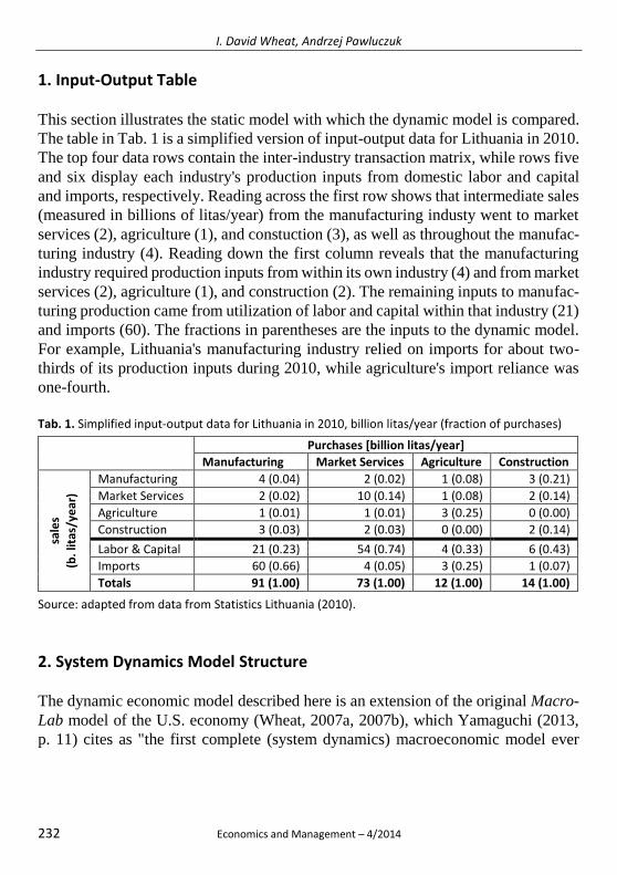
This section illustrates the static model with which the dynamic model is compared.

The table in Tab. 1 is a simplified version of input-output data for Lithuania in 2010.

The top four data rows contain the inter-industry transaction matrix, while rows five

and six display each industry's production inputs from domestic labor and capital

and imports, respectively. Reading across the first row shows that intermediate sales

(measured in billions of litas/year) from the manufacturing industy went to market

services (2), agriculture (1), and constuction (3), as well as throughout the manufac-

turing industry (4). Reading down the first column reveals that the manufacturing

industry required production inputs from within its own industry (4) and from market

services (2), agriculture (1), and construction (2). The remaining inputs to manufac-

turing production came from utilization of labor and capital within that industry (21)

and imports (60). The fractions in parentheses are the inputs to the dynamic model.

For example, Lithuania's manufacturing industry relied on imports for about two-

thirds of its production inputs during 2010, while agriculture's import reliance was

one-fourth.

Tab. 1. Simplified input-output data for Lithuania in 2010, billion litas/year (fraction of purchases)

Purchases [billion litas/year]

Manufacturing Market Services Agriculture Construction

sale

s

(b. l

itas

/ye

ar)

Manufacturing 4 (0.04) 2 (0.02) 1 (0.08) 3 (0.21)

Market Services 2 (0.02) 10 (0.14) 1 (0.08) 2 (0.14)

Agriculture 1 (0.01) 1 (0.01) 3 (0.25) 0 (0.00)

Construction 3 (0.03) 2 (0.03) 0 (0.00) 2 (0.14)

Labor & Capital 21 (0.23) 54 (0.74) 4 (0.33) 6 (0.43)

Imports 60 (0.66) 4 (0.05) 3 (0.25) 1 (0.07)

Totals 91 (1.00) 73 (1.00) 12 (1.00) 14 (1.00)

Source: adapted from data from Statistics Lithuania (2010).

2. System Dynamics Model Structure

The dynamic economic model described here is an extension of the original Macro-

Lab model of the U.S. economy (Wheat, 2007a, 2007b), which Yamaguchi (2013,

p. 11) cites as "the first complete (system dynamics) macroeconomic model ever



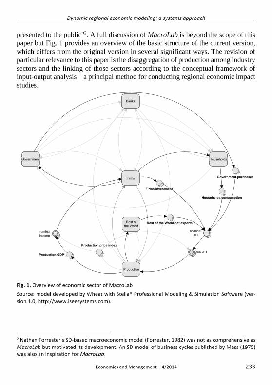
presented to the public"2. A full discussion of MacroLab is beyond the scope of this

paper but Fig. 1 provides an overview of the basic structure of the current version,

which differs from the original version in several significant ways. The revision of

particular relevance to this paper is the disaggregation of production among industry

sectors and the linking of those sectors according to the conceptual framework of

input-output analysis – a principal method for conducting regional economic impact

studies.

Fig. 1. Overview of economic sector of MacroLab

Source: model developed by Wheat with Stella® Professional Modeling & Simulation Software (ver-sion 1.0, http://www.iseesystems.com).

2 Nathan Forrester's SD-based macroeconomic model (Forrester, 1982) was not as comprehensive as MacroLab but motivated its development. An SD model of business cycles published by Mass (1975) was also an inspiration for MacroLab.



Five input-output submodels (agriculture, construction, manufacturing, market

services, and public services) are contained within the Production sector displayed

in the Fig. 1 diagram. The circular symbols with a multi-dimensional appearance are

arrayed variables that contain one or more vectors of information. The nominal in-

come variable, for example, contains information about income earned by factors of

production within the five industry categories of the model. The nominal AD (ag-

gregate demand) variable is a 4x5 array that contains information about four catego-

ries of aggregate demand, each with its own final demand for the five industry cate-

gories. A prefix on a variable identifies the submodel where its value is determined.

For example, the arrayed variable Production.price index, contains price indices for

the five industries and is calculated within the Production submodel. When nominal

AD is divided by Production.price index, the result is the arrayed variable real AD,

which is an input to the Production submodel.

Also visible in Fig. 1 are several feedback loops involving Production on the

"supply side" and the components of aggregate demand (consumption, investment,

government purchases, and net exports) on the "demand side" of the model economy.

Those loops are the transmission channels for what the input-output literature calls

the induced effect of a production stimulus; i.e., the feedback effect of additional

production on additional income and final demand. Within the Production sector,

a portion of each industry's production constitutes value added, and the total value

added is Production.GDP. Within the business Firms submodel, most of nominal

income is distributed to the Households and Governments submodels in the form of

wages and taxes; the rest is retained earnings. The dark arrows trace the return flow

of spending in the form of consumption, investment, government purchases, and net

exports3.

Within the Production submodel, there are five industry submodels, each linked

with one another. The four private sector submodels are identical in structure but

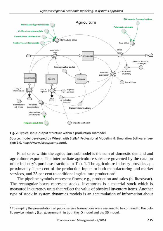
differ in their parameter values. Fig. 2, for example, displays the Agriculture sub-

model and its input-output structure4.

3 The light arrows indicate other linkages (e.g., transfer payments from Government to Households, bond sales from Government to Households, planned investment information from Production to Firms, and interest rate information from Banks to Production). 4 Equations for the Fig. 3 diagram are available upon request.



Fig. 2. Typical input-output structure within a production submodel

Source: model developed by Wheat with Stella® Professional Modeling & Simulation Software (ver-sion 1.0, http://www.iseesystems.com).

Final sales within the agriculture submodel is the sum of domestic demand and

agriculture exports. The intermediate agriculture sales are governed by the data on

other industry's purchase fractions in Tab. 1. The agriculture industry provides ap-

proximately 1 per cent of the production inputs to both manufacturing and market

services, and 25 per cent to additional agriculture production5.

The pipeline symbols represent flows; e.g., production and sales (b. litas/year).

The rectangular boxes represent stocks. Inventories is a material stock which is

measured in currency units that reflect the value of physical inventory items. Another

type of stock in system dynamics models is an accumulation of information about

5 To simplify the presentation, all public service transactions were assumed to be confined to the pub-lic service industry (i.e., government) in both the IO model and the SD model.



flows, such as Imports and Intermediate purchases in Fig. 2, measured in b. li-

tas/year. The Industry submodel contains the structure of labor, capital, productivity,

and prices within the agriculture industry. The output of that structure consists of

value added by the domestic agriculture industry, with the remainder sold to other

domestic industries. The agriculture production flow is the sum of the value of im-

ports, intermediate purchases, and value added by the domestic agriculture industry.

The production theory implicit in the Fig. 2 diagram is that the industry has

a norm for inventories called indicated inventory, which is a function of planned

inventory coverage (assumed to be about three months in this case) and sales (ini-

tially 12 b. litas/year, based on Tab. 1 data). When the model is initialized in equi-

librium for analytical purposes, initial production is also 12 b. litas/year until the

model is shocked. Based on data from the input-output matrix in Tab. 1, about one-

third of agriculture production will be generated by domestic labor and capital, about

one-fourth will be imported, and manufacturing and market services will each con-

tribute production inputs amounting to about eight per cent of agriculture's require-

ments. The indicated imports and indicated intermediate purchases will eventually

be realized, but not immediately; thus, the average adjustment time assumption of

six months for each.

The domestic industry production within the Industry submodel is based on

a Cobb-Douglas production function, and the stocks of labor and capital utilized de-

pend on wage rates, cost of capital, and the varying productivity of labor and capital.

Moreover, an industry-specific price index is calculated within the submodel, based

on demand pressures, cost pressures, and attainable mark-ups.

Information about the labor stock employed within the Industry submodel is

transmitted up to the Production submodel, where total employment is calculated for

the entire economy. When compared with the full labor force, an economy-wide

unemployment rate is calculated. The unemployment rate information is transmitted

back down to each Industry submodel, and the corresponding wage pressures influ-

ence the desired capital-labor ratio and the hiring rate for each industry. In a similar

manner, information about the capital stock and desired investment within each In-

dustry submodel is transmitted to the Firms submodel and, in conjunction with in-

terest rate information received from the Banks submodel, decisions about invest-

ment take into account retained earnings, dividends policy, and borrowing costs. The

cost of capital information feeds back to the Industry submodel and influences the

desired capital-labor ratio and the desired capital.



3. SD Model Behavior

The primary purpose of this paper is to discuss the structure of a system dynamics

model that integrates IO features while removing static constraints. In this section,

however, we take a brief look at the behavior of the model. Fig. 3 illustrates the

response to an export demand shock. Two hypothetical scenarios are tested, each

with the same sudden and permanent step increase in exports equal to 1 b. litas/year

(1 percent of GDP). In one scenario, the additional export demand is for manufac-

tured products; in the other scenario, the additional export demand is for agriculture

products. Measured behavior includes GDP and the unemployment rate.

Fig. 3. Simulated effects of two export demand shocks of equal magnitude

Source: simulation results with model developed by Wheat.

Both shocks have favourable impacts on the model economy, with GDP rising

and the unemployment rate falling. However, the "better" outcome occurs when the

export demand is directed towards agriculture rather than manufacturing. The expla-

nation stems from the input-output data: compared to the agriculture industry in this

illustrative model, the manufacturing industry is more reliant on imports for its in-

puts to production. Thus, relatively less of the increased export demand for manu-

facturing goods translates into value added production within that industry because

of the substantial "leakage" to pay for imported inputs. Without the IO structure, the

5,0

6,0

7,0

8,0

9,0

10,0

11,0

12,0

13,0

14,0

15,0

95

96

97

98

99

100

101

102

103

104

105

0 1 2 3 4 5 6 7 8 9 10

GDP Unemployment Rate

GDP after export shock to agriculture

GDP after export shock to manufacturing

UR after export shock to manufacturing

UR after export shock to agriculture

year



SD model would be incapable of revealing the differential effects of shocks identical

in magnitude but targeted at different industries.

Also of interest is a comparison of the behavior of the dynamic model with the

static IO model that relies on the same inter-industry production coefficients (in Tab.

1). First, we acknowledge that the static model also predicts that an import-depend-

ent manufacturing industry would contribute less to GDP than the agriculture indus-

try in the simulation experiment described above. The static model, however, is not

capable of suggesting the pattern of dynamic response for either industry. In Fig. 3,

the response patterns in both scenarios underscore the significance of delays that are

intrinsic to the dynamic model; the maximum impact takes nearly three years to be

realized. The impact is then sustained for about five years before stabilizing below

the maximum impact. A static outcome is timeless, by definition, but the implicit

future projection would be a flat line based on a static calculation of a constant mul-

tiplier effect – hardly a realistic scenario, but an inevitable one given the constraints

of a static model.

Conclusions

Let us now summarize how the dynamic model described in this paper eliminates or

relaxes key constraints inherent in traditional IO models. First, a fixed combination

of labor and capital is no longer assumed. As described above, labor and capital vary

within each industry submodel based on the target capital-labor ratio within that in-

dustry, a target that itself varies according to changes in productivity of labor and

capital and changes in wages and the cost of capital. Second, traditional IO models

not only assume fixed proportions of labor and capital, but also assume surplus pro-

ductive capacity that can fully respond to exogenous increases in demand. In the

dynamic model, however, labor and capital shortages can occur and can limit the

capacity of supply to respond to changing demand. Third, the changing costs, as well

as changes in demand pressures, cause prices to change in the model, thus eliminat-

ing another IO constraint. Moreover, the price changes are industry-specific, and the

economy-wide price index is a weighted-average of the industry price indices.

Fourth, the dynamic model contains a comprehensive set of feedback loops on the

demand side that channel household consumption, business investment, and govern-

ment spending in response to changes in income, in contrast to the static "induced"

demand effects calculated by treating households as a sector in an IO table.

A fifth constraint in IO models the assumption of a fixed technology that governs

the inter-industry inputs is not yet eliminated in our dynamic model. The technical



coefficients of the original IO table (Fig. 1) are used to allocate the source of inputs

to the overall production process in each industry submodel. Nevertheless, within

the industry submodels, most of the production is generated by labor and capital that

are endogenous to that industry. And that production process is not based on a static

production process, as noted above regarding the dynamics of labor, capital, produc-

tivity, and pricing. Thus, it is fair to say that the rigid production process assumption

in IO models is relaxed in our dynamic model. Future research will be aimed at dy-

namic modeling the influences on the coefficients in the IO table, with the goal of

eliminating the remaining constraint.

In addition, the next round of model development and evaluation will consider

how the SD-based model compares with SAM and CGE models. One important

question is whether the nonlinear feedback approach of SD treats income distribu-

tion and final demand in more satisfactory ways than SAM methods. We will also

investigate whether an SD model endogenizes prices and wages in more plausible

ways than the market-clearing approach of CGE models.

Notwithstanding the limitations of the current model, the approach described in

this paper indicates considerable potential for improving dynamic regional economic

modeling. The approach is based on integrating two methods – SD and IO – that use

complementary systemic lenses to view the operation of real-world economies. The

input-output framework enables SD models that would otherwise be too highly ag-

gregated to answer important questions about regional economic development and

policy design. The system dynamics framework enables IO analysts to embed their

methodology in a dynamic model and be relieved of constraints that raise questions

about the external validity of their analysis.

Literature

1. Armstrong H., Taylor J. (2000), Regional Economics and Policy, Blackwell, Oxford

2. Barlas Y. (2002), System Dynamics: Systemic Feedback Modeling for Policy Analysis,

in: Knowledge for Sustainable Development: An Insight Into the Encyclopedia of Life

Support Systems, UNESCO Publishing, Oxford

3. Braden C. (1981), System Dynamics and Input-Output Analysis, Proceedings of the

International Conference of the System Dynamics Society, Rensselaerville, New York

4. Ford A. (2010), Modeling the environment, 2nd ed., Island Press, Washington, DC

5. Forrester J.W. (1961), Industrial Dynamics, MIT Press, Cambridge, MA



6. Forrester N.B. (1982), A Dynamic Synthesis of Basic Macroeconomic Theory: Implica-

tions for Stabilization Policy Analysis, PhD Dissertation, Massachusetts Institute of

Technology, Cambridge, MA

7. Isard W., Azis I., Drennen M., Miller R., Saltzman S., Thoorbecke E. (1998), Methods

of Interregional and Regional Analysis, Ashgate, Aldershot

8. Krallman H. (1980), The Extended System Dynamics Method and its Tools, Kybernetes

9 (1), pp.15-31

9. McDonald G. (2005), Integrating Economics and Ecology: A Systems Approach to Sus-

tainability in the Auckland Region, PhD Dissertation, Massey University, Palmerston

North, New Zealand

10. Mass N.J. (1975), Economic Cycles: An Analysis of Underlying Causes, Wright-Allen

Press, Inc., Cambridge, MA

11. Shaffer R., Deller S., Marcouiller D. (2004), Community Economics: Linking Theory

and Practice, Blackwell, Oxford

12. Statistics Lithuania, Input-Output table at basic prices, domestic output and imports,

(2010), https://osp.stat.gov.lt/documents/10180/1923147/SanauduProdukcija_2010_13

1212.xlsx/fa76c823-aa54-48d2-bfa5-5da1ce988899 [01.12.2014]

13. Sterman J. (2000), Business Dynamics: Systems Thinking and Modeling for a Complex

World, Irwin/McGraw-Hill, Boston

14. Stimson R., Stough R., Roberts B. (2006), Regional Economic Development, Springer,

Berlin

15. Wheat I.D. (2007a), The Feedback Method: A System Dynamics Approach to Teaching

Macroeconomics, Ph.D. Dissertation, University of Bergen, Bergen, Norway, https://bo

ra.uib.no/handle/1956/2239 [01.12.2014]

16. Wheat I.D. (2007b), The Feedback Method of Teaching Macroeconomics: Is It Effec-

tive?, System Dynamics Review 23(4), 3pp. 91-413

17. Yamaguchi K. (2013), Money and Macroeconomic Dynamics: Accounting System Dy-

namics Approach, Japan Futures Research Center, Awaji Island, Japan

Dynamiczne modelowanie regionalnego rozwoju: podejście systemowe

Streszczenie

W artykule zaprezentowano sposób strukturalnego integrowania wewnętrznie generowa-nych właściwości statycznych modeli wejścia – wyjścia z ogólnym symulacyjnym modelem



dynamiki systemu. Celem takiej integracji jest dodanie nowej wartości w regionalnym mo-delowaniu ekonomicznym. Autorzy badają, w jaki sposób ograniczenia związane z tradycyj-nym modelem statycznym mogą zostać wyeliminowane i/lub pomniejszone w modelu dy-namicznym. Te ograniczenia wynikają z założeń przyjętej technologii, ustalonych relacji na-kładów pracy i kapitału, stałych cen i dodatkowych czynników produkcji. Wyjaśniamy, jak te ograniczenia mogą być zminimalizowane w modelu dynamiki systemu. Integracja dwóch metod pozwala na metodyczne rozgrupowanie modeli makroekonomicznych opartych na dynamice systemu oddziaływujących na siebie sektorów submodeli gospodarki, które uła-twiają badania wpływu gospodarczego regionów i mniejszych krajów. Okazuje się, że po-przez integrację, która eliminuje ograniczające założenia statyczne, ulega rozszerzeniu za-stosowanie i jakość analizy wejścia – wyjścia.

Słowa kluczowe

rozwój gospodarczy, wejście – wyjście, mnożnik, dynamika systemów

Author information

I. David Wheat

University of Bergen

Postboks 7806, N-5020 Bergen, Norway


Andrzej Pawluczuk

Bialystok University of Technology

Wiejska 45a, 15-351 Białystok, Poland


Dynamic regional economic modeling: a systems...

Documents

Transcript of Dynamic regional economic modeling: a systems...