MODELING DYNAMIC PROGRAMS
47
CHAPTER 5 MODELING DYNAMIC PROGRAMS Perhaps one of the most important skills to develop in approximate dynamic programming is the ability to write down a model of the problem. Everyone who wants to solve a linear program learns to write out min x c T x subject to Ax = b, x ≥ 0. This standard modeling framework allows people around the world to express their problem in a standard format. Stochastic, dynamic problems are much richer than a linear program, and require the ability to model the flow of information and complex system dynamics. Just the same, there is a standard framework for modeling dynamic programs. We provided a taste of this framework in chapter 2, but that chapter only hinted at the richness of the problem class. In chapters 2, 3 and 4, we used fairly standard notation, and have avoided discussing some important subtleties that arise in the modeling of stochastic, dynamic systems. We intentionally overlooked trying to define a state variable, which we have viewed as simply S t , where the set of states was given by the indexed set S = {1, 2,..., |S|}. We have avoided discussions of how to properly model time or more complex information processes. This style has facilitated introducing some basic ideas in dynamic programming, but would severely limit our ability to apply these methods to real problems. Approximate Dynamic Programming. By Warren B. Powell Copyright c 2010 John Wiley & Sons, Inc. 149
Transcript of MODELING DYNAMIC PROGRAMS

CHAPTER 5
MODELING DYNAMIC PROGRAMS
Perhaps one of the most important skills to develop in approximate dynamic programmingis the ability to write down a model of the problem. Everyone who wants to solve a linearprogram learns to write out
minxcTx
subject to
Ax = b,
x ≥ 0.
This standard modeling framework allows people around the world to express their problemin a standard format.
Stochastic, dynamic problems are much richer than a linear program, and require theability to model the flow of information and complex system dynamics. Just the same,there is a standard framework for modeling dynamic programs. We provided a taste of thisframework in chapter 2, but that chapter only hinted at the richness of the problem class.
In chapters 2, 3 and 4, we used fairly standard notation, and have avoided discussingsome important subtleties that arise in the modeling of stochastic, dynamic systems. Weintentionally overlooked trying to define a state variable, which we have viewed as simplySt, where the set of states was given by the indexed set S = 1, 2, . . . , |S|. We haveavoided discussions of how to properly model time or more complex information processes.This style has facilitated introducing some basic ideas in dynamic programming, but wouldseverely limit our ability to apply these methods to real problems.
Approximate Dynamic Programming. By Warren B. PowellCopyright c© 2010 John Wiley & Sons, Inc.
149

150 MODELING DYNAMIC PROGRAMS
The goal of this chapter is to describe a standard modeling framework for dynamicprograms, providing a vocabulary that will allow us to take on a much wider set ofapplications. Notation is not as critical for simple problems, as long as it is precise andconsistent. But what seems like benign notational decisions for a simple problem can causeunnecessary difficulties, possibly making the model completely intractable as problemsbecome more complex. Complex problems require considerable discipline in notationbecause they combine the details of the original physical problem with the challenge ofmodeling sequential information and decision processes. The modeling of time can beparticularly subtle. In addition to a desire to model problems accurately, we also need tobe able to understand and exploit the structure of the problem, which can become lost in asea of complex notation.
Good modeling begins with good notation. The choice of notation has to balancetraditional style with the needs of a particular problem class. Notation is easier to learn ifit is mnemonic (the letters look like what they mean) and compact (avoiding a profusionof symbols). Notation also helps to bridge communities. For example, it is common indynamic programming to refer to actions using “a” (where a is discrete); in control theory adecision (control) is “u” (which may be continuous). For high-dimensional problems, it isessential to draw on the field of mathematical programming, where decisions are typicallywritten as “x” and resource constraints are written in the standard form Ax = b. In thistext, many of our problems involve managing resources where we are trying to maximize orminimize an objective subject to constraints. For this reason, we adopt, as much as possible,the notation of math programming to help us bridge the fields of math programming anddynamic programming.
Sections 5.1 to 5.3 provide some foundational material. Section 5.1 begins by describingsome basic guidelines for notational style. Section 5.2 addresses the critical question ofmodeling time, and section 5.3 provides notation for modeling resources that we will usethroughout the remainder of the volume.
The general framework for modeling a dynamic program is covered in sections 5.4 to5.8. There are five elements to a dynamic program, consisting of the following:
1) State variables - These describe what we need to know at a point in time (section 5.4).
2) Decision variables - These are the variables we control. Choosing these variables (“mak-ing decisions”) represents the central challenge of dynamic programming (section5.5).
3) Exogenous information processes - These variables describe information that arrives tous exogenously, representing the sources of randomness (section 5.6).
4) Transition function - This is the function that describes how the state evolves from onepoint in time to another (section 5.7).
5) Objective function - We are either trying to maximize a contribution function (profits,revenues, rewards, utility) or minimize a cost function. This function describes howwell we are doing at a point in time (section 5.8).
This chapter describes modeling in considerable depth, and as a result it is quite long. Anumber of sections are marked with a ‘*’, indicating that these can be skipped on a firstread. There is a single section marked with a ‘**’ which, as with all sections markedthis way, is material designed for readers with more advanced training in probability andstochastic processes.

NOTATIONAL STYLE 151
5.1 NOTATIONAL STYLE
Notation is a language: the simpler the language, the easier it is to understand the problem.As a start, it is useful to adopt notational conventions to simplify the style of our presentation.For this reason, we adopt the following notational conventions:
Variables - Variables are always a single letter. We would never use, for example, CH for“holding cost.”
Modeling time - We always use t to represent a point in time, while we use τ to representan interval over time. When we need to represent different points in time, we mightuse t, t′, t, tmax, and so on.
Indexing vectors - Vectors are almost always indexed in the subscript, as in xij . Since weuse discrete time models throughout, an activity at time t can be viewed as an elementof a vector. When there are multiple indices, they should be ordered from outside inthe general order over which they might be summed (think of the outermost indexas the most detailed information). So, if xtij is the flow from i to j at time t withcost ctij , we might sum up the total cost using
∑t
∑i
∑j ctijxtij . Dropping one or
more indices creates a vector over the elements of the missing indices to the right.So, xt = (xtij)∀i,∀j is the vector of all flows occurring at time t. If we write xti,this would be the vector of flows out of i at time t to all destinations j. Time, whenpresent, is always the innermost index.
Indexing time - If we are modeling activities in discrete time, then t is an index andshould be put in the subscript. So xt would be an activity at time t, with the vectorx = (x1, x2, . . . , xt, . . . , xT ) giving us all the activities over time. When modelingproblems in continuous time, it is more common to write t as an argument, as in x(t).xt is notationally more compact (try writing a complex equation full of variableswritten as x(t) instead of xt).
Flavors of variables - It is often the case that we need to indicate different flavors ofvariables, such as holding costs and order costs. These are always indicated assuperscripts, where we might write ch or chold as the holding cost. Note that whilevariables must be a single letter, superscripts may be words (although this should beused sparingly). We think of a variable like “ch” as a single piece of notation. It isbetter to write ch as the holding cost and cp as the purchasing cost than to use h asthe holding cost and p as the purchasing cost (the first approach uses a single letterc for cost, while the second approach uses up two letters - the roman alphabet is ascarce resource). Other ways of indicating flavors is hats (x), bars (x), tildes (x) andprimes (x′).
Iteration counters - We place iteration counters in the superscript, and we primarily usen as our iteration counter. So, xn is our activity at iteration n. If we are using adescriptive superscript, we might write xh,n to represent xh at iterationn. Sometimesalgorithms require inner and outer iterations. In this case, we use n to index the outeriteration and m for the inner iteration. While this will prove to be the most naturalway to index iterations, there is potential for confusion where it may not be clear ifthe superscript n is an index (as we view it) or raising a variable to the nth power. Wemake one notable exception to our policy of indexing iterations in the superscript.In approximate dynamic programming, we make wide use of a parameter known as

152 MODELING DYNAMIC PROGRAMS
a stepsize α where 0 ≤ α ≤ 1. We often make the stepsize vary with the iterations.However, writing αn looks too much like raising the stepsize to the power of n.Instead, we write αn to indicate the stepsize in iteration n. This is our only exceptionto this rule.
Sets are represented using capital letters in a calligraphic font, such as X ,F or I. Wegenerally use the lowercase roman letter as an element of a set, as in x ∈ X or i ∈ I.
Exogenous information - Information that first becomes available (from outside the sys-tem) at time t is denoted using hats, for example, Dt or pt. Our only exception tothis rule is Wt which is our generic notation for exogenous information (since Wt
always refers to exogenous information, we do not use a hat).
Statistics - Statistics computed using exogenous information are generally indicated usingbars, for example xt or V t. Since these are functions of random variables, they arealso random.
Index variables - Throughout, i, j, k, l,m and n are always scalar indices.
Of course, there are exceptions to every rule. It is extremely common in the transportationliterature to model the flow of a type of resource (called a commodity and indexed by k)from i to j using xkij . Following our convention, this should be written xkij . Authors needto strike a balance between a standard notational style and existing conventions.
5.2 MODELING TIME
A survey of the literature reveals different styles toward modeling time. When usingdiscrete time, some authors start at 1 while others start at zero. When solving finite horizonproblems, it is popular to index time by the number of time periods remaining, rather thanelapsed time. Some authors index a variable, say St, as being a function of information upthrough t − 1, while others assume it includes information up through time t. t may beused to represent when a physical event actually happens, or when we first know about aphysical event.
The confusion over modeling time arises in large part because there are two processesthat we have to capture: the flow of information, and the flow of physical and financialresources. There are many applications of dynamic programming to deterministic problemswhere the flow of information does not exist (everything is known in advance). Similarly,there are many models where the arrival of the information about a physical resource, andwhen the information takes effect in the physical system, are the same. For example, thetime at which a customer physically arrives to a queue is often modeled as being the sameas when the information about the customer first arrives. Similarly, we often assume thatwe can sell a resource at a market price as soon as the price becomes known.
There is a rich collection of problems where the information process and physicalprocess are different. A buyer may purchase an option now (an information event) tobuy a commodity in the future (the physical event). Customers may call an airline (theinformation event) to fly on a future flight (the physical event). An electric power companyhas to purchase equipment now to be used one or two years in the future. All of theseproblems represent examples of lagged information processes and force us to explicitlymodel the informational and physical events (see section 2.2.7 for an illustration).

MODELING TIME 153
1t = 2t = 3t = 4t =
0t = 1t = 2t = 3t = 4t =
5.1a: Information processes
1t = 2t = 3t =0t =
1t = 2t = 3t =0t =
5.1b: Physical processes
Figure 5.1 Relationship between discrete and continuous time for information processes (5.1a)and physical processes (5.1b).
Notation can easily become confused when an author starts by writing down a determin-istic model of a physical process, and then adds uncertainty. The problem arises becausethe proper convention for modeling time for information processes is different than whatshould be used for physical processes.
We begin by establishing the relationship between discrete and continuous time. Allof the models in this book assume that decisions are made in discrete time (sometimesreferred to as decision epochs). However, the flow of information, and many of the physicalprocesses being modeled, are best viewed in continuous time. A common error is to assumethat when you model a dynamic program in discrete time then all events (information eventsand physical events) are also occurring in discrete time (in some applications, this is thecase). Throughout this volume, decisions are made in discrete time, while all other activitiesoccur in continuous time.
The relationship of our discrete time approximation to the real flow of information andphysical resources is depicted in figure 5.1. Above the line, “t” refers to a time intervalwhile below the line, “t” refers to a point in time. When we are modeling information,time t = 0 is special; it represents “here and now” with the information that is availableat the moment. The discrete time t refers to the time interval from t − 1 to t (illustratedin figure 5.1a). This means that the first new information arrives during time interval 1.This notational style means that any variable indexed by t, say St or xt, is assumed to haveaccess to the information that arrived up to time t, which means up through time interval t.This property will dramatically simplify our notation in the future. For example, assumethat ft is our forecast of the demand for electricity. If Dt is the observed demand duringtime interval t, we would write our updating equation for the forecast using
ft = (1− α)ft−1 + αDt. (5.1)
We refer to this form as the informational representation. Note that the forecast ft iswritten as a function of the information that became available during time interval t.
When we are modeling a physical process, it is more natural to adopt a differentconvention (illustrated in figure 5.1b): discrete time t refers to the time interval betweent and t + 1. This convention arises because it is most natural in deterministic models to

154 MODELING DYNAMIC PROGRAMS
use time to represent when something is happening or when a resource can be used. Forexample, let Rt be our cash on hand that we can use during day t (implicitly, this meansthat we are measuring it at the beginning of the day). Let Dt be the demand for cash duringthe day, and let xt represent additional cash that we have decided to add to our balance (tobe used during day t). We can model our cash on hand using
Rt+1 = Rt + xt − Dt. (5.2)
We refer to this form as the actionable representation. Note that the left-hand side isindexed by t + 1, while all the quantities on the right-hand side are indexed by t. Thisequation makes perfect sense when we interpret time t to represent when a quantity can beused. For example, many authors would write our forecasting equation (5.1) as
ft+1 = (1− α)ft + αDt. (5.3)
This equation is correct if we interpret ft as the forecast of the demand that will happen intime interval t.
A review of the literature quickly reveals that both modeling conventions are widelyused. It is important to be aware of the two conventions and how to interpret them. Wehandle the modeling of informational and physical processes by using two time indices, aform that we refer to as the “(t, t′)” notation. For example,
Dtt′ = The demands that first become known during time interval t to be servedduring time interval t′.
ftt′ = The forecast for activities during time interval t′ made using the informationavailable up through time t.
Rtt′ = The resources on hand at time t that cannot be used until time t′.xtt′ = The decision to purchase futures at time t to be exercised during time interval
t′.
For each variable, t indexes the information content (literally, when the variable is measuredor computed), while t′ represents the time at which the activity takes place. Each of thesevariables can be written as vectors, such as
Dt = (Dtt′)t′≥t,
ft = (ftt′)t′≥t,
xt = (xtt′)t′≥t,
Rt = (Rtt′)t′≥t.
Note that these vectors are now written in terms of the information content. For stochasticproblems, this style is the easiest and most natural. If we were modeling a deterministicproblem, we would drop the first index “t” and model the entire problem in terms of thesecond index “t′.”
Each one of these quantities is computed at the end of time interval t (that is, with theinformation up through time interval t) and represents a quantity that can be used at timet′ in the future. We could adopt the convention that the first time index uses the indexingsystem illustrated in figure 5.1a, while the second time index uses the system in figure 5.1b.While this convention would allow us to easily move from a natural deterministic model toa natural stochastic model, we suspect most people will struggle with an indexing systemwhere time interval t in the information process refers to time interval t− 1 in the physical

MODELING RESOURCES 155
process. Instead, we adopt the convention to model information in the most natural way,and live with the fact that product arriving at time t can only be used during time intervalt+ 1.
Using this convention it is instructive to interpret the special case where t = t′. Dtt issimply demands that arrive during time interval t, where we first learn of them when theyarrive. ftt makes no sense, because we would never forecast activities during time intervalt after we have this information. Rtt represents resources that we know about during timeinterval t and which can be used during time interval t. Finally, xtt is a decision to purchaseresources to be used during time interval t given the information that arrived during timeinterval t. In financial circles, this is referred to as purchasing on the spot market.
The most difficult notational decision arises when first starting to work on a problem.It is natural at this stage to simplify the problem (often, the problem appears simple) andthen choose notation that seems simple and natural. If the problem is deterministic andyou are quite sure that you will never solve a stochastic version of the problem, then theactionable representation (figure 5.1b) and equation (5.2) is going to be the most natural.Otherwise, it is best to choose the informational format. If you do not have to deal withlagged information processes (e.g., ordering at time t to be used at some time t′ in thefuture) you should be able to get by with a single time index, but you need to rememberthat xt may mean purchasing product to be used during time interval t+ 1.
Care has to be used when taking expectations of functions. Consider what happens whenwe want to know the expected costs to satisfy customer demands Dt that arose during timeinterval t given the decision xt−1 we made at time t − 1. We would have to computeECt(xt−1, Dt), where the expectation is over the random variable Dt. The function thatresults from taking the expectation is now a function of information up through time t− 1.Thus, we might use the notation
Ct−1(xt−1) = ECt(xt−1, Dt).
This can take a little getting used to. The costs are incurred during time interval t, but nowwe are indexing the function with time t − 1. The problem is that if we use a single timeindex, we are not capturing when the activity is actually happening. An alternative is toswitch to a double time index, as in
Ct−1,t(xt−1) = ECt(xt−1, Dt),
where Ct−1,t(xt−1) is the expected costs that will be incurred during time interval t usingthe information known at time t− 1.
5.3 MODELING RESOURCES
There is a vast range of problems that can be broadly described in terms of managing“resources.” Resources can be equipment, people, money, robots or even games such asbackgammon or chess. Depending on the setting, we might use the term asset (financialapplications, expensive equipment) or entity (managing a robot, playing a board game). Itis very common to start with fairly simple models of these problems, but the challenge isto solve complex problems.
There are four important problem classes that we consider in this volume, each offeringunique computational challenges. These can be described along two dimensions: thenumber of resources or entities being managed, and the complexity of the attributes of each

156 MODELING DYNAMIC PROGRAMS
resource or entity. We may be managing a single entity (a robot, an aircraft, an electricalpower plant) or multiple entities (a fleet of aircraft, trucks or locomotives, funds in differentasset classes, groups of people). The attributes of each entity or resource may be simple(the truck may be described by its location, the money by the asset class into which it hasbeen invested) or complex (all the characteristics of an aircraft or pilot).
The computational implications of each problem class can be quite different. Notsurprisingly, different communities tend to focus on specific problem classes, making itpossible for people to make the connection between mathematical notation (which can beelegant but vague) and the characteristics of a problem. Problems involving a single, simpleentity can usually be solved using the classical techniques of Markov decision processes(chapter 3), although even here some problems can be difficult. The artificial intelligencecommunity often works on problems involving a single, complex entity (games such asConnect-4 and backgammon, moving a robot arm or flying an aircraft). The operationsresearch community has major subcommunities working on problems that involve multiple,simple entities (multicommodity flow problems, inventory problems), while portions of thesimulation community and math programming community (for deterministic problems)will work on applications with multiple, complex entities.
In this section, we describe notation that allows us to evolve from simple to complexproblems in a natural way. Our goal is to develop mathematical notation that does a betterjob of capturing which problem class we are working on.
5.3.1 Modeling a single, discrete resource
Many problems in dynamic programming involve managing a single resource such as flyingan aircraft, planning a path through a network, or planning a game of chess or backgammon.These problems are distinctly different than those involving the management of fleets ofvehicles, inventories of blood or groups of people. For this reason, we adopt specificnotation for the single entity problem.
If we are managing a single, discrete resource, we find it useful to introduce specificnotation to model the attributes of the resource. For this purpose, we use
rt = The attribute vector of the resource at time t= (rt1, rt2, . . . , rtN ),
R = Set of all possible attribute vectors.
Attributes might be discrete (0, 1, 2, . . . ), continuous (0 ≤ ri ≤ 1) or categorical (ri = red).We typically assume that the number of dimensions of rt is not too large. For example,if we are modeling the flow of product through a supply chain, the attribute vector mightconsist of the product type and location. If we are playing chess, the attribute vector wouldhave 64 dimensions (the piece on each square of the board).
MODELING RESOURCES 157
5.3.2 Modeling multiple resources
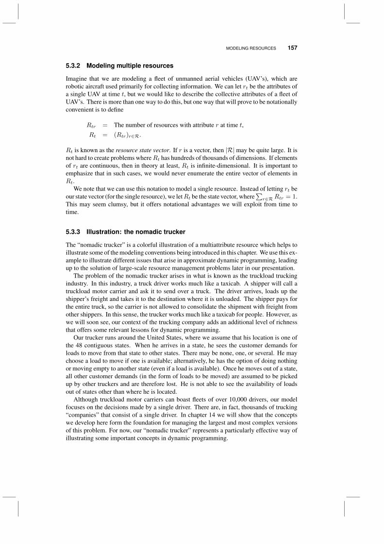
Imagine that we are modeling a fleet of unmanned aerial vehicles (UAV’s), which arerobotic aircraft used primarily for collecting information. We can let rt be the attributes ofa single UAV at time t, but we would like to describe the collective attributes of a fleet ofUAV’s. There is more than one way to do this, but one way that will prove to be notationallyconvenient is to define
Rtr = The number of resources with attribute r at time t,Rt = (Rtr)r∈R.
Rt is known as the resource state vector. If r is a vector, then |R| may be quite large. It isnot hard to create problems whereRt has hundreds of thousands of dimensions. If elementsof rt are continuous, then in theory at least, Rt is infinite-dimensional. It is important toemphasize that in such cases, we would never enumerate the entire vector of elements inRt.
We note that we can use this notation to model a single resource. Instead of letting rt beour state vector (for the single resource), we letRt be the state vector, where
∑r∈RRtr = 1.
This may seem clumsy, but it offers notational advantages we will exploit from time totime.
5.3.3 Illustration: the nomadic trucker
The “nomadic trucker” is a colorful illustration of a multiattribute resource which helps toillustrate some of the modeling conventions being introduced in this chapter. We use this ex-ample to illustrate different issues that arise in approximate dynamic programming, leadingup to the solution of large-scale resource management problems later in our presentation.
The problem of the nomadic trucker arises in what is known as the truckload truckingindustry. In this industry, a truck driver works much like a taxicab. A shipper will call atruckload motor carrier and ask it to send over a truck. The driver arrives, loads up theshipper’s freight and takes it to the destination where it is unloaded. The shipper pays forthe entire truck, so the carrier is not allowed to consolidate the shipment with freight fromother shippers. In this sense, the trucker works much like a taxicab for people. However, aswe will soon see, our context of the trucking company adds an additional level of richnessthat offers some relevant lessons for dynamic programming.
Our trucker runs around the United States, where we assume that his location is one ofthe 48 contiguous states. When he arrives in a state, he sees the customer demands forloads to move from that state to other states. There may be none, one, or several. He maychoose a load to move if one is available; alternatively, he has the option of doing nothingor moving empty to another state (even if a load is available). Once he moves out of a state,all other customer demands (in the form of loads to be moved) are assumed to be pickedup by other truckers and are therefore lost. He is not able to see the availability of loadsout of states other than where he is located.
Although truckload motor carriers can boast fleets of over 10,000 drivers, our modelfocuses on the decisions made by a single driver. There are, in fact, thousands of trucking“companies” that consist of a single driver. In chapter 14 we will show that the conceptswe develop here form the foundation for managing the largest and most complex versionsof this problem. For now, our “nomadic trucker” represents a particularly effective way ofillustrating some important concepts in dynamic programming.

158 MODELING DYNAMIC PROGRAMS
A basic modelThe simplest model of our nomadic trucker assumes that his only attribute is his location,which we assume has to be one of the 48 contiguous states. We let
I = The set of “states” (locations) at which the driver can be located.
We use i and j to index elements of I. His attribute vector then consists of
r = i.
In addition to the attributes of the driver, we also have to capture the attributes of the loadsthat are available to be moved. For our basic model, loads are characterized only by wherethey are going. Let
b = The vector of characteristics of a load
=
(b1b2
)=
(The origin of the load.The destination of the load.
).
We let R be the set of all possible values of the driver attribute vector r, and we let B bethe set of all possible load attribute vectors b.
A more realistic modelWe need a richer set of attributes to capture some of the realism of an actual truck driver.To begin, we need to capture the fact that at a point in time, a driver may be in the processof moving from one location to another. If this is the case, we represent the attribute vectoras the attribute that we expect when the driver arrives at the destination (which is the nextpoint at which we can make a decision). In this case, we have to include as an attribute thetime at which we expect the driver to arrive.
Second, we introduce the dimension that the equipment may fail, requiring some levelof repair. A failure can introduce additional delays before the driver is available.
A third important dimension covers the rules that limit how much a driver can be on theroad. In the United States, drivers are governed by a set of rules set by the Department ofTransportation (“DOT”). There are three basic limits: the amount a driver can be behindthe wheel in one shift, the amount of time a driver can be “on duty” in one shift (includestime waiting), and the amount of time that a driver can be on duty over any contiguouseight-day period. As of this writing, these rules are as follows: a driver can drive at most 11hours at a stretch, he may be on duty for at most 14 continuous hours (there are exceptionsto this rule), and the driver can work at most 70 hours in any eight-day period. The lastclock is reset if the driver is off-duty for 34 successive hours during any stretch (known asthe “34-hour reset”).
A final dimension involves getting a driver home. In truckload trucking, drivers may beaway from home for several weeks at a time. Companies work to assign drivers that getthem home in a reasonable amount of time.

THE STATES OF OUR SYSTEM 159
If we include these additional dimensions, our attribute vector grows to
rt =
r1
r2
r3
r4
r5
r6
r7
r8
=
The current or future location of the driver.The time at which the driver is expected to arrive at his future location.The maintenance status of the equipment.The number of hours a driver has been behind the wheel during hiscurrent shift.The number of hours a driver has been on-duty during his current shift.
An eight-element vector giving the number of hours the driver was onduty over each of the previous eight days.The driver’s home domicile.
The number of days a driver has been away from home.
.
We note that element r6 is actually a vector that holds the number of hours the driver wason duty during each calendar day over the last eight days.
A single attribute such as location (including the driver’s domicile) might have 100outcomes, or over 1,000. The number of hours a driver has been on the road might bemeasured to the nearest hour, while the number of days away from home can be as large as30 (in rare cases). Needless to say, the number of potential attribute vectors is extremelylarge.
5.4 THE STATES OF OUR SYSTEM
The most important quantity in a dynamic program is the state variable. The state variablecaptures what we need to know, but just as important it is the variable around which weconstruct value function approximations. Success in developing a good approximationstrategy depends on a deep understanding of what is important in a state variable to capturethe future behavior of a system.
5.4.1 Defining the state variable
Surprisingly, other presentations of dynamic programming spend little time defining a statevariable. Bellman’s seminal text [Bellman (1957), p. 81] says “... we have a physical systemcharacterized at any stage by a small set of parameters, the state variables.” In a much moremodern treatment, Puterman first introduces a state variable by saying [Puterman (2005),p. 18] “At each decision epoch, the system occupies a state.” In both cases, the italics arein the original manuscript, indicating that the term “state” is being introduced. In effect,both authors are saying that given a system, the state variable will be apparent from thecontext.
Interestingly, different communities appear to interpret state variables in slightly differentways. We adopt an interpretation that is fairly common in the control theory community,but offer a definition that appears to be somewhat tighter than what typically appears in theliterature. We suggest the following definition:
Definition 5.4.1 A state variable is the minimally dimensioned function of history that isnecessary and sufficient to compute the decision function, the transition function, and thecontribution function.
Later in the chapter, we discuss the decision function (section 5.5), the transition function(section 5.7), and the objective function (section 5.8). In plain English, a state variable is

160 MODELING DYNAMIC PROGRAMS
all the information you need to know (at time t) to model the system from time t onward.Initially, it is easiest to think of the state variable in terms of the physical state of the system(the status of the pilot, the amount of money in our bank account), but ultimately it isnecessary to think of it as the “state of knowledge.”
This definition provides a very quick test of the validity of a state variable. If there isa piece of data in either the decision function, the transition function, or the contributionfunction which is not in the state variable, then we do not have a complete state variable.Similarly, if there is information in the state variable that is never needed in any of thesethree functions, then we can drop it and still have a valid state variable.
We use the term “minimally dimensioned function” so that our state variable is ascompact as possible. For example, we could argue that we need the entire history ofevents up to time t to model future dynamics. But this is not practical. As we start doingcomputational work, we are going to want St to be as compact as possible. Furthermore,there are many problems where we simply do not need to know the entire history. It mightbe enough to know the status of all our resources at time t (the resource variable Rt). Butthere are examples where this is not enough.
Assume, for example, that we need to use our history to forecast the price of a stock.Our history of prices is given by (p1, p2, . . . , pt). If we use a simple exponential smoothingmodel, our estimate of the mean price pt can be computed using
pt = (1− α)pt−1 + αpt,
where α is a stepsize satisfying 0 ≤ α ≤ 1. With this forecasting mechanism, we do notneed to retain the history of prices, but rather only the latest estimate pt. As a result, pt iscalled a sufficient statistic, which is a statistic that captures all relevant information neededto compute any additional statistics from new information. A state variable, according toour definition, is always a sufficient statistic.
Consider what happens when we switch from exponential smoothing to an N -periodmoving average. Our forecast of future prices is now given by
pt =1
N
N−1∑τ=0
pt−τ .
Now, we have to retain the N -period rolling set of prices (pt, pt−1, . . . , pt−N+1) in orderto compute the price estimate in the next time period. With exponential smoothing, wecould write
St = pt.
If we use the moving average, our state variable would be
St = (pt, pt−1, . . . , pt−N+1). (5.4)
Many authors say that if we use the moving average model, we no longer have a properstate variable. Rather, we would have an example of a “history-dependent process” wherethe state variable needs to be augmented with history. Using our definition of a statevariable, the concept of a history-dependent process has no meaning. The state variableis simply the minimal information required to capture what is needed to model futuredynamics. Needless to say, having to explicitly retain history, as we did with the movingaverage model, produces a much larger state variable than the exponential smoothing model.

THE STATES OF OUR SYSTEM 161
5.4.2 The three states of our system
To set up our discussion, assume that we are interested in solving a relatively complexresource management problem, one that involves multiple (possibly many) different typesof resources which can be modified in various ways (changing their attributes). For such aproblem, it is necessary to work with three types of states:
The physical state - This is a snapshot of the status of the physical resources we aremanaging and their attributes. This might include the amount of water in a reservoir,the price of a stock or the location of a sensor on a network.
The information state - This encompasses the physical state as well as any other infor-mation we need to make a decision, compute the transition or compute the objectivefunction.
The belief/knowledge state - If the information state is what we know, the belief state(also known as the knowledge state) captures how well we know it. This conceptis largely absent from most dynamic programs, but arises in the setting of partiallyobservable processes (when we cannot observe a portion of the state variable).
There are many problems in dynamic programming that involve the management of asingle resource or entity (or asset - the best terminology depends on the context), suchas using a computer to play backgammon, routing a single aircraft, controlling a powerplant, or selling an asset. There is nothing wrong with letting St be the state of this entity.When we are managing multiple entities (which often puts us in the domain of “resourcemanagement”), it is often useful to distinguish between the state of a single entity, whichwe represent as rt, versus the state of all the entities, which we represent as Rt.
We can use St to be the state of a single resource (if this is all we are managing), orlet St = Rt be the state of all the resources we are managing. There are many problemswhere the state of the system consists only of rt or Rt. We suggest using St as a genericstate variable when it is not important to be specific, but it must be used when we maywish to include other forms of information. For example, we might be managing resources(consumer products, equipment, people) to serve customer demands Dt that become knownat time t. If Rt describes the state of the resources we are managing, our state variablewould consist of St = (Rt, Dt), where Dt represents additional information we need tosolve the problem.
Alternatively, other information might include estimates of parameters of the system(costs, speeds, times, prices). To represent this, let
θt = A vector of estimates of different problem parameters at time t.θt = New information about problem parameters that arrive during
time interval t.
We can think of θt as the state of our information about different problem parameters attime t. We can now write a more general form of our state variable as:
St = The information state at time t= (Rt, θt).
In chapter 12, we will show that it is important to include not just the point estimate θt,but the entire distribution (or the parameters needed to characterize the distribution, suchas the variance).
162 MODELING DYNAMIC PROGRAMS
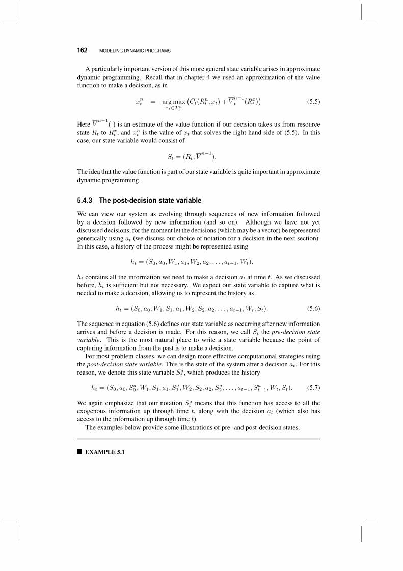
A particularly important version of this more general state variable arises in approximatedynamic programming. Recall that in chapter 4 we used an approximation of the valuefunction to make a decision, as in
xnt = arg maxxt∈Xnt
(Ct(R
nt , xt) + V
n−1
t (Rxt ))
(5.5)
Here Vn−1
(·) is an estimate of the value function if our decision takes us from resourcestate Rt to Rxt , and xnt is the value of xt that solves the right-hand side of (5.5). In thiscase, our state variable would consist of
St = (Rt, Vn−1
).
The idea that the value function is part of our state variable is quite important in approximatedynamic programming.
5.4.3 The post-decision state variable
We can view our system as evolving through sequences of new information followedby a decision followed by new information (and so on). Although we have not yetdiscussed decisions, for the moment let the decisions (which may be a vector) be representedgenerically using at (we discuss our choice of notation for a decision in the next section).In this case, a history of the process might be represented using
ht = (S0, a0,W1, a1,W2, a2, . . . , at−1,Wt).
ht contains all the information we need to make a decision at at time t. As we discussedbefore, ht is sufficient but not necessary. We expect our state variable to capture what isneeded to make a decision, allowing us to represent the history as
ht = (S0, a0,W1, S1, a1,W2, S2, a2, . . . , at−1,Wt, St). (5.6)
The sequence in equation (5.6) defines our state variable as occurring after new informationarrives and before a decision is made. For this reason, we call St the pre-decision statevariable. This is the most natural place to write a state variable because the point ofcapturing information from the past is to make a decision.
For most problem classes, we can design more effective computational strategies usingthe post-decision state variable. This is the state of the system after a decision at. For thisreason, we denote this state variable Sat , which produces the history
ht = (S0, a0, Sa0 ,W1, S1, a1, S
a1 ,W2, S2, a2, S
a2 , . . . , at−1, S
at−1,Wt, St). (5.7)
We again emphasize that our notation Sat means that this function has access to all theexogenous information up through time t, along with the decision at (which also hasaccess to the information up through time t).
The examples below provide some illustrations of pre- and post-decision states.
EXAMPLE 5.1

THE STATES OF OUR SYSTEM 163
A traveler is driving through a network, where the travel time on each link of thenetwork is random. As she arrives at node i, she is allowed to see the travel times oneach of the links out of node i, which we represent by τi = (τij)j . As she arrives atnode i, her pre-decision state is St = (i, τi). Assume she decides to move from i to k.Her post-decision state is Sat = (k) (note that she is still at node i; the post-decisionstate captures the fact that she will next be at node k, and we no longer have to includethe travel times on the links out of node i).
EXAMPLE 5.2
The nomadic trucker revisited. Let Rtr = 1 if the trucker has attribute vector r attime t and 0 otherwise. Now let Dtb be the number of customer demands (loads offreight) of type b available to be moved at time t. The pre-decision state variablefor the trucker is St = (Rt, Dt), which tells us the state of the trucker and thedemands available to be moved. Assume that once the trucker makes a decision, allthe unserved demands in Dt are lost, and new demands become available at timet + 1. The post-decision state variable is given by Sat = Rat where Ratr = 1 if thetrucker has attribute vector r after a decision has been made.
EXAMPLE 5.3
Imagine playing backgammon where Rti is the number of your pieces on the ith
“point” on the backgammon board (there are 24 points on a board). The transitionfrom St to St+1 depends on the player’s decision at, the play of the opposing player,and the next roll of the dice. The post-decision state variable is simply the state ofthe board after a player moves but before his opponent has moved.
The importance of the post-decision state variable, and how to use it, depends on theproblem at hand. We saw in chapter 4 that the post-decision state variable allowed us tomake decisions without having to compute the expectation within the max or min operator.Later we will see that this allows us to solve some very large scale problems.
There are three ways of finding a post-decision state variable:
Decomposing decisions and information There are many problems where we cancreate functions SM,a(·) and SM,W (·) from which we can compute
Sat = SM,a(St, at), (5.8)St+1 = SM,W (Sat ,Wt+1). (5.9)
The structure of these functions is highly problem-dependent. However, there are some-times significant computational benefits, primarily when we face the problem of approx-imating the value function. Recall that the state variable captures all the information weneed to make a decision, compute the transition function, and compute the contributionfunction. Sat only has to carry the information needed to compute the transition function.For some applications, Sat has the same dimensionality as St, but in many settings, Sat isdramatically simpler than St, simplifying the problem of approximating the value function.

164 MODELING DYNAMIC PROGRAMS
Pre-decision State-action Post-decisionSt (St, at) (Sat )
⎛⎜⎜⎜⎝
⎞⎟⎟⎟⎠
5.2a 5.2b 5.2c
Figure 5.2 Pre-decision state, augmented state-action, and post-decision state for tic-tac-toe.
State-action pairs A very generic way of representing a post-decision state is to simplywrite
Sat = (St, at).
Figure 5.2 provides a nice illustration using our tic-tac-toe example. Figure 5.2a shows atic-tac-toe board just before player O makes his move. Figure 5.2b shows the augmentedstate-action pair, where the decision (O decides to place his move in the upper right handcorner) is distinct from the state. Finally, figure 5.2c shows the post-decision state. Forthis example, the pre- and post-decision state spaces are the same, while the augmentedstate-action pair is nine times larger.
The augmented state (St, at) is closely related to the post-decision state Sat (not surpris-ing, since we can compute Sat deterministically from St and at). But computationally, thedifference is significant. If S is the set of possible values of St, andA is the set of possiblevalues of at, then our augmented state space has size |S| × |A|, which is obviously muchlarger.
The augmented state variable is used in a popular class of algorithms known as Q-learning (introduced in chapter 6), where the challenge is to statistically estimateQ-factorswhich give the value of being in state St and taking action at. The Q-factors are writtenQ(St, at), in contrast with value functions Vt(St) which provide the value of being in astate. This allows us to directly find the best action by solving minaQ(St, at). This isthe essence of Q-learning, but the price of this algorithmic step is that we have to estimateQ(St, at) for each St and at. It is not possible to determine at by optimizing a function ofSat alone, since we generally cannot determine which action at brought us to Sat .
The post-decision as a point estimate Assume that we have a problem wherewe can compute a point estimate of future information. Let Wt,t+1 be a point estimate,computed at time t, of the outcome of Wt+1. If Wt+1 is a numerical quantity, we mightuse Wt,t+1 = E(Wt+1|St) or Wt,t+1 = 0. Wt+1 might be a discrete outcome such asthe number of equipment failures. It may not make sense to use an expectation (we mayhave problems working with 0.10 failures), so in this settingWt+1 might be the most likelyoutcome. Finally, we might simply assume that Wt+1 is empty (a form of “null” field).For example, a taxi picking up a customer may not know the destination of the customerbefore the customer gets in the cab. In this case, if Wt+1 represents the destination, wemight use Wt,t+1 = ‘-’.
THE STATES OF OUR SYSTEM 165
If we can create a reasonable estimate Wt,t+1, we can compute post- and pre-decisionstate variables using
Sat = SM (St, at, Wt,t+1),
St+1 = SM (St, at,Wt+1).
Measured this way, we can think of Sat as a point estimate of St+1, but this does not meanthat Sat is necessarily an approximation of the expected value of St+1.
5.4.4 Partially observable states*
There are many applications where we are not able to observe (or measure) the state of thesystem precisely, as illustrated in the examples. These problems are referred to as partiallyobservable Markov decision processes, and require introducing a new class of exogenousinformation representing the difference between the true state and the observed state.
EXAMPLE 5.1
A retailer may have to order inventory without being able to measure the precisecurrent inventory. It is possible to measure sales, but theft and breakage introduceerrors.
EXAMPLE 5.2
The military has to make decisions about sending out aircraft to remove importantmilitary targets that may have been damaged in previous raids. These decisionstypically have to be made without knowing the precise state of the targets.
EXAMPLE 5.3
Policy makers have to decide how much to reduce CO2 emissions, and would liketo plan a policy over 200 years that strikes a balance between costs and the rise inglobal temperatures. Scientists cannot measure temperatures perfectly (in large partbecause of natural variations), and the impact of CO2 on temperature is unknownand not directly observable.
To model this class of applications, let
St = The true state of the system at time t.
W t = Errors that arise when measuring the state St.
In this context, we assume that our state variable St is the observed state of the system.Now, our history is given by
ht = (S0, a0, Sa0 ,W1, S1, W 1, S1, a1, S
a1 ,W2, S2, W 2, S2, a2, S
a2 , . . . ,
at−1, Sat−1,Wt, St, W t, St).
We view our original exogenous information Wt as representing information such as thechange in price of a resource, a customer demand, equipment failures, or delays in the

166 MODELING DYNAMIC PROGRAMS
completion of a task. By contrast, W t, which captures the difference between St andSt, represents measurement error or the inability to observe information. Examples ofmeasurement error might include differences between actual and calculated inventory ofproduct on a store shelf (due, for example, to theft or breakage), the error in estimating thelocation of a vehicle (due to errors in the GPS tracking system), or the difference betweenthe actual state of a piece of machine such as an aircraft (which might have a failed part) andthe observed state (we do not yet know about the failure). A different form of observationalerror arises when there are elements we simply cannot observe (for example, we know thelocation of the vehicle but not its fuel status).
It is important to realize that there are two transition functions at work here. The “real”transition function models the dynamics of the true (unobservable) state, as in
St+1 = SM (St, at, W t+1).
In practice, not only do we have the problem that we cannot perfectly measure St, we maynot know the transition function SM (·). Instead, we are working with our “engineered”transition function
St+1 = SM (St, at,Wt+1),
where Wt+1 is capturing some of the effects of the observation error. When building amodel where observability is an issue, it is important to try to model St, the transitionfunction SM (·) and the observation error W t as much as possible. However, anything wecannot measure may have to be captured in our generic noise vector Wt.
5.4.5 Flat vs. factored state representations*
It is very common in the dynamic programming literature to define a discrete set of statesS = (1, 2, . . . , |S|), where s ∈ S indexes a particular state. For example, consider aninventory problem where St is the number of items we have in inventory (where St is ascalar). Here, our state space S is the set of integers, and s ∈ S tells us how many productsare in inventory. This is the style we used in chapters 3 and 4.
Now assume that we are managing a set of K product types. The state of our systemmight be given by St = (St1, St2, . . . , Stk, . . .) where Stk is the number of items of typek in inventory at time t. Assume that Stk ≤ M . Our state space S would consist of allpossible values of St, which could be as large as KM . A state s ∈ S corresponds to aparticular vector of quantities (Stk)Kk=1.
Modeling each state with a single scalar index is known as a flat or unstructured repre-sentation. Such a representation is simple and elegant, and produces very compact modelsthat have been popular in the operations research community. The presentation in chapter3 depends on this representation. However, the use of a single index completely disguisesthe structure of the state variable, and often produces intractably large state spaces.
In the arena of approximate dynamic programming, it is often essential that we exploitthe structure of a state variable. For this reason, we generally find it necessary to use whatis known as a factored representation, where each factor represents a feature of the statevariable. For example, in our inventory example we have K factors (or features). It ispossible to build approximations that exploit the structure that each dimension of the statevariable is a particular quantity.
Our attribute vector notation, which we use to describe a single entity, is an example of afactored representation. Each element ri of an attribute vector represents a particular feature

MODELING DECISIONS 167
of the entity. The resource state variable Rt = (Rtr)r∈R is also a factored representation,since we explicitly capture the number of resources with a particular attribute. This is usefulwhen we begin developing approximations for problems such as the dynamic assignmentproblem that we introduced in section 2.2.10.
5.5 MODELING DECISIONS
Fundamental to dynamic programs is the characteristic that we are making decisions overtime. For stochastic problems, we have to model the sequencing of decisions and informa-tion, but there are many applications of dynamic programming that address deterministicproblems.
Virtually all problems in approximate dynamic programming have large state spaces; itis hard to devise a problem with a small state space which is hard to solve. But problemscan vary widely in terms of the nature of the decisions we have to make. In this section,we introduce two notational styles (which are illustrated in chapters 2 and 4) to helpcommunicate the breadth of problem classes.
5.5.1 Decisions, actions, and controls
A survey of the literature reveals a distressing variety of words used to mean “decisions.”The classical literature on Markov decision process talks about choosing an action a ∈ A(or a ∈ As, whereAs is the set of actions available when we are in state s) or a policy (a rulefor choosing an action). The optimal control community chooses a control u ∈ Ux whenthe system is in state x. The math programming community wants to choose a decisionrepresented by the vector x, and the simulation community wants to apply a rule.
The proper notation for decisions will depend on the specific application. Rather thanuse one standard notation, we use two. Following the widely used convention in thereinforcement learning community, we use a whenever we have a finite number of discreteactions. The action space A might have 10, 100 or perhaps even 1,000 actions, but we arenot aware of actual applications with, say, 10,000 actions or more.
There are many applications where a decision is either continuous or vector-valued. Forexample, in chapters 2 and 14 we describe applications where a decision at time t involvesthe assignment of resources to tasks. Let x = (xd)d∈D be the vector of decisions, whered ∈ D is a type of decision, such as assigning resource i to task j, or purchasing a particulartype of equipment. It is not hard to create problems with hundreds, thousands and eventens of thousands of dimensions (enumerating the number of potential actions, even if xt isdiscrete, is meaningless). These high-dimensional decision vectors arise frequently in thetypes of resource allocation problems addressed in operations research.
There is an obvious equivalence between the “a” notation and the “x” notation. Letd = a represent the decision to make a decision of “type” a. Then xd = 1 correspondsto the decision to take action a. We would like to argue that one representation is betterthan the other, but the simple reality is that both are useful. We could simply stay withthe “a” notation, allowing a to be continuous or a vector, as needed. However, there aremany algorithms, primarily developed in the reinforcement learning community, where wereally need to insist that the action space be finite, and we feel it is useful to let the use ofa for action communicate this property. By contrast, when we switch to x notation, we arecommunicating that we can no longer enumerate the action space, and have to turn to other

168 MODELING DYNAMIC PROGRAMS
types of search algorithms to find the best action. In general, this means that we cannot uselookup table approximations for the value function, as we did in chapter 4.
It is important to realize that problems with small, discrete action spaces, and problemswith continuous and/or multidimensional decisions, both represent important problemclasses, and both can be solved using the algorithmic framework of approximate dynamicprogramming.
5.5.2 Making decisions
The challenge of dynamic programming is making decisions. In a deterministic setting,we can pose the problem as one of making a sequence of decisions a0, a1, . . . , aT (if weare lucky enough to have a finite-horizon problem). However, in a stochastic problem thechallenge is finding the best policy for making a decision.
It is common in the dynamic programming community to represent a policy by π. Givena state St, an action would be given by at = π(St) or xt = π(St) (depending on ournotation). We feel that this notation can be a bit abstract, and also limits our ability tospecify classes of policies. Instead, we prefer to emphasize that a policy is, in fact, afunction which returns a decision. As a result, we let at = Aπ(St) (or xt = Xπ(St))represent the function (or decision function) that returns an action at given state St. Weuse π as a superscript to capture the fact thatAπ(St) is one element in a family of functionswhich we represent by writing π ∈ Π.
We refer to Aπ(St) (or Xπ(St)) and π interchangeably as a policy. A policy can be asimple function. For example, in an inventory problem, let St be the number of items thatwe have in inventory. We might use a reorder policy of the form
A(St) =
Q− St if St < q,0 otherwise.
We might let ΠOUT be the set of “order-up-to” decision rules. Searching for the best policyπ ∈ ΠOUT means searching for the best set of parameters (Q, q). Finding the best policywithin a particular set does not mean that we are finding the optimal policy, but in manycases that will be the best we can do.
Finding good policies is the challenge of dynamic programming. We provided a glimpseof how to do this in chapter 4, but we defer to chapter 6 a more thorough discussion ofpolicies, which sets the tone for the rest of the book.
5.6 THE EXOGENOUS INFORMATION PROCESS
An important dimension of many of the problems that we address is the arrival of exogenousinformation, which changes the state of our system. While there are many importantdeterministic dynamic programs, exogenous information processes represent an importantdimension in many problems in resource management.
5.6.1 Basic notation for information processes
The central challenge of dynamic programs is dealing with one or more exogenous infor-mation processes, forcing us to make decisions before all the information is known. Thesemight be stock prices, travel times, equipment failures, or the behavior of an opponent in a

THE EXOGENOUS INFORMATION PROCESS 169
Sample path t = 0 t = 1 t = 2 t = 3
ω p0 p1 p1 p2 p2 p3 p3
1 29.80 2.44 32.24 1.71 33.95 -1.65 32.302 29.80 -1.96 27.84 0.47 28.30 1.88 30.183 29.80 -1.05 28.75 -0.77 27.98 1.64 29.614 29.80 2.35 32.15 1.43 33.58 -0.71 32.875 29.80 0.50 30.30 -0.56 29.74 -0.73 29.016 29.80 -1.82 27.98 -0.78 27.20 0.29 27.487 29.80 -1.63 28.17 0.00 28.17 -1.99 26.188 29.80 -0.47 29.33 -1.02 28.31 -1.44 26.879 29.80 -0.24 29.56 2.25 31.81 1.48 33.2910 29.80 -2.45 27.35 2.06 29.41 -0.62 28.80
Table 5.1 A set of sample realizations of prices (pt) and the changes in prices (pt)
game. There might be a single exogenous process (the price at which we can sell an asset)or a number of processes. For a particular problem, we might model this process usingnotation that is specific to the application. Here, we introduce generic notation that canhandle any problem.
Consider a problem of tracking the value of an asset. Assume the price evolves accordingto
pt+1 = pt + pt+1.
Here, pt+1 is an exogenous random variable representing the chance in the price duringtime interval t + 1. At time t, pt is a number, while (at time t) pt+1 is random. Wemight assume that pt+1 comes from some probability distribution. For example, we mightassume that it is normally distributed with mean 0 and variance σ2. However, rather thanwork with a random variable described by some probability distribution, we are going toprimarily work with sample realizations. Table 5.1 shows 10 sample realizations of a priceprocess that starts with p0 = 29.80 but then evolves according to the sample realization.Following standard mathematical convention, we index each path by the Greek letter ω (inthe example below, ω runs from 1 to 10). At time t = 0, pt and pt is a random variable (fort ≥ 1), while pt(ω) and pt(ω) are sample realizations. We refer to the sequence
p1(ω), p2(ω), p3(ω), . . .
as a sample path (for the prices pt).We are going to use “ω” notation throughout this volume, so it is important to understand
what it means. As a rule, we will primarily index exogenous random variables such as ptusing ω, as in pt(ω). pt′ is a random variable if we are sitting at a point in time t < t′.pt(ω) is not a random variable; it is a sample realization. For example, if ω = 5 and t = 2,then pt(ω) = −0.73. We are going to create randomness by choosing ω at random. Tomake this more specific, we need to define
Ω = The set of all possible sample realizations (with ω ∈ Ω),p(ω) = The probability that outcome ω will occur.
A word of caution is needed here. We will often work with continuous random variables, inwhich case we have to think of ω as being continuous. In this case, we cannot say p(ω) is

170 MODELING DYNAMIC PROGRAMS
the “probability of outcome ω.” However, in all of our work, we will use discrete samples.For this purpose, we can define
Ω = A set of discrete sample observations of ω ∈ Ω.
In this case, we can talk about p(ω) being the probability that we sample ω from within theset Ω.
For more complex problems, we may have an entire family of random variables. In suchcases, it is useful to have a generic “information variable” that represents all the informationthat arrives during time interval t. For this purpose, we define
Wt = The exogenous information becoming available during interval t.
Wt may be a single variable, or a collection of variables (travel times, equipment failures,customer demands). We note that while we use the convention of putting hats on variablesrepresenting exogenous information (Dt, pt), we do not use a hat for Wt since this is ouronly use for this variable, whereas Dt and pt have other meanings. We always think ofinformation as arriving in continuous time, hence Wt is the information arriving duringtime interval t, rather than at time t. This eliminates the ambiguity over the informationavailable when we make a decision at time t.
The choice of notation Wt as a generic “information function” is not standard, but it ismnemonic (it looks like ωt). We would then write ωt = Wt(ω) as a sample realization ofthe information arriving during time interval t. This notation adds a certain elegance whenwe need to write decision functions and information in the same equation.
Some authors use ω to index a particular sample path, where Wt(ω) is the informationthat arrives during time interval t. Other authors view ω as the information itself, as in
ω = (−0.24, 2.25, 1.48).
Obviously, both are equivalent. Sometimes it is convenient to define
ωt = The information that arrives during time period t= Wt(ω),
ω = (ω1, ω2, . . .).
We sometimes need to refer to the history of our process, for which we define
Ht = The history of the process, consisting of all the informationknown through time t,
= (W1,W2, . . . ,Wt),
Ht = The set of all possible histories through time t,= Ht(ω)|ω ∈ Ω,
ht = A sample realization of a history,= Ht(ω),
Ω(ht) = ω ∈ Ω|Ht(ω) = ht.
In some applications, we might refer to ht as the state of our system, but this is usually avery clumsy representation. However, we will use the history of the process for a specificmodeling and algorithmic strategy.
THE EXOGENOUS INFORMATION PROCESS 171
5.6.2 Outcomes and scenarios
Some communities prefer to use the term scenario to refer to a sample realization of randominformation. For most purposes, “outcome,” “sample path,” and “scenario” can be usedinterchangeably (although sample path refers to a sequence of outcomes over time). Theterm scenario causes problems of both notation and interpretation. First, “scenario” and“state” create an immediate competition for the interpretation of the letter “s.” Second,“scenario” is often used in the context of major events. For example, we can talk about thescenario that the Chinese might revalue their currency (a major question in the financialmarkets at this time). We could talk about two scenarios: (1) the Chinese hold the currentrelationship between the yuan and the dollar, and (2) they allow their currency to float.For each scenario, we could talk about the fluctuations in the exchange rates between allcurrencies.
Recognizing that different communities use “outcome” and “scenario” to mean the samething, we suggest that we may want to reserve the ability to use both terms simultaneously.For example, we might have a set of scenarios that determine if and when the Chineserevalue their currency (but this would be a small set). We recommend denoting the set ofscenarios by Ψ, with ψ ∈ Ψ representing an individual scenario. Then, for a particularscenario ψ, we might have a set of outcomes ω ∈ Ω (or Ω(ψ)) representing various minorevents (currency exchange rates, for example).
EXAMPLE 5.1
Planning spare transformers - In the electric power sector, a certain type of transformerwas invented in the 1960’s. As of this writing, the industry does not really know thefailure rate curve for these units (is their lifetime roughly 50 years? 60 years?). Letψ be the scenario that the failure curve has a particular shape (for example, wherefailures begin happening at a higher rate around 50 years). For a given scenario(failure rate curve), ω represents a sample realization of failures (transformers canfail at any time, although the likelihood they will fail depends on ψ).
EXAMPLE 5.2
Energy resource planning - The federal government has to determine energy sourcesthat will replace fossil fuels. As research takes place, there are random improvementsin various technologies. However, the planning of future energy technologies dependson the success of specific options, notably whether we will be able to sequester carbonunderground. If this succeeds, we will be able to take advantage of vast stores of coalin the United States. Otherwise, we have to focus on options such as hydrogen andnuclear.
In section 13.7, we provide a brief introduction to the field of stochastic programmingwhere “scenario” is the preferred term to describe a set of random outcomes. Often,applications of stochastic programming apply to problems where the number of outcomes(scenarios) is relatively small.

172 MODELING DYNAMIC PROGRAMS
5.6.3 Lagged information processes*
There are many settings where the information about a new arrival comes before the newarrival itself as illustrated in the examples.
EXAMPLE 5.1
An airline may order an aircraft at time t and expect the order to be filled at time t′.
EXAMPLE 5.2
An orange juice products company may purchase futures for frozen concentratedorange juice at time t that can be exercised at time t′.
EXAMPLE 5.3
A programmer may start working on a piece of coding at time t with the expectationthat it will be finished at time t′.
This concept is important enough that we offer the following term:
Definition 5.6.1 The actionable time of a resource is the time at which a decision may beused to change its attributes (typically generating a cost or reward).
The actionable time is simply one attribute of a resource. For example, if at time t we owna set of futures purchased in the past with exercise dates of t + 1, t + 2, . . . , t′, then theexercise date would be an attribute of each futures contract (the exercise dates do not needto coincide with the discrete time instances when decisions are made). When writing outa mathematical model, it is sometimes useful to introduce an index just for the actionabletime (rather than having it buried as an element of the attribute vector a). Before, we letRta be the number of resources that we know about at time t with attribute vector a. Theattribute might capture that the resource is not actionable until time t′ in the future. If weneed to represent this explicitly, we might write
Rt,t′a = The number of resources that we know about at time t that willbe actionable with attribute vector a at time t′,
Rtt′ = (Rt,t′a)a∈A,
Rt = (Rt,t′)t′≥t.
It is very important to emphasize that while t is discrete (representing when decisions aremade), the actionable time t′ may be continuous. When this is the case, it is generally bestto simply leave it as an element of the attribute vector.
5.6.4 Models of information processes*
Information processes come in varying degrees of complexity. Needless to say, the structureof the information process plays a major role in the models and algorithms used to solvethe problem. Below, we describe information processes in increasing levels of complexity.

THE EXOGENOUS INFORMATION PROCESS 173
State independent processesA large number of problems involve processes that evolve independently of the state ofthe system, such as wind (in an energy application), stock prices (in the context of smalltrading decisions) and demand for a product (assuming inventories are small relative to themarket).
EXAMPLE 5.1
A publicly traded index fund has a price process that can be described (in discretetime) as pt+1 = pt + σδ, where δ is normally distributed with mean µ, variance 1,and σ is the standard deviation of the change over the length of the time interval.
EXAMPLE 5.2
Requests for credit card confirmations arrive according to a Poisson process withrate λ. This means that the number of arrivals during a period of length ∆t is givenby a Poisson distribution with mean λ∆t, which is independent of the history of thesystem.
The practical challenge we typically face in these applications is that we do not knowthe parameters of the system. In our price process, the price may be trending upward ordownward, as determined by the parameter µ. In our customer arrival process, we need toknow the rate λ (which can also be a function of time).
State-dependent information processesThe standard dynamic programming models allow the probability distribution of newinformation (for example, the chance in price of an asset) to be a function of the state ofthe system (the mean change in the price might be negative if the price is high enough,positive if the price is low enough). This is a more general model than one with independentincrements, where the distribution is independent of the state of the system.
EXAMPLE 5.1
Customers arrive at an automated teller machine according to a Poisson process, butas the line grows longer, an increasing proportion decline to join the queue (a propertyknown as balking in the queueing literature). The apparent arrival rate at the queueis a process that depends on the length of the queue.
EXAMPLE 5.2
A market with limited information may respond to price changes. If the pricedrops over the course of a day, the market may interpret the change as a downwardmovement, increasing sales and putting further downward pressure on the price.Conversely, upward movement may be interpreted as a signal that people are buyingthe stock, encouraging more buying behavior.

174 MODELING DYNAMIC PROGRAMS
Interestingly, many models of Markov decision processes use information processes thatdo, in fact, exhibit independent increments. For example, we may have a queueing problemwhere the state of the system is the number of customers in the queue. The number ofarrivals may be Poisson, and the number of customers served in an increment of time isdetermined primarily by the length of the queue. It is possible, however, that our arrivalprocess is a function of the length of the queue itself (see the examples for illustrations).
State-dependent information processes are more difficult to model and introduce ad-ditional parameters that must be estimated. However, from the perspective of dynamicprogramming, they do not introduce any fundamental complexities. As long as the distri-bution of outcomes is dependent purely on the state of the system, we can apply our standardmodels. In fact, approximate dynamic programming algorithms simply need some mecha-nism to sample information. It does not even matter if the exogenous information dependson information that is not in the state variable (although this will introduce errors).
It is also possible that the information arriving to the system depends on its state, asdepicted in the next set of examples.
EXAMPLE 5.1
A driver is planning a path over a transportation network. When the driver arrives atintersection i of the network, he is able to determine the transit times of each of thesegments (i, j) emanating from i. Thus, the transit times that are observed by thedriver depend on the path taken by the driver.
EXAMPLE 5.2
A private equity manager learns information about a company only by investing inthe company and becoming involved in its management. The information arriving tothe manager depends on the state of his portfolio.
This is a different form of state-dependent information process. Normally, an outcomeω is assumed to represent all information available to the system. A probabilist wouldinsist that this is still the case with our driver; the fact that the driver does not know thetransit times on all the links is simply a matter of modeling the information the driver uses.However, many will find it more natural to think of the information as depending on thestate.
Action-dependent information processesImagine that a mutual fund is trying to optimize the process of selling a large position in acompany. If the mutual fund makes the decision to sell a large number of shares, the effectmay be to depress the stock price because the act of selling sends a negative signal to themarket. Thus, the action may influence what would normally be an exogenous stochasticprocess.
More complex information processesNow consider the problem of modeling currency exchange rates. The change in theexchange rate between one pair of currencies is usually followed quickly by changes inothers. If the Japanese yen rises relative to the U.S. dollar, it is likely that the Euro will also

THE EXOGENOUS INFORMATION PROCESS 175
rise relative to it, although not necessarily proportionally. As a result, we have a vector ofinformation processes that are correlated.
In addition to correlations between information processes, we can also have correlationsover time. An upward push in the exchange rate between two currencies in one day islikely to be followed by similar changes for several days while the market responds tonew information. Sometimes the changes reflect long term problems in the economy of acountry. Such processes may be modeled using advanced statistical models which capturecorrelations between processes as well as over time.
An information model can be thought of as a probability density function φt(ωt) thatgives the density (we would say the probability of ω if it were discrete) of an outcome ωtin time t. If the problem has independent increments, we would write the density simplyas φt(ωt). If the information process is Markovian (dependent on a state variable), then wewould write it as φt(ωt|St−1).
In some cases with complex information models, it is possible to proceed without anymodel at all. Instead, we can use realizations drawn from history. For example, we maytake samples of changes in exchange rates from different periods in history and assumethat these are representative of changes that may happen in the future. The value of usingsamples from history is that they capture all of the properties of the real system. This is anexample of planning a system without a model of an information process.
5.6.5 Supervisory processes*
We are often trying to control systems where we have access to a set of decisions froman exogenous source. These may be decisions from history, or they may come from aknowledgeable expert. Either way, this produces a dataset of states (Sm)nm=1 and decisions(xm)nm=1. In some cases, we can use this information to fit a statistical model which weuse to try to predict the decision that would have been made given a state.
The nature of such a statistical model depends very much on the context, as illustratedin the examples.
EXAMPLE 5.1
Consider our nomadic trucker where we measure his state sn (his state) and hisdecision an which we represent in terms of the destination of his next move. Wecould use a historical file (sm, am)nm=1 to build a probability distribution ρ(s, a)which gives the probability that we make decision a given his state s. We can useρ(s, a) to predict decisions in the future.
EXAMPLE 5.2
A mutual fund manager adds xt dollars in cash at the end of day t (to be used to coverwithdrawals on day t + 1) when there are Rt dollars in cash left over at the end ofthe day. We can use a series of observations of xtm and Rtm on days t1, t2, . . . , tmto fit a model of the form X(R) = θ0 + θ1R+ θ2R
2 + θ3R3.
We can use supervisory processes to statistically estimate a decision function that formsan initial policy. We can then use this policy in the context of an approximate dynamic

176 MODELING DYNAMIC PROGRAMS
programming algorithm to help fit value functions that can be used to improve the decisionfunction. The supervisory process helps provide an initial policy that may not be perfect,but at least is reasonable.
5.6.6 Policies in the information process*
The sequence of information (ω1, ω2, . . . , ωt) is assumed to be driven by some sort ofexogenous process. However, we are generally interested in quantities that are functionsof both exogenous information as well as the decisions. It is useful to think of decisionsas endogenous information. But where do the decisions come from? We now see thatdecisions come from policies. In fact, it is useful to represent our sequence of informationand decisions as
Hπt = (S0, X
π0 ,W1, S1, X
π1 ,W2, S2, X
π2 , . . . , X
πt−1,Wt, St). (5.10)
Now our history is characterized by a family of functions: the information variables Wt,the decision functions (policies)Xπ
t , and the state variables St. We see that to characterizea particular history ht, we have to specify both the sample outcome ω as well as the policyπ. Thus, we might write a sample realization as
hπt = Hπt (ω).
We can think of a complete historyHπ∞(ω) as an outcome in an expanded probability space
(if we have a finite horizon, we would denote this by HπT (ω)). Let
ωπ = Hπ∞(ω)
be an outcome in our expanded space, where ωπ is determined by ω and the policy π.Let Ωπ be the set of all outcomes of this expanded space. The probability of an outcomein Ωπ obviously depends on the policy we are following. Thus, computing expectations(for example, expected costs or rewards) requires knowing the policy as well as the setof exogenous outcomes. For this reason, if we are interested, say, in the expected costsduring time period t, some authors will write Eπt Ct(St, xt) to express the dependenceof the expectation on the policy. However, even if we do not explicitly index the policy, itis important to understand that we need to know how we are making decisions if we aregoing to compute expectations or other quantities.
5.7 THE TRANSITION FUNCTION
The next step in modeling a dynamic system is the specification of the transition function.This function describes how the system evolves from one state to another as a result ofdecisions and information. We begin our discussion of system dynamics by introducingsome general mathematical notation. While useful, this generic notation does not providemuch guidance into how specific problems should be modeled. We then describe howto model the dynamics of some simple problems, followed by a more general model forcomplex resources.
5.7.1 A general model
The dynamics of our system are represented by a function that describes how the stateevolves as new information arrives and decisions are made. The dynamics of a system can

THE TRANSITION FUNCTION 177
be represented in different ways. The easiest is through a simple function that works asfollows
St+1 = SM (St, Xπt ,Wt+1). (5.11)
The function SM (·) goes by different names such as “plant model” (literally, the modelof a physical production plant), “plant equation,” “law of motion,” “transfer function,”“system dynamics,” “system model,” “transition law,” and “transition function.” We prefer“transition function” because it is the most descriptive. We use the notation SM (·) to reflectthat this is the state transition function, which represents a model of the dynamics of thesystem. Below, we reinforce the “M” superscript with other modeling devices.
The arguments of the function follow standard notational conventions in the control lit-erature (state, action, information), but different authors will follow one of two conventionsfor modeling time. While equation (5.11) is fairly common, many authors will write therecursion as
St+1 = SM (St, Xπt ,Wt). (5.12)
If we use the form in equation (5.12), we would say “the state of the system at the beginningof time interval t+1 is determined by the state at time t, plus the decision that is made at timet and the information that arrives during time interval t.” In this representation, t indexeswhen we are using the information. We refer to (5.12) as the actionable representationsince it captures when we can act on the information. This representation is always usedfor deterministic models, and many authors adopt it for stochastic models as well. Weprefer the form in equation (5.11) since we are measuring the information available at timet when we are about to make a decision. If we are making a decision xt at time t, it isnatural to index by t all the variables that can be measured at time t. We refer to this styleas the informational representation.
In equation (5.11), we have written the function assuming that the function does notdepend on time (it does depend on data that depends on time). A common notationalerror is to write a function, say, SMt (St, xt) as if it depends on time, when in fact thefunction is stationary, but depends on data that depends on time. If the parameters (orstructure) of the function depend on time, then we would useSMt (St, xt,Wt+1) (or possiblySMt+1(St, xt,Wt+1)). If not, the transition function should be written SM (St, xt,Wt+1).
This is a very general way of representing the dynamics of a system. In many problems,the information Wt+1 arriving during time interval t + 1 depends on the state St at theend of time interval t, but is conditionally independent of all prior history given St. Forexample, a driver moving over a road network may only learn about the travel times ona link from i to j when he arrives at node i. When this is the case, we say that we havea Markov information process. When the decisions depend only on the state St, then wehave a Markov decision process. In this case, we can store the system dynamics in the formof a one-step transition matrix using
P (s′|s, x) = The probability that St+1 = s′ given St = s and Xπt = x,
Pπ = Matrix of elements where P (s′|s, x) is the element in row s andcolumn s′ and where the decision x to be made in each state isdetermined by a policy π.

178 MODELING DYNAMIC PROGRAMS
There is a simple relationship between the transition function and the one-step transitionmatrix. Let
1X =
1 X is true0 Otherwise.
Assuming that the set of outcomes Ω is discrete, the one-step transition matrix can becomputed using
P (s′|s, x) = E1s′=SM (St,x,Wt+1)|St = s
=∑
ωt+1∈Ωt+1
P (Wt+1 = ωt+1)1s′=SM (St,x,Wt+1). (5.13)
It is common in the field of Markov decision processes to assume that the one-steptransition is given as data. Often, it can be quickly derived (for simple problems) usingassumptions about the underlying process. For example, consider a financial asset sellingproblem with state variable St = (Rt, pt) where
Rt =
1 We are still holding the asset,0 The asset has been sold.
and where pt is the price at time t. We assume the price process is described by
pt = pt−1 + εt,
where εt is a random variable with distribution
εt =
+1 with probability 0.3,0 with probability 0.6,−1 with probability 0.1.
Assume the prices are integer and range from 1 to 100. We can number our states from 0to 100 using
S = (0,−), (1, 1), (1, 2), . . . , (1, 100).
We propose that our rule for determining when to sell the asset is of the form
Xπ(Rt, pt) =
Sell asset if pt < p,Hold asset if pt ≥ p.
Assume that p = 60. A portion of the one-step transition matrix for the rows and columnscorresponding to the state (0,−) and (1, 58), (1, 59), (1, 60), (1, 61), (1, 62) looks like
P 60 =
(0,-)(1,58)(1,59)(1,60)(1,61)(1,62)
1 0 0 0 0 01 0 0 0 0 01 0 0 0 0 00 0 .1 .6 .3 00 0 0 .1 .6 .30 0 0 0 .1 .6
.

THE TRANSITION FUNCTION 179
As we saw in chapter 3, this matrix plays a major role in the theory of Markov decisionprocesses, although its value is more limited in practical applications. By representing thesystem dynamics as a one-step transition matrix, it is possible to exploit the rich theorysurrounding matrices in general and Markov chains in particular.
In engineering problems, it is far more natural to develop the transition function first.Given this, it may be possible to compute the one-step transition matrix exactly or estimate itusing simulation. The techniques in this book do not, in general, use the one-step transitionmatrix, but instead use the transition function directly. However, formulations based on thetransition matrix provide a powerful foundation for proving convergence of both exact andapproximate algorithms.
5.7.2 The resource transition function
There are many dynamic programming problems can be modeled in terms of managing“resources” where the state vector is denoted Rt. We use this notation when we want tospecifically exclude other dimensions that might be in a state variable (for example, thechallenge of making decisions to better estimate a quantity, which was first introduced insection 2.3). If we are using Rt as the state variable, the general representation of thetransition function would be written
Rt+1 = RM (Rt, xt,Wt+1).
Our notation is exactly analogous to the notation for a general state variable St, but itopens the door to other modeling dimensions. For now, we illustrate the resource transitionequation using some simple applications.
Resource acquisition I - Purchasing resources for immediate useLet Rt be the quantity of a single resource class we have available at the end of a timeperiod, but before we have acquired new resources (for the following time period). Theresource may be money available to spend on an election campaign, or the amount of oil,coal, grain or other commodities available to satisfy a market. Let Dt be the demand forthe resource that occurs over time interval t, and let xt be the quantity of the resource thatis acquired at time t to be used during time interval t+ 1. The transition function would bewritten
Rt+1 = max0, Rt + xt − Dt+1.
Resource acquisition II: purchasing futuresNow assume that we are purchasing futures at time t to be exercised at time t′ > t. Atthe end of time period t, we would let Rtt′ be the number of futures we are holding thatcan be exercised during time period t′ (where t′ > t). Now assume that we purchase xtt′additional futures to be used during time period t′. Our system dynamics would look like
Rt+1,t′ =
max0, (Rtt +Rt,t+1) + xt,t+1 − Dt+1, t′ = t+ 1,
Rtt′ + xtt′ , t′ ≥ t+ 2 ..
In many problems, we can purchase resources on the spot market, which means we areallowed to see the actual demand before we make the decision. This decision would berepresented by xt+1,t+1, which means the amount purchased using the information that

180 MODELING DYNAMIC PROGRAMS
arrived during time interval t + 1 to be used during time interval t + 1 (of course, thesedecisions are usually the most expensive). In this case, the dynamics would be written
Rt+1,t′ =
max0, (Rtt +Rt,t+1) + xt,t+1 + xt+1,t+1 − Dt+1, t′ = t+ 1,
Rtt′ + xtt′ , t′ ≥ t+ 2 .
Planning a path through collegeConsider a student trying to satisfy a set of course requirements (for example, number ofscience courses, language courses, departmentals, and so on). Let Rtc be the number ofcourses taken that satisfy requirement c at the end of semester t. Let xtc be the numberof courses the student enrolled in at the end of semester t for semester t + 1 to satisfyrequirement c. Finally let Ftc(xt−1) be the number of courses in which the studentreceived a failing grade during semester t given xt−1. This information depends on xt−1
since a student cannot fail a course that she was not enrolled in. The system dynamicswould look like
Rt+1,c = Rt,c + xt,c − Ft+1,c.
Playing backgammonIn backgammon, there are 24 points on which pieces may sit, plus a bar when you bumpyour opponent’s pieces off the board, plus the state that a piece has been removed fromthe board (you win when you have removed all of your pieces). Let i ∈ 1, 2, . . . , 26represent these positions. Let Rti be the number of your pieces on location i at time t,where Rti < 0 means that your opponent has |Rti| pieces on i. Let xtii′ be the number ofpieces moved from point i to i′ at time t. If ωt = Wt(ω) is the outcome of the roll of thedice, then the allowable decisions can be written in the general form xt ∈ Xt(ω) where thefeasible region Xt(ω) captures the rules on how many pieces can be moved given Wt(ω).For example, if we only have two pieces on a point, Xt would restrict us from moving morethan two pieces from this point. Let δxt be a column vector with element i given by
δxti =∑i′
xti′i −∑i′′
xtii′′ .
Now let yt+1 be a variable similar to xt representing the moves of the opponent after wehave finished our moves, and let δyt+1 be a column vector similar to δxt. The transitionequation would look like
Rt+1 = Rt + δxt + δyt+1.
A portfolio problemLet Rtk be the amount invested in asset k ∈ K where K may be individual stocks, mutualfunds or asset classes such as bonds and money market instruments. Assume that eachmonth we examine our portfolio and shift money from one asset to another. Let xtkk′ bethe amount we wish to move from asset k to k′, where xtkk is the amount we hold in assetk. We assume the transition is made instantly (the issue of transaction costs are not relevanthere). Now let ρt+1,k be the return for asset k between t and t+ 1. The transition equationwould be given by
Rt+1,k = ρt+1,k
(∑k′∈K
xtk′k
).

THE TRANSITION FUNCTION 181
t=40 t=40 t=60pre-decision post-decision pre-decision(St.Louis
41.4
) (LosAngeles
65.0
) (LosAngeles
70.4
)
Figure 5.3 Pre- and post-decision attributes for a nomadic trucker.
We note that it is virtually always the case that the returns ρtk are correlated across theassets. When we use a sample realization ρt+1(ω), we assume that these correlations arereflected in the sample realization.
5.7.3 Transition functions for complex resources*
When we are managing multiple, complex resources, each of which are described by anattribute vector r, it is useful to adopt special notation to describe the evolution of thesystem. Recall that the state variable St might consist of both the resource state variableRt as well as other information. We need notation that specifically describes the evolutionof Rt separately from the other variables.
We define the attribute transition function which describes how a specific entity withattribute vector r is modified by a decision of type a. This is modeled using
rt+1 = rM (rt, at,Wt+1). (5.14)
The function rM (·) parallels the state transition function SM (·), but it works at thelevel of a decision of type a acting on a resource of type r. It is possible that thereis random information affecting the outcome of the decision. For example, in section5.3.3, we introduced a realistic version of our nomadic trucker where the attributes includedimensions such as the estimated time that the driver will arrive in a city (random delayscan change this), and the maintenance status of the equipment (the driver may identify anequipment problem while moving).
As with our state variable, we let rt be the attribute just before we make a decision.Although we are acting on the resource with a decision of type a, we retain our notation forthe post-decision state and let rat be the post-decision attribute vector. A simple exampleillustrates the pre- and post-decision attribute vectors for our nomadic trucker. Assume ourdriver has two attributes: location and the expected time at which he can be assigned to anew activity. Figure 5.3 shows that at time t = 40, we expect the driver to be available inSt. Louis at time t = 41.4. At t = 40, we make the decision that as soon as the driveris available, we are going to assign him to a load going to Los Angeles, where we expecthim (again at t = 40) to arrive at time t = 65.0. At time t = 60, he is still expected tobe heading to Los Angeles, but we have received information that he has been delayed andnow expect him to be available at time t = 70.4 (the delay is the new information).
As before, we can break down the effect of decisions and information using
rat = rM,a(rt, at),
rt+1 = rM,W (rat ,Wt+1).

182 MODELING DYNAMIC PROGRAMS
For algebraic purposes, it is also useful to define the indicator function
δar′(r, a) =
1, rat = r′ = rM,a(rt, at),
0 otherwise.
∆a = Matrix with δar′(r, a) in row r′ and column (r, a).
The function δa(·) (or matrix ∆a) gives the post-decision attribute vector resulting from adecision a (in the case of ∆a, a set of decisions represented by at).
It is convenient to think of acting on a single resource with an action a. If we havemultiple resources (or types of resources), it also helps to let xtra be the number of typeswe act on a resource of type r with action a, and let xt be the vector of these decisions. Wecan then describe the evolution of an entire set of resources, represented by the vector Rt,using
Rt+1 = RM (Rt, xt,Wt+1). (5.15)
In this setting, we would represent the random information Wt+1 as exogenous changes tothe resource vector, given by
Rt+1,r = The change in the number of resources with attribute vector r due to informa-tion arriving during time interval t+ 1.
We can now write out the transition equation using
Rt+1,r′ =∑r∈R
∑a∈A
δar′(r, a)xtra + Rt+1,r′
or in matrix-vector form
Rt+1 = ∆xRt + Rt+1.
5.7.4 Some special cases*
It is important to realize when special cases offer particular modeling challenges (or op-portunities). Below we list a few we have encountered.
Deterministic resource transition functionsIt is quite common in resource allocation problems that the attribute transition functionis deterministic (the equipment never breaks down, there are no delays, resources do notrandomly enter and leave the system). The uncertainty may arise not in the evolution of theresources that we are managing, but in the “other information” such as customer demands(for example, the loads that the driver might move) or our estimates of parameters (where weuse our decisions to collect information on random variables with unknown distributions).If the attribute transition function is deterministic, then we would write rat = rM (rt, at)and we would have that rt+1 = rat . In this case, we simply write
rt+1 = rM (rt, at).
This is an important special case since it arises quite often in practice. It does not mean thetransition function is deterministic. For example, a driver moving over a network faces the

THE OBJECTIVE FUNCTION 183
decision, at node i, whether to go to node j. If he makes this decision, he will go to node jdeterministically, but the cost or time over the link from i to j may be random.
Another example arises when we are managing resources (people, equipment, blood) toserve demands that arrive randomly over time. The effect of a decision acting on a resourceis deterministic. The only source of randomness is in the demands that arise in each timeperiod. LetRt be the vector describing our resources, and let Dt be the demands that aroseduring time interval t. The state variable is St = (Rt, Dt) where Dt is purely exogenous.If xt is our decision vector which determines which resources are assigned to each demand,then the resource transition function Rt+1 = RM (Rt, xt) would be deterministic.
Gaining and losing resourcesIn addition to the attributes of the modified resource, we sometimes have to capture thefact that we may gain or lose resources in the process of completing a decision. We mightdefine
ρt+1,r,a = The multiplier giving the quantity of resources with attribute vector r availableafter being acted on with decision a at time t.
The multiplier may depend on the information available at time t (in which case we wouldwrite it as ρtra), but is often random and depends on information that has not yet arrived(in which case we use ρt+1,r,a). Illustrations of gains and losses are given in the next setof examples.
EXAMPLE 5.1
A corporation is holding money in an index fund with a 180-day holding period(money moved out of this fund within the period incurs a four percent load) andwould like to transfer them into a high yield junk bond fund. The attribute of theresource would be r = (Type, Age). There is a transaction cost (the cost of executingthe trade) and a gain ρ, which is 1.0 for funds held more than 180 days, and 0.96 forfunds held less than 180 days.
EXAMPLE 5.2
Transportation of liquefied natural gas - A company would like to purchase 500,000tons of liquefied natural gas in southeast Asia for consumption in North America.Although in liquified form, the gas evaporates at a rate of 0.2 percent per day, implyingρ = .998.
5.8 THE OBJECTIVE FUNCTION
The final dimension of our model is the objective function. We divide this presentationfrom a summary of the contribution function (or cost function if we are minimizing) andthe function we optimize to find the best policy.

184 MODELING DYNAMIC PROGRAMS
5.8.1 The contribution function
We assume we have some measure of how well we are doing. This might be a cost that wewish to minimize, a contribution or reward if we are maximizing, or a more generic utility(which we typically maximize). We assume we are maximizing a contribution. In manyproblems, the contribution is a deterministic function of the state and action, in which casewe would write
C(St, at) = The contribution (cost if we are minimizing) earned by taking action at whilein state St at time t.
We often write the contribution function asCt(St, at) to emphasize that it is being measuredat time t and therefore depends on information in the state variable St. Our contributionmay be random. For example, we may invest a dollars in an asset that earns a randomreturn ρt+1 which we do not know until time t + 1. We may think of the contribution asρt+1at, which means the contribution is random. In this case, we typically will write
Ct+1(St, at,Wt+1) = Contribution at time t from being in state St, making decisionat which also depends on the information Wt+1.
We emphasize that the decision at does not have access to the information Wt+1 (this iswhere our time indexing style eliminates any ambiguity about the information content ofa variable). As a result, the decision at has to work with the expected contribution, whichwe write
Ct(St, at) = ECt+1(St, at,Wt+1)|St.
The role that Wt+1 plays is problem-dependent, as illustrated in the examples below.
EXAMPLE 5.1
In asset acquisition problems, we order at in time period t to be used to satisfydemands Dt+1 in the next time period. Our state variable is St = Rt = the producton hand after demands in period t have been satisfied. We pay a cost cpat in periodt and receive a revenue pmin(Rt + at, Dt+1) in period t+ 1. Our total one-periodcontribution function is then
Ct,t+1(Rt, at, Dt+1) = pmin(Rt + at, Dt+1)− cpat.
The expected contribution is
Ct(St, at) = Epmin(Rt + at, Dt+1)− cpat.
EXAMPLE 5.2
Now consider the same asset acquisition problem, but this time we place our ordersin period t to satisfy the known demand in period t. Our cost function contains botha fixed cost cf (which we pay for placing an order of any size) and a variable cost cp.The cost function would look like
Ct(St, at) =
pmin(Rt + at, Dt), at = 0,pmin(Rt + at, Dt)− cf − cpat, at > 0,.

THE OBJECTIVE FUNCTION 185
Note that our contribution function no longer contains information from the next timeperiod. If we did not incur a fixed cost cf , then we would simply look at the demandDt and order the quantity needed to cover demand (as a result, there would never beany product left over). However, since we incur a fixed cost cf with each order, thereis a benefit to ordering enough to cover the demand now and future demands. Thisbenefit is captured through the value function.
There are many resource allocation problems where the contribution of a decision canbe written using
ctra = The unit contribution of acting on a resource with attribute vectorr with action a.
This contribution is incurred in period t using information available in period t. In thiscase, our total contribution at time t could be written
Ct(St, at) =∑r∈R
∑a∈A
ctraxtra.
It is surprisingly common for us to want to work with two contributions. The commonview of a contribution function is that it contains revenues and costs that we want tomaximize or minimize. In many operational problems, there can be a mixture of “harddollars” and “soft dollars.” The hard dollars are our quantifiable revenues and costs. Butthere are often other issues that are important in an operational setting, but which cannotalways be easily quantified. For example, if we cannot cover all of the demand, we maywish to assess a penalty for not satisfying it. We can then manipulate this penalty to reducethe amount of unsatisfied demand. Examples of the use of soft-dollar bonuses and penaltiesabound in operational problems (see examples).
EXAMPLE 5.1
A trucking company has to pay the cost of a driver to move a load, but wants toavoid using inexperienced drivers for their high priority accounts (but has to acceptthe fact that it is sometimes necessary). An artificial penalty can be used to reducethe number of times this happens.
EXAMPLE 5.2
A charter jet company requires that in order for a pilot to land at night, he/she has tohave landed a plane at night three times in the last 60 days. If the third time a pilotlanded at night is at least 50 days ago, the company wants to encourage assignmentsof these pilots to flights with night landings so that they can maintain their status. Abonus can be assigned to encourage these assignments.
EXAMPLE 5.3
A student planning her schedule of courses has to face the possibility of failing acourse, which may require taking either an extra course one semester or a summercourse. She wants to plan out her course schedule as a dynamic program, but use apenalty to reduce the likelihood of having to take an additional course.

186 MODELING DYNAMIC PROGRAMS
EXAMPLE 5.4
An investment banker wants to plan a strategy to maximize the value of an asset andminimize the likelihood of a very poor return. She is willing to accept lower overallreturns in order to achieve this goal and can do it by incorporating an additionalpenalty when the asset is sold at a significant loss.
Given the presence of these so-called “soft dollars,” it is useful to think of two contribu-tion functions. We can letCt(St, at) be the hard dollars andCπt (St, at) be the contributionfunction with the soft dollars included. The notation captures the fact that a set of softbonuses and penalties represents a form of policy. So we can think of our policy as makingdecisions that maximize Cπt (St, at), but measure the value of the policy (in hard dollars),using Ct(St, Aπ(St)).
5.8.2 Finding the best policy
We are now ready to optimize to find the best policy. Let Aπt (St) be a decision function(equivalent to a policy) that determines what decision we make given that we are in stateSt. Our optimization problem is to choose the best policy by choosing the best decisionfunction from the family (Aπt (St))π∈Π. We wish to choose the best function that maximizesthe total expected (discounted) contribution over a finite (or infinite) horizon. This wouldbe written as
F ∗0 = maxπ∈Π
Eπ
T∑t=0
γtCπt (St, Aπt (St))|S0
, (5.16)
where γ discounts the money into time t = 0 values. We write the value of policy π as
Fπ0 = E
T∑t=0
γtCπt (St, Aπt (St))|S0
.
In some communities, it is common to use an interest rate r, in which case the discountfactor is
γ =1
1 + r.
Important variants of this objective function are the infinite horizon problem (T =∞), theundiscounted finite horizon problem (γ = 1), and the average reward, given by
Fπ0 = E
limT→∞
1
T
T−1∑t=0
Cπt (St, Aπt (St))|S0
. (5.17)
A word of explanation is in order when we write the expectation 5.16 as Eπ(·). If we canpre-generate all the potential outcomes W (ω) in advance (without regard to the dynamicsof the system), then we would normally write the expectation E(·), since the exogenousevents are not affected by the policy. Of course, the policy does affect the dynamics, butas long as it does not affect the random events, then the expectation does not depend onthe policy. However, there are many problems where the exogenous events depend on the

THE OBJECTIVE FUNCTION 187
states that we visit, and possibly the actions we take. For this reason, it is safest to expressthe expectation as dependent on the policy.
Our optimization problem is to choose the best policy. In most practical applications,we can write the optimization problem as one of choosing the best policy, or
F ∗0 = maxπ∈Π
Fπ0 . (5.18)
It might be the case that a policy is characterized by a continuous parameter (the speed of acar, the temperature of a process, the price of an asset). In theory, we could have a problemwhere the optimal policy corresponds to a value of a parameter being equal to infinity. Itis possible that F ∗0 exists, but that an optimal “policy” does not exist (because it requiresfinding a parameter equal to infinity). While this is more of a mathematical curiosity, wehandle these situations by writing the optimization problem as
F ∗0 = supπ∈Π
Fπ0 , (5.19)
where “sup” is the supremum operator, which finds the smallest number greater than orequal to Fπ0 for any value of π. If we were minimizing, we would use “inf ,” which standsfor “infimum,” which is the largest value less than or equal to the value of any policy. Itis common in more formal treatments to use “sup” instead of “max” or “inf” instead of“min” since these are more general. Our emphasis is on computation and approximation,where we consider only problems where a solution exists. For this reason, we use “max”and “min” throughout our presentation.
The expression (5.16) contains one important but subtle assumption that will prove tobe critical later and which will limit the applicability of our techniques in some problemclasses. Specifically, we assume the presence of what is known as linear, additive utility.That is, we have added up contributions for each time period. It does not matter if thecontributions are discounted or if the contribution functions themselves are nonlinear.However, we will not be able to handle functions that look like
Fπ = Eπ(∑t∈T
γtCt(St, Aπt (St))
)2 . (5.20)
The assumption of linear, additive utility means that the total contribution is a separablefunction of the contributions in each time period. While this works for many problems, itcertainly does not work for all of them, as depicted in the examples below.
EXAMPLE 5.1
We may value a policy of managing a resource using a nonlinear function of thenumber of times the price of a resource dropped below a certain amount.
EXAMPLE 5.2
Assume we have to find the route through a network where the traveler is trying toarrive at a particular point in time. The value function is a nonlinear function of thetotal lateness, which means that the value function is not a separable function of thedelay on each link.

188 MODELING DYNAMIC PROGRAMS
EXAMPLE 5.3
Consider a mutual fund manager who has to decide how much to allocate betweenaggressive stocks, conservative stocks, bonds, and money market instruments. Letthe allocation of assets among these alternatives represent a policy π. The mutualfund manager wants to maximize long term return, but needs to be sensitive to shortterm swings (the risk). He can absorb occasional downswings, but wants to avoidsustained downswings over several time periods. Thus, his value function mustconsider not only his return in a given time period, but also how his return looks overone-year, three-year and five-year periods.
In some cases these apparent instances of violations of linear, additive utility can besolved using a creatively defined state variable.
5.9 A MEASURE-THEORETIC VIEW OF INFORMATION**
For researchers interested in proving theorems or reading theoretical research articles, it isuseful to have a more fundamental understanding of information.
When we work with random information processes and uncertainty, it is standard in theprobability community to define a probability space, which consists of three elements. Thefirst is the set of outcomes Ω, which is generally assumed to represent all possible outcomesof the information process (actually, Ω can include outcomes that can never happen). Ifthese outcomes are discrete, then all we would need is the probability of each outcomep(ω).
It is nice to have a terminology that allows for continuous quantities. We want to definethe probabilities of our events, but if ω is continuous, we cannot talk about the probability ofan outcome ω. However we can talk about a set of outcomes E that represent some specificevent (if our information is a price, the event E could be all the prices that constitute theevent that the price is greater than some number). In this case, we can define the probabilityof an outcome E by integrating the density function p(ω) over all ω in the event E .
Probabilists handle continuous outcomes by defining a set of events F, which is literallya “set of sets” because each element in F is itself a set of outcomes in Ω. This is the reasonwe resort to the script font F as opposed to our calligraphic font for sets; it is easy to read Eas “calligraphic E” and F as “script F.” The set F has the property that if an event E is in F,then its complement Ω\E is in F, and the union of any two events EX ∪EY in F is also in F.F is called a “sigma-algebra” (which may be written “σ-algebra”), and is a countable unionof outcomes in Ω. An understanding of sigma-algebras is not important for computationalwork, but can be useful in certain types of proofs, as we see in the “why does it work”sections at the end of several chapters. Sigma-algebras are without question one of themore arcane devices used by the probability community, but once they are mastered, theyare a powerful theoretical tool.
Finally, it is required that we specify a probability measure denoted P , which gives theprobability (or density) of an outcome ω which can then be used to compute the probabilityof an event in F.
We can now define a formal probability space for our exogenous information processas (Ω,F,P). If we wish to take an expectation of some quantity that depends on theinformation, say Ef(Wt), then we would sum (or integrate) over the set ω multiplied bythe probability (or density) P .
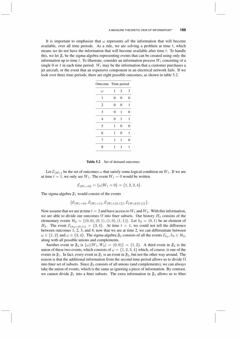
A MEASURE-THEORETIC VIEW OF INFORMATION** 189
It is important to emphasize that ω represents all the information that will becomeavailable, over all time periods. As a rule, we are solving a problem at time t, whichmeans we do not have the information that will become available after time t. To handlethis, we let Ft be the sigma-algebra representing events that can be created using only theinformation up to time t. To illustrate, consider an information process Wt consisting of asingle 0 or 1 in each time period. Wt may be the information that a customer purchases ajet aircraft, or the event that an expensive component in an electrical network fails. If welook over three time periods, there are eight possible outcomes, as shown in table 5.2.
Outcome Time period
ω 1 2 3
1 0 0 0
2 0 0 1
3 0 1 0
4 0 1 1
5 1 0 0
6 1 0 1
7 1 1 0
8 1 1 1
Table 5.2 Set of demand outcomes
Let EW1 be the set of outcomes ω that satisfy some logical condition onW1. If we areat time t = 1, we only see W1. The event W1 = 0 would be written
EW1=0 = ω|W1 = 0 = 1, 2, 3, 4.
The sigma-algebra F1 would consist of the events
EW1=0, EW1=1, EW1∈0,1, EW1 6∈0,1.
Now assume that we are at time t = 2 and have access toW1 andW2. With this information,we are able to divide our outcomes Ω into finer subsets. Our history H2 consists of theelementary events H2 = (0, 0), (0, 1), (1, 0), (1, 1). Let h2 = (0, 1) be an element ofH2. The event Eh2=(0,1) = 3, 4. At time t = 1, we could not tell the differencebetween outcomes 1, 2, 3, and 4; now that we are at time 2, we can differentiate betweenω ∈ 1, 2 and ω ∈ 3, 4. The sigma-algebra F2 consists of all the events Eh2
, h2 ∈ H2,along with all possible unions and complements.
Another event in F2 is ω|(W1,W2) = (0, 0) = 1, 2. A third event in F2 is theunion of these two events, which consists of ω = 1, 2, 3, 4which, of course, is one of theevents in F1. In fact, every event in F1 is an event in F2, but not the other way around. Thereason is that the additional information from the second time period allows us to divide Ωinto finer set of subsets. Since F2 consists of all unions (and complements), we can alwaystake the union of events, which is the same as ignoring a piece of information. By contrast,we cannot divide F1 into a finer subsets. The extra information in F2 allows us to filter
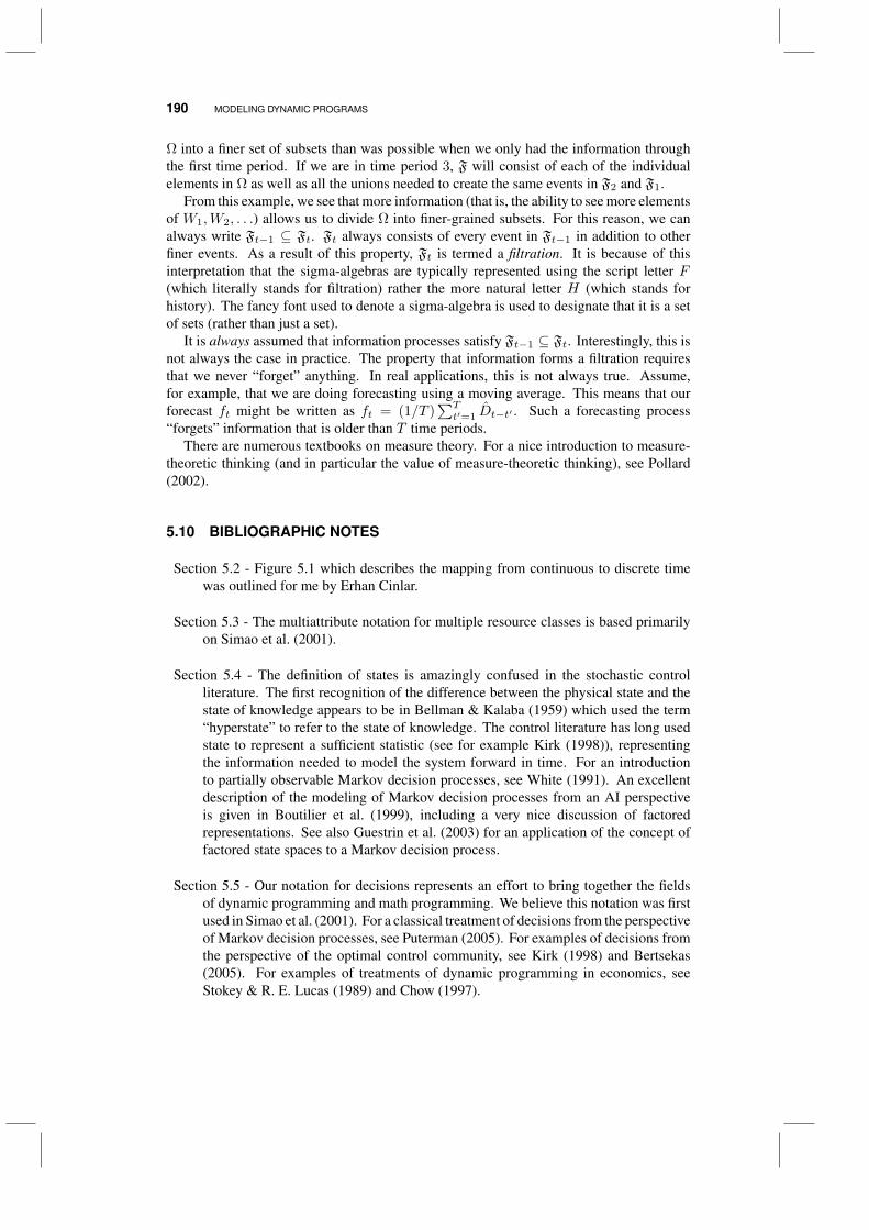
190 MODELING DYNAMIC PROGRAMS
Ω into a finer set of subsets than was possible when we only had the information throughthe first time period. If we are in time period 3, F will consist of each of the individualelements in Ω as well as all the unions needed to create the same events in F2 and F1.
From this example, we see that more information (that is, the ability to see more elementsof W1,W2, . . .) allows us to divide Ω into finer-grained subsets. For this reason, we canalways write Ft−1 ⊆ Ft. Ft always consists of every event in Ft−1 in addition to otherfiner events. As a result of this property, Ft is termed a filtration. It is because of thisinterpretation that the sigma-algebras are typically represented using the script letter F(which literally stands for filtration) rather the more natural letter H (which stands forhistory). The fancy font used to denote a sigma-algebra is used to designate that it is a setof sets (rather than just a set).
It is always assumed that information processes satisfy Ft−1 ⊆ Ft. Interestingly, this isnot always the case in practice. The property that information forms a filtration requiresthat we never “forget” anything. In real applications, this is not always true. Assume,for example, that we are doing forecasting using a moving average. This means that ourforecast ft might be written as ft = (1/T )
∑Tt′=1 Dt−t′ . Such a forecasting process
“forgets” information that is older than T time periods.There are numerous textbooks on measure theory. For a nice introduction to measure-
theoretic thinking (and in particular the value of measure-theoretic thinking), see Pollard(2002).
5.10 BIBLIOGRAPHIC NOTES
Section 5.2 - Figure 5.1 which describes the mapping from continuous to discrete timewas outlined for me by Erhan Cinlar.
Section 5.3 - The multiattribute notation for multiple resource classes is based primarilyon Simao et al. (2001).
Section 5.4 - The definition of states is amazingly confused in the stochastic controlliterature. The first recognition of the difference between the physical state and thestate of knowledge appears to be in Bellman & Kalaba (1959) which used the term“hyperstate” to refer to the state of knowledge. The control literature has long usedstate to represent a sufficient statistic (see for example Kirk (1998)), representingthe information needed to model the system forward in time. For an introductionto partially observable Markov decision processes, see White (1991). An excellentdescription of the modeling of Markov decision processes from an AI perspectiveis given in Boutilier et al. (1999), including a very nice discussion of factoredrepresentations. See also Guestrin et al. (2003) for an application of the concept offactored state spaces to a Markov decision process.
Section 5.5 - Our notation for decisions represents an effort to bring together the fieldsof dynamic programming and math programming. We believe this notation was firstused in Simao et al. (2001). For a classical treatment of decisions from the perspectiveof Markov decision processes, see Puterman (2005). For examples of decisions fromthe perspective of the optimal control community, see Kirk (1998) and Bertsekas(2005). For examples of treatments of dynamic programming in economics, seeStokey & R. E. Lucas (1989) and Chow (1997).

PROBLEMS 191
Section 5.6 - Our representation of information follows classical styles in the probabilityliterature (see, for example, Chung (1974)). Considerable attention has been givento the topic of supervisory control. An example includes Werbos (1992b).
PROBLEMS
5.1 A college student must plan what courses she takes over each of eight semesters. Tograduate, she needs 34 total courses, while taking no more than five and no less than threecourses in any semester. She also needs two language courses, one science course, eightdepartmental courses in her major and two math courses.
(a) Formulate the state variable for this problem in the most compact way possible.
(b) Give the transition function for our college student assuming that she successfullypasses any course she takes. You will need to introduce variables representing herdecisions.
(c) Give the transition function for our college student, but now allow for the randomoutcome that she may not pass every course.
5.2 Assume that we have N discrete resources to manage, where Ra is the number ofresources of type a ∈ A and N =
∑a∈ARa. Let R be the set of possible values of the
vector R. Show that
|R| =(
N + |A| − 1|A| − 1
),
where (XY
)=
X!
Y !(X − Y )!
is the number of combinations of X items taken Y at a time.
5.3 A broker is working in thinly traded stocks. He must make sure that he does not buyor sell in quantities that would move the price and he feels that if he works in quantitiesthat are no more than 10 percent of the average sales volume, he should be safe. He tracksthe average sales volume of a particular stock over time. Let vt be the sales volume onday t, and assume that he estimates the average demand ft using ft = (1− α)ft−1 + αvt.He then uses ft as his estimate of the sales volume for the next day. Assuming he startedtracking demands on day t = 1, what information would constitute his state variable?
5.4 How would your previous answer change if our broker used a 10-day moving averageto estimate his demand? That is, he would use ft = 0.10
∑10i=1 vt−i+1 as his estimate of
the demand.
5.5 The pharmaceutical industry spends millions managing a sales force to push theindustry’s latest and greatest drugs. Assume one of these salesmen must move between aset I of customers in his district. He decides which customer to visit next only after hecompletes a visit. For this exercise, assume that his decision does not depend on his priorhistory of visits (that is, he may return to a customer he has visited previously). Let Sn behis state immediately after completing his nth visit that day.

192 MODELING DYNAMIC PROGRAMS
(a) Assume that it takes exactly one time period to get from any customer to any othercustomer. Write out the definition of a state variable, and argue that his state is onlyhis current location.
(b) Now assume that τij is the (deterministic and integer) time required to move fromlocation i to location j. What is the state of our salesman at any time t? Be sureto consider both the possibility that he is at a location (having just finished with acustomer) or between locations.
(c) Finally assume that the travel time τij follows a discrete uniform distribution betweenaij and bij (where aij and bij are integers)?
5.6 Consider a simple asset acquisition problem where xt is the quantity purchased atthe end of time period t to be used during time interval t + 1. Let Dt be the demand forthe assets during time interval t. Let Rt be the pre-decision state variable (the amount onhand before you have ordered xt) and Rxt be the post-decision state variable.
(a) Write the transition function so that Rt+1 is a function of Rt, xt, and Dt+1.
(b) Write the transition function so that Rxt is a function of Rxt−1, Dt, and xt.
(c) Write Rxt as a function of Rt, and write Rt+1 as a function of Rxt .
5.7 As a buyer for an orange juice products company, you are responsible for buyingfutures for frozen concentrate. Let xtt′ be the number of futures you purchase in year t thatcan be exercised during year t′.
(a) What is your state variable in year t?
(b) Write out the transition function.
5.8 A classical inventory problem works as follows. Assume that our state variableRt isthe amount of product on hand at the end of time period t and that Dt is a random variablegiving the demand during time interval (t− 1, t) with distribution pd = P (Dt = d). Thedemand in time interval tmust be satisfied with the product on hand at the beginning of theperiod. We can then order a quantity xt at the end of period t that can be used to replenishthe inventory in period t+ 1. Give the transition function that relates Rt+1 to Rt.
5.9 Many problems involve the movement of resources over networks. The definition ofthe state of a single resource, however, can be complicated by different assumptions for theprobability distribution for the time required to traverse a link. For each example below,give the state of the resource:
(a) You have a deterministic, static network, and you want to find the shortest path froman origin node q to a destination node r. There is a known cost cij for traversingeach link (i, j).
(b) Next assume that the cost cij is a random variable with an unknown distribution.Each time you traverse a link (i, j), you observe the cost cij , which allows you toupdate your estimate cij of the mean of cij .
(c) Finally assume that when the traveler arrives at node i he sees cij for each link (i, j)out of node i.

PROBLEMS 193
(d) A taxicab is moving people in a set of cities C. After dropping a passenger off atcity i, the dispatcher may have to decide to reposition the cab from i to j, (i, j) ∈ C.The travel time from i to j is τij , which is a random variable with a discrete uniformdistribution (that is, the probability that τij = t is 1/T , for t = 1, 2, . . . , T ). Assumethat the travel time is known before the trip starts.
(e) Same as (d), but now the travel times are random with a geometric distribution (thatis, the probability that τij = t is (1− θ)θt−1, for t = 1, 2, 3, . . .).
5.10 In the figure below, a sailboat is making its way upwind from point A to point B.To do this, the sailboat must tack, whereby it sails generally at a 45 degree angle to thewind. The problem is that the angle of the wind tends to shift randomly over time. Theskipper decides to check the angle of the wind each minute and must decide whether theboat should be on port or starboard tack. Note that the proper decision must consider thecurrent location of the boat, which we may indicate by an (x, y) coordinate.
A
B
Path of boat:
Wind:
Port tack:
Starboard tack:
(a) Formulate the problem as a dynamic program. Carefully define the state variable,decision variable, exogenous information and the contribution function.
(b) Use δ to discretize any continuous variables (in practice, you might choose differentlevels of discretization for each variable, but we are going to keep it simple). Interms of δ, give the size of the state space, the number of exogenous outcomes (in asingle time period) and the action space. If you need an upper bound on a variable(e.g. wind speed), simply define an appropriate variable and express your answer interms of this variable. All your answers should be expressed algebraically.
(c) Using a maximum wind speed of 30 miles per hour and δ = .1, compute the size ofyour state, outcome and action spaces.
5.11 Implement your model from exercise 5.10 as a Markov decision process, and solveit using the techniques of 3 (section 3.2). Choose a value of δ that makes your programcomputationally reasonable (run times under 10 minutes). Let δ be the smallest value ofδ that produces a run time (for your computer) of under 10 minutes, and compare your
194 MODELING DYNAMIC PROGRAMS
solution (in terms of the total contribution) for δ = δN for N = 2, 4, 8, 16. Evaluate thequality of the solution by simulating 1000 iterations using the value functions obtained usingbackward dynamic programming. Plot your average contribution function as a function ofδ.
5.12 What is the difference between the history of a process, and the state of a process?
5.13 As the purchasing manager for a major citrus juice company, you have the respon-sibility of maintaining sufficient reserves of oranges for sale or conversion to orange juiceproducts. Let xti be the amount of oranges that you decide to purchase from supplier i inweek t to be used in week t + 1. Each week, you can purchase up to qti oranges (that is,xti ≤ qti) at a price pti from supplier i ∈ I, where the price/quantity pairs (pti, qti)i∈Ifluctuate from week to week. Let s0 be your total initial inventory of oranges, and let Dt
be the number of oranges that the company needs for production during week t (this is ourdemand). If we are unable to meet demand, the company must purchase additional orangeson the spot market at a spot price pspotti .
(a) What is the exogenous stochastic process for this system?
(b) What are the decisions you can make to influence the system?
(c) What would be the state variable for your problem?
(d) Write out the transition equations.
(e) What is the one-period contribution function?
(f) Propose a reasonable structure for a decision rule for this problem, and call it Xπ .Your decision rule should be in the form of a function that determines how much topurchase in period t.
(g) Carefully and precisely, write out the objective function for this problem in terms ofthe exogenous stochastic process. Clearly identify what you are optimizing over.
(h) For your decision rule, what do we mean by the space of policies?
5.14 Customers call in to a service center according to a (nonstationary) Poisson process.Let E be the set of events representing phone calls, where te, e ∈ E is the time that thecall is made. Each customer makes a request that will require time τe to complete and willpay a reward re to the service center. The calls are initially handled by a receptionist whodetermines τe and re. The service center does not have to handle all calls and obviouslyfavors calls with a high ratio of reward per time unit required (re/τe). For this reason, thecompany adopts a policy that the call will be refused if (re/τe) < γ. If the call is accepted,it is placed in a queue to wait for one of the available service representatives. Assume thatthe probability law driving the process is known, where we would like to find the rightvalue of γ.
(a) This process is driven by an underlying exogenous stochastic process with elementω ∈ Ω. What is an instance of ω?
(b) What are the decision epochs?
(c) What is the state variable for this system? What is the transition function?

PROBLEMS 195
(d) What is the action space for this system?
(e) Give the one-period reward function.
(f) Give a full statement of the objective function that defines the Markov decisionprocess. Clearly define the probability space over which the expectation is defined,and what you are optimizing over.
5.15 A major oil company is looking to build up its storage tank reserves, anticipating asurge in prices. It can acquire 20 million barrels of oil, and it would like to purchase thisquantity over the next 10 weeks (starting in week 1). At the beginning of the week, thecompany contacts its usual sources, and each source j ∈ J is willing to provide qtj millionbarrels at a price ptj . The price/quantity pairs (ptj , qtj) fluctuate from week to week. Thecompany would like to purchase (in discrete units of millions of barrels) xtj million barrels(where xtj is discrete) from source j in week t ∈ 1, 2, . . . , 10. Your goal is to acquire20 million barrels while spending the least amount possible.
(a) What is the exogenous stochastic process for this system?
(b) What would be the state variable for your problem? Give an equation(s) for thesystem dynamics.
(c) Propose a structure for a decision rule for this problem and call it Xπ .
(d) For your decision rule, what do we mean by the space of policies? Give examples oftwo different decision rules.
(e) Write out the objective function for this problem using an expectation over theexogenous stochastic process.
(f) You are given a budget of $300 million to purchase the oil, but you absolutely mustend up with 20 million barrels at the end of the 10 weeks. If you exceed the initialbudget of $300 million, you may get additional funds, but each additional $1 millionwill cost you $1.5 million. How does this affect your formulation of the problem?
5.16 You own a mutual fund where at the end of each week t you must decide whetherto sell the asset or hold it for an additional week. Let rt be the one-week return (e.g.rt = 1.05 means the asset gained five percent in the previous week), and let pt be the priceof the asset if you were to sell it in week t (so pt+1 = ptrt+1). We assume that the returnsrt are independent and identically distributed. You are investing this asset for eventual usein your college education, which will occur in 100 periods. If you sell the asset at the endof time period t, then it will earn a money market rate q for each time period until timeperiod 100, at which point you need the cash to pay for college.
(a) What is the state space for our problem?
(b) What is the action space?
(c) What is the exogenous stochastic process that drives this system? Give a five timeperiod example. What is the history of this process at time t?
(d) You adopt a policy that you will sell if the asset falls below a price p (which weare requiring to be independent of time). Given this policy, write out the objectivefunction for the problem. Clearly identify exactly what you are optimizing over.