Dynamic Modelling of Proton Exchange Membrane Fuel Cells ...

DYNAMIC MODELLING OF PROTON EXCHANGE
MEMBRANE FUEL CELL SYSTEM FOR ELECTRIC
BICYCLE
AZADEH KHEIRANDISH
FACULTY OF ENGINEERING
UNIVERSITY OF MALAYA
KUALA LUMPUR
2016

DYNAMIC MODELLING OF PROTON EXCHANGE
MEMBRANE FUEL CELL SYSTEM FOR ELECTRIC
BICYCLE
AZADEH KHEIRANDISH
THESIS SUBMITTED IN FULFILMENT OF
THE REQUIREMENTS FOR THE DEGREE OF
DOCTOR OF PHILOSOPHY
FACULTY OF ENGINEERING
UNIVERSITY OF MALAYA
KUALA LUMPUR
2016

UNIVERSITY OF MALAYA
ORIGINAL LITERARY WORK DECLARATION
Name of Candidate: Azadeh Kheirandish
Registration/Matric No: KHA110083
Name of Degree: DOCTOR OF PHILOSOPHY
Title of Project Paper/Research Report/Dissertation/Thesis (“this Work”):
“DYNAMIC MODELLING OF PROTON EXCHANGE MEMBRANE FUEL
CELL SYSTEM FOR ELECTRIC BICYCLE”
Field of Study: AUTOMATION, CONTROL & ROBOTICS
I do solemnly and sincerely declare that:
(1) I am the sole author/writer of this Work;
(2) This Work is original;
(3) Any use of any work in which copyright exists was done by way of fair
dealing and for permitted purposes and any excerpt or extract from, or
reference to or reproduction of any copyright work has been disclosed
expressly and sufficiently and the title of the Work and its authorship have been
acknowledged in this Work;
(4) I do not have any actual knowledge nor do I ought reasonably to know
that the making of this work constitutes an infringement of any copyright work;
(5) I hereby assign all and every rights in the copyright to this Work to the
University of Malaya (“UM”), who henceforth shall be owner of the copyright
in this Work and that any reproduction or use in any form or by any means
whatsoever is prohibited without the written consent of UM having been first
had and obtained;
(6) I am fully aware that if in the course of making this Work I have
infringed any copyright whether intentionally or otherwise, I may be subject to
legal action or any other action as may be determined by UM.
Candidate’s Signature Date:
Subscribed and solemnly declared before,
Witness’s Signature Date:
Name:
Designation

iii
ABSTRACT
Fuel cell systems with high-energy efficiency provides clean energy with lower
noise and emissions that have attracted significant attention of energy. Proton exchange
membrane (PEM) fuel cell has high power density; long stack life and low-temperature
operation condition, which makes it a prime candidate for the vehicles. Performance
optimization of PEM fuel cell has been a topic of research in the last decade. The
efficiency of fuel cells is not specific; it is a subordinate to the power density where the
system operates. The fuel cell performance is least efficient when functioning under
maximum output power conditions.
Modelling the PEM fuel cell is the fundamental step in designing efficient
systems for achieving higher performance. In spite of affecting factors in PEM fuel cell
functionality, providing a reliable model for PEM fuel cell is the key of performance
optimization challenge. There have been two approaches for modelling and prediction of
commercial PEM fuel cell namely, theoretical and empirical models. Since theoretical
modeling is not achievable in experimental conditions, the empirical modeling has
attracted significant attention in researches. Various types of algorithms have been
utilized for modelling these systems to achieve a high accuracy for predicting the
efficiency and controlling the system.
Recent models provide high accuracies using complex systems and complicated
calculations using advanced optimization algorithms. However, designing an accurate
dynamic model for prediction and controlling the system in a real time condition is a
challenge in this field. By utilizing the state of the art soft computing algorithms in
modeling the technical systems to reduce the complexity of the models artificial neural
networks have had a great impact in this field. This study has multifold objectives and

iv
aim to design models for a 250W proton exchange membrane fuel cell system that is used
as the power plant in electric bicycle. Classical linear regression and artificial neural
networks as the most popular and accurate algorithms have been optimized and used for
modeling this system. In addition, for the first time fuzzy cognitive map has been utilized
in modeling PEM fuel cell system and targeted to provide a dynamic cognitive map from
the affective factors of the system. Controlling and modification of the system
performance in various conditions is more practical by correlations among the
performance factors of the PEM fuel cell resulted from fuzzy cognitive map. On the other
hand, the information of fuzzy cognitive map modeling is applicable for modification of
neural networks structure for providing more accurate results based on the extracted
knowledge from the cognitive map and visualization of the system’s performance.

v
ABSTRAK
Sistem sel bahan api dengan kecekapan tenaga tinggi menyediakan tenaga
bersih dengan kadar bunyi dan pelepasan yang lebih rendah telah menarik perhatian besar
tenaga. Sel bahan api membran pertukaran proton (PEM) fuel cell telah menjadi pilihan
utama untuk kenderaan kerana mempunyai ketumpatan kuasa yang tinggi ; kadar hidup
timbunan yang lama dan keadaan operasi di suhu rendah. Pengoptimuman prestasi PEM
fuel cell telah menjadi topik penyelidikan untuk beberapa dekad yang lalu. Kecekapan sel
bahan api tidak khusus ; ia adalah lebih rendah daripada ketumpatan kuasa di mana sistem
beroperasi. Prestasi sel bahan api kurang berkesan apabila ianya berfungsi di dalam
keadaan kuasa keluaran yang maksimum.
Pemodelan PEMFC adalah langkah asas dalam mereka bentuk sistem yang
cekap untuk mencapai prestasi yang lebih tinggi. Selain faktor-faktor yang
mempengaruhi prestasi PEMFC , menyediakan model yang boleh dipercayai adalah
kunci kepada cabaran untuk mengoptimumkan prestasi PEMFC. Terdapat dua
pendekatan untuk pemodelan dan ramalan komersial sel bahan api PEM iaitu model teori
dan model empirikal. Oleh kerana pemodelan teori tidak boleh dicapai daripada kajian ,
pemodelan empirikal telah menarik perhatian yang besar dalam penyelidikan. Pelbagai
jenis algoritma telah digunakan dalam pemodelan sistem ini untuk mencapai ketepatan
yang tinggi dalam meramal kecekapan dan mengawal sistem.
Model terbaru menyediakan ketepatan tinggi dengan menggunakan sistem
yang kompleks dan pengiraan yang rumit menggunakan algoritma pengoptimuman
paling maju. Walau bagaimanapun, mereka bentuk model dinamik yang tepat untuk
meramal dan mengawal sistem ini dalam keadaan masa sebenar adalah mencabar untuk
bidang ini. Dengan menggunakan keadaan seni algoritma pengkomputeran lembut dalam
pemodelan sistem teknikal untuk mengurangkan kerumitan model rangkaian neural tiruan

vi
mempunyai impak yang besar dalam bidang ini. Kajian ini mempunyai objektif berganda
dan bertujuan untuk mereka bentuk model untuk sebuah sistem sel bahan api membran
pertukaran proton berkuasa 250W yang digunakan sebagai loji kuasa dalam basikal
elektrik. Sebagai algoritma yang paling popular dan tepat, regresi linear klasik dan
rangkaian neural tiruan telah dioptimumkan dan digunakan untuk model sistem ini. Di
samping itu, buat kali pertama peta kognitif kabur telah digunakan dalam pemodelan
sistem sel bahan api PEM dan bertujuan untuk menyediakan peta kognitif dinamik dari
faktor keberkesanan sistem. Pengawalan dan pengubahsuaian prestasi sistem dalam
pelbagai keadaan adalah lebih praktikal dengan korelasi antara faktor prestasi sel bahan
api PEM hasil daripada peta kognitif kabur. Selain itu, maklumat daripada pemodelan
peta kognitif kabur boleh digunakan untuk pengubahsuaian struktur rangkaian neural
untuk memberikan hasil yang lebih tepat berdasarkan pengetahuan yang diekstrak dari
peta kognitif dan visualisasi prestasi sistem.

vii
ACKNOWLEDGMENT
I would like to express my special appreciation and thanks to my advisor Dr.
Mahidzal Dahari for the continuous support of my Ph.D study and related research, for
his patience, motivation, and his guidance and help during the time of my research. I
could not have imagined having a better advisor and mentor for my PhD study.
I would like to extend my thanks to my dear friend, Dr. Farid Motlagh for his
selfless support and professional research attitude that influenced me throughout my
whole graduate study. Besides, I would also like to thank my best friend, Assoc. Prof
Niusha Shafiabady for her kind support, guidance and her contributions to this research
are greatly appreciated. I would like to take this opportunity to express my appreciation
for my lovely friends: Sepideh Yazdani and Ali Askari and my beloved Jaana, for
standing beside me throughout this entire journey and providing their help and support in
many different ways.
A special thanks to my family for supporting me spiritually throughout writing
this thesis and my life in general. Words cannot express how grateful I am to my mother,
Azar Danesh, father, Reza Kheirandish, brother Mahyar and sister Mahsa for all of the
sacrifices that you’ve made on my behalf. Your prayer for me was the reason that has
sustained me this far. I would also like to thank all of my friends who supported me in
writing, and invited me to strive towards my goal.
Azadeh Kheirandish

viii
TABLE OF CONTENTS
ABSTRACT .................................................................................................................... iii
ABSTRAK ........................................................................................................................ v
ACKNOWLEDGMENT ................................................................................................. vii
TABLE OF CONTENTS .............................................................................................. viii
LIST OF FIGURE ......................................................................................................... xiii
LIST OF TABLES ........................................................................................................ xvii
LIST OF SYMBOLS AND ABBREVIATIONS ....................................................... xviii
LIST OF APPENDICES ............................................................................................. xxvii
Chapter 1 : INTRODUCTION .......................................................................................... 1
1.1 Background of study ................................................................................................ 1
1.2 Problem statement ................................................................................................... 6
1.3 Objectives ................................................................................................................ 7
1.4 Methodology ............................................................................................................ 8
1.5 Scope of the study ................................................................................................... 9
1.6 Outline of study ..................................................................................................... 10
Chapter 2 : LITERATURE REVIEW ............................................................................. 12
2.1 Introduction ......................................................................................................... 12
2.2 Background of the Study ..................................................................................... 13
Fuel Cell .................................................................................................... 13
2.2.1.1 Alkaline Fuel Cell (AFC)................................................................... 14
2.2.1.2 Direct Methanol Fuel Cell (DMFC) .................................................. 15

ix
2.2.1.3 Solid Oxide Fuel Cell (SOFC) ........................................................... 16
Molten Carbonate Fuel Cells (MCFC) .............................................. 17
Phosphoric Acid Fuel Cell (PAFC) ................................................... 18
Proton Exchange Membrane Fuel Cells (PEMFC) ............................ 19
2.2.2 Fuel Cell Applications ............................................................................... 24
2.2.2.1 Portable Power ................................................................................... 24
2.2.2.2 Stationary ........................................................................................... 25
2.2.2.3 Residential.......................................................................................... 26
2.2.2.4 Transportation .................................................................................... 27
2.3 Fuel cell efficiency .............................................................................................. 28
2.4 Fuel Cell Modeling.............................................................................................. 29
2.4.1 Theoretical Models .................................................................................... 29
2.4.2 Empirical Models ...................................................................................... 30
2.4.2.1 Linear Regression .............................................................................. 31
2.4.2.2 Artificial Neural Network Modelling ................................................ 32
2.4.2.2.1 Levenberg-Marquardt back propagation (LMBP) ......................... 32
2.4.2.3 Fuzzy Cognitive Map ......................................................................... 41
2.4.2.3.1 Learning Algorithms ..................................................................... 47
2.5 Summary ............................................................................................................. 51
Chapter 3 : METHODOLOGY ....................................................................................... 52
3.1 Introduction ......................................................................................................... 52
3.2 PEM fuel cell system........................................................................................... 54

x
3.2.1 Overall System Design (Electric Bicycle) ................................................ 54
3.2.2 PEM fuel cell powered bicycle ................................................................. 55
3.3 Data collection and analysis ................................................................................ 57
3.3.1 Data collection........................................................................................... 58
3.3.2 Variables selection procedure ................................................................... 58
3.4 Efficiency of fuel cell .......................................................................................... 59
3.5 Data-set............................................................................................................ 61
3.5.1 Data normalization .................................................................................... 62
3.5.2 Principle component analysis (PCA) ........................................................ 62
3.6 Regression models............................................................................................... 64
3.6.1 Linear Regression ...................................................................................... 65
3.6.1.1 Gradient Descent ................................................................................ 67
3.6.1.2 Learning curve ................................................................................... 68
3.6.2 Artificial Neural Network (ANN) ............................................................. 69
3.6.2.1 The Neural Network Basic Architecture............................................ 69
3.6.2.2 Network Architecture......................................................................... 71
3.6.3 Fuzzy Cognitive Map: ............................................................................... 73
3.6.3.1 Learning algorithm............................................................................. 76
3.6.3.1.1 Hebbian learning algorithm ........................................................... 77
3.6.3.1.2 Nonlinear Hebbian learning (NHL) ............................................... 77
3.6.3.1.3 Data-driven nonlinear Hebbian learning (DD-NHL) .................... 78
3.6.3.2 Rule base fuzzy cognitive maps (RB-FCMs) .................................... 83
xi
3.6.3.3 Linguistic variables influence for FCM weights ............................... 84
Chapter 4 : RESULTS AND DISCUSSION .................................................................. 87
4.1 Introduction ......................................................................................................... 87
4.2 Data collection..................................................................................................... 88
4.3 System efficiency ................................................................................................ 91
4.4 System modelling ................................................................................................ 96
4.4.1 Linear regression model ............................................................................ 97
4.4.2 Artificial neural networks model............................................................. 105
4.5 Fuzzy Cognitive Map .................................................................................... 116
4.5.1 FCM Training Process ......................................................................... 119
4.5.2 RB-FCM .............................................................................................. 123
Chapter 5 : CONCLUSION AND FUTURE WORK ................................................... 132
5.1 Conclusion ......................................................................................................... 132
5.2 Contributions ..................................................................................................... 134
5.3 Future work ....................................................................................................... 134
References ..................................................................................................................... 136
Appendix A ............................................................................................................... 150
Electric Bicycle and Experimental Device.................................................................... 150
A.1 Electric Bicycle ............................................................................................... 150
A.2 System Description ...................................................................................... 151
Appendix B ................................................................................................................ 159
Flow charts ................................................................................................................ 159

xii
B.1 State machine flow chart ............................................................................... 159
B.2 Start procedure flow chart ............................................................................. 160
B.3 Stop procedure flow chart ................................................................................... 161
Appendix C ................................................................................................................ 162
Fuel cell supervisor H2 software and data collection ................................................ 162
C.1 Fuel cell supervisor H2 ....................................................................................... 163
C.1.1 State of the system ........................................................................................... 164
C.1.2 System survey area .......................................................................................... 165
C.1.3 Data Collection ................................................................................................ 166
LIST OF PUBLICATIONS .......................................................................................... 175

xiii
LIST OF FIGURE
Figure 1.1: Ideal voltage versus current curve for fuel cell ............................................. 2
Figure 2.1: Alkaline fuel cell principle .......................................................................... 14
Figure 2.2: Direct methanol fuel cell principle .............................................................. 15
Figure 2.3: Solid oxide fuel cell principle ...................................................................... 16
Figure 2.4: Molten carbonate fuel cell principle ............................................................ 17
Figure 2.5: Phosphoric acid fuel cell.............................................................................. 18
Figure 2.6: The structure of proton electrolyte membrane ............................................ 19
Figure 2.7: Schematic of reaction in PEMFC's single cell ............................................ 21
Figure 2.8: Laptop computer powered by fuel cell ........................................................ 24
Figure 2.9: Fuel cells used for building ....................................................................... 25
Figure 2.10: Fuel cell used in a residential building .................................................... 26
Figure 2.11: Fuel cell used in transportation .................................................................. 27
Figure 2.12: regression model building ......................................................................... 31
Figure 2.13: Steps of neural network modelling approach ............................................ 33
Figure 3.1: Methodology flow chart .............................................................................. 53
Figure 3.2: Fuel cell-powered electric bicycle .............................................................. 54
Figure3.3: Block diagram of the fuel cell-powered electric bicycle system .................. 55
Figure3.4: Fuel Cell and auxiliary components ............................................................. 56
Figure 3.5: The panel of monitoring software for fuel cell system ................................ 57
Figure 3.6: qH2: hydrogen flow, qO2: oxygen flow, I: current load T: temperature, H:
humidity .......................................................................................................................... 63
Figure 3.7: Flowchart depicts the training process of regression models. Training and
validation datasets were used for model training and optimization of model parameters.
Test data set was used for evaluation of final design ...................................................... 65

xiv
Figure3.8: Linear regression configuration .................................................................... 65
Figure 3.9: Gradient decent ............................................................................................ 68
Figure3.10: Artificial Neuron configuration .................................................................. 70
Figure 3.11: Multiplayer Feedforward Network, where I: current, H2: hydrogen flow rate,
O2: oxygen flow rate, RH: related humidity and T: temperature as an inputs and V: voltage
and EFF efficiency of system as an outputs .................................................................... 71
Figure 3.12: Example of FCM graph and corresponding connection matrix ................ 74
Figure 3.13: Flowchart of NHL ..................................................................................... 80
Figure 3.14: Flow chart of DD-NHL ............................................................................. 82
Figure 3.15: Rule based fuzzy cognitive map structure ................................................. 83
Figure 3.16: Membership function for influence of the linguistic variables.................. 85
Figure 3.17: Flowchart of linguistic variable influence for FCM .................................. 86
Figure 4.1: Plot of the voltage‒current and power-current curves of Fuel Cell stack at
temperature average of 37.6 °C ....................................................................................... 89
Figure 4.2: Plot of Stack temperature and air humidity ratio versus current density of
Fuel Cell .......................................................................................................................... 91
Figure 4.3: Plot of FC stack efficiency versus FC stack output power for relatively
average temperature 37.6 ℃ over experiment period ..................................................... 92
Figure 4.4: Flow diagram for PEM fuel cell powered electric bicycle. This diagram
illustrates the various energy flows in system ................................................................. 93
Figure 4.5: Plot of fuel cell stack power measured during efficiency experiment ........ 95
Figure 4.6: MSE for training the data a) voltage b) efficiency ...................................... 98
Figure 4.7: Training of linear regression model for output a) voltage value b) efficiency
value .............................................................................................................................. 100
Figure 4.8: Evaluation of system performance based on input features ...................... 101
Figure 4.9: MSE for training, cross validation and testing a) voltage b) efficiency .... 102

xv
Figure 4.10: Comparison of predicted result and experimental data, a) voltage simulation
b) efficiency simulation by LR...................................................................................... 103
Figure 4.11: Predict the a) polarization curve and b) efficiency versus power by linear
regression (LR) and compare with experimental data of PEM fuel cell. ...................... 104
Figure 4.12: Scheme of function fitting NN model ..................................................... 105
Figure 4.13: Best validation performance of neural network model for output a) voltage
and b) efficiency value .................................................................................................. 107
Figure 4.14: Histogram of error for a) voltage output b) efficiency output ................. 108
Figure 4.15: Rates of correlation of output variables a) voltage b) efficiency by linear
regression for training ................................................................................................... 109
Figure 4.16: Correlation rate for testing patterns of outputs variable .......................... 110
Figure 4.17: Correlation rate of output variable a) voltage .......................................... 111
Figure 4.18: Comparison of predicted result and experimental data, a) voltage simulation
b) efficiency simulation by NN ..................................................................................... 113
Figure 4.19: Prediction of the polarization curve by NN and comparison with
experimental data of PEM fuel cell ............................................................................... 114
Figure 4.20: Prediction of efficiency versus power curve by NN and comparison with
experimental data of PEM fuel cell ............................................................................... 115
Figure 4.21: FCM scheme of PEM fuel cell system, I: current, T: temperature, RH:
related humidity, H2: hydrogen flow rate, O2: oxygen flow rate, V: voltage and Eff:
efficiency ....................................................................................................................... 119
Figure 4.22: Final FCM design of system. ................................................................... 121
Figure 4.23: MSE for training the data in FCM ........................................................... 122
Figure 4.24: Membership function for a) hydrogen flow rate b) Temperature c) Related
Humidity d) Efficiency.................................................................................................. 124
Figure 4.25: Membership function for influence matrix in electric bicycle system .... 126

xvi
Figure 4.26: Sample of RB-FCM relationship ............................................................. 127
Figure 4.27: Example of fuzzy rule for an interconnection ......................................... 130

xvii
LIST OF TABLES
Table 2-1: Comparison of fuel cell types. (OT defines Operating Temperature in
Centigrade scale) ............................................................................................................. 22
Table 2-2: Summary of previous works on ANN .......................................................... 38
Table 2-3: Examples of problems solved by FCM ......................................................... 43
Table 2-4: Learning approaches and algorithms for FCM ............................................. 49
Table 4-1: Nominal Fuel cell specifications................................................................... 88
Table 4-2: Fuel cell powered electric bicycle parameter measurements from data
demonstrated in Figure 4.5 (efficiency indicted by eff) .................................................. 94
Table 4-3: Men Square Error (MSE) for train, cross validation and test in linear
regression LR ................................................................................................................ 102
Table 4-4: Prediction result for different network architectures .................................. 106
Table 4-5: Performance of the best PEM fuel cell neural network model ................... 108
Table 4-6: Best linear fit for output variable for training, testing and validation ........ 112
Table 4.7 : Comparison MSE in artificial neural network (ANN) and linear regression
(LR) model .................................................................................................................... 115
Table 4-8: FCM connection matrix between 7 concepts of PEM fuel cell system ...... 117
Table 4-9: FCM connection matrix between 7 concepts of PEM fuel cell system in real
time modelling............................................................................................................... 118
Table 4-10: FCM connection matrix between 7 concepts of PEM fuel cell system in real
time modelling............................................................................................................... 120
Table 4-11: FCM connection matrix between four concepts of PEMFC..................... 123
Table 4-12: Type of value of FCM Concepts............................................................... 124

xviii
LIST OF SYMBOLS AND ABBREVIATIONS
Symbols
𝐻2 Hydrogen
𝑒 Electron
𝑂2 Oxygen
𝐻2𝑂 Water
OH− Hydroxide
CO2 Carbon
CH3OH Methanol
𝑐𝑜3= Carbonate
𝑉𝑜𝑝𝑒𝑟 Operation voltage
𝜂𝑓𝑐 Fuel cell efficiency
n Number of cells
ηfcsystem Efficiency of system
∆𝒑 Pressure drop
V volume (L) of an electrolyzer buffer tank
T Temperature (K)
n Number of random sample

xix
x Sample data with mean X ̅
S Standard deviation
z-score Standardization of data
𝑥 Explanatory variable
ℎ𝜃(𝑥) Predicted value (hypothesis)
𝜃0 Intercepts
𝜃 Estimated slope coefficient of the line
𝜀 Error term
y Real value
h Predicted value
MSE Mean of the squares
𝐽(𝜃) Cost function
m Number of iterations
𝛼 Learning rate value
𝜃 System weights
wkj Synaptic weights
xm Input
𝑘 Neuron
uk Linear combiner outputs

xx
𝑏𝑘 Bias
𝑣𝑘 Activation potential
𝜑(. ) Activation function
𝐹(𝑥) Sum of square error
x weights matrix and bias
𝐻(𝑥) Hessian matrix
(𝑥) Vector of network error
𝐽(𝑥) Jacobian matrix
𝐶𝑗(𝑡) Activation degree of concept 𝑗𝑡ℎ at moment t
𝑒𝑖𝑗 Relationship strength from concept 𝐶𝑖 to concept 𝐶𝑗
𝑐 Real positive number
𝑥 Value 𝐶𝑗(𝑡)
𝐶𝑖 Current activation of concept 𝑖𝑡ℎ
𝐶𝑖 Current activation of concept 𝑗𝑡ℎ
𝑒𝑖𝑗(𝑘) Value of the weights between concepts 𝑖𝑡ℎ 𝑎𝑛𝑑 𝑗𝑡ℎ
𝜂 Learning coefficient
𝐶(0) Value of concepts
𝐸(0) Connection matrix
𝑊𝐹𝐼𝑁𝐴𝐿 Final connection matrix

xxi
𝑇𝑗 Mean target value of the concept 𝐶𝑗
𝑒𝑚𝑎𝑥 Maximum difference
𝑑𝑖𝑗 Value of 𝑖𝑡ℎ concept at the 𝑗𝑡ℎ time point
𝐾 Number of available data points
𝑁 Number of concepts in modeled system
𝐴 Simulated data vector for every output parameter
T Real experimental value
N Sample number
𝐷𝐶𝑖𝑒𝑠𝑡𝑖𝑚𝑎𝑡𝑒𝑑 Estimated and of decision concepts (DC)
𝐷𝐶𝑖𝑟𝑒𝑎𝑙 Real value decision concepts (DC)
𝐾 Number of available iterations

xxii
ABBREVIATIONS
ICE Internal combustion engine
AFC Alkaline fuel cell
DMFC Direct methanol fuel cell
SOFC Solid oxide fuel cell
MCFC Molten carbonate fuel cell
PAFC Phosphoric acid fuel cell
PEMFC Proton exchange membrane fuel cell
ANFIS Adaptive neuro fuzzy inference system
ANN Artificial neural network
LR Linear regression
FCM Fuzzy cognitive map
DAQ Data acquisition
LHV Lower heating value
DD-NHL Data driven nonlinear Hebbian learning
RB-FCM Rule-based FCM
LMBP Levenberg-Marquardt back propagation
FCV Fuel cell vehicle

xxiii
GDL Gas diffusion layer
GA Genetic algorithm
BP Back propagation
RBF Radial basis function
NLP Non-linear programming
MPC Model predicted control
MBDO Metamodel-Based Design Optimization
EPSO Enhanced particle swarm optimization
IT Information technology
DCNs Dynamic Cognitive Networks
FGCMs Fuzzy Gray Cognitive Maps
IFCMs Intuitionistic Fuzzy Cognitive Maps
DRFCMs Dynamic Random Fuzzy Cognitive Maps
E-FCMs Evolutionary Fuzzy Cognitive Maps
FTCMs Fuzzy Time Cognitive Map
RCMs Rough Cognitive Maps
TAFCMs Timed Automata-based fuzzy cognitive maps
BDD-FCMs Belief-Degree Distributed Fuzzy Cognitive Maps
RBFCMs Rule Based Fuzzy Cognitive Maps

xxiv
FCN Fuzzy Cognitive Network
DHL Differential Hebbian Learning
BDA Balanced Differential Algorithm
NHL Nonlinear Hebbian Learning
AHL Active Hebbian Learning
ES Evolutionary Strategies
GA Genetic Algorithms
RCGA Real Coded Generic Algorithms
SI Swarm Intelligence
Mas Memetic Algorithms
SA Simulated Annealing
CSA Chaotic Simulated Annealing
TS Tabu Search
ACO Ant Colony Optimization
EGDA Extended Great Deluge Algorithm
BB-BC Bing Bang-Big Crunch
SOMA Self-Organizing Migration Algorithms
IA Immune Algorithms
NHL-DE Hebbian learning algorithm and Differential Evolution algorithm

xxv
NHL-EGDA Nonlinear Hebbian Learning algorithm and Extended Great
Deluge Algorithm
NHL-RCGA real-coded genetic algorithm and nonlinear Hebbian learning
algorithm
ECU Electronic Control Unit
HHV Higher heating value
R Ideal gas constant
RH Related humidity
I Current
qO2 Oxygen flow rate
T Temperature
qH2 Hydrogen flow rate
V fc Fuel cell voltage
Eff Efficiency
PCA Principle component analysis
GD Gradient Descent
m Number of measurements
n Number of trails
Wij Weights
DOC Desired Output Concepts

xxvi
mbf Membership functions
𝜇𝑛𝑣𝑠 Membership function negatively very strong
𝜇𝑛𝑠 Membership function negatively very strong
𝜇𝑛𝑚 Membership function negatively medium
𝜇𝑛𝑤 Membership function negatively weak
𝜇𝑧 Membership function zero
𝜇𝑝𝑤 Membership function positively weak
𝜇𝑝𝑚 Membership function positively medium
𝜇𝑝𝑠 Membership function positively strong
𝜇𝑝𝑣𝑠 Membership function positively very strong
DC Decision concepts

xxvii
LIST OF APPENDICES
Appendix A: Electric Bicycle and Experimental Device
Appendix B: Flow charts
Appendix C: Fuel cell supervisor H2 software and data collection

1
Chapter 1 : INTRODUCTION
1.1 Background of study
Fossil fuel depletion has created environmental problems such as pollution,
climate change and global warning. However, the largest fields of oil have been
discovered and production is clearly past its peak. Factors such as awareness of the health
problems related to high air pollution levels and dwindling oil fuel reserves have
increased interest in the replacement of internal combustion engine (ICE) vehicles.
However, considerable problems regarding health and environment are the result of the
use of too many vehicles worldwide, and for the sake of the health of the environment
and humanity, decreasing the use of fossil energy sources with the aim of zero emission
vehicles is helpful.
In vehicle industry, the major distinguished achievement is development of the
internal combustion engine vehicle (Brandon & Hommann, 1996; Chen, Hsaio, & Wu,
1992). To date, several automobile companies and research organizations regarding the
future generation of vehicles have focused on the production of hybrid vehicle technology
for enhancement of fuel economy, increased efficiency and controlled emission (Faiz,
Weaver, & Walsh, 1996; Kammen, 2002). Among the development of new energy
technologies fuel cells with sufficient efficiency and low emission are considered one of
the most promising vehicular power sources (Kordesch & Simader, 1996).

2
Figure 1.1 shows the theoretical voltage-current (V-I) curve of fuel cell for
considering how the fuel cell voltage varies with output current, and it also display cause
of voltage drop. Another important curve for developing the control strategy and
drivetrain topology for electric vehicle power by fuel cell is efficiency versus power.
Fuel cell powered electric vehicles have been considered a solution to the inherent
issue of long charge and short range time of electric vehicles compared to traditional
batteries. Fuel cells, discovered by British physicist William R Grove in 1839 (Blomen
& Mugerwa, 2013) are electrochemical energy conversion devices which generate
electricity by mixing hydrogen and oxygen in electrolyte. Fuel cells generate power with
low emission, high efficiency and quiet operation compared to conventional power
Figure 1.1: Ideal voltage versus current curve for fuel cell
Current density (MA/CM2)
0
0.5
1
Cel
l vo
ltage
Ideal or theoretical voltage
Total Loss
Operation voltage, V
Region of activation losses
Region of ohmic losses
Region of concentration losses

3
generator. Fuel cells are categorized into six variable types based on their electrolyte type
including:
1) Alkaline fuel cell (AFC) with a wide range of operation temperatures and are suitable
to use in spacecraft (McLean, Niet, Prince-Richard, & Djilali, 2002).
2) Direct methanol fuel cell (DMFC), a rare commonly used fuel cell which operates at
high temperature (Hamnett, 1997).
3) Solid oxide fuel cell (SOFC) with a high temperature threshold between 600 and
1000℃ (Hammou & Guindet, 1997).
4) Molten carbonate fuel cell (MCFC) to perform only at temperatures higher than 650℃
(Dicks, 2004).
5) Phosphoric acid fuel cell (PAFC) with operating temperature of 150-200℃ and is
utilized in both stationary power and mobile applications, such as large vehicles
(Bagotsky, 2012).
6) Proton exchange membrane fuel cell (PEMFC) with a lower operating temperature,
which renders the fuel cell viable for both portable and stationary applications
(Vishnyakov, 2006).
Power capacity of fuel cells are categorized according to their application
including portable power, stationary, residential, and transportation. Proton exchange
membrane fuel cell (PEMFC) is the most demanded type of fuel cell in popular
technology due to its simplicity, solid membrane, quiet operation and low temperature
operating range. In this project, PEM fuel cell has been used to run an electric bicycle.
Chemical reactions of PEM fuel cells are as follows:

4
Anode side: 2𝐻2 → 4𝐻+ + 4𝑒− (1-1)
Cathode side: 𝑂2 + 4𝐻+ + 4𝑒− → 2𝐻2𝑂 (1-2)
Net reaction: 2𝐻2 + 𝑂2 → 2𝐻2𝑂 (1-3)
Modelling plays a significant role in research projects by allowing investigation
of critical situations without presenting any real-life danger, which results in a better
evaluation of system. For accurate modeling and to define better efficiency of system,
PEM fuel cell modeling is required to draw the pattern for critical parameters. Several
models have been developed to improve the design and operation of fuel cells, especially
PEM fuel cell (Baschuk & Li, 2005; Ceraolo, Miulli, & Pozio, 2003; Contreras, Posso, &
Guervos, 2010; Gong & Cai, 2014; Haji, 2011; Meidanshahi & Karimi, 2012; Oezbek,
Wang, Marx, & Soeffker, 2013; Rowe & Li, 2001; Tiss, Chouikh, & Guizani, 2013),
based on theoretical and empirical modeling. Theoretical modeling involves solving
differential equations or integration or both to determine the PEM fuel cell performance
from various physical parameters. Empirical modeling predicts a model by using
experimental data without determining the process parameters in detail (Napoli, Ferraro,
Sergi, Brunaccini, & Antonucci, 2013).
Since PEM fuel cell is a complex nonlinear system with multi-variables,
optimizing model parameters for design improvement and performance enhancement
using analytical models is challenging. Mathematical nature of theoretical models make
them more complicated than empirical models (Ismail, Ingham, Hughes, Ma, &
Pourkashanian, 2014; Jang, Cheng, Liao, Huang, & Tsai, 2012). Therefore, advanced
algorithms are suggested to be developed in order to reduce the essential computational
effort (Gong & Cai, 2014; Samsun et al., 2014). Soft computing techniques and machine

5
learning algorithms are reliable mediums to employ in empirical modeling for a more
efficient prediction of affecting parameters on voltage–current (V–I) curve of fuel cell
(Boscaino, Miceli, & Capponi, 2013).
In recent years, active empirical modelling techniques based on machine learning
theory defined as adaptive neuro fuzzy inference system (ANFIS) (Rezazadeh, Mehrabi,
Pashaee, & Mirzaee, 2012; Silva et al., 2014; Vural, Ingham, & Pourkashanian, 2009),
support vector machine (SVM) (Q. Li, Chen, Liu, Guo, & Huang, 2014; Zhong, Zhu, &
Cao, 2006; Zhong, Zhu, Cao, & Shi, 2007), and artificial neural network (ANN) which is
a powerful tool for modelling the performance of PEM fuel cell (Jemeı, Hissel, Péra, &
Kauffmann, 2003; Lee, Park, Yang, Yoon, & Kim, 2004; Ogaji, Singh, Pilidis, &
Diacakis, 2006; S. Ou & L. E. Achenie, 2005) have been developed. The advantage of
these models over theoretical model is that they are much simpler, enabling quick
prediction and requiring less computational time.
Researches in this field aim to propose methods to predict the PEM fuel cell
performance and to compare it with experimental data to indicate the accuracy of the
model. Most of these studies applied algorithm to decrease the error in models.
Furthermore, some researchers have proposed a control technology for optimal control of
the system response (J. Hasikos, H. Sarimveis, P. Zervas, & N. Markatos, 2009; Jemeï,
Hissel, Péra, & Kauffmann, 2008; J.-M. Miao, Cheng, & Wu, 2011; Sachin V Puranik,
Ali Keyhani, & Farshad Khorrami, 2010; Wu, Shiah, & Yu, 2009). The focus of these
models is on the design of PEM fuel cell rather than its application.

6
1.2 Problem statement
Recent development in fuel cell efficiency and performance is based on single cell
or fuel cell while computing the whole system efficiency plays significant role to improve
the performance and efficiency of the system. Despite a number of limitations of PEM
fuel cell like high production cost of hydrogen, essential features such as zero emission,
high efficiency and low operating temperature, fast start-up, make PEM fuel cells ideal
for transportation. There is considerable difference between the actual and ideal
efficiency of systems that their internal components are not changeable; therefore,
controlling these system to operate in an optimized condition is challenging. In addition,
both empirical and theoretical models of PEM fuel cell have been aimed to improve the
design and operation of fuel cells, but this cannot be achieved without providing an
accurate and reliable model of the system. Although there have been numerous fuel cell
stack models in order to benefit from its design (Buchholz & Krebs, 2007; Hu, Cao, Zhu,
& Li, 2010; Kong & Khambadkone, 2009; Kong, Yeau, & Khambadkone, 2006; Rouss
et al., 2008; Zhang, Pan, & Quan, 2008), there has been few models for the whole PEM
fuel cell system (Ahmed M Azmy & István Erlich, 2005; Jemeı et al., 2003; Jemeï et al.,
2008).
Simulation model of whole fuel cell system in electric vehicle is essential to adjust
the optimization ability of complete vehicle with auxiliary component. Therefore, the
problem statement can be stated as developing a dynamic model for fuel cell system in
electric bicycle with the ability to predict each variable of PEM fuel cell and the efficiency
of whole system, providing a cognitive map from the PEM fuel cell with a linguistic
relationship between variables to be used for control and real-time processing
applications.

7
1.3 Objectives
Cognitive map can be used to evaluate the performance of PEMFC system and
enable it to be used for controlling all variables in order to increase the efficiency .The
main goal of this study is dynamic modelling of the PEM fuel cell performance in electric
bicycle. The objectives of this study are as follows:
1- To define an accurate relation between efficiency and power density of system
during different operation conditions based on experimental data.
2- To design a linear regression model for predicting output voltage and system
efficiency based on (temperature, related humidity, current, hydrogen/oxygen
flow rate).
3- To improve and optimize the PEM fuel cell empirical model using artificial neural
networks.
4- To develop a fuzzy cognitive map (FCM) of PEM fuel cell variables and to
provide the causality of these variables on each other for real-time control
applications.

8
1.4 Methodology
The data has been collected from data acquisition (DAQ). Values of (temperature,
related humidity, current, hydrogen/oxygen flow rate and voltage) were recorded from
the PEM fuel cell system. With reference to the problem statement and objectives of this
study, methodology is illustrated in separate phases. First phase of the study aims to
define an accurate relation between efficiency and power density of system during
different operation conditions based on experimental data. Fuel cell efficiency was
calculated by using fuel cell's stack operating voltage (𝑉𝑜𝑝𝑒𝑟) versus hydrogen’s lower
heating value (LHV) equation. Since in the PEM fuel cell single cells are connected in
series, the efficiency of single cell and fuel cell stack are equal. The whole system’s
efficiency has been computed using generated electric bicycle energy versus energy of
consumed H2. A detailed description of equations can be found in chapter 3.
In the second phase of the study, various models of PEM fuel cell were presented
for better understanding of fuel cell system behavior and operation process. Both linear
and non-linear models were used for modelling the PEM fuel cell electric bicycle: 1)
linear regression model and 2) artificial neural network model and comparison of these
two models for better performance estimation of PEM fuel cell system. These models
were designed based on available variables including load current, temperature, related
humidity, and hydrogen/oxygen flow rate as inputs with load voltage and system
efficiency as output variables. Each of these models have been optimized in order to
minimize the cost function of models and represent optimal value of decision variables to
provide an accurate prediction of outputs.
Since using classical control theories to design a controller for system could
compromise the efficiency of the system, in the final phase of this study a dynamic model
was used to predict the system status based on the causality relations among PEM fuel

9
cell variables. Fuzzy cognitive map (FCM) was used for the first time as a convenient and
powerful tool for dynamic system modelling based on experimental data. FCM is a
combination of fuzzy logic and neural network through strategy of relation between all
factors. Data driven nonlinear Hebbian learning method (DD-NHL) was used as a state
of the art algorithm to design the cognitive map of PEMFC. FCM has been trained by the
collected data to generate accurate causality relations between variables. The causality
relations in this model were converted into fuzzy concepts in order to provide a rule-based
FCM (RB-FCM). The main advantage of RBFCM is the flexibility of the model for
providing an accurate dynamic model of the system for real-time control applications.
1.5 Scope of the study
In this study, a 25-Kg electric assisted bicycle special VRLA-battery 6-DZM-10
12V 10Ah is used to determine the overall efficiency of the system by using experimental
data. The data collection is performed on a stationary bicycle while the tire could spin
freely on traditional Kickstand. For this experiment, we attempted to keep the bicycle at
the cruise condition (constant speed) with a fuel cell power average of 35.29 W, and fuel
cell stack efficiency average of 48.45%. Parameters in the condition of this test are
obtained in ambient temperature range 0℃ up to 35 ℃ and ambient relative humidity
range of 30-80%.
The linear model was designed based on gradient descent algorithm and ANN was trained
using Levenberg-Marquardt back propagation (LMBP) algorithm. Validation data was
used to plot learning curve and error analysis for optimizing the models variables and
structure. The RBFCM was used only for dynamic modeling of the system variables.
However, due to the limited accessibility to inner auxiliaries and parameters of bicycle

10
and PEMFC, real-time control of the system input parameters was not feasible. However,
the final design of RBFCM was accurate for dynamic training and prediction of system
status to be used for controllers.
1.6 Outline of study
This thesis has been organized into five chapters.
Chapter 1 (present chapter) outlines brief introduction of the research area starting
with the fuel cell general overview, problem statement, objective, methodology, and
scope of the study. This chapter presents a general viewpoint to enable the reader to
understand what has been done in this project.
Chapter 2 provides a background about type of fuel cells and their application in
detail. This is followed by a discussion of the types of PEM fuel cell models and a brief
review of linear regression model and artificial neural network models as effective
methods to give a general idea of these empirical model approaches. The fuzzy cognitive
map and its application have been also introduced in this section.
Chapter 3 describes the methodology employed in the current study including
details of how data has been collected from bicycle and how the overall efficiency of
system was calculated. The proposed procedure to model PEM fuel cell system is
provided step by step and investigated to find optimal parameters to obtain more accurate
and faster modelling. The fuzzy cognitive map was trained by using state of art Non-
linear Hebbian learning algorithm which has been elaborated in detail in chapter 3.

11
Chapter 4 presented the result and discussion of implementation of calculated
overall efficiency, linear regression and neural network prediction and fuzzy cognitive
map model.
Chapter 5 provides the conclusion of this thesis and recommendations for future
work.

12
Chapter 2 : LITERATURE REVIEW
2.1 Introduction
Over the past three decades, the major environmental issue in many countries
around the world has been the global warming, lead to a dramatic increase in electrical
energy demand. Many researchers have presented an alternative energy converter at an
affordable price. These converters are generally eco-friendly (Purkrushpan & Peng, 2004)
During the past decade, research and development of electric vehicles have
attracted significant attention due to various concerns such as reducing emission and air
pollution from the combustion of fossil fuels. This kind of promising technology has
minimum emission, significant improvement in fuel economy and higher efficiency than
today’s internal combustion engines (Kammen, 2002).
Currently, many researchers are working to produce clean electrical energy for
future generation vehicles. One of the major challenges has been the inherent limitation
of short range and long charge time historically related to electric power vehicles. The
ideal solution compared to traditional battery power electric vehicles is fuel cell powered
hybrid vehicles. The main focus of hybrid vehicles is electric cars and buses in developing
countries because of air pollution, and smaller vehicles are widely used for transportation
and utility purposes (Dockery et al., 1993). Z Qi (2009) (Garche et al., 2013)
demonstrated various vehicular applications, such as bicycles, wheelchairs, forklifts, and
scooters, that utilize PEM fuel cells instead of batteries.
Addressing all these issues surrounding the internal combustion engine vehicles
and replacing these with low-emission, renewable fuel and high energy efficiency, the

13
good choice currently is hydrogen fuel cell vehicle (FCVs) which provides the chance for
the consumer to be a both user and producer of energy (Rifkin, 2003). The background
of fuel cell vehicles and the remaining issues for getting these vehicles on the road are
discussed in section 2.3.
2.2 Background of the Study
Fuel Cell
A fuel cell is a device that releases a considerable amount of power in the form of
electrical currents as hydrogen and oxygen atoms undergo an electrochemical reaction,
the by-product of which is water molecules (F. Barbir & Gomez, 1997). A fuel cell is
similar to battery in convert of chemical energy to electric energy; however, one distinct
difference between them is that fuel cells continue to operate as long as fuel and air are
supplied and there is no need to recharge. Sir William Grove invented the fuel cell in
1839 based on C.F Schoenbein’s idea as he observed the fuel cell effect; Grove saw the
capability of combining oxygen and hydrogen to make water (Bossel, Schönbein, &
Grove, 2000)
Currently, fuel cells are categorized into six different types based on their
electrolyte material, fuel diversity and operating temperature that make them suitable for
different applications. The following sections briefly presented the main types of fuel
cells and section 2.1.1.6 provides more details the of proton exchange membrane fuel cell
(PEMFC).

14
2.2.1.1 Alkaline Fuel Cell (AFC)
Alkaline fuel cells (AFC) demonstrated by Francis Bacon in 1930 are one of most
popular fuel cells developed to power NASA’s Apollo space program. They contain an
alkaline solution derived from an alkaline electrolyte. They can operate over a wide range
of temperatures that depend on the fuel cell application, which constitutes the main
advantage of these fuel cells over the other types. However, the significant technical
disadvantage of this type of fuel cell is the carbon dioxide poisoning of the electrolyte.
They react with hydrogen at the anode, releasing four electrons and producing water:
At anode: 2H2 + 4OH− → 4H2O + 4e− (2-1)
Electrons react with oxygen and water at the cathode and produce new OH:
At cathode: O2 + 4e− + 2H2O → 4OH− (2-2)
For continuous reaction, the mobile ion OH− should pass through the electrolyte,
and for electrons to go from anode to cathode, there must be an electrical circuit (Lin,
Kirk, & Thorpe, 2006). Figure 2.1 displays the principle of alkaline fuel cell.
Anode: 2H2+4OH- 4H2O+4e-
OH- Ions through electrolyte
Cathode: O2+4e-+2H2O 4OH-
Load
Figure 2.1: Alkaline fuel cell principle

15
2.2.1.2 Direct Methanol Fuel Cell (DMFC)
Direct methanol fuel cell was discovered by Dr. Surya Prakash and Dr. George A.
Olah in 1990, and is the only fuel cell that consumes methanol for fuel instead of
hydrogen. The utilization of these fuel cells is limited to applications in which the
efficiency is superseded by the power density in terms of importance. Hence, the
utilization of DMFCs is not as common as that of other fuel cells. Methanol is mixed with
water at the anode and the mobile ion is H+ passes through the electrolyte and six
electrons are released and transferred from anode to cathode:
At the anode: CH3OH + H2O → 6H+ + 6e− + CO2 (2-3)
Electrons react with oxygen and hydrogen at the cathode and produce water:
At the cathode: 3
2O2 + 6H+ + 6e− → 3H2O (2-4)
Overall reaction: CH3OH +3
2O2 → 2H2O + CO2 (2-5)
The issue about DMFC is that CO2 is produced as a byproduct and the reaction at
the anode is slow and provides less power(Frano Barbir, 2012). Figure 2.2 shows the
principle of direct methanol fuel cell.
Figure 2.2: Direct methanol fuel cell principle
Anode: CH3OH+H2O 6H++6e-+CO2
H+ Ions through electrolyte
Cathode: 3
2O2+6H+6e- 3H2O
Load
16
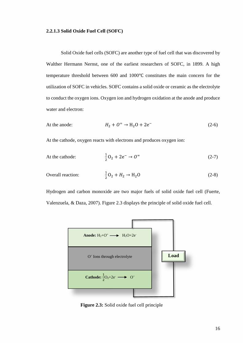
2.2.1.3 Solid Oxide Fuel Cell (SOFC)
Solid Oxide fuel cells (SOFC) are another type of fuel cell that was discovered by
Walther Hermann Nernst, one of the earliest researchers of SOFC, in 1899. A high
temperature threshold between 600 and 1000℃ constitutes the main concern for the
utilization of SOFC in vehicles. SOFC contains a solid oxide or ceramic as the electrolyte
to conduct the oxygen ions. Oxygen ion and hydrogen oxidation at the anode and produce
water and electron:
At the anode: 𝐻2 + 𝑂= → H2O + 2e− (2-6)
At the cathode, oxygen reacts with electrons and produces oxygen ion:
At the cathode: 1
2O2 + 2e− → 𝑂= (2-7)
Overall reaction: 1
2O2 + 𝐻2 → H2O (2-8)
Hydrogen and carbon monoxide are two major fuels of solid oxide fuel cell (Fuerte,
Valenzuela, & Daza, 2007). Figure 2.3 displays the principle of solid oxide fuel cell.
Anode: H2+O= H2O+2e-
O= Ions through electrolyte
Cathode: 1
2O2+2e- O=
Load
Figure 2.3: Solid oxide fuel cell principle

17
Molten Carbonate Fuel Cells (MCFC)
Molten carbonate fuel cell (MCFCs) was built by Erwin Baur in 1921 based on a
mixture of molten salts that act as an electrolyte. These fuel cells can perform only at
temperatures that are higher than 650℃. Carbonate and hydrogen react at the anode side
and produce water and 𝐶𝑂2and electron:
At the anode: 𝐻2 + 𝑐𝑜3= → H2O + CO2 + 2e− (2-9)
Oxygen and by carbon dioxide react with electrons at the anode and produce carbonate
anions.
At the cathode: 1
2O2 + CO2 + 2e− → 𝑐𝑜3
= (2-10)
The exothermic overall reaction is:
Overall reaction: 𝐻2 +1
2O2 + CO2 → H2O + CO2 (2-11)
To complete the circuit carbonate anions pass from the cathode to anode through
the molten electrolyte. During oxygen reduction, carbon dioxide is passed to the cathode
for use (Bischoff & Huppmann, 2002). Figure 2.4 shows the principle of molten carbonate
fuel cell.
Anode: H2+CO3= H2O+CO2+2e-
CO3= Ions through electrolyte
Cathode: 1
2O2+CO2+2e- CO3
=
Load
Figure 2.4: Molten carbonate fuel cell principle

18
Phosphoric Acid Fuel Cell (PAFC)
Phosphoric acid fuel cell (PAFCs) was developed by G. V. Elmore and H. A.
Tanner in 1961 and uses liquid phosphoric acid as an electrolyte. The operating
temperature of these devices is approximately (150-200)℃ . PAFCs are used in both
stationary power and mobile applications such as large vehicles. The pre-heating
requirements and its open-ended structure which requires the careful control of hydrogen
flow are some of its drawbacks. Pure hydrogen at the anode breaks into hydrogen ion and
produces four electrons.
At the anode: 2𝐻2 → 4H+ + 4e− (2-12)
Hydrogen ions and oxygen and electrons at the cathode produce water, and electrons pass
through the external circuit from anode to cathode.
At the cathode: O2 + 4H+ + 4e− → 2H2O (2-13)
Overall reaction: 2𝐻2 + O2 → 2H2O (2-14)
The output is very low at the anode due to pure hydrogen and using Carbon monoxide in
fuel increases it (Kasahara, Morioka, Yoshida, & Shingai, 2000). Figure 2.5 displays the
principle of phosphoric acid fuel cell.
Anode: 2H2 4H++4e-
CO3= Ions through electrolyte
Cathode: O2+ 4H+ +4e- 2H2O
Load
Figure 2.5: Phosphoric acid fuel cell

19
Proton Exchange Membrane Fuel Cells (PEMFC)
Proton exchange membrane fuel cell was invented by Willard Thomas Grubb and
Leonard Niedrach of General Electric in the early 1960s. Some issues that accrued in fuel
cells are removed; i.e. the requirement for expensive material, application in extreme
conditions and it is one of the most promising systems that can be used for stationary
application due to their size. In recent years, the high efficiency of PEMFCs has provided
impressive capabilities for the transportation sector. Low temperature, high efficiency,
silence and simplicity are distinguishing features that set PEMFCs apart from other fuel
cells and allow PEM fuel cell to be operated in any orientation and easy start-up
(Kheirandish, Kazemi, & Dahari, 2014).
Polymer membrane, catalyst layer, gas diffusion layer, and bipolar plate are the
main components of PEM fuel cells. Polymer membrane located on the center of the fuel
cell, separates the anode and cathode and hydrogen ions that pass through it. Hydrogen
oxidation and oxygen reduction react on catalyst layer at anode and cathode respectively.
Gas diffusion layer (GDL) is after catalyst layer at anode and cathode. These three layers
are called membrane electrode assembly. The MEA is plated between bipolar plate that
is commonly made of graphite (Larminie, 2003; Liu & Case, 2006). Figure 2.6 shows the
structure of polymer electrolyte membrane.
O2H2
2e-
Bipolar plate
ANODE
GDL Catalyst
layer Bipolar plate
Cathode
Catalyst
layer GDL
Mem
br
ane
H2
H2
H2
Air
Air
Air 2H+
1 2O
2+
2H
++
2e−
→H
2O
𝐻2
→2
H+
+2
e−
Figure 2.6: The structure of proton electrolyte membrane

20
Similar to other types of fuel cells, PEMs also consists of three significant parts:
a cathode and an anode that act as electrolytes formed by platinum-catalysis and the
membrane(Cook, 2002). In a PEM fuel cell reflex, the hydrogen oxidation and oxygen
reduction reactions occur simultaneously at the anode and cathode (Asl, Rowshanzamir,
& Eikani, 2010). Figure 2.7 shows the single cell of a fuel cell.
At the anode, the stream of hydrogen molecules are disarticulated into protons and
electrons as follows:
At the anode: 𝐻2 → 2H+ + 2e− (2-15)
Electrons are released from hydrogen and move along the external load circuit to
the cathode; therefore, the flow of electrons creates the electrical output current. The
electron arriving at the cathode from the external circuit concurrently reacts with oxygen
molecules that are joined with a platinum catalyst of electrode and two protons (which
have moved through the membrane) to create water molecules; this reduction is
represented as follows:
At the cathode: 1
2O2 + 2H+ + 2e− → H2O (2-16)
Overall reaction: 𝐻2 +1
2O2 → H2O (2-17)
The chemical reaction is now complete. Despite the reaction, a portion of the
energy is expended in the form of heat released from the respective redox reaction as a
byproduct.
The typical single cell voltage produces 0.5-0.7 V under load condition to have maximum
power. The single cells must be connected in series to create adequate electricity.

21
PEM fuel cells are used in many applications without geographical restrictions,
and their superior efficiency is being capitalized on in automobiles [for more detailed
information see: (Baschuk & Li, 2000; Marr & Li, 1999)]. Using a proton conductive
polymer membrane as an electrolyte leads to lower operating temperatures, which render
the fuel cell viable for both portable and stationary applications. Factors such as being
lightweight, a minuscule amount of corrosive fluid, a long stack lifetime, the generation
of zero emissions, and higher efficiencies, render this fuel cell to be perfect for automobile
applications (Yilanci, Dincer, & Ozturk, 2008)
A low temperature and high efficiency are two distinguishing features that set
PEMFCs apart from other fuel cells (Wee, 2007). The operating temperature range of
PEMFCs is 50-100℃, leads to a very quick commissioning ability. The total cost is also
rather low because cheaper materials are viable at low temperature settings as the
operation carries less risks. The efficiency of a PEM fuel cell is also much higher
compared to that of an internal combustion engine in vehicles while direct hydrogen acts
Fuel (Hydrogen)
2𝐻2
Oxygen
𝑂2
Water
2𝐻2𝑂
Proton exchange membrane (PEM)
Figure 2.7: Schematic of reaction in PEMFC's single cell

22
as its input. Furthermore, the small load on a PEM fuel cell translates into higher
efficiencies. For a normal driving time, a vehicle will require only a small amount of
nominal engine power, and a PEM fuel cell is especially poignant in this regard because
its efficiency is maximized when the loads are small. This efficiency peak stands in
contrast to that of an internal combustion engine (Salemme, Menna, & Simeone, 2009).
Evaluation between different types of fuel cells are shown in Table 2-1(Larminie, Dicks,
& McDonald, 2003).
Table 2-1: Comparison of fuel cell types. (OT defines Operating Temperature in
Centigrade scale)
Fuel cell
type Electrolyte OT Application Advantages Disadvantages
Alkaline
Fuel Cell
(AFC)
Potassium
hydroxide 90-100
Military
space
-Simple operation
- low weight &
volume
- low temperature
- not have
corrosion problems
-extremely intolerant
to CO2
- relatively short
lifetime
Direct
Methanol
Fuel Cell
(DMFC)
Solid
polymer
membrane
0-100
Consumer
goods
Laptop
Mobile phones
- Easy storage and
transport
-High energy
storage
- low power output
with respect to the
hydrogen cells
- Methanol is toxic
and flammable
Solid Oxide
Fuel Cell
(SOFC)
Ceramic
oxide
650-
1000
Electric utility
Auxiliary
power
Large
distributed
generation
-Fuel flexibility
- Very fast
chemical reactions
-high efficiency
-slow start up
- high temperature
enhances corrosion &
breakdown of cell
component
- Not a mature
technology

23
Table 2.1 continued:
Fuel cell
type Electrolyte OT Application Advantages Disadvantages
Molten
Carbonate
Fuel Cells
(MCFC)
Alkali
carbonates
600-
700
Electric utility
Large
distributed
generation
-High speed reaction
-High efficiency
-suitable for combine heat
and power
-Slow start up
-Complex
electrolyte
management
- Require
preheating
before starting
work
Phosphoric
Acid Fuel
Cell
(PAFC)
Phosphorous 150-
200
Distributed
generation
-Use air directly
from atmosphere
-high overall
efficiency with
CHP
-low current and
power
-large size
-requires expensive
platinum catalyst
Proton
Exchange
Membrane
Fuel Cells
(PEMFC)
Solid
polymer
membrane
50-
100
Small
distributed
generation
Backup power
Portable power
Transportation
-Low
temperature
-Quick start
-Solid electrolyte
reduces
corrosion&
electrolyte
management
problems
-compact and
robust
-simple
mechanical design
-High efficiency
-High sensitivity fuel
impurities
-very expensive
catalyst (platinum) and
a membrane (solid
polymer)
-Low temperature
-Waste heat
temperature not
Suitable for combined
heat & power

24
2.2.2 Fuel Cell Applications
The electrical power produced by different types of fuel cells, ranges from
milliwatts to megawatts. The application of fuel cells has been categorized based on their
power capacity can be summarized as follows.
2.2.2.1 Portable Power
Fuel cells are developed to power portable devices such as cellular phone without
recharging up to a month and power laptops longer than batteries. Fuel cells also can
power digital handheld devices such as video recorder, pagers, portable power tools and
low power remote devices such as smoke detectors, hotels locks and hearing aids. Proton
exchange membrane (PEM) and Direct Methanol Fuel Cell (DMFC) are two fuel cells
used as portable power banks. Figure 2.8 shows a laptop powered by fuel cell. (Dyer,
2002; Salameh, 2014).
Figure 2.8: Laptop computer powered by fuel cell
(source: http://www.hydrogengas.biz/hydrogenfuelcelllaptop.html)

25
2.2.2.2 Stationary
Fuel cell systems can provide the main power for building applications such as
schools, hotels, office buildings, and for back up the power for critical place such as
airports and hospitals. Four stationary types of fuel cells that can be employed to generate
power include solid oxide (SOFC), molten carbonate (MCFC), phosphoric acid (PAFC)
and proton exchange membrane (PEM) fuel cells. Figure 2.9 shows a building that uses
fuel cell to produce power(Salameh, 2014).
Figure 2.9: Fuel cells used for building
(source: http://www.fuelcells.org/uploads/bloom_constellation-place.jpg)

26
2.2.2.3 Residential
For small commercial and residential applications, small fuel cell could be
applied. Clear Edge manufactures PEM fuel cells to generate power and heat
simultaneously to warm swimming pools and provide hot water. Moreover, hot water or
heating for home can use the heat from the reaction. Proton exchange membrane (PEM)
fuel cell generally used in residential and small commercial building. Figure 2.10 shows
the fuel cell uses in residential buildings (Salameh, 2014).
Figure 2.10: Fuel cell used in a residential building
(source:http://www.cleantechinvestor.com/portal/interviews/1765-the-hydrogen-
home.html)

27
2.2.2.4 Transportation
Design of vehicle powered by fuel cells is one of the solutions to the increasing
cost of gasoline fuel and natural gas. Currently, fuel cells are developed for use in various
vehicles such as buses, cars, forklifts, golf carts, airplanes, motorcycle, scooters and
bicycles. In today’s society, electric bicycle has become more popular as it is cost
effective and more reliable. The fuel cells that are applied in this application are proton
exchange (PEM) fuel cells. Figure 2.11 shows the fuel cells applied in a car (Salameh,
2014).
Figure 2.11: Fuel cell used in transportation
(source: http://www.fuelcells.org/uploads/Picture-003.jpg)

28
2.3 Fuel cell efficiency
During the past decade, detailed theoretical efficiency calculation methods have
drawn increasing attention in many available publications for better performance of PEM
fuel cell. Low efficiency and high production cost are some of the most serious challenges
for previous fuel cell technologies. Therefore, many research groups have focused on this
area as a key challenge for the commercialization stage. Fuel cells are expected to
generate power for longer periods and at higher efficiencies compared to batteries.
Barbir and Gomez (1996) (Frano Barbir & Gomez, 1996) investigated the primary
rule of efficiency of PEM fuel cell and surmised that the economics and operating
efficiency of a fuel cell are interrelated. Kazim (Kazim, 2002, 2004, 2005) presented a
novel approach on the determination on minimal operating efficiency in PEM fuel cell
and its performance in different conditions. Ferng et al. (Ferng, Tzang, Pei, Sun, & Su,
2004) investigated the performance of single-cell PEM fuel cell analytically and
experimentally. Yongping Hou et al. (Hou, Zhuang, & Wan, 2007) proposed models that
detail the efficiency of fuel cells and investigated their theoretical and experimental
efficiency while evaluating several influencing parameters that are related to the
efficiency of a fuel cell. Meiyappan Siva Pandian (2010) (Pandian, Anwari, Husodo, &
Hiendro, 2010) stipulated that enhancing the power output of PEM would reduce the
efficiency, which would be detrimental to the economic aspect of the system. They carried
out performance and efficiency testing of PEM fuel cell in different operating temperature
and pressure.
In order to improve the efficiency and system performance of power density,
optimization of product and to design a PEM fuel cell system in various conditions is very
important and challenging.

29
2.4 Fuel Cell Modeling
A key issue for effective and efficient utilization of the PEM fuel cells and solar
cells is optimal modelling. Models have been developed to represent the behaviour of the
system at different operating conditions. However, the primary concern of vehicle
modelling is overall characteristic of the stack.
Optimal modelling for better knowledge of impressive and efficient utilization of
the PEM fuel cell performance is a significant issue. Models have been developed to
estimate and optimize the real performance of fuel cell system through the a great deal
actual phenomena and various operating conditions (Niu, Zhang, & Li, 2014).
The main advantages of modeling are cost effectiveness, investigation of critical
situations without any real life danger and the system’s virtualization in variable
conditions. PEM fuel cell modeling is required to pattern critical parameters such as
pressure, temperature and hydrogen consumption due to natural environment reaction
inside the fuel cell. A large number of fuel cell models have been developed during the
past few years to provide more comprehension of the fuel cell phenomena. There have
been two approaches for PEM fuel cell modeling namely theoretical and empirical model.
2.4.1 Theoretical Models
Theoretical models are based on thermodynamic, electrochemical and fluid
dynamic relationships. Phenomenological equations such as Stefan–Maxwell equation
for the gas phase transport and Butler–Volmer equation for cell voltage are used in this
description. In theoretical models, for determining the performance of fuel cell,

30
mathematical partial equations have been used. For different types of fuel cell stack and
size, the convenient method for modelling is theoretical model, however, due to the non-
linear nature of fuel cells, they are less accurate and reliable. Indeed theoretical modeling
is not an easy task due to the dependence on specific knowledge of many parameters
based on electrochemical phenomena and the reduced performance of the overall system
due to computational intensity (Napoli et al., 2013). Several mathematical models have
been presented to improve the design and operation of fuel cell but internal parameters
need to be defined which are difficult to determine in fuel cell system and unfortunately
many of these models are not accurate enough (Baschuk & Li, 2005; Ceraolo et al., 2003;
Contreras et al., 2010; Gong & Cai, 2014; Haji, 2011; Meidanshahi & Karimi, 2012;
Oezbek et al., 2013; Rowe & Li, 2001; Tiss et al., 2013).
2.4.2 Empirical Models
Using an experimental data for modelling is the most straightforward method to
model fuel cells. Empirical model is based on soft computing and machine learning has
provided a better understanding of predicting the parameters that affect the voltage-
current (V-I) curve of fuel cell without evaluating physical and electrochemical
phenomena in depth (Boscaino et al., 2013).
One of the advantages of this type of model is producing accurate results requiring
very little computations. The accuracy of results is based on experimental procedures and
instrumentation which are used to achieve the data (Chávez-Ramírez et al., 2010).

31
2.4.2.1 Linear Regression
Linear regression models are used for several purposes such as data description,
parameter estimation, prediction and estimation and control. To summarize or describe a
set of data the majority of scientists and engineers use regression analysis equations.
Sometimes regression method can solve the problem in estimating the parameters.
Regression method is used for prediction of response variable and also used for control
purposes. Figure 2.12 shows the regression model building process.
Figure 2.12: regression model building
No
No
Yes
Yes
Finalized model
Theory Data
Model specification
Parameter
estimation
Model
adequacy
checking
Model
validation

32
A few works of linear regression have been reported. Ii.Q et al. (Q. Li et al., 2014)
proposed model of locomotive PEM fuel cell based on support vector regression to
investigate the effect of different operating conditions on dynamic locomotive behaviour.
Zhi-Dan Zhong et al. (Zhong et al., 2006) designed a proton exchange membrane fuel cell
(PEMFC) by using support vector machine to predict the behaviour of PEM fuel cell
under different operating conditions. Dong’an Liu et al. (Peng & Lai, 2010) proposed a
least squares-support vector machine to simulate the PEM fuel cell to investigate the
effect of assembly error of the bipolar plate (BPP).
2.4.2.2 Artificial Neural Network Modelling
The implementation of new technology with capability of getting close to actual
human being is the major objective of science (Funes, Allouche, Beltrán, & Jiménez,
2015). For various engineering problems such as modelling, control, signal processing
and pattern recognition, artificial neural network has been applied (Powell, 1977). The
beneficial properties that ANN can offer is the ability to predict the output using input
data in form of both supervised and un-supervised learning methods. For modelling and
prediction, the fuel cell due to its highly nonlinear system and neural network, can be an
appropriate alternative choice.
2.4.2.2.1 Levenberg-Marquardt back propagation (LMBP)
The back propagation algorithm has been used for training ANN generalized by
Rumelhart et al. in 1986 (Rumelhart, Hinton, & Williams, 1985, 1988). Backpropagation
algorithm involves two phases: forward propagation and backward propagation. In
forward propagation to produce the networks outputs, the effect of applied input vector

33
propagates through the network between layers (Furht & Marques, 2003). In backward
propagation, the error signal produced by the subtracted the actual output and desired
output of the network is then propagated backward through the network. To minimize the
error the synaptic weights are adjusted.
Neural network modelling includes two phases: training phase and test and
validation phase. Set of input-output parameters are applied to the network in training
phase. According to the back propagation algorithm, an adjustment of synaptic weight is
done until acceptable range of error signal is shown. When the network is trained, in test
and validation phase, the network is exposed to unseen data to ensure its proper
performance in real-life application.
The Levenberg-Marquardt algorithm is interpolated between gradient descent
update and the Gauss-Newton update to approach second-order training with simplified
form of Hessian matrix (Levenberg, 1944; Marquardt, 1963). Figure 2.13 shows the
structure of neural network modelling.
Test
Validate model
Initial model
Select neural
network model
structure
Figure 2.13: Steps of neural network modelling
approach

34
Jemei et al. proposed back propagation network to model an entire fuel cell system. They
considered the affected input on behavior of fuel cell with network by two inputs, one
hidden layer and one output layer. The proposed ANN model is an efficient method to
predict the stack voltage. The proposed model will be integrated in a complete vehicle
powertrain(Jemei, Hissel, Péra, & Kauffmann, 2002).
Ou et al. tested various artificial neural network including; back propagation and
radial basis function network for PEM fuel cell output voltage prediction show
satisfactory performance. They studied the effects of platinum (pt) loading on the
performance of fuel cell and developed and compared multiplicative and additive, two
neural network hybrids model that consist of an ANN component and physical component
by full-blown ANN model. The result demonstrated that the additive hybrid model has
better accuracy than multiplicative model (S. Ou & L. E. K. Achenie, 2005).
Azmy et al. presented an artificial neural network (ANN) model for residential
application to manage daily operation of PEM fuel cell using genetic algorithm (GA) to
optimize the performance of fuel cell. The result shows good agreement between ANN
model and optimal values and the proposed approach achieved both easy and fast
adjustment of fuel cell setting(A. M. Azmy & I. Erlich, 2005).
Kong et al. presented an artificial neural network to improve model accuracy of
the PEM fuel cell under different operation conditions. The network consisted of stack
current as an input. In addition, fuel cell temperature effect on the stack was estimated
from the fuel cell current. It was reported that a good balance was obtained between ANN
model and experimental result(Kong et al., 2006).
Hatti et al. predicted the cell voltage of single cell by applying back propagation
Levenberg-Marquardt training algorithm to improve system performance and analysis of

35
fuel cell system. The result shows good performance in the model and demonstrated that
the present model is suitable for design and analysis of the cell voltage of fuel cell(Hatti,
Tioursi, & Nouibat, 2006).
Saengrung et al. proposed two artificial neural network (ANN) including multiple
layer perceptron (MLP) and radial basis function (RBF) to model the fuel cell
performance of commercial proton exchange membrane (PEM). They considered the
model using two inputs, air flow and stack temperature and two outputs, stack voltage
and stack current and two hidden layers for back propagation and one hidden layer for
multiple layer perceptron. The results show that ANN predicted the performance of PEM
fuel cell with satisfactory accuracy in a short period of time (Saenrung, Abtahi, &
Zilouchian, 2007).
Jemei et al. proposed an Artificial neural network for modeling the PEM fuel cell
applied in an electric vehicle to evaluate the output variables and their variations. They
used back propagation for training data, modeled by five inputs and two hidden layers
and one output. The result shows that ANN is an efficient model for PEM fuel cell and it
is possible to determine the parameters that influence the behavior of the fuel cell(Jemei,
Hissel, Pera, & Kauffmann, 2008).
Hasikos et al. applied a Radial basis function of neural network to simulate and
control the PEM fuel cell system, and optimize it by non-linear programming problem
(NLP) which minimizes the consumption of hydrogen. Finally, they designed the Model
predicted control (MPC) for the optimal control of the fuel cell system. Results showed
that successful dynamic behavior model can be achieved and consumption of hydrogen
minimized (J. Hasikos, H. Sarimveis, P. L. Zervas, & N. C. Markatos, 2009).

36
Chavez Ramirez et al. proposed an Artificial neural network to model the
performance of PEM fuel cell. The approach model shows excellent accuracy in
modelling the PEM system by considering 7 inputs, two hidden layers and 2 outputs.
They concluded this model can be applied in complex systems and applications(Chavez-
Ramirez et al., 2010).
Youssef et al. developed an ANN model by using Levenberg-Marquardt back
propagation (LMBP) algorithm to simulate the performance of PEM fuel cell by ANN
model without complex computation. The result show that polarization curve of ANN
model had good compliance with experimental data (Youssef, Khalil, & AL-NAdi, 2010).
Puranik et al. presented an artificial neural network to model the 500-W proton
exchange membrane (PEM) fuel cell to analyses the dynamic behavior after training and
validating the model. The result show the effect of measurement noise on the performance
of the model (Sachin V. Puranik, Ali Keyhani, & Farshad Khorrami, 2010).
Miao et al. proposed the Metamodel-Based Design Optimization (MBDO) to
promote the performance of the power density of the proton exchange membrane fuel
cell. PEM fuel cell was modeled by artificial neural network (ANN) based on back
propagation with 5 inputs and one hidden layer and one output. They applied genetic
algorithm (GA) to optimize the performance of PEM fuel cell. The experimental result
showed that MBDO approach is effective for PEM fuel cell performance of power
density(J.-M. Miao et al., 2011).
Bhagavatula et al.(Bhagavatula, Bhagavatula, & Dhathathreyan, 2012)
investigated feedforward backpropagation neural networks to estimate the performance
of a PEM fuel cell single cell in different temperature and flow rate. Result show that
predictions were closely match with experimental data.

37
Chang et al. combined the back propagation neural network and Taguchi method
to estimate the output voltage of PEM fuel cell accurately. They compared the proposed
model and results indicated that the error of proposed method is much smaller than that
of BPNN without applying the Taguchi method (K.-Y. Chang & Teng, 2012).
Meiler et al investigated multilayer perceptron neural networks and semi
empirical models to identify the parameters of the model from limited experimental data.
Five inputs and one output have been chosen to model input-output behaviour of
nonlinear system. Both model were validated by using experimental data to investigate
the model ability in identification of system parameters.(Meiler, Hofer, Nuhic, & Schmid,
2012).
Cheng et al. demonstrated the meta-modeling constructed by Radial basis function
neural network to improve the power density in PEM fuel cell. They applied the Genetic
algorithm (GA) to optimize the performance of PEM fuel cell and compared the results
with experimental data. The result defined that proposed approach is effective and
economical to improve the performance of PEM fuel cell (Cheng, Miao, & Wu, 2013).
Chang proposed hybrid model based on radial basis function (RBF) and enhanced
particle swarm optimization (EPSO) to have an accurately and estimate of PEM fuel cell
parameters. They modeled fuel cell using two inputs and one hidden layer and three
outputs. The result showed that the proposed hybrid models can effectively estimate the
parameters of PEM fuel cell(W.-Y. Chang, 2013).
Summary of artificial neural network’s literature is shown in Table 2-2.

38
Table 2-2: Summary of previous works on ANN
Author (date) Method for
modelling Objective Results
Jemei et al.
(2003)
Back propagation
neural network (BP
NN)
To consider the
affected input on
behavior of fuel cell
system with network
Proposed ANN model is an
efficient method to predict
the stack voltage.
Ou and
Achnie et al.
(2005)
Back propagation
(BP) and radial basis
function(RBF)
network
To develop a
quantitatively good
model and to study
the effects of pt
loading on the
performance of fuel
cell
The result demonstrated that
the additive hybrid model has
better accuracy than
multiplicative model.
Azmy et al.
(2005)
Artificial neural
network (ANN) and
genetic algorithm
(GA)
To model PEM fuel
cell for residential
application to
manage daily
operation of it
The result shows the good
agreement between ANN
model and optimal values
Kong et al.
(2006)
Artificial neural
network (ANN)
To improve accurate
model of the PEM
fuel cell under
different operation
condition.
It was reported good
agreement was obtained
between ANN model and
experimental result.
Hatti et al.
(2007)
Back propagation
Levenberg-
Marquardt
To improve system
performance and
analysis of fuel cell
system
The result show good
performance in the model
and investigated present
model is suitable for design
and analysis the cell voltage
of fuel cell.

39
Table 2.2 continued:
Author (date) Method for
modelling Objective Results
Saengrung et
al. (2007)
Back propagation
(BP) and radial basis
function (RBF)
To model the
commercial (PEM)
fuel cell
performance.
The results show that ANN
predicted the performance of
PEM fuel cell with a
satisfactory accuracy in short
period of time.
Hasikos et al.
(2009)
Radial basis
function of neural
network (RBF)
to simulate the PEM
fuel cell model, and
optimize it by non-
linear programming
problem (NLP)
Result show that successful
dynamic behavior model can
be achieve and minimize the
consumption of hydrogen
Chavez
Ramirez et al.
(2010)
Artificial neural
network (ANN)
To model the
performance of
PEM fuel cell.
The result show excellent
accuracy in modelling the
PEM system by considering
7 inputs, two hidden layer
and 2 outputs
Youssef et al.
(2010)
Levenberg-
Marquardt back
propagation
(LMBP) algorithm.
To simulated
performance of
PEM fuel cell
The result shown that,
polarization curve of ANN
model had good agreement
with experimental data.
Puranik et al.
(2010)
Artificial neural
network
To analysis the
dynamic behaviors
of PEM fuel cell
The result shows the effect of
the measurement noise on the
performance of the model.
Miao et al.
(2011)
Back propagation
(BP) artificial neural
network (ANN) and
Metamodel-Based
Design Optimization
To promoting the
performance of the
power density of the
proton exchange
membrane fuel cell
The experimental result show
that MBDO approach is
effective for PEM fuel cell
performance of power
density

40
Table 2.2 continued:
Author (date) Method for
modelling Objective Results
Bhagavatula
et al. (2011)
Feed forward back
propagation
To estimate the
performance of a
PEM fuel cell single
cell
Result show that predictions
were closely match with
experimental data.
Chang et al.
(2012)
Combined the back
propagation neural
network and
Taguchi method
To estimate the
output voltage of
PEM fuel cell
accurately
They compared the proposed
model and results indicated
that the error of proposed
method is much smaller than
that of BPNN without
applying the Taguchi method
Meiler et al.
(2012)
Multilayer
perceptron neural
networks
To identify the
parameters of the
model from limited
experimental data
Both model were validated
by using experimental data to
investigate the model ability
in identification of system
parameters.
Cheng et al.
(2013)
Radial basis
function neural
network
To improve the
power density in
PEM fuel cell
The result defined that
proposed approach is
effective and economical to
improve the performance of
PEM fuel cell.
Chang (2013) Radial basis
function (RBF)
To have an
accurately and
reliable estimation
of PEM fuel cell
parameters.
The result show that the
proposed hybrid models can
effectively estimate the
parameters of PEM fuel cell.

41
2.4.2.3 Fuzzy Cognitive Map
There is limited literature about multivariate regression other than neural methods.
Soft computing is an alternative to hard and classic math for processing uncertain and
incomplete data. This includes modelling relationships among highly interrelated
variables with applications in curve fitting, regression, and generalization. Fuzzy
Cognitive Maps (FCMs), which constitute an extension of cognitive maps, are a soft
computing method for modelling complex systems using existence knowledge and human
experience. They were introduced by Kosko as signed directed graphs for representing
causal reasoning and computational inference processing, using a symbolic representation
for the description and modelling of a system (Kosko, 1996). They describe complex
systems using nodes/concepts (variables, weights, states, inputs, outputs) and directed
links connecting them. The FCM model is used to analyse, simulate, and test the impact
of the parameters and predict system behaviour. Fuzzy cognitive maps (FCM) are applied
for relations between the elements and computing their “strength of impact” (Stach,
Kurgan, Pedrycz, & Reformat, 2005). Basically, FCM integrated the present knowledge
and information related to the system by using human experts to define the system’s
operation and behaviour and to find the factors required for the system. FCM is a
distinctive approach in two domains; dynamic system modelling (Omid Motlagh, Tang,
Khaksar, & Ismail, 2012) and controlling systems (O. Motlagh, Tang, Ismail, & Ramli,
2012).
Flexibility of system design, model and control is one of the features of FCM to
show complex system behaviour. FCM has many desirable properties compared to expert
systems or neural networks such as hidden inter-relationships. In addition, representing
the structured information is easily displayed by FCM. For computing the inference,

42
simple numerical matrix operations are used (Kosko, 1996). Classical mathematical
model has many problems like uncertainty and imprecise rules for modelling. Therefore,
to analyse imprecise problems, fuzzy cognitive maps represent important parameters by
nodes and denote causal relationship between these elements in given domain by edge.
Over the last decade, FCM has played an important role in various scientific area
such as information technology, social and political science, engineering and robotics,
medicine, environment and agriculture etc. (E. Papageorgiou, 2011). For instance,
Information technology (IT) has several limitations in classifying, identifying and
evaluating the indicator and these limitations can be solved by employing by FCM for
successful modelling (Furfaro, Kargel, Lunine, Fink, & Bishop, 2010; Jose & Contreras,
2010; Lai, Zhou, & Zhang, 2009; X. Li, Ji, Zheng, Li, & Yu, 2009). In social and political
science, for modelling and supporting the different policies especially in decision-making
process in imminent crisis, FCM has emerged (Acampora & Loia, 2009; A. Andreou,
Mateou, & Zombanakis, 2003; A. S. Andreou, Mateou, & Zombanakis, 2005; Joao Paulo
Carvalho, 2010). In medicine domain, FCM has been applied for medical diagnosis and
decision support including radiotherapy integrated structure and model for brain and
bladder tumours, particular language impairment, managing urinary tract infections.
(Georgopoulos, Malandraki, & Stylios, 2003; E. Papageorgiou, Papandrianos,
Karagianni, Kyriazopoulos, & Sfyras, 2009; E. Papageorgiou et al., 2006; E.
Papageorgiou, Stylios, & Groumpos, 2008; E. I. Papageorgiou, Papadimitriou, &
Karkanis, 2009; Stylios & Georgopoulos, 2008). In environment and agriculture, FCM
has been used for modelling a generic shallow lake, in agroforestry management to
evaluate local knowledge, and in New Zealand to predict the dryland ecosystem to
anticipate pest management outcomes. (Isaac, Dawoe, & Sieciechowicz, 2009; Kafetzis,

43
McRoberts, & Mouratiadou, 2010; Kok, 2009; Rajaram & Das, 2010; Ramsey &
Norbury, 2009; Tan & Özesmi, 2006).
In engineering, FCM have been used for modelling and control of the system to
analyse the failure modes and model the control system supervisory (Beeson, Modayil,
& Kuipers, 2009; Gonzalez, Aguilar, & Castillo, 2009; Thodoris L Kottas, Boutalis, &
Christodoulou, 2010; Thodoris L Kottas, Karlis, & Boutalis, 2010; E. I. Papageorgiou,
Stylios, & Groumpos, 2006; Stylios & Groumpos, 2004). In the last decade the majority
of FCM studies have been applied in the business and engineering fields for system
control and prediction (E. Papageorgiou, 2011). In addition, decision making,
management, interpreting, monitoring, classification, modelling and prediction are forms
of typical problems solved by FCM. Table 2-3 shows some examples of the problems
solved by FCM.
Table 2-3: Examples of problems solved by FCM
Scientific area Problem solved by FCM
Information technology Classification, modelling
Social and political Decision-making
Medicine Classification, decision support, modelling, prediction
Environment and agriculture Policy making, knowledge representation, reasoning
Engineering (control, robotic) Monitoring, prediction, navigation, learning

44
Different types of FCM extensions have been applied in various applications in scientific
areas including:
1) Dynamic Cognitive Networks (DCNs) proposed by Y. Miao et al. in 2001 to
explain and quantify the relationships between FCM concepts (Y. Miao, Liu,
Siew, & Miao, 2001).
2) Fuzzy Gray Cognitive Maps (FGCMs) proposed by Jose L. Salmon in 2010
which is based on gray system theory for solving high uncertainly problems with
incomplete and discrete data sets (Salmeron, 2010).
3) Intuitionistic Fuzzy Cognitive Maps (IFCMs) developed by D.K Iakovidis and
E.I. Papageorgiou for decision-making models which define relations between
two concepts by managing the degree of hesitancy at the output concept.
4) Dynamic Random Fuzzy Cognitive Maps (DRFCMs) proposed by Jose Aguilar
in 2003 for modelling complex dynamic systems according to random neural
models (Aguilar, 2003).
5) Evolutionary Fuzzy Cognitive Maps (E-FCMs) proposed by Cai et al. in 2010
which update the concept status in real time for simulation (Cai, Miao, Tan,
Shen, & Li, 2010).
6) Fuzzy Time Cognitive Map (FTCMs) proposed by Kyung Sam Park et al. in
1995 for simulation between node’s relationship including time (Park & Kim,
1995).
7) Rough Cognitive Maps (RCMs) proposed by Chunying et al. in 2011 based on
Rough Sets theory for solving the rough weight problems(Chunying, Lu, Dong,
& Ruitao, 2011).
8) Timed Automata-based fuzzy cognitive maps (TAFCMs) developed by
Acampora et al. in 2011 in order to achieve realistic and consistent temporal
computation(Acampora, Loia, & Vitiello, 2011).

45
9) Belief-Degree Distributed Fuzzy Cognitive Maps (BDD-FCMs) proposed by
Ruan et al. in 2011 to express the complex relationship problems between
concepts by belief structure (Ruan, Hardeman, & Mkrtchyan, 2011).
10) Rule Based Fuzzy Cognitive Maps (RBFCMs) proposed by J.P. Carvalho to
avoid some limitations of FCM such as properties of other fuzzy systems not
shared by FCM and not exploring the capability of using fuzzy rules. Complete
and complex cognitive representation is allowed by RB-FCM as an
improvement of Casual Fuzzy maps. It is composed of fuzzy nodes (concepts)
and fuzzy links (relation). RB-FCM are essentially a fuzzy rule based system
designed to answer the complexity and variety of qualitative system fuzzy
mechanisms added to deal with different kinds of relations. In addition, what-if
questions in cognitive map are answered by RB-FCM. Evolving concept of RB-
FCM is defined by calculating the current values using previous inputs (João
Paulo Carvalho & Tomè, 1999).
11) Fuzzy Cognitive Network (FCN) proposed by Kottas et al. in 2007 which is one
of the effective extensions of fuzzy cognitive map (FCM) for supporting the
continuous interaction with the system described (T. Kottas, Boutalis,
Diamantis, Kosmidou, & Aivasidis, 2006).
Node and weight interactions are structures of the initial FCN graph.
Nodes in FCNs are known as reference, control, output or simple operational
nodes that describe the behavior of the system. Variables with constant or desired
values are characterized by reference nodes. Control variables of system are
characterized by control nodes and output variables of the system are represented
by output nodes. All other nodes not mentioned previously are represented by
simple operational nodes. Casual relationships between nodes are represented by
weighted edges. FCN’s primary weights are based on expert knowledge of the

46
function of system. In each iteration, weight values are updated by using modified
delta rule, which provides smooth and fast coverage while at the same time,
prevents the calculated values from being saturated.
Moreover, further enhancing and accelerating the updating mechanism is
performed by utilizing information from earlier equilibrium point of system
operation. This is achieved by dynamically building a database, which, for each
encountered operational situation, assigns a fuzzy if-then rule connecting the
involved weight and node values. In order to determine appropriate membership
functions, range of the nodes and weights parameters are partitioned dynamically.
This way, the speed of procedure is significantly enhanced by applying system’s
feedback which gradually begins with values closer to the desired ones for
updating the weights (Boutalis, Kottas, & Christodoulou, 2009; Theodore L
Kottas, Boutalis, & Christodoulou, 2007; Thodoris L Kottas, Karlis, et al., 2010).
The development method of FCM relies on human knowledge and
experience. Numerous kinds of band concepts and relations between concepts are
defined by experts, but many weaknesses are obtained by using learning method
due to unreliable human experience and knowledge. Experts believe that for
managing FCM, casual relationships and weight recalculations and potential
uncontrollable convergence lead to undesired steady state because concept values
are one of the main deficiencies. Several learning algorithms are proposed in order
to overcome these problems.

47
2.4.2.3.1 Learning Algorithms
A learning algorithm is a mathematical method for determining the weights in order
to train the FCM to model the behaviour of the system. Table 2-4 shows the common
FCM training algorithms. Based on the learning paradigm, the learning algorithms are
categorized into three groups:
1) Hebbian-based as well-known unsupervised algorithm is useful for FCM in
order to enhance the efficiency and robustness and also to improve the dynamic
behaviour and flexibility of FCM model. The most efficient Hebbian-based
method for training the FCM are:
a) Differential Hebbian Learning (DHL) proposed by J.A. Dickerson et
al. as an unsupervised learning method for training FCM (Dickerson
& Kosko, 1993).
b) Balanced Differential Algorithm (BDA) proposed by A.V. Huerga
that presented new rules for updating the values of weights on the
edges (Huerga, 2002).
c) Nonlinear Hebbian Learning (NHL) proposed by Papageorgiou et al.
based on the nonlinear Hebbian learning rule for learning the structure
of FCM (E. Papageorgiou et al., 2003).
d) Active Hebbian Learning (AHL) proposed by Papageorgiou et al.
based on the theory of sequence of activation concept (E.
Papageorgiou, Stylios, & Groumpos, 2004).

48
e) Data-Driven Nonlinear Hebbian Learning (DD-NHL) proposed by
Statch et al. based on same NHL learning principle and records
historical data to learning process (E. Papageorgiou & Groumpos,
2004; Stach, Kurgan, & Pedrycz, 2008).
2) Population-based, which trained FCM based on new type of method to find
models that simulate the input data. For training FCM, several population-based
algorithms have been introduced such as (Koulouriotis, Diakoulakis, & Emiris,
2001):
a) Evolutionary Strategies (ES)
b) Genetic Algorithms (GA)
c) Real Coded Generic Algorithms (RCGA)
d) Swarm Intelligence (SI)
e) Memetic Algorithms (Mas)
f) Simulated Annealing (SA)
g) Chaotic Simulated Annealing (CSA)
h) Tabu Search (TS)
i) Ant Colony Optimization (ACO)
j) Extended Great Deluge Algorithm (EGDA)
k) Bing Bang-Big Crunch (BB-BC)
l) Self-Organizing Migration Algorithms (SOMA)
m) Immune Algorithms (IA)

49
3) Hybrid learning method which is based on historical data and initial experience
updates the weights matrix. Hybrid approaches are known as(E. Papageorgiou
& Groumpos, 2005; Ren, 2007; Yanchun & Wei, 2008):
a) Combined Nonlinear Hebbian Learning algorithm and Differential
Evolution algorithm (NHL-DE)
b) Combined Nonlinear Hebbian Learning algorithm and Extended Great
Deluge Algorithm (NHL-EGDA)
c) Combined real-coded genetic algorithm and nonlinear Hebbian
learning algorithm (NHL-RCGA).
Table 2-4: Learning approaches and algorithms for FCM
Learning categories
Learning approaches
Author and year Name of approaches
Hebbian-Based
Dickerson et al./1993
Differential Hebbian Learning
(DHL)
Huerga/ 2002 Balanced Differential Algorithm
(BDA)
Papageorgiou et al./2003 Nonlinear Hebbian Learning
(NHL)
Papageorgiou et al./ 2004 Active Hebbian Learning
(AHL)
Statch et al./ 2008
Data-Driven Nonlinear Hebbian
Learning (DD-NHL)
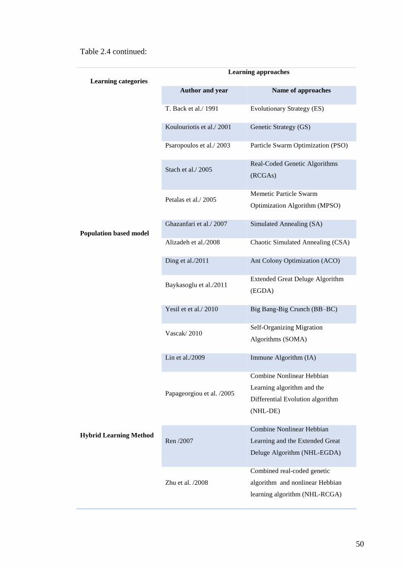
50
Table 2.4 continued:
Learning categories
Learning approaches
Author and year Name of approaches
Population based model
T. Back et al./ 1991 Evolutionary Strategy (ES)
Koulouriotis et al./ 2001 Genetic Strategy (GS)
Psaropoulos et al./ 2003 Particle Swarm Optimization (PSO)
Stach et al./ 2005 Real-Coded Genetic Algorithms
(RCGAs)
Petalas et al./ 2005 Memetic Particle Swarm
Optimization Algorithm (MPSO)
Ghazanfari et al./ 2007 Simulated Annealing (SA)
Alizadeh et al./2008 Chaotic Simulated Annealing (CSA)
Ding et al./2011 Ant Colony Optimization (ACO)
Baykasoglu et al./2011 Extended Great Deluge Algorithm
(EGDA)
Yesil et et al./ 2010 Big Bang-Big Crunch (BB–BC)
Vascak/ 2010 Self-Organizing Migration
Algorithms (SOMA)
Lin et al./2009 Immune Algorithm (IA)
Hybrid Learning Method
Papageorgiou et al. /2005
Combine Nonlinear Hebbian
Learning algorithm and the
Differential Evolution algorithm
(NHL-DE)
Ren /2007
Combine Nonlinear Hebbian
Learning and the Extended Great
Deluge Algorithm (NHL-EGDA)
Zhu et al. /2008
Combined real-coded genetic
algorithm and nonlinear Hebbian
learning algorithm (NHL-RCGA)

51
2.5 Summary
In this chapter, the fuel cell background is presented and in a brief review PEM fuel
cell history and basic principle are described. Various main types of fuel cells such as
electrochemical reaction are briefly explained. Currently, PEM fuel cell has a wide range
of applications and the focus of this research is on this type of fuel cell. Depending on
power capacity of fuel cell, the main applications are categorized into residential,
portable, stationary and transportation. For the commercialized PEM fuel cell, study on
improving efficiency and performance are the most serious challenges. In addition,
accurate modeling of PEM fuel cell for improving efficiency has been a topic of interest
for researchers in the last two decades. In this chapter a review of accurate recent models
was provided and linear regression (LR), artificial neural network (ANN) and fuzzy
cognitive map (FCM) are proposed for modelling the PEM fuel cell.

52
Chapter 3 : METHODOLOGY
3.1 Introduction
Based on the reviewed literature, modelling of complete electric vehicle with
auxiliary parts is essential to adjust the optimization ability. In addition, a reliable model
can benefit the system’s efficiency with proper control methods to optimize its
performance. Based on the problem statement, this study has multiple objectives: First, it
aims to define the precise value of the whole system efficiency as well as its correlation
with power and other affecting factors; second, it aims to design optimized linear and
non-linear dynamic models of the system in order to enable real-time prediction of voltage
and efficiency. Experimental data was collected by DAQ system from the electric bicycle;
then, efficiency of whole system was calculated based on the collected data. In the next
step, PEM fuel cell electric bicycle has been modelled by using both linear and non-linear
approaches. Linear regression model and neural network models were used to predict the
output voltage and efficiency. Finally, for the first time in this field, a dynamic fuzzy
cognitive map was designed to define the causality of system concepts for active
modeling of each system parameter. These steps are shown as a flowchart in Figure 3.1.

53
Figure 3.1: Methodology flow chart
Data collection
Linear
Regression
Load
Voltage
Fuzzy Cognitive
Map
(FCM)
Efficiency
Modelling
Evaluation
Real-time Fuzzy
Cognitive Map
modelling
Electric
bicycle
Oxygen
flow rate
Hydrogen
flow rate
Humidity
Temperature
Current
Non-Linear
Regression

54
3.2 PEM fuel cell system
Commercial electric bicycle and PEM fuel cell that have been installed in the system to
provide the power are described as follows:
3.2.1 Overall System Design (Electric Bicycle)
The commercial electric-assisted bicycle that we used in this research is shown in
Figure 3.2. As shown in the figure, the components of our system included a fuel cell
stack forming the base of the system and integrated with other major components to
generate electricity. Metal hybrid is used for storage of a large amount of hydrogen in
small tank in electric bicycle. Fuel cell powered the electric motor located in tier and
remote control to turn the fuel cell on and off.
Figure 3.2: Fuel cell-powered electric bicycle
Fuel
Cell
SysteRemote
Control
Metal Hybrid
storage tank Electric motor
Handlebar
throttle

55
3.2.2 PEM fuel cell powered bicycle
The block diagram of the fuel cell-powered electric bicycle is shown in Figure3.3.
The 𝐻2from a metal hydride tank and 𝑂2 from the air blower are fed to the fuel cell, where
they are combined to form water; a process that consequently produces electricity.
Figure3.3: Block diagram of the fuel cell-powered electric bicycle system
Figure3.4 shows a complete fuel cell system, which consists of the fuel cell, one
cooling and one reaction air blower, the Electronic Control Unit (ECU), and the necessary
auxiliaries to manage the hydrogen flow.
Battery
Valve
Metal h
yb
rid
M
oto
r
DC
DC
Control
Unit
Auxiliaries
Fuel
cell
Air blower

56
Figure3.4: Fuel Cell and auxiliary components
The entire system is controlled by an ECU designed by MES S.A., which monitors
all the system's parameters and operates the system on command. The ECU features an
accessible remote control outside of the main box, and the driver can switch the main
power on/off and start the fuel cell on demand. The ECU operates the fuel cell during the
start, normal operation, and shutdown procedures by monitoring various parameters such
as the stack temperature, hydrogen pressure, stack voltage, stack current, battery voltage,
and ambient condition. When the ECU detects an abnormal condition, it will alert the
driver via the LED indicators placed on the remote control and handlebar throttle. If the
condition for a security shut off (TRIP) is fulfilled and remains unchanged for a certain
security time, the system will shut off automatically.

57
3.3 Data collection and analysis
The DAQ system and its software were designed by MES S.A., and used serial
connection between Fuel Cell ECU and monitoring software. To connect the ECU and
PC, it is recommended to use (nine-pole) communication cable with this specification:
RS 232 (nine-pole), Pin to pin. The connector labelled ECU has to be connected to the
appropriate nine pole connector of the ECU, the connector labelled PC to a COM port of
the PC. As shown in Figure 3.5 all Fuel Cell parameters are monitored and can be logged.
Figure 3.5: The panel of monitoring software for fuel cell system
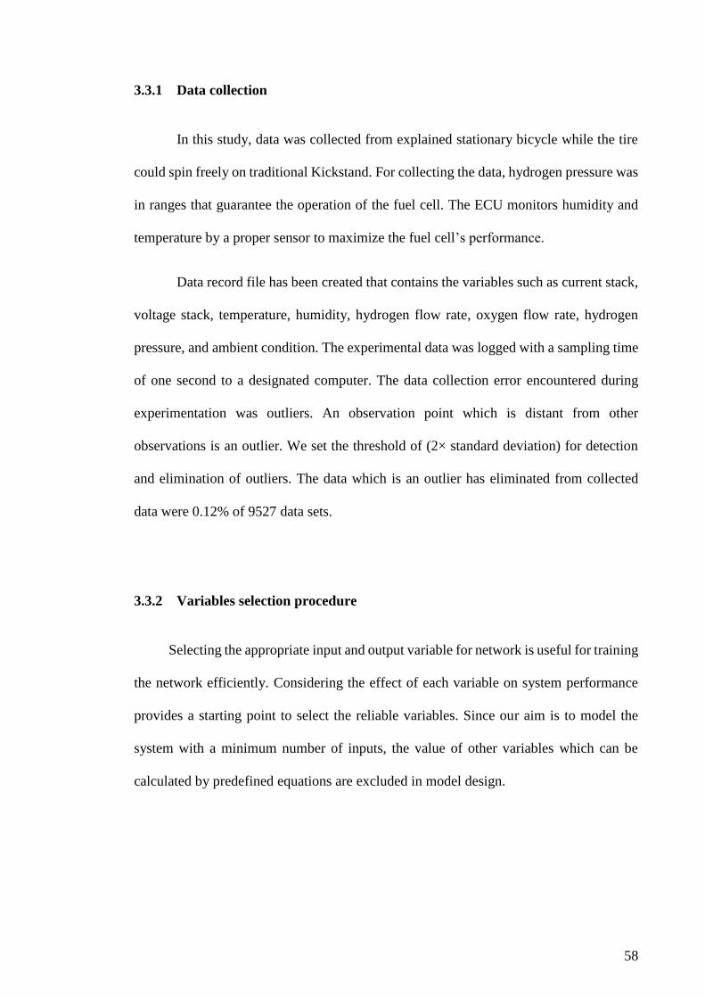
58
3.3.1 Data collection
In this study, data was collected from explained stationary bicycle while the tire
could spin freely on traditional Kickstand. For collecting the data, hydrogen pressure was
in ranges that guarantee the operation of the fuel cell. The ECU monitors humidity and
temperature by a proper sensor to maximize the fuel cell’s performance.
Data record file has been created that contains the variables such as current stack,
voltage stack, temperature, humidity, hydrogen flow rate, oxygen flow rate, hydrogen
pressure, and ambient condition. The experimental data was logged with a sampling time
of one second to a designated computer. The data collection error encountered during
experimentation was outliers. An observation point which is distant from other
observations is an outlier. We set the threshold of (2× standard deviation) for detection
and elimination of outliers. The data which is an outlier has eliminated from collected
data were 0.12% of 9527 data sets.
3.3.2 Variables selection procedure
Selecting the appropriate input and output variable for network is useful for training
the network efficiently. Considering the effect of each variable on system performance
provides a starting point to select the reliable variables. Since our aim is to model the
system with a minimum number of inputs, the value of other variables which can be
calculated by predefined equations are excluded in model design.

59
This project collected seven variables of electric bicycle performance information
including the stack temperature, ambient humidity, stack voltage, stack current, stack
power, hydrogen flow rate, and oxygen flow rate. The models use five inputs and two
outputs nodes.
3.4 Efficiency of fuel cell
Calculating the efficiency for the entire system is necessary in order to improve the
performance of the system. Previous studies focused more on analyzing the efficiency
and performance of single cell. The efficiency properties of the fuel cell stack and each
single cell are similar because all similar single cells are connected in series. Fuel cell
efficiency has been computed from the fuel cell's stack operating voltage (𝑉𝑜𝑝𝑒𝑟) using
the following equation (Feroldi & Basualdo, 2012):
ηfc% =
100% × Voper
1.482 × n
(3.1)
where n in number of cells, 𝜂𝑓𝑐 is fuel cell efficiency and 1.482 V corresponds to
the hydrogen higher heating value (HHV) (Feroldi & Basualdo, 2012). For hydrogen, the
HHV is used when the amount of released hydrogen heat energy is measured by cooling
its combustion vessel to 25 C (initial temperature of vessel). In contrast, 1.254 V is used
in equation (3.1), which corresponds to the lower heating value (LHV) when the vessel
cooling is halted at 150 ℃. The hydrogen LHV is used when the efficiency will be
compared to internal combustion engine for transportation. However, many researcher
reported fuel cell efficiencies using hydrogen HHV. Equation (3.1) cannot be used to
calculate the efficiency of the entire system because this formula provides the instant

60
efficiency of the stack that is proportional to the stack's voltage. The system's efficiency
during the experimental time is computed using the following equation:
ηfcsystem, % =
100% × generated electric energy
energy of cunsumed H2
(3.2)
The mass of the consumed hydrogen stored in a metal hydride tank for our
experiment is calculated using the ideal gas law because the bicycle tank had been directly
charged from a buffer tank of an electrolyzer system. The energy content of the hydrogen
LHV is 241.98 kJmol-1, or 120.1 MJkg-1. Hydrogen can release this energy via ignition
heat. Hence, the energy of consumed hydrogen for lower heat values is calculated using
the following equation:
Energy of consumed H2, kJ =
241.98 × ∆p × V
R × T
(3.3)
where ∆𝒑 is the pressure drop (atm) of the electrolyzer storage tank after charging
the bicycle metal hydride tank, V is the volume (L) of an electrolyzer buffer tank, T is the
temperature (K) of the buffer tank, and R is ideal gas constant, 0.08206 L atm mol-1 K-1.
Because 1W.h =3.6 kJ, the numerator of the equation (3.4) can be defined as follows:
Generated electric energy, kJ = 3.6 × ∑(V × I × ∆h) (3.4)
During the transfer of two electrons from water molecules in fuel cells, the ideal cell
voltage or standard potential to produce water in a liquid state (25 ℃, 1 atm) is 1.23 V,
while the voltage drops to nearly 1.18 V for producing water in gaseous state or at
operating temperatures exceeding approximately 80 ℃. Therefore, the theoretical or
maximum efficiency of fuel cell was calculated to be 83% and 94.1% for HHV and LHV,
respectively, by substituting the standard voltage in Equation (3.1).
Nevertheless, the experimental efficiency is expected to be lower than the
theoretical efficiency for emerging losses even without being connected to any external

61
load. Furthermore, the efficiency is expected to steeply decline when the load is connected
because the voltage drops due to inevitable losses generated by the electrical current in a
closed circuit. Furthermore, a fraction of the power generated by a primary fuel cell is
used by the required auxiliary components, which include the control unit, blowing fan,
cooling fan, and battery.
3.5 Data-set
The Data-set which was used for training and evaluation of the regression
algorithms consisted of 720 data points from different states of system. The data included
current, voltage, temperature, hydrogen flow rate, oxygen flow rate, related humidity and
efficiency. Based on the advanced machine learning consideration in accurate designing
of a regression model, 60% of the data was used for training, 20 % for cross-evaluation
and 20% for testing the algorithm. The exact number of dataset for training the algorithm
to obtain the highest accuracy in evaluation dataset was chosen based on information
extracted from the learning curve. Cross-validation and training data sets have been used
for optimizing the regression algorithm parameters. However, data-set was pre-processed
for better performance of the models.
Five variables have been used as inputs (current, hydrogen flow rate, oxygen flow
rate, temperature, related humidity) of regression models to predict voltage and efficiency
as desired system outputs.

62
3.5.1 Data normalization
In this system, parameter values varied in the range and their standard deviations.
Therefore, data was normalized to facilitate the training by providing a greater
homogeneity of the input and output variables. In order to normalize the data mean has
been calculated and consecutively standard variation of each variable has been computed
as:
𝑆 = √∑ (𝑥𝑖 − �̅�)2𝑛
𝑖=1
𝑛 − 1 (3.5)
Where n is number of random samples. The z-score of value x is computed by:
𝑧 =
𝑥 − �̅�
𝑆 (3.6)
Where x is the sample data with mean �̅� and standard deviation named S. Standardization
of data or z-score calculated the distance between raw data and mean in terms of standard
deviation. When the raw score is below the mean the sign of z-score is negative and is
positive when the score is above (Abdi, 2007).
3.5.2 Principle component analysis (PCA)
Processing time is one of the most essential factors in introducing reliable real-
time systems. Simplicity of the model as well as reducing the calculation needed are two
main affected factors which can be provided by reducing the dimensionality of input
variables. Principle component analysis (PCA) is a useful statistical technique for finding
patterns to reduce the dimension of data set and it is a powerful tool for data analysis
without losing more than 1% of data.

63
This section briefly describes the steps needed to perform PCA analysis on a set
of data. Figure 3.6 shows the parameters that apply to our model.
Step1: Get input data-set as an m × n matrix where number of measurements is
denoted by m and the number of trails by n.
Step2: Subtract the mean, which is the average across each dimension.
Step3: Compute the covariance matrix. For more details on covariance calculating
see (Smith, 2002).
Step4: Calculate the eigenvectors and eigenvalues of the covariance matrix based
on singular value decomposition algorithm. These calculations give us more information
about the data.
Step5: Choose the component and form a feature vector, which complies to the
concept of data compression and reduces dimensionality.
Step 6: Deriving the new data set, which is the final step in PCA
Figure 3.6: qH2: hydrogen flow, qO2: oxygen flow, I: current load T: temperature, H:
humidity
Pre
processing
qO2
I
H
T
qH2
PC2
PC1
PC3
Models V

64
PCA has been applied on input data (current, temperature, related humidity,
hydrogen flow rate and oxygen flow rate) only to reduce the complexity of calculations
and to decrease the processing time.
3.6 Regression models
Researchers predict the performance of fuel cell as a function of various operating
conditions by using empirical modelling. These models avoid identifying the knowledge
of process parameters which is difficult to determine from fuel cell system. Empirical
modelling of the system is based on setting measurable parameters and choosing
appropriate inputs for predicting the behaviour of interested outputs.
For an accurate modelling of the PEM fuel cell output voltage and system efficiency,
two approaches have been used in this study. First approach based on linear modelling
using linear regression algorithm. Artificial neural networks has been used for non-linear
modelling of the system as the second approach. In both models, related humidity (RH),
current (I), oxygen flow rate (qO2), temperature (T) and hydrogen flow rate (qH2) were
set as input variables and fuel cell voltage (v) and efficiency (eff) were the predicted
values. Collected data was randomly divided into three groups for training (60 %), cross
validation and test dataset. The remaining 40% of the data was randomly assigned into
two equal groups for cross-validation and test datasets accordingly. In both regression
models, advanced machine learning principles were considered for optimizing the designs
based on learning curve and error processing results as shown in Figure 3.7 (Perlich,
2011). The number of training data sets was chosen based on learning curve analysis and
cost function during the training procedure in order to overcome the high bias (under-
fitting) and high variance (over-fitting) problems.

65
3.6.1 Linear Regression
Classical linear regression method is most commonly used in linear modeling the
behavior of structural systems. Linear regression is a method for calculating the relation
between explanatory variable and depended variable by fitting the linear equation to the
observed data. Figure3.8 shows the basic linear regression model.
Output
𝐲𝐢
1
𝒙𝟐
Input
∑
𝒙𝟏
𝒙𝒏
Figure3.8: Linear regression configuration
Training set Test set
Training set Validation
set
Learn
models
Select
model
Learning process
Learned model
Regression
model
Artificial neural
network model
Figure 3.7: Flowchart depicts the training process of regression models. Training and
validation datasets were used for model training and optimization of model parameters.
Test data set was used for evaluation of final design

66
The multiple linear regression equation given 𝑛 features is denoted as:
ℎ𝜃(𝑥) = 𝜃0 + 𝜃1𝑥𝑖1 + 𝜃2𝑥𝑖2 + ⋯ + 𝜃𝑘𝑥𝑖𝑘 𝑓𝑜𝑟 𝑖 = 1,2, . . , 𝑛 (3.7)
where 𝑥 is explanatory variable, and ℎ𝜃(𝑥) is the predicted value (hypothesis),
𝜃0 is the intercepts, and 𝜃 is the estimated slope coefficient of the line.
By vectorising equation (3.5) we have:
The error term(𝜀) of this model is the difference between the real value (y) and the
predicted value (h) of equation (3.3) which is calculated by Mean squared Error (MSE)
of the difference between the predicted values and the actual value (hθ(xi)- yi ) as shown
in equation (3.4) which is referred to as the cost function 𝐽(𝜃):
𝑦 − ℎ𝜃(𝑥) = 𝜀 (3.9)
𝐽(𝜃) =
1
2𝑚∑(ℎ𝜃 (𝑥(𝑖)) − 𝑦(𝑖))
𝑚
𝑖=1
2
(3.10)
Where 𝑚 is the number of iterations and 𝐽(𝜃) is function of the parameter vector.
ℎ𝜃(𝑥) = 𝜃𝑇𝑥
𝜃 = [𝜃0, 𝜃1, … , 𝜃𝑛+1]
𝑥 = [𝑥0, 𝑥1, … , 𝑥𝑛+1]
While 𝑥0 = 1
(3.8)

67
The objective of linear regression is to estimate the unknown parameters while
cost function is minimum. To fulfill these requirements, a fundamental algorithm called
Gradient Descent (GD) is used as a promising method for estimating the interception
vector 𝜃 in order to minimize the cost function (MSE).
3.6.1.1 Gradient Descent
In this project, Gradient descent algorithm was used for updating the system
weights (𝜃 vector) to calculate our hypothesis automatically. In gradient descent
algorithm, each 𝜃 value is updated based on the derivation of cost function and a learning
rate value (𝛼).
The values are updated by assigning new value for 𝜃 using the previous values to achieve
a lower MSE:
𝜃𝑗: = 𝜃𝑗 − 𝛼𝜕
𝜕𝜃𝑗𝐽(𝜃)
= 𝜃𝑗 − 𝛼𝜕
𝜕𝜃𝑗
1
2𝑚∑ (ℎ𝜃 (𝑥(𝑖)) − 𝑦(𝑖)𝑚
𝑖=1 )2
= 𝜃𝑗 − 𝛼 ∑ (ℎ𝜃 (𝑥(𝑖)) − 𝑦(𝑖))𝑚𝑖=1 𝑥𝑗
𝑖
(3.11)
It is noteworthy that the updating of θj vector should be done simultaneously for
all 𝜃 in each step for j = 0, … n. This process would be continued until convergence of Y
and ℎ𝜃(𝑥), where m is the size of training set and the value of the training set data is
shown by 𝑥(𝑖) , 𝑦(𝑖).
As shown in Figure 3.9 GD moves the weights in order to decrease the derivation
of MSE function. The final values of theta are the actual weights of the prediction model.

68
3.6.1.2 Learning curve
In order to have the best possible prediction, training data was split into three
parts: training set, cross validation set and testing set. As a general rule, 60% of the sample
are training set and 20% for each of cross validation and test set. A learning curve is a
plot of the training and cross validation mean square error versus the index of the training
data set. These plots are useful to find better prediction of the system; i.e. how beneficial
it will be to add more data to training set. When both training set and cross validation set
are converging to a low value, there is no need to add more data to the training set.
Iteration 4
Convergence
Iteration 3
F(x)
x
Starting point
Final
value
Figure 3.9: Gradient decent

69
3.6.2 Artificial Neural Network (ANN)
For non-linear modeling of the system, artificial neural network (ANN), a
mathematical computation model introduced by McCulloch and Pitts in 1943, was used.
In the 1950’s, some development of neural network in both theory and practice occurred
(Braspenning, Thuijsman, & Weijters, 1995). Ability to learn from the input data with or
without teacher is one of the features of neural networks. Nonlinearity, adaptively, input
output mapping and fault tolerance are other important features. In ANN, can be defined
as computational tools which make the experimental knowledge to be available to be
used (Zilouchian & Jamshidi, 2000).
Currently, various fields of neural network applications have been developed such
as pattern recognition, time series analysis, signal processing, modelling and control. The
structure of artificial neural network neuron is based on a simple mathematical model of
the human brain.
3.6.2.1 The Neural Network Basic Architecture
Neural network consists of several neurons connected to perform a specific task.
A processing unit, as shown in Figure3.10, is the basic component of neural network. The
synaptic weight represents acquired knowledge that has been used to connect each input
to a neuron.

70
A nonlinear model of neuron’s output can be described as follows:
uk = ∑ wkjxj
m
j=1
(3.7)
Synaptic weights (wkj) are multiplied by each input (xm) in the neuron 𝑘, and the output
is computed as:
𝑣𝑘 = 𝑢𝑘 + 𝑏𝑘 (3.13)
The general model output of neuron shown by 𝑦𝑘, and 𝜑(. ) is the activation
function effected by bias for limiting the amplitude and defines the output of neuron
(Sablani, Datta, Rahman, & Mujumdar, 2006).
𝑦𝑘 = 𝜑(𝑢𝑘 + 𝑏𝑘) (3.148)
Output
𝐲𝐤
Synaptic weights
Summing
junction
Bias
bk
∑
𝒙𝟏 𝑤𝑘1
𝑤𝑘2
𝑤𝑘𝑚
𝒙𝟐
𝒙𝒎
Activation
function
𝒗𝒌
𝜑(. )
Figure3.10: Artificial Neuron configuration

71
3.6.2.2 Network Architecture
Learning algorithm and network architecture are two important factors for better
network training performance. The fundamental neural network architecture that we use
in this work is multiplayer feed-forward network.
The most popular neural network is multiplayer feed-forward network that has
one or more hidden layers. For extracting higher order of the network, one or more hidden
layer is added which might tend to smoothing the network output. As shown in
Figure 3.11 multiplayer feed-forward networks have one input, one or more hidden layer
and one output. In the input layer, neurons operate by receiving the signal from the user.
Through the connections, signals are moved to the hidden layer. In networks that have
more hidden layers, the input of the second hidden layer is the output of the first hidden
layer and so on. To produce the network output, the signals are transmitted to the output
(Sablani et al., 2006).
RH
Output
Input
Input
layer Hidden
layer
Output
layer
Figure 3.11: Multiplayer Feedforward Network, where I: current, H2: hydrogen flow
rate, O2: oxygen flow rate, RH: related humidity and T: temperature as an inputs and
V: voltage and EFF efficiency of system as an outputs
O2
H
2
I
T
Eff
V
Hidden
layer

72
Levenberg-Marquardt back propagation algorithm is a variation of Newton’s
method, which implies a simplified form of Hessian matrix applied to train the proposed
neural network model. The sum of square error is denoted by 𝐹(𝑥)and combination of
the weights matrix and bias is indicated by x. Hessian matrix 𝐻(𝑥) is described as follows
(Gavin, 2011).
𝐻(𝑥) = ∇2𝐹(𝑥) = 2𝐽𝑇(𝑥)𝐽(𝑥) (3.15)
The gradient g(x) can be calculated as:
𝑔(𝑥) = ∇𝐹(𝑥) = 2𝐽𝑇(𝑥)𝑣(𝑥) (3.16)
Where 𝑣(𝑥) is a vector of network error, and 𝐽(𝑥)is the Jacobian matrix
The LM-BP algorithm can be calculated by the following equation:
𝑥𝑘+1 = 𝑥𝑘 − [𝐽𝑇(𝑥𝑘)𝐽(𝑥𝑘) + 𝜇𝑘𝐼]−1𝐽𝑇(𝑥𝑘)𝑣(𝑥𝑘) (3.17)
Parameter 𝜇𝑘 is multiplied by some factor (𝜃) whenever a step increases 𝐹(𝑥). 𝜇𝑘
is divided by (𝜃) when a step is reduced 𝐹(𝑥) (the algorithm begins with 𝜇𝑘 set to a small
value, such as 𝜇𝑘 = 0.01and 𝜃 > 1). The algorithm becomes the steepest descent while
𝜇𝑘is large with step 1𝜇𝑘
⁄ and the algorithm becomes Gauss-Newton when 𝜇𝑘is small
which provides rapid convergence and procedures approximating Hessian matrix. For
effective agreement between the guaranteed convergence of the steepest descent method
and the speed of Newton’s method, LM-BP algorithm is used.

73
3.6.3 Fuzzy Cognitive Map:
Fuzzy cognitive map (FCM) introduced by Kosko in 1986 is a soft computing tool
based on fuzzy logic (FL) and neural network (NN) methodologies (Kosko, 1986; O.
Motlagh et al., 2012). FCM is classified as a neuro-fuzzy system which can easily
incorporate and adapt human knowledge and represent a given system with a set of
concepts and common relations between them. Inclusion of uncertainties is the one
promising feature of FCM which means when less knowledge about the variable is
available, no precise initial node weight is needed, and therefore FCM is more robust.
Currently, various areas of the fuzzy cognitive map applications such as medicine,
international relations, political science, history and engineering are being developed.
Relationship representation is the most significant improvement concern of
FCMs. This means instead of using only sign, the degree of considered casual relation is
associated with a number (weight) (Stach, Kurgan, & Pedrycz, 2005). The strength of
relationship is described by a number from [-1, 1] interval. Promoting effect is reflected
by positive values, while inhibiting effect corresponds to negative value. Value of +1
represents full positive, -1 corresponds to full negative, with neutral relation defined by
0. Other values are used for different fuzzy levels of casual effect.
As mentioned above, a FCM model is represented in the form of graphs. In a
graphical representation, set of nodes (concept, Ci) and their connection edges correspond
to causal effect relationships, represented by weights (Wij) between them. Three possible
types of causal relationships between concepts are expressed as follow: Wij > 0 indicates
positive causality between two concepts which means increasing the value of one concept
leads to increasing the value of the other concepts. Wij < 0 indicates negative effect

74
between two concepts which means increasing the value of one concept causes a decrease
in another concept. Wij = 0 means there is no relationship between the two concepts.
Model can be presented by a square matrix, which is known as connection matrix.
All values of edge weights between corresponding concepts are stored in rows and
columns of this matrix (Stach, Kurgan, Pedrycz, et al., 2005). Figure 3.12 shows a FCM
model and its connection matrix.
C1 C2 C3 C4 C5
C1 0 W2,1 W1,3 0 W1,5
C2 W2,1 0 0 0 0
C3 W3,1 0 0 0 0
C4 W4,1 0 0 0 0
C5 0 W5,2 0 W5,4 0
W1, 3
W3,1
W4,1
W1,5
W5,4 W5,2
W1,2
W2,1
C1
C4
C3
C5
C2
Figure 3.12: Example of FCM graph and corresponding connection matrix

75
Model can be simulated when the primary values of concepts have been
determined as primary state of whole system and consequently FCM has been created.
Simulation of the system’s dynamic is performed by functional modelling of FCM based
on equation (3.18):
∀ 𝑗 ∈ {1, … , 𝑁}, 𝐶𝑗(𝑡 + 1) = 𝑓 (𝐶𝑗(𝑡) + ∑ 𝑒𝑖𝑗𝐶𝑖(𝑡)
𝑁
𝑖=1
) (3.18)
where 𝐶𝑗(𝑡) is activation degree of concept 𝑗𝑡ℎ at time t, 𝑒𝑖𝑗 denotes the
relationship strength between concept 𝐶𝑖 with concept 𝐶𝑗 if 𝑖 ≠ 𝑗 and 𝑒𝑖𝑗 = 0 if 𝑖 = 𝑗,
and finally 𝑓 is transformation function comprised of the periodic relationship between
𝐶(𝑡 + 1) and 𝐶(𝑡) for 𝑡 ≥ 0 (Stach, Kurgan, & Pedrycz, 2005).
Starting point of simulation consists of computing initial values of the state vector
over a number of successive iterations. Present values of all nodes in specific iteration are
determined by state vector. Former iteration values of nodes which influence the given
node through cause-effect relationship are used to calculate the value of a given node.
Iterative application of the equation (3.18) leads to calculating successive states.
The transformation function is used to preserve the weighted sum within a certain
range normally set to [0, 1]. Quantitative analysis is lost by applying nonlinear
transformation function, but comparison of activation levels which can be defined as
active (value of 1), in active (value of 0) and active to a certain degree (value between 0
and 1). Some commonly used threshold functions are listed below:
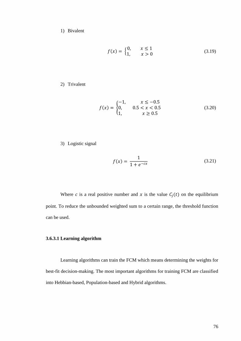
76
1) Bivalent
𝑓(𝑥) = {0, 𝑥 ≤ 11, 𝑥 > 0
(3.19)
2) Trivalent
𝑓(𝑥) = {
−1, 𝑥 ≤ −0.5 0, 0.5 < 𝑥 < 0.51, 𝑥 ≥ 0.5
(3.20)
3) Logistic signal
Where 𝑐 is a real positive number and 𝑥 is the value 𝐶𝑗(𝑡) on the equilibrium
point. To reduce the unbounded weighted sum to a certain range, the threshold function
can be used.
3.6.3.1 Learning algorithm
Learning algorithms can train the FCM which means determining the weights for
best-fit decision-making. The most important algorithms for training FCM are classified
into Hebbian-based, Population-based and Hybrid algorithms.
𝑓(𝑥) =
1
1 + 𝑒−𝑐𝑥 (3.21)

77
3.6.3.1.1 Hebbian learning algorithm
Hebbian based method updates the FCM weights based on Hebbian law and
available data. More successful weight matrices are then produced. Hebbian learning
algorithm increases the efficiency, flexibility and dynamic behavior of FCM model. For
training FCM the most efficient Hebbian based methods are the following:
3.6.3.1.2 Nonlinear Hebbian learning (NHL)
The NHL is based on the nonlinear Hebbian learning raw for training the FCM.
NHL is based on the assumption that at each iteration, all the concepts are triggered and
synchronously update their value. Initial FCM and values of concepts are taken by
learning algorithm, and until the desired map is defined, weights keep on being updated.
The values of other weights which remain zero do not change. During the learning process
the nodes which are directly connected are updated according to their physical
incorporation. For the entire learning process, the weight values retain their initial sign
and direction as suggested by experts.
For finding the weights of neuron Oja learning rule is introduced which can be
expressed as follows:
𝑒𝑖𝑗(𝑘) = 𝑒𝑖𝑗(𝑘 − 1) + 𝜂𝐶𝑗(𝐶𝑖 − 𝑠𝑔𝑛(𝑒𝑖𝑗)𝐶𝑗𝑒𝑖𝑗(𝑘 − 1)) (3.22)
Where 𝐶𝑖 𝑎𝑛𝑑 𝐶𝑗 are the current activation values of concept 𝑖𝑡ℎ 𝑎𝑛𝑑 𝑗𝑡ℎ
calculated for each iteration, 𝑒𝑖𝑗(𝑘) is the value of the weights between concepts
𝑖𝑡ℎ 𝑎𝑛𝑑 𝑗𝑡ℎand 𝜂 is the learning coefficient.

78
Hebbian learning principle is based on the premise that weights update 𝑒𝑖𝑗 and
the product of the 𝐶𝑖 and 𝐶𝑗 concept activation are proportional. However, this may lead
to infinite growth of the weight values. Oja learning rule uses forgetting term to avoid
this effect that is reduced by iteration. In this method, the forgetting term is proportional
to weight values and square of the value of target concepts (for𝑒𝑖𝑗, 𝐶𝑗 is the concept).
This method has two conditions. The first one is the Desired Output Concepts
(DOC) which utilizes information on desired value of some concepts and usually has
predefined desired values. For each specific problem, when all desired concepts reach or
become close enough to the desired activation level, the learning may be completed. The
second condition takes into consideration the variation of the subsequent values of the
DOCs and is held if all of them change less than a predefined very small constant e.
Algorithm stops the learning process when e is larger than the variation in DOCs.
3.6.3.1.3 Data-driven nonlinear Hebbian learning (DD-NHL)
The DD-NHL is based on an improved version of NHL principle and applied on
the historical data to train the model. For training fuzzy cognitive map, seven steps of
generic NHL and proposed novel approach of learning FCM which is called DD-
NHL(Stach et al., 2008) are described:
Non-linear Hebbian algorithm:
Step 1: 𝐶(0) 𝑘𝑛𝑜𝑤𝑛 𝑎𝑠 𝑣𝑎𝑙𝑢𝑒 𝑜𝑓 𝑐𝑜𝑛𝑐𝑒𝑝𝑡𝑠 and 𝐸(0) as the connection matrix
and restriction imposed on desired value of DOCs in form of 𝐶𝑗𝑀𝑖𝑛 ≤ 𝐶𝑗 ≤ 𝐶𝑗
𝑀𝑎𝑥
Step 2: For each iteration step k

79
Step 3: according to equation (3.22) update the weights
Step 4: according to equation (3.18) for each concept calculate 𝐶(𝑘)
Step 5: Evaluate termination condition using 𝐶(𝑘) from step 4, 𝐸(𝑘)and 𝐸(𝑘 −
1)
Step 6: When both termination conditions are fulfilled go to step 2
Step 7: Return the final connection matrix 𝑊𝐹𝐼𝑁𝐴𝐿
Two conditions from step 6 can be defined as follows:
Condition1: (minimize the cost function F) for each 𝑓 = √∑ ‖𝐶𝑗(𝑘) − 𝑇𝑗‖2
𝐷𝑂𝐶𝑗 where
𝑇𝑗 is the mean target value of the concept 𝐶𝑗 mean: 𝑇𝑗 =𝐶𝑗
𝑀𝑎𝑥−𝐶𝑗𝑀𝑖𝑛
2
Determining the set of weights is the objective of the training process that minimizes
function F.
Condition 2: (after limited number of steps, terminate the algorithm)
Step 1: Calculate the maximum difference 𝑒𝑚𝑎𝑥 between 𝑒𝑖𝑗(𝑘) and 𝑒𝑖𝑗(𝑘 − 1)
Step 2: Return “True” if the absolute value of 𝑒𝑚𝑎𝑥 is less than 𝜀, otherwise return
“False”.
Now assume that for the given system the historical data are available. Matrix D
is formed, where 𝑑𝑖𝑗 is related to the value of 𝑖𝑡ℎ concept at the 𝑗𝑡ℎ time point. In other
words, value of concepts is defined as time series. Size of matrix D is 𝐾 × 𝑁 where the
number of available data points is denoted by 𝐾 and the number of concepts in modeled
system is defined by 𝑁. Figure 3.13 shows the flowchart of NHL algorithm.

80
Produce the final
connection matrix
If emax< ε
and F
calculate
Calculate the
cost function
Calculate emax
between eij (k)
and eij (k-1)
For k=1 more
iteration
Update the
weights
Calculate C (k)
for each
concept
Set the initial
matrix
Start
Evaluate
termination
conditions
Figure 3.13: Flowchart of NHL

81
Available historical data in step 4 are used by data-driven nonlinear Hebbian
learning (DD-NHL) which is improved as the follows:
Step 4: Define 𝐶(𝑘) in accordance with the next row of matrix D.
Therefore, based on available data used in each iteration step, the matrix is updated. Same
data points are utilized when all data points are exploited and the termination conditions
are not satisfied. Essentially, Oja learning rules are used in DD-NHL, but for a given
system it takes advantage of the data available instead of creating the data used for
training only from the current model. Initial connection matrix is still needed in DD-NHL
but randomly generated initial map can be used instead of on expert generated map.
Until the stable state is obtained, from primary state vector, current FCM is
simulated after each iteration of updating the weights. Then, the value of DOCs from this
state and the desired value of DOCs, are compared. When the answer is found, this
technique guarantees it would meet all the learning conditions. Figure 3.14 displays the
flowchart of DD-NHL algorithm. Thus, condition 1 is defined as follows:
Condition 1: (checking condition imposed on DOCs)
Step 1: Until the fixed state is reached simulate the current FCM defined by 𝐸(𝑘)
starting from the initial condition 𝐶(0).
Step 2: For each 𝐶𝑗 that has been defined as 𝐷𝑂𝐶𝑗, check whether the fixed value
𝐶𝑗(𝑛) meets the constraint 𝐶𝑗𝑀𝑖𝑛 ≤ 𝐶𝑗(𝑛) ≤ 𝐶𝑗
𝑀𝑎𝑥
Step 3: Return “False” if there is at least one 𝐶𝑗 that does not meet the limitation
from step 2.
Step 4: otherwise return “True”.

82
Start
Simulate the
FCM
If fix state
is reached
For DOCj check that Cj(n)
meets the constraint
𝐶𝑗𝑀𝐼𝑁 ≤ 𝐶𝑗(𝑛) ≤ 𝐶𝑗
𝑀𝐴𝑋
At the least one
Cj(n) are not
met restriction
True
Figure 3.14: Flow chart of DD-NHL
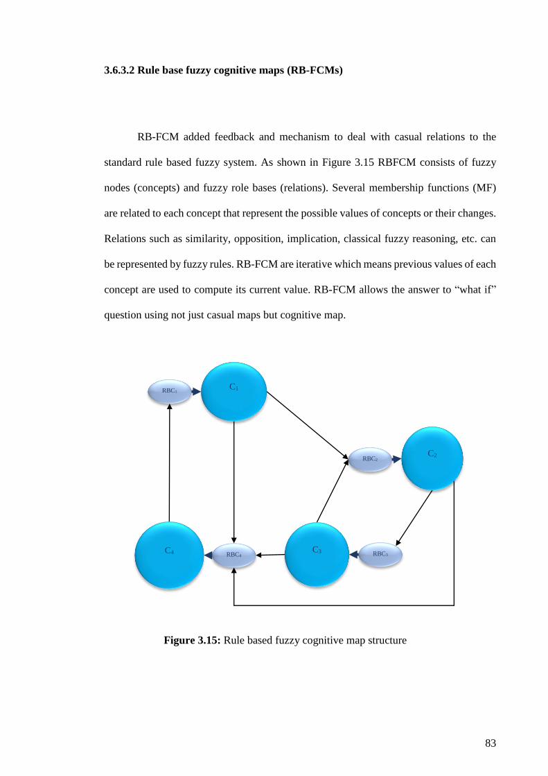
83
3.6.3.2 Rule base fuzzy cognitive maps (RB-FCMs)
RB-FCM added feedback and mechanism to deal with casual relations to the
standard rule based fuzzy system. As shown in Figure 3.15 RBFCM consists of fuzzy
nodes (concepts) and fuzzy role bases (relations). Several membership functions (MF)
are related to each concept that represent the possible values of concepts or their changes.
Relations such as similarity, opposition, implication, classical fuzzy reasoning, etc. can
be represented by fuzzy rules. RB-FCM are iterative which means previous values of each
concept are used to compute its current value. RB-FCM allows the answer to “what if”
question using not just casual maps but cognitive map.
C1
C2
C3 C4
RBC1
RBC2
RBC4 RBC3
Figure 3.15: Rule based fuzzy cognitive map structure

84
3.6.3.3 Linguistic variables influence for FCM weights
This methodology presented here makes fuzzy cognitive map structure closer to
fuzzy logic. The influence of concept Ci on concept Cj which has been determined by
experts as negative or positive and with linguistic variables describe the grade of influence
such as “strong”, “weak” and etc. The interval of linguistic variable, is [-1, 1] and its term
set T (influence) is suggested as: negatively very strong, negatively strong, negatively
medium, negatively weak, zero, positively weak, positively medium, positively strong,
positively very strong.
Figure 3.16 shows the membership function characterized by fuzzy sets. Semantic
rule M can be defined as follows:
M (negatively very strong): membership function 𝜇𝑛𝑣𝑠 describe fuzzy sets
for “an influence below to -75%”.
M (negatively strong): membership function 𝜇𝑛𝑠 describe fuzzy sets for
“an influence close to -75%”.
M (negatively medium): membership function 𝜇𝑛𝑚 describe fuzzy sets for
“an influence close to -50%”.
M (negatively weak): membership function 𝜇𝑛𝑤 describe fuzzy sets for
“an influence close to -25%”.

85
M (zero): membership function 𝜇𝑧 describe fuzzy sets for “an influence
close to 0”.
M (positively weak): membership function 𝜇𝑝𝑤 describe fuzzy sets for “an
influence close to 25%”.
M (positively medium): membership function 𝜇𝑝𝑚 describe fuzzy sets for
“an influence close to 50%”.
M (positively strong): membership function 𝜇𝑝𝑠 describe fuzzy sets for “an
influence close to 75%”.
M (positively very strong): membership function 𝜇𝑝𝑣𝑠 describe fuzzy sets
for “an influence above to 75%”.
1
0.5
𝜇𝑝𝑠 𝜇𝑝𝑚 𝜇𝑛𝑤 𝜇𝑛𝑣𝑠 𝜇𝑛𝑠 𝜇𝑛𝑚 𝜇𝑝𝑤 𝜇𝑧 𝜇𝑝𝑣𝑠
1 -1 0.25 0 -0.25 -0.75 0.75 0.50 -0.50
Figure 3.16: Membership function for influence of the linguistic variables

86
Each interconnection defined by linguistic variables are combined and the interval
of overall linguistic variables is transformed to [-1, 1]. A numerical weight for each
interconnection will be the outcome of the defuzzifier where the Centre of Gravity method
is used to produce these weights. Figure 3.17 display flowchart of linguistic variable
influence for FCM.
This chapter has provided an in-depth and detailed of linear regression and
artificial neural network modelling. Network architecture and learning algorithms of both
modelling approaches are described. In addition, the fuzzy cognitive map algorithm is
presented. The fuzzy membership function and linguistic variables of FCM are explained
as well.
Figure 3.17: Flowchart of linguistic variable influence for FCM
Sort the weights in
range [-1, 1] with 0.2
interval
Number of
Wij
Start
Decide on number of
membership function
Real-time data
acquisition
Real-time data
acquisition Control
Visualization

87
Chapter 4 : RESULTS AND DISCUSSION
4.1 Introduction
This study aims to develop a model and control strategy for electric bicycle
powered by PEM fuel cell to improve the efficiency and performance of system. In the
first phase of the study, efficiency of electric bicycle was computed as the main indicator
for PEM fuel cell system performance. In the second phase of the study the modelling
and performance analysis of PEM fuel cell electric bicycle system has been carried out.
This includes the study and utilizing linear and nonlinear regressions for predicting
overall PEM fuel cell efficiency and output voltage based on some fundamental variables
namely current, temperature, humidity, hydrogen flow rate and oxygen flow rate. Finally,
fuzzy cognitive maps were used for the first time in this field to design a dynamic FCM
model for convenient control of system and real-time casualty calculation model among
the system concepts (current, temperature, humidity, hydrogen flow rate, oxygen flow
rate, voltage and efficiency). The validation of the applied cognitive model has been
ensured by comparison with a set of experimental data extracted from electric bicycle
system regarding electrical performance. In the following section each stage of result
representation will be explored in detail.

88
4.2 Data collection
Data set was collected from electric bicycle powered by PEM fuel cell using DAQ
system and are logged with sampling time of 1s to a designated computer. The installed
fuel cell is a 250-W PEM fuel cell, which contains a 22 cell air-cooled stack that provides
a nominal stack voltage and current at 14 V and 20 A. It generates a peak power of 250
W to a 25-kg bicycle with a rated consumption of 3.5 normal litters of H2 per minute. The
specifications of the fuel cell is listed in Table 4-1.
Table 4-1: Nominal Fuel cell specifications
Parameter Supplier Finding
Number of single cells 22 22
Maximum total power output (W) About 250 About 180
Output voltage (V) 13-20 13-20
Nominal stack current (A) 20 (max 28) 18
Weight of the stack (kg) 0.7 0.7
Overall dimensions of the Fuel Cell system
(blowers Inc.) (mm3) approx.230×220×150 approx.230×220×150
Ambient temperature range (°C) >0 up to +35 >0 up to +35
Ambient relative humidity range (%)
(recommended) 30-80 50
Hydrogen supply nominal pressure (bar) 0.65 0.65
Hydrogen supply minimum flow rate
guaranteed (Nl/min) 3.5 3.5
Maximum purged hydrogen flow rate (Nl/min) 0.07 0.07

89
A 150-W electric motor drives the bicycle via the regulated voltage from DC/DC
converter, which is connected to a 13.2-20.2 V unregulated output voltage of the fuel cell.
The DC/DC convertor is 300-W convertor from Zahn Elect with efficiency of 92% (at
Vin=12 V, I out=8.4 A) and recommended input voltage of 10-20 V.
The motor is activated by a handle bar mounted throttle, just like on most
motorcycles or scooters. In the other words, this vehicle is to be operated on a power-on
demand basis; the electric motor is only engaged and operated manually using a throttle,
while the pedalling can be coupled with the motor in tough conditions, such as cycling
uphill.
Figure 4.1: Plot of the voltage‒current and power-current curves of
Fuel Cell stack at temperature average of 37.6 °C

90
For a better visualization and operation dimensions of the system an example of
V-I and P-I curves of PEM fuel cell system are shown in Figure 4.1 which have been
obtained at approximately in constant fuel cell temperature 37.6 ℃ and relative humidity
averaging 48.8%. This plot shows the changes in constant temperature and humidity
condition which illustrates the typical V-I behaviour; the voltage monotonically decreases
as the current increased. As the V-I curve shows, the pattern after the sharp voltage drop
of the start-up experiences a steady linear decline when the current is increased.
While the load circuit is open, the current is close to zero, and the stack voltage is
estimated to at least be close to the theoretical value. However, the voltage is often
considerably less when a fuel cell is utilized. The following key points are evident from
the graph of the cell voltage versus the current:
The open circuit voltage is less than the theoretical value
A sharp initial voltage decrease is anticipated
The voltage then decreases less rapidly and more linearly
In addition, the stack at higher power production or current density releases more heat
if the system design is imperfect; the overheating that occurs during tough working
situations can disturb the normal operation of system.
Figure 4.2 shows that the ECU can perfectly control the temperature of stack and keep it
almost constant. The humidity curve illustrates the humidity ratio of the input air.

91
4.3 System efficiency
To study the behaviour and compute the efficiency of such system, we decided to
study, test, and analyse the features of an electric-assisted bicycle that is powered by a
PEM fuel cell as a common and suitable type of power source for transportation systems.
The efficiency‒power curve of a fuel cell stack is shown in Figure 4.3. It is plotted
using equation 3.1 for hydrogen HHV. As expected, a maximum efficiency of the fuel
cell’s stack is available in the low power or current range, as the highest stack voltage is
expected at an open circuit. Accordingly, while the stack power or current is increased,
the efficiency will decrease. As previously mentioned, this characteristic is the opposite
of the efficiency curve over power in an internal combustion engine, rendering the fuel
cell superior in terms of city transportation, where at most only a small fraction of nominal
power is required.
Figure 4.2: Plot of Stack temperature and air humidity ratio versus current density of
Fuel Cell

92
In the next step, efficiency of the whole system was analysed. As explained in
chapter 3, the ratio between the energy output and input forms the basis of calculation of
efficiency in any energy transformation system. This ratio in fuel cell is between the
output electrical power and the hydrogen energy that is consumed. The consumed
hydrogen energy for this experiment is calculated by Equation (3.3), as follows:
Energy of consumed H2 =241.98×4.96×20/ (308.65×0.08206) =947.75 kJ
Where for 3.92 mol of hydrogen, the pressure of 20-liter electrolyzer buffer tank was
dropped from 19.91 bar to 14.88 bar. Thus, 947.75 kJ was used by the fuel cell as the
system input, and the electric motor used the FC power output. The output electric power
of the system is calculated by measuring the power consumption of the bicycle’s electric
Figure 4.3: Plot of FC stack efficiency versus FC stack output power for relatively
average temperature 37.6 ℃ over experiment period

93
motor over time, which is 335.82 kJ, over approximately 159 minutes of experimental
period. Hence, the overall system efficiency for this experiment is calculated using
Equation (3.2):
The overall system efficiency =100×335.82/947.75=35.43 %
Figure 4.4 shows the Sankey diagram, which visualizes the different energy flows
and power losses in an analysed electric-bicycle system. As shown in the picture the entire
amount of hydrogen energy is 947.75 kJ and only 335.82 KJ is used for motor electric
power.
Hydrogen input
(947.75 kJ)
Motor electrical power
(335.82 kJ)
611.93
kJ
Electrical power
used by auxiliary
components
Heat
Figure 4.4: Flow diagram for PEM fuel cell powered electric bicycle.
This diagram illustrates the various energy flows in system

94
However, the following important point should be considered that the efficiency
of the fuel cell stack is not constant and depends on the stack voltage (bicycle usage
condition). Thus, this value can change for different experimental conditions for the same
bicycle. For this experiment, we have attempted to keep the bicycle at the cruise condition
(constant speed) with a fuel cell power average of 35.29 W, and fuel cell stack efficiency
average of 48.45%. The specifications of our efficiency study are listed in Table 4-2.
Table 4-2: Fuel cell powered electric bicycle parameter measurements from data
demonstrated in Figure 4.5 (efficiency indicted by eff)
Figure 4.5 shows the plot of the fuel cell power output throughout the efficiency
experiment. As the curve shows, we attempted to keep the output power constant for small
fractions of the nominal fuel cell power as needed at the cruise condition. The logged
power data in this curve show a bold line at the bottom of the power line. The power
differences between these higher points on top of this line and the points on the line are
due to auxiliaries, such as 10-W cooling blower, which the ECU altered to maintain its
Parameters Experiment
duration
Hydrogen
consumptiona
Load energy
consumptionb
System
effc
Max– Min
of FC effd
Mean
of FC
eff e
Mean of
FC
powerf
Value 9515 s
3.917 mol
(947.75 kJ)
335.82 kJ 35.43%
63.88%
42.69%
48.45 % 35.29
W
a From Equation (3.3)
b Consumption electric power obtained from the sum of 9515 load power values that logged each
second.
c Efficiency of fuel cell powered electric bicycle base on experimental data using Equation (3.2).
d The maximum and minimum of fuel cell stack efficiency during this experiment.
e Average of FC stack efficiency over 9515 individual efficiency values calculated for each second of
experimental time.
f The mean was calculated from 9515 individual data points shown in Figure 4.5

95
speed and compensate for the temperature of the fuel cell at the designated working
temperature. When the fan is working at a minimum rate, the load power and other
constant auxiliaries form the bold line in the curve, and the other variable components
form the approximately 15-W line.
Figure 4.5: Plot of fuel cell stack power measured during efficiency experiment
During the experiment, it was observed that the ECU always automatically shuts
down the system prior to reaching the full output power, which is important to the
performance. Data analysis shows that the fuel cell stack voltage is below the minimum
value (12 V) before reaching the maximum power due to insufficient hydrogen flow at
stack; therefore, the ECU automatically shuts down the system to protect the fuel cell.
As mentioned, the temperature of Metal Hydride tank decreases during de-charging,
the canister's surface temperature dropped from 27 ℃ to 0 ℃ in less than 15 min and this

96
affects the maximum hydrogen flow rate, which could potentially provide energy for fuel
cell. In other words, when the fuel cell of bicycle works for a while, Metal Hydride tank
cannot supply the minimum 3.5 Nl/ min of hydrogen in the time of high power demand
of bicycle. Consequently, the voltage of fuel cell drops under the limitation and ECU
shuts down the stack. Empirical model provides useful and reasonable accurate input-
output relations for finding better performance of system and prevents any danger in real
life for considering critical situations and investigating the system in various conditions.
In this section the results of modelling are considered.
4.4 System modelling
Empirical models provide useful and reasonable accurate input-output relations in
order to better investigate the system in various conditions to avoid any danger in real life
considering the critical situation. In this study, both linear and nonlinear regression
models were used for prediction of voltage and efficiency of system. In this section, the
results of each of these designs are reported.
For the purpose of system modelling, 720 data points of following variables have
been used. The data set collected from 25-kg electric bicycle powered by PEM fuel cell
for prediction of electric bicycle system included load current, temperature, humidity,
hydrogen flow rate, oxygen flow rate as regression model inputs and voltage and
efficiency as outputs. Classical Linear regression with gradient descent algorithm was
used for linear modelling, while a 3-layer feed forward artificial neural network with
Levenberg-Marquardt algorithm used for training.

97
4.4.1 Linear regression model
Based on the machine learning principles, 60 % of dataset has been used for
training while another 40% was divided equally into both cross-validation and test
datasets. Gradient descent algorithm is applied for training the data. Cross validation
dataset is used for model evaluation from splitting data set into training set for training
the classifier and validation set for evaluating the model and estimating the error rate of
trained classifier.
Cost function of training data set for both voltage and efficiency is shown in
Figure 4.6 which shows the Mean Squared Error (MSE) over 300 data points for training
for voltage and efficiency observed as 0.0302 and 0.106 respectively. To evaluate the
performance of PEM fuel cell linear regression model against experimental result, and in
order to find this performance numerically, mean squared error is necessary to be
calculated by the equation (4.1):
𝑀𝑆𝐸 =
1
𝑛∑(𝐴 − 𝑇)2
𝑛
𝑖=1
(4.1)
Where 𝐴 denotes the simulated data vector for every output parameter, T represents the
real experimental value.

98
Figure 4.6: MSE for training the data a) voltage b) efficiency
b)
a)

99
In this study, principles of machine learning were considered for an optimized
regression model design; therefore, learning curve based on training and cross-validation
sets have been manipulated to process the error of the model and modification of model
parameters using MSE. This evaluation was explained in chapter 3 and the best number
of data points for model training was set to 300 in order to make sure there is no
overtraining.
The performance of the linear regression model for the output voltage and
efficiency value are shown in Figure 4.7. The convergence of training and cross validation
error for 300 data points in the learning curve plots confirmed the optimal number of
training needed for this model. Cross validation has been used for model evaluation by
splitting the data set into training set for training the classifier and validation set for
evaluating the model and estimating the error rate of the trained classifier.

100
a)
b)
Figure 4.7: Training of linear regression model for output
a) voltage value b) efficiency value

101
To train the linear regression efficiently, selecting the number of variables as
inputs and outputs is useful. Evaluation of system performance based on selecting the
fewest dominate input variables can provide the fastest training, reduce unnecessary
complications and improve instant recall. In our particular system, as shown in Figure 4.8,
3 inputs were selected to the appropriate for modelling to avoid long run-time to achieve
results.
Once the model parameters were defined, a new random set of data were used for
final design and evaluation of regression model using test dataset. Once satisfactory
output has been provided by linear regression on the validation data set, cross validation
was carried out on the test set. After the final test, linear regression model used be ready
to predict V-I performance for different range of conditions.
Figure 4.8: Evaluation of system performance based on input features
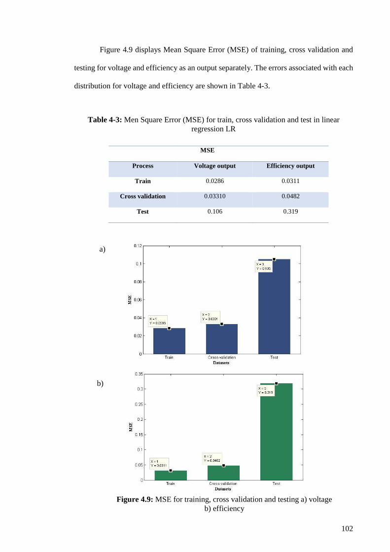
102
Figure 4.9 displays Mean Square Error (MSE) of training, cross validation and
testing for voltage and efficiency as an output separately. The errors associated with each
distribution for voltage and efficiency are shown in Table 4-3.
Table 4-3: Men Square Error (MSE) for train, cross validation and test in linear
regression LR
MSE
Process Voltage output Efficiency output
Train 0.0286 0.0311
Cross validation 0.03310 0.0482
Test 0.106 0.319
b)
a)
Figure 4.9: MSE for training, cross validation and testing a) voltage
b) efficiency

103
Designed linear regression model was used for prediction of voltage and
efficiency of test data and Figure 4.10 represents the sequence of simulated and real
output data voltage and efficiency for PEM fuel cell.
a)
b)
Figure 4.10: Comparison of predicted result and experimental data, a) voltage
simulation b) efficiency simulation by LR

104
Figure 4.11a) demonstrates the polarization curve predicted by the proposed linear
regression model. Representing the system behaviour with the smallest number of sensors
in electric bicycle as perfectly as possible by the proposed model, is one of the main
objectives here. In addition, Figure 4.11 b) represents the efficiency versus power curve
prediction.
Figure 4.11: Predict the a) polarization curve and b) efficiency versus power by
linear regression (LR) and compare with experimental data of PEM fuel cell.
a)
b)

105
4.4.2 Artificial neural networks model
Non-linear relations among numerous inner fuel cell parameters cause
nonlinearity functions for the whole system. Therefore, in order to have a non-linear
regression model for this electric bicycle, artificial neural network (ANN) have been
adopted. We investigated linear regression model and neural network model to determine
which one tends to provide better prediction in terms of accuracy and speed. Before
designing the network, a few dominate input and output variables are recognized.
To accelerate the performance prediction, it is important that training data set
goes through the normalization procedure and to be well distributed in operating range.
For training the NN, the inputs and outputs had to be normalized to be within a [-1, 1] for
better convergence of the model. Input features were reduced using the same principle
of linear regression by using first 3 principle components. Network was trained with
Levenberg-Marquardt back propagation (LM-BP) to produce the proper output. Scheme
neural network are shown in Figure 4.12.
Figure 4.12: Scheme of function fitting NN model

106
For selecting the best structure of neural network model, possible different hidden
layers and neuron structures have been designed and evaluated based on the MSE value
of the cross-validation set. Table 4-4 indicates that LM-BP with two layer 17-4 neurons
provided the best prediction in terms of accuracy and speed. Therefore, similar neuron
networks may perform better than complicated ones.
Number of epochs and the average error of prediction indicated by cost function,
which is calculated by equation below, determine the training speed:
costfunction =1
N∑ (DCi
estimated𝑁𝑖=1 − DCi
real)2 (4.2)
costfunction =1
N.(K−1)∑ ∑ (DCi
estimatedNj=1
K−1K=1 − DCi
real)2 (4.3)
Where N is the sample number. The error has been calculated by comparing real
values against estimated values for voltage and efficiency in the validation set.
Table 4-4: Prediction result for different network architectures
Hidden layer Epoch MSE Processing Time
3 10 0.074 00:00:17
3-3 74 0.055 00:00:18
10 70 0.044 00:00:01
10-10 12 0.071 00:00:00
20 12 0.035 00:00:00
20-10 11 0.134 00:00:01

107
Figure 4.13 displays the performance of the training, testing and validation
processes for output voltage variable. Critical convergence for best validation
performance is set to 10-2. After training the model for 10 epochs for voltage output and
16 epochs for efficiency output, the mean square error for voltage and efficiency is
observed to be 0.0118 and 0.0314 respectively. Table 4-5 demonstrates the best neural
network model performance with the higher correlation coefficient which has 17-4 hidden
neurons.
Figure 4.13: Best validation performance of neural network model for output
a) voltage and b) efficiency value
a)
b
)

108
Table 4-5: Performance of the best PEM fuel cell neural network model
Figure 4.14 displays the error histogram of the output variables. As shown, the
majority of error rates are in the interval of [-0.1, 0.2] and the error signal for training,
testing and validation is stretched out to the value of 0.8 for voltage and 0.9 for efficiency
outputs and the main portion lies between [-0.3, 0.4] and [-0.3, 0.4] for voltage and
efficiency output respectively.
Variable Mean square error Correlation coefficient
Tes
t
Load Voltage 0.0118 0.993
Efficiency 0.0314 0.982
Figure 4.14: Histogram of error for a) voltage output b) efficiency output
b)
a
)

109
For investigating the correlation between experimental data and predicted data
from ANN model, linear regression model of training, testing and validation set for every
output has been calculated. The training session for output voltage presented better
correlation rate which is R= 0.989 as shown in Figure 4.15 a) where the output efficiency
obtained the minimum correlation rate which is R= 0.977 (Figure 4.15 b))
Figure 4.15: Rates of correlation of output variables a)
voltage b) efficiency by linear regression for training
a)
b)

110
In order to provide accurate regression model, sufficient number of iterations
should be used in training phase. As shown in Figure 4.16 this procedure demonstrated
great behaviour. Figure 4.16 displays voltage variable obtained correlation rate of R=
0.993 and also shows that for efficiency variable R= 0.978
Figure 4.16: Correlation rate for testing patterns of outputs variable
a) voltage b) efficiency
a)
b)

111
In order to detect and compare predicted results against experimental results,
current sequence, temperature, humidity, hydrogen flow rate and oxygen flow rate were
propagated through the neural network model. Figure 4.17 displays outstanding
modelling performance of the neural network prediction, where estimated validation
pattern by data, show great linear fit to real data. Figure 4.17 a) demonstrates the
acceptable validation correlation rate of voltage in this procedure for R= 0.986 and
Figure 4.17 b) displays suitable performance of efficiency variable for R= 0.976.
a)
b)
Figure 4.17: Correlation rate of output variable a) voltage
b) efficiency for validation
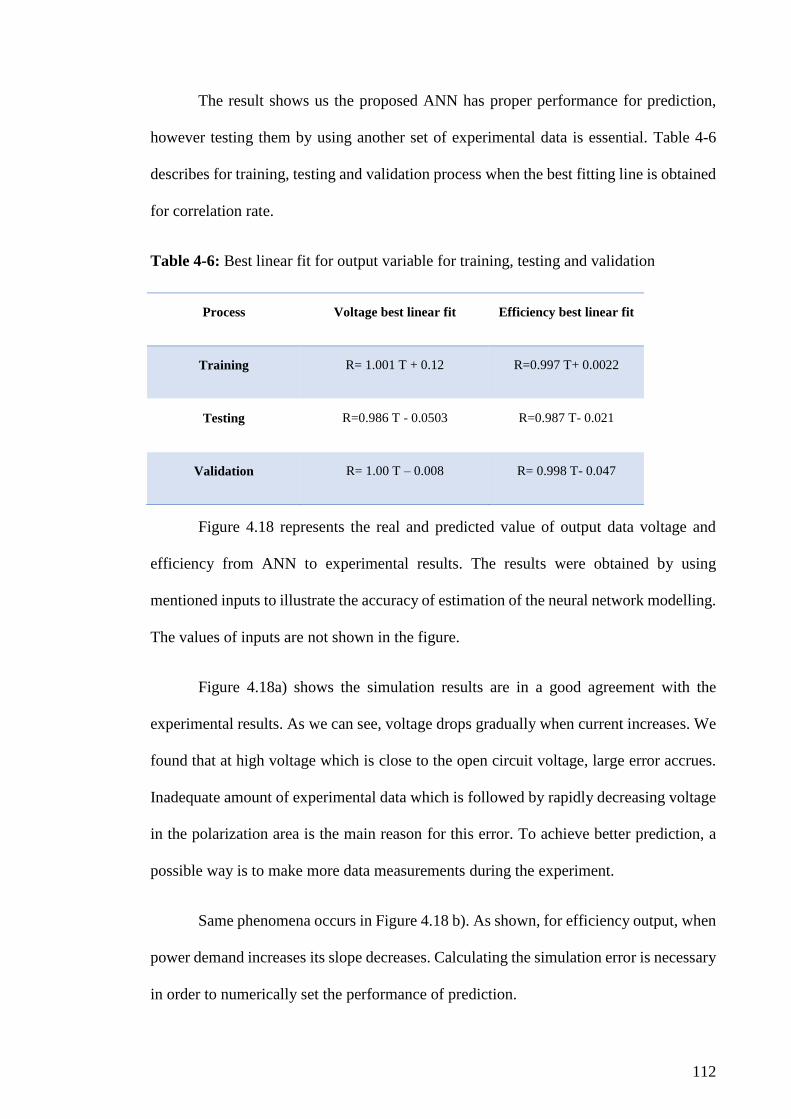
112
The result shows us the proposed ANN has proper performance for prediction,
however testing them by using another set of experimental data is essential. Table 4-6
describes for training, testing and validation process when the best fitting line is obtained
for correlation rate.
Table 4-6: Best linear fit for output variable for training, testing and validation
Figure 4.18 represents the real and predicted value of output data voltage and
efficiency from ANN to experimental results. The results were obtained by using
mentioned inputs to illustrate the accuracy of estimation of the neural network modelling.
The values of inputs are not shown in the figure.
Figure 4.18a) shows the simulation results are in a good agreement with the
experimental results. As we can see, voltage drops gradually when current increases. We
found that at high voltage which is close to the open circuit voltage, large error accrues.
Inadequate amount of experimental data which is followed by rapidly decreasing voltage
in the polarization area is the main reason for this error. To achieve better prediction, a
possible way is to make more data measurements during the experiment.
Same phenomena occurs in Figure 4.18 b). As shown, for efficiency output, when
power demand increases its slope decreases. Calculating the simulation error is necessary
in order to numerically set the performance of prediction.
Process Voltage best linear fit Efficiency best linear fit
Training R= 1.001 T + 0.12 R=0.997 T+ 0.0022
Testing R=0.986 T - 0.0503 R=0.987 T- 0.021
Validation R= 1.00 T – 0.008 R= 0.998 T- 0.047
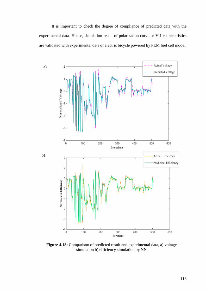
113
It is important to check the degree of compliance of predicted data with the
experimental data. Hence, simulation result of polarization curve or V-I characteristics
are validated with experimental data of electric bicycle powered by PEM fuel cell model.
Figure 4.18: Comparison of predicted result and experimental data, a) voltage
simulation b) efficiency simulation by NN
a)
b)

114
The comparison is demonstrated in Figure 4.19. The dataset used for this curve
prediction is the same as what we used in section 4.2. It is seen that as the current is
increased, the output voltage is decreased. The operated voltage is less than theoretical
due to various losses. It must be noted that the value of individual voltage losses inside
the PEM fuel cell cannot be computed by neural network model. Only general change in
voltage losses can be determined by the system’s model. We observe from the graph that
ANN gives fairly good prediction on voltage and current curves.
Figure 4.19: Prediction of the polarization curve by NN and comparison with
experimental data of PEM fuel cell

115
Figure 4.20 shows the simulation of efficiency versus power characteristics by
neural network. It can be noticed that maximum power is predicted close to the (17A)
fuel cell current which is similar to the experimental data.
As it can be seen in Table 4.7 comparison of the mean square error (MSE) for
voltage and efficiency as an output for regression and artificial neural networks are
displayed and ANN has had much better results.
Table 4.7 : Comparison MSE in artificial neural network (ANN) and
linear regression (LR) model
ANN LR
MSE Voltage Efficiency Voltage Efficiency
Train 0.0203 0.0334 0.0286 0.0311
Cross validation 0.0118 0.0443 0.03310 0.0482
Test 0.0203 0.0334 0.106 0.319
Figure 4.20: Prediction of efficiency versus power curve by NN and
comparison with experimental data of PEM fuel cell

116
4.5 Fuzzy Cognitive Map
As demonstrated earlier in chapter 2 and 3, fuzzy cognitive map (FCM) is a type
of network for describing the behaviour of systems in terms of concepts and effect
between concepts. In this study, measured variables were the concepts of FCM
(Figure 4.21) which consist of 7 concepts (C1=current, C2=temperature, C3=related
humidity, C4=hydrogen flow rate, C5= oxygen flow rate, C6=voltage, C7=efficiency). We
described the features of the system which are crucial for modelling and represented each
one by a concept.
The characteristics of PEM fuel cell system are demonstrated by the concepts
effects. The influence of the concepts on each other are represented by weights Wij among
them. In general, the key factor of PEM fuel cell system are represented by concepts that
can also be characteristics of the variables, inputs, outputs, events, states and trend of our
system. The weights between concepts are shown in matrix W (Table 4-8) as the initial
FCM of the PEMFC. As explained in chapter 3, any inner slope of self-effect of concepts
was considered as zero which caused the diagonal values of W matrix to be equal to zero.
The initial design of FCM with all weights consists of 42 connections among the
concepts. However, due to complexity the initial FCM is not shown in this thesis. Source
nodes are denoted by the rows of the matrix and destination nodes are denoted by the
columns. The concepts that influence other concepts are “Transmitter” and the concepts
influenced by other concepts are “Receiver”.

117
Table 4-8: FCM connection matrix between 7 concepts of PEM fuel cell system
I T RH H2 O2 V Eff
I 0 W1,2 W1,3 W1,4 W1,5 W1,6 W1,7
T W2,1 0 W2,3 W2,4 W2,5 W2,6 W2,7
RH W3,1 W3,2 0 W3,4 W3,5 W3,6 W3,7
H2 W4,1 W4,2 W4,3 0 W4,5 W4,6 W4,7
O2 W5,1 W5,2 W5,3 W5,4 0 W5,6 W5,7
V W6,1 W6,2 W6,3 W6,4 W6,5 0 W6,7
Eff W7,1 W7,2 W7,3 W7,4 W7,5 W7,6 0
We describe the relation between concepts by using a fuzzy value for each
interconnection, so weights take values in the interval [-1, 1]. As we mentioned in
chapter3, in FCM structure with three possible types of interaction between concepts
𝐶𝑖 and 𝐶𝑗 can be expressed as follows:
Wij > 0 specifies positive causality between two concepts which means
increase in the value of concept 𝐶𝑖 causes an increase in the value of concept 𝐶𝑗 and
decrease in the value of concept 𝐶𝑖 causes a decrease in the value of concept 𝐶𝑗 .
Wij < 0 indicates negative causality between two concepts that means
increase in the value of concept 𝐶𝑖 causes a decrease in the value of concept 𝐶𝑗 and vice
versa.
Wij = 0 indicates no relationship between two concepts.
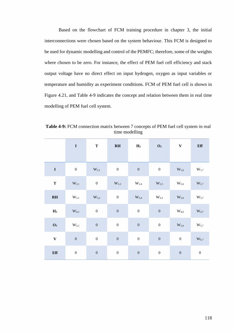
118
Based on the flowchart of FCM training procedure in chapter 3, the initial
interconnections were chosen based on the system behaviour. This FCM is designed to
be used for dynamic modelling and control of the PEMFC; therefore, some of the weights
where chosen to be zero. For instance, the effect of PEM fuel cell efficiency and stack
output voltage have no direct effect on input hydrogen, oxygen as input variables or
temperature and humidity as experiment conditions. FCM of PEM fuel cell is shown in
Figure 4.21, and Table 4-9 indicates the concept and relation between them in real time
modelling of PEM fuel cell system.
Table 4-9: FCM connection matrix between 7 concepts of PEM fuel cell system in real
time modelling
I T RH H2 O2 V Eff
I 0 W2,1 0 0 0 W1,6 W1,7
T W2,1 0 W2,3 W2,4 W2,5 W2,6 W2,7
RH W3,1 W3,2 0 W3,4 W3,5 W3,6 W3,7
H2 W4,1 0 0 0 0 W4,6 W4,7
O2 W5,1 0 0 0 0 W5,6 W5,7
V 0 0 0 0 0 0 W6,7
Eff 0 0 0 0 0 0 0

119
4.5.1 FCM Training Process
In this study, FCM has been used as a newly applied method for dynamic
modelling of the system, which can generate the next state of the whole system’s
concepts. This is the first dynamic model of a PEMFC, which predicts all variables
(concepts) of the system. To date, FCM has been used in many engineering applications,
and as one of the novelties of this study, FCM has been used for modelling PEMFC. It is
notable that there have been different algorithms designed for training FCM. However,
majority of these methods are based on an initial weight setting of FCM by an expert.
W5,6
W5,7 W5,1
W3,7
W2,6
W4,6
W4,7
W4,1
W2,6
W2,7
W2,5 W2,4
W3,4
W3,5
W3,6
W3,1
W6,7
W1,7
W1,6
W3,2
W2,3
W1,2
W2,1
I
T
RH
H2 O2
V
Eff
C1
C2
C3
C4
C5
C6
C7
Figure 4.21: FCM scheme of PEM fuel cell system, I: current, T: temperature,
RH: related humidity, H2: hydrogen flow rate, O2: oxygen flow rate, V: voltage
and Eff: efficiency
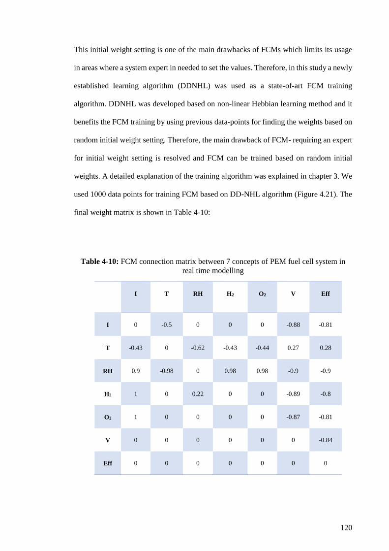
120
This initial weight setting is one of the main drawbacks of FCMs which limits its usage
in areas where a system expert in needed to set the values. Therefore, in this study a newly
established learning algorithm (DDNHL) was used as a state-of-art FCM training
algorithm. DDNHL was developed based on non-linear Hebbian learning method and it
benefits the FCM training by using previous data-points for finding the weights based on
random initial weight setting. Therefore, the main drawback of FCM- requiring an expert
for initial weight setting is resolved and FCM can be trained based on random initial
weights. A detailed explanation of the training algorithm was explained in chapter 3. We
used 1000 data points for training FCM based on DD-NHL algorithm (Figure 4.21). The
final weight matrix is shown in Table 4-10:
Table 4-10: FCM connection matrix between 7 concepts of PEM fuel cell system in
real time modelling
I T RH H2 O2 V Eff
I 0 -0.5 0 0 0 -0.88 -0.81
T -0.43 0 -0.62 -0.43 -0.44 0.27 0.28
RH 0.9 -0.98 0 0.98 0.98 -0.9 -0.9
H2 1 0 0.22 0 0 -0.89 -0.8
O2 1 0 0 0 0 -0.87 -0.81
V 0 0 0 0 0 0 -0.84
Eff 0 0 0 0 0 0 0

121
Based on the results of this step and in order to simplify the FCM of our system, residual
causalities and system concepts that are less effective were omitted from the final design
and Figure 4.22 was suggested for a new weight training. This simplification increases
the speed of FCM performance for each state prediction. The fuzzy cognitive model for
electric bicycle contains four concept including:
Concept 1 (C1): represents hydrogen flow rate (H2)
Concept 2 (C2): represents temperature
Concept 3 (C3): represents related humidity
Concept 4 (C4): represents efficiency of the system
The state-of-the-art learning method that exist in the literature is used for the investigation
of the quality of trained models. DD-NHL has been implemented to train this FCM model.
The simulation error was computed as follows:
Figure 4.22: Final FCM design of system.
-0.2 -0.5
C2 C1
C3
0.2
-0.03 0.56
0.01
0.26
0.22
T H2
RH
Eff
-0.8
C4

122
Where 𝐷𝐶𝑖𝑒𝑠𝑡𝑖𝑚𝑎𝑡𝑒𝑑 and 𝐷𝐶𝑖
𝑟𝑒𝑎𝑙 are the estimated and real value of decision concepts
(DC), 𝐾 is the number of available iterations to compare and 𝑁is the number of concepts
(E. I. Papageorgiou, 2013). By equation (4.3) the cost function is calculated:
In this condition our model can calculate the prediction error (which is the
summation of MSE for all concepts), while using it for improving its accuracy. The cost
function in FCM model as can be seen in Figure 4.23 is 0.0357.
𝑠𝑖𝑚𝑢𝑙𝑎𝑡𝑖𝑜𝑛_𝑒𝑟𝑟𝑜𝑟 =1
𝑁. (𝐾 − 1)∑ ∑| 𝐷𝐶𝑖
𝑒𝑠𝑡𝑖𝑚𝑎𝑡𝑒𝑑 − 𝐷𝐶𝑖𝑟𝑒𝑎𝑙|
𝑁
𝑗=1
𝐾−1
𝐾=1
(4.2)
𝑐𝑜𝑠𝑡_𝑓𝑢𝑛𝑐𝑡𝑖𝑜𝑛 =1
𝑁. (𝐾 − 1)∑ ∑(𝐷𝐶𝑖
𝑒𝑠𝑡𝑖𝑚𝑎𝑡𝑒𝑑
𝑁
𝑗=1
𝐾−1
𝐾=1
− 𝐷𝐶𝑖𝑟𝑒𝑎𝑙)2 (4.3)
Figure 4.23: MSE for training the data in FCM

123
The final values of W matrix is shown In Table 4-11, and the cost function
is depicted in Figure 4.23. This FCM MSE value is lower than the MSE for efficiency
and output voltage models that guarantee the highest accuracy on system modelling using
FCM.
Table 4-11: FCM connection matrix between four concepts of PEMFC
H2 T RH Eff
H2 0 0.2 0.22 -0.8
T 0.26 0 -0.03 -0.2
RH 0.56 0.01 0 -0.5
Eff 0 0 0 0
4.5.2 RB-FCM
Prediction model for precision PEM fuel cell system is developed by proposed
FCM approach that can be implemented for decision-making to control the system.
Figure 4.24 shows the corresponding membership function for the four selected
parameters (temperature, related humidity, hydrogen flow rate, and system efficiency).
Table 4-12 describes the set of linguistic variables that every concepts can take.

124
Table 4-12: Type of value of FCM Concepts
Type of value
Parameter Very low low Medium High Very high
Hydrogen flow
rate <-0.2 -0.2, 0 0, 025 0.25, 0.5 >0.5
Temperature <-0.4 -0.4, -0.20 -0.20, 0.20 0.2, 0.6 >0.6
Related
humidity <-0.4 -0.4, -0.15 -0.15, 0.25 0.25, 0.55 >0.55
Efficiency of
system <-2 -2, -1 -1, 0 0, 1.5 >1.5
Figure 4.24: Membership function for a) hydrogen flow rate b) Temperature
c) Related Humidity d) Efficiency
a)
d)
c)
b)

125
As explained in chapter 3, we use a rule-based FCM in this study which converts
the quantitative matrix weight into qualitative values which can be understood and
interpreted by any user. This benefits the system for a real time control and modification.
Using these fuzzy rules, the final weight matrix was converted to rule based FCM (RB-
FCM). Therefore, each concept value and the causality (influence matrix) should be
converted to fuzzy values. Figure 4.24 shows the fuzzy values for each concept. It is
notable that all the values of concept were normalized between [-1, 1] and based on the
density function of each concept, the fuzzy memberships were defined. In Figure 4.25the
membership function of influence matrix (W) is shown.
The influence of concept Ci to concept Cj is determined as negative or positive
and linguistic variables describe the grade of influence such as “strong”, “weak” and etc.
The interval of linguistic variable is [-1, 1] and its term set T (influence) are suggested as:
negatively very strong, negatively strong, negatively medium, negatively weak, zero,
positively weak, positively medium, positively strong, and positively very strong. Rule
M can be defined as follows:
M (negatively very strong): 𝜇𝑛𝑣𝑠 for “an influence below -0.85”.
M (negatively strong): 𝜇𝑛𝑠 for “an influence between -0.65 to 0.85”.
M (negatively medium): 𝜇𝑛𝑚 for “an influence in interval -0.45 to -0.65”.
M (negatively weak): 𝜇𝑛𝑤 for “an influence between -0.25 to – 0.45”.
M (zero): 𝜇𝑧 for “an influence between -0.2to 0.2”.

126
M (positively weak): 𝜇𝑝𝑤 d for “an influence between 0.2 to 0.45”.
M (positively medium): 𝜇𝑝𝑚 d for “an influence between 0.45 to 0.65”.
M (positively strong): 𝜇𝑝𝑠 s for “an influence between 0.65 to 0.85”.
M (positively very strong): 𝜇𝑝𝑣𝑠 for “an influence above to 0.85”.
Using these fuzzy rules, the final weight matrix was converted to rule-based FCM
(RB-FCM).
Figure 4.25: Membership function for influence matrix in electric bicycle
system

127
Figure 4.26 indicates Rule- Based FCM model. Relationship between a numbers of nodes
is determined by RB-FCM. For computing the new state of one node, fuzzy rules and
Defuzzification process were used.
In this section, a practical example of modelling the electric bicycle will be
examined. As mentioned before, the definition of concepts which describe the system and
relation between concepts are the most important components in developing FCM.
For electric bicycle system a fuzzy cognitive map with four concepts that gives a
good description of system is developed.
…
C1 C3
IF C1 is low THEN C2 is
very low
Defuzzification
IF C1 is high THEN C2
is medium
IF C1 is very high THEN
C2 is high
C1 C3 C2
RB-FCM relationship
Figure 4.26: Sample of RB-FCM relationship

128
Concept 1 Hydrogen flow rate
Concept 2 Temperature
Concept 3 Related humidity
Concept 4 Efficiency
These concepts are connected with each other. First, we decided about connection
between two concepts. Then, we decided the sign of connection, and at last, the weights
between connections were determined. Each event or connection between concepts has
weights that range in the interval [-1, 1]. The value of each concept has a range between
[-1, 1].
Now the connection between concepts are as follow:
Event 1 concept1 (hydrogen flow rate) connects with concept2
(temperature).
Event2 concept1 (hydrogen flow rate) relates with concept3 (related
humidity).
Event3 concept1 (hydrogen flow rate) connects with concept4
(efficiency).
Event4 concept2 (temperature) related with concept1 (hydrogen flow
rate).
Event5 concept2 (temperature) connects with concept3 (related humidity).
Event6 concept3 (related humidity) related with concept1 (hydrogen flow
rate).
Event7 concept3 (related humidity) connects with concept2 (temperature).

129
In this work, the relation among concepts has been described and to justify the
cause and effect of the relation between concepts, we have used IF-THEN rules, and also
for each interconnection, we have come up with the linguistic weight. The relation
between two concepts emerge as the weights of interconnection, are described by IF-
THEN rules. An example of fuzzy rule is as follows, where A, B, C are the linguistic
variables:
If an A change occurs in the value of concept Ci then a B change is caused in the value of
concept Cj. Thus, influence of concept Ci to concept Cj is C.
For every interconnection, we can propose linguistic rules; for the relationship
between two concepts, linguistic value can be concluded from the rules. Therefore, a
fuzzy rule has described the causal relationship that gives the degree of causality among
concepts and so the corresponding weights is derived. As an example, the relation
between two concepts will be examined (Figure 4.27).
If-then rule: If a very low change in value of concept Ci then a very high change in value
of concept Cj is caused.
Conclusion: The influence of Ci to Cj is positively very high and so value of Wij is
positively very strong.

130
To describe the relation between concepts RB-FCM used linguistic fuzzy rules
and they are not limited to casual relations. Now fuzzy if _then rules for each membership
function in the input concepts are defined by RB_FCM.
Rule 1: IF value of concept C1 (hydrogen flow rate) is very high THEN
value of concept C4 (efficiency) is low.
Inference: The influence of C1 to C4 is negatively strong, so value of Wij is
negatively strong.
Rule 2: IF value of concept C2 (temperature) is low THEN value of
concept C4 (efficiency) is medium.
Inference: The influence of C2 to C4 is negatively weak, so value of Wij is
negatively weak.
1
1
Wij
Positively very high
Influence
1
1
Ci
Very low
1
1
Cj
Very high
Figure 4.27: Example of fuzzy rule for an interconnection

131
Rule 3: IF value of concept C3 (related humidity) is high THEN value of
concept C4 (efficiency) is low.
Inference: The influence of C3 to C4 is negatively medium, so value of Wij is
negatively medium.
Rule 4: IF value of concept C1 (hydrogen flow rate) is very low THEN
value of concept C3 (related humidity) is low.
Inference: The influence of C1 to C3 is positively weak, so value of Wij is
positively weak.
According to the results achieved from voltage and efficiency equation shown in
chapter3 in the final system design, where it can be used for online control, voltage as a
system output was removed from FCM due to linearly correlation with efficiency and we
just put the concepts that can be controlled on alternative designs. It is noteworthy that
the design on Figure 4.21 also can be used, since capability of control system is feasible
only by some of the variables in the system which are suitable for real-time control such
as temperature, related humidity, hydrogen flow rate and efficiency (Figure 4.22). In
fuzzy cognitive map which describe the system, designer can easily decide to add or
remove connections. Moreover, for improving the system description and analyses of the
system performance in different conditions, concept can be added or removed, without
the reconstruction in whole model of the system. Since the initial design of the system is
done by extracting information from the system itself, this system can be controlled by
any operator without expert knowledge.

132
Chapter 5 : CONCLUSION AND FUTURE WORK
5.1 Conclusion
In this thesis, we described and experimentally tested a commercial electric
bicycle powered by a PEM fuel cell to investigate its performance and efficiency in real-
life operations. The polarization curve was obtained by using logged experimental data.
The stack voltage rapidly declined during the start-up of the system due to the losses,
which have strongly influenced later stages. The stack voltage also subtly reduces while
the current increases. This finding proves that improving the stack behaviour during start
up ameliorates the efficiency in future fuel cells. Furthermore, the overall system
efficiency was measured throughout normal daily life operations. The results demonstrate
that similar to internal combustion engines, the efficiency of the fuel cell is not a single
value and directly depends on the output power of the system.
However, the efficiency-power curves of fuel cells and internal combustion engines
showed opposite behaviours. The fuel cell-powered systems are more efficient at lower
output powers, which is the exact inverse of the behaviour of internal combustion engines.
The overall system efficiency was calculated to be approximately 35% for close to
cruising operations, while the stack efficiency varied 43-64% which is significantly
higher than that of an internal-combustion engine and also in compare to other similar
research which efficiency of 18.8-38% was recorded to be acceptable.
Consequently, any improvement in the system's performance to amend the efficiency
could lead to the growth of the fuel cell systems in transportation. For instance, adding a
regenerative break system to future designs can significantly increase the system's

133
efficiency, which could also save up to 28% of energy in a similar project involving
electric buses.
This study has evaluated modelling and controlling the PEM fuel cell system
using soft computing methodology including linear regression (LR) and artificial neural
network (ANN) methods. For model a PEM fuel cell system using related humidity (RH),
current (I), oxygen flow rate (qO2), temperature (T) and hydrogen flow rate (qH2) as the
input factors and fuel cell voltage (V) and efficiency (E) as the model output. Although
linear regression model has good results in predicting stack voltage, it was shown that
neural networks are more accurate and reliable for predicting fuel cell performance.
Neural networks are faster than other methods, including linear regression because they
are global approximators that operate without the need for any formula. In our research
work, for estimation of fuel cell stack voltage, an ANN model was used to predict the
commercial electric bicycle powered by PEM fuel cell that was trained by the Levenberg–
Marquardt back Propagation (LM-BP) algorithm.
The proposed model is easy to use and computationally fast. Result of the analysis
shows that the neural network algorithm fits the validation sample better than the linear
regression model. In addition, using the neural network technique the nonlinear variances
fit automatically, while linear regression techniques require an explicit design.
In the last part of this study, a new soft computing approach based on fuzzy
cognitive map (FCM) was proposed for the first time to describe the behaviour of electric
bicycle system powered by fuel cell. For automated learning of FCM from data, data
driven nonlinear hebbian learning (DD-NHL) is proposed. Then fuzzy rules explain the
cause and effect between concepts. Displaying the whole system behaviour by analytical
model is extremely difficult. Thus, it is more useful and attractive to consider system
behaviour in graphical way to show the causal relationship between concepts. One of the

134
superior capabilities of FCM is rule-based fuzzy cognitive map (RB-FCM) potential.
Since RB-FCM were developed to allow us to predict and analyse the cognitive map
involved in negotiation process. The main feature of RB-FCM are improving immunity
and stability to initial state, and flexible casual relation.
5.2 Contributions
This work has novel approaches in the following aspects:
We are experimentally compute the actual electric bicycle system's efficiency
Regression models were optimized for predicting the output variables (voltage
and efficiency).
FCM as a novel combination of fuzzy logic (FL) and neural network (NN)
approaches was utilized for the first time in this field. The novelty of this model
make it possible to predict the whole system variables.
This approach can be further developed to allow control this system in different
condition
5.3 Future work
Based on the research work in my dissertation regarding a two-wheel fuel cell
system have motivated me to a further research in modelling and nonlinear controlling
design related to fuel cell system and other renewable energy systems. The potential for
future work on fuel cell vehicle design will be proposed in the following directions:
Any improvement in the system's performance to amend the efficiency could lead
to the growth of the fuel cell systems in transportation. For instance, adding a
regenerative break system to future designs can significantly increase the system's

135
efficiency, which could also save up to 28% of energy in a similar project
involving electric buses.
A prediction algorithm with more variables can be considered in future work to
increase the accuracy of the model.
This thesis has presented some rules for decision-making to control the electric
bicycle; in terms of higher-level optimization of electric bicycle efficiency and
increase the lifetime of component. The corresponding controller can be designed
in future.

136
References
Abdi, H. (2007). Z-scores. Encyclopedia of measurement and statistics. Thousand Oaks, CA: Sage.
Acampora, G., & Loia, V. (2009). A dynamical cognitive multi-agent system for enhancing ambient intelligence scenarios. Paper presented at the Fuzzy Systems, 2009. FUZZ-IEEE 2009. IEEE International Conference on.
Acampora, G., Loia, V., & Vitiello, A. (2011). Distributing emotional services in ambient intelligence through cognitive agents. Service Oriented Computing and Applications, 5(1), 17-35.
Aguilar, J. (2003). A dynamic fuzzy-cognitive-map approach based on random neural networks. International Journal of Computational Cognition, 1(4), 91-107.
Andreou, A., Mateou, N. H., & Zombanakis, G. A. (2003). The Cyprus puzzle and the Greek-Turkish arms race: Forecasting developments using genetically evolved fuzzy cognitive maps. Defence and Peace Economics, 14(4), 293-310.
Andreou, A. S., Mateou, N. H., & Zombanakis, G. A. (2005). Soft computing for crisis management and political decision making: the use of genetically evolved fuzzy cognitive maps. Soft Computing, 9(3), 194-210.
Asl, S. S., Rowshanzamir, S., & Eikani, M. (2010). Modelling and simulation of the steady-state and dynamic behaviour of a PEM fuel cell. Energy, 35(4), 1633-1646.
Azmy, A. M., & Erlich, I. (2005). Online optimal management of PEM fuel cells using neural networks. Ieee Transactions on Power Delivery, 20(2), 1051-1058. doi: 10.1109/tpwrd.2004.833893
Azmy, A. M., & Erlich, I. (2005). Online optimal management of PEMFuel cells using neural networks. Power Delivery, IEEE Transactions on, 20(2), 1051-1058.
Bagotsky, V. S. (2012). Phosphoric Acid Fuel Cells. Fuel Cells: Problems and Solutions, Second Edition, 99-106.
Barbir, F. (2012). PEM fuel cells: theory and practice: Academic Press.
Barbir, F., & Gomez, T. (1996). Efficiency and economics of proton exchange membrane (PEM) fuel cells. International Journal of Hydrogen Energy, 21(10), 891-901.

137
Barbir, F., & Gomez, T. (1997). Efficiency and economics of proton exchange membrane (PEM) fuel cells. International Journal of Hydrogen Energy, 22(10-11), 1027-1037. doi: Doi 10.1016/S0360-3199(96)00175-9
Baschuk, J. J., & Li, X. G. (2005). A general formulation for a mathematical PEM fuel cell model. Journal of Power Sources, 142(1-2), 134-153. doi: 10.1016/j.jpowsour.2004.09.027
Baschuk, J. J., & Li, X. H. (2000). Modelling of polymer electrolyte membrane fuel cells with variable degrees of water flooding. Journal of Power Sources, 86(1-2), 181-196. doi: 10.1016/s0378-7753(99)00426-7
Beeson, P., Modayil, J., & Kuipers, B. (2009). Factoring the mapping problem: Mobile robot map-building in the Hybrid Spatial Semantic Hierarachy. The International Journal of Robotics Research.
Bhagavatula, Y. S., Bhagavatula, M. T., & Dhathathreyan, K. (2012). Application of artificial neural network in performance prediction of PEM fuel cell. International Journal of Energy Research, 36(13), 1215-1225.
Bischoff, M., & Huppmann, G. (2002). Operating experience with a 250 kWel molten carbonate fuel cell (MCFC) power plant. Journal of Power Sources, 105(2), 216-221. doi: http://dx.doi.org/10.1016/S0378-7753(01)00942-9
Blomen, L. J., & Mugerwa, M. N. (2013). Fuel cell systems: Springer Science & Business Media.
Boscaino, V., Miceli, R., & Capponi, G. (2013). MATLAB-based simulator of a 5 kW fuel cell for power electronics design. International Journal of Hydrogen Energy, 38(19), 7924-7934. doi: 10.1016/j.ijhydene.2013.04.123
Bossel, U., Schönbein, C. F., & Grove, W. R. (2000). The Birth of the Fuel Cell: 1835-1845. Including the First Publication of the Complete Correspondence from 1839 to 1868 Between Christian Friedrich Schoenbein (discoverer of the Fuel Cell Effect) and William Robert Grove (inventor of the Fuel Cell).
Boutalis, Y., Kottas, T. L., & Christodoulou, M. (2009). Adaptive estimation of fuzzy cognitive maps with proven stability and parameter convergence. Fuzzy Systems, IEEE Transactions on, 17(4), 874-889.
Brandon, C., & Hommann, K. (1996). The Cost of Inaction: Valuing the Economy-wide Cost of Environmental Degration in India: UNU, Institute of Advanced Studies.
Braspenning, P. J., Thuijsman, F., & Weijters, A. J. M. M. (1995). Artificial neural networks: an introduction to ANN theory and practice (Vol. 931): Springer Science & Business Media.

138
Buchholz, M., & Krebs, V. (2007). Dynamic modelling of a polymer electrolyte membrane fuel cell stack by nonlinear system identification. Fuel Cells, 7(5), 392-401.
Cai, Y., Miao, C., Tan, A.-H., Shen, Z., & Li, B. (2010). Creating an immersive game world with evolutionary fuzzy cognitive maps. IEEE computer graphics and applications(2), 58-70.
Carvalho, J. P. (2010). On the semantics and the use of fuzzy cognitive maps in social sciences. Paper presented at the Fuzzy Systems (FUZZ), 2010 IEEE International Conference on.
Carvalho, J. P., & Tomè, J. A. (1999). Rule based fuzzy cognitive maps-fuzzy causal relations. Computational Intelligence for Modelling, Control and Automation, Edited by M. Mohammadian.
Ceraolo, M., Miulli, C., & Pozio, A. (2003). Modelling static and dynamic behaviour of proton exchange membrane fuel cells on the basis of electro-chemical description. Journal of Power Sources, 113(1), 131-144. doi: 10.1016/s0378-7753(02)00565-7
Chang, K.-Y., & Teng, Y.-W. (2012). THE OPTIMAL DESIGN FOR PEMFC MODELING BASED ON BPNN AND TAGUCHI METHOD. International Journal of Green Energy, 9(2), 139-159. doi: 10.1080/15435075.2011.622018
Chang, W.-Y. (2013). Equivalent Circuit Parameters Estimation for PEM Fuel Cell Using RBF Neural Network and Enhanced Particle Swarm Optimization. Mathematical Problems in Engineering. doi: 10.1155/2013/672681
Chávez-Ramírez, A. U., Muñoz-Guerrero, R., Duron-Torres, S., Ferraro, M., Brunaccini, G., Sergi, F., . . . Arriaga, L. (2010). High power fuel cell simulator based on artificial neural network. International Journal of Hydrogen Energy, 35(21), 12125-12133.
Chavez-Ramirez, A. U., Munoz-Guerrero, R., Duron-Torres, S. M., Ferraro, M., Brunaccini, G., Sergi, F., . . . Arriaga, L. G. (2010). High power fuel cell simulator based on artificial neural network. International Journal of Hydrogen Energy, 35(21), 12125-12133. doi: 10.1016/j.ijhydene.2009.09.071
Chen, H.-W., Hsaio, H.-C., & Wu, S.-J. (1992). Current Situation and Prospects of Motorcycle Pollution Control in Taiwan, Republic of China: SAE Technical Paper.
Cheng, S.-J., Miao, J.-M., & Wu, S.-J. (2013). Use of metamodeling optimal approach promotes the performance of proton exchange membrane fuel cell (PEMFC). Applied Energy, 105, 161-169.
Chunying, Z., Lu, L., Dong, O., & Ruitao, L. (2011). Research of rough cognitive map model Advanced Research on Electronic Commerce, Web Application, and Communication (pp. 224-229): Springer.

139
Contreras, A., Posso, F., & Guervos, E. (2010). Modelling and simulation of the utilization of a PEM fuel cell in the rural sector of Venezuela. Applied Energy, 87(4), 1376-1385. doi: 10.1016/j.apenergy.2009.05.040
Cook, B. (2002). Introduction to fuel cells and hydrogen technology. Engineering Science & Education Journal, 11(6), 205-216.
Dickerson, J., & Kosko, B. (1993). Virtual worlds as fuzzy cognitive maps. Paper presented at the Virtual Reality Annual International Symposium, 1993., 1993 IEEE.
Dicks, A. L. (2004). Molten carbonate fuel cells. Current Opinion in Solid State and Materials Science, 8(5), 379-383.
Dockery, D. W., Pope, C. A., Xu, X., Spengler, J. D., Ware, J. H., Fay, M. E., . . . Speizer, F. E. (1993). An association between air pollution and mortality in six US cities. New England journal of medicine, 329(24), 1753-1759.
Dyer, C. K. (2002). Fuel cells for portable applications. Journal of Power Sources, 106(1), 31-34.
Faiz, A., Weaver, C. S., & Walsh, M. P. (1996). Air pollution from motor vehicles: standards and technologies for controlling emissions: World Bank Publications.
Ferng, Y., Tzang, Y., Pei, B., Sun, C., & Su, A. (2004). Analytical and experimental investigations of a proton exchange membrane fuel cell. International Journal of Hydrogen Energy, 29(4), 381-391.
Feroldi, D., & Basualdo, M. (2012). Description of PEM fuel cells system PEM Fuel Cells with Bio-Ethanol Processor Systems (pp. 49-72): Springer.
Fuerte, A., Valenzuela, R. X., & Daza, L. (2007). Preparation and characterisation of SOFC anodic materials based on Ce–Cu. Journal of Power Sources, 169(1), 47-52. doi: http://dx.doi.org/10.1016/j.jpowsour.2007.03.033
Funes, E., Allouche, Y., Beltrán, G., & Jiménez, A. (2015). A Review: Artificial Neural Networks as Tool for Control Food Industry Process. Journal of Sensor Technology, 5(01), 28.
Furfaro, R., Kargel, J. S., Lunine, J. I., Fink, W., & Bishop, M. P. (2010). Identification of cryovolcanism on Titan using fuzzy cognitive maps. Planetary and Space Science, 58(5), 761-779.
Furht, B., & Marques, O. (2003). Handbook of video databases: design and applications: CRC press.

140
Garche, J., Dyer, C. K., Moseley, P. T., Ogumi, Z., Rand, D. A., & Scrosati, B. (2013). Encyclopedia of electrochemical power sources: Newnes.
Gavin, H. (2011). The Levenberg-Marquardt method for nonlinear least squares curve-fitting problems. Department of Civil and Environmental Engineering, Duke University, 1-15.
Georgopoulos, V. C., Malandraki, G. A., & Stylios, C. D. (2003). A fuzzy cognitive map approach to differential diagnosis of specific language impairment. Artificial Intelligence in Medicine, 29(3), 261-278. doi: http://dx.doi.org/10.1016/S0933-3657(02)00076-3
Gong, W., & Cai, Z. (2014). Parameter optimization of PEMFC model with improved multi-strategy adaptive differential evolution. Engineering Applications of Artificial Intelligence, 27, 28-40. doi: 10.1016/j.engappai.2013.07.016
Gonzalez, J. L., Aguilar, L. T., & Castillo, O. (2009). A cognitive map and fuzzy inference engine model for online design and self fine‐tuning of fuzzy logic controllers. International Journal of Intelligent Systems, 24(11), 1134-1173.
Haji, S. (2011). Analytical modeling of PEM fuel cell i-V curve. Renewable Energy, 36(2), 451-458. doi: 10.1016/j.renene.2010.07.007
Hammou, A., & Guindet, J. (1997). Solid oxide fuel cells. The CRC Handbook of Solid State Electrochemistry, CRC Press. Inc, 407.
Hamnett, A. (1997). Mechanism and electrocatalysis in the direct methanol fuel cell. Catalysis Today, 38(4), 445-457.
Hasikos, J., Sarimveis, H., Zervas, P., & Markatos, N. (2009). Operational optimization and real-time control of fuel-cell systems. Journal of Power Sources, 193(1), 258-268.
Hasikos, J., Sarimveis, H., Zervas, P. L., & Markatos, N. C. (2009). Operational optimization and real-time control of fuel-cell systems. Journal of Power Sources, 193(1), 258-268. doi: 10.1016/j.jpowsour.2009.01.048
Hatti, M., Tioursi, M., & Nouibat, W. (2006). Neural Network Approach for Semi-Empirical Modelling of PEM Fuel-Cell. Paper presented at the Industrial Electronics, 2006 IEEE International Symposium on.
Hou, Y., Zhuang, M., & Wan, G. (2007). The analysis for the efficiency properties of the fuel cell engine. Renewable Energy, 32(7), 1175-1186.

141
Hu, P., Cao, G.-Y., Zhu, X.-J., & Li, J. (2010). Modeling of a proton exchange membrane fuel cell based on the hybrid particle swarm optimization with Levenberg–Marquardt neural network. Simulation Modelling Practice and Theory, 18(5), 574-588.
Huerga, A. V. (2002). A balanced differential learning algorithm in fuzzy cognitive maps. Paper presented at the Proceedings of the 16th International Workshop on Qualitative Reasoning.
Isaac, M. E., Dawoe, E., & Sieciechowicz, K. (2009). Assessing local knowledge use in agroforestry management with cognitive maps. Environmental Management, 43(6), 1321-1329.
Ismail, M. S., Ingham, D. B., Hughes, K. J., Ma, L., & Pourkashanian, M. (2014). An efficient mathematical model for air-breathing PEM fuel cells. Applied Energy, 135, 490-503. doi: 10.1016/j.apenergy.2014.08.113
Jang, J.-Y., Cheng, C.-H., Liao, W.-T., Huang, Y.-X., & Tsai, Y.-C. (2012). Experimental and numerical study of proton exchange membrane fuel cell with spiral flow channels. Applied Energy, 99, 67-79. doi: 10.1016/j.apenergy.2012.04.011
Jemei, S., Hissel, D., Péra, M.-C., & Kauffmann, J.-M. (2002). Black-box modeling of proton exchange membrane fuel cell generators. Paper presented at the IECON 02 [Industrial Electronics Society, IEEE 2002 28th Annual Conference of the].
Jemeı, S., Hissel, D., Péra, M.-C., & Kauffmann, J.-M. (2003). On-board fuel cell power supply modeling on the basis of neural network methodology. Journal of Power Sources, 124(2), 479-486.
Jemei, S., Hissel, D., Pera, M.-C., & Kauffmann, J. M. (2008). A new modeling approach of embedded fuel-cell power generators based on artificial neural network. Ieee Transactions on Industrial Electronics, 55(1), 437-447. doi: 10.1109/tie.2007.896480
Jemeï, S., Hissel, D., Péra, M.-C., & Kauffmann, J. M. (2008). A new modeling approach of embedded fuel-cell power generators based on artificial neural network. Industrial Electronics, IEEE Transactions on, 55(1), 437-447.
Jose, A., & Contreras, J. (2010). The FCM Designer Tool. In M. Glykas (Ed.), Fuzzy Cognitive Maps (Vol. 247, pp. 71-87): Springer Berlin Heidelberg.
Kafetzis, A., McRoberts, N., & Mouratiadou, I. (2010). Using fuzzy cognitive maps to support the analysis of stakeholders’ views of water resource use and water quality policy Fuzzy Cognitive Maps (pp. 383-402): Springer.

142
Kammen, D. M. (2002). The role of fuel cells in the renewable roadmap to energy independence. Testimony for the United States House Subcommittee on Energy, Washington, DC.
Kasahara, K., Morioka, M., Yoshida, H., & Shingai, H. (2000). PAFC operating performance verified by Japanese gas utilities. Journal of Power Sources, 86(1–2), 298-301. doi: http://dx.doi.org/10.1016/S0378-7753(99)00409-7
Kazim, A. (2002). A novel approach on the determination of the minimal operating efficiency of a PEM fuel cell. Renewable Energy, 26(3), 479-488.
Kazim, A. (2004). Exergy analysis of a PEM fuel cell at variable operating conditions. Energy Conversion and Management, 45(11), 1949-1961.
Kazim, A. (2005). Exergoeconomic analysis of a PEM fuel cell at various operating conditions. Energy Conversion and Management, 46(7), 1073-1081.
Kheirandish, A., Kazemi, M. S., & Dahari, M. (2014). Dynamic performance assessment of the efficiency of fuel cell-powered bicycle: An experimental approach. International Journal of Hydrogen Energy, 39(25), 13276-13284.
Kok, K. (2009). The potential of Fuzzy Cognitive Maps for semi-quantitative scenario development, with an example from Brazil. Global Environmental Change, 19(1), 122-133.
Kong, X., & Khambadkone, A. M. (2009). Modeling of a PEM fuel-cell stack for dynamic and steady-state operation using ANN-based submodels. Industrial Electronics, IEEE Transactions on, 56(12), 4903-4914.
Kong, X., Yeau, W., & Khambadkone, A. M. (2006). Ann modelling of nonlinear subsystem of a pemfc stack for dynamic and steady state operation. Paper presented at the IEEE Industrial Electronics, IECON 2006-32nd Annual Conference on.
Kordesch, K., & Simader, G. (1996). Fuel cells and their applications: VCH.
Kosko, B. (1986). Fuzzy cognitive maps. International Journal of man-machine studies, 24(1), 65-75.
Kosko, B. (1996). Fuzzy engineering: Prentice-Hall, Inc.
Kottas, T., Boutalis, Y., Diamantis, V., Kosmidou, O., & Aivasidis, A. (2006). A fuzzy cognitive network based control scheme for an anaerobic digestion process. Paper presented at the Control and Automation, 2006. MED'06. 14th Mediterranean Conference on.

143
Kottas, T. L., Boutalis, Y. S., & Christodoulou, M. A. (2007). Fuzzy cognitive network: A general framework. Intelligent Decision Technologies, 1(4), 183-196.
Kottas, T. L., Boutalis, Y. S., & Christodoulou, M. A. (2010). Fuzzy cognitive networks: Adaptive network estimation and control paradigms Fuzzy Cognitive Maps (pp. 89-134): Springer.
Kottas, T. L., Karlis, A. D., & Boutalis, Y. S. (2010). Fuzzy cognitive networks for maximum power point tracking in photovoltaic arrays Fuzzy Cognitive Maps (pp. 231-257): Springer.
Koulouriotis, D., Diakoulakis, I., & Emiris, D. (2001). Learning fuzzy cognitive maps using evolution strategies: a novel schema for modeling and simulating high-level behavior. Paper presented at the Evolutionary Computation, 2001. Proceedings of the 2001 Congress on.
Lai, X., Zhou, Y., & Zhang, W. (2009). Software usability improvement: modeling, training and relativity analysis. Paper presented at the Second International Symposium on Information Science and Engineering.
Larminie, J. (2003). Fuel Cell Systems Explained (2nd ed.).
Larminie, J., Dicks, A., & McDonald, M. S. (2003). Fuel cell systems explained (Vol. 2): J. Wiley Chichester, UK.
Lee, W.-Y., Park, G.-G., Yang, T.-H., Yoon, Y.-G., & Kim, C.-S. (2004). Empirical modeling of polymer electrolyte membrane fuel cell performance using artificial neural networks. International Journal of Hydrogen Energy, 29(9), 961-966.
Levenberg, K. (1944). A method for the solution of certain non–linear problems in least squares.
Li, Q., Chen, W., Liu, Z., Guo, A., & Huang, J. (2014). Nonlinear multivariable modeling of locomotive proton exchange membrane fuel cell system. International Journal of Hydrogen Energy, 39(25), 13777-13786.
Li, X., Ji, H., Zheng, R., Li, Y., & Yu, F. R. (2009). A novel team-centric peer selection scheme for distributed wireless P2P networks. Paper presented at the Wireless Communications and Networking Conference, 2009. WCNC 2009. IEEE.
Lin, B. Y. S., Kirk, D. W., & Thorpe, S. J. (2006). Performance of alkaline fuel cells: A possible future energy system? Journal of Power Sources, 161(1), 474-483. doi: http://dx.doi.org/10.1016/j.jpowsour.2006.03.052

144
Liu, D., & Case, S. (2006). Durability study of proton exchange membrane fuel cells under dynamic testing conditions with cyclic current profile. Journal of Power Sources, 162(1), 521-531. doi: http://dx.doi.org/10.1016/j.jpowsour.2006.07.007
Marquardt, D. W. (1963). An algorithm for least-squares estimation of nonlinear parameters. Journal of the Society for Industrial & Applied Mathematics, 11(2), 431-441.
Marr, C., & Li, X. G. (1999). Composition and performance modelling of catalyst layer in a proton exchange membrane fuel cell. Journal of Power Sources, 77(1), 17-27. doi: 10.1016/s0378-7753(98)00161-x
McLean, G., Niet, T., Prince-Richard, S., & Djilali, N. (2002). An assessment of alkaline fuel cell technology. International Journal of Hydrogen Energy, 27(5), 507-526.
Meidanshahi, V., & Karimi, G. (2012). Dynamic modeling, optimization and control of power density in a PEM fuel cell. Applied Energy, 93, 98-105. doi: 10.1016/j.apenergy.2011.04.048
Meiler, M., Hofer, E., Nuhic, A., & Schmid, O. (2012). An Empirical Stationary Fuel Cell Model Using Limited Experimental Data for Identification. Journal of Fuel Cell Science and Technology, 9(6), 061001.
Miao, J.-M., Cheng, S.-J., & Wu, S.-J. (2011). Metamodel based design optimization approach in promoting the performance of proton exchange membrane fuel cells. International Journal of Hydrogen Energy, 36(23), 15283-15294.
Miao, Y., Liu, Z.-Q., Siew, C. K., & Miao, C. Y. (2001). Dynamical cognitive network-an extension of fuzzy cognitive map. Fuzzy Systems, IEEE Transactions on, 9(5), 760-770.
Motlagh, O., Tang, S. H., Ismail, N., & Ramli, A. R. (2012). An expert fuzzy cognitive map for reactive navigation of mobile robots. Fuzzy sets and systems, 201, 105-121. doi: http://dx.doi.org/10.1016/j.fss.2011.12.013
Motlagh, O., Tang, S. H., Khaksar, W., & Ismail, N. (2012). An alternative approach to FCM activation for modeling dynamic systems. Applied Artificial Intelligence, 26(8), 733-742.
Napoli, G., Ferraro, M., Sergi, F., Brunaccini, G., & Antonucci, V. (2013). Data driven models for a PEM fuel cell stack performance prediction. International Journal of Hydrogen Energy, 38(26), 11628-11638.
Niu, Q., Zhang, H., & Li, K. (2014). An improved TLBO with elite strategy for parameters identification of PEM fuel cell and solar cell models. International Journal of Hydrogen Energy, 39(8), 3837-3854.

145
Oezbek, M., Wang, S., Marx, M., & Soeffker, D. (2013). Modeling and control of a PEM fuel cell system: A practical study based on experimental defined component behavior. Journal of Process Control, 23(3), 282-293. doi: 10.1016/j.jprocont.2012.11.009
Ogaji, S., Singh, R., Pilidis, P., & Diacakis, M. (2006). Modelling fuel cell performance using artificial intelligence. Journal of Power Sources, 154(1), 192-197.
Ou, S., & Achenie, L. E. (2005). A hybrid neural network model for PEM fuel cells. Journal of Power Sources, 140(2), 319-330.
Ou, S., & Achenie, L. E. K. (2005). A hybrid neural network model for PEM fuel cells. Journal of Power Sources, 140(2), 319-330. doi: 10.1016/j.jpowsour.2004.08.047
Pandian, M. S., Anwari, M., Husodo, B. Y., & Hiendro, A. (2010). Efficiency and economics analysis of Proton Exchange Membrane fuel cell. Paper presented at the IPEC, 2010 Conference Proceedings.
Papageorgiou, E. (2011). Review study on fuzzy cognitive maps and their applications during the last decade. Paper presented at the Fuzzy Systems (FUZZ), 2011 IEEE International Conference on.
Papageorgiou, E., & Groumpos, P. (2004). A weight adaptation method for fuzzy cognitive maps to a process control problem Computational Science-ICCS 2004 (pp. 515-522): Springer.
Papageorgiou, E., & Groumpos, P. (2005). A new hybrid learning algorithm for fuzzy cognitive maps learning. Applied Soft Computing, 5(4), 409-431.
Papageorgiou, E., Papandrianos, N., Karagianni, G., Kyriazopoulos, G. C., & Sfyras, D. (2009). A fuzzy cognitive map based tool for prediction of infectious diseases. Paper presented at the Fuzzy Systems, 2009. FUZZ-IEEE 2009. IEEE International Conference on.
Papageorgiou, E., Spyridonos, P., Stylios, C., Ravazoula, P., Groumpos, P., & Nikiforidis, G. (2003). A Fuzzy Cognitive Map model for grading urinary bladder tumors. Paper presented at the 5th Int. Conf. in Neural Networks & Experts Systems in Medicine & Healthcare 1st Int. Conf. in Computational Intelligence in Medicine & Healthcare, NNESMED/CIMED Conference.
Papageorgiou, E., Spyridonos, P., Stylios, C. D., Ravazoula, P., Groumpos, P. P., & Nikiforidis, G. (2006). Advanced soft computing diagnosis method for tumour grading. Artificial Intelligence in Medicine, 36(1), 59-70.

146
Papageorgiou, E., Stylios, C., & Groumpos, P. (2008). The soft computing technique of fuzzy cognitive maps for decision making in radiotherapy. Intelligent and Adaptive Systems in Medicine, 106-127.
Papageorgiou, E., Stylios, C. D., & Groumpos, P. P. (2004). Active Hebbian learning algorithm to train fuzzy cognitive maps. International journal of approximate reasoning, 37(3), 219-249.
Papageorgiou, E. I. (2013). Fuzzy Cognitive Maps for Applied Sciences and Engineering: From Fundamentals to Extensions and Learning Algorithms (Vol. 54): Springer Science & Business Media.
Papageorgiou, E. I., Papadimitriou, C., & Karkanis, S. (2009). Management of uncomplicated urinary tract infections using fuzzy cognitive maps. Paper presented at the Information Technology and Applications in Biomedicine, 2009. ITAB 2009. 9th International Conference on.
Papageorgiou, E. I., Stylios, C., & Groumpos, P. P. (2006). Unsupervised learning techniques for fine-tuning fuzzy cognitive map causal links. International Journal of Human-Computer Studies, 64(8), 727-743.
Park, K. S., & Kim, S. H. (1995). Fuzzy cognitive maps considering time relationships. International Journal of Human-Computer Studies, 42(2), 157-168.
Peng, L., & Lai, X. (2010). Effect of assembly error of bipolar plate on the contact pressure distribution and stress failure of membrane electrode assembly in proton exchange membrane fuel cell. Journal of Power Sources, 195(13), 4213-4221.
Perlich, C. (2011). Learning Curves in Machine Learning Encyclopedia of Machine Learning (pp. 577-580): Springer.
Powell, M. J. (1977). Restart procedures for the conjugate gradient method. Mathematical programming, 12(1), 241-254.
Puranik, S. V., Keyhani, A., & Khorrami, F. (2010). Neural Network Modeling of Proton Exchange Membrane Fuel Cell. Ieee Transactions on Energy Conversion, 25(2), 474-483. doi: 10.1109/tec.2009.2035691
Puranik, S. V., Keyhani, A., & Khorrami, F. (2010). Neural network modeling of proton exchange membrane fuel cell. Energy conversion, IEEE Transactions on, 25(2), 474-483.
Purkrushpan, J., & Peng, H. (2004). Control of Fuel Cell Power Systems: Principle, Modeling. Analysis and Feedback Design, Germany: Springer.

147
Rajaram, T., & Das, A. (2010). Modeling of interactions among sustainability components of an agro-ecosystem using local knowledge through cognitive mapping and fuzzy inference system. Expert Systems with Applications, 37(2), 1734-1744.
Ramsey, D. S., & Norbury, G. L. (2009). Predicting the unexpected: using a qualitative model of a New Zealand dryland ecosystem to anticipate pest management outcomes. Austral Ecology, 34(4), 409-421.
Ren, Z. (2007). Learning Fuzzy Cognitive Maps by a Hybrid Method Using Nonlinear Hebbian Learning and Extended Great Deluge Algorithm.
Rezazadeh, S., Mehrabi, M., Pashaee, T., & Mirzaee, I. (2012). Using adaptive neuro-fuzzy inference system (ANFIS) for proton exchange membrane fuel cell (PEMFC) performance modeling. Journal of Mechanical Science and Technology, 26(11), 3701-3709.
Rifkin, J. (2003). The hydrogen economy: The creation of the worldwide energy web and the redistribution of power on earth: Penguin.
Rouss, V., Lesage, P., Bégot, S., Candusso, D., Charon, W., Harel, F., . . . Yde-Andersen, S. (2008). Mechanical behaviour of a fuel cell stack under vibrating conditions linked to aircraft applications part I: Experimental. International Journal of Hydrogen Energy, 33(22), 6755-6765.
Rowe, A., & Li, X. (2001). Mathematical modeling of proton exchange membrane fuel cells. Journal of Power Sources, 102(1–2), 82-96. doi: http://dx.doi.org/10.1016/S0378-7753(01)00798-4
Ruan, D., Hardeman, F., & Mkrtchyan, L. (2011). Using belief degree-distributed fuzzy cognitive maps in nuclear safety culture assessment. Paper presented at the Fuzzy Information Processing Society (NAFIPS), 2011 Annual Meeting of the North American.
Rumelhart, D. E., Hinton, G. E., & Williams, R. J. (1985). Learning internal representations by error propagation: DTIC Document.
Rumelhart, D. E., Hinton, G. E., & Williams, R. J. (1988). Learning representations by back-propagating errors. Cognitive modeling, 5, 3.
Sablani, S. S., Datta, A. K., Rahman, M. S., & Mujumdar, A. S. (2006). Handbook of food and bioprocess modeling techniques: CRC Press.
Saenrung, A., Abtahi, A., & Zilouchian, A. (2007). Neural network model for a commercial PEM fuel cell system. Journal of Power Sources, 172(2), 749-759. doi: 10.1016/j.jpowsour.2007.05.039

148
Salameh, Z. (2014). Renewable energy system design: Academic Press.
Salemme, L., Menna, L., & Simeone, M. (2009). Analysis of the energy efficiency of innovative ATR-based PEM fuel cell system with hydrogen membrane separation. International Journal of Hydrogen Energy, 34(15), 6384-6392.
Salmeron, J. L. (2010). Modelling grey uncertainty with fuzzy grey cognitive maps. Expert Systems with Applications, 37(12), 7581-7588.
Samsun, R. C., Pasel, J., Janssen, H., Lehnert, W., Peters, R., & Stolten, D. (2014). Design and test of a 5 kW(e) high-temperature polymer electrolyte fuel cell system operated with diesel and kerosene. Applied Energy, 114, 238-249. doi: 10.1016/j.apenergy.2013.09.054
Silva, R., Gouriveau, R., Jemei, S., Hissel, D., Boulon, L., Agbossou, K., & Steiner, N. Y. (2014). Proton exchange membrane fuel cell degradation prediction based on Adaptive Neuro-Fuzzy Inference Systems. International Journal of Hydrogen Energy, 39(21), 11128-11144.
Smith, L. I. (2002). A tutorial on principal components analysis. Cornell University, USA, 51, 52.
Stach, W., Kurgan, L., & Pedrycz, W. (2005). A survey of fuzzy cognitive map learning methods. Issues in soft computing: theory and applications, 71-84.
Stach, W., Kurgan, L., & Pedrycz, W. (2008). Data-driven nonlinear Hebbian learning method for fuzzy cognitive maps. Paper presented at the Fuzzy Systems, 2008. FUZZ-IEEE 2008.(IEEE World Congress on Computational Intelligence). IEEE International Conference on.
Stach, W., Kurgan, L., Pedrycz, W., & Reformat, M. (2005). Genetic learning of fuzzy cognitive maps. Fuzzy sets and systems, 153(3), 371-401.
Stylios, C. D., & Georgopoulos, V. C. (2008). Fuzzy cognitive maps structure for medical decision support systems Forging New Frontiers: Fuzzy Pioneers II (pp. 151-174): Springer.
Stylios, C. D., & Groumpos, P. P. (2004). Modeling complex systems using fuzzy cognitive maps. Systems, Man and Cybernetics, Part A: Systems and Humans, IEEE Transactions on, 34(1), 155-162.
Tan, C. O., & Özesmi, U. (2006). A generic shallow lake ecosystem model based on collective expert knowledge. Hydrobiologia, 563(1), 125-142.

149
Tiss, F., Chouikh, R., & Guizani, A. (2013). Dynamic modeling of a PEM fuel cell with temperature effects. International Journal of Hydrogen Energy, 38(20), 8532-8541. doi: 10.1016/j.ijhydene.2012.09.101
Vishnyakov, V. (2006). Proton exchange membrane fuel cells. Vacuum, 80(10), 1053-1065.
Vural, Y., Ingham, D. B., & Pourkashanian, M. (2009). Performance prediction of a proton exchange membrane fuel cell using the ANFIS model. International Journal of Hydrogen Energy, 34(22), 9181-9187.
Wee, J.-H. (2007). Applications of proton exchange membrane fuel cell systems. Renewable and Sustainable Energy Reviews, 11(8), 1720-1738. doi: 10.1016/j.rser.2006.01.005
Wu, S.-J., Shiah, S.-W., & Yu, W.-L. (2009). Parametric analysis of proton exchange membrane fuel cell performance by using the Taguchi method and a neural network. Renewable Energy, 34(1), 135-144.
Yanchun, Z., & Wei, Z. (2008). An integrated framework for learning fuzzy cognitive map using RCGA and NHL algorithm. Paper presented at the 2008 4th International Conference on Wireless Communications, Networking and Mobile Computing.
Yilanci, A., Dincer, I., & Ozturk, H. (2008). Performance analysis of a PEM fuel cell unit in a solar–hydrogen system. International Journal of Hydrogen Energy, 33(24), 7538-7552.
Youssef, M. E., Khalil, M. H., & AL-NAdi, K. E. (2010). Neural Network Modeling for Proton Exchange Membrane Fuel Cell(PEMFC). Advances in Information Sciences and Service Sciences, 2(2).
Zhang, L., Pan, M., & Quan, S. (2008). Model predictive control of water management in PEMFC. Journal of Power Sources, 180(1), 322-329.
Zhong, Z.-D., Zhu, X.-J., & Cao, G.-Y. (2006). Modeling a PEMFC by a support vector machine. Journal of Power Sources, 160(1), 293-298.
Zhong, Z.-D., Zhu, X.-J., Cao, G.-Y., & Shi, J.-H. (2007). A hybrid multi-variable experimental model for a PEMFC. Journal of Power Sources, 164(2), 746-751.
Zilouchian, A., & Jamshidi, M. (2000). Intelligent control systems using soft computing methodologies: CRC Press, Inc.

150
Appendix A
Electric Bicycle and Experimental Device
A.1 Electric Bicycle
An electric bicycle or e-bike becoming increasingly popular in many countries due to
cheap and efficient mode of transportation. Figure below shows an electric bicycle uses
a low-power source to turn a small motor located at the hub to the wheel. In electric
bicycle, for maximize power to the wheel the rider can pedal in combination with the
power.

151
A.2 System Description
The complete equipment consists of the Fuel Cell Stack with one cooling and one reaction
air blower, the necessary auxiliaries to manage the hydrogen and the Electronic Control
Unit (ECU).
Item Description
A PEM- fuel cell stack
B Electronic Control Unit
C H2 Auxiliary box
1 Cooling Air Blower
2 Reaction Air Blower
3 Power Output Terminal +
4 Power Output Terminal -
A
B
C
1
2
3 4

152
Item Description
A PEM- fuel cell stack
B Electronic Control Unit
2 Reaction Air Blower
5 Hydrogen auxiliary pump (H2 out)
6 H2 inlet tube connector
7 H2 purging tube connector
A
2
5
B
6
7

153
Item Description
C H2 Auxiliary box
D Signal Wiring
1 Cooling Air Blower
8 External connection cables
C
8
1
D

154
Item Description
9 Hydrogen main valve
(H2 in)
10 Hydrogen purging valve
(H2 out)
11 Hydrogen pressure
sensor
5 Hydrogen auxiliary
pump (H2 out)
Item Description
13 H2 inlet tube connector
14 H2 purging tube connector
15 H2 auxiliary cables
11
10 9
5
13 14 15

155
Item Description
3 Power output terminal +
4 Power output terminal -
16 Serial communication port
(RS232)
17 CAN Bus port
18
Short circuit on/off switch
19 Start/Stop switch
20 Status LED’s (red, yellow &
green)
Item Description
21 Signal cable connector
22 Power On/Off switch
23 DC In cable +
24 DC In cable -
19 18
20 16 17
3 4
21
22
2324

156
A.3 Electric Connection
If there is made any modification to the stack or ECU without the written consent of the
manufacturer, MES does not warrant the correct function of the fuel cell system.
A.3.1 Connection of stack and ECU
First the connection between the ECU (B) and the auxiliary devices of the stacks (e.g.
blowers, valves) has to be established. This is done by connecting the 42 pole AMP®
connector (19) that unites all the signal cables (C) from the stack to its connector on the
back side of the ECU.

157
Contact Description
27 Temperature sensor 1 +
25 Temperature sensor 2 +
41 Temperature sensor 3 + ( no implemented on
mDEA0.xx)
33 Temperature sensor Ground
4 Hydrogen Pressure Supply +
17 Hydrogen Pressure Supply -
34 Hydrogen Pressure Signal
4 Ambient sensor Supply +
17 Ambient sensor Supply -
21 Ambient RH
8 Ambient Temperature
1 Cooling blower power +
15 Cooling blower power pwm -
30 Cooling blower gnd
35 Cooling air blower fault signal
28 Reaction air blower + supply
31 Reaction air blower - supply
42 Reaction air blower PWM
19 Reaction air blower fault signal
14 Hydrogen main, auxiliary & purging valve + supply
13 Hydrogen main valve
12 Hydrogen purging valve
24 Hydrogen auxiliary pump
16 External battery +
3 External battery -

158
The connection of the power cables between the Fuel Cell Stack (A) and the ECU (B) is
made according to the following scheme:
Connect the DC In cable + (23) to the positive (+) power output terminal (5) of
the stack and the DC In cable – (24) to the negative (-) power output terminal (6). To do
this you have to unscrew the M6 brass nut of the power output terminals of the stack, put
the cable lug over the brass bolt and fix it with the M6 brass nut. In principle this
connection is already done but be absolutely sure that the connections are made as
described above.
ECU FC
6
5
24
23

159
Appendix B
Flow charts
B.1 State machine flow chart
The FC control is always in one of seven different states of operation. Sideways a
representation of the possible changes of the state.
Fuel cell system
completely off
Reconditioning
Run Start
Stop
Idle
Trip
Initialization

160
B.2 Start procedure flow chart
In the following flow chart is reported the possible logic sequences that bring to
the start of the system:
Or Or
Or
Yes
Yes
No
Yes
Trip Start-up executed
with success?
Fuel cell system
completely off
Preparation of the start
Turn on of the ECU by the
Power on/off switch
Turn on of the ECU by the
External enable cables
Initialization
Is the first test ok?
Idle
Is the start-up
enable?
Verify the start-up
condition
Start-up command by
the PC interface
Start-up command by the
CAN bus message
Start-up command by
the ECU switch
Start-up procedure
Run
No
No

161
B.3 Stop procedure flow chart
In the following flow chart is reported the possible logic sequences that bring to
the stop of the system:
No Yes
Yes
No
Yes No
And No
Yes
And
Run
And
Shut down
command by the
ECU switch
Shut down
command by
the PC interface
Shut down
command by
the CAN bus
Is the SC
switch on?
Is the SC
switch on?
Is there any trip
conditions?
Is the stop procedure
performed correctly?
Turn off of
the ECU by
the Power
On/Off
switch
Turn off of
the ECU by
the External
enable
cables
Fast Stop procedure
Fast Stop
procedure
Fast Stop
procedure
Normal Stop
procedure
Normal Stop
procedure
Trip
Idle Fuel cell system
completely off

162
Appendix C
Fuel cell supervisor H2 software and data collection
Install the program Fuel Cell Supervisor H2 for collect the data. Figure below
show the software of fuel cell supervisor H2.

163
C.1 Fuel cell supervisor H2
In this program the operator can:
View the general state of each part of the system
Check the state of the system
Check the elapsed total operation time of the fuel cell system
Monitor the control flags of the ECU software
Monitor the state of the alarm level of the ECU software
Figure below show the status bar:
State of the system Status of the link
Visualization of
the actual alarm
level
Flag monitor

164
C.1.1 State of the system
In this box the operator can read the actual operational status of the Fuel Cell
System control and the already elapsed total operation time of the fuel cell system:
The picture above shows the system in HIDLE state (the control is active, but the
fuel cell system is stopped). Other possible state are:
Operational status
of the system
control
Elapsed total operation
time of the fuel cell
system
The control is active
and the fuel cell
system is executing
the starting phase
The control is active
and the fuel cell is
executing the
stopping phase
The control is active
and the fuel cell
system is in RUN
phase
The control is active
and the fuel cell
system has been
stopped, because a
security shut off
condition has occurred
The control is active
and the fuel cell
system has been
realizing a power
recovery procedure

165
C.1.2 System survey area
In this area the operator can check the general state of operation of the Fuel Cell
System; it changes its configuration according to the size of the connected fuel cell
system. The configuration for the single fuel cell stack systems is shown here:
Condition of
the starting
power source
Ambient
condition Condition of the stack
Condition of the
hydrogen auxiliary
Condition of the blowers Small Monitor
Scope
Small Monitor
Condition of
load
System
Start/Stop
command
Power recover
command

166
C.1.3 Data Collection
Data collected by Fuel cell supervisor H2 software in excel shown in figure below:

167

168
Sample
Number
T
ーC
HR_
%
Vload
V
Iload
A
P Load
w
Effi H2
flow rate
O2
flow rate
1 35.3 53.1 16.6 0.3 6.64 51.6 3.42015E-05 1.71007E-05
2 35.3 53.1 16.6 0.4 6.64 51.6 4.5602E-05 2.2801E-05
3 35.2 53.2 16.6 0.3 6.64 51.6 3.42015E-05 1.71007E-05
4 35.3 53.1 16.6 0.4 6.64 51.6 4.5602E-05 2.2801E-05
5 35.2 53 16.6 0.4 6.64 51.6 4.5602E-05 2.2801E-05
6 35.3 53.1 16.6 0.4 4.98 51.6 4.5602E-05 2.2801E-05
7 35.3 53 16.5 0.4 6.6 51.6 4.5602E-05 2.2801E-05
8 35.2 53.1 16.5 0.4 4.95 51.6 4.5602E-05 2.2801E-05
9 35.1 53.1 16.6 0.4 4.98 51.6 4.5602E-05 2.2801E-05
10 35.1 53.1 16.6 0.4 6.64 51.6 4.5602E-05 2.2801E-05
11 35.2 53.1 16.5 0.3 4.95 51.6 3.42015E-05 1.71007E-05
12 35.2 53 16.6 0.4 6.64 51.6 4.5602E-05 2.2801E-05
13 35.1 53.1 16.5 0.4 9.9 51.6 4.5602E-05 2.2801E-05
14 35.4 53 16.3 0.4 9.78 51.29 4.5602E-05 2.2801E-05
15 35.2 53.1 16.3 0.4 8.15 50.98 4.5602E-05 2.2801E-05
17 35.1 53.1 15.9 2.6 23.85 49.45 0.000296413 0.000148206
18 35.1 53 15.7 1 14.13 49.45 0.000114005 5.70025E-05
19 35.3 53.1 14.5 1 13.05 49.14 0.000114005 5.70025E-05
20 35.3 53 14.5 1.3 18.85 46.99 0.000148206 7.41032E-05
21 35.2 53 15.4 1.2 23.1 48.53 0.000136806 6.8403E-05
22 35.2 53 15.6 1.2 18.72 48.22 0.000136806 6.8403E-05
23 35.2 52.9 15.4 1.2 16.94 47.6 0.000136806 6.8403E-05
24 35.1 53 15.4 1.4 16.94 48.83 0.000159607 7.98035E-05
25 35.3 53 15 1.4 31.5 46.99 0.000159607 7.98035E-05
27 35.2 52.9 14.9 4.5 50.66 46.38 0.000513022 0.000256511
28 35.3 52.8 15.8 2.1 33.18 50.37 0.00023941 0.000119705
29 35.3 52.9 17 0.4 1.7 53.13 4.5602E-05 2.2801E-05
30 35.3 52.8 16.6 0.2 6.64 53.13 2.2801E-05 1.14005E-05
31 35.3 52.9 16.6 0.3 6.64 52.21 3.42015E-05 1.71007E-05
32 35.4 52.8 16.6 0.4 3.32 51.9 4.5602E-05 2.2801E-05
33 35.5 52.8 16.5 0.4 6.6 51.9 4.5602E-05 2.2801E-05
34 35.5 52.9 16.5 0.4 4.95 51.6 4.5602E-05 2.2801E-05
35 35.5 52.9 16.6 0.3 6.64 51.9 3.42015E-05 1.71007E-05
36 35.5 52.9 16.5 0.4 6.6 51.29 4.5602E-05 2.2801E-05
37 35.3 52.9 16.6 0.4 6.64 51.29 4.5602E-05 2.2801E-05
38 35.4 53 15.9 1.5 4.77 48.22 0.000171007 8.55037E-05
39 35.5 53.1 15.8 1.5 20.54 49.14 0.000171007 8.55037E-05
40 35.4 53.1 15.6 1 15.6 49.45 0.000114005 5.70025E-05
41 35.5 53.1 15.6 1 14.04 50.68 0.000114005 5.70025E-05
42 35.5 53.1 16.6 0.5 4.98 50.68 5.70025E-05 2.85012E-05
43 35.4 53.2 16.6 0.3 6.64 51.6 3.42015E-05 1.71007E-05
44 35.4 53.2 16.8 0.4 6.72 51.6 4.5602E-05 2.2801E-05
45 35.3 53.2 16.6 0.4 6.64 51.6 4.5602E-05 2.2801E-05

169
46 35.5 53.3 16.8 0.4 5.04 51.6 4.5602E-05 2.2801E-05
47 35.4 53.3 16.6 0.3 6.64 51.6 3.42015E-05 1.71007E-05
48 35.4 53.3 16.5 0.4 4.95 51.6 4.5602E-05 2.2801E-05
49 35.3 53.3 16.5 0.4 6.6 51.6 4.5602E-05 2.2801E-05
52 35.5 53.4 16.6 0.4 4.98 51.9 4.5602E-05 2.2801E-05
53 35.5 53.3 16 0.4 22.4 49.75 4.5602E-05 2.2801E-05
54 35.4 53.4 16 0.4 3.2 49.75 4.5602E-05 2.2801E-05
55 35.3 53.4 16.4 0.4 6.56 51.29 4.5602E-05 2.2801E-05
57 35.3 53.5 16.5 0.4 8.25 51.29 4.5602E-05 2.2801E-05
58 35.5 53.5 16.5 0.4 4.95 51.6 4.5602E-05 2.2801E-05
59 35.3 53.4 15.9 1.1 41.34 51.29 0.000125405 6.27027E-05
60 35.3 53.4 13.5 3.1 35.1 43.3 0.000353415 0.000176708
62 35.3 53.4 13.3 4.4 47.88 40.23 0.000501622 0.000250811
63 35.3 53.5 13.5 4.9 78.3 42.08 0.000558624 0.000279312
64 35.5 53.5 13.5 3.8 66.15 42.08 0.000433219 0.000216609
65 35.5 53.4 13.5 3.8 55.35 42.08 0.000433219 0.000216609
66 35.5 53.5 13.5 3.8 55.35 42.08 0.000433219 0.000216609
67 35.5 53.5 13.5 4 59.4 42.38 0.00045602 0.00022801
68 35.5 53.5 13.4 4.2 54.94 41.46 0.000478821 0.00023941
69 35.5 53.5 13.2 4 48.84 41.15 0.00045602 0.00022801
70 35.5 53.6 13.2 3.9 48.84 41.77 0.000444619 0.00022231
75 36 54.1 9.1 11 107.38 29.79 0.001254055 0.000627027
158 35.5 51.7 17.1 0.2 3.42 54.05 2.2801E-05 1.14005E-05
159 35.4 51.7 17.1 0.3 5.13 53.13 3.42015E-05 1.71007E-05
160 35.3 51.7 17 0.3 5.1 53.13 3.42015E-05 1.71007E-05
161 35.3 51.7 16.9 0.4 6.76 53.13 4.5602E-05 2.2801E-05
162 35.3 51.8 16.9 0.4 6.76 52.83 4.5602E-05 2.2801E-05
163 35.2 51.7 16.9 0.4 5.07 52.83 4.5602E-05 2.2801E-05
164 35.2 51.8 16.9 0.4 8.45 52.83 4.5602E-05 2.2801E-05
165 35.3 51.8 16.9 0.3 5.07 52.83 3.42015E-05 1.71007E-05
166 35.1 51.7 16.9 0.4 1.69 52.83 4.5602E-05 2.2801E-05
167 35 51.8 16.9 0.3 6.76 53.13 3.42015E-05 1.71007E-05
168 35.1 51.8 16.9 0.3 5.07 52.83 3.42015E-05 1.71007E-05
169 35.1 51.9 17 0.3 6.8 52.83 3.42015E-05 1.71007E-05
170 35 51.9 16.9 0.3 5.07 52.83 3.42015E-05 1.71007E-05
171 35 51.9 16.9 0.4 8.45 52.83 4.5602E-05 2.2801E-05
172 35 51.8 15.9 10.5 190.8 42.38 0.001197052 0.000598526
173 35 51.9 10.2 12.3 122.4 31.33 0.001402261 0.000701131
174 35 51.9 12.4 7.8 147.56 37.78 0.000889239 0.000444619
176 35.3 52 17.6 0.1 1.76 54.98 1.14005E-05 5.70025E-06
177 35.1 52.1 17.4 0.1 1.74 54.67 1.14005E-05 5.70025E-06
179 35.4 52.4 13 4.6 67.6 43 0.000524423 0.000262211
181 35.3 52.6 14.5 3.4 52.2 45.45 0.000387617 0.000193808
182 35.3 52.9 14.4 3.4 50.4 45.45 0.000387617 0.000193808
183 35.5 52.9 13.9 3.7 56.99 44.53 0.000421818 0.000210909
187 35.5 53.3 9 14.4 136.8 29.48 0.001641672 0.000820836
198 36.7 55.1 17 0.4 28.9 53.44 4.5602E-05 2.2801E-05

170
199 36.5 55.1 16.9 0.5 5.07 52.83 5.70025E-05 2.85012E-05
200 36.5 55.1 16.3 0.5 29.34 51.29 5.70025E-05 2.85012E-05
201 36.6 55.1 16.2 1 17.82 50.98 0.000114005 5.70025E-05
202 36.7 55 16 1 17.6 50.06 0.000114005 5.70025E-05
203 36.8 54.9 15.9 1.3 22.26 50.06 0.000148206 7.41032E-05
204 36.7 54.6 15.9 1.6 25.44 49.14 0.000182408 9.1204E-05
205 36.9 54.6 15.6 1.7 31.2 48.83 0.000193808 9.69042E-05
206 36.6 54.4 13.9 3.8 41.7 43 0.000433219 0.000216609
207 36.6 53.9 14.4 3.5 63.36 44.53 0.000399017 0.000199509
208 36.6 53.7 14.4 3.6 54.72 44.84 0.000410418 0.000205209
209 36.5 53.5 14.3 4.4 70.07 44.53 0.000501622 0.000250811
210 36.7 53.2 14.4 4.4 70.56 44.23 0.000501622 0.000250811
214 36.8 52.7 9.5 13.8 143.45 28.56 0.001573269 0.000786634
215 36.8 52.6 9.6 14.4 130.56 28.87 0.001641672 0.000820836
223 37.4 53.6 14.8 3.3 48.84 46.68 0.000376216 0.000188108
225 37.4 53.7 9.9 13.3 141.57 31.63 0.001516266 0.000758133
227 37.7 53.8 8.9 14.6 127.27 29.79 0.001664473 0.000832236
228 38.1 53.9 9.6 14.5 150.72 29.48 0.001653072 0.000826536
229 38 54 9.4 14.8 142.88 29.18 0.001687274 0.000843637
281 39.7 52.7 17.6 0.3 3.52 54.98 3.42015E-05 1.71007E-05
282 39.7 53.1 16.4 3.4 4.92 50.98 0.000387617 0.000193808
284 39.7 53.5 16.6 3 14.94 52.21 0.000342015 0.000171007
285 39.8 53.4 16.4 1.5 26.24 52.21 0.000171007 8.55037E-05
286 39.9 53.3 16.4 1.8 34.44 51.29 0.000205209 0.000102604
287 39.7 53.1 15.6 4.2 84.24 46.99 0.000478821 0.00023941
288 39.6 52.8 9.6 14.9 147.84 30.71 0.001698674 0.000849337
289 39.4 52.6 9.7 14.1 139.68 30.41 0.00160747 0.000803735
290 39.4 52.6 9.3 14.9 139.5 30.41 0.001698674 0.000849337
291 39.4 52.4 9.2 15.1 143.52 29.18 0.001721475 0.000860738
292 39.6 52.2 9.5 15.6 161.5 28.56 0.001778478 0.000889239
293 39.5 52 8.8 15.7 136.4 29.79 0.001789878 0.000894939
347 39.5 50.9 18 0.6 3.6 53.75 6.8403E-05 3.42015E-05
348 39.4 51 17.7 0.3 5.31 54.98 3.42015E-05 1.71007E-05
349 39.7 51 16.3 2.1 44.01 50.37 0.00023941 0.000119705
350 39.5 51 15.4 3.1 58.52 47.91 0.000353415 0.000176708
351 39.5 51 14.8 4.1 66.6 46.07 0.00046742 0.00023371
352 39.4 51 13.8 4.7 64.86 44.53 0.000535823 0.000267912
353 39.4 51.1 13.9 5.5 86.18 43.92 0.000627027 0.000313514
354 39.4 51.1 13.8 5.5 85.56 42.69 0.000627027 0.000313514
355 39.4 51.1 13.5 6.3 94.5 41.15 0.000718231 0.000359116
356 38.9 51 13.3 6.7 85.12 41.15 0.000763833 0.000381917
357 38.9 51 13.4 6.2 75.04 42.08 0.000706831 0.000353415
358 38.9 50.9 13.2 6 85.8 42.08 0.00068403 0.000342015
359 38.9 50.8 13.2 5.8 85.8 42.38 0.000661229 0.000330614
360 38.4 50.6 13 13.4 184.6 36.55 0.001527667 0.000763833
361 38.4 50.6 10.2 14.2 138.72 31.33 0.001618871 0.000809435
362 38.3 50.6 9.8 15.1 140.14 28.87 0.001721475 0.000860738

171
363 38.3 50.6 9.6 15.3 144.96 30.41 0.001744276 0.000872138
364 38.4 50.6 9.6 15.7 149.76 29.48 0.001789878 0.000894939
366 38.4 50.5 8.4 16 142.8 59.58 0.00182408 0.00091204
426 38.9 50.3 17.1 0.9 13.68 53.44 0.000102604 5.13022E-05
427 38.5 50.4 16.7 0.9 13.36 52.52 0.000102604 5.13022E-05
428 38.7 50.5 16.8 1.1 18.48 52.21 0.000125405 6.27027E-05
429 38.7 50.6 15.1 1.1 16.61 47.6 0.000125405 6.27027E-05
430 38.5 50.7 15.9 2.1 28.62 50.06 0.00023941 0.000119705
431 38.5 50.8 15.9 2.1 33.39 50.06 0.00023941 0.000119705
432 38.5 51 15.9 2.1 34.98 49.45 0.00023941 0.000119705
433 38.7 51 15.7 2.5 39.25 48.83 0.000285012 0.000142506
434 38.4 51 15.4 2.9 43.12 48.22 0.000330614 0.000165307
435 38.5 51 14.1 5.2 64.86 43.61 0.000592826 0.000296413
436 38.6 50.9 14.2 5.4 88.04 43.92 0.000615627 0.000307813
437 38.6 50.8 12.6 7.4 99.54 39.93 0.000843637 0.000421818
438 38.3 50.6 13.5 6.1 78.3 41.77 0.00069543 0.000347715
439 38.3 50.5 13.5 5.9 78.3 40.85 0.000672629 0.000336315
440 38.2 50.3 12.7 5.9 68.58 38.39 0.000672629 0.000336315
442 38.1 50 12.4 7.9 106.64 39.31 0.000900639 0.00045032
443 37.9 49.8 12.1 12 164.56 36.24 0.00136806 0.00068403
444 38.1 49.8 11.8 10.3 113.28 36.24 0.001174251 0.000587126
445 37.9 49.7 11.9 9.2 110.67 36.86 0.001048846 0.000524423
446 37.9 49.7 12 9.2 114 37.47 0.001048846 0.000524423
447 37.8 49.5 11.9 9 111.86 38.08 0.001026045 0.000513022
448 37.7 49.7 12.1 8.8 113.74 38.39 0.001003244 0.000501622
449 37.9 49.6 12.4 8.8 106.64 39 0.001003244 0.000501622
450 37.8 49.5 12.8 7.9 102.4 39 0.000900639 0.00045032
451 37.7 49.6 12.6 7.8 103.32 39.62 0.000889239 0.000444619
452 37.7 49.5 12.6 6.4 78.12 39.62 0.000729632 0.000364816
453 37.6 49.5 14.6 7.6 94.9 45.76 0.000866438 0.000433219
454 37.7 49.5 14.6 6 86.14 46.07 0.00068403 0.000342015
455 37.5 49.5 11.5 11.7 106.95 34.71 0.001333858 0.000666929
456 37.5 49.4 12.7 8.8 119.38 40.85 0.001003244 0.000501622
457 37.7 49.3 13.2 8.3 108.24 40.54 0.000946241 0.000473121
458 37.7 49.3 12.9 7.9 109.65 41.15 0.000900639 0.00045032
459 37.4 49.2 12.9 8.2 95.46 40.54 0.000934841 0.00046742
460 37.6 49.2 12.9 8.1 95.46 40.54 0.00092344 0.00046172
461 37.4 49.3 13 8.1 96.2 40.54 0.00092344 0.00046172
462 37.5 49.3 12.5 7.7 98.75 40.85 0.000877838 0.000438919
463 37.4 49.2 12.3 8.2 97.17 38.7 0.000934841 0.00046742
464 37.2 49.2 12.6 9.3 120.96 38.7 0.001060246 0.000530123
465 37.4 49.2 12.3 8.6 111.93 39 0.000980443 0.000490221
466 37.2 49.1 12.3 8.4 105.78 40.23 0.000957642 0.000478821
467 37.4 49.1 12.3 9 111.93 38.7 0.001026045 0.000513022
468 37.1 49.2 12.3 8.9 105.78 39.31 0.001014644 0.000507322
470 37.1 49.1 16 2.2 36.8 49.75 0.000250811 0.000125405
471 37.1 49.2 15.8 2.4 42.66 49.14 0.000273612 0.000136806

172
472 37.2 49.1 15.6 2.8 43.68 48.83 0.000319214 0.000159607
473 37 49.2 15.7 2.6 42.39 48.53 0.000296413 0.000148206
474 37.2 49.3 15.3 2.7 41.31 48.22 0.000307813 0.000153907
475 37 49.4 15.6 2.7 39 48.22 0.000307813 0.000153907
476 37.1 49.3 15.4 2.7 44.66 47.91 0.000307813 0.000153907
477 37.1 49.4 15.1 2.8 40.77 48.22 0.000319214 0.000159607
478 37 49.4 15.1 2.6 42.28 48.22 0.000296413 0.000148206
479 37.1 49.4 15 4.1 79.5 46.68 0.00046742 0.00023371
480 37.1 49.4 13.6 5.1 66.64 44.23 0.000581425 0.000290713
481 37.1 49.4 13.6 6.3 85.68 42.69 0.000718231 0.000359116
482 37.1 49.4 14.1 6 90.24 43 0.00068403 0.000342015
483 37.1 49.4 13.5 5.7 72.9 43 0.000649828 0.000324914
484 37.1 49.4 14 5.5 77 43.3 0.000627027 0.000313514
485 37.1 49.5 13.9 5.8 76.45 43 0.000661229 0.000330614
486 37.2 49.5 12.7 5.8 69.85 39.62 0.000661229 0.000330614
487 37.2 49.7 12.2 7 92.72 38.7 0.000798035 0.000399017
488 37.4 50 12.8 7.5 90.88 39.93 0.000855037 0.000427519
489 37.4 50.2 12.5 7.8 87.5 39.93 0.000889239 0.000444619
490 37.5 50.4 12.5 8 93.75 39.93 0.00091204 0.00045602
491 37.7 50.7 12.3 8.5 111.93 38.7 0.000969042 0.000484521
493 37.7 50.9 13 8.4 107.9 42.69 0.000957642 0.000478821
494 38 51.2 13.3 9.2 129.01 41.15 0.001048846 0.000524423
495 38 51.5 12.6 9.8 128.52 39.93 0.001117249 0.000558624
496 38.2 51.6 12.1 10.9 140.36 38.39 0.001242654 0.000621327
497 38.2 51.6 11.8 11.6 136.88 37.16 0.001322458 0.000661229
498 38.4 51.7 12 11.6 135.6 38.08 0.001322458 0.000661229
499 38.4 51.7 12.3 10.1 132.84 37.47 0.00115145 0.000575725
500 38.5 51.6 12.3 10.8 124.23 37.47 0.001231254 0.000615627
501 38.9 51.5 12 10.1 129.6 37.47 0.00115145 0.000575725
502 38.7 51.6 12 11.5 133.2 37.47 0.001311057 0.000655529
503 38.9 51.5 11.8 11.1 138.06 37.16 0.001265455 0.000632728
504 38.9 51.6 11.7 11.6 135.72 37.16 0.001322458 0.000661229
505 39.2 51.6 11.7 11.8 131.04 35.93 0.001345259 0.000672629
506 39.4 51.6 11.3 12 134.47 35.63 0.00136806 0.00068403
507 39.4 51.7 11.6 12 135.72 35.63 0.00136806 0.00068403
508 39.5 51.8 11.3 12 143.51 35.93 0.00136806 0.00068403
509 39.6 51.8 11.4 12.6 144.78 35.01 0.001436463 0.000718231
510 39.8 51.9 11.5 12.6 135.7 36.55 0.001436463 0.000718231
511 39.8 52.2 10.5 12.2 135.45 35.01 0.001390861 0.00069543
512 39.9 52.3 10.8 13.5 137.16 35.01 0.001539067 0.000769534
513 40.1 52.5 11 13.3 134.2 34.71 0.001516266 0.000758133
570 42.1 51.1 14.6 0.1 27.74 43.61 1.14005E-05 5.70025E-06
574 42.1 51.1 16.6 2.2 34.86 51.6 0.000250811 0.000125405
575 42.1 51.2 15.3 3.4 39.78 46.99 0.000387617 0.000193808
578 42.1 51.6 13.5 4.2 60.75 45.76 0.000478821 0.00023941
579 41.9 51.7 15.3 4.7 58.14 46.68 0.000535823 0.000267912
580 42.3 51.8 12 4.7 62.4 37.78 0.000535823 0.000267912

173
581 42.3 51.7 12.5 10.4 131.25 38.7 0.001185652 0.000592826
582 41.8 51.6 11.8 10 114.46 36.24 0.00114005 0.000570025
584 41.8 51.1 11.5 11.3 135.7 35.93 0.001288256 0.000644128
585 41.8 50.7 11.5 10.8 124.2 35.93 0.001231254 0.000615627
586 41.8 50.5 11.6 11.4 124.12 36.86 0.001299657 0.000649828
587 41.7 50.5 11.4 12 134.52 35.01 0.00136806 0.00068403
588 41.4 50.2 11 12.2 137.5 35.01 0.001390861 0.00069543
589 41.4 50 10.9 13.2 139.52 34.71 0.001504866 0.000752433
590 41.4 49.7 10.5 13.5 139.65 33.48 0.001539067 0.000769534
591 41.3 49.4 9.6 16.4 127.68 30.71 0.001869682 0.000934841
592 41.2 49.4 10 16.4 164 30.41 0.001869682 0.000934841
645 40.9 48.8 17.8 0.8 1.78 54.05 9.1204E-05 4.5602E-05
646 40.8 48.8 17.8 0.2 3.56 55.9 2.2801E-05 1.14005E-05
647 40.9 49 17.8 1.2 24.92 52.83 0.000136806 6.8403E-05
648 40.8 49 15.7 3.1 43.96 49.14 0.000353415 0.000176708
649 40.8 49 16.3 2 40.75 50.98 0.00022801 0.000114005
650 40.8 49 15.7 2.9 50.24 48.83 0.000330614 0.000165307
651 40.8 48.9 15.3 3.8 71.91 47.91 0.000433219 0.000216609
652 41 48.9 15 4.4 70.5 45.76 0.000501622 0.000250811
653 40.5 48.8 15 4.4 70.5 45.15 0.000501622 0.000250811
654 40.5 48.6 13.4 4.4 50.92 41.77 0.000501622 0.000250811
655 40.5 48.5 12.9 7.7 153.51 39 0.000877838 0.000438919
656 40.2 48.4 13.2 9.9 146.52 41.77 0.001128649 0.000564325
657 40.2 48.4 13.2 7.2 89.76 41.77 0.000820836 0.000410418
658 40.1 48.2 14.1 5.9 90.24 43.61 0.000672629 0.000336315
659 39.8 48.1 14.2 5.3 79.52 44.53 0.000604226 0.000302113
660 39.8 48 13.9 6.1 75.06 42.69 0.00069543 0.000347715
661 39.6 48 13.8 5.8 88.32 43 0.000661229 0.000330614
662 39.6 48 13.5 7.7 106.65 41.15 0.000877838 0.000438919
663 39.4 47.9 12.4 9.2 112.84 39 0.001048846 0.000524423
664 39.4 47.9 11.8 10.5 125.08 36.86 0.001197052 0.000598526
665 39.4 47.7 11.6 10.9 122.96 36.24 0.001242654 0.000621327
666 39.1 47.8 11.1 11.3 117.66 35.63 0.001288256 0.000644128
668 38.9 47.6 11.3 11.3 134.47 36.24 0.001288256 0.000644128
669 38.9 47.7 11.1 11.9 126.54 35.01 0.001356659 0.00067833
670 38.9 47.7 11.1 12.1 144.3 35.32 0.00137946 0.00068973
672 38.9 47.7 11.1 12.2 129.87 34.4 0.001390861 0.00069543
673 38.5 48 18 0.2 3.6 55.59 2.2801E-05 1.14005E-05
674 38.5 48.1 17.8 0.2 3.56 55.59 2.2801E-05 1.14005E-05
675 38.4 48.4 17.6 1.3 1.76 54.05 0.000148206 7.41032E-05
676 38.6 48.6 15.9 1.3 34.98 49.45 0.000148206 7.41032E-05
677 38.7 48.7 17.2 2.8 15.48 53.75 0.000319214 0.000159607
678 38.5 48.8 16.6 0.8 33.2 51.9 9.1204E-05 4.5602E-05
679 38.4 48.8 16.4 1.5 22.96 51.9 0.000171007 8.55037E-05
680 38.4 48.7 16.4 2.1 41 50.98 0.00023941 0.000119705
681 38.5 48.8 16.2 2.1 34.02 50.37 0.00023941 0.000119705
682 38.6 48.7 15.6 2.3 32.76 48.83 0.000262211 0.000131106

174
683 38.6 48.7 15.7 2.7 37.68 49.75 0.000307813 0.000153907
684 38.5 48.6 14 4.5 58.8 44.23 0.000513022 0.000256511
685 38.4 48.4 14.6 4.1 61.32 45.76 0.00046742 0.00023371
686 38.3 48.2 15.2 4.1 57.76 47.3 0.00046742 0.00023371
687 38.2 48.1 15 3.4 52.5 46.68 0.000387617 0.000193808
688 38.1 47.9 14.7 3.6 52.92 46.68 0.000410418 0.000205209
689 38.1 47.6 14.5 4.2 59.45 44.53 0.000478821 0.00023941
690 38 47.6 14.5 4.6 58 44.53 0.000524423 0.000262211
691 37.9 47.5 14.5 4.2 60.9 45.45 0.000478821 0.00023941
692 37.8 47.4 14.4 4.2 61.92 45.76 0.000478821 0.00023941
693 38 47.3 14.7 6.5 102.9 44.23 0.000741032 0.000370516
694 37.7 47.3 14.2 4.9 68.16 44.23 0.000558624 0.000279312
695 37.7 47.3 14.2 5 65.32 44.23 0.000570025 0.000285012
696 37.7 47.2 14.1 4.9 66.27 43.3 0.000558624 0.000279312
697 37.5 47.1 14.1 4.7 60.63 43.92 0.000535823 0.000267912
698 37.4 47.1 14.2 4.7 61.06 44.53 0.000535823 0.000267912
699 37.1 47.1 14.2 4.7 65.32 45.15 0.000535823 0.000267912
700 37 47 12.8 4.5 61.44 39.93 0.000513022 0.000256511

175
LIST OF PUBLICATIONS
1) Azadeh Kheirandish, Mohammad Saeed Kazemi, Mahidzal Dahari (2014)
“Dynamic performance assessment of the efficiency of fuel cell-powered bicycle:
An experimental approach” International Journal of Hydrogen Energy (Q1.
Impact 3.5)
2) Azadeh Kheirandish, Farid Motlagh, Niusha Shafiabady, Mahidzal Dahari (2016)
“Dynamic Modelling of PEM Fuel Cell of Power Electric Bicycle System”
International Journal of Hydrogen Energy (Q2. Impact 3.3)
3) Azadeh Kheirandisha, Niusha Shafiabady, Mahidzal Dahari, Mohammad Saeed
Kazemi, , Dino Isa “Modelling of Commercial Proton Exchange Membrane Fuel
Cell Using Support Vector Machine” Journal: International Journal of Hydrogen
Energy (Q2. Impact 3.3)