Dr.Reza Modarres | Assisstant Professor, Faculty of ...

1 23

Water Resources ManagementAn International Journal - Publishedfor the European Water ResourcesAssociation (EWRA) ISSN 0920-4741 Water Resour ManageDOI 10.1007/s11269-017-1744-0

Regionalization of Rainfall Intensity-Duration-Frequency using a Simple ScalingModel

Saeid Soltani, Razi Helfi, Parisa Almasi& Reza Modarres

1 23

Your article is protected by copyright and

all rights are held exclusively by Springer

Science+Business Media B.V.. This e-offprint

is for personal use only and shall not be self-

archived in electronic repositories. If you wish

to self-archive your article, please use the

accepted manuscript version for posting on

your own website. You may further deposit

the accepted manuscript version in any

repository, provided it is only made publicly

available 12 months after official publication

or later and provided acknowledgement is

given to the original source of publication

and a link is inserted to the published article

on Springer's website. The link must be

accompanied by the following text: "The final

publication is available at link.springer.com”.

Regionalization of Rainfall Intensity-Duration-Frequencyusing a Simple Scaling Model

Saeid Soltani1 & Razi Helfi1 & Parisa Almasi1 & Reza Modarres1

Received: 6 July 2016 /Accepted: 2 June 2017# Springer Science+Business Media B.V. 2017

Abstract Design storm is one of the most important tools to design hydraulic structures,hydrologic system and watershed management, mostly extracted by intensity- duration -frequency (IDF) curves for a given specific duration and return period. As for conventionalmethods to calculate IDF curves, the precipitation should be recorded for different durations sothat foregoing curves can be extracted. Such data can be collected from rain gauge stations. Inmany areas, just daily precipitation data are available by which IDF curves cannot be extractedas per conventional methods. The aim of this research is to make IDF curves for short-termdurations according to time scaling model as well as daily rainfalls. The relationships of thismethod are characterized with three variables includingmean (μ24) and standard deviation (σ24)of daily rainfall intensity, and scaling exponent (H) by which all IDF curves might be drawn.The method used in present paper entails for less computational steps than conventionalmethods and by far has low parameters considerably than others in turn increases reliability.Scaling method is used to extract the IDF curves in rain-gauge stations in Khuzestan provincelocated in southwest Iran and results proved the efficiency and robustness of the scalingmethod. Also ability of scaling concept method was examined in constructing of regional IDF.

Keywords IDF curves . Design storm . Scaling properties . Scalingmodel . Khuzestan . Iran

1 Introduction

To determine IDFs, rainfall intensity is required in different return periods in many models ofhydrological and water quality and quantity calculations processes are needed. As a whole themain objective to determine the amount and intensity of rainfall in short term, is the estimationof the flooding caused by heavy rainfall. Such floods are utilized in the design of hydraulic

Water Resour ManageDOI 10.1007/s11269-017-1744-0

* Saeid [email protected]

1 Department of Natural Resources, Isfahan University of Technology, Isfahan 8415683111, Iran

Author's personal copy

http://crossmark.crossref.org/dialog/?doi=10.1007/s11269-017-1744-0&domain=pdf

structures (dams, bridges, embankments, etc.), networks for collection and disposal of urbanrunoff and watershed management and flood control operations among others. Intensity -duration - frequency (IDF) curve can be used to measure rainfall intensity and return periodappropriate to achieve the project objectives. Local IDF equations and curve are oftenestimated using frequency analysis of records of intensities abstracted from rainfall depths ofdifferent durations, observed at a given recording rainfall gauging station. Such a methodcannot be used in areas with no records of rainfall intensity data (Ghahraman and Abkhezr2004). If some rainfall recording gauges be installed in area, by some conventional interpo-lation methods, data needed for no gauge areas can be extracted, but generally such value arefull with error and uncertainty (Diaconis and Efron 1983).to deal with such uncertainties, theresearchers were presented intensity -duration - frequency empirical equations.

Sherman (1931) proposed the following empirical relation:

I ¼ KTa

t þ cð Þb ð1Þ

Where t represents rainfall duration in minute, T is return period and K, a, b and c areconstants vary upon geographical position.

This equation is one of the most common relationships to calculate the IDF that is stillwidely used.

Bernard (1932) introduced an empirical equation as follows:

ITt ¼ a0Ta1

ta2ð2Þ

Where ITt is rainfall intensity for duration t (minute) and return period T (year), a0, a1 anda2are constants related to geographical position.

Bell (1969) obtained eq. 3 for the frequency range 2 to 100 years and duration 5 to 120 min,according to the United States data.

RTt ¼ 0:21ln Tð Þ þ 0:52½ �: 0:54t0:25−0:5� �

:R1060 ð3Þ

Where RTt is rainfall depth (mm) in frequency T (years) and duration t (minute). He

achieved the standard error of between 5 to 7% and recommended using the relation (3) forthe rest of the world, including Australia, South Africa, Hawaii, Alaska and Puerto Ricoamong others. Chen (1983) showed that rainfall of 1 h duration and 10-year return period inequation Bell (1969) cannot well reflect the diversity of geographical conditions.Koutsoyiannis et al. (1998) reported that IDF is a mathematical relationship between rainfallintensity (I) with duration (D) and return period (T). Sivapalan and Blöschl (1998) purposed amethodology for estimating catchment IDF curves which utilizes the spatial correlationstructure of rainfall. Nhat et al. (2006) specified IDF regional relations for the Red RiverDelta in Vietnam based on the rainfall depth and return period of IDF curves. In Iran, the firstcomprehensive study of rainfall intensity –duration-frequency was performed by Ghahramnand Sepaskhah (1990) for 34 rain gauge stations. They accepted proposed Bell equation (eq. 3)and modified its value for local conditions. Rainfall-duration and rainfall-frequency ratios were

Soltani S. et al.


found to be similar to other points of the world. Ghahraman (1995) showed that contrary toBell, rainfall depth-return period ratio is a function of rainfall duration and rainfall depth-

duration ratio is a function of the return period as well. So RTt

.R1060

cannot consider as multiplied

RTt

.RT60

byRTt

.R10t

. He offered the following equation for Iran IDF relations:

RTt

.R1060

¼ αtβTγ ð4Þ

In addition to intensity-duration-frequency, rainfall in 1 h duration and 10 years returnperiod is needed. Therefore Ghahramn and Sepaskhah (1990) offered a relation for entire Iranbased on Vaziri (1984):

R1060 ¼ e0=8153 R2

1440

� �1=1374MAPð Þ−0=3072 ð5Þ

Where R21440 denotes mean maximum daily rainfall and MAP is maximum annual

precipitation. Vaziri (1992) based data to 1991 classified Iran to seven regions and to determinethe relationships between rainfall, duration and different return periods with height of raingauge stations, different correlation relationships was fitted on mentioned variables andproposed the relation 6 for each area:

R1060 ¼ a−βLn R2

1440

� �� R21440 ð6Þ

Ghahraman and Abkhezr (2004) investigated the latest data of IDF curves from 66 stationsin Iran reported by Meteorological Organization in 1995 and obtained comprehensive relationson intensity- duration –frequency for this information.

The results showed significant changes compared with previous study in Iran and this could beattributed to change the parameters of the probability distribution function due to increase thelength of rainfall intensity data time series. The equations for estimating rainfall at 1 h duration and10 years return period were offered based on parameters such as average annual rainfall andaverage maximum daily rainfall. Ghahraman et al. (2010) according to the theory of linearmoments analyzed the short rainfalls duration in the Khorasan province using 24 recording raingauge stations. The study area was divided into two homogeneous regions, and for each region a

given IDF was obtained. The final equations were function of duration, frequency, R1060 (one hour

rainfall with 10 years return period) and MAP (mean annual rainfall) that can be taken to estimaterainfall intensity in 5 to 60 min duration and 2 to 100 years return periods.

Ghahraman (1998) to generalized point rainfall to regional rainfall, established relationshipbetween DAD and IDF curves. In order to incorporate those DAD and IDF curves, the spatialdistribution of rainfall is determined using Horton’s equation. He dated 6.6.1992 for heavy rainfallinMashhad, a new category called IDFA curves (intensity-duration-frequency-area) for that regionprovided. These curves at the same time offer the characteristics of precipitation such as rainintensity and duration in a given area and specific return period that is required by designers.However, due to differences in rainfall patterns, these curves cannot be transferred to other areas.

As a whole, most common equations for IDF curves are as follow:Talbot equation:

i ¼ a

dþ bð7Þ

Regionalization of Rainfall Intensity-Duration-Frequency


Bernard equation:

i ¼ a

deð8Þ

Kymyjama equation:

i ¼ a

de þ bð9Þ

Sherman equation:

i ¼ a

d þ bð Þe ð10Þ

In these equations, i represents rainfall intensity (mm/h), d is rainfall duration (minute) anda,b,c are constants depending on hydrometeorologic conditions.

Koutsoyiannis et al. (1998) offered an equation for IDF curves

i ¼ w

d þ θð Þη ð11Þ

Where, i is rainfall intensity, d is rainfall duration, and w, θ and η denote on non-negativeconstants. Given the studies, both θ and η are independent on return period however, W is afunction of return period so that Where if {w 1 θ1 η1} and {w 2 θ2 η2} are values for parameters{w,θ , η } for return periods T1 and T2 respectively, then for T 1 >T 2:

θ1 ¼ θ2 ¼ θ≥0; 0 < η1 ¼ η2 ¼ η < 1; ::…w1 > w2 > 0 ð12Þ

As a whole, given the IDF equations, following relation can be rewritten (Koutsoyianniset al. 1998):

i ¼ a Tð Þb dð Þ ð13Þ

Here, a (T) and b (d) are functions of return period and rainfall duration respectively. in eq.13, b(d) = (d + θ)η with θ > 0 and 0 < η < 1,while, a(T) is defined by the probability distributionof maximum rainfall intensity and eq. 13 is fitted to most empirical relations of IDF on manysites. In recent years, research has focused on the mathematical representation of rainfall fieldsboth in time and space, including the development of scaling invariance models to derive shortduration rainfall intensity-frequency relations from daily data. Gupta and Waymire (1990)studied rainfall spatial variability by introducing the concepts of simple and multiple scaling tocharacterize the probabilistic structure of the precipitation processes. Burlando and Rosso(1996) showed that both the simple scaling and multiscaling lognormal models can be used toderive Depth Duration Frequency (DDF) curves of point precipitation. Nguyen et al. (2002)developed a GEV distribution model to estimate of regional short duration extreme rainfallbased on the scaling theory. Pegram et al. (1999) developed a simple scaling methodology touse daily rainfall statistics to infer the IDF curves for rainfall duration less than one day.

Yu et al. (2004) developed regional Intensity–duration–frequency (IDF) formulas for non-recording sites based on the scaling theory. Forty-six recording rain gauges over northernTaiwan provide the data set for analysis. Three scaling homogeneous regions were classifiedby different scaling regimes and regional IDF scaling formulas were developed in each region

Soltani S. et al.


Noori Gheidari (2009) using characteristics of rainfall time scale and daily rainfall data,extracted IDF curves in Zanjan station. These studies indicated the IDF curves calculated usingcharacteristics of rainfall time scale had the best coincidence to recorded rainfall intensity dataand show that the ability of the this method to calculating of IDF curves.

Elsebaie (2012) developed IDF relationship of rainfall using Gumbel and Log Pearson TypeIII (LPT) distributions, with chi-square goodness of fit test to choose the best probabilitydistribution for two regions in Saudi Arabia. This research showed that the Gumbel distribu-tion is slightly better than the LPT III distribution. Also the results showed that in all the casesthe correlation coefficient between observed and estimated IDFs is very high and the goodnessof fit of the formulae to estimate IDF curves in the region is very well performing.

Mirhosseini et al. (2013) assessed the effect of climate change on IDF curves in Alabama.They creating IDF curves fitting different statistical distributions to annual maximum series ofshort time rainfall depth based on different tests. They concluded that the GEV distributionwas the best probability distribution for short time rainfall depth in different durations.

Rasel and Hossain (2015) developed empirical models based on Indian Meteorolog-ical Department (IMD) empirical reduction formula to estimate the short duration rainfallintensity for annual maximum daily rainfall in Seven Divisions of Bangladesh. Theyapplied Gumbel distribution to estimate the rainfall intensity for different duration andreturn periods. They showed a good correlation between the rainfall intensity computedby the method and the observations.

Zope et al. (2016) developed IDF curves based on Kothyari and Garde (1992) empiricalequation for Mumbai City, India. They showed that using maximum daily rainfall with the samereturn period instead of 2-years return period rainfall (as used in Kothyari and Garde equation) willalso give good results.

Blanchet et al. (2016) introduced a regional GEV scale-invariant framework for Intensity–Duration–Frequency analysis and applied it to the Mediterranean region of Cévennes-Vivarais,France. They assumed extreme daily rainfall is GEV-distributed and the extremes of aggregateddaily rainfall follow simple-scaling relationships. Based on these assumptions, they developed aGEV simple-scalingmodel for extremes of aggregated daily rainfall over different rainfall durationswhere scaling applies. Their model showed a good agreement for durations higher than 8 h but itshows limitations for shorter (than 8 h) durations even after correcting for measurement frequency.

Ghanmi et al. (2016), applied simple scaling invariance assumption, Gumbel distributionand PWM parameter estimation methods for maximum daily rainfall and calculated regionalrainfall intensity, duration frequency curves in northern Tunisia. Their results showed thatestimated IDF using scale invariance approach is very close to the empirical IDF.

Kumar et al. (2016) compared scaling behavior in rainfall IDF relationships that are derivedusing conventional simple moments and Linear Probability Weighted Moments (LPWMs) forfour stations in three urban cities that belong in different climatic zones of India.The IDFcurves derived based on LPWMs show a good agreement with observations and it isaccordingly concluded that LPWMs provide a more reliable tool for investigating scaling insequences of observed rainfall corresponding to various durations.

Because daily precipitation data is the most accessible and abundant source of rainfallinformation, it seems natural, at least for the regions where data at higher time resolution arescarce, to develop and apply methods to derive the IDF characteristics of short-duration eventsfrom daily rainfall statistics.

On the other hand, most of the previous studies done in this field focused on derived IDFcurves of point rainfall. Since the hydrological models in watershed scale to determining the



flood of storms, need to the regional short duration rainfall therefore it is necessary developedregional IDF relations.

Scaling method was used to extract the IDF curves in rain-gauge station in Khuzestanprovince located in southwest Iran and results proved the efficiency and robustness of thescaling method. Also ability of scaling concept method was examined in constructing ofregional IDF. The significance of this method is laid in determination of rainfall intensity inany duration and return period. Regional approach gives better data where there are notavailable for a specific location or limited data.

2 Materials and Methods

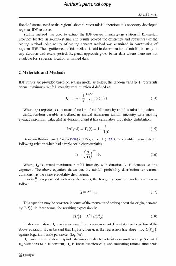
IDF curves are provided based on scaling model as follow, the random variable Id representsannual maximum rainfall intensity with duration d defined as:

Id ¼ max1

d∫

1þd=2

1−d=2x εð Þd εð Þ

" #ð14Þ

Where x(ε) represents continuous function of rainfall intensity and d is rainfall duration.x(ε)Id random variable is defined as annual maximum rainfall intensity with moving

average maximum value x(ε) in duration d and it has cumulative probability distribution:

Pr Id≤ ið Þ ¼ Fd ið Þ ¼ 1−1

T ið Þ ð15Þ

Based on Burlando and Rosso (1996) and Pegram et al. (1999), the variable Id is included infollowing relation when had simple scale characteristics.

Id ¼ d

D

� �−H

:ID ð16Þ

Where, Id is annual maximum rainfall intensity with duration D, H denotes scalingexponent. The above equation shows that the rainfall probability distribution for variousdurations has the same probability distribution.

If ratio Dd is represented with λ (scale factor), the foregoing equation can be rewritten as

follow

Id ¼ λH :Iλd ð17Þ

This equation may be rewritten in terms of the moments of order q about the origin, denoted

by E Iqd� �

; in these terms, the resulting expression is:

E Iqd� � ¼ λHq :E Iqλd

� � ð18ÞIn above equation, Hq is scale exponent for q order moment. If we take the logarithm of the

above equation, it can be said that Hq for given q, is the regression line slope, (log E Iqλd� �

)

against logarithm scale parameter (log (λ)).Hq variations in relation to q indicate simple scale characteristics or multi scaling. So that if

Hq variations to q is constant, Hq is linear function of q and indicating rainfall time scale

Soltani S. et al.


invariance, suggesting scale simplicity. However, variations of Hq to q is not constant, Hq is anon-linear function of q, and representing rainfall multi scaling (Gupta and Waymire 1990).

Figure 1 shows Hq variations to q along with its different conditions. Pegram et al. (1999)showed, in case scale invariance is incorporated in precipitation data, then

μd ¼ λ−Hμλd ð19Þ

σd ¼ λ−Hσλd ð20Þ

Where μd and σd are mean and standard deviation of rainfall intensity in duration drespectively. If rainfall intensity data is characterized with cumulative distribution function F,then rainfall intensity in duration d and return period T can be defined with Chow (1964):

id;T ¼ μd þ KTσd ¼ μd þ σd F−1 1−

1

T

� �ð21Þ

By substituting relations (19) and (20) in above and dividing to d−H, we have:

id;T ¼μλd dλð Þ−H þ σλd dλð Þ−H F−1 1−

1

T

� �d−H

ð22Þ

Where λ−Hμλdand λ−Hσλd are constants coefficients. Comparing (13) and (22) shows that

η = −H,θ = 0,w ¼ μλd dλð Þ−H þ σλd dλð Þ−H F−1 1− 1T

� �As it was stated previously, w is a function of return period T. If dλ is assumed equals with

24, then eq. 22 can be simplified as follow

id;T ¼μ24 24ð Þ−H þ σ24 24ð Þ−H F−1 1−

1

T

� �d−H

ð23Þ

Fig. 1 Simple and multi scaling in term of statistical moments. (a) Moments of different orders q are plotted asfunction of scale in a log-log plot. (b) Linear relation Hq and q process is simple scaling, c) nonlinear relation Hq

and q process is multi scaling



Whereid , T, rainfall intensity with duration d and return period T, is a function of 24 hrainfall characteristics (μ24 σ24).

Thus, using the above equation, which result the theory of rainfall invariance time scales,from daily rainfall data, IDF curves are constructed. In eq. 23, F is Cumulative distributionfunction rainfall intensity. Distributions of extreme rainfall events are usually modeled by oneof the extreme value (EV) distributions, called type I (Gumbel distribution), II, or III, or by thegeneralized extreme value (GEV) distribution.

In this research, based on the dominant distribution of 24 h rainfall intensity of area study,Gumbel distribution was selected. Accordingly, the relation 23 can be rewritten as follows inrelation to the IDF scope of the study area:

id;T ¼μ24 24ð Þ−H−σ24 24ð Þ−HLn −Ln 1−

1

T

� �� d−H

ð24Þ

As for eq. 24, three variables average (μ24), standard deviation of daily rainfall (σ24) andscale exponent (H) can be found. Given these three parameters in one area we can calculaterainfall intensity (IDF curves) in any duration and return period on both point and regionalstatus. Regionalization contains two main objectives. One of the places where their data is notavailable, the analysis is done based on regional data and other places where short record dataare available, the combined use of data at site and regional data from other stations in the area,more complete information for the probability distribution are concluded.

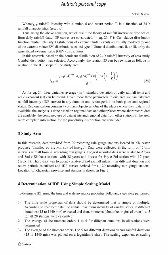
3 Study Area

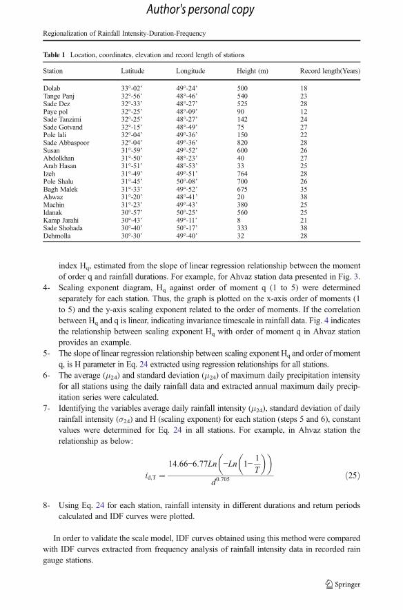
In this research, data provided from 20 recording rain gauge stations located in Khuzestanprovince (installed by the Ministry of Energy). Data were collected in the form of 15-minintervals rainfall from 20 recording rain gauges. Longest recorded data were related to Ahvazand Sad-e Shohada stations with 38 years and lowest for Pay-e Pol station with 12 years(Table 1). These data was frequency analyzed and rainfall intensity in different duration andreturn periods calculated and IDF curves derived for all 20 recording rain gauge stations.Location of Khuzestan province and stations is shown in Fig. 2.

4 Determination of IDF Using Simple Scaling Model

To determine IDF using the time and scale invariance properties, following steps were performed:

1- The time scale properties of data should be determined that is simple or multiple.According to recorded data, the annual maximum intensity of rainfall series in differentdurations (15 to 1440 min) extracted and then, moments (about the origin) of order 1 to 5for all 20 stations were calculated.

2- The average of the moment orders 1 to 5 for different durations in all stations weredetermined.

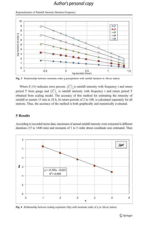
3- The average of the moment orders 1 to 5 for different durations versus rainfall durations(15 to 1440 min) was plotted on a logarithmic chart. The scaling exponent or scaling

Soltani S. et al.


index Hq, estimated from the slope of linear regression relationship between the momentof order q and rainfall durations. For example, for Ahvaz station data presented in Fig. 3.

4- Scaling exponent diagram, Hq against order of moment q (1 to 5) were determinedseparately for each station. Thus, the graph is plotted on the x-axis order of moments (1to 5) and the y-axis scaling exponent related to the order of moments. If the correlationbetween Hq and q is linear, indicating invariance timescale in rainfall data. Fig. 4 indicatesthe relationship between scaling exponent Hq with order of moment q in Ahvaz stationprovides an example.

5- The slope of linear regression relationship between scaling exponent Hq and order of momentq, is H parameter in Eq. 24 extracted using regression relationships for all stations.

6- The average (μ24) and standard deviation (μ24) of maximum daily precipitation intensityfor all stations using the daily rainfall data and extracted annual maximum daily precip-itation series were calculated.

7- Identifying the variables average daily rainfall intensity (μ24), standard deviation of dailyrainfall intensity (σ24) and H (scaling exponent) for each station (steps 5 and 6), constantvalues were determined for Eq. 24 in all stations. For example, in Ahvaz station therelationship as below:

id;T ¼14:66−6:77Ln −Ln 1−

1

T

� �� d0:705

ð25Þ

8- Using Eq. 24 for each station, rainfall intensity in different durations and return periodscalculated and IDF curves were plotted.

In order to validate the scale model, IDF curves obtained using this method were comparedwith IDF curves extracted from frequency analysis of rainfall intensity data in recorded raingauge stations.

Table 1 Location, coordinates, elevation and record length of stations

Station Latitude Longitude Height (m) Record length(Years)

Dolab 33°-02’ 49°-24’ 500 18Tange Panj 32°-56’ 48°-46’ 540 23Sade Dez 32°-33’ 48°-27’ 525 28Paye pol 32°-25’ 48°-09’ 90 12Sade Tanzimi 32°-25’ 48°-27’ 142 24Sade Gotvand 32°-15’ 48°-49’ 75 27Pole lali 32°-04’ 49°-36’ 150 22Sade Abbaspoor 32°-04’ 49°-36’ 820 28Susan 31°-59’ 49°-52’ 600 26Abdolkhan 31°-50’ 48°-23’ 40 27Arab Hasan 31°-51’ 48°-53’ 33 25Izeh 31°-49’ 49°-51’ 764 28Pole Shalu 31°-45’ 50°-08’ 700 26Bagh Malek 31°-33’ 49°-52’ 675 35Ahwaz 31°-20’ 48°-41’ 20 38Machin 31°-23’ 49°-43’ 380 25Idanak 30°-57’ 50°-25’ 560 25Kamp Jarahi 30°-43’ 49°-11’ 8 21Sade Shohada 30°-40’ 50°-17’ 333 38Dehmolla 30°-30’ 49°-40’ 32 28



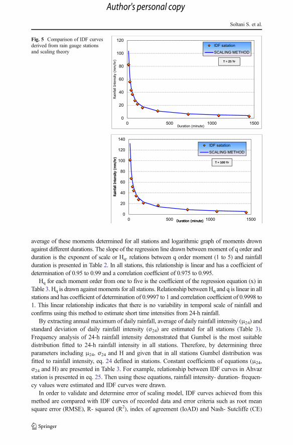
In most previous studies, the graphical method has used to compare the IDF curvesobtained from the scale model and the IDF curves extracted from the rain gauge stations.For example, in Fig. 5, the curves obtained using scale model and data of Ahvaz station arecompared for 25 and 100-year return periods.

In this study, in addition to more accurate graphical method, the accuracy of the methodwas calculated numerically were compared to determine the error of eq. 26:

E Qð Þ ¼ ITt� �

o− ITt� �

e

ITt� �

o

" #*100 ð26Þ

Fig. 2 The location of stations in the Khuzestan province

Soltani S. et al.


Where E (%) indicates error percent, ITt� �

ois rainfall intensity with frequency t and return

period T from gauge and ITt� �

e is rainfall intensity with frequency t and return period T

obtained from scaling model. The accuracy of this method for estimating the intensity ofrainfall to sustain 15 min to 24 h, In return periods of 2 to 100, is calculated separately for allstations. Thus, the accuracy of the method is both graphically and numerically evaluated.

5 Results

According to recorded storm data, maximum of annual rainfall intensity were extracted in differentdurations (15 to 1440 min) and moments of 1 to 5 order about coordinate axis estimated. Then

0

1

2

3

4

5

6

7

8

9

10

-1 -0.5 0 0.5 1 1.5

logmom

ento

forder

q

log dura�on (hour)

q1q2q3q4q5

Fig. 3 Relationship between moments order q precipitation with rainfall duration in Ahvaz station

Fig. 4 Relationship between scaling exponents (Hq) with moments order of q in Ahvaz station



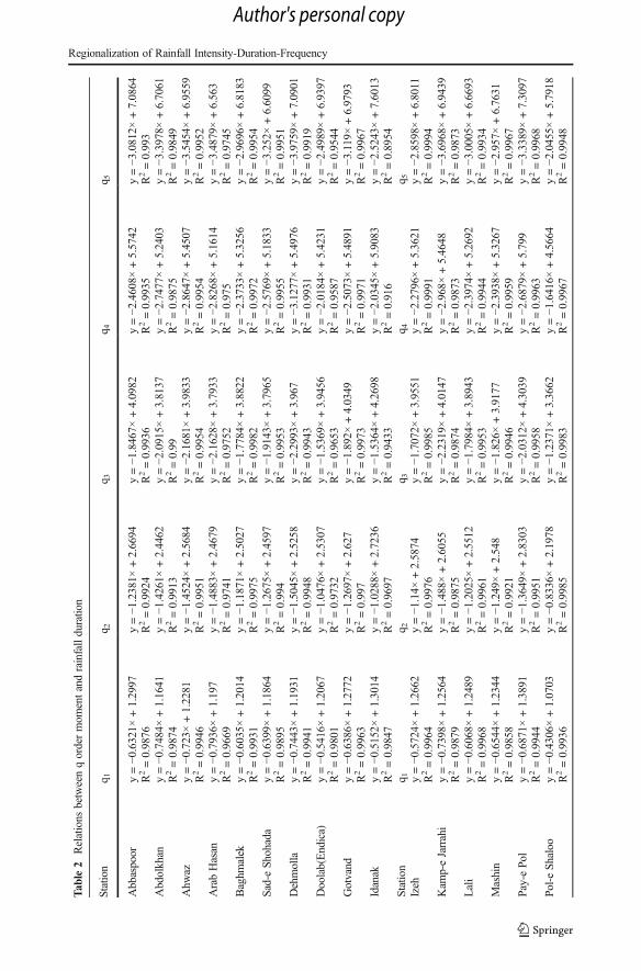
average of these moments determined for all stations and logarithmic graph of moments drownagainst different durations. The slope of the regression line drawn between moment of q order andduration is the exponent of scale or Hq. relations between q order moment (1 to 5) and rainfallduration is presented in Table 2. In all stations, this relationship is linear and has a coefficient ofdetermination of 0.95 to 0.99 and a correlation coefficient of 0.975 to 0.995.

Hq for each moment order from one to five is the coefficient of the regression equation (x) inTable 3. Hq is drawn against moments for all stations. Relationship betweenHq and q is linear in allstations and has coefficient of determination of 0.9997 to 1 and correlation coefficient of 0.9998 to1. This linear relationship indicates that there is no variability in temporal scale of rainfall andconfirms using this method to estimate short time intensities from 24-h rainfall.

By extracting annual maximum of daily rainfall, average of daily rainfall intensity (μ24) andstandard deviation of daily rainfall intensity (σ24) are estimated for all stations (Table 3).Frequency analysis of 24-h rainfall intensity demonstrated that Gumbel is the most suitabledistribution fitted to 24-h rainfall intensity in all stations. Therefore, by determining threeparameters including μ24, σ24 and H and given that in all stations Gumbel distribution wasfitted to rainfall intensity, eq. 24 defined in stations. Constant coefficients of equations (μ24,σ24 and H) are presented in Table 3. For example, relationship between IDF curves in Ahvazstation is presented in eq. 25. Then using these equations, rainfall intensity- duration- frequen-cy values were estimated and IDF curves were drawn.

In order to validate and determine error of scaling model, IDF curves achieved from thismethod are compared with IDF curves of recorded data and error criteria such as root meansquare error (RMSE), R- squared (R2), index of agreement (IoAD) and Nash- Sutcliffe (CE)

0

20

40

60

80

100

120

0 500 1000 1500

IDF satation

SCALING METHOD

T = 25 Yr

0

20

40

60

80

100

120

140

0 500 1000 1500

IDF satation

SCALING METHOD

T = 100 Yr

Fig. 5 Comparison of IDF curvesderived from rain gauge stationsand scaling theory

Soltani S. et al.


Tab

le2

Relations

betweenqordermom

entandrainfallduratio

n

Station

q 1q 2

q 3q 4

q 5

Abbaspoor

y=−0

.6321×

+1.2997

R2=0.9876

y=−1

.2381×

+2.6694

R2=0.9924

y=−1

.8467×

+4.0982

R2=0.9936

y=−2

.4608×

+5.5742

R2=0.9935

y=−3

.0812×

+7.0864

R2=0.993

Abdolkhan

y=−0

.7484×

+1.1641

R2=0.9874

y=−1

.4261×

+2.4462

R2=0.9913

y=−2

.0915×

+3.8137

R2=0.99

y=−2

.7477×

+5.2403

R2=0.9875

y=−3

.3978×

+6.7061

R2=0.9849

Ahw

azy=−0

.723×+1.2281

R2=0.9946

y=−1

.4524×

+2.5684

R2=0.9951

y=−2

.1681×

+3.9833

R2=0.9954

y=−2

.8647×

+5.4507

R2=0.9954

y=−3

.5454×

+6.9559

R2=0.9952

ArabHasan

y=−0

.7936×

+1.197

R2=0.9669

y=−1

.4883×

+2.4679

R2=0.9741

y=−2

.1628×

+3.7933

R2=0.9752

y=−2

.8268×

+5.1614

R2=0.975

y=−3

.4879×

+6.563

R2=0.9745

Baghm

alek

y=−0

.6035×

+1.2014

R2=0.9931

y=−1

.1871×

+2.5027

R2=0.9975

y=−1

.7784×

+3.8822

R2=0.9982

y=−2

.3733×

+5.3256

R2=0.9972

y=−2

.9696×

+6.8183

R2=0.9954

Sad-eSh

ohada

y=−0

.6399×

+1.1864

R2=0.9895

y=−1

.2675×

+2.4597

R2=0.994

y=−1

.9143×

+3.7965

R2=0.9953

y=−2

.5769×

+5.1833

R2=0.9955

y=−3

.252×+6.6099

R2=0.9951

Dehmolla

y=−0

.7443×

+1.1931

R2=0.9941

y=−1

.5045×

+2.5258

R2=0.9948

y=−2

.2993×

+3.967

R2=0.9943

y=−3

.1277×

+5.4976

R2=0.9931

y=−3

.9759×

+7.0901

R2=0.9919

Doolab(Endica)

y=−0

.5416×

+1.2067

R2=0.9801

y=−1

.0476×

+2.5307

R2=0.9732

y=−1

.5369×

+3.9456

R2=0.9653

y=−2

.0184×

+5.4231

R2=0.9587

y=−2

.4989×

+6.9397

R2=0.9544

Gotvand

y=−0

.6386×

+1.2772

R2=0.9963

y=−1

.2697×

+2.627

R2=0.997

y=−1

.892×+4.0349

R2=0.9973

y=−2

.5073×

+5.4891

R2=0.9971

y=−3

.119×+6.9793

R2=0.9967

Idanak

y=−0

.5152×

+1.3014

R2=0.9847

y=−1

.0288×

+2.7236

R2=0.9697

y=−1

.5364×

+4.2698

R2=0.9433

y=−2

.0345×

+5.9083

R2=0.916

y=−2

.5243×

+7.6013

R2=0.8954

Station

q 1q 2

q 3q 4

q 5Izeh

y=−0

.5724×

+1.2662

R2=0.9964

y=−1

.14×

+2.5874

R2=0.9976

y=−1

.7072×

+3.9551

R2=0.9985

y=−2

.2796×

+5.3621

R2=0.9991

y=−2

.8598×

+6.8011

R2=0.9994

Kam

p-eJarrahi

y=−0

.7398×

+1.2564

R2=0.9879

y=−1

.488×+2.6055

R2=0.9875

y=−2

.2319×

+4.0147

R2=0.9874

y=−2

.968×+5.4648

R2=0.9873

y=−3

.6968×

+6.9439

R2=0.9873

Lali

y=−0

.6068×

+1.2489

R2=0.9968

y=−1

.2025×

+2.5512

R2=0.9961

y=−1

.7984×

+3.8943

R2=0.9953

y=−2

.3974×

+5.2692

R2=0.9944

y=−3

.0005×

+6.6693

R2=0.9934

Mashin

y=−0

.6544×

+1.2344

R2=0.9858

y=−1

.249×+2.548

R2=0.9921

y=−1

.826×+3.9177

R2=0.9946

y=−2

.3938×

+5.3267

R2=0.9959

y=−2

.957×+6.7631

R2=0.9967

Pay-ePo

ly=−0

.6871×

+1.3891

R2=0.9944

y=−1

.3649×

+2.8303

R2=0.9951

y=−2

.0312×

+4.3039

R2=0.9958

y=−2

.6879×

+5.799

R2=0.9963

y=−3

.3389×

+7.3097

R2=0.9968

Pol-eSh

aloo

y=−0

.4306×

+1.0703

R2=0.9936

y=−0

.8336×

+2.1978

R2=0.9985

y=−1

.2371×

+3.3662

R2=0.9983

y=−1

.6416×

+4.5664

R2=0.9967

y=−2

.0455×

+5.7918

R2=0.9948



Tab

le2

(contin

ued)

Station

q 1q 2

q 3q 4

q 5

Sad-eDez

y=−0

.6095×

+1.2865

R2=0.9948

y=−1

.2492×

+2.6853

R2=0.995

y=−1

.914×+4.1773

R2=0.9937

y=−2

.5916×

+5.736

R2=0.9914

y=−3

.2723×

+7.3377

R2=0.9885

Sad-eTanzim

iy=−0

.7906×

+1.2746

R2=0.9537

y=−1

.4967×

+2.6648

R2=0.9668

y=−2

.2245×

+4.1688

R2=0.9645

y=−2

.9746×

+5.7657

R2=0.958

y=−3

.738×+7.4205

R2=0.9516

Soosan

y=−0

.5119×

+1.2131

R2=0.999

y=−1

.0176×

+2.4982

R2=0.9992

y=−1

.5268×

+3.8452

R2=0.9992

y=−2

.0404×

+5.2418

R2=0.999

y=−2

.557×+6.6748

R2=0.9982

Tang-e

Panj

y=−0

.5024×

+1.4295

R2=0.9987

y=−1

.0167×

+2.939

R2=0.9985

y=−1

.5492×

+4.5121

R2=0.9975

y=−2

.097×+6.1351

R2=0.9959

y=−2

.6563×

+7.7961

R2=0.9938

Soltani S. et al.


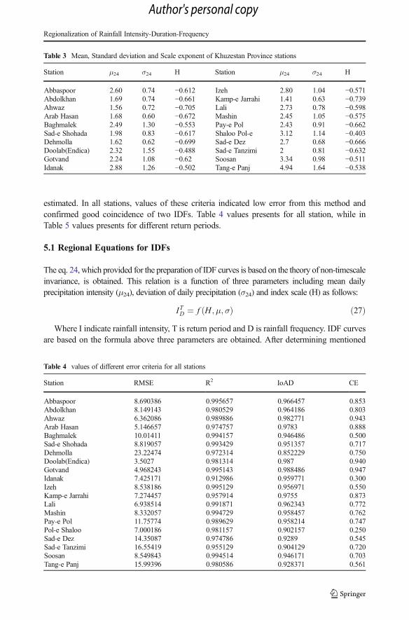
estimated. In all stations, values of these criteria indicated low error from this method andconfirmed good coincidence of two IDFs. Table 4 values presents for all station, while inTable 5 values presents for different return periods.

5.1 Regional Equations for IDFs

The eq. 24, which provided for the preparation of IDF curves is based on the theory of non-timescaleinvariance, is obtained. This relation is a function of three parameters including mean dailyprecipitation intensity (μ24), deviation of daily precipitation (σ24) and index scale (H) as follows:

ITD ¼ f H ;μ;σð Þ ð27ÞWhere I indicate rainfall intensity, T is return period and D is rainfall frequency. IDF curves

are based on the formula above three parameters are obtained. After determining mentioned

Table 3 Mean, Standard deviation and Scale exponent of Khuzestan Province stations

Station μ24 σ24 H Station μ24 σ24 H

Abbaspoor 2.60 0.74 −0.612 Izeh 2.80 1.04 −0.571Abdolkhan 1.69 0.74 −0.661 Kamp-e Jarrahi 1.41 0.63 −0.739Ahwaz 1.56 0.72 −0.705 Lali 2.73 0.78 −0.598Arab Hasan 1.68 0.60 −0.672 Mashin 2.45 1.05 −0.575Baghmalek 2.49 1.30 −0.553 Pay-e Pol 2.43 0.91 −0.662Sad-e Shohada 1.98 0.83 −0.617 Shaloo Pol-e 3.12 1.14 −0.403Dehmolla 1.62 0.62 −0.699 Sad-e Dez 2.7 0.68 −0.666Doolab(Endica) 2.32 1.55 −0.488 Sad-e Tanzimi 2 0.81 −0.632Gotvand 2.24 1.08 −0.62 Soosan 3.34 0.98 −0.511Idanak 2.88 1.26 −0.502 Tang-e Panj 4.94 1.64 −0.538

Table 4 values of different error criteria for all stations

Station RMSE R2 IoAD CE

Abbaspoor 8.690386 0.995657 0.966457 0.853Abdolkhan 8.149143 0.980529 0.964186 0.803Ahwaz 6.362086 0.989886 0.982771 0.943Arab Hasan 5.146657 0.974757 0.9783 0.888Baghmalek 10.01411 0.994157 0.946486 0.500Sad-e Shohada 8.819057 0.993429 0.951357 0.717Dehmolla 23.22474 0.972314 0.852229 0.750Doolab(Endica) 3.5027 0.981314 0.987 0.940Gotvand 4.968243 0.995143 0.988486 0.947Idanak 7.425171 0.912986 0.959771 0.300Izeh 8.538186 0.995129 0.956971 0.550Kamp-e Jarrahi 7.274457 0.957914 0.9755 0.873Lali 6.938514 0.991871 0.962343 0.772Mashin 8.332057 0.994729 0.958457 0.762Pay-e Pol 11.75774 0.989629 0.958214 0.747Pol-e Shaloo 7.000186 0.981157 0.902157 0.250Sad-e Dez 14.35087 0.974786 0.9289 0.545Sad-e Tanzimi 16.55419 0.955129 0.904129 0.720Soosan 8.549843 0.994514 0.946171 0.703Tang-e Panj 15.99396 0.980586 0.928371 0.561



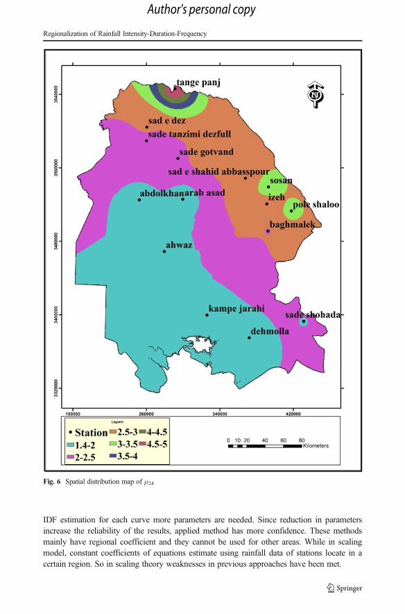
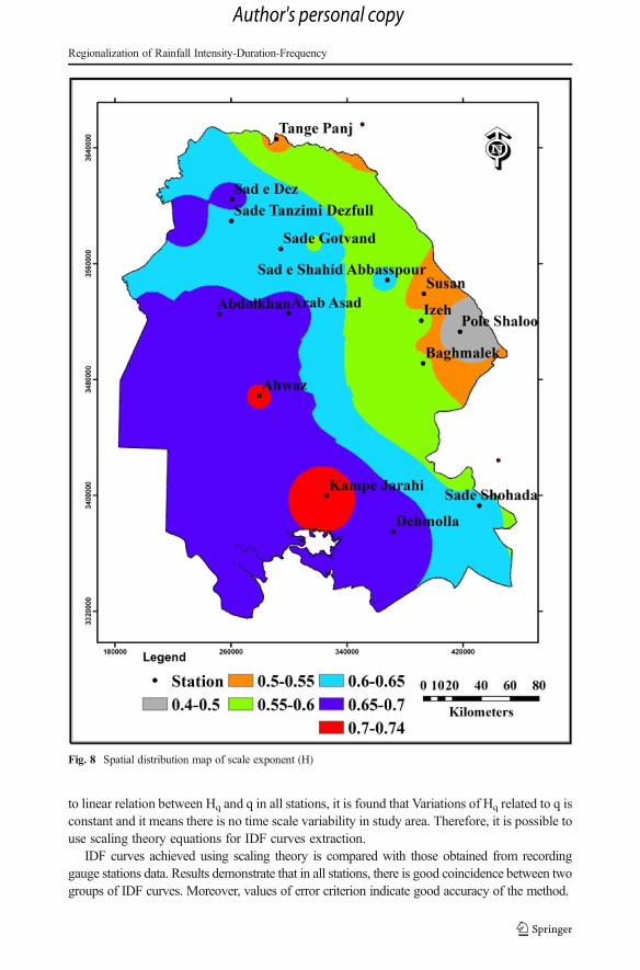
parameters (μ24,σ24 and H), three spatial distribution maps of these parameters are preparedusing interpolation techniques in Arc- GIS the study area. Thus, by using the obtained valuesfor each parameter in the rain gauge stations located in Khuzestan, spatial distribution maps ofthese three parameters were determined using the interpolation in Arc- GIS. Figures 6, 7, 8represent the distributed maps forμ24,σ24 and H, respectively. Based on these maps, valuesofμ24,σ24 and H estimate for any point or area with no recorded rainfall data and then, by usingthese parameters, constant coefficients of eq. 24 including μ24(24)

−H and σ24(24)−H are

determined. By determining the amount of these two coefficients, for each point or area,IDF curves relationships obtain with only two unknown variables (d and T). So IDFs can bedefined in given point or region only by entering different return periods (in terms of year) andduration (in term of hour) in mentioned equation.

If μ24, σ24 and H extract for a specific point, IDF achieved from equation is a point. But ifthese variables use as weighted average of a basin or a region, IDF curves derived from themare regional IDFs that are of great importance and application in hydrological studies.

6 Discussion and Conclusion

In present study, the efficiency and accuracy of the scaling theory in IDF curves extraction areevaluated by using daily rainfall and comparing estimated IDFs based on scaling model andrecorded data in the southwestern Iran as the first study of its type. The Khuzestan provinceincluded both mountainous and plain regions that are compared for their scale invariance IDFproperties whichwere compared in this study as one of its new findings. In addition, the parametersof scaling characteristics are shown in a spatial view which is also one of new representation to theliterature. As the Khuzestan province is a flood-prone area with heavy rainfall, this study alsobrings deeper insights for flood analysis in future across the study region.

From technical points of view, we can conclude that most of the empirical equations usingto estimate IDF curves have regional coefficients which determined for specific climaticconditions and cannot be used for other areas. Moreover, these methods present IDF curvesjust for a specific point and are not capable to determine regional IDF curves that are ofparticular importance in hydrological studies. On the other hand, most of previous methods inaddition to complexity, number of parameters, and length of relationship, short term rainfall(e.g. 1- h 10- year rainfall) is used which is only able to be estimated in recording rain gaugestations and in the absence of this information, it is impossible to identify IDF curves.

The advantage of this approach over previous methods is that experimental methods haveregional coefficients which have been determined for specific climatic conditions and cannotbe used for other areas. While, in scaling invariance method constant coefficients of equationsis derived using rainfall data from stations located in a certain region. Moreover, in scalingmethod IDF curves are drawn just by using three parameters, while in common methods for

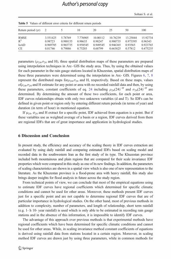
Table 5 Values of different error criteria for different return periods

Return period (yr) 2 5 10 20 25 50 100

RMSE 3.551425 5.78769 7.776905 10.00112 10.76239 13.25044 15.92734R2 0.98723 0.988155 0.98635 0.98247 0.980735 0.973595 0.96343IoAD 0.969785 0.965735 0.958545 0.949545 0.946365 0.93565 0.923765CE 0.81746 0.79886 0.75203 0.68799 0.663825 0.57812 0.475235

Soltani S. et al.


IDF estimation for each curve more parameters are needed. Since reduction in parametersincrease the reliability of the results, applied method has more confidence. These methodsmainly have regional coefficient and they cannot be used for other areas. While in scalingmodel, constant coefficients of equations estimate using rainfall data of stations locate in acertain region. So in scaling theory weaknesses in previous approaches have been met.

Fig. 6 Spatial distribution map of μ24



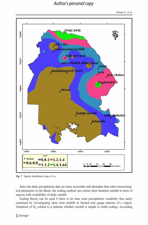
Since the daily precipitation data are more accessible and abundant than other meteorolog-ical parameters in the Basin, the scaling method can extract short duration rainfall in most ofregions with availability of daily rainfall.

Scaling theory can be used if there is no time scale precipitation variability that easilyexamined by investigating short term rainfall in limited rain gauge stations of a region.Variations of Hq related to q indicate whether rainfall is simple or multi scaling. According

Fig. 7 Spatial distribution map of σ24

Soltani S. et al.


to linear relation between Hq and q in all stations, it is found that Variations of Hq related to q isconstant and it means there is no time scale variability in study area. Therefore, it is possible touse scaling theory equations for IDF curves extraction.

IDF curves achieved using scaling theory is compared with those obtained from recordinggauge stations data. Results demonstrate that in all stations, there is good coincidence between twogroups of IDF curves. Moreover, values of error criterion indicate good accuracy of the method.

Fig. 8 Spatial distribution map of scale exponent (H)



Mean absolute error for presented equations mainly is under 25% and only in fewcases error is higher than 25%. Error higher than 25% mainly is seen in durations greaterthan 6 h (e.g. 12, 18 and 24 h durations). So it can be said that the estimated values ofrainfall intensity in different durations and return periods present better results for rainfallwith duration up to 6 h. Comparison of error criteria related to two IDF curves groupsshow that for rainfalls with duration up to 6 h, minimum of mean error differ from 8% inAhvaz station to 13.7% in Izeh station. Likewise, maximum of mean error is differentfrom 9% in Dehmolla to 35.5% in Baghmalek station. Moreover, results indicate thatamong 20 recording rain gauge stations, in 13 stations average of estimated error indifferent durations (15 min to 6 h) is lower than 20%. These stations are mostly locatedin northern and central parts of Khuzestan province. In other words, scaling method ismore accurate in mentioned parts and can be used with high sureness in these areas.While, error rate of scaling model is high in Pol-e shalu, Idanak and Izeh and increase inhigher return periods. It may relate to microclimate conditions of these stations or rainfallcharacteristics. However, more detailed studies are needed to determine the reasons forerror rates. It is also worth noting that error value is consistent with the range reported inthe literature. For example, Pagliara and Viti (1993) suggested the range of ±20% forerrors in Italy. Kothyari and Garde (1992) estimated the error rate of ±30% for India.Likewise, Ghahraman et al. (2010) provided a maximum error of about 19% forKhorasan Province in Iran.

Error in the mountainous area is more than flat ones. Data availability for longer period,lead to better coincidence and more accurate results (e.g. Ahvaz and Abbaspoor stations). Errorrate increases by raising return periods, since increased uncertainty in interpolation. Rainfallintensity values obtained from the scaling model for different durations and return periods arein 95% confidence level result from storm frequency analysis of rain gauge stations. Therefore,estimated error for scaling model seems reasonable.

One of the most important capabilities of scaling model is IDF curves extraction for regionswith no data. To determine IDF relations for these regions or define regional IDFs, equationscan be provided with the help of three parameters including average of daily rainfall intensity(μ24), standard deviation of daily rainfall (σ24) and scale exponent (H) in any point and so justby entering intended duration and return period, corresponding rainfall intensity is achieved.

By using regional values of parameters μ24, σ24 and H and presented equation for eachstation, IDF curves are determined for any point or area. Previous methods provide IDF curvesas a point and they are not able to define regional curves which are of great importance inhydrological studies. While, in scaling method IDF curves can be provided in a regional orpoint way based on the purpose of study.

References

Bell FC (1969) Generalized rainfall-duration-frequency relationships. J Hydraul Div 95(1):311–327Bernard MM (1932) Formulas for rainfall intensities of long duration. Trans Am Soc Civ Eng 96(1):592–606Blanchet J, Ceresetti D, Molinié G, Creutin J-D (2016) A regional GEV scale-invariant framework for intensity–

duration–frequency analysis J. Hydrol 540:82–95. doi:10.1016/j.jhydrol.2016.06.007Burlando P, Rosso R (1996) Scaling and multi scaling models of depth-duration-frequency curves for storm

precipitation. J Hydrol 187(1):45–64Chen CL (1983) Rainfall intensity-duration-frequency formulas. J Hydraul Eng 109(12):1603–1621Chow VT (1964) Handbook of applied hydrology. McGraw-Hill, New York

Soltani S. et al.


http://dx.doi.org/10.1016/j.jhydrol.2016.06.007

Diaconis P, Efron B (1983) Computer intensive methods in statistics. Sci Am 248(5):116–130Elsebaie IH (2012) Developing rainfall intensity–duration–frequency relationship for two regions in Saudi

Arabia. Journal of King Saud University – Engineering Sciences 24(2):131–140. doi:10.1016/j.jksues.2011.06.001

Ghahraman B (1995) A general dimensionless rainfall depth- duration- frequency relationship. AgriculturalResearch Journal 14:217–235

Ghahraman B. (1998) A comprehensive study of June 6, 1992 storm in Mashhad. J.WSS. 2003; 7 (2):29-41Ghahraman B, Abkhezr HR (2004) Improvement in intensity-duration-frequency relationships of rainfall in Iran.

JWSS 8(2):1–14Ghahraman B, Shamkoian H, Davari K (2010) Derivation of the regional rainfall depth-duration-frequency

equations using linear moment theories (case study: Khorasan provinces). Iranian Journal of irrigation anddrainage 4(1):132–142

Ghahramn B., Sepaskhah A.R. (1990) Intensity-duration-frequency estimation in Iran using 1-hour, 10- yearrainfall, third international congress of civil engineering, Iran, pp. 35-55.

Ghanmi H, Bargaoui Z, Mallet C (2016) Estimation of intensity-duration-frequency relationships according tothe property of scale invariance and regionalization analysis in a Mediterranean coastal area. J. Hydrol.541(a):38–49. doi:10.1016/j.jhydrol.2016.07.002

Gupta VK, Waymire E (1990) Multi scaling properties of spatial and river flow distributions. J Geophys Res95(D3):l999–2009

Kothyari UC, Garde RJ (1992) Rainfall intensity-duration-frequency formula for India. J Hydraul Eng ASCE118:323–336. doi:10.1061/(ASCE)0733-9429(1992)118:2(323)

Koutsoyiannis D, Kozonis D, Manetas A (1998) A mathematical framework for studying rainfall intensity-duration-frequency relationships. J Hydrol 206(1):118–135

Kumar BA, Khosa R, Maheswaran R (2016) Developing intensity duration frequency curves based on scalingtheory using linear probability weighted moments: a case study from India. J Hydrol 542:850–859.doi:10.1016/j.jhydrol.2016.09.056

Mirhosseini G, Srivastava P, Stefanova L (2013) The impact of climate change on rainfall intensity–duration–frequency (IDF) curves in Alabama. Reg Environ Chang 13(S1):25–33

Nguyen VTV, Nguyen TD, Ashkar F (2002) Regional frequency analysis of extreme rainfalls. Water Sci Technol45(2):75–81

Nhat LM, Tachikawa Y, Takaka K (2006) Establishment of IDF relationships for monsoon areas, annual of Disas.Prev. Rrev. Inst. Kyoto University, No 49(B):93–103

Noori Gheidari MH (2009) Derivation of rainfall intensity – duration – frequency relationships for short-durationrainfall from daily data, fifth national conference on watershed management science and engineering.Gorgan university of agricultural sciences and natural resources, Iran

Pagliara S, Viti C (1993) Discussion of Brainfall intensity-duration-frequency formula for India^ by Umesh C.Kothyari and Ramachandra J. Garde (February, 1992, Vol. 118, no. 2). J Hydraul Eng 119(8):962–966

Pegram G, Menabde M, Seed A (1999) A simple scaling model for extreme rainfall. Water Resour Res 35(1):335–339

Rasel M, Hossain SM (2015) Development of rainfall intensity duration frequency (R-IDF) equations and curvesfor seven divisions in Bangladesh. International Journal of Scientific & Engineering Research 6(5):96–101

Sherman CW (1931) Frequency and intensity of excessive rainfalls at Boston, Massachusetts. Trans Am Soc CivEng 95(1):951–960

Sivapalan M, Blöschl G (1998) Transformation of point rainfall to areal rainfall: intensity- duration-frequencycurves. J Hydrol 204(1):150–167

Vaziri F (1984) Analysis of storms and determination of the intensity curves for different regions of Iran.Academic Jihad, unit of Tehran, Iran

Vaziri F (1992) Determination of regional relations for short-term rainfall in Iran. Academic Jihad, unit of Khajenasir, Iran

Yu PS, Yang TC, Lin CS (2004) Regional rainfall intensity formulas based on scaling property of rainfall. JHydro 295(1):108–123

Zope P, Eldho TI, Jothiprakash V (2016) Development of rainfall intensity duration frequency curves forMumbai city, India. Journal of water resource and protection 8:756–765. doi:10.4236/jwarp.2016.87061



http://dx.doi.org/10.1016/j.jksues.2011.06.001

http://dx.doi.org/10.1016/j.jksues.2011.06.001


http://dx.doi.org/10.1061/(ASCE)0733-9429(1992)118:2(323)


http://dx.doi.org/10.4236/jwarp.2016.87061

Dr.Reza Modarres | Assisstant Professor, Faculty of ...

Documents

Transcript of Dr.Reza Modarres | Assisstant Professor, Faculty of ...