First Draft, December 2003 This Draft, October 28th 2007 Preliminary, not for quotation

Characteristics of Observed Demand and Supply Schedules for

Individual Stocks

Jung-Wook Kim, a Jason Lee, b and Randall Morck c Abstract

Using complete limit order books from the Korea Stock Exchange for a three year period including the 1998 Asian financial crisis, we observe (not estimate) demand and supply curves for individual stocks. Both curves have demonstrably finite elasticities, which fall markedly with the crisis and remain depressed long after other economic and financial variables revert to pre-crisis norms. Although they share this common long-term trend, the magnitudes of individual stocks’ supply and demand elasticities are negatively correlated at higher frequencies. That is, when a stocks exhibits an unusually elastic demand curve, it tends simultaneously to exhibit an unusually inelastic supply curve, and vice versa. This high frequency negative correlation also swells with the crisis. These findings have potential implications for modeling how information flows into and through stock markets, how investors react to information flows, and how new information is capitalized into stock prices. We advance speculative hypotheses, and invite further work – including theory papers – to explain these findings and their implications. JEL classification: G10; G14

Keywords: Supply and Demand; Elasticity; Stocks; Information Cost; Information Set Heterogeneity; Financial Crisis

a. Jung-Wook Kim is Assistant Professor of Finance at the University of Alberta, Edmonton Alberta, Canada T6G 2R6. Phone (780) 492-7987, fax (780) 492-3325, e-mail jungwook.kim@ualberta.ca.

b. Jason Lee is Associate Professor of Accounting at the University of Alberta, Edmonton Alberta, Canada T6G 2R6. Phone (780) 492-4839, fax (780) 492-3325, e-mail jasonlee@ualberta.ca.

c. Randall K. Morck is Stephen A. Jarislowsky Distinguished Professor of Finance and University Professor at the University of Alberta, Edmonton Alberta, Canada T6G 2R6. Phone (780) 492-5683, fax (780) 492-3325, e-mail randall.morck@ualberta.ca. He is also a Research Associate of the National Bureau of Economic Research, and this research was undertaken partly when he was Visiting Professor of Economics at Harvard University.

We thank Hyeon Kee Bae, Utpal Bhattacharya, Wonseok Choi, Mark Huson, Aditya Kaul, Alok Kumar, Ki Bong Lee, Kyung-Mook Lim, Vikas Mehrotra, Jeff Pontiff, Barry Scholnick, Andrei Shleifer, Jeremy Stein, students in Andrei Shleifer’s behavioral finance seminar course at Harvard University, and seminar participants at the University of Alberta for helpful comments. We gratefully acknowledge financial support from University Alberta SAS fellowship and the Social Sciences and Humanities Research Council.

1

1. Introduction

A complete dataset of all orders, each flagged as a buy or sell, for all Korean listed stocks

from Dec. 1996 to Dec. 2000 lets us observe the whole demand and supply curves of limit

orders for each individual listed stock at any instant in time. We do this twice each day –

once at the beginning of trading and again half an hour before the market closes. Since the

market opens with a call auction session but then switches to continuous trading, this lets us

explore demand and supply under the two microstructure alternatives. Since our sample

period includes 1998, we also observe demand and supply curves of common stocks before,

during, and after the Asian financial crisis.

Because we observe entire demand and supply curves, we can gauge the elasticity of

each curve separately and directly, rather than jointly and by inference from prices and

quantities traded. This lets us sidestep entirely the standard simultaneity problems associated

with elasticity estimation. Moreover, it also lets us compare the two elasticities and

investigate the relationship between them. To the best of our knowledge, this is the first study

to investigate these issues.

First, the absolute values of both demand and supply elasticities exhibit a common

long run trend. Before the Asian crisis, both average around forty. That is, a one percent price

change commands a forty percent change in quantity demanded or supplied. Both absolute

values drop to roughly twenty after the crisis. Unlike many other economic and financial

indicators, which fluctuate dramatically around the crisis before reverting to their pre-crisis

levels, individual stocks’ elasticities remain at these new average levels – apparently

permanently. The direction of this shift is counterintuitive, for transparency is widely thought

enhanced and transactions costs reduced (by the advent of on-line trading) in the post-crisis

period.

2

Second, superimposed on this common long run trend, the absolute values of the two

elasticities exhibit a negative correlation at higher frequencies. That is, stocks that develop

unusually elastic demand curves tend simultaneously to develop unusually inelastic supply

curves and vice versa. This correlation is more negative in 2:30 PM elasticities than in

opening auction elasticities. The negative correlation in opening elasticities swells after the

crisis; as does that in 2:30 PM elasticities, though mainly for larger firms.

We also find supply curves to be more elastic than demand curves on average. This

differs from Kalay et al. (2004), who find higher local elasticities (estimated using limit

orders near market prices) for demand curves in Tel Aviv data. The difference suggests that

circumstances specific to sample periods or market structures may matter. We corroborate

Kalay et al. (2004) in finding higher mean elasticities at 2:30 PM than in opening auctions,

but our median elasticities do not exhibit this pattern.

Overall, our results support theories of information capitalization derived from

Harrison and Kreps (1978), Grossman and Stiglitz (1980), and others; in which market prices

arise from the intersection of finitely elastic demand and supply curves for each stock. Asset

pricing models that postulate infinitely elastic demand and supply for individual stocks may

be useful approximations under some circumstances, but these require clarification.

The remainder of the paper is organized as follows. Section 2 overviews relevant

work; while section 3 discusses the data and elasticity measurement procedure. Section 4

describes our findings. Section 5 investigates possible explanations, and section 6 concludes.

2. Relation to Previous Studies The wheel horses of asset pricing (Markowitz, 1952; Tobin, 1958; Sharpe, 1964; Lintner,

1965) postulate that individual stocks have infinitely many perfect substitutes in other stocks

or portfolios, and so have horizontal demand and supply curves. In contrast, asset prices

3

given costly information or incomplete arbitrage are determined by finitely elastic supply and

demand curves for individual stocks, as in Grossman and Stiglitz (1980). Basic models of

this ilk posit demand and supply elasticities as functions of investor risk aversion and

certainty about fundamental values. All else equal, greater risk aversion and worse

uncertainty imply more heterogeneous fundamental value estimates, and hence less elastic

demand and supply curves. Subsequent elaborations include Blough (1988), who models

heterogeneous information; Hindy (1989), who has different investors using different models

to process common information; De Long et al. (1990), who model noise traders formally;

Kandel and Peason (1992), who assign different priors to different investors; and Harris and

Raviv (1993) who model differences of opinion more generally.

The virtues of the wheel horses are elegance and simplicity; those of the Grossman

and Stiglitz framework are explicit recognition of information costs and more realistic

treatment of the economics of the investment industry (Shleifer and Vishny, 1997). The latter

advantages are nontrivial, for Varian (1985, 1989), Shleifer and Vishny (1997), Shleifer

(2000), Shiller (2002), and many others argue that information per se is costly. Shleifer and

Vishny (1997) go further, arguing that unavoidable information asymmetries and agency

problems in firms in the financial sector create economically significant transactions costs to

informed trading, even on free private information. These considerations allow different

investors to persist in holding different beliefs about individual stocks’ values, directly

implying finitely elastic demand and supply curves.

A growing literature supports persistent information heterogeneity across investors,

and thus the second class of models. Varian (1985, 1989) argues that normal trading volume

is inconsistent with homogenous stock valuations, and implies heterogeneous investor beliefs.

Barber and Odean (2000), Shleifer (2000), Grinblatt and Han (2005) attribute this

heterogeneity to behavioral biases. But Varian (1985, 1989), Kandel and Pearson (1995),

4

Fama and French (2007) all permit difference in opinion among rational investors. In either

case, different investors perceive one stock as having different fundamental values. This

directly implies finitely elastic demand and supply curves for that stock.

Scholes (1972) thus rightly stresses the importance of gauging these elasticities.

Unable to observe these curves directly, he examines stock price drops upon secondary

offerings announcements and concludes that these reflect negative information conveyed by

firms’ decisions to issue shares, not finite elasticities. Mikkelson and Partch (1985) revisit

the issue, concluding supply and demand elasticities for individual stocks to be very large.

But others dissent. Shleifer (1986), Harris and Gruel (1986), Jain (1987), Dhillon and

Johnson (1991), Beamish and Whaley (1996), Lynch and Mendenhall (1997), Blouinet

(2000), Liu (2000), and others report share price increases when stocks are added to widely

followed indexes. Shleifer attributes this to finitely elastic demand curves shifted right by

index funds share purchases. But Jain (1987), Dhillon and Johnson (1991), and others argue

that inclusion in an index conveys positive information about a stock; while Harris and Gruel

(1986), Blouinet (2000), and others argue for a temporary price pressure effect, whereby

index fund purchases elevate prices only until arbitrageurs’ trades reverse the effect. Kaul et

al. (2000) examine the reweighting of a widely tracked Canadian index, and find permanent

price elevations for stocks whose weights rise and permanent price decreases for those whose

weights fall. Since no stocks are added to the index and the reweighting is announced

months in advance, an information effect is excluded. Since the effects do not reverse, price

pressure is also untenable. In contrast, Greenwood (2003) examines a similar reweighting in

Japan, and finds a complete reversal.

Thus, despite much work, generalizations about elasticities of supply and demand for

individual common stocks remain elusive.

5

Simultaneity problems persist wherever elasticities are inferred indirectly from the

price impacts of certain events. If factors that affect demand also affect supply, identification

problems arise and biases ensue. In goods markets, these can be mitigated if appropriate

strong instruments are available to distinguish e.g. technology from preference shocks. But

the stock market is a pure exchange market, whose traders are all plausibly affected by

similar factors simultaneously.

This obliges alternative approaches. Thus, Bagwell (1992) examine stock

repurchases; while Kandel et al. (1999) and Liaw et al. (2000) study IPOs auctions. All find

finite elasticities, but also all pertain to special corporate events, not normal trading days.

Kalay et al. (2004) measure supply and demand elasticities for Tel Aviv stocks from

limit orders adjacent to market prices. They report unambiguously finite elasticities, but

caution that their estimates depend critically on their assumptions. Specifically, they estimate

elasticities as percentage change in quantity divided by percentage change in price and take

the former to be the quantity offered or sought divided by the ‘total quantity of shares’. If

this is ‘total shares outstanding’, the elasticities are small, but if ‘total daily volume’ is used

instead they are much larger. Other alternatives they do not explore might include ‘total

public float’ or a ‘smoothed trading volume’. To sidestep these ambiguities, we estimate

elasticity as the difference in log quantity offered or sought divided by the difference in log

prices. This lets the data choose a denominator implicit in the slope of the curve being

estimated.

Another factor that might distort estimated elasticities is strategic liquidity provision.1

Hollifield et al. (2004, 2006) expand the framework of Grossman and Stiglitz (1980) to

derive liquidity provider’s optimal limit order strategy from her fundamental value estimate

and on a trade-off between execution probability and ‘picking off’ risk – the risk of trading

1 See Obzhaeva and Wang (2005), Hollifield et al. (2004, 2006), and references therein on optimal order submission strategy in a limit order market.

6

against better informed investors. Limit orders placed nearer the market price have a higher

execution probability, but entail worse ‘picking off’ risk. Thus, the limit order book reflects

inseparably confounded strategic liquidity provision and information heterogeneity (p. 2760):

“Traders with high private values submit buy orders with high execution probabilities.

Traders with low private values submit sell orders with high execution probabilities. Traders

with intermediate private values either submit no orders, or submit buy or sell orders with

low execution probabilities.” That is, heterogeneous valuations across investors induce a

distribution of limit orders across prices, and hence finitely elastic demand and supply curves,

for individual stocks.

Hollifield et al. (2004, 2006) focus on expected trading revenues because they analyze

risk neutral investors, and thus provide a state-of-the-art platform on which to build more

complete descriptions of limit order distributions that account for different risk aversion,

uncertainty as to fundamental values, signal extraction processes, or learning patterns. For

example, extending their intuition to a world of risk-averse investors should presumably

magnify the broadening effect ‘picking off’ risk on limit order distributions. Elasticities

would then become smaller as risk aversion or uncertainty about fundamentals rises. Another

useful theoretical extension would encompass investors’ reaction functions to each others’

trades. As trades execute at changing prices, limit order providers learn each others’ opinions

and use this information to update their estimates of fundamental value and hence their limit

orders.

The last point seems especially important given Roll (1988), who shows that stock

price fluctuations usually do not correspond to public information events. From this, he infers

that stock price changes are typically caused by investors seeking to gain from private

information they acquire. This suggests that traders on one side of the limit order book may

often be at an information advantage to those on the other side. For example, if a subset of

7

investors learns a stock is underpriced, they should enter large buy orders at or just above the

market, flattening the demand curve. Seeing these execute, uninformed sell-side investors

would presumably withdraw limit order depth near the market, steepening the supply curve.

Consistent with the intuition underlying these conjectures, Kavajecz (1999) finds

specialists and limit order traders in the US reducing depths around information events; and

Goldstein and Kavajec (2004) report limit order traders remaining inactive or even

withdrawing when the plummeting Dow Jones Industrial Average triggered circuit breakers

that halted all trading on October 27, 1997.

3. Measuring Elasticities

This section describes how we measure elasticities of demand and supply of individual stocks.

It first describes the trading system of the KSE and the raw trade and quote data it generates,

then how we construct demand and supply schedules for each stock twice a day, and finally

how we summarize the shape of those curves into elasticities.

3.1 Market Microstructure

The KSE is an order driven market, in that it has no designated market makers or specialists.

Any investor is free to make a market in any stock, however this entails certain costs. All

investors, including brokers, pay a 0.3% stamp tax on executed sales. Online trading started

in 1997 with fees of 0.5%, matching standard brokerage fees at the time. But online fees fell

sharply after June 1998 as competition began in earnest. Tick sizes depend on a stock’s price

range – a ₩5,000 stock is priced in ₩5 increments, while a ₩50,000 stock is priced in ₩50

ticks.2 Bid-ask spreads are thus not entirely endogenous.

The investor base also changes with time. Before May 1998, foreign ownership was 2 The Korean currency, the won, trades at approximately ₩1,000 per American dollar. For details on tick sizes, see www.kse.or.kr/webeng.

8

restricted, presumably limiting foreigners ability to take large positions in the stock of firms

with large stable forign blockholdings. After May 1998, all such restrictions disappeared.

Trading begins at 09:00 with a call market – an auction in which accumulated bids

and offers, taken as simultaneous, are matched to generate one opening price for each stock.

In our data, 19.10 percent of buy orders and 21.14 percent of sell orders are submitted to

opening sessions.

Subsequent prices, until 10 minutes before the closing time at 15:00 are set in

continuous trading. 3 In the last 10 minutes, another auction market session determines prices.

Orders not fully filled in the opening auction pass into continuous trading unless cancelled or

revised. An automatic trading system records all outstanding limit orders and automatically

crosses new market and limit orders with these, or with opposite market orders.4 The

computerized order-routing system prioritizes by price and then time.

3.2 Trade and Quote Records Data

Our Korean Stock Exchange Trade and Quote (KSETAQ) data are computer records from

this system. They include all KSE transactions and limit orders – filled and unfilled. Each

record gives a ticker symbol, a date and precise time; a flag for buy versus sell orders; and,

for limit orders, the price.

We can also separate data used in the opening auctions from continuous trading data.

Margin and short sale orders are also specially flagged. Our sample contains complete data

from Dec. 1st 1996 to Dec 31st 2000, and Table 1 summarizes its composition.

[Table 1 about here]

3 Before May 19, 2000, the KSE held separate morning (9:00 to 12:00) and afternoon (13:00 to 15:00) sessions, each commencing with a call market. 4 For additional detail, see e.g. Choe, Kho, and Stulz (1999).

9

Because we seek to understand information heterogeneity, we focus on limit orders,

which Table 1 shows comprise 94.78 percents of buy orders and 92.99 percent of sell orders.

Excluding trades at the market price is desirable if these are entered by liquidity traders, but

undesirable if informed traders buy or sell at the market to exploit uninformed investors. We

therefore rerun our tests including market orders, and qualitatively similar results obtain.

We then take two snapshots per day of each stock’s complete limit order book. The

first is of the opening auction, and the second is at 2:30 PM – thirty minutes before trading

ends.5 Unexecuted limit orders expire at the end of the day, so one day’s limit orders do not

typically reappear the next day.

3.3. Demand and Supply Schedules

To gauge elasticities, we first plot out the demand and supply schedules of each individual

stock- first in the opening call auction and then at 14:30 amid continuous trading. This is

done precisely as in economics principles textbooks, and is best illustrated with an example.

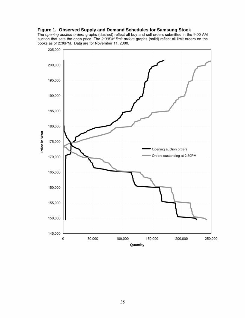
[Figure 1 about here]

Figure 1 graphs the demand and supply schedules on November 11th 2000 of

Samsung, a large and heavily traded KSE listing. 6 These graphs are constructed by

horizontally summing all limit orders that would execute at each theoretical price. 7 The sum

of all buy orders that would execute at a given price P is the demand for Samsung at that

price. As the price is decreased, tick by tick, successively more buy limit orders join the

executable list so the demand curve reaches further to the right at lower prices. The sum of 5 The KSE was open Saturday mornings until December 5, 1998, so on Saturdays during that period the second elasticity is estimated at 11:30 AM instead of 2:30 PM. Dropping these observations does not qualitatively change any of our results. 6 We randomly choose 3 other stocks from large, medium and small capitalization groups. These graphs all resemble Figure 1. 7 In estimating the elasticity of demand and supply, we use limit orders only because market orders, by definition, do not specify prices.

10

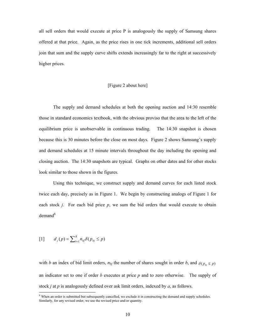
all sell orders that would execute at price P is analogously the supply of Samsung shares

offered at that price. Again, as the price rises in one tick increments, additional sell orders

join that sum and the supply curve shifts extends increasingly far to the right at successively

higher prices.

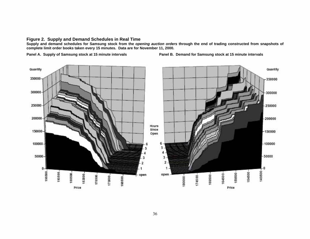
[Figure 2 about here]

The supply and demand schedules at both the opening auction and 14:30 resemble

those in standard economics textbook, with the obvious proviso that the area to the left of the

equilibrium price is unobservable in continuous trading. The 14:30 snapshot is chosen

because this is 30 minutes before the close on most days. Figure 2 shows Samsung’s supply

and demand schedules at 15 minute intervals throughout the day including the opening and

closing auction. The 14:30 snapshots are typical. Graphs on other dates and for other stocks

look similar to those shown in the figures.

Using this technique, we construct supply and demand curves for each listed stock

twice each day, precisely as in Figure 1. We begin by constructing analogs of Figure 1 for

each stock j. For each bid price p, we sum the bid orders that would execute to obtain

demand8

[1] )()(1

ppnpd bjB

b bjj ≤= ∑ =δ

with b an index of bid limit orders, nbj the number of shares sought in order b, and )( ppbj ≤δ

an indicator set to one if order b executes at price p and to zero otherwise. The supply of

stock j at p is analogously defined over ask limit orders, indexed by a, as follows. 8 When an order is submitted but subsequently cancelled, we exclude it in constructing the demand and supply schedules. Similarly, for any revised order, we use the revised price and/or quantity.

11

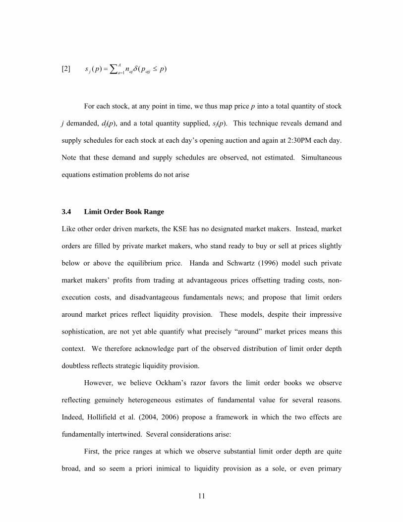
[2] )()(1

ppnps ajjA

a ajj ≤= ∑ =δ

For each stock, at any point in time, we thus map price p into a total quantity of stock

j demanded, dj(p), and a total quantity supplied, sj(p). This technique reveals demand and

supply schedules for each stock at each day’s opening auction and again at 2:30PM each day.

Note that these demand and supply schedules are observed, not estimated. Simultaneous

equations estimation problems do not arise

3.4 Limit Order Book Range

Like other order driven markets, the KSE has no designated market makers. Instead, market

orders are filled by private market makers, who stand ready to buy or sell at prices slightly

below or above the equilibrium price. Handa and Schwartz (1996) model such private

market makers’ profits from trading at advantageous prices offsetting trading costs, non-

execution costs, and disadvantageous fundamentals news; and propose that limit orders

around market prices reflect liquidity provision. These models, despite their impressive

sophistication, are not yet able quantify what precisely “around” market prices means this

context. We therefore acknowledge part of the observed distribution of limit order depth

doubtless reflects strategic liquidity provision.

However, we believe Ockham’s razor favors the limit order books we observe

reflecting genuinely heterogeneous estimates of fundamental value for several reasons.

Indeed, Hollifield et al. (2004, 2006) propose a framework in which the two effects are

fundamentally intertwined. Several considerations arise:

First, the price ranges at which we observe substantial limit order depth are quite

broad, and so seem a priori inimical to liquidity provision as a sole, or even primary

12

explanation. Table 2 shows substantial limit order depths beyond 5% away from the market

price – these represent about 34% and 33% of total limit buy and sell orders respectively. For

example, only 26% (24%) of total quantities demanded (supplied) fall within a one percent

range around the market price. The daily price fluctuation of a KSE stock exceeds 5% in

about 20% of days (across days when all four elasticities, demand and supply at open and

2:30PM, are measurable), so the tails of the limit order distribution, at least, point to

heterogeneous investor beliefs.

[Table 2 about here]

Second, Korea levies a 0.3% Tobin tax on all stock sales, even by brokers trading on

their own accounts. Public shareholders serving as liquidity providers confront even higher

transactions costs, for in 2000, brokerage fees ranged from 0.35% to 0.5%, though online

trading costs fell sharply after June 1998, and now range between 0.025% and 0.1%. Such

costs could deter limit orders solely to provide liquidity a costly strategy, but might just

spread liquidity-motivated limit orders further away from market prices.

Third, Table 1 shows market orders comprising only 5.22% of shares sought and

7.01% of shares offered. If limit orders existed primarily to provide liquidity, one might

expect them not to exceed market orders greatly, for the latter ought to include much of the

demand for quick execution. Aggregated limit order magnitudes, roughly sixteen to twenty-

fold greater than market orders at 2:30PM and seven to thirteen-fold greater at open, seem

superfluous. However, as noted above, current models of limit order strategies are hard to

quantify, so this argument can not be pressed to far.

These arguments are all incomplete, unquantifiable, and rightly discreditable as hand-

waving. Fortunately, Hollifield, Miller, Sandås, and Slive (2004, 2006) argue that

13

heterogeneous investor beliefs and liquidity provision are best considered jointly. In their

models, investors with heterogeneous beliefs place limit orders to capture their associated

quasirents and thereby provide liquidity. Their estimates suggest this interaction lets traders

with private information capture large fractions of its quasirents value, and thus encourages

their acquisition of costly private information (Grossman and Stiglitz, 1980). The provision

of liquidity is thus a by-product of heterogeneous investor information.

However, we concede that future research might alter our tentative conclusions if it

shows the sorts of limit order depth distributions we observe justified by liquidity provision

alone.

3.4. Elasticity Measurement Procedure

We measure elasticities by constructing analogs to Figure 1 for each stock twice each day. To

measure the elasticity of demand of firm j’s stock at a point in time, we regress total demand

at price pk on the log of pk,

[3] ( ) jkkjDjkj upbpd +−= lnln ,0 η

The elasticity of demand, jDη , is thus the percentage increase in quantity demanded due to a

one percent price rise, and so is minus one times the coefficient on ln pk in [3].

The elasticity of supply, jSη , is the percentage decrease in quantity supplied due to a

one percent price rise, and so is measured by the coefficient on the ln pk in [4].

[4] ( ) jkkjSjkj vpaps ++= lnln η

14

Both demand and supply elasticities are measured only when we have 5 or more

observations. In the final sample, the mean number of price-quantity pairs used is 19 for both

opening auction demand and supply elasticities, and 17 and 20 for 2:30 PM elasticities of

demand and supply, respectively. The average R2 numbers of regression [3] for opening and

2:30 PM are 73% and 66% and, those of [4] are 79% and 73% respectively.

Finally, although [3] and [4] use regression coefficients as elasticity measurements,

no simultaneity bias arises. This is because we are not jointly estimating supply and demand

curves from the same data. Rather, we are plotting out observed supply and demand curves

precisely and then using [3] and [4] to measure the slope of each curve.

4 Empirical Results

In this section, we first report patterns of demand and supply elasticities and then examine

firm-level daily panel regression. We divide our sample period into three sub-periods; a pre-

crisis period of December 1996 through October 1997, an in-crisis period of November 1997

to October 1998, and a post-crisis period of November 1998 to December 2000. 1997

November is chosen as the onset of the crisis, following Kim and Wei (2002).9

[Figure 3 about here]

4.1 Magnitudes

Panel A and B of Figure 3 plot the time series of daily mean elasticity measurements against

time. Table 3 reports the summary statistics of underlying firm level daily elasticities of

supply and demand curves. Table 3 shows that the median elasticities of demand and supply

9 On November, 1997, Bank of Korea stopped defending Korean Won and Korean government requested IMB bail-out.

15

curves are 20 and 22 respectively. A one percent increase in price thus causes roughly a 20

percent rise in demand and a 22 percent drop in supply.

Our elasticity measurements generally exceed the 10.50 figure imputed by Kaul et al.

(2000), the 7.89 estimate obtained by Wurgler and Zhuravskaya (2002), the mean (median)

elasticity of 0.68 (1.05) reported by Bagwell (1992) from Dutch auction share repurchases,

and the mean (median) estimates of 2.91 (2.47) by Kandel et al. (1999) from IPO data.

However, our estimate lies between the lower and upper bounds determined by Kalay et al.

(2004).

These differences might reflect the different methodologies used, the unique

information events used in some of the studies, different institutional arrangements in

different countries or time periods. For example, KSE investors observe quantities demanded

and supplied at the five best prices, whereas investors in other stock markets have less

information, sp higher average KSE elasticities are not entirely surprising.

We also check the differences between elasticities observed in opening auctions and

those observed at 2:30 PM. If uncertainty regarding private information were appreciably

resolved by trading, elasticities should rise through the day. Through our sample period, 2:30

PM mean elasticities generally exceed opening elasticities– consistent with Kalay et al.

(2004). However, our analogous median measurements show no discernable intraday pattern.

4.2 Harmony at Low Frequencies

One advantage of a long time series that includes a crisis is that in comparing elasticities

before and after the crisis using one measurement methodology. Thus, even if absolute

magnitudes are not directly comparable across studies, we can make valid comparisons over

time for Korea. The average elasticities of both supply and demand fluctuate far more during

the last months of 1997 and first months of 1998 than either before or after. This period of

16

instability corresponding to the onset of the 1997 Asian financial crisis, evident in the KSE

index in Panel A, is unsurprising.

More intriguingly, elasticities of both supply and demand are markedly lower after

this interlude of instability. Table 3 shows a 41% drop, from 29.7 to 17.6, in median demand

elasticity; and a 46% drop, from 35.8 to 19.6 in median supply elasticity. Similarly dramatic

reductions are evident in 2:30 PM measurements, and in the means of both measurements.

These differences are all statistically significant (p < 0.0001). Stocks valuations seem

significantly more heterogeneous after the crisis than before it. If so, the crisis permanently

altered both demand and supply curves. Note that even after the KSE market index reverts to

pre-crisis level, elasticities of both demand and supply curves for individual stocks remain

depressed. The drop-off is substantial – both persist at levels about 40% smaller after the

crisis than before it and neither reverses within our observation window.

Substantial fluctuation at higher frequencies is clearly superimposed on this step

function. However, no trend is evident within any of the subperiods. Higher frequency

fluctuations thus appear to approximate martingales.

These regularities suggest an underlying factor common to demand and supply

elasticities that follows a step function but otherwise changes little – varying little before or

after the crisis, but changing substantially during it. Possible candidates would be several

institutional reforms that have permanent impact. However, we can exclude them because

many of post-crisis reforms arguably rendered the country’s equity markets more transparent

and lowered arbitrage costs. Greater transparency should decrease information heterogeneity,

leaving both curves more elastic, all else equal. The advent of low-cost online trading after

June 1998, at first blush at least, should have reduced arbitrage costs and flattened supply and

demand curves. We return to these issues below.

17

In our sample, supply is generally more elastic than demand. The difference in means

is highly significant (p < 0.0001) throughout all three periods. Thus higher supply elasticities

are not artifacts of crisis fire-sales. Kalay et al. (2004) find supply less locally elastic (around

market prices) than demand for Tel Aviv stocks, and posit short sale constraints as an

explanation. Short sales are uncommon on the KSE, comprising only about 0.5% of pre-crisis

sell orders and an essentially negligible fraction post-crisis. Our relatively high supply

elasticities are thus not readily explained by more intense short sale activity in Korea than in

Tel Aviv..

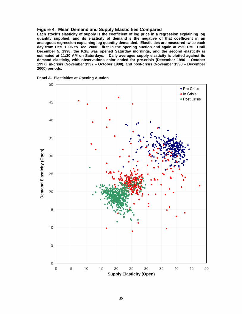
[Figures 4 and 5 about here]

4.2 Counterpoint at Higher Frequencies?

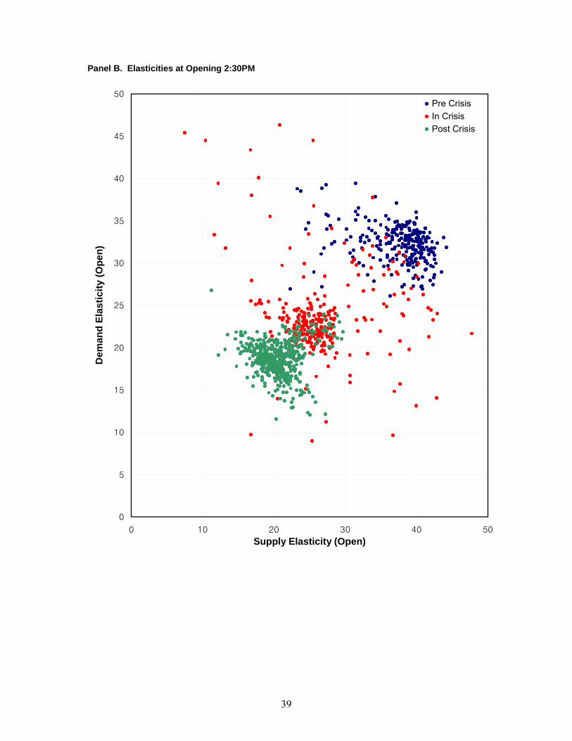
Figure 4 plots daily mean demand elasticities against daily mean supply elasticities for

individual stocks. Negative correlations amid much scatter are visible for both opening and

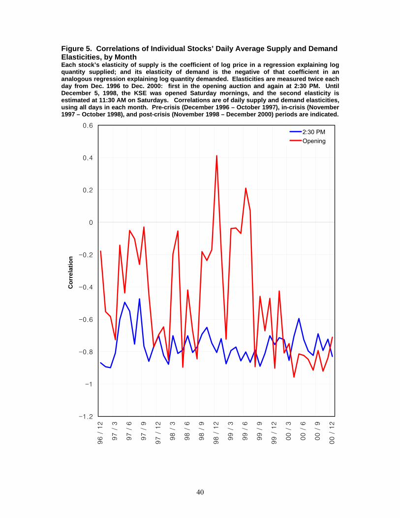
2:30PM measures. To confirm these visual patterns, we calculate correlations between the

two for each month. Figure 5 plots these against time, showing that they jibe roughly with the

intuition evident in Figure 4. The correlation of supply elasticity with demand elasticity is

usually negative in the opening auctions and is always markedly negative at 2:30PM. The

correlation of a stock’s demand elasticity and supply elasticity thus grows more negative

during the day. Moreover, while the 2:30 PM elasticities show a consistent negative

correlation throughout the sample period, the opening auction elasticities grow markedly

more negatively correlated later in the observation window – after the 1997 financial crisis.

4.3 Panel Regressions

18

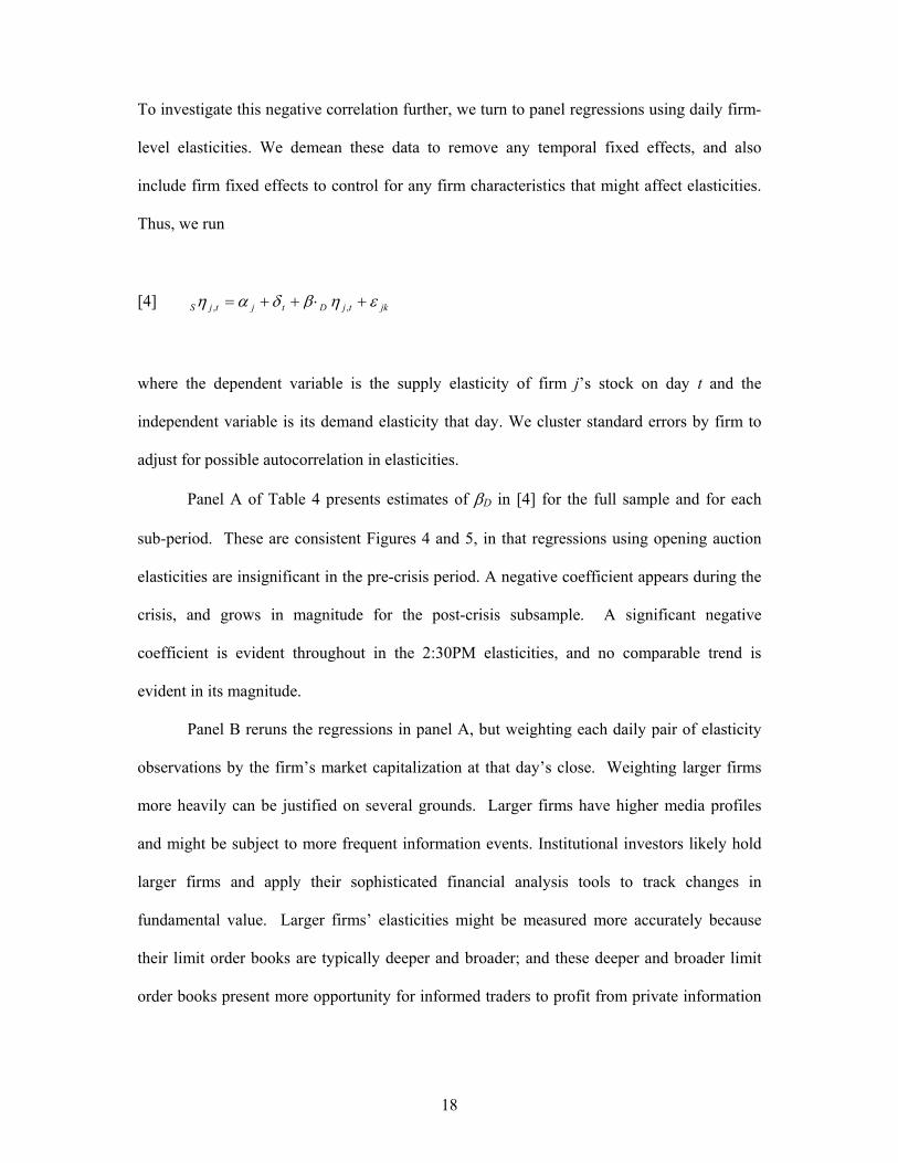
To investigate this negative correlation further, we turn to panel regressions using daily firm-

level elasticities. We demean these data to remove any temporal fixed effects, and also

include firm fixed effects to control for any firm characteristics that might affect elasticities.

Thus, we run

[4] jktjDtjtjS εηβδαη +⋅++= ,,

where the dependent variable is the supply elasticity of firm j’s stock on day t and the

independent variable is its demand elasticity that day. We cluster standard errors by firm to

adjust for possible autocorrelation in elasticities.

Panel A of Table 4 presents estimates of βD in [4] for the full sample and for each

sub-period. These are consistent Figures 4 and 5, in that regressions using opening auction

elasticities are insignificant in the pre-crisis period. A negative coefficient appears during the

crisis, and grows in magnitude for the post-crisis subsample. A significant negative

coefficient is evident throughout in the 2:30PM elasticities, and no comparable trend is

evident in its magnitude.

Panel B reruns the regressions in panel A, but weighting each daily pair of elasticity

observations by the firm’s market capitalization at that day’s close. Weighting larger firms

more heavily can be justified on several grounds. Larger firms have higher media profiles

and might be subject to more frequent information events. Institutional investors likely hold

larger firms and apply their sophisticated financial analysis tools to track changes in

fundamental value. Larger firms’ elasticities might be measured more accurately because

their limit order books are typically deeper and broader; and these deeper and broader limit

order books present more opportunity for informed traders to profit from private information

19

without immediately moving the price.10 Panel B replicates the negative correlations evident

in Panel A, and shows the progressively deepening negative correlations more starkly. The

open auction elasticities’ negative correlation deepens more: the coefficient is -0.004 in the

pre-crisis subsample and falls to -0.182 – about three times more negative than the analogous

coefficient in Panel A. The 2:30 PM elasticities now also show deepening negative

correlations – with a pre-crisis coefficient of -0.135 falling to -0.189 in the post-crisis

subperiod.

Our finding that individual stocks’ demand elasticities and supply elasticities are

contemporaneously negatively correlated survives a range of robustness checks. We cluster

standard errors by time, and obtain qualitatively similar results, by which we mean similar

patterns of signs and statistical significance to those in the tables. Running regressions in

first differences, rather than including firm fixed effects, controls for time-varying fixed

effects and also generates qualitatively similar results.

5. Towards an Interpretation

In this section, we start with a simple specification of demand (or supply) function as

discussed in Grossman and Stiglitz (1980) to guide our quest to find answers for empirical

results reported in the previous section. Grossman and Stiglitz (1980) derive the demand (or

supply) curve of investor i for a firm’s stock as

[5] i

ii V

PpD

α)( −

=

10 One alternative to this specification is to use interaction term. Results are qualitatively the same whether we use WLS or OLS with interaction terms.

20

with .ip the expected value investor i assigns to the stock, P its current market price, α the

risk aversion common to all investors, and iV the investor’s uncertainty about the stock’s

intrinsic value.

By assuming iV identical across investors and investors’ valuations .ip uniformly

distributed, the slope of aggregate demand curve can be written as

[6] VP

Dα1

−=∂∂

Under these simplifying assumptions, the demand (or supply) curve becomes steeper

if investors are more risk aversion or uncertainty about fundamental values, all else equal.

Wurgler and Zhuravskaya (2002) use a representation of this sort, in which V is also

interpreted as reflecting arbitrage risk. Absent uncertainty about fundamental value and

given perfectly homogeneous expectations across all investors, V approaches zero and the

curve becomes infinitely elastic. That is, all else equal, the lower the ambient risk aversion

and uncertainty about the fundamental value, the larger the price sensitivity of quantity

demanded or supplied.

This simple framework suggests that changes in either α or V might explain the post-

crisis depression in elasticities we observe. For example, if the crisis causes investors to

become more risk averse, perhaps because their wealth falls or because they become more

aware of volatility always intrinsic to equity investments, they become less willing to enter

large orders based on valuations differing from the market price. Thus an elevated α results

in smaller limit orders at each price and steepens supply and demand curves for individual

stocks, all else equal. Or, if the crisis made individual firms harder to value, perhaps by

overturning investors’ background assumptions or by inducing firms to pursue more

21

idiosyncratic and risky strategies, investors again become less enthusiastic about betting huge

amounts on their private valuations. Thus does greater uncertainty, a higher V, steepen

demand and supply curves for individual stocks, all else equal.

This sort of model thus goes far in explaining the long-run step function evident in

Figure 3. But to explain the negative correlation evident in Figures 4 and 5, we need to

address the strategic interactions between buyers and sellers. The theory literature offers little

guidance here, so we propose an intuitive framework and use it to motivate an exploratory

empirical study in the hope of spurring formal theory work.

Risk aversion and uncertainty as to fundamental value might also induce and

modulate the negative correlation as well. Kavajecz (1999) notes that specialists and limit

order traders both reduce depth around information events – possibly because they fear

trading against better informed investors. Thus, if private information that the stock is

overvalued solidifies in the hands of some investors, they enter large sell orders at and just

below the market price. This flattens the stock’s supply curve. If investors not party to this

private information observe such trades, they might mimic Kavajecz’s (1999) traders and

reduce their limit order depths for fear of trading at an informational disadvantage. All else

equal, this behavior steepens the demand curve of the affected stock. If the new private

information indicates that the stock is undervalued, the better informed investors enter large

limit orders to buy at or above the market price so everything works in reverse – flattening

the stock’s demand curve and steepening its supply curve This sort of reaction function

would induce the negative correlation between demand elasticity and supply elasticity we

observe at high frequencies. Roll (1988) argues that most information enters the market in

these ways – as private information gathered and interpreted by investors who trade on that

information for private gain.

22

The flattening due to large orders by investors with private information would

presumably be greater if they are less risk averse or more certain of their advantage. The

reactions by uninformed traders would presumably be stronger if they were more risk averse

or less sure of the validity of their valuations. A negative correlation between supply and

demand elasticities should thus be greatest when informed traders are more bold and certain

and uninformed traders more cautious and uncertain. Thus, a more prominent negative

correlation at 2:30 than at the open might indicate more information heterogeneity later in the

day, with privately informed traders growing more aggressive and uninformed traders

reacting with a more sever withdrawal of limit order depth.

To explore this admittedly highly speculative thesis, we require proxies for ambient

risk aversion, α, and uncertainty, V. We cannot readily gauge α from observed equity

premiums in this context, for Siegel and Thaler (1997) show that a financial crisis affects

both stock and bond markets, rendering the difference in average returns between them

problematic as a way of inferring α. One approach is to seek proxies. Thus, we might infer

changes in α from shifting patterns of investment. For example, a sudden flow of wealth from

tech stocks into government bonds might signal a newly elevated α, all else equal. We lack

data to track such shifts, but can construct some less direct proxy. In the following section,

we discuss the construction of proxies for α and V.

5. 1 Proxies for Uncertainty regarding Fundamental Values

This section motivates, critiques, and describes a set of variables plausibly related to

investors’ uncertainty as to stocks’ fundamental values. These are: the adverse selection

component of the bid-ask spread, a mean intraday price flux, and share turnover.

5.1.1 The Adverse Selection Component of the Bid-Ask Spread

23

The adverse selection component of the bid-ask spread is a popular measure of information

asymmetry between informed traders and liquidity providers in the microstructure literature.

Since asymmetric information increases as the uncertainty concerning firm value increases,

we conjecture that this variable to be positively related with V. Copeland and Galai (1983),

Glosten and Milgrom (1985), and Easley and O’Hara (1987) argue that liquidity traders often

sustain losses from trading with informed traders. Thus, liquidity providers include an

adverse selection cost in the bid-ask spreads they post. This lets them cover their expected

losses to informed traders.

The magnitude of this spread thus reflects liquidity traders’ perceptions of their

informational disadvantage, and thus of information heterogeneity in general. A larger bid-

ask spread should thus correlate with lower elasticities and a more negative correlation

between supply and demand elasticities.

To construct this measure, denoted spread, we decompose the observed spread – the

lowest ask, at, minus the highest bid, bt – into a realized half-spread and adverse selection

component as in Huang and Stoll (1996). 11 The former component gauges liquidity

providers’ post-trade earnings and the latter their losses to informed traders. We define

[7] ( )ttt ppspreadhalfrealized −=− +τλ

with pt the transaction price at time t, τ set to five minutes, and λt set to one for buy-initiated

trades and minus one for sell initiated trades.12 Because the spread depends on the tick size,

which depends on the price, we scale by the mid-point of the prevailing bid and ask. Thus,

we take the adverse selection component of the bid-ask spread as

11 In an order-driven market, it is not possible to place a buy (sell) order above (below) the prevailing lowest ask (highest bid) price. As a result, the effective spread is always the same as the quoted spread. 12 We have repeated the empirical analysis using τ = 30 minutes. This does not affect our results in any meaningful way.

24

[8] )(

)()(

21

tt

tttt

bappba

spread+

−−−≡ +τλ

.

5.1.2 Intraday Price Flux

Our second variable is intra-day price volatility. French and Roll (1986) and Roll (1988)

show most variation in individual stock returns to be firm-specific and unrelated to public

announcements. Roll (1988) argues that stock price movements are therefore largely caused

by investors trading on private firm-specific information. Higher volatility thus reflects more

active trading by informed arbitrageurs, and consequently a more heterogeneous distribution

of private information across investors. This, in turn, implies higher uncertainly about the

intrinsic value of firms to most investors, and thus less elastic demand and supply curves.

The same situation also implies a more severe reaction of uninformed investors to informed

traders, and thus a more prominent negative correlation between supply and demand

elasticities.

We estimate the intraday price flux, denoted volatility, for each stock each trading day

as the standard deviation of 5-minute price changes scaled by the mid-points of bid and ask

prices.

5.1.3 Share turnover

Our third proxy is share turnover. Trading occurs when investors disagree about

fundamental values (Karpoff, 1986). This presumably happens when different investors have

access to different private information – or draw different conclusions from common

information. Thus, trading volume measures the heterogeneity of expectations across

investors, so high volumes should accompany inelastic demand and supply curves. However,

25

high volume periods should also be periods of lower trading cost for arbitrageurs, and so of

more elastic demand and supply curves. Which effect dominates become an empirical

question.

We define turnover as shares traded divided by total shares outstanding.

5. 2 Proxies for Risk Aversion

We take the above three variables as proxies primarily reflecting the extent of information

heterogeneity, and now consider variables most directly linked to risk aversion. Obviously,

the first set might also be related to risk aversion. All else equal, more timorous market

makers should post higher spreads. All else equal, less risk averse investors should trade

more energetically on fainter information, perhaps elevating intraday flux and volume

measures. The variables to which we next turn might likewise be related to information

heterogeneity as well as risk aversion.

Impecunious individual investors can participate in the stock market by buying stocks

on margin or selling stocks short. Both procedures amount to borrowing money from

brokerage firms to trade securities, and thus increase an investor’s leverage. This necessarily

renders their portfolios riskier. For example, an investor who borrows money to buy a stock

can be in serious trouble if the stock price drops precipitously – unable to repay the loan by

selling the stock, she can face insolvency. To protect themselves from such situations,

brokers in Korea and elsewhere usually call in parts of such loans immediately if a stock’s

price drops. Margin trading became a popular fad among individual investors in the run-up

to the Asian Crisis. Deficient credit screening by brokers allowed legions of unsophisticated

and relatively shallow pocketed investors to trade on margin. When the crisis hit, prices

plummeted and many of these investors faced ruin. As a result, investors awareness of the

risks involved in margin trading rose.

26

To measure investor risk aversion, we use margin purchases as a fraction of total buy

limit orders and short sales as a fraction of total sell limit orders. We denote these variables

margin interest and short interest, respectively.

Several caveats are in order. First, changes in the costs of margin trading and short

sales might alter these measures absent any change investor risk aversion. During the crisis,

the cost of margin trading rose substantially as rapidly rising missed margin calls made

brokerage firms less generous with credit. In December 1997, the Korea Securities Finance

Corporation stopped lending to brokerage firms. 13 This cut the hypothecated credit the

brokers previously extended to investors, forcing them to hike collateral requirements from

140 percent to an average of 174 percent; and raise initial margin requirement as well. These

measures unquestionably raised both margin and short sales costs.

Although changes in either risk aversion or such costs should affect investors’ decisions to

buy on margin and sell short, the two have different predictions in the long run. Changes

due to altered tolerance for risk should persist after the crisis, whereas changes due to

elevated crisis-period trading costs should not as the costs of margin trading revert to pre-

crisis levels.

[Table 5 about here]

5.3 Low Frequency Results, Revisited

Elasticities of demand and supply drop markedly from the pre-crisis period to the post crisis

period, and our purpose in constructing the variables described above is to find factors that

display similar patterns. Table 5 presents summary statistics for each – first across the whole

sample period, and then for the pre-crisis, in-crisis, and post-crisis subperiods separately.

13 The Korea Securities Finance Corporation, established in October 1955, is the sole provider of securities finance services under the Securities and Exchange Act.

27

[Figures 6 and 7 about here]

The adverse selection component of the spread rises substantially, from 0.733 before

the crisis to 1.182 during it, but then falls to 0.696 after the crisis – a level lower than in the

pre-crisis period. This pattern, graphed in Figure 6, fails to track the step function in

elasticities also reproduced in that figure. Intraday price flux and share turnover both remain

elevated in the post-crisis period, though the price flux almost returns to pre-crisis levels.

Share turnover remains more substantially elevated, 2.41% in the post-crisis period versus

0.78% before the crisis, and its standard deviation is about sevenfold larger in the later

period. Figure 7 graphs both measures against time, and suggests share turnover as tracking

elasticities more faithfully than the other potential proxies for information asymmetry.

Further work is needed to assess the extent to which increased turnover reflects the reduced

transaction costs attendant to online trading, introduced in late 1990s.

[Figures 8 and 9 about here]

Figures 8 and 9 graph margin and short interest against time, and demonstrate a

marked and seemingly permanent drop in both during the crisis. Margin interest falls from

20.3% of buy limit orders before the crisis to only 1.3% in the post-crisis period. Short

interest drops from 1.3% of sell limit orders in the pre-crisis period to zero after it. Margin

lending was tightened substantially during the crisis, but most brokerage firms restored the

old rules by 1999.

28

Margin interest nonetheless remained markedly depressed. This is consistent with an

abrupt and persistent increase in risk aversion steepening both curves, though other

explanations are doubtless also possible

5.4 High Frequency Results, Revisited

Next, we revisit our finding of a negative correlation between a given stock’s elasticities of

supply and demand in daily data. To explore this further, we modify regression [6], including

interaction terms to see if the elasticities are more strongly negatively correlated when our

information heterogeneity proxies are larger. Here, we expect information heterogeneity

measures to dominate, since ambient risk aversion presumably changes little from day to day

(unless the composition of traders changes rapidly). We also exclude short interest from this

regression because it exhibits virtually no high frequency variation in the post-crisis

subperiod.

Our regression is thus

[8] jktjDttjDttjS X εηγηβδαη +⋅⋅+⋅++= − ,1,,

with Xt a vector containing the proxies for information asymmetry and risk aversion

developed above. Panel A and B of Table 6 report regressions analogous to those in Table 4.

[Table 6 about here]

The table clearly shows the increased negative correlation in the post-crisis subperiod

is a direct effect, not something mediated by the interaction terms. The magnitudes of βD, the

29

coefficient of ηD, shown in Table 6 differ little from those shown in Table 4. The interaction

terms also increase adjusted 2R very little.

Note also that the signs and significances of the interaction coefficients are quite

unstable across specifications. For example, in the post-crisis subperiod, the interaction of ηD

with volume attracts a negative coefficient in opening auction data, but is insignificant in

2:30PM data. The interaction with intraday flux is negative and significant in the equal-

weighted specifications using opening and 2:30 PM data, but becomes insignificant if

observations are weighted by market capitalization. The interaction with margin interest is

negative and significant regardless of the weighting, but only in 2:30 PM data. All these

results suggest an inconsistent magnification of the negative correlation between demand and

supply elasticities if information heterogeneity or risk aversion has increased. The interaction

with the adverse selection spread component, in contrast, attracts positive significant

coefficients – though for 2:30 PM data in equal-weighed regressions only. Taken at face

value, this might imply that the negative correlation is attenuated if market makers fear they

are at a worse informational disadvantage. Or, the adverse selection component might capture

‘general information’ uncertainty that affects both curves.

We believe the following best sums up these findings. Daily variation in plausible

proxies for neither information heterogeneity and risk aversion are terribly effective at

explaining neither daily variation in the magnitude of the negative correlation between a

stock’s supply and demand elasticities, nor the substantial rise in this negative correlation in

the post-crisis subperiod.

This is unsurprising as regards risk aversion, for this is a psychological parameter that

is unlikely to fluctuate greatly in the short run. Indeed, the persistently larger negative

correlations after the crisis suggest a link to ambient risk aversion, which plausibly also

remained elevated after the crisis. As regards information heterogeneity, whether our proxies

30

are inadequate or high frequency variation in information heterogeneity explains little of the

high frequency fluctuation in the negative correlation we observe.

5. Conclusions

The asset pricing literature descended from. Harrison and Kreps (1978) and Grossman and

Stiglitz (1980) posits finitely elastic demand and supply curves for individual stocks with

elasticities determined by the degree of information heterogeneity and investors’ risk

aversion. Blough (1988), Hindy (1989), De Long et al. (1990), Kandel and Peason (1992),

Harris and Raviv (1993), Varian (1985, 1989), Shleifer and Vishny (1997), and others all

elaborate theories along these lines, which in one way or another, all preserve the assumption

of finite elasticities.

We observe (not estimate) elasticities of the demand and supply curves of individual

stocks on the Korea Stock Exchange and find that these are unambiguously finite. Our

results thus validate the approach to asset pricing set forth in this literature.

The Asian financial crisis, which occurs midway through our sample window upset

conventional frameworks for understanding the Korean economy, and induced dramatic

changes in the business strategies of many Korean firms. Such factors may have increased the

heterogeneity of investors’ beliefs about fundamental values. The crisis also reduced the

wealth of many investors, and arguably also heightened their perceptions of the risks inherent

in equity – factors most readily interpreted as raising risk aversion among investors.

Information heterogeneity and investor risk aversion are both plausible determinants of the

elasticities or supply and demand curves for individual stocks in models permitting

heterogeneous investor perceptions of fundamental values.

Elasticities of both supply and demand are about 40% lower in the post-crisis period,

and do not revert within our observation window – although other financial and economic

31

indicators do return to their pre-crisis level. This is consistent with investors possessing

private information being less likely to enter large orders based on that information and with

liquidity providers fearing trading against better informed investors and therefore being more

cautious about providing limit order depth. However, common proxies used to reflect

information heterogeneity and risk aversion are of scant use in explaining this step function in

elasticities.

A stock’s elasticity of demand and elasticity of supply are robustly negatively

correlated in high frequency (daily) data. We speculate as to how informed investors entering

one side of the market with large orders would flatten one of the two curves, and how

uninformed investors on the other side, reacting to this, would withdraw limit order depth,

steepening the other curve. This negative correlation should again be larger if information

heterogeneity and risk aversion are larger. But once again, temporal variation in common

proxies for information heterogeneity and risk aversion is of scant use in explaining temporal

variation in the magnitude of this negative correlation.

Clearly, either our proxies are seriously flawed or other factors are complicating the

picture. We invite new theoretical models that might explain the robust empirical regularities

we detect.

References Bagwell, Laurie S., 1991, Shareholder heterogeneity: Evidence and implications, American Economic

Review 81, 218-221. Bagwell, Laurie S., 1992, Dutch auction repurchases: An analysis of shareholder heterogeneity,

Journal of Finance 47, 71-105. Baker, Malcolm and Serkan Savasoglu, 2002, Limited arbitrage in mergers and acquisitions, Journal

of Financial Economics 64, 91-116. Baker, Malcolm and Jeremy Stein, 2002, Market liquidity as a sentiment indicator, working paper,

Harvard University. Barber, Brad M. and Terrance Odean, 2000, Trading is hazardous to your wealth: The common stock

investment performance of individual investors, Journal of Finance 55, 773-806. Benartzi, Shlomo and Richard H. Thaler, 1995, Myopic loss aversion and the equity premium puzzle,

Quarterly Journal of Economics 110, 73-92.

32

Beneish, Messod, and Robert Whaley, 1996, An anatomy of the “S&P Game”: The effects of changing the rules, Journal of Finance 51, 1909-1930.

Black, Fischer, 1986, Noise, Journal of Finance 41, 529-543. Blough, S., 1988, Differences of opinion and the information value of prices, working paper, The

Johns Hopkins University. Blouinet, 2000 Bouchaud, Jean-Phillipe, Marc Mezard, and Marc Potters, 2002, Statistical properties of the stock

order books: Empirical results and models, Quantitative Finance 2, 251-256. Boz, Emine, 2007, Can miracle lead to crises? The role of optimism in emergin market crises,

Interntaional Monetary Fund working paper. Choe, Hyuk, Bong-Chan Kho, and René Stulz, 1999, Do foreign investors destabilize stock markets?

The Korean experience in 1997, Journal of Financial Economics 54, 227-254. Copeland, Thomas E. and Dan Galai, 1983, Information effects on the bid-ask spread, Journal of

Finance 38, 1457-1469. De Bondt, W. F. M. and Richard H. Thaler, 1985, Does the stock market overreact? Journal of

Finance 40, 793-805. De Long, J. Bradford, Andrei Shleifer, Lawrence H. Summers, and Robert J. Waldman, 1990, Noise

trader risk in financial markets, Journal of Political Economy 98, 703-738. Dhillon, Upinder, and Herb Johnson, 1991, Changes in the Standard and Poor’s 500 list, Journal of

Business 64, 75-85. Easley, David and Maureen O’Hara, 1987, Price, trade size, and information in securities markets,

Journal of Financial Economics 19, 69-90. Fama, 19xx Fama, Eugene and Kenneth French, 2007, Disagreement, tastes, and asset pricing, Journal of

Financial Economics 83, 667-689. French, Kenneth R. and Richard Roll, 1986, Stock return variances: the arrival of information and the

reaction of traders, Journal of Financial Economics 17, 5-26. Glosten, Lawrence, and Paul Milgrom, 1985, Bid, ask, and transaction prices in a specialist market

with heterogeneously informed traders, Journal of Financial Economics 13, 71-100. Greenwood, Robin,2005, Short- and long-term demand curves for stocks: theory and evidence on the

dynamics of arbitrage, Journal of Financial Economics 75 607-649. Grossman, Sanford and Joseph Stiglitz. 1980, On the impossibility of informationally efficient

markets, American Economic Review 70, 393-411. Handa, Puneet and Robert A. Schwartz, 1996, Limit order trading, Journal of Finance 51, 1835-1861. Harris, Lawrance and Eitan Gurel, 1986, Price and volume effects associated with changes in the S&P

500: New evidence for the existence of price pressures, Journal of Finance 41, 815-829. Harris, Milton and Artur Raviv, 1993, Differences of opinion make a horse race, Review of Financial

Studies 6, 473-506. Harrison, J. Michael and David M. Kreps, 1978, Speculative investor behavior in a stock market with

heterogeneous expectations, Quarterly Journal of Economics 93, 323-336. Hindy, A., 1989, An equilibrium model of futures markets dynamics, working paper, MIT. Hollifield, Burton, Robert A. Miller, and Patrik Sandás, 2004, Empirical analysis of limit order

markets, Review of Economic Studies 71, 1027-1063. Hollifield, Burton, Robert A. Miller, Patrik Sandás, and Joshua Slive, 2006, Estimating the gains from

trade in limit-order markets, Journal of Finance 61, 2753-2804. Huang, Roger, and Hans Stoll, 1996, Dealer versus auction markets: A paired comparison of

execution costs on NASDAQ and the NYSE, Journal of Financial Economics 41, 313-357. International Monetary Fund, 1998, World economic outlook: Financial crises: Causes and indicators,

World Economic and Financial Surves, Washington. Jain, Prem, 1987, The effect of stock price of inclusion in or exclusion from the S&P 500, Financial

Analysts Journal 43, 58-65. Kalay, Avner, Orly Sade, and Avi Wohl, 2004, Measuring stock illiquidity: An investigation of the

demand and supply schedules at the TASE, Journal of Financial Economics 74, 461-486.

33

Kandel, Eugene and Neil D. Pearson, 1995, Differential interpretation of public signals and trade in speculative markets, Journal of Political Economy 103, 831-872.

Kandel, Shmuel, Oded Sarig, and Avi Wohl, 1999, The demand for stocks: An analysis of IPO auctions, Review of Financial Studies 12, 227-247.

Karpoff, Jonathan M., 1986, A theory of trading volume, Journal of Finance 41, 1069-1088. Kaul, Aditya, Vikas Mehrotra, and Randall Morck, 2000, Demand curves for stocks do slope down:

New evidence from an index weights adjustment, Journal of Finance 55, 893-912. Kim, Woochan and Shang-Jin Wei, 2002, Foreign Portfolio Investors Before and During a Crisis

Journal of International Economics 56, No. 1, 77-96 Lintner, John. 1965. The valuation of risk assets and the selection of risky investments in stock

portfolios and capital budgets. Review of Economics and Statistics 47 13–37. Liu, Shinhua, 2000, Changes in the Nikkei 500: New evidence for downward sloping demand curves

for stocks, International Review of Finance 1, 245-267. Llorente, Guillermo, Roni Michaely, Gideon Saar and Jiang Wang, 2002, Dynamic volume-return

relations of individual stocks, Review of Financial Studies 15, 1005-1047. Lynch, Anthony, and Richard Mendenhall, 1997, New evidence on stock price effects associated with

changes in the S&P 500 Index, Journal of Business 70, 351-383. Markowitz, Harry, 1952, Portfolio selection, Journal of Finance 7, 77-91. Mikkelson, Wayne H. and M. Megan Partch, 1985, Stock price effects and costs of secondary

distributions, Journal of Financial Economics 14, 165-194. Mitchell, Mark, Todd Pulvino, and Erik Stafford, 2002, Limited arbitrage in equity markets, Journal

of Finance 57, 551-584. Newey, Whitney K. and Kenneth D. West, 1987, A simple, positive semi-definite, heteroskedasticity

and autocorrelation consistent covariance matrix, Econometrica 55, 703-708. Roll, Richard. 1988, R2, Journal of Finance 43, 541-566. Sharpe, William. 1964. Capital asset prices: A theory of market equilibrium under conditions of risk.

Journal of Finance 19 (3) 425-442 Scholes, Myron, 1972, The market for securities: Substitution versus price pressure and the effects of

information on share price, Journal of Business 45, 179-211. Shiller, Robert J., 2002, From efficient market theory to behavioral finance, Journal of Economic

Perspectives17, 83-104. Shiller, Robert J. and John Pound, 1989, Survey evidence on diffusion of interest and information

among investors, Journal of Economic Behavior and Organization 12, 47-66. Shleifer, Andrei, 1986, Do demand curves for stock slope down? Journal of Finance 41, 579-590. Shleifer, Andrei, 2000, Inefficient markets: An introduction to behavioral finance, Oxford University

Press Inc., New York. Shleifer, Andrei and Robert W. Vishny, 1997, The limits of arbitrage, Journal of Finance 52, 35-55. Siegel, Jeremy and Richard Thaler, 1997, Anomalies; The equity premium puzzle, Journal of

Economic Perspectives, 191-200. Tobin, James, 1958, Liquidity preference as behavior towards risk, Review of Economic Studies 25. Varian, Hal, 1985, Divergence of opinion in complete markets: A note, Journal of Finance 40, 309-

17. Varian, Hal, 1989, Differences of opinion in financial markets, in Courtenay C. Stone (ed.), Financial

Risk: Theory, Evidence and Implications, Proceedings of the Eleventh Annual Economic Policy Conference of the Federal Reserve Bank of St. Louis, Kluwer, Boston, 3-37.

Wang, Jiang, 1994, A model of competitive stock trading volume, Journal of Political Economy, 102, 127-168.

Wurgler, Jeffrey and Katia Zhuravskaya, 2002, Does arbitrage flatten demand curves for stocks?, Journal of Business 75, 583-608.

Zovko, Ilija and J. Doyne Farmer, 2002, The power of patience: A behavioral regularity in limit-order placement, Quantitative Finance 2, 387-392.

34

35

Figure 1. Observed Supply and Demand Schedules for Samsung Stock The opening auction orders graphs (dashed) reflect all buy and sell orders submitted in the 9:00 AM auction that sets the open price. The 2:30PM limit orders graphs (solid) reflect all limit orders on the books as of 2:30PM. Data are for November 11, 2000.

145,000

150,000

155,000

160,000

165,000

170,000

175,000

180,000

185,000

190,000

195,000

200,000

205,000

0 50,000 100,000 150,000 200,000 250,000

Quantity

Pric

e in

Won

Opening auction orders

Orders oustanding at 2:30PM

36

Figure 2. Supply and Demand Schedules in Real Time Supply and demand schedules for Samsung stock from the opening auction orders through the end of trading constructed from snapshots of complete limit order books taken every 15 minutes. Data are for November 11, 2000.

Panel A. Supply of Samsung stock at 15 minute intervals Panel B. Demand for Samsung stock at 15 minute intervals

37

Figure 3. Mean Demand and Supply Elasticities of Individual Stocks over Time Each stock’s elasticity of supply is the coefficient of log price in a regression explaining log quantity supplied; and its elasticity of demand s the negative of that coefficient in an analogous regression explaining log quantity demanded. Elasticities are measured twice each day from Dec. 1996 to Dec. 2000: first in the opening auction and again at 2:30 PM. Until December 5, 1998, the KSE was opened Saturday mornings, and the second elasticity is estimated at 11:30 AM on Saturdays. Daily elasticities are averaged across all stocks and then across days in specified periods: the entire sample, pre-crisis (December 1996 – October 1997), in-crisis (November 1997 – October 1998), and post-crisis (November 1998 – December 2000) periods. Upper panel shows KSE Composite Stock Price Index over this period

KSE Index Opening Auction Elasticities 2:30 PM Elasticities

38

Figure 4. Mean Demand and Supply Elasticities Compared Each stock’s elasticity of supply is the coefficient of log price in a regression explaining log quantity supplied; and its elasticity of demand s the negative of that coefficient in an analogous regression explaining log quantity demanded. Elasticities are measured twice each day from Dec. 1996 to Dec. 2000: first in the opening auction and again at 2:30 PM. Until December 5, 1998, the KSE was opened Saturday mornings, and the second elasticity is estimated at 11:30 AM on Saturdays. Daily averages supply elasticity is plotted against its demand elasticity, with observations color coded for pre-crisis (December 1996 – October 1997), in-crisis (November 1997 – October 1998), and post-crisis (November 1998 – December 2000) periods. Panel A. Elasticities at Opening Auction

0

5

10

15

20

25

30

35

40

45

50

0 5 10 15 20 25 30 35 40 45 50

Supply Elasticity (Open)

Dem

and

Elas

ticity

(Ope

n)

Pre CrisisIn CrisisPost Crisis

39

Panel B. Elasticities at Opening 2:30PM

0

5

10

15

20

25

30

35

40

45

50

0 10 20 30 40 50

Supply Elasticity (Open)

Dem

and

Elas

ticity

(Ope

n)Pre CrisisIn CrisisPost Crisis

40

Figure 5. Correlations of Individual Stocks’ Daily Average Supply and Demand Elasticities, by Month Each stock’s elasticity of supply is the coefficient of log price in a regression explaining log quantity supplied; and its elasticity of demand is the negative of that coefficient in an analogous regression explaining log quantity demanded. Elasticities are measured twice each day from Dec. 1996 to Dec. 2000: first in the opening auction and again at 2:30 PM. Until December 5, 1998, the KSE was opened Saturday mornings, and the second elasticity is estimated at 11:30 AM on Saturdays. Correlations are of daily supply and demand elasticities, using all days in each month. Pre-crisis (December 1996 – October 1997), in-crisis (November 1997 – October 1998), and post-crisis (November 1998 – December 2000) periods are indicated.

-1.2

-1

-0.8

-0.6

-0.4

-0.2

0

0.2

0.4

0.6

96 /

12

97 /

3

97 /

6

97 /

9

97 /

12

98 /

3

98 /

6

98 /

9

98 /

12

99 /

3

99 /

6

99 /

9

99 /

12

00 /

3

00 /

6

00 /

9

00 /

12

Cor

rela

tion

2:30 PMOpening

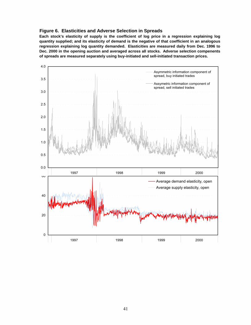
41

Figure 6. Elasticities and Adverse Selection in Spreads Each stock’s elasticity of supply is the coefficient of log price in a regression explaining logquantity supplied; and its elasticity of demand is the negative of that coefficient in an analogousregression explaining log quantity demanded. Elasticities are measured daily from Dec. 1996 toDec. 2000 in the opening auction and averaged across all stocks. Adverse selection compenentsof spreads are measured separately using buy-initiated and sell-initiated transaction prices.

0

20

40

60

1997 1998 1999 2000

Average demand elasticity, openAverage supply elasticity, open

0.0

0.5

1.0

1.5

2.0

2.5

3.0

3.5

4.0

1997 1998 1999 2000

Asymmetric information component ofspread, buy initiated trades

Assymetric information component ofspread, sell initiated trades

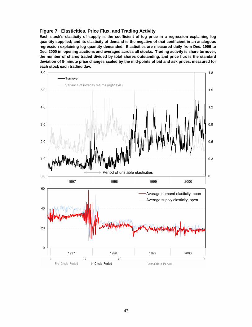
42

Figure 7. Elasticities, Price Flux, and Trading Activity Each stock’s elasticity of supply is the coefficient of log price in a regression explaining logquantity supplied; and its elasticity of demand is the negative of that coefficient in an analogousregression explaining log quantity demanded. Elasticities are measured daily from Dec. 1996 toDec. 2000 in opening auctions and averaged across all stocks. Trading activity is share turnover,the number of shares traded divided by total shares outstanding, and price flux is the standarddeviation of 5-minute price changes scaled by the mid-points of bid and ask prices, measured foreach stock each trading day.

0

20

40

60

1997 1998 1999 2000

Average demand elasticity, openAverage supply elasticity, open

0.0

1.0

2.0

3.0

4.0

5.0

6.0

1997 1998 1999 20000

0.3

0.6

0.9

1.2

1.5

1.8Turnover

Variance of intraday returns (right axis)

Period of unstable elasticities

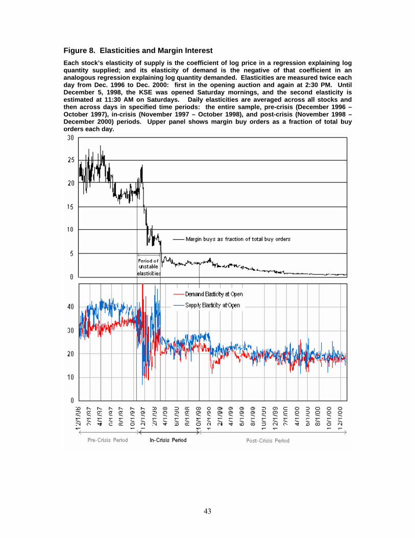
43

Figure 8. Elasticities and Margin Interest Each stock’s elasticity of supply is the coefficient of log price in a regression explaining log quantity supplied; and its elasticity of demand is the negative of that coefficient in an analogous regression explaining log quantity demanded. Elasticities are measured twice each day from Dec. 1996 to Dec. 2000: first in the opening auction and again at 2:30 PM. Until December 5, 1998, the KSE was opened Saturday mornings, and the second elasticity is estimated at 11:30 AM on Saturdays. Daily elasticities are averaged across all stocks and then across days in specified time periods: the entire sample, pre-crisis (December 1996 – October 1997), in-crisis (November 1997 – October 1998), and post-crisis (November 1998 – December 2000) periods. Upper panel shows margin buy orders as a fraction of total buy orders each day.

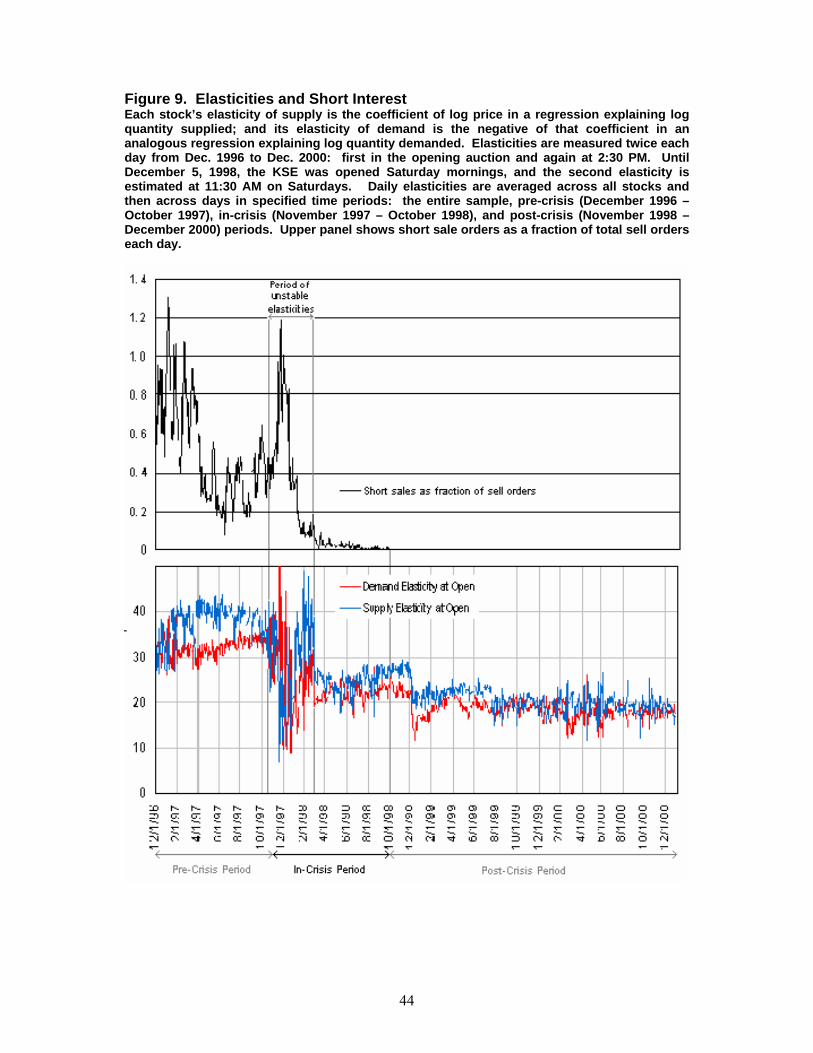
44

Figure 9. Elasticities and Short Interest Each stock’s elasticity of supply is the coefficient of log price in a regression explaining log quantity supplied; and its elasticity of demand is the negative of that coefficient in an analogous regression explaining log quantity demanded. Elasticities are measured twice each day from Dec. 1996 to Dec. 2000: first in the opening auction and again at 2:30 PM. Until December 5, 1998, the KSE was opened Saturday mornings, and the second elasticity is estimated at 11:30 AM on Saturdays. Daily elasticities are averaged across all stocks and then across days in specified time periods: the entire sample, pre-crisis (December 1996 – October 1997), in-crisis (November 1997 – October 1998), and post-crisis (November 1998 – December 2000) periods. Upper panel shows short sale orders as a fraction of total sell orders each day.

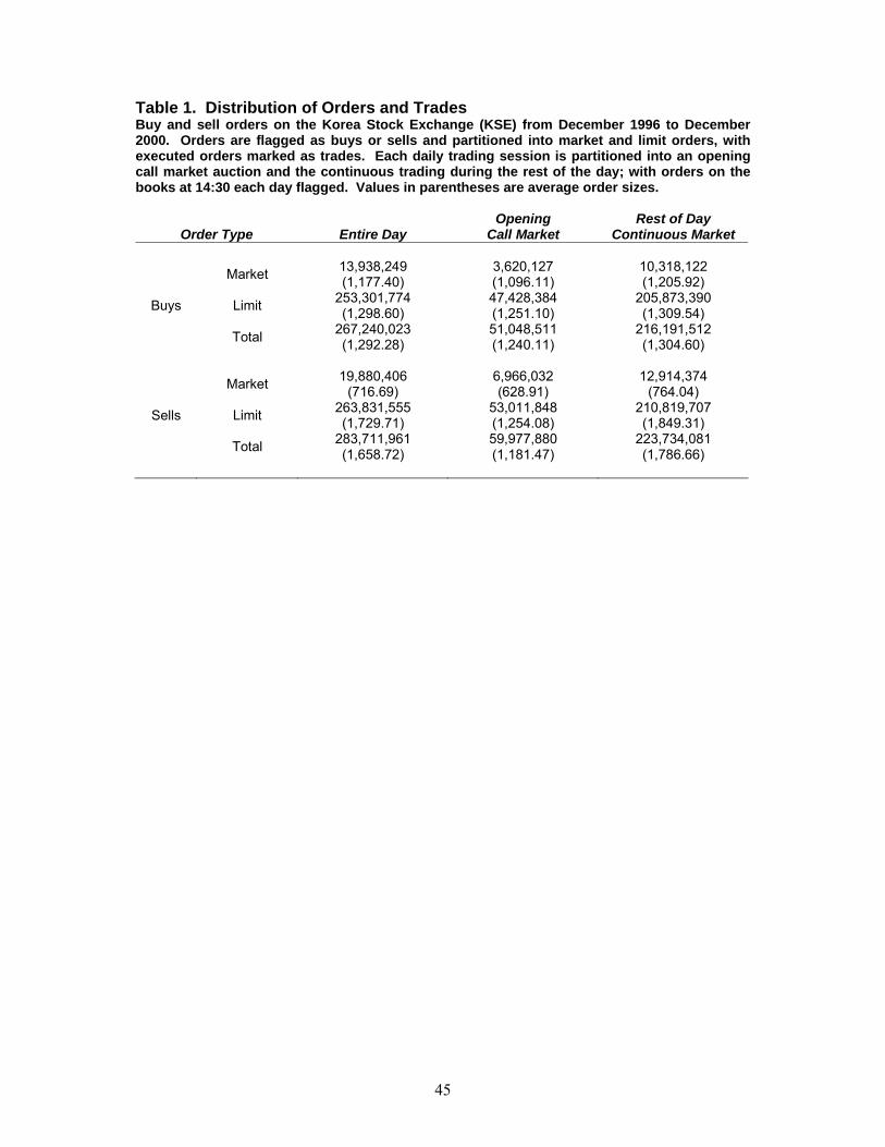
45

Table 1. Distribution of Orders and Trades Buy and sell orders on the Korea Stock Exchange (KSE) from December 1996 to December 2000. Orders are flagged as buys or sells and partitioned into market and limit orders, with executed orders marked as trades. Each daily trading session is partitioned into an opening call market auction and the continuous trading during the rest of the day; with orders on the books at 14:30 each day flagged. Values in parentheses are average order sizes.

Order Type Entire Day

Opening Call Market

Rest of Day Continuous Market

Market 13,938,249 (1,177.40)

3,620,127 (1,096.11)

10,318,122 (1,205.92)

Limit 253,301,774 (1,298.60)

47,428,384 (1,251.10)

205,873,390 (1,309.54) Buys

Total 267,240,023 (1,292.28)

51,048,511 (1,240.11)

216,191,512 (1,304.60)

Market 19,880,406 (716.69)

6,966,032 (628.91)

12,914,374 (764.04)

Limit 263,831,555 (1,729.71)

53,011,848 (1,254.08)

210,819,707 (1,849.31) Sells

Total 283,711,961 (1,658.72)

59,977,880 (1,181.47)

223,734,081 (1,786.66)

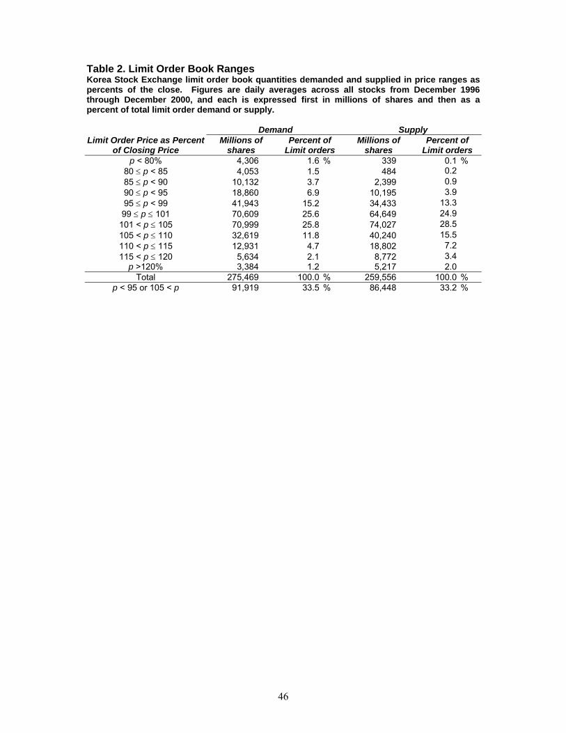
46

Table 2. Limit Order Book Ranges Korea Stock Exchange limit order book quantities demanded and supplied in price ranges as percents of the close. Figures are daily averages across all stocks from December 1996 through December 2000, and each is expressed first in millions of shares and then as a percent of total limit order demand or supply.

Demand Supply Limit Order Price as Percent

of Closing Price Millions of

shares Percent of

Limit orders Millions of

shares Percent of

Limit orders p < 80% 4,306 1.6 % 339 0.1 %

80 ≤ p < 85 4,053 1.5 484 0.2 85 ≤ p < 90 10,132 3.7 2,399 0.9 90 ≤ p < 95 18,860 6.9 10,195 3.9 95 ≤ p < 99 41,943 15.2 34,433 13.3 99 ≤ p ≤ 101 70,609 25.6 64,649 24.9

101 < p ≤ 105 70,999 25.8 74,027 28.5 105 < p ≤ 110 32,619 11.8 40,240 15.5 110 < p ≤ 115 12,931 4.7 18,802 7.2 115 < p ≤ 120 5,634 2.1 8,772 3.4

p >120% 3,384 1.2 5,217 2.0 Total 275,469 100.0 % 259,556 100.0 %

p < 95 or 105 < p 91,919 33.5 % 86,448 33.2 %

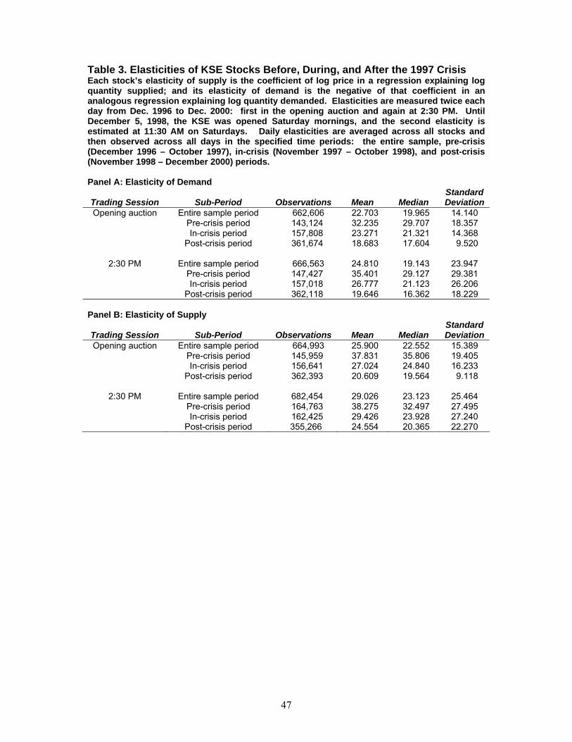
47

Table 3. Elasticities of KSE Stocks Before, During, and After the 1997 Crisis Each stock’s elasticity of supply is the coefficient of log price in a regression explaining log quantity supplied; and its elasticity of demand is the negative of that coefficient in an analogous regression explaining log quantity demanded. Elasticities are measured twice each day from Dec. 1996 to Dec. 2000: first in the opening auction and again at 2:30 PM. Until December 5, 1998, the KSE was opened Saturday mornings, and the second elasticity is estimated at 11:30 AM on Saturdays. Daily elasticities are averaged across all stocks and then observed across all days in the specified time periods: the entire sample, pre-crisis (December 1996 – October 1997), in-crisis (November 1997 – October 1998), and post-crisis (November 1998 – December 2000) periods. Panel A: Elasticity of Demand

Trading Session Sub-Period Observations Mean Median Standard Deviation

Opening auction Entire sample period 662,606 22.703 19.965 14.140 Pre-crisis period 143,124 32.235 29.707 18.357 In-crisis period 157,808 23.271 21.321 14.368 Post-crisis period 361,674 18.683 17.604 9.520

2:30 PM Entire sample period 666,563 24.810 19.143 23.947 Pre-crisis period 147,427 35.401 29.127 29.381 In-crisis period 157,018 26.777 21.123 26.206 Post-crisis period 362,118 19.646 16.362 18.229

Panel B: Elasticity of Supply

Trading Session Sub-Period Observations Mean Median Standard Deviation

Opening auction Entire sample period 664,993 25.900 22.552 15.389 Pre-crisis period 145,959 37.831 35.806 19.405 In-crisis period 156,641 27.024 24.840 16.233 Post-crisis period 362,393 20.609 19.564 9.118

2:30 PM Entire sample period 682,454 29.026 23.123 25.464 Pre-crisis period 164,763 38.275 32.497 27.495 In-crisis period 162,425 29.426 23.928 27.240 Post-crisis period 355,266 24.554 20.365 22.270

48

Table 4. Panel Regressions of Daily Observations of Stocks’ Supply Elasticities on their Demand Elasticities Each stock’s elasticity of supply is the coefficient of log price in a regression explaining log quantity supplied; and its elasticity of demand is the negative of that coefficient in an analogous regression explaining log quantity demanded. Elasticities are measured daily in opening auctions and at 14:30, 30 minutes before the close. Until December 5, 1998, the KSE was opened Saturdays until noon, so the second elasticity is measured at 11:30 those days. The sample is partitioned into pre-crisis (Dec. 1996 – Oct. 1997), in-crisis (Nov. 1997 – Oct. 1998), and post-crisis (Nov. 1998 – Dec. 2000) periods. The dependent variable is supply elasticity. The independent variable is demand elasticity. To remove any time effects, both daily elasticities are demeaned, and firm fixed effects remove any influence of persistent firm-level characteristics. Panel A reports equal-weighted panel regressions first for opening and then for 2:30 PM elasticities for the full sample period and also for each subperiod. Panel B reports analogous results but in panel regressions weighting observations by firm market capitalization. Numbers in parentheses are probability levels adjusted for firm clustering. Panel A: Equal-weighted panel estimation with time and firm fixed effects and firm clustered standard errors

Elasticities estimated in opening auctions Full window Pre-Crisis In-Crisis Post-Crisis

Estimate of βD -0.015 -0.003 -0.020 -0.053 Prob. βD = 0 (0.000) (0.348) (0.000) (0.000) Adjusted R2 0.024 0.048 0.050 0.046

Observations 601,042 115,280 132,799 352,963 Elasticities estimated in continuous trading at 2:30 PM Full window Pre-Crisis In-Crisis Post-Crisis

Estimate of βD -0.145 -0.150 -0.158 -0.144 Prob. βD = 0 (0.000) (0.000) (0.000) (0.000) Adjusted R2 0.024 0.041 0.035 0.025

Observations 593,248 126,506 125,115 341,627

Panel B: Market capitalization-weighted panel estimation with time and firm fixed effects and firm clustered standard errors

Elasticities estimated in opening auctions Full window Pre-Crisis In-Crisis Post-Crisis

Estimate of βD -0.048 -0.004 0.029 -0.182 Prob. βD = 0 (0.000) (0.733) (0.241) (0.000) Adjusted R2 0.023 0.031 0.040 0.081

Observations 597,911 114,780 132,729 350,402 Elasticities estimated in continuous trading at 2:30 PM Full window Pre-Crisis In-Crisis Post-Crisis

Estimate of βD -0.148 -0.135 -0.142 -0.189 Prob. βD = 0 (0.000) (0.000) (0.000) (0.000) Adjusted R2 0.023 0.051 0.023 0.031

Observations 589,175 125,936 124,969 338,270

49

Table 5. Information Heterogeneity and Risk Aversion Proxies The adverse selection component of the bid-ask spread is as in Huang and Stoll (1996), using either buy- or sell-initiated transaction prices. Intraday price flux is the standard deviation of 5-minute returns through the trading day. Share turnover is daily trading volume over shares outstanding. Margin interest is margin buy orders as a fraction of total buy orders; short interest is short sale orders as a fraction of total sell orders. All variables are estimated daily across the sample period, which is partitioned into three sub-periods: (a) pre-crisis period (December 1996 – October 1997), (b) in-crisis period (November 1997 – October 1998), and (c) post-crisis period (November 1998 – December 2000).

Sample Variable Sample Mean Median StandardDeviation

Adverse Selection Component of Spread 685,938 0.840 0.395 1.711

Share Turnover 804,089 1.607 0.642 6.670 Intraday Price Flux 776,552 0.661 0.573 0.477

Margin Interest 798,648 7.273 1.435 11.590

Full Sample

Short Interest 803,079 0.160 0.000 1.348

Adverse Selection Component of Spread 169,738 0.773 0.479 1.135

Share Turnover 201,383 0.773 0.305 1.420

Intraday Price Flux 193,377 0.544 0.504 0.293

Margin Interest 199,210 20.349 20.000 14.215

Pre-Crisis Period

Short Interest 201,064 0.480 0.000 2.313

Adverse Selection Component of Spread 175,817 1.182 0.546 2.251

Share Turnover 222,260 0.991 0.431 1.797 Intraday Price Flux 205,506 0.801 0.706 0.583

Margin Interest 219,184 5.760 2.500 8.705

In-Crisis Period

Short Interest 221,796 0.142 0.000 1.261

Adverse Selection Component of Spread 340,383 0.696 0.303 1.597

Share Turnover 380,446 2.408 1.125 9.478 Intraday Price Flux 377,669 0.644 0.555 0.469

Margin Interest 380,254 1.294 0.417 2.441

Post-Crisis Period

Short Interest 380,219 0.001 0.000 0.033

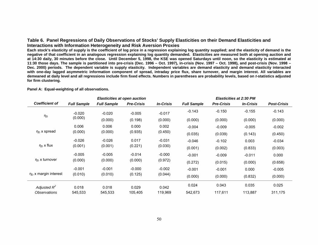
50

Table 6. Panel Regressions of Daily Observations of Stocks’ Supply Elasticities on their Demand Elasticities and Interactions with Information Heterogeneity and Risk Aversion Proxies Each stock’s elasticity of supply is the coefficient of log price in a regression explaining log quantity supplied; and the elasticity of demand is the negative of that coefficient in an analogous regression explaining log quantity demanded. Elasticities are measured both at opening auction and at 14:30 daily, 30 minutes before the close. Until December 5, 1998, the KSE was opened Saturdays until noon, so the elasticity is estimated at 11:30 those days. The sample is partitioned into pre-crisis (Dec. 1996 – Oct. 1997), in-crisis (Nov. 1997 – Oct. 1998), and post-crisis (Nov. 1998 – Dec. 2000) periods. The dependent variable is supply elasticity. Independent variables are demand elasticity and demand elasticity interacted with one-day lagged asymmetric information component of spread, intraday price flux, share turnover, and margin interest. All variables are demeaned at daily level and all regressions include firm fixed effects. Numbers in parentheses are probability levels, based on t-statistics adjusted for firm clustering. Panel A: Equal-weighting of all observations.

Elasticities at open auction Elasticities at 2:30 PM Coefficient of Full Sample Full Sample Pre-Crisis In-Crisis Full Sample Pre-Crisis In-Crisis Post-Crisis

-0.020 -0.020 -0.005 -0.017 -0.143 -0.150 -0.155 -0.143

ηD (0.000) (0.000) (0.198) (0.000) (0.000) (0.000) (0.000) (0.000)

0.006 0.006 0.000 0.002 -0.004 -0.009 -0.005 -0.002 ηD x spread (0.000)

(0.000) (0.935) (0.450) (0.035) (0.039) (0.143) (0.450)

-0.026 -0.026 0.017 -0.031 -0.046 -0.102 0.003 -0.034 ηD x flux (0.001)

(0.001) (0.221) (0.030) (0.001) (0.002) (0.833) (0.003)

-0.005 -0.005 -0.014 -0.000 -0.001 -0.009 -0.011 0.000 ηD x turnover (0.000)

(0.000) (0.000) (0.972) (0.272) (0.015) (0.000) (0.658)

-0.001 -0.001 -0.000 -0.002 -0.001 -0.001 0.000 -0.005 ηD x margin interest (0.010)

(0.010) (0.125) (0.044) (0.000) (0.000) (0.832) (0.000)

Adjusted R2 0.018 0.018 0.029 0.042 0.024 0.043 0.035 0.025

Observations 545,533 545,533 105,405 119,969 542,673 117,611 113,887 311,175

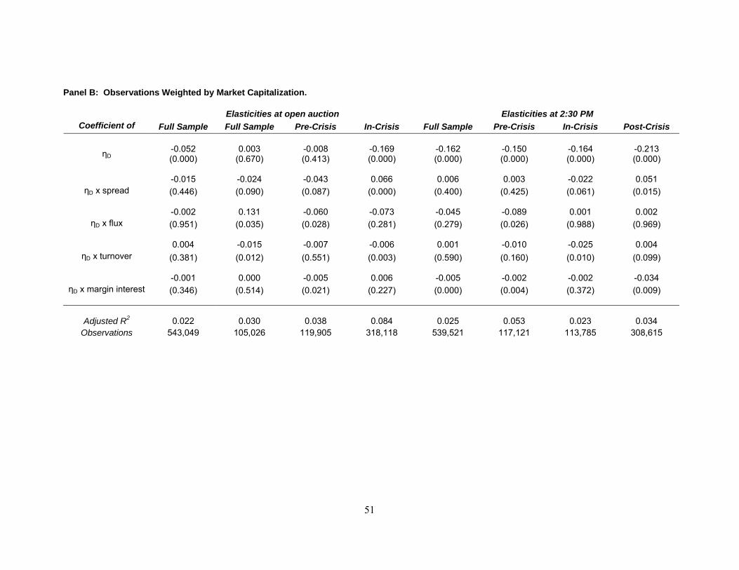
51

Panel B: Observations Weighted by Market Capitalization.

Elasticities at open auction Elasticities at 2:30 PM Coefficient of Full Sample Full Sample Pre-Crisis In-Crisis Full Sample Pre-Crisis In-Crisis Post-Crisis

-0.052 0.003 -0.008 -0.169 -0.162 -0.150 -0.164 -0.213 ηD (0.000)

(0.670) (0.413) (0.000) (0.000) (0.000) (0.000) (0.000)

-0.015 -0.024 -0.043 0.066 0.006 0.003 -0.022 0.051 ηD x spread (0.446)

(0.090) (0.087) (0.000) (0.400) (0.425) (0.061) (0.015)

-0.002 0.131 -0.060 -0.073 -0.045 -0.089 0.001 0.002 ηD x flux (0.951)

(0.035) (0.028) (0.281) (0.279) (0.026) (0.988) (0.969)

0.004 -0.015 -0.007 -0.006 0.001 -0.010 -0.025 0.004 ηD x turnover (0.381)

(0.012) (0.551) (0.003) (0.590) (0.160) (0.010) (0.099)

-0.001 0.000 -0.005 0.006 -0.005 -0.002 -0.002 -0.034 ηD x margin interest (0.346)

(0.514) (0.021) (0.227) (0.000) (0.004) (0.372) (0.009)

Adjusted R2 0.022 0.030 0.038 0.084 0.025 0.053 0.023 0.034

Observations 543,049 105,026 119,905 318,118 539,521 117,121 113,785 308,615