Doubly Robust Policy Evaluation and Optimization

arX

iv:1

503.

0283

4v1

[st

at.M

E]

10

Mar

201

5

Statistical Science

2014, Vol. 29, No. 4, 485–511DOI: 10.1214/14-STS500c© Institute of Mathematical Statistics, 2014

Doubly Robust Policy Evaluation and

Optimization1

Miroslav Dudık, Dumitru Erhan, John Langford and Lihong Li

Abstract. We study sequential decision making in environments whererewards are only partially observed, but can be modeled as a functionof observed contexts and the chosen action by the decision maker. Thissetting, known as contextual bandits, encompasses a wide variety ofapplications such as health care, content recommendation and Inter-net advertising. A central task is evaluation of a new policy given his-toric data consisting of contexts, actions and received rewards. The keychallenge is that the past data typically does not faithfully representproportions of actions taken by a new policy. Previous approaches relyeither on models of rewards or models of the past policy. The formerare plagued by a large bias whereas the latter have a large variance.In this work, we leverage the strengths and overcome the weaknesses

of the two approaches by applying the doubly robust estimation tech-nique to the problems of policy evaluation and optimization. We provethat this approach yields accurate value estimates when we have ei-ther a good (but not necessarily consistent) model of rewards or agood (but not necessarily consistent) model of past policy. Extensiveempirical comparison demonstrates that the doubly robust estimationuniformly improves over existing techniques, achieving both lower vari-ance in value estimation and better policies. As such, we expect thedoubly robust approach to become common practice in policy evalua-tion and optimization.

Key words and phrases: Contextual bandits, doubly robust estima-tors, causal inference.

1. INTRODUCTION

Contextual bandits (Auer et al., 2002/03; Lang-ford and Zhang, 2008), sometimes known as asso-

Miroslav Dudık is Senior Researcher and John Langfordis Principal Researcher, Microsoft Research, New York,New York, USA (e-mail: [email protected];[email protected]). Dumitru Erhan is Senior SoftwareEngineer, Google Inc., Mountain View, California, USAe-mail: [email protected]. Lihong Li is Researcher,Microsoft Research, Redmond, Washington, USAe-mail: [email protected].

1Parts of this paper were presented at the 28th Interna-tional Conference on Machine Learning (Dudık, Langford andLi, 2011), and the 28th Conference on Uncertainty in Artifi-cial Intelligence (Dudık et al., 2012).

ciative reinforcement learning (Barto and Anandan,1985), are a natural generalization of the classic mul-tiarmed bandits introduced by Robbins (1952). In acontextual bandit problem, the decision maker ob-serves contextual information, based on which anaction is chosen out of a set of candidates; in re-turn, a numerical “reward” signal is observed forthe chosen action, but not for others. The processrepeats for multiple steps, and the goal of the deci-sion maker is to maximize the total rewards in this

This is an electronic reprint of the original articlepublished by the Institute of Mathematical Statistics inStatistical Science, 2014, Vol. 29, No. 4, 485–511. Thisreprint differs from the original in pagination andtypographic detail.

1

http://arxiv.org/abs/1503.02834v1

http://www.imstat.org/sts/

http://dx.doi.org/10.1214/14-STS500

http://www.imstat.org

mailto:[email protected]




http://www.imstat.org

http://www.imstat.org/sts/

http://dx.doi.org/10.1214/14-STS500

2 DUDIK, ERHAN, LANGFORD AND LI

process. Usually, contexts observed by the decisionmaker provide useful information to infer the ex-pected reward of each action, thus allowing greaterrewards to be accumulated, compared to standardmulti-armed bandits, which take no account of thecontext.Many problems in practice can be modeled by con-

textual bandits. For example, in one type of Inter-net advertising, the decision maker (such as a web-site) dynamically selects which ad to display to auser who visits the page, and receives a paymentfrom the advertiser if the user clicks on the ad (e.g.,Chapelle and Li, 2012). In this case, the context canbe the user’s geographical information, the action isthe displayed ad and the reward is the payment. Im-portantly, we find only whether a user clicked on thepresented ad, but receive no information about theads that were not presented.Another example is content recommendation on

Web portals (Agarwal et al., 2013). Here, the deci-sion maker (the web portal) selects, for each uservisit, what content (e.g., news, images, videos andmusic) to display on the page. A natural objective isto “personalize” the recommendations, so that thenumber of clicks is maximized (Li et al., 2010). Inthis case, the context is the user’s interests in dif-ferent topics, either self-reported by the user or in-ferred from the user browsing history; the action isthe recommended item; the reward can be definedas 1 if the user clicks on an item, and 0 otherwise.Similarly, in health care, we only find out the clin-

ical outcome (the reward) of a patient who receiveda treatment (action), but not the outcomes for alter-native treatments. In general, the treatment strat-egy may depend on the context of the patient suchas her health level and treatment history. Therefore,contextual bandits can also be a natural model todescribe personalized treatments.The behavior of a decision maker in contextual

bandits can be described as a policy, to be de-fined precisely in the next sections. Roughly speak-ing, a policy is a function that maps the decisionmaker’s past observations and the contextual infor-mation to a distribution over the actions. This paperconsiders the offline version of contextual bandits:we assume access to historical data, but no abilityto gather new data (Langford, Strehl and Wortman,2008; Strehl et al., 2011). There are two relatedtasks that arise in this setting: policy evaluation andpolicy optimization. The goal of policy evaluationis to estimate the expected total reward of a given

policy. The goal of policy optimization is to obtaina policy that (approximately) maximizes expectedtotal rewards. The focus of this paper is on policyevaluation, but as we will see in the experiments,the ideas can also be applied to policy optimiza-tion. The offline version of contextual bandits is im-portant in practice. For instance, it allows a web-site to estimate, from historical log data, how muchgain in revenue can be achieved by changing the ad-selection policy to a new one (Bottou et al., 2013).Therefore, the website does not have to experimenton real users to test a new policy, which can be veryexpensive and time-consuming. Finally, we note thatthis problem is a special case of off-policy reinforce-ment learning (Precup, Sutton and Singh, 2000).Two kinds of approaches address offline policy

evaluation. The first, called the direct method (DM),estimates the reward function from given data anduses this estimate in place of actual reward toevaluate the policy value on a set of contexts.The second kind, called inverse propensity score(IPS) (Horvitz and Thompson, 1952), uses impor-tance weighting to correct for the incorrect pro-portions of actions in the historic data. The firstapproach requires an accurate model of rewards,whereas the second approach requires an accuratemodel of the past policy. In general, it might bedifficult to accurately model rewards, so the firstassumption can be too restrictive. On the otherhand, in many applications, such as advertising,Web search and content recommendation, the de-cision maker has substantial, and possibly perfect,knowledge of the past policy, so the second approachcan be applied. However, it often suffers from largevariance, especially when the past policy differs sig-nificantly from the policy being evaluated.In this paper, we propose to use the technique

of doubly robust (DR) estimation to overcomeproblems with the two existing approaches. Dou-bly robust (or doubly protected) estimation (Cas-sel, Sarndal and Wretman, 1976; Robins, Rot-nitzky and Zhao, 1994; Robins and Rotnitzky, 1995;Lunceford and Davidian, 2004; Kang and Schafer,2007) is a statistical approach for estimation fromincomplete data with an important property: if ei-ther one of the two estimators (i.e., DM or IPS)is correct, then the estimation is unbiased. Thismethod thus increases the chances of drawing re-liable inference.We apply the doubly robust technique to policy

evaluation and optimization in a contextual bandit

DOUBLY ROBUST POLICY EVALUATION AND OPTIMIZATION 3

setting. The most straightforward policies to con-sider are stationary policies, whose actions dependon the current, observed context alone. Nonstation-ary policies, on the other hand, map the current con-text and a history of past rounds to an action. Theyare of critical interest because online learning algo-rithms (also known as adaptive allocation rules), bydefinition, produce nonstationary policies. We ad-dress both stationary and nonstationary policies inthis paper.In Section 2, we describe previous work and con-

nect our setting to the related area of dynamic treat-ment regimes.In Section 3, we study stationary policy evalua-

tion, analyzing the bias and variance of our coretechnique. Unlike previous theoretical analyses, wedo not assume that either the reward model or thepast policy model are correct. Instead, we show howthe deviations of the two models from the truth im-pact bias and variance of the doubly robust estima-tor. To our knowledge, this style of analysis is noveland may provide insights into doubly robust esti-mation beyond the specific setting studied here. InSection 4, we apply this method to both policy eval-uation and optimization, finding that this approachcan substantially sharpen existing techniques.In Section 5, we consider nonstationary policy

evaluation. The main approach here is to use thehistoric data to obtain a sample of the run of anevaluated nonstationary policy via rejection sam-pling (Li et al., 2011). We combine the doubly ro-bust technique with an improved form of rejectionsampling that makes better use of data at the costof small, controllable bias. Experiments in Section 6suggest the combination is able to extract more in-formation from data than existing approaches.

2. PRIOR WORK

2.1 Doubly Robust Estimation

Doubly robust estimation is widely used in sta-tistical inference (see, e.g., Kang and Schafer, 2007,and the references therein). More recently, it hasbeen used in Internet advertising to estimate the ef-fects of new features for online advertisers (Lambertand Pregibon, 2007; Chan et al., 2010). Most of pre-vious analysis of doubly robust estimation is focusedon asymptotic behavior or relies on various model-ing assumptions (e.g., Robins, Rotnitzky and Zhao,1994; Lunceford and Davidian, 2004; Kang and

Schafer, 2007). Our analysis is nonasymptotic andmakes no such assumptions.Several papers in machine learning have used

ideas related to the basic technique discussed here,although not with the same language. For benignbandits, Hazan and Kale (2009) construct algo-rithms which use reward estimators to improveregret bounds when the variance of actual re-wards is small. Similarly, the Offset Tree algorithm(Beygelzimer and Langford, 2009) can be thoughtof as using a crude reward estimate for the “offset.”The algorithms and estimators described here aresubstantially more sophisticated.Our nonstationary policy evaluation builds on the

rejection sampling approach, which has been previ-ously shown to be effective (Li et al., 2011). Rela-tive to this earlier work, our nonstationary resultstake advantage of the doubly robust technique anda carefully introduced bias/variance tradeoff to ob-tain an empirical order-of-magnitude improvementin evaluation quality.

2.2 Dynamic Treatment Regimes

Contextual bandit problems are closely related todynamic treatment regime (DTR) estimation/opti-mization in medical research. A DTR is a set of (pos-sibly randomized) rules that specify what treatmentto choose, given current characteristics (includingpast treatment history and outcomes) of a patient.In the terminology of the present paper, the pa-tient’s current characteristics are contextual infor-mation, a treatment is an action, and a DTR is apolicy. Similar to contextual bandits, the quantityof interest in DTR can be expressed by a numericreward signal related to the clinical outcome of atreatment. We comment on similarities and differ-ences between DTR and contextual bandits in moredetail in later sections of the paper, where we de-fine our setting more formally. Here, we make a fewhigher-level remarks.Due to ethical concerns, research in DTR is of-

ten performed with observational data rather thanon patients. This corresponds to the offline ver-sion of contextual bandits, which only has accessto past data but no ability to gather new data.Causal inference techniques have been studied toestimate the mean response of a given DTR (e.g.,Robins, 1986; Murphy, van der Laan and Robins,2001), and to optimize DTR (e.g., Murphy, 2003;Orellana, Rotnitzky and Robins, 2010). These two


problems correspond to evaluation and optimizationof policies in the present paper.In DTR, however, a treatment typically exhibits a

long-term effect on a patient’s future “state,” whilein contextual bandits the contexts are drawn IIDwith no dependence on actions taken previously.Such a difference turns out to enable statisticallymore efficient estimators, which will be explained ingreater detail in Section 5.2.Despite these differences, as we will see later, con-

textual bandits and DTR share many similarities,and in some cases are almost identical. For exam-ple, analogous to the results introduced in this pa-per, doubly robust estimators have been applied toDTR estimation (Murphy, van der Laan and Robins,2001), and also used as a subroutine for optimizationin a family of parameterized policies (Zhang et al.,2012). The connection suggests a broader applica-bility of DTR techniques beyond the medical do-main, for instance, to the Internet-motivated prob-lems studied in this paper.

3. EVALUATION OF STATIONARY POLICIES

3.1 Problem Definition

We are interested in the contextual bandit settingwhere on each round:

1. A vector of covariates (or a context) x ∈ X isrevealed.

2. An action (or arm) a is chosen from a given setA.

3. A reward r ∈ [0,1] for the action a is revealed, butthe rewards of other actions are not. The rewardmay depend stochastically on x and a.

We assume that contexts are chosen IID from anunknown distribution D(x), the actions are chosenfrom a finite (and typically not too large) action setA, and the distribution over rewards D(r|a,x) doesnot change over time (but is unknown).The input data consists of a finite stream of triples

(xk, ak, rk) indexed by k = 1,2, . . . , n. We assumethat the actions ak are generated by some past (pos-sibly nonstationary) policy, which we refer to asthe exploration policy. The exploration history upto round k is denoted

zk = (x1, a1, r1, . . . , xk, ak, rk).

Histories are viewed as samples from a probabilitymeasure µ. Our assumptions about data generation

then translate into the assumption about factoringof µ as

µ(xk, ak, rk|zk−1)

=D(xk)µ(ak|xk, zk−1)D(rk|xk, ak),

for any k. Note that apart from the unknown dis-tribution D, the only degree of freedom above isµ(ak|xk, zk−1), that is, the unknown exploration pol-icy.When zk−1 is clear from the context, we use a

shorthand µk for the conditional distribution overthe kth triple

µk(x,a, r) = µ(xk = x,ak = a, rk = r|zk−1).

We also write Pµk and E

µk for Pµ[ · |zk−1] and

Eµ[ · |zk−1].Given input data zn, we study the stationary pol-

icy evaluation problem. A stationary randomizedpolicy ν is described by a conditional distributionν(a|x) of choosing an action on each context. Thegoal is to use the history zn to estimate the value ofν, namely, the expected reward obtained by follow-ing ν:

V (ν) =Ex∼DEa∼ν( · |x)Er∼D( · |x,a)[r].

In content recommendation on Web portals, for ex-ample, V (ν) measures the average click probabilityper user visit, one of the major metrics with criticalbusiness importance.In order to have unbiased policy evaluation, we

make a standard assumption that if ν(a|x)> 0 thenµk(a|x)> 0 for all k (and all possible histories zk−1).This clearly holds for instance if µk(a|x)> 0 for alla. Since ν is fixed in our paper, we will write Vfor V (ν). To simplify notation, we extend the con-ditional distribution ν to a distribution over triples(x,a, r)

ν(x,a, r) =D(x)ν(a|x)D(r|a,x)

and hence V =Eν [r].The problem of stationary policy evaluation, de-

fined above, is slightly more general than DTR anal-ysis in a typical cross-sectional observational study,where the exploration policy (known as “treatmentmechanism” in the DTR literature) is stationary;that is, the conditional distribution µ(ak|xk, zk−1)is independent of zk−1 and identical across all k,that is, µk = µ1 for all k.


3.2 Existing Approaches

The key challenge in estimating policy value incontextual bandits is that rewards are partially ob-servable: in each round, only the reward for the cho-sen action is revealed; we do not know what thereward would have been if we chose a different ac-tion. Hence, the data collected in a contextual ban-dit process cannot be used directly to estimate anew policy’s value: if in a context x the new policyselects an action a′ different from the action a cho-sen during data collection, we simply do not havethe reward signal for a′.There are two common solutions for overcom-

ing this limitation (see, e.g., Lambert and Pregibon,2007, for an introduction to these solutions). Thefirst, called the direct method (DM), forms an es-timate r(x,a) of the expected reward conditionedon the context and action. The policy value is thenestimated by

VDM =1

n

n∑

k=1

∑

a∈A

ν(a|xk)r(xk, a).

Clearly, if r(x,a) is a good approximation of thetrue expected reward ED[r|x,a], then the DM es-timate is close to V . A problem with this methodis that the estimate r is typically formed withoutthe knowledge of ν, and hence might focus on ap-proximating expected reward in the areas that areirrelevant for ν and not sufficiently in the areasthat are important for ν (see, e.g., the analysis ofBeygelzimer and Langford, 2009).The second approach, called inverse propensity

score (IPS), is typically less prone to problemswith bias. Instead of approximating the reward, IPSforms an approximation µk(a|x) of µk(a|x), and usesthis estimate to correct for the shift in action pro-portions between the exploration policy and the newpolicy:

VIPS =1

n

n∑

k=1

ν(ak|xk)µk(ak|xk)

· rk.

If µk(a|x) ≈ µk(a|x), then the IPS estimate abovewill be, approximately, an unbiased estimate of V .Since we typically have a good (or even accurate)understanding of the data-collection policy, it is of-ten easier to obtain good estimates µk, and thus theIPS estimator is in practice less susceptible to prob-lems with bias compared with the direct method.However, IPS typically has a much larger variance,

due to the increased range of the random variableν(ak|xk)/µk(ak|xk). The issue becomes more severewhen µk(ak|xk) gets smaller in high probability ar-eas under ν. Our approach alleviates the large vari-ance problem of IPS by taking advantage of the es-timate r used by the direct method.

3.3 Doubly Robust Estimator

Doubly robust estimators take advantage of boththe estimate of the expected reward r and theestimate of action probabilities µk(a|x). A sim-ilar idea has been suggested earlier by a num-ber of authors for different estimation problems(Cassel, Sarndal and Wretman, 1976; Rotnitzky andRobins, 1995; Robins and Rotnitzky, 1995; Murphy,van der Laan and Robins, 2001; Robins, 1998). Forthe setting in this section, the estimator of Murphy,van der Laan and Robins (2001) can be reduced to

VDR =1

n

n∑

k=1

[

r(xk, ν)(3.1)

+ν(ak|xk)µk(ak|xk)

· (rk − r(xk, ak))

]

,

where

r(x, ν) =∑

a∈A

ν(a|x)r(x,a)

is the estimate of Eν [r|x] derived from r. Informally,the doubly robust estimator uses r as a baseline andif there is data available, a correction is applied. Wewill see that our estimator is unbiased if at least oneof the estimators, r and µk, is accurate, hence thename doubly robust.In practice, quite often neither ED[r|x,a] or µk

is accurate. It should be noted that, although µk

tends to be much easier to estimate than ED[r|x,a]in applications that motivate this study, it is rareto be able to get a perfect estimator, due to engi-neering constraints in complex applications like Websearch and Internet advertising. Thus, a basic ques-tion is: How does the estimator VDR perform as theestimates r and µk deviate from the truth? The fol-lowing section analyzes bias and variance of the DRestimator as a function of errors in r and µk. Notethat our DR estimator encompasses DM and IPSas special cases (by respectively setting µk ≡∞ andr ≡ 0), so our analysis also encompasses DM andIPS.


3.4 Analysis

We assume that r(x,a) ∈ [0,1] and µk(a|x) ∈(0,∞], but in general µk does not need to repre-sent conditional probabilities (our notation is onlymeant to indicate that µk estimates µk, but no prob-abilistic structure). In general, we allow r and µk tobe random variables, as long as they satisfy the fol-lowing independence assumptions:

• r is independent of zn.• µk is conditionally independent of {(xℓ, aℓ, rℓ)}ℓ≥k,

conditioned on zk−1.

The first assumption means that r can be assumedfixed and determined before we see the input datazn, for example, by initially splitting the inputdataset and using the first part to obtain r and thesecond part to evaluate the policy. In our analysis,we condition on r and ignore any randomness in itschoice.The second assumption means that µk is not al-

lowed to depend on future. A simple way to satisfythis assumption is to split the dataset to form anestimator (and potentially also include data zk−1).If we have some control over the exploration pro-cess, we might also have access to “perfect logging”,that is, recorded probabilities µk(ak|xk). With per-fect logging, we can achieve µk = µk, respecting ourassumptions.2

Analogous to r(x,a), we define the populationquantity r∗(x,a)

r∗(x,a) =ED[r|x,a],and define r∗(x, ν) similarly to r(x, ν):

r∗(x, ν) =Eν [r|x].Let ∆(x,a) and k(x,a) denote, respectively, the

additive error of r and the multiplicative error of µk:

∆(x,a) = r(x,a)− r∗(x,a),

k(x,a) = µk(a|x)/µk(a|x).We assume that for some M ≥ 0, with probabilityone under µ:

ν(ak|xk)/µk(ak|xk)≤M

which can always be satisfied by enforcing µk ≥1/M .

2As we will see later in the paper, in order to reduce thevariance of the estimator it might still be advantageous to usea slightly inflated estimator, for example, µk = cµk for c > 1,or µk(a|x) =max{c,µk(a|x)} for some c > 0.

To bound the error of VDR, we first analyze a sin-gle term:

Vk = r(xk, ν) +ν(ak|xk)µk(ak|xk)

· (rk − r(xk, ak)).

We bound its range, bias, and conditional varianceas follows (for proofs, see Appendix A):

Lemma 3.1. The range of Vk is bounded as

|Vk| ≤ 1 +M.

Lemma 3.2. The expectation of the term Vk is

Eµk [Vk] = E

(x,a)∼ν[r∗(x,a) + (1− k(x,a))∆(x,a)].

Lemma 3.3. The variance of the term Vk can bedecomposed and bounded as follows:

Vµk [Vk](i)

= Vx∼D

[

Ea∼ν( · |x)

[r∗(x,a)

+ (1− k(x,a))

·∆(x,a)]]

− Ex∼D

[

Ea∼ν( · |x)

[k(x,a)∆(x,a)]2]

+ E(x,a)∼ν

[

ν(a|x)µk(a|x)

· k(x,a) · Vr∼D( · |x,a)

[r]

]

+ E(x,a)∼ν

[

ν(a|x)µk(a|x)

· k(x,a)∆(x,a)2]

.

Vµk [Vk](ii)

≤ Vx∼D

[r∗(x, ν)]

+ 2 E(x,a)∼ν

[|(1− k(x,a))∆(x,a)|]

+M E(x,a)∼ν

[

k(x,a)

· Er∼D( · |x,a)

[(r− r(x,a))2]]

.

The range of Vk is controlled by the worst-case ra-tio ν(ak|xk)/µk(ak|xk). The bias of Vk gets smalleras ∆ and k become more accurate, that is, as ∆≈ 0


and k ≈ 1. The expression for variance is more com-plicated. Lemma 3.3(i) lists four terms. The firstterm represents the variance component due to therandomness over x. The second term can contributeto the decrease in the variance. The final two termsrepresent the penalty due to the importance weight-ing. The third term scales with the conditional vari-ance of rewards (given contexts and actions), andit vanishes if rewards are deterministic. The fourthterm scales with the magnitude of ∆, and it cap-tures the potential improvement due to the use of agood estimator r.The upper bound on the variance [Lemma 3.3(ii)]

is easier to interpret. The first term is the varianceof the estimated variable over x. The second termmeasures the quality of the estimators µk and r—itequals zero if either of them is perfect (or if the unionof regions where they are perfect covers the supportof ν over x and a). The final term represents theimportance weighting penalty. It vanishes if we donot apply importance weighting (i.e., µk ≡∞ andk ≡ 0). With nonzero k, this term decreases witha better quality of r—but it does not disappear evenif r is perfect (unless the rewards are deterministic).

3.4.1 Bias analysis Lemma 3.2 immediately yieldsa bound on the bias of the doubly robust estima-tor, as stated in the following theorem. The specialcase for stationary policies (second part of the theo-rem) has been shown by Vansteelandt, Bekaert andClaeskens (2012).

Theorem 3.4. Let ∆ and k be defined asabove. Then the bias of the doubly robust estimatoris

|Eµ[VDR]− V |

=1

n

∣

∣

∣

∣

∣

Eµ

[

n∑

k=1

E(x,a)∼ν

[(1− k(x,a))∆(x,a)]

]∣

∣

∣

∣

∣

.

If the exploration policy µ and the estimator µk arestationary (i.e., µk = µ1 and µk = µ1 for all k), theexpression simplifies to

|Eµ[VDR]− V |= |Eν [(1− 1(x,a))∆(x,a)]|.Proof. The theorem follows immediately from

Lemma 3.2. �

In contrast, we have (for simplicity, assuming sta-tionarity of the exploration policy and its estimate)

|Eµ[VDM]− V |= |Eν [∆(x,a)]|,

|Eµ[VIPS]− V |= |Eν [r∗(x,a)(1− 1(x,a))]|,

where the first equality is based on the observationthat DM is a special case of DR with µk(a|x) ≡∞(and hence k ≡ 0), and the second equality is basedon the observation that IPS is a special case of DRwith r(x,a)≡ 0 (and hence ∆≡ r∗).In general, neither of the estimators dominates

the others. However, if either ∆ ≈ 0, or k ≈ 1,the expected value of the doubly robust estima-tor will be close to the true value, whereas DMrequires ∆ ≈ 0 and IPS requires k ≈ 1. Also, if‖k − 1‖p,ν ≪ 1 [for a suitable Lp(ν) norm], weexpect that DR will outperform DM. Similarly, ifk ≈ 1 but ‖∆‖p,ν ≪‖r∗‖p,ν , we expect that DR willoutperform IPS. Thus, DR can effectively take ad-vantage of both sources of information to lower thebias.

3.4.2 Variance analysis We argued that the ex-pected value of VDR compares favorably with IPSand DM. We next look at the variance of DR. Sincelarge-deviation bounds have a primary dependenceon variance; a lower variance implies a faster con-vergence rate. To contrast DR with IPS and DM,we study a simpler setting with a stationary explo-ration policy, and deterministic target policy ν, thatis, ν( · |x) puts all the probability on a single action.In the next section, we revisit the fully general set-ting and derive a finite-sample bound on the errorof DR.

Theorem 3.5. Let ∆ and k be defined asabove. If exploration policy µ and the estimator µk

are stationary, and the target policy ν is determinis-tic, then the variance of the doubly robust estimatoris

Vµ[VDR]

=1

n

(

V(x,a)∼ν

[r∗(x,a)

+ (1− 1(x,a))∆(x,a)]

+ E(x,a)∼ν

[

1

µ1(a|x)· 1(x,a) · V

r∼D( · |x,a)[r]

]

+ E(x,a)∼ν

[

1− µ1(a|x)µ1(a|x)

· 1(x,a)∆(x,a)2])

.

Proof. The theorem follows immediately fromLemma 3.3(i). �

The variance can be decomposed into three terms.The first term accounts for the randomness in x(note that a is deterministic given x). The other two


terms can be viewed as the importance weightingpenalty. These two terms disappear in DM, whichdoes not use rewards rk. The second term accountsfor randomness in rewards and disappears when re-wards are deterministic functions of x and a. How-ever, the last term stays, accounting for the disagree-ment between actions taken by ν and µ1.Similar expressions can be derived for the DM and

IPS estimators. Since IPS is a special case of DRwith r≡ 0, we obtain the following equation:

Vµ[VIPS]

=1

n

(

V(x,a)∼ν

[1(x,a)r∗(x,a)]

+ E(x,a)∼ν

[

1

µ1(a|x)· 1(x,a) · V

r∼D( · |x,a)[r]

]

+ E(x,a)∼ν

[

1− µ1(a|x)µ1(a|x)

· 1(x,a)r∗(x,a)2])

.

The first term will be of similar magnitude as thecorresponding term of the DR estimator, providedthat 1 ≈ 1. The second term is identical to the DRestimator. However, the third term can be muchlarger for IPS if µ1(a|x)≪ 1 and |∆(x,a)| is smallerthan r∗(x,a) for the actions chosen by ν.In contrast, for the direct method, which is a spe-

cial case of DR with µk ≡∞, the following varianceis obtained immediately:

Vµ[VDM] =1

nV

(x,a)∼ν[r∗(x,a) +∆(x,a)].

Thus, the variance of the direct method does nothave terms depending either on the exploration pol-icy or the randomness in the rewards. This factusually suffices to ensure that its variance is sig-nificantly lower than that of DR or IPS. However,as mentioned in the previous section, when we canestimate µk reasonably well (namely, k ≈ 1), thebias of the direct method is typically much larger,leading to larger errors in estimating policy values.

3.4.3 Finite-sample error bound By combiningbias and variance bounds, we now work out a spe-cific finite-sample bound on the error of the estima-tor VDR. While such an error bound could be usedas a conservative confidence bound, we expect it tobe too loose in most settings (as is typical for finite-sample bounds). Instead, our main intention is toexplicitly highlight how the errors of estimators rand µk contribute to the final error.

To begin, we first quantify magnitudes of the ad-ditive error ∆ = r − r∗ of the estimator r, and therelative error |1− k|= |µk − µk|/µk of the estima-tor µk:

Assumption 3.6. Assume there exist δ∆, δ ≥ 0such that

E(x,a)∼ν

[|∆(x,a)|]≤ δ∆,

and with probability one under µ:

|1− k(x,a)| ≤ δ for all k.

Recall that ν/µk ≤M . In addition, our analysisdepends on the magnitude of the ratio k = µk/µk

and a term that captures both the variance of therewards and the error of r.

Assumption 3.7. Assume there exist er, max ≥0 such that with probability one under µ, for all k:

E(x,a)∼ν

[

Er∼D( · |x,a)

[(r(x,a)− r)2]]

≤ er,

k(x,a)≤ max for all x,a.

With the assumptions above, we can now boundthe bias and variance of a single term Vk. As in theprevious sections, the bias decreases with the qualityof r and µk, and the variance increases with the vari-ance of the rewards and with the magnitudes of theratios ν/µk ≤M , µk/µk ≤ max. The analysis belowfor instance captures the bias-variance tradeoff ofusing µk ≈ cµk for some c > 1: such a strategy canlead to a lower variance (by lowering M and max)but incurs some additional bias that is controlled bythe quality of r.

Lemma 3.8. Under Assumptions 3.6–3.7, withprobability one under µ, for all k:

|Eµk [Vk]− V | ≤ δδ∆,

Vµk [Vk]≤Vx∼D[r

∗(x, ν)] + 2δδ∆ +Mmaxer.

Proof. The bias and variance bound followfrom Lemma 3.2 and Lemma 3.3(ii), respectively,by Holder’s inequality. �

Using the above lemma and Freedman’s inequalityyields the following theorem.

Theorem 3.9. Under Assumptions 3.6–3.7,with probability at least 1− δ,

|VDR − V |≤ δδ∆


+ 2max

{

(1 +M) ln(2/δ)

n,

√

(Vx∼D[r∗(x, ν)] + 2δδ∆ +Mmaxer) ln(2/δ)

n

}

.

Proof. The proof follows by Freedman’s in-equality (Theorem B.1 in Appendix B), applied to

random variables Vk, whose range and variance arebounded using Lemmas 3.1 and 3.8. �

The theorem is a finite-sample error bound thatholds for all sample size n, and in the limit theerror converges to δδ∆. As we mentioned, this re-sult gives a confidence interval for the doubly-robustestimate VDR for any finite sample n. Other au-thors have used asymptotic theory to derive con-fidence intervals for policy evaluation by showingthat the estimator is asymptotically normal (e.g.,Murphy, van der Laan and Robins, 2001; Zhanget al., 2012). When using asymptotic confidencebounds, it can be difficult to know a priori whetherthe asymptotic distribution has been reached,whereas our bound applies to all finite sample sizes.Although our bound may be conservative for smallsample sizes, it provides a “safe” nonasymptoticconfidence interval. In certain applications like thoseon the Internet, the sample size is usually largeenough for this kind of nonasymptotic confidencebound to be almost as small as its asymptotic value(the term δqδ∆ in Theorem 3.9), as demonstratedby Bottou et al. (2013) for online advertising.Note that Assumptions 3.6–3.7 rely on bounds of|1− k| and k which have to hold with probabilityone. In Appendix C, we replace these bounds withmoment bounds, and present analogs of Lemma 3.8and Theorem 3.9.

4. EXPERIMENTS: THE STATIONARY CASE

This section provides empirical evidence for theeffectiveness of the DR estimator compared to IPSand DM. We study these estimators on severalreal-world datasets. First, we use public bench-mark datasets for multiclass classification to con-struct contextual bandit data, on which we evalu-ate both policy evaluation and policy optimizationapproaches. Second, we use a proprietary datasetto model the pattern of user visits to an Internetportal. We study covariate shift, which can be for-malized as a special case of policy evaluation. Ourthird experiment uses another proprietary datasetto model slotting of various types of search resultson a webpage.

4.1 Multiclass Classification with Partial

Feedback

We begin with a description of how to turn a K-class classification dataset into a K-armed contex-tual bandit dataset. Instead of rewards, we will workwith losses, specifically the 0/1-classification error.The actions correspond to predicted classes. In theusual multiclass classification, we can infer the lossof any action on training data (since we know itscorrect label), so we call this a full feedback setting.On the other hand, in contextual bandits, we onlyknow the loss of the specific action that was taken bythe exploration policy, but of no other action, whichwe call a partial feedback setting. After choosing anexploration policy, our transformation from full topartial feedback simply “hides” the losses of actionsthat were not picked by the exploration policy.This protocol gives us two benefits: we can carry

out comparison using public multiclass classificationdatasets, which are more common than contextualbandit datasets. Second, fully revealed data can beused to obtain ground truth value of an arbitrarypolicy. Note that the original data is real-world, butexploration and partial feedback are simulated.

4.1.1 Data generation In a classification task, weassume data are drawn IID from a fixed distribution:(x, y) ∼ D, where x ∈ X is a real-valued covariatevector and y ∈ {1,2, . . . ,K} is a class label. A typ-ical goal is to find a classifier ν :X 7→ {1,2, . . . ,K}minimizing the classification error:

e(ν) = E(x,y)∼D

[I[ν(x) 6= y]],

where I[ · ] is an indicator function, equal to 1 if itsargument is true and 0 otherwise.The classifier ν can be viewed as a deterministic

stationary policy with the action set A= {1, . . . ,K}and the loss function

l(y, a) = I[a 6= y].

Loss minimization is symmetric to the reward max-imization (under transformation r= 1− l), but lossminimization is more commonly used in classifica-tion setting, so we work with loss here. Note thatthe distribution D(y|x) together with the definitionof the loss above, induce the conditional probabilityD(l|x,a) in contextual bandits, and minimizing theclassification error coincides with policy optimiza-tion.


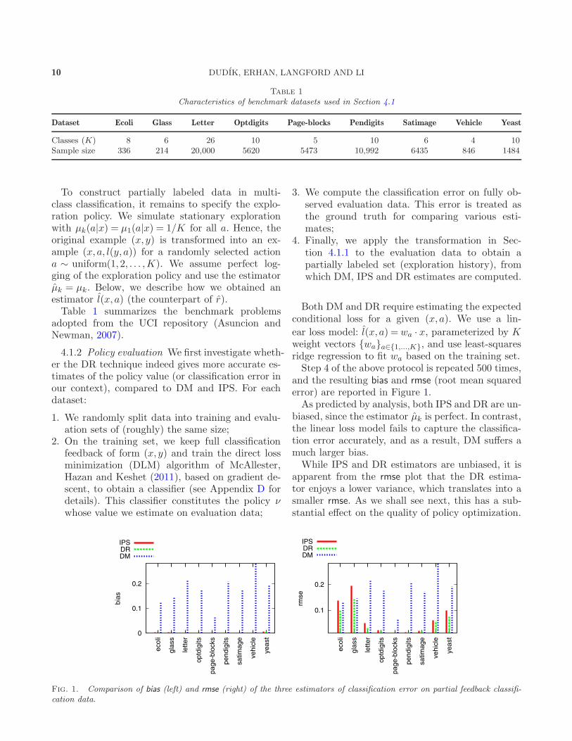
Table 1

Characteristics of benchmark datasets used in Section 4.1

Dataset Ecoli Glass Letter Optdigits Page-blocks Pendigits Satimage Vehicle Yeast

Classes (K) 8 6 26 10 5 10 6 4 10Sample size 336 214 20,000 5620 5473 10,992 6435 846 1484

To construct partially labeled data in multi-class classification, it remains to specify the explo-ration policy. We simulate stationary explorationwith µk(a|x) = µ1(a|x) = 1/K for all a. Hence, theoriginal example (x, y) is transformed into an ex-ample (x,a, l(y, a)) for a randomly selected actiona ∼ uniform(1,2, . . . ,K). We assume perfect log-ging of the exploration policy and use the estimatorµk = µk. Below, we describe how we obtained anestimator l(x,a) (the counterpart of r).Table 1 summarizes the benchmark problems

adopted from the UCI repository (Asuncion andNewman, 2007).

4.1.2 Policy evaluation We first investigate wheth-er the DR technique indeed gives more accurate es-timates of the policy value (or classification error inour context), compared to DM and IPS. For eachdataset:

1. We randomly split data into training and evalu-ation sets of (roughly) the same size;

2. On the training set, we keep full classificationfeedback of form (x, y) and train the direct lossminimization (DLM) algorithm of McAllester,Hazan and Keshet (2011), based on gradient de-scent, to obtain a classifier (see Appendix D fordetails). This classifier constitutes the policy νwhose value we estimate on evaluation data;

3. We compute the classification error on fully ob-served evaluation data. This error is treated asthe ground truth for comparing various esti-mates;

4. Finally, we apply the transformation in Sec-tion 4.1.1 to the evaluation data to obtain apartially labeled set (exploration history), fromwhich DM, IPS and DR estimates are computed.

Both DM and DR require estimating the expectedconditional loss for a given (x,a). We use a lin-

ear loss model: l(x,a) =wa · x, parameterized by Kweight vectors {wa}a∈{1,...,K}, and use least-squaresridge regression to fit wa based on the training set.Step 4 of the above protocol is repeated 500 times,

and the resulting bias and rmse (root mean squarederror) are reported in Figure 1.As predicted by analysis, both IPS and DR are un-

biased, since the estimator µk is perfect. In contrast,the linear loss model fails to capture the classifica-tion error accurately, and as a result, DM suffers amuch larger bias.While IPS and DR estimators are unbiased, it is

apparent from the rmse plot that the DR estima-tor enjoys a lower variance, which translates into asmaller rmse. As we shall see next, this has a sub-stantial effect on the quality of policy optimization.

Fig. 1. Comparison of bias (left) and rmse (right) of the three estimators of classification error on partial feedback classifi-cation data.


4.1.3 Policy optimization This subsection devi-

ates from much of the paper to study policy op-

timization rather than policy evaluation. Given a

space of possible policies, policy optimization is a

procedure that searches this space for the policy

with the highest value. Since policy values are un-

known, the optimization procedure requires access

to exploration data and uses a policy evaluator as

a subroutine. Given the superiority of DR over DM

and IPS for policy evaluation (in previous subsec-

tion), a natural question is whether a similar benefit

can be translated into policy optimization as well.

Since DM is significantly worse on all datasets, as

indicated in Figure 1, we focus on the comparison

between IPS and DR.

Here, we apply the data transformation in Sec-

tion 4.1.1 to the training data, and then learn a

classifier based on the loss estimated by IPS and

DR, respectively. Specifically, for each dataset, we

repeat the following steps 30 times:

1. We randomly split data into training (70%) and

test (30%) sets;

2. We apply the transformation in Section 4.1.1 to

the training data to obtain a partially labeled set

(exploration history);

3. We then use the IPS and DR estimators to im-

pute unrevealed losses in the training data; that

is, we transform each partial-feedback example

(x,a, l) into a cost sensitive example of the form

(x, l1, . . . , lK) where la′ is the loss for action a′,

imputed from the partial feedback data as fol-

lows:

la′ =

l(x,a′) +l− l(x,a′)

µ1(a′|x), if a′ = a,

l(x,a′), if a′ 6= a.

In both cases, µ1(a′|x) = 1/K (recall that µ1 =

µk); in DR we use the loss estimate (described

below), in IPS we use l(x,a′) = 0;4. Two cost-sensitive multiclass classification algo-

rithms are used to learn a classifier from thelosses completed by either IPS or DR: the firstis DLM used also in the previous section (seeAppendix D and McAllester, Hazan and Keshet,2011), the other is the Filter Tree reduction ofBeygelzimer, Langford and Ravikumar (2008)applied to a decision-tree base learner (see Ap-pendix E for more details);

5. Finally, we evaluate the learned classifiers on thetest data to obtain classification error.

Again, we use least-squares ridge regression tobuild a linear loss estimator: l(x,a) = wa · x. How-ever, since the training data is partially labeled, wa

is fitted only using training data (x,a′, l) for whicha= a′. Note that this choice slightly violates our as-sumptions, because l is not independent of the train-ing data zn. However, we expect the dependence tobe rather weak, and we find this approach to be morerealistic in practical scenarios where one might wantto use all available data to form the reward estima-tor, for instance due to data scarcity.Average classification errors (obtained in Step 5

above) of 30 runs are plotted in Figure 2. Clearly,for policy optimization, the advantage of the DR

Fig. 2. Classification error of direct loss minimization (left) and filter tree (right). Note that the representations used byDLM and the trees are very different, making any comparison between the two approaches difficult. However, the Offset Treeand Filter Tree approaches share a similar tree representation of the classifiers, so differences in performance are purely amatter of superior optimization.


is even greater than for policy evaluation. In alldatasets, DR provides substantially more reliableloss estimates than IPS, and results in significantlyimproved classifiers.Figure 2 also includes classification error of the

Offset Tree reduction (Beygelzimer and Langford,2009), which is designed specifically for policy opti-mization with partially labeled data.3 While the IPSversions of DLM and Filter Tree are rather weak, theDR versions are competitive with Offset Tree in alldatasets, and in some cases significantly outperformOffset Tree.Our experiments show that DR provides similar

improvements in two very different algorithms, onebased on gradient descent, the other based on treeinduction, suggesting the DR technique is gener-ally useful when combined with different algorithmicchoices.

4.2 Estimating the Average Number of User

Visits

The next problem we consider is estimating theaverage number of user visits to a popular Internetportal. We formulate this as a regression problemand in our evaluation introduce an artificial covari-ate shift. As in the previous section, the original datais real-world, but the covariate shift is simulated.Real user visits to the website were recorded for

about 4 million bcookies4 randomly selected fromall bcookies during March 2010. Each bcookie is as-sociated with a sparse binary covariate vector in5000 dimensions. These covariates describe brows-ing behavior as well as other information (suchas age, gender and geographical location) of thebcookie. We chose a fixed time window in March2010 and calculated the number of visits by eachselected bcookie during this window. To summa-rize, the dataset contains N = 3,854,689 data points:D = {(bi, xi, vi)}i=1,...,N , where bi is the ith (unique)bcookie, xi is the corresponding binary covariatevector, and vi is the number of visits (the response

3We used decision trees as the base learner in Offset Treesto parallel our base learner choice in Filter Trees. The num-bers reported here are not identical to those by Beygelzimerand Langford (2009), even though we used a similar protocolon the same datasets, probably because of small differencesin the data structures used.

4A bcookie is a unique string that identifies a user. Strictlyspeaking, one user may correspond to multiple bcookies, butfor simplicity we equate a bcookie with a user.

variable); we treat the empirical distribution over Das the ground truth.If it is possible to sample x uniformly at random

from D and measure the corresponding value v, thesample mean of v will be an unbiased estimate of thetrue average number of user visits, which is 23.8 inthis problem. However, in various situations, it maybe difficult or impossible to ensure a uniform sam-pling scheme due to practical constraints. Instead,the best that one can do is to sample x from someother distribution (e.g., allowed by the business con-straints) and measure the corresponding value v.In other words, the sampling distribution of x ischanged, but the conditional distribution of v givenx remains the same. In this case, the sample averageof v may be a biased estimate of the true quantityof interest. This setting is known as covariate shift(Shimodaira, 2000), where data are missing at ran-dom (see Kang and Schafer, 2007, for related com-parisons).Covariate shift can be modeled as a contextual

bandit problem with 2 actions: action a = 0 cor-responding to “conceal the response” and actiona = 1 corresponding to “reveal the response.” Be-low we specify the stationary exploration policyµk(a|x) = µ1(a|x). The contextual bandit data isgenerated by first sampling (x, v)∼D, then choos-ing an action a∼ µ1( · |x), and observing the rewardr = a · v (i.e., reward is only revealed if a= 1). Theexploration policy µ1 determines the covariate shift.The quantity of interest, ED[v], corresponds to thevalue of the constant policy ν which always chooses“reveal the response.”To define the exploration sampling probabilities

µ1(a = 1|x), we adopted an approach similar toGretton et al. (2008), with a bias toward the smallervalues along the first principal component of thedistribution over x. In particular, we obtained thefirst principal component (denoted x) of all covari-ate vectors {xi}i=1,...,N , and projected all data ontox. Let φ be the density of a univariate normaldistribution with mean m + (m −m)/3 and stan-dard deviation (m−m)/4, where m is the minimumand m is the mean of the projected values. We setµ1(a= 1|x) = min{φ(x · x),1}.To control the size of exploration data, we ran-

domly subsampled a fraction f ∈ {0.0001, 0.0005,0.001, 0.005, 0.01, 0.05} from the entire dataset Dand then chose actions a according to the explo-ration policy. We then calculated the IPS and DR


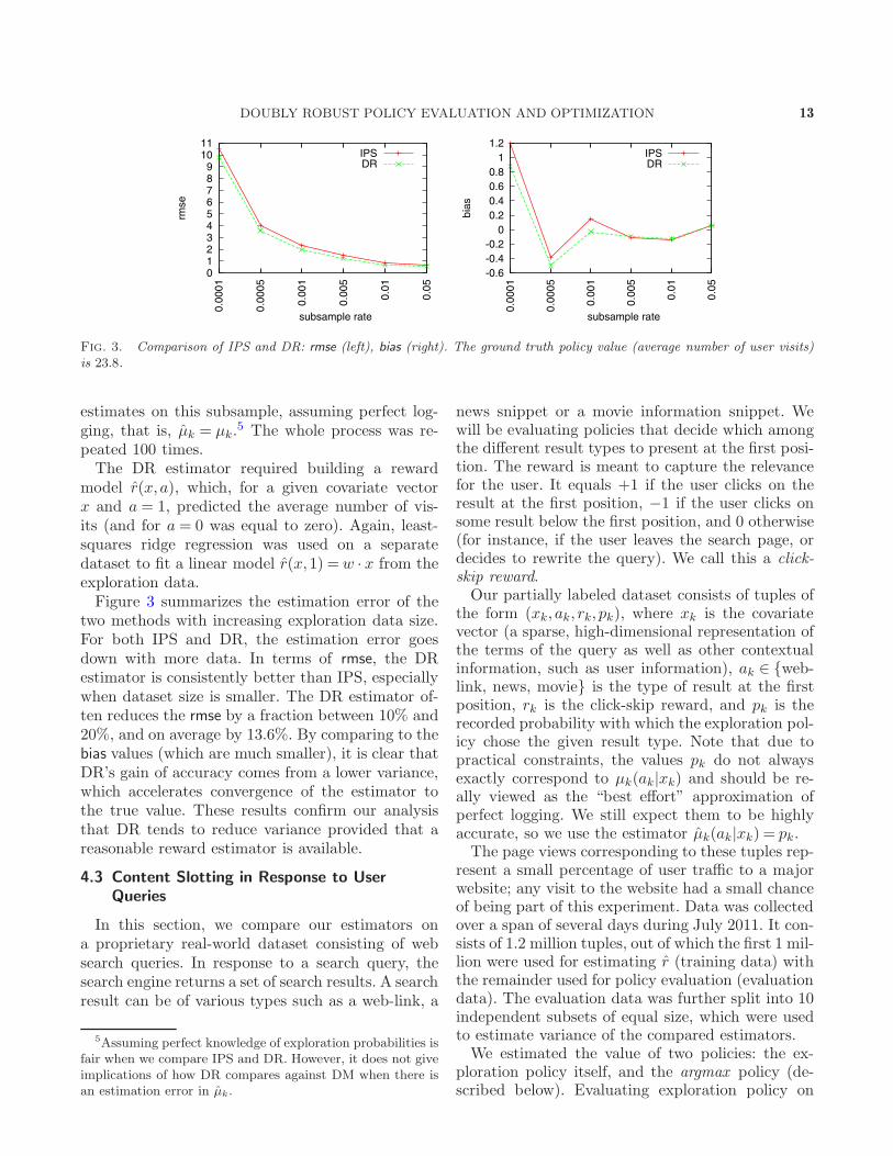
Fig. 3. Comparison of IPS and DR: rmse (left), bias (right). The ground truth policy value (average number of user visits)is 23.8.

estimates on this subsample, assuming perfect log-ging, that is, µk = µk.

5 The whole process was re-peated 100 times.The DR estimator required building a reward

model r(x,a), which, for a given covariate vectorx and a = 1, predicted the average number of vis-its (and for a = 0 was equal to zero). Again, least-squares ridge regression was used on a separatedataset to fit a linear model r(x,1) =w · x from theexploration data.Figure 3 summarizes the estimation error of the

two methods with increasing exploration data size.For both IPS and DR, the estimation error goesdown with more data. In terms of rmse, the DRestimator is consistently better than IPS, especiallywhen dataset size is smaller. The DR estimator of-ten reduces the rmse by a fraction between 10% and20%, and on average by 13.6%. By comparing to thebias values (which are much smaller), it is clear thatDR’s gain of accuracy comes from a lower variance,which accelerates convergence of the estimator tothe true value. These results confirm our analysisthat DR tends to reduce variance provided that areasonable reward estimator is available.

4.3 Content Slotting in Response to User

Queries

In this section, we compare our estimators ona proprietary real-world dataset consisting of websearch queries. In response to a search query, thesearch engine returns a set of search results. A searchresult can be of various types such as a web-link, a

5Assuming perfect knowledge of exploration probabilities isfair when we compare IPS and DR. However, it does not giveimplications of how DR compares against DM when there isan estimation error in µk.

news snippet or a movie information snippet. Wewill be evaluating policies that decide which amongthe different result types to present at the first posi-tion. The reward is meant to capture the relevancefor the user. It equals +1 if the user clicks on theresult at the first position, −1 if the user clicks onsome result below the first position, and 0 otherwise(for instance, if the user leaves the search page, ordecides to rewrite the query). We call this a click-skip reward.Our partially labeled dataset consists of tuples of

the form (xk, ak, rk, pk), where xk is the covariatevector (a sparse, high-dimensional representation ofthe terms of the query as well as other contextualinformation, such as user information), ak ∈ {web-link, news, movie} is the type of result at the firstposition, rk is the click-skip reward, and pk is therecorded probability with which the exploration pol-icy chose the given result type. Note that due topractical constraints, the values pk do not alwaysexactly correspond to µk(ak|xk) and should be re-ally viewed as the “best effort” approximation ofperfect logging. We still expect them to be highlyaccurate, so we use the estimator µk(ak|xk) = pk.The page views corresponding to these tuples rep-

resent a small percentage of user traffic to a majorwebsite; any visit to the website had a small chanceof being part of this experiment. Data was collectedover a span of several days during July 2011. It con-sists of 1.2 million tuples, out of which the first 1 mil-lion were used for estimating r (training data) withthe remainder used for policy evaluation (evaluationdata). The evaluation data was further split into 10independent subsets of equal size, which were usedto estimate variance of the compared estimators.We estimated the value of two policies: the ex-

ploration policy itself, and the argmax policy (de-scribed below). Evaluating exploration policy on


Table 2

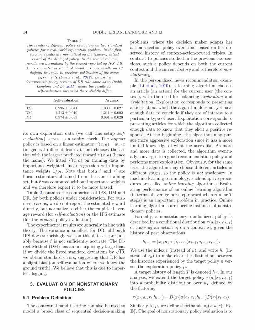
The results of different policy evaluators on two standardpolicies for a real-world exploration problem. In the firstcolumn, results are normalized by the (known) actualreward of the deployed policy. In the second column,

results are normalized by the reward reported by IPS. All± are computed as standard deviations over results on 10

disjoint test sets. In previous publication of the sameexperiments (Dudık et al., 2012), we used a

deterministic-policy version of DR (the same as in Dudık,Langford and Li, 2011), hence the results forself-evaluation presented there slightly differ

Self-evaluation Argmax

IPS 0.995± 0.041 1.000± 0.027DM 1.213± 0.010 1.211± 0.002DR 0.974± 0.039 0.991± 0.026

its own exploration data (we call this setup self-evaluation) serves as a sanity check. The argmaxpolicy is based on a linear estimator r′(x,a) =wa ·x(in general different from r), and chooses the ac-tion with the largest predicted reward r′(x,a) (hencethe name). We fitted r′(x,a) on training data byimportance-weighted linear regression with impor-tance weights 1/pk. Note that both r and r′ arelinear estimators obtained from the same trainingset, but r was computed without importance weightsand we therefore expect it to be more biased.Table 2 contains the comparison of IPS, DM and

DR, for both policies under consideration. For busi-ness reasons, we do not report the estimated rewarddirectly, but normalize to either the empirical aver-age reward (for self-evaluation) or the IPS estimate(for the argmax policy evaluation).The experimental results are generally in line with

theory. The variance is smallest for DR, althoughIPS does surprisingly well on this dataset, presum-ably because r is not sufficiently accurate. The Di-rect Method (DM) has an unsurprisingly large bias.If we divide the listed standard deviations by

√10,

we obtain standard errors, suggesting that DR hasa slight bias (on self-evaluation where we know theground truth). We believe that this is due to imper-fect logging.

5. EVALUATION OF NONSTATIONARY

POLICIES

5.1 Problem Definition

The contextual bandit setting can also be used tomodel a broad class of sequential decision-making

problems, where the decision maker adapts heraction-selection policy over time, based on her ob-served history of context-action-reward triples. Incontrast to policies studied in the previous two sec-tions, such a policy depends on both the currentcontext and the current history and is therefore non-stationary.In the personalized news recommendation exam-

ple (Li et al., 2010), a learning algorithm choosesan article (an action) for the current user (the con-text), with the need for balancing exploration andexploitation. Exploration corresponds to presentingarticles about which the algorithm does not yet haveenough data to conclude if they are of interest to aparticular type of user. Exploitation corresponds topresenting articles for which the algorithm collectedenough data to know that they elicit a positive re-sponse. At the beginning, the algorithm may pur-sue more aggressive exploration since it has a morelimited knowledge of what the users like. As moreand more data is collected, the algorithm eventu-ally converges to a good recommendation policy andperforms more exploitation. Obviously, for the sameuser, the algorithm may choose different articles indifferent stages, so the policy is not stationary. Inmachine learning terminology, such adaptive proce-dures are called online learning algorithms. Evalu-ating performance of an online learning algorithm(in terms of average per-step reward when run for Tsteps) is an important problem in practice. Onlinelearning algorithms are specific instances of nonsta-tionary policies.Formally, a nonstationary randomized policy is

described by a conditional distribution π(at|xt, ht−1)of choosing an action at on a context xt, given thehistory of past observations

ht−1 = (x1, a1, r1), . . . , (xt−1, at−1, rt−1).

We use the index t (instead of k), and write ht (in-stead of zk) to make clear the distinction betweenthe histories experienced by the target policy π ver-sus the exploration policy µ.A target history of length T is denoted hT . In our

analysis, we extend the target policy π(at|xt, ht−1)into a probability distribution over hT defined bythe factoring

π(xt, at, rt|ht−1) =D(xt)π(at|xt, ht−1)D(rt|xt, at).

Similarly to µ, we define shorthands πt(x,a, r), Pπt ,

Eπt . The goal of nonstationary policy evaluation is to


estimate the expected cumulative reward of policyπ after T rounds:

V1:T = EhT∼π

[

T∑

t=1

rt

]

.

In the news recommendation example, rt indicateswhether a user clicked on the recommended article,and V1:T is the expected number of clicks garneredby an online learning algorithm after serving T uservisits. A more effective learning algorithm, by defi-nition, will have a higher V1:T value (Li et al., 2010).Again, to have unbiased policy evaluation, we as-

sume that if πt(a|x) > 0 for any t (and some his-tory ht−1) then µk(a|x)> 0 for all k (and all possi-ble histories zk−1). This clearly holds for instance ifµk(a|x)> 0 for all a.In our analysis of nonstationary policy evaluation,

we assume perfect logging, that is, we assume accessto probabilities

pk := µk(ak|xk).Whereas in general this assumption does not hold, itis realistic in some applications such as those on theInternet. For example, when a website chooses onenews article from a pool to recommend to a user,engineers often have full control/knowledge of howto randomize the article selection process (Li et al.,2010; Li et al., 2011).

5.2 Relation to Dynamic Treatment Regimes

The nonstationary policy evaluation problem de-fined above is closely related to DTR analysis ina longitudinal observational study. Using the samenotation, the inference goal in DTR is to estimatethe expected sum of rewards by following a possiblyrandomized rule π for T steps.6 Unlike contextualbandits, there is no assumption on the distributionfrom which the data zn is generated. More precisely,given an exploration policy µ, the data generationis described by

µ(xk, ak, rk|zk−1)

=D(xk|zk−1)µ(ak|xk, zk−1)D(rk|xk, ak, zk−1).

Compared to the data-generation process in contex-tual bandits (see Section 3.1), one allows the laws

6In DTR often the goal is to estimate the expectation of acomposite outcome that depends on the entire length-T tra-jectory. However, the objective of composite outcomes caneasily be reformulated as a sum of properly redefined rewards.

of xk and rk to depend on history zk−1. The tar-get policy π is subject to the same conditional laws.The setting in longitudinal observational studies istherefore more general than contextual bandits.IPS-style estimators (such as DR of the previous

section) can be extended to handle nonstationarypolicy evaluation, where the likelihood ratios arenow the ratios of likelihoods of the whole length-T trajectories. In DTR analysis, it is often assumedthat the number of trajectories is much larger thanT . Under this assumption and with T small, thevariance of IPS-style estimates is on the order ofO(1/n), diminishing to 0 as n→∞.In contextual bandits, one similarly assumes n≫

T . However, the number of steps T is often large,ranging from hundreds to millions. The likelihoodratio for a length-T trajectory can be exponentialin T , resulting in exponentially large variance. Asa concrete example, consider the case where theexploration policy (i.e., the treatment mechanism)chooses actions uniformly at random from K pos-sibilities, and where the target policy π is a deter-ministic function of the current history and context.The likelihood ratio of any trajectory is exactly KT ,and there are n/T trajectories (by breaking zn inton/T pieces of length T ). Assuming bounded vari-ance of rewards, the variance of IPS-style estimatorsgiven data zn is O(TKT /n), which can be extremelylarge (or even vacuous) for even moderate values ofT , such as those in the studies of online learning inthe Internet applications.In contrast, the “replay” approach of Li et al.

(2011) takes advantage of the independence be-tween (xk, rk) and history zk−1. It has a varianceof O(KT/n), ignoring logarithmic terms, when theexploration policy is uniformly random. When theexploration data is generated by a nonuniformly ran-dom policy, one may apply rejection sampling tosimulate uniformly random exploration, obtaininga subset of the exploration data, which can thenbe used to run the replay approach. However, thismethod may discard a large fraction of data, espe-cially when the historical actions in the log are cho-sen from a highly nonuniform distribution, whichcan yield an unacceptably large variance. The nextsubsection describes an improved replay-based esti-mator that uses doubly-robust estimation as well asa variant of rejection sampling.

5.3 A Nonstationary Policy Evaluator

Our replay-based nonstationary policy evaluator(Algorithm 1) takes advantage of high accuracy


Algorithm 1

DR-ns(π, {(xk, ak, rk, pk)}k=1,2,...,n, r, q, cmax, T )

Input:

target nonstationary policy πexploration data {(xk, ak, rk, pk)}k=1,2,...,n

reward estimator r(x,a)rejection sampling parameters:

q ∈ [0,1] and cmax ∈ (0,1]number of steps T for estimation

Initialize:

simulated history of target policy h0←∅

simulated step of target policy t← 0acceptance rate multiplier c1← cmax

cumulative reward estimate VDR-ns← 0cumulative normalizing weight C← 0importance weights seen so far Q←∅

For k = 1,2, . . . consider event (xk, ak, rk, pk):

(1) Vk← r(xk, πt) +πt(ak |xk)

pk· (rk − r(xk, ak))

(2) VDR-ns← VDR-ns + ctVk

(3) C←C + ct(4) Q←Q ∪ { pk

πt(ak |xk)}

(5) Let uk ∼ uniform[0,1]

(6) If uk ≤ ctπt(ak |xk)pk

(a) ht← ht−1 + (xk, ak, rk)(b) t← t+1(c) if t= T + 1, go to “Exit”(d) ct←min{cmax, qth quantile of Q}

Exit: If t < T + 1, report failure and terminate;otherwise, return:

cumulative reward estimate VDR-nsaverage reward estimate V avg

DR-ns := VDR-ns/C

of DR estimator while tackling nonstationarity viarejection sampling. We substatially improve sam-ple use (i.e., acceptance rate) in rejection samplingwhile only modestly increasing the bias. This algo-rithm is referred to as DR-ns, for “doubly robustnonstationary.” Over the run of the algorithm, weprocess the exploration history and run rejectionsampling [Steps (5)–(6)] to create a simulated his-tory ht of the interaction between the target policyand the environment. If the algorithm manages tosimulate T steps of history, it exits and returns anestimate VDR-ns of the cumulative reward V1:T , andan estimate V avg

DR-ns of the average reward V1:T /T ;

otherwise, it reports failure indicating not enoughdata is available.Since we assume n≫ T , the algorithm fails with

a small probability as long as the exploration pol-icy does not assign too small probabilities to actions.Specifically, let α> 0 be a lower bound on the accep-tance probability in the rejection sampling step; thatis, the condition in Step (6) succeeds with probabil-ity at least α. Then, using the Hoeffding’s inequality,one can show that the probability of failure of thealgorithm is at most δ if

n≥ T + ln(e/δ)

α.

Note that the algorithm returns one “sample” ofthe policy value. In reality, the algorithm continu-ously consumes a stream of n data, outputs a sam-ple of policy value whenever a length-T history issimulated, and finally returns the average of thesesamples. Suppose we aim to simulate m histories oflength T . Again, by Hoeffding’s inequality, the prob-ability of failing to obtain m trajectories is at mostδ if

n≥ mT + ln(e/δ)

α.

Compared with naive rejection sampling, our ap-proach differs in two respects. First, we use not onlythe accepted samples, but also the rejected ones toestimate the expected reward E

πt [r] with a DR esti-

mator [see Step (1)]. As we will see below, the valueof 1/ct is in expectation equal to the total numberof exploration samples used while simulating the tthaction of the target policy. Therefore, in Step (2), weeffectively take an average of 1/ct estimates of Eπ

t [r],decreasing the variance of the final estimator. Thisis in addition to lower variance due to the use of thedoubly robust estimate in Step (1).The second modification is in the control of the

acceptance rate (i.e., the bound α above). Whensimulating the tth action of the target policy,we accept exploration samples with a probabilitymin{1, ctπt/pk} where ct is a multiplier [see Steps(5)–(6)]. We will see below that the bias of the esti-mator is controlled by the probability that ctπt/pkexceeds 1, or equivalently, that pk/πt falls below ct.As a heuristic toward controlling this probability,we maintain a set Q consisting of observed densityratios pk/πt, and at the beginning of simulating thetth action, we set ct to the qth quantile of Q, forsome small value of q [Step (6)(d)], while never al-lowing it to exceed some predetermined cmax. Thus,


the value q approximately corresponds to the prob-ability value that we wish to control. Setting q = 0,we obtain the unbiased case (in the limit). By usinglarger values of q, we increase the bias, but reachthe length T with fewer exploration samples thanksto increased acceptance rate. A similar effect is ob-tained by varying cmax, but the control is cruder,since it ignores the evaluated policy. In our exper-iments, we therefore set cmax = 1 and rely on q tocontrol the acceptance rate. It is an interesting openquestion how to select q and c in practice.To study our algorithm DR-ns, we modify the defi-

nition of the exploration history so as to include thesamples uk from the uniform distribution used bythe algorithm when processing the kth explorationsample. Thus, we have an augmented definition

zk = (x1, a1, r1, u1, . . . , xk, ak, rk, uk).

With this in mind, expressions Pµk and E

µk in-

clude conditioning on variables u1, . . . , uk−1, and µis viewed as a distribution over augmented histo-ries zn.For convenience of analysis, we assume in this sec-

tion that we have access to an infinite explorationhistory z (i.e., zn for n =∞) and that the countert in the pseudocode eventually becomes T + 1 withprobability one (at which point hT is generated).Such an assumption is mild in practice when n ismuch larger than T .Formally, for t ≥ 1, let κ(t) be the index of the

tth sample accepted in Step (6); thus, κ convertsan index in the target history into an index inthe exploration history. We set κ(0) = 0 and defineκ(t) =∞ if fewer than t samples are accepted. Notethat κ is a deterministic function of the history z(thanks to including samples uk in z). We assumethat Pµ[κ(T ) =∞] = 0. This means that the algo-rithm (together with the exploration policy µ) gen-erates a distribution over histories hT ; we denotethis distribution π.Let B(t) = {κ(t− 1)+ 1, κ(t− 1)+ 2, . . . , κ(t)} for

t≥ 1 denote the set of sample indices between the(t−1)st acceptance and the tth acceptance. This setof samples is called the tth block. The contributionof the tth block to the value estimator is denotedVB(t) =

∑

k∈B(t) Vk. After completion of T blocks,the two estimators returned by our algorithm are

VDR-ns =T∑

t=1

ctVB(t), V avgDR-ns =

∑Tt=1 ctVB(t)

∑Tt=1 ct|B(t)|

.

5.4 Bias Analysis

A simple approach to evaluating a nonstationarypolicy is to divide the exploration data into sev-eral parts, run the algorithm separately on eachpart to generate simulated histories, obtaining es-

timates V(1)DR-ns, . . . , V

(m)DR-ns, and return the average

∑mi=1 V

(i)DR-ns/m.7 Here, we assume n is large enough

so that m simulated histories of length T can begenerated with high probability. Using standardconcentration inequalities, we can then show thatthe average is within O(1/

√m) of the expectation

Eµ[VDR-ns]. The remaining piece is then bounding

the bias term Eµ[VDR-ns]−Eπ[∑T

t=1 rt].8

Recall that VDR-ns =∑T

t=1 ctVB(t). The source ofbias are events when ct is not small enough to guar-antee that ctπt(ak|xk)/pk is a probability. In thiscase, the probability that the kth exploration sam-ple includes the action ak and is accepted is

pkmin

{

1,ctπt(ak|xk)

pk

}

=min{pk, ctπt(ak|xk)},(5.1)

which may violate the unbiasedness requirement ofrejection sampling, requiring that the probability ofacceptance be proportional to πt(ak|xk).Conditioned on zk−1 and the induced target his-

tory ht−1, define the event

Ek := {(x,a) : ctπt(a|x)> µk(a|x)},

which contributes to the bias of the estimate, be-cause it corresponds to cases when the minimum inequation (5.1) is attained by pk. Associated with thisevent is the “bias mass” εk, which measures (up toscaling by ct) the difference between the probabilityof the bad event under πt and under the run of ouralgorithm:

εk :=P(x,a)∼πt[Ek]−P(x,a)∼µk

[Ek]/ct.

Notice that from the definition of Ek, this mass isnonnegative. Since the first term is a probability,this mass is at most 1. We will assume that this

7We only consider estimators for cumulative rewards (notaverage rewards) in this section. We assume that the divisioninto parts is done sequentially, so that individual estimates arebuilt from nonoverlapping sequences of T consecutive blocksof examples.

8As shown in Li et al. (2011), when m is constant, makingT large does not necessarily reduce variance of any estimatorof nonstationary policies.


mass is bounded away from 1, that is, that thereexists ε such that for all k and zk−1

0≤ εk ≤ ε < 1.

The following theorem analyzes how much bias isintroduced in the worst case, as a function of ε. Itshows how the bias mass controls the bias of ourestimator.

Theorem 5.1. For T ≥ 1,∣

∣

∣

∣

∣

Eµ

[

T∑

t=1

ctVB(t)

]

−Eπ

[

T∑

t=1

rt

]∣

∣

∣

∣

∣

≤ T (T + 1)

2· ε

1− ε.

Intuitively, this theorem says that if a bias of ε isintroduced in round t, its effect on the sum of re-wards can be felt for T − t rounds. Summing overrounds, we expect to get an O(εT 2) effect on the es-timator of the cumulative reward. In general a veryslight bias can result in a significantly better accep-

tance rate, and hence more replicates V(i)DR-ns.

This theorem is the first of this sort for policy eval-uators, although the mechanics of its proof have ap-peared in model-based reinforcement-learning (e.g.,Kearns and Singh, 1998).To prove the main theorem, we state two technical

lemmas bounding the differences of probabilities andexpectations under the target policy and our algo-rithm (for proofs of lemmas, see Appendix F). Thetheorem follows as their immediate consequence. Re-call that π denotes the distribution over target his-tories generated by our algorithm (together with theexploration policy µ).

Lemma 5.2. Let t ≤ T , k ≥ 1 and let zk−1 besuch that the kth exploration sample marks the be-ginning of the tth block, that is, κ(t−1) = k−1. Letht−1 and ct be the target history and acceptance ratemultiplier induced by zk−1. Then:

∑

x,a

|Pµk [xκ(t) = x,aκ(t) = a]− πt(x,a)| ≤

2ε

1− ε,

|ctEµk [VB(t)]−E

πt [r]| ≤

ε

1− ε.

Lemma 5.3.∑

hT

|π(hT )− π(hT )| ≤ (2εT )/(1− ε).

Proof of Theorem 5.1. First, bound |Eµ[ct ·VB(t)]−Eπ[rt]| using the previous two lemmas, thetriangle inequality and Holder’s inequality:

|Eµ[ctVB(t)]−Eπ[rt]|

= |Eµ[ctEµκ(t)[VB(t)]]−Eπ[rt]|

≤ |Eµ[Eπt [rt]]−Eπ[E

πt [rt]]|+

ε

1− ε

=

∣

∣

∣

∣

Eht−1∼π

[

Eπt

[

r− 1

2

]]

− Eht−1∼π

[

Eπt

[

r− 1

2

]]∣

∣

∣

∣

+ε

1− ε

≤ 1

2

∑

ht−1

|π(ht−1)− π(ht−1)|+ε

1− ε

≤ 1

2· 2ε(t− 1)

1− ε+

ε

1− ε=

εt

1− ε.

The theorem now follows by summing over t andusing the triangle inequality. �

6. EXPERIMENTS: THE NONSTATIONARY

CASE

We now study how DR-ns may achieve greatersample efficiency than rejection sampling throughthe use of a controlled bias. We evaluate our estima-tor on the problem of a multiclass multi-label clas-sification with partial feedback using the publiclyavailable dataset rcv1 (Lewis et al., 2004). In thisdata, the goal is to predict whether a news article isin one of many Reuters categories given the contentsof the article. This dataset is chosen instead of theUCI benchmarks in Section 4 because of its biggersize, which is helpful for simulating online learning(i.e., adaptive policies).

6.1 Data Generation

For multi-label dataset like rcv1, an example hasthe form (x, Y ), where x is the covariate vector andY ⊆ {1, . . . ,K} is the set of correct class labels.9

In our modeling, we assume that any y ∈ Y is thecorrect prediction for x. Similar to Section 4.1, anexample (x, Y ) may be interpreted as a bandit eventwith context x and loss l(Y,a) := I(a /∈ Y ), for ev-ery action a ∈ {1, . . . ,K}. A classifier can be inter-preted as a stationary policy whose expected loss

9The reason why we call the covariate vector x rather thanx becomes in the sequel.


is its classification error. In this section, we againaim at evaluating expected policy loss, which canbe understood as negative reward. For our exper-iments, we only use the K = 4 top-level classes inrcv1, namely {C,E,G,M}. We take a random se-lection of 40,000 data points from the whole datasetand call the resulting dataset D.To construct a partially labeled exploration data-

set, we simulate a stationary but nonuniform explo-ration policy with a bias toward correct answers.This is meant to emulate the typical setting wherea baseline system already has a good understandingof which actions are likely best. For each example(x, Y ), a uniformly random value s(a) ∈ [0.1,1] isassigned independently to each action a, and the fi-nal probability of action a is determined by

µ1(a|x, Y, s) =0.3× s(a)∑

a′ s(a′)

+0.7× I(a ∈ Y )

|Y | .

Note that this policy will assign a nonzero probabil-ity to every action. Formally, our exploration policyis a function of an extended context x = (x, Y, s),and our data generating distribution D(x) includesthe generation of the correct answers Y and valuess. Of course, we will be evaluating policies π thatonly get to see x, but have no access to Y and s.Also, the estimator l (recall that we are evaluatingloss here, not reward) is purely a function of x anda. We stress that in a real-world setting, the explo-ration policy would not have access to all correctanswers Y .

6.2 Evaluation of a Nonstationary Policy

As described before, a fixed (nonadaptive) classi-fier can be interpreted as a stationary policy. Simi-larly, a classifier that adapts as more data arrive isequivalent to a nonstationary policy.In our experiments, we evaluate performance of an

adaptive ǫ-greedy classifier defined as follows: withprobability ǫ = 0.1, it predicts a label drawn uni-formly at random from {1,2, . . . ,K}; with probabil-ity 1 − ǫ, it predicts the best label according to alinear score (the “greedy” label):

argmaxa{wt

a · x},

where {wta}a∈{1,...,K} is a set of K weight vectors

at time t. This design mimics a commonly used ǫ-greedy exploration strategy for contextual bandits(e.g., Li et al., 2010). Weight vectors wt

a are ob-tained by fitting a logistic regression model for the

binary classification problem a ∈ Y (positive) ver-sus a /∈ Y (negative). The data used to fit wt

a is de-scribed below. Thus, the greedy label is the mostlikely label according to the current set of logis-tic regression models. The loss estimator l(x, a) isalso obtained by fitting a logistic regression modelfor a ∈ Y versus a /∈ Y , potentially on a differentdataset.We partition the whole data D randomly into

three disjoint subsets: Dinit (initialization set),Dvalid (validation set), and Deval (evaluation set),consisting of 1%, 19%, and 80% of D, respectively.Our goal in this experiment is to estimate the ex-pected loss, V1:T , of an adaptive policy π afterT = 300 rounds.The full-feedback set Dinit is used to fit the loss

estimator l.Since Dvalid is a random subset of D, it may be

used to simulate the behavior of policy π to obtainan unbiased estimate of V1:T . We do this by takingan average of 2000 simulations of π on random shuf-fles of the set Dvalid. This estimate, denoted V1:T , isa highly accurate approximation to (the unknown)V1:T , and serves as our ground truth.To assess different policy-value estimators, we ran-

domly permute Deval and transform it into a par-tially labeled set as described in Section 6.1. On theresulting partially labeled data, we then evaluate thepolicy π up to round T , obtaining an estimate ofV1:T . If the exploration history is not exhausted, westart the evaluation of π again, continuing with thenext exploration sample, but restarting from emptytarget history (for T rounds), and repeat until weuse up all the exploration data. The final estimateis the average across thus obtained replicates. We re-peat this process (permutation of Deval, generationof exploration history, and policy evaluation untilusing up all exploration data) 50 times, so that wecan compare the 50 estimates against the groundtruth V1:T to compute bias and standard deviationof a policy-value estimator.Finally, we describe in more detail the ε-greedy

adaptive classifier π being evaluated:

• First, the policy is initialized by fitting weights w0a

on the full-feedback set Dinit (similarly to l). Thisstep mimics the practical situation where one usu-ally has prior information (in the form of eitherdomain knowledge or historical data) to initializea policy, instead of starting from scratch.


• After this “warm-start” step, the “online” phasebegins: in each round, the policy observes a ran-domly selected x, predicts a label in an ǫ-greedyfashion (as described above), and then observesthe corresponding 0/1 prediction loss. The policyis updated every 15 rounds. On those rounds, weretrain weights wt

a for each action a, using the fullfeedback set Dinit as well as all the data from theonline phase where the policy chose action a. Theonline phase terminates after T = 300 rounds.

6.3 Compared Evaluators

We compared the following evaluators describedearlier: DM for direct method, RS for the unbiasedevaluator based on rejection sampling and “replay”(Li et al., 2011), and DR-ns as in Algorithm 1 (withcmax = 1). We also tested a variant of DR-ns, whichdoes not monitor the quantile, but instead uses ctequal to minD µ1(a|x); we call it DR-ns-wc since ituses the worst-case (most conservative) value of ctthat ensures unbiasedness of rejection sampling.

6.4 Results

Table 3 summarizes the accuracy of different eval-uators in terms of rmse (root mean squared error),bias (the absolute difference between the average es-timate and the ground truth) and stdev (standarddeviation of the estimates across different runs). Itshould be noted that, given the relatively small num-ber of trials, the measurement of bias is not statis-tically significant. However, the table provides 95%confidence interval for the rmse metric that allows ameaningful comparison.It is clear that although rejection sampling is guar-

anteed to be unbiased, its variance is usually thedominating part of its rmse. At the other extreme isthe direct method, which has the smallest variancebut often suffers large bias. In contrast, our methodDR-ns is able to find a good balance between the two

Table 3

Nonstationary policy evaluation results

Evaluator rmse (±95% C.I.) bias stdev

DM 0.0329± 0.0007 0.0328 0.0027RS 0.0179± 0.0050 0.0007 0.0181DR-ns-wc 0.0156± 0.0037 0.0086 0.0132DR-ns (q = 0) 0.0129± 0.0034 0.0046 0.0122DR-ns (q = 0.01) 0.0089± 0.0017 0.0065 0.0062DR-ns (q = 0.05) 0.0123± 0.0017 0.0107 0.0061DR-ns (q = 0.1) 0.0946± 0.0015 0.0946 0.0053

extremes and, with proper selection of the param-eter q, is able to make the evaluation results muchmore accurate than others.It is also clear that the main benefit of DR-ns is its

low variance, which stems from the adaptive choiceof ct values. By slightly violating the unbiasednessguarantee, it increases the effective data size signifi-cantly, hence reducing the variance of its evaluation.For q > 0, DR-ns was able to extract many more tra-jectories of length 300 for evaluating π, while RS andDR-ns-wc were able to find only one such trajectoryout of the evaluation set. In fact, if we increase thetrajectory length of π from 300 to 500, both RS andDR-ns-wc are not able to construct a complete tra-jectory of length 500 and fail the task completely.

7. CONCLUSIONS

Doubly robust policy estimation is an effectivetechnique which virtually always improves on thewidely used inverse propensity score method. Ouranalysis shows that doubly robust methods tendto give more reliable and accurate estimates, forevaluating both stationary and nonstationary poli-cies. The theory is corroborated by experiments onbenchmark data as well as two large-scale real-worldproblems. In the future, we expect the DR techniqueto become common practice in improving contextualbandit algorithms.

APPENDIX A: PROOFS OF LEMMAS 3.1–3.3

Throughout proofs in this appendix, we write rand r∗ instead of r(x,a) and r∗(x,a) when x and aare clear from the context, and similarly for ∆ andk.

Lemma 3.1. The range of Vk is bounded as

|Vk| ≤ 1 +M.

Proof.

|Vk|=∣

∣

∣

∣

r(xk, ν) +ν(ak|xk)µk(ak|xk)

· (rk − r(xk, ak))

∣

∣

∣

∣

≤ |r(xk, ν)|+ν(ak|xk)µk(ak|xk)

· |rk − r(xk, ak)|

≤ 1 +M,

where the last inequality follows because r and rkare bounded in [0,1]. �

Lemma 3.2. The expectation of the term Vk is

Eµk [Vk] = E

(x,a)∼ν[r∗(x,a) + (1− k(x,a))∆(x,a)].


Proof.

Eµk [Vk] = E

(x,a,r)∼µk

[

r(x, ν) +ν(a|x)µk(a|x)

· k · (r− r)

]

= Ex∼D

[r(x, ν)]

+ Ex∼D

[

∑

a∈A

µk(a|x) Er∼D( · |x,a)

[

ν(a|x)µk(a|x)

· k · (r− r)

]]

= Ex∼D

[r(x, ν)]

+ Ex∼D

[

∑

a∈A

ν(a|x) Er∼D( · |x,a)

[k · (r− r)]

]

= E(x,a)∼ν

[r] + E(x,a,r)∼ν

[k · (r− r)]

= E(x,a)∼ν

[r∗ + (r− r∗) + k · (r∗ − r)](A.1)

= E(x,a)∼ν

[r∗ + (1− k)∆].�

Lemma 3.3. The variance of the term Vk can bedecomposed and bounded as follows:

Vµk [Vk](i)

= Vx∼D

[ Ea∼ν( · |x)

[r∗(x,a)

+ (1− k(x,a))∆(x,a)]]

− Ex∼D

[ Ea∼ν( · |x)

[k(x,a)∆(x,a)]2]

+ E(x,a)∼ν

[

ν(a|x)µk(a|x)

· k(x,a) · Vr∼D( · |x,a)

[r]

]

+ E(x,a)∼ν

[

ν(a|x)µk(a|x)

· k(x,a)∆(x,a)2]

.

Vµk [Vk](ii)

≤ Vx∼D

[r∗(x, ν)]

+ 2 E(x,a)∼ν

[|(1− k(x,a))∆(x,a)|]

+M E(x,a)∼ν

[k(x,a)

· Er∼D( · |x,a)

[(r− r(x,a))2]].

Proof.

Eµk [V

2k ] = E

(x,a,r)∼µk

[(

r(x, ν) +ν(a|x)µk(a|x)

· k

· (r− r)

)2]

= Ex∼D

[r(x, ν)2]

+ 2 E(x,a,r)∼µk

[

r(x, ν)

· ν(a|x)µk(a|x)

· k · (r− r)

]

+ E(x,a,r)∼µk

[

ν(a|x)µk(a|x)

· ν(a|x)µk(a|x)

· k · (r− r)2]

= Ex∼D

[r(x, ν)2](A.2)

+ 2 E(x,a,r)∼ν

[r(x, ν) · k · (r− r)]

+ E(x,a,r)∼ν

[

ν(a|x)µk(a|x)

· k · (r− r)2]

= E(x,a)∼ν

[(r(x, ν)− k∆)2](A.3)

− E(x,a)∼ν

[2k∆2] +E,

where E denotes the term

E := E(x,a,r)∼ν

[

ν(a|x)µk(a|x)

· k · (r− r)2]

.

To obtain an expression for the variance of Vk, firstnote that by equation (A.1),

Eµk [Vk] = E

(x,a)∼ν[r(x, ν)− k∆].(A.4)

Combining this with equation (A.3), we obtain

Vµk [Vk] = V

(x,a)∼ν[r(x, ν)− k∆]

− E(x,a)∼ν

[2k∆2] +E

= Vx∼D

[ Ea∼ν( · |x)

[r(x, ν)− k∆]]

+ Ex∼D

[ Va∼ν( · |x)

[r(x, ν)− k∆]]

− Ex∼D

[ Va∼ν( · |x)

[k∆]]

− Ex∼D

[ Ea∼ν( · |x)

[k∆]2] +E

= Vx∼D

[ Ea∼ν( · |x)

[r∗ + (1− k)∆]]


+ Ex∼D

[ Va∼ν( · |x)

[k∆]]

− Ex∼D

[ Va∼ν( · |x)

[k∆]]

− Ex∼D

[ Ea∼ν( · |x)

[k∆]2] +E

= Vx∼D

[ Ea∼ν( · |x)

[r∗ + (1− k)∆]]

− Ex∼D

[ Ea∼ν( · |x)

[k∆]2] +E.

We now obtain part (i) of the lemma by decompos-ing the term E:

E = E(x,a,r)∼ν

[

ν(a|x)µk(a|x)

· k · (r− r∗)2]

+ E(x,a)∼ν

[

ν(a|x)µk(a|x)

· k · (r∗ − r)2]

= E(x,a)∼ν

[

ν(a|x)µk(a|x)

· k · Vr∼D( · |x,a)

[r]

]

+ E(x,a)∼ν

[

ν(a|x)µk(a|x)

· k∆2

]

.

To prove part (ii) of the lemma, first note that

r(x, ν)2 = (r∗(x, ν) + Ea∼ν( · |x)

[∆(x,a)])2

= r∗(x, ν)2 +2r∗(x, ν) Ea∼ν( · |x)

[∆(x,a)]

+ Ea∼ν( · |x)

[∆(x,a)]2

= r∗(x, ν)2 +2r(x, ν) Ea∼ν( · |x)

[∆(x,a)]

− Ea∼ν( · |x)

[∆(x,a)]2

≤ r∗(x, ν)2 +2r(x, ν) Ea∼ν( · |x)

[∆(x,a)].

Plugging this in equation (A.2), we obtain

Eµk [V

2k ] = E

x∼D[r(x, ν)2]

+ 2 E(x,a,r)∼ν

[r(x, ν) · k · (r− r)] +E

≤ Ex∼D

[r∗(x, ν)2]

+ 2 Ex∼D

[r(x, ν) Ea∼ν( · |x)

[∆]]

+ 2 E(x,a)∼ν

[r(x, ν) · (−k) ·∆]+E

= Ex∼D

[r∗(x, ν)2](A.5)

+ 2 E(x,a)∼ν

[r(x, ν) · (1− k) ·∆]+E.

On the other hand, equation (A.4) can be rewrittenas

Eµk [Vk] = E

(x,a)∼ν[r∗(x, ν) + (1− k)∆].

Combining with equation (A.5), we obtain

Vµk [Vk]≤ V

x∼D[r∗(x, ν)]

+ 2 E(x,a)∼ν

[r(x, ν) · (1− k)∆]

− 2 Ex∼D

[r∗(x, ν)] E(x,a)∼ν

[(1− k)∆]

− E(x,a)∼ν

[(1− k)∆]2 +E

≤ Vx∼D

[r∗(x, ν)]

+ 2 E(x,a)∼ν

[(r(x, ν)− 12)(1− k)∆]

− 2 Ex∼D

[r∗(x, ν)− 12 ] E

(x,a)∼ν[(1− k)∆]

+E

≤ Vx∼D

[r∗(x, ν)] + E(x,a)∼ν

[|(1− k)∆|]

+ | E(x,a)∼ν

[(1− k)∆]|+E,

where the last inequality follows by Holder’s inequal-ity and the observations that |r − 1/2| ≤ 1/2 and|r∗− 1/2| ≤ 1/2. Part (ii) now follows by the bound

E = E(x,a,r)∼ν

[

ν(a|x)µk(a|x)

· k · (r− r)2]

≤M E(x,a)∼ν

[k Er∼D( · |x,a)

[(r− r)2]].�

APPENDIX B: FREEDMAN’S INEQUALITY

The following is a corollary of Theorem 1 ofBeygelzimer et al. (2011). It can be viewed as aversion of Freedman’s inequality Freedman’s (1975).Let y1, . . . , yn be a sequence of real-valued randomvariables. Let Ek denote E[ · |y1, . . . , yk−1] and Vk

conditional variance.

Theorem B.1. Let V,D ∈R such that

n∑

k=1

Vk[yk]≤ V,


and for all k, |yk−Ek[yk]| ≤D. Then for any δ > 0,with probability at least 1− δ,∣

∣

∣

∣

∣

n∑

k=1

yk−n∑

k=1

Ek[yk]

∣

∣

∣

∣

∣

≤ 2max{D ln(2/δ),√

V ln(2/δ)}.

APPENDIX C: IMPROVED FINITE-SAMPLEERROR BOUND

In this appendix, we analyze the error of VDR inestimating the value of a stationary policy ν. Wegeneralize the analysis of Section 3.4.3 by replacingconditions on the ranges of variables by conditionson the moments.For a function f :X ×A→ R and 1 ≤ p <∞, we

define the Lp(ν) norm as usual:

‖f‖p,ν =E(x,a)∼ν [|f(x,a)|p]1/p.For p=∞, ‖f‖∞,ν is the essential supremum of |f |under ν.As in Section 3.4.3, we first simplify Lemmas 3.1–

3.3, and then apply Freedman’s inequality to obtaina specific error bound.

Lemma C.1. Let 1 ≤ p, q ≤ ∞ be such that1/p + 1/q = 1. Assume there are finite constantsM,er, δ∆, δ, max ≥ 0 such that with probability oneunder µ, for all k:

ν(ak|xk)/µk(ak|xk)≤M,

‖∆‖q,ν ≤ δ∆,

‖1− k‖p,ν ≤ δ,

‖k‖p,ν ≤ max,

E(x,a)∼ν

[ Er∼D( · |x,a)

[(r(x,a)− r)2]q]1/q ≤ er.

Then with probability one under µ, for all k:

|Eµk [Vk]− V | ≤ δδ∆,

Vµk [Vk]≤Vx∼D[r

∗(x, ν)] + 2δδ∆ +Mmaxer.

Proof. The bias and variance bound followfrom Lemma 3.2 and Lemma 3.3(ii), respectively,by Holder’s inequality. �

Theorem C.2. If assumptions of Lemma C.1hold, then with probability at least 1− δ,

|VDR − V |≤ δδ∆

+ 2max

{

(1 +M) ln(2/δ)

n,

√

(Vx∼D[r∗(x, ν)] + 2δδ∆ +Mmaxer) ln(2/δ)

n

}

.


random variables Vk, whose range and variance arebounded using Lemma 3.1 and C.1. �

APPENDIX D: DIRECT LOSS MINIMIZATION

Given cost-sensitive multiclass classification data{(x, l1, . . . , lK)}, we perform approximate gradi-ent descent on the policy loss (or classificationerror). In the experiments of Section 4.1, pol-icy ν is specified by K weight vectors θ1, . . . , θK .Given x ∈ X , the policy predicts as follows: ν(x) =argmaxa∈{1,...,K}{x · θa}.To optimize θa, we adapt the “toward-better”

version of the direct loss minimization method ofMcAllester, Hazan and Keshet (2011) as follows:given any data point (x, l1, . . . , lK) and the currentweights θa, the weights are adjusted by

θa1 ← θa1 + ηx,

θa2 ← θa2 − ηx,

where a1 = argmaxa{x · θa − ǫla}, a2 = argmaxa{x ·θa}, η ∈ (0,1) is a decaying learning rate, and ǫ > 0is an input parameter.For computational reasons, we actually perform

batch updates rather than incremental updates. Up-dates continue until the weights converge. We foundthat the learning rate η = t−0.3/2, where t is thebatch iteration, worked well across all datasets. Theparameter ǫ was fixed to 0.1 for all datasets.Furthermore, since the policy loss is not convex

in the weight vectors, we repeat the algorithm 20times with randomly perturbed starting weights andthen return the best run’s weight according to thelearned policy’s loss in the training data. We alsotried using a holdout validation set for choosing thebest weights out of the 20 candidates, but did notobserve benefits from doing so.

APPENDIX E: FILTER TREE

The Filter Tree (Beygelzimer, Langford and Ravi-kumar, 2008) is a reduction from multiclass cost-sensitive classification to binary classification. Itsinput is of the same form as for Direct Loss Min-imization, but its output is a Filter Tree: a decisiontree, where each inner node is itself implementedby some binary classifier (called base classifier), andleaves correspond to classes of the original multi-class problem. As base classifiers we used J48 de-cision trees implemented in Weka 3.6.4 (Hall et al.,


2009). Thus, there are 2-class decision trees in thenodes, with the nodes arranged as per a Filter Tree.Training in a Filter Tree proceeds bottom-up, butthe classification in a trained Filter Tree proceedsroot-to-leaf, with the running time logarithmic inthe number of classes. We did not test the all-pairsFilter Tree, which classifies examples in the time lin-ear in the number of classes, similar to DLM.

APPENDIX F: PROOFS OF LEMMAS 5.2

AND 5.3

Lemma 5.2. Let t ≤ T , k ≥ 1 and let zk−1 besuch that the kth exploration sample marks the be-ginning of the tth block, that is, κ(t−1) = k−1. Letht−1 and ct be the target history and acceptance ratemultiplier induced by zk−1. Then:

∑

x,a

|Pµk [xκ(t) = x,aκ(t) = a]− πt(x,a)|(F.1)

≤ 2ε

1− ε,

|ctEµk [VB(t)]−E

πt [r]| ≤

ε

1− ε.(F.2)

Proof. We begin by showing equation (F.1).Consider the mth exploration sample (x,a) ∼ µm

and assume that this sample is in the tth block. Theprobability of accepting this sample is

Pu∼µm( · |x,a)

[

u≤ ctπt(a|x)µm(a|x)

]

= I[(x,a) ∈ Em] +ctπt(a|x)µm(a|x) I[(x,a) /∈ Em],

where I[ · ] is the indicator function equal to 1 whenits argument is true and 0 otherwise. The probabilityof seeing and accepting a sample (x,a) from µm is

acceptm(x,a)

:= µm(x,a)

(

I[(x,a) ∈ Em]

+ctπt(a|x)µm(a|x) I[(x,a) /∈ Em]

)

= µm(x,a)I[(x,a) ∈ Em]

+ ctπt(x,a)I[(x,a) /∈ Em]

= ctπt(x,a)

− (ctπt(x,a)− µm(x,a))I[(x,a) ∈ Em]

and the marginal probability of accepting a samplefrom µm is

acceptm(∗) :=∑

x,a

acceptm(x,a)

= ct − ctεm = ct(1− εm).

In order to accept the mth exploration sample, sam-ples k through m− 1 must be rejected. The proba-bility of eventually accepting (x,a), conditioned onzk−1 is therefore

Pµk(xκ(t) = x,aκ(t) = a)

=Eµk

[

∞∑

m≥k

acceptm(x,a)

m−1∏

k′=k

(1− acceptk′(∗))]

= ctπt(x,a)(F.3)

·Eµk

[

∞∑

m≥k

m−1∏

k′=k


−Eµk

[

∞∑

m≥k

(ctπt(x,a)− µm(x,a))(F.4)

· I[(x,a) ∈ Em]

·m−1∏

k′=k


.

To bound |Pµk [xκ(t) = x,aκ(t) = a] − πt(x,a)| and

prove equation (F.1), we first need to bound equa-tions (F.3) and (F.4). Note that from the definitionof Em, the expression inside the expectation of equa-tion (F.4) is always nonnegative. Let E1(x,a) denotethe expression in equation (F.3) and E2(x,a) the ex-pression in equation (F.4). We bound E1(x,a) andE2(x,a) separately, using bounds 0≤ εm ≤ ε:

E1(x,a) = ctπt(x,a)Eµk

[

∞∑

m≥k

m−1∏

k′=k


≤ ctπt(x,a)Eµk

[

∞∑

m≥k

m−1∏

k′=k

(1− ct(1− ε))

]

=πt(x,a)

1− ε,

E1(x,a)≥ ctπt(x,a)Eµk

[

∞∑

m≥k

m−1∏

k′=k

(1− ct)

]

= πt(x,a),


E2(x,a) =Eµk

[

∞∑

m≥k

(ctπt(x,a)− µm(x,a))

· I[(x,a) ∈ Em]

·m−1∏

k′=k


≤Eµk

[

∞∑

m≥k


· I[(x,a) ∈ Em]

· (1− ct(1− ε))m−k

]

.

Now we are ready to prove equation (F.1):

∑

x,a

|Pµk [xκ(t) = x,aκ(t) = a]− πt(x,a)|

=∑

x,a

|E1(x,a)− πt(x,a)−E2(x,a)|

≤∑

x,a

|E1(x,a)− πt(x,a)|+∑

x,a

E2(x,a)

≤∑

x,a

πt(x,a)ε

1− ε

+Eµk

[

∞∑

m≥k

∑

x,a


· I[(x,a) ∈ Em](1− ct(1− ε))m−k

]

=ε

1− ε+E

µk

[

∞∑

m≥k

ctεm(1− ct(1− ε))m−k

]

≤ 2ε

1− ε

proving equation (F.1).Let reachm denote the indicator of the event that

the mth sample is in block t (i.e., samples k, k +1, . . . ,m− 1 are rejected). Then

Eµk [VB(t)] =

∞∑

m=k

Eµk [Vm reachm]

=∞∑

m=k

Eµk [E

µm[Vm reachm]]

=

∞∑

m=k

Eµk [reachmE

µm[Vm]],(F.5)

where equation (F.5) follows because the event ofreaching the mth sample depends only on the pre-ceding samples, and hence it is a deterministic func-tion of zm−1. Plugging Lemma 3.2 in equation (F.5),we obtain

ctEµk [VB(t)]

= ct Er∼πt

[r]

∞∑

m=k

Eµk [reachm]

= ct Er∼πt

[r]Eµk

[

∞∑

m=k

m−1∏

k′=k


(because Er∼πt[r] is a deterministic function of

zk−1). This can be bounded, similarly as before, as

Er∼πt

[r]≤ ctEµk [VB(t)]≤

Er∼πt[r]

1− ε

yielding equation (F.2). �

Lemma 5.3.∑

hT

|π(hT )− π(hT )| ≤ (2εT )/(1− ε).

Proof. We prove the lemma by induction andthe triangle inequality (essentially following Kakade,Kearns and Langford, 2003). The lemma holds forT = 0 since there is only one empty history (andhence both π and π are point distributions over h0).Now assume the lemma holds for T − 1. We proveit for T :

∑

hT

|π(hT )− π(hT )|

=∑

hT−1

∑

(xT ,aT ,rT )

|π(hT−1)πT (xT , aT , rT )

− π(hT−1)πT (xT , aT , rT )|

≤∑

hT−1

∑

(xT ,aT ,rT )

(|π(hT−1)πT (xT , aT , rT )

− π(hT−1)πT (xT , aT , rT )|+ |π(hT−1)πT (xT , aT , rT )

− π(hT−1)πT (xT , aT , rT )|)

= EhT−1∼π

[

∑

(xT ,aT ,rT )

|πT (xT , aT , rT )


− πT (xT , aT , rT )|]

+∑

hT−1

|π(hT−1)− π(hT−1)|

≤ 2ε

1− ε+

2ε(T − 1)

1− ε=

2εT

1− ε.

�

APPENDIX G: PROGRESSIVE VALIDATION

POLICY

In Section 4.1.3, we showed how the stationary DRestimator can be used not only for policy evaluation,but also for policy optimization by transforming thecontextual bandit problem into a cost sensitive clas-sification problem.In this appendix, we show how the nonstation-

ary DR estimator, when applied to an online learn-ing algorithm, can also be used to obtain a high-performing stationary policy. The value of this pol-icy concentrates around the average per-step re-ward estimated for the online learning algorithm.Thus, to the extent that the online algorithmachieves a high reward, so does this stationarypolicy. The policy is constructed using the ideasbehind the “progressive validation” error bound(Blum, Kalai and Langford, 1999), and hence wecall it a “progressive validation policy.”Assume that the algorithm DR-ns successfully ter-

minates after generating T blocks. The progressivevalidation policy is the randomized stationary policyπPV defined as

πPV(a|x) :=T∑

t=1

ct|B(t)|C

π(a|x,ht−1).

Conceptually, this policy first picks among the histo-ries h0, . . . , hT−1 with probabilities c1|B(1)|/C, . . . ,ct|B(T )|/C, and then executes the policy π giventhe chosen history. We extend πPV to a distributionover triples

πPV(x,a, r) =D(x)πPV(a|x)D(r|x,a).We will show that the average reward estimator

V avgDR-ns returned by our algorithm estimates the ex-

pected reward of πPV with an error O(1/√N) where

N is the number of exploration samples used to gen-erate T blocks. Thus, assuming that the nonstation-ary policy π improves with more data, we expectto obtain the best-performing progressive validationpolicy with themost accurate value estimate by run-ning the algorithm DR-ns on all of the explorationdata.

The error bound in the theorem below is proved byanalyzing range and variance of Vk using Lemma 3.8.The theorem relies on the following conditions (mir-roring the assumptions of Lemma 3.8):

• There is a constant M > 0 such that πt(ak|xk)/pk ≤M .

• There is a constant er > 0 such that

E(x,a)∼πt[ED[(r− r)2 | x,a]]≤ er.

• There is a constant vr > 0 such that

Vx∼D[Er,a∼πt( ·,· |x)[r]]≤ vr.

These conditions ensure boundedness of density ra-tios, squared prediction error of rewards, and vari-ance of a conditional expected reward, respectively.It should be noted that, since rewards are assumedto be in [0,1], one can always choose er and vr thatare no greater than 1.

Theorem G.1. Let N be the number of explo-ration samples used to generate T blocks, that is,N =

∑Tt=1 |B(t)|. Assume the above conditions hold

for all k and t (and all histories zk−1 and ht−1).Then, with probability at least 1− δ,

|V avgDR-ns − E

r∼πPV

[r]|

≤ Ncmax

C

· 2max

{

(1 +M) ln(2/δ)

N,

√

(vr +Mer) ln(2/δ)

N

}

.


random variables ctVk, whose range and variancecan be bounded using Lemma 3.8 and the boundct ≤ cmax. In applying Lemma 3.8, note that δ = 0and max = 1, because µk = µk. �

ACKNOWLEDGMENTS

We thank the editors and reviewers for their vastamount of patience and efforts that have improvedthe paper substantially.

REFERENCES

Agarwal, D., Chen, B.-C., Elango, P. and Ramakrish-

nan, R. (2013). Content recommendation on web portals.Comm. ACM 56 92–101.


Asuncion, A. and Newman, D. J. (2007). UCI machinelearning repository. Available at http://www.ics.uci.

edu/~mlearn/MLRepository.html.Auer, P., Cesa-Bianchi, N., Freund, Y. and

Schapire, R. E. (2002/03). The nonstochastic mul-tiarmed bandit problem. SIAM J. Comput. 32 48–77(electronic). MR1954855

Barto, A. G. and Anandan, P. (1985). Pattern-recognizingstochastic learning automata. IEEE Trans. Systems ManCybernet. 15 360–375. MR0793841

Beygelzimer, A. and Langford, J. (2009). The offset treefor learning with partial labels. In ACM SIGKDD Con-ference on Knowledge Discovery and Data Mining (KDD)129–138. Association for Computing Machinery, New York.

Beygelzimer, A., Langford, J. and Ravikumar, P.

(2008). Multiclass classification with filter-trees. Unpub-lished technical report. Available at http://arxiv.org/

abs/0902.3176.Beygelzimer, A., Langford, J., Li, L., Reyzin, L. and

Schapire, R. E. (2011). Contextual bandit algorithmswith supervised learning guarantees. In International Con-ference on Artificial Intelligence and Statistics (AI&Stats)19–26. jmlr.org.

Blum, A., Kalai, A. and Langford, J. (1999). Beatingthe hold-out: Bounds for K-fold and progressive cross-validation. In Proceedings of the Twelfth Annual Confer-ence on Computational Learning Theory (Santa Cruz, CA,1999) 203–208. ACM, New York. MR1811616

Bottou, L., Peters, J., Quinonero-Candela, J.,Charles, D. X., Chickering, D. M., Portugaly, E.,Ray, D., Simard, P. and Snelson, E. (2013). Counter-factual reasoning and learning systems: The example ofcomputational advertising. J. Mach. Learn. Res. 14 3207–3260. MR3144461

Cassel, C. M., Sarndal, C. E. and Wretman, J. H.

(1976). Some results on generalized difference estimationand generalized regression estimation for finite popula-tions. Biometrika 63 615–620. MR0445666

Chan, D., Ge, R., Gershony, O., Hesterberg, T. andLambert, D. (2010). Evaluating online ad campaigns in apipeline: Causal models at scale. In ACM SIGKDD Con-ference on Knowledge Discovery and Data Mining (KDD)7–16. ACM, New York.

Chapelle, O. and Li, L. (2012). An empirical evaluation ofThompson sampling. In Advances in Neural InformationProcessing Systems 24 (NIPS) 2249–2257. Curran Asso-ciates, Red Hook, NY.

Dudık, M., Langford, J. and Li, L. (2011). Doubly robustpolicy evaluation and learning. In International Conferenceon Machine Learning (ICML).

Dudık, M., Erhan, D., Langford, J. and Li, L. (2012).Sample-efficient nonstationary-policy evaluation for con-textual bandits. In Conference on Uncertainty in ArtificialIntelligence (UAI) 1097–1104. Association for ComputingMachinery, New York.

Freedman, D. A. (1975). On tail probabilities for martin-gales. Ann. Probab. 3 100–118. MR0380971

Gretton, A., Smola, A. J., Huang, J., Schmittfull, M.,Borgwardt, K. and Scholkopf, B. (2008). Dataset shift

in machine learning. In Covariate Shift and Local Learn-ing by Distribution Matching (J. Quinonero-Candela,M. Sugiyama, A. Schwaighofer and N. Lawrence,eds.) 131–160. MIT Press, Cambridge, MA.

Hall, M., Frank, E., Holmes, G., Pfahringer, B.,Reutemann, P. and Witten, I. H. (2009). The WEKAdata mining software: An update. SIGKDD Explorations11 10–18.

Hazan, E. and Kale, S. (2009). Better algorithms for benignbandits. In Proceedings of the Twentieth Annual ACM-SIAM Symposium on Discrete Algorithms 38–47. SIAM,Philadelphia, PA. MR2809303

Horvitz, D. G. and Thompson, D. J. (1952). A general-ization of sampling without replacement from a finite uni-verse. J. Amer. Statist. Assoc. 47 663–685. MR0053460

Kakade, S., Kearns, M. and Langford, J. (2003). Explo-ration in metric state spaces. In International Conferenceon Machine Learning (ICML) 306–312. AAAI Press, PaloAlto, CA.

Kang, J. D. Y. and Schafer, J. L. (2007). Demystifyingdouble robustness: A comparison of alternative strategiesfor estimating a population mean from incomplete data.Statist. Sci. 22 523–539. MR2420458

Kearns, M. and Singh, S. (1998). Near-optimal reinforce-ment learning in polynomial time. In International Confer-ence on Machine Learning (ICML) 260–268. Morgan Kauf-mann, Burlington, MA.

Lambert, D. and Pregibon, D. (2007). More bang for theirbucks: Assessing new features for online advertisers. In In-ternational Workshop on Data Mining for Online Advertis-ing and Internet Economy (ADKDD) 100–107. Associationfor Computing Machinery, New York.

Langford, J., Strehl, A. L. and Wortman, J. (2008). Ex-ploration scavenging. In International Conference on Ma-chine Learning (ICML) 528–535. Association for Comput-ing Machinery, New York, NY.

Langford, J. and Zhang, T. (2008). The Epoch–Greedy al-gorithm for contextual multi-armed bandits. In Advancesin Neural Information Processing Systems (NIPS) 817–824. Curran Associates, Red Hook, NY.

Lewis, D. D., Yang, Y., Rose, T. G. and Li, F. (2004).RCV1: A new benchmark collection for text categorizationresearch. J. Mach. Learn. Res. 5 361–397.

Li, L., Chu, W., Langford, J. and Schapire, R. E. (2010).A contextual-bandit approach to personalized news arti-cle recommendation. In International Conference on WorldWide Web (WWW) 661–670. Association for ComputingMachinery, New York.

Li, L., Chu, W., Langford, J. and Wang, X. (2011). Un-biased offline evaluation of contextual-bandit-based newsarticle recommendation algorithms. In ACM InternationalConference on Web Search and Data Mining (WSDM)297–306. Association for Computing Machinery, New York.

Lunceford, J. K. and Davidian, M. (2004). Stratificationand weighting via the propensity score in estimation ofcausal treatment effects: A comparative study. Stat. Med.23 2937–2960.

McAllester, D., Hazan, T. and Keshet, J. (2011). Directloss minimization for structured prediction. In Advances in

http://www.ics.uci.edu/~mlearn/MLRepository.html

http://www.ics.uci.edu/~mlearn/MLRepository.html

http://www.ams.org/mathscinet-getitem?mr=1954855


http://arxiv.org/abs/0902.3176

http://arxiv.org/abs/0902.3176

http://jmlr.org









Neural Information Processing Systems (NIPS) 1594–1602.

Curran Associates, Red Hook, NY.

Murphy, S. A. (2003). Optimal dynamic treatment regimes.

J. R. Stat. Soc. Ser. B Stat. Methodol. 65 331–366.

MR1983752

Murphy, S. A., van der Laan, M. J. and Robins, J. M.

(2001). Marginal mean models for dynamic regimes. J.

Amer. Statist. Assoc. 96 1410–1423. MR1946586

Orellana, L., Rotnitzky, A. and Robins, J. M. (2010).

Dynamic regime marginal structural mean models for es-

timation of optimal dynamic treatment regimes. Part I:

Main content. Int. J. Biostat. 6 Art. 8, 49. MR2602551

Precup, D., Sutton, R. S. and Singh, S. P. (2000). El-

igibility traces for off-policy evaluation. In International

Conference on Machine Learning (ICML) 759–766. Mor-

gan Kaufmann, Burlington, MA.

Robbins, H. (1952). Some aspects of the sequential design

of experiments. Bull. Amer. Math. Soc. (N.S.) 58 527–535.

MR0050246

Robins, J. (1986). A new approach to causal inference

in mortality studies with a sustained exposure period—

Application to control of the healthy worker survivor effect.

Mathematical models in medicine: Diseases and epidemics.

Part 2. Math. Modelling 7 1393–1512. MR0877758

Robins, J. M. (1998). Marginal structural models. In 1997

Proceedings of the American Statistical Association, Sec-

tion on Bayesian Statistical Science 1–10. Amer. Statist.Assoc., Alexandria, VA.

Robins, J. M. and Rotnitzky, A. (1995). Semiparametricefficiency in multivariate regression models with missingdata. J. Amer. Statist. Assoc. 90 122–129. MR1325119

Robins, J. M., Rotnitzky, A. and Zhao, L. P. (1994).Estimation of regression coefficients when some regressorsare not always observed. J. Amer. Statist. Assoc. 89 846–866. MR1294730

Rotnitzky, A. and Robins, J. M. (1995). Semiparametricregression estimation in the presence of dependent censor-ing. Biometrika 82 805–820. MR1380816

Shimodaira, H. (2000). Improving predictive inference un-der covariate shift by weighting the log-likelihood function.J. Statist. Plann. Inference 90 227–244. MR1795598

Strehl, A., Langford, J., Li, L. and Kakade, S. (2011).Learning from logged implicit exploration data. In Ad-vances in Neural Information Processing Systems (NIPS)2217–2225. Curran Associates, Red Hook, NY.

Vansteelandt, S., Bekaert, M. and Claeskens, G.

(2012). On model selection and model misspecificationin causal inference. Stat. Methods Med. Res. 21 7–30.MR2867536

Zhang, B., Tsiatis, A. A., Laber, E. B. and Davidian, M.

(2012). A robust method for estimating optimal treatmentregimes. Biometrics 68 1010–1018. MR3040007












Doubly Robust Policy Evaluation and Optimization

Documents

Transcript of Doubly Robust Policy Evaluation and Optimization