Optimization and Analysis of Doubly-Curved Kirigami Space ...
128
Optimization and Analysis of Doubly-Curved Kirigami Space Frames by Michael Ramirez B.S. in Civil and Environmental Engineering The University of Texas at Austin, 2019 Submitted to the Department of Civil and Environmental Engineering in Partial Fulfillment of the Requirements for the degree of MASTER OF ENGINEERING IN CIVIL AND ENVIRONMENTAL ENGINEERING at the MASSACHUSETTS INSTITUTE OF TECHNOLOGY May 2020 ©2020 Michael R. Ramirez. All rights reserved. The author hereby grants to MIT permission to reproduce and to distribute publicly paper and electronic copies of this thesis document in whole or in part in any medium now known or hereafter created. Signature of Author: Michael Ramirez Department of Civil and Environmental Engineering May 8, 2020 Certified by: Gordana Herning Lecturer in Civil and Environmental Engineering Thesis Supervisor Accepted by: Colette L. Heald Professor of Civil and Environmental Engineering Chair, Graduate Program Committee
Transcript of Optimization and Analysis of Doubly-Curved Kirigami Space ...

Optimization and Analysis of Doubly-Curved
Kirigami Space Frames by
Michael Ramirez
B.S. in Civil and Environmental Engineering
The University of Texas at Austin, 2019
Submitted to the Department of Civil and Environmental Engineering
in Partial Fulfillment of the Requirements for the degree of
MASTER OF ENGINEERING IN CIVIL AND ENVIRONMENTAL ENGINEERING
at the
MASSACHUSETTS INSTITUTE OF TECHNOLOGY
May 2020
©2020 Michael R. Ramirez. All rights reserved.
The author hereby grants to MIT permission to reproduce and to distribute publicly paper and electronic
copies of this thesis document in whole or in part in any medium now known or hereafter created.
Signature of Author:
Michael Ramirez
Department of Civil and Environmental Engineering
May 8, 2020
Certified by:
Gordana Herning
Lecturer in Civil and Environmental Engineering
Thesis Supervisor
Accepted by:
Colette L. Heald
Professor of Civil and Environmental Engineering
Chair, Graduate Program Committee

2

3
Optimization and Analysis of Doubly-Curved
Kirigami Space Frames
by
Michael Ramirez
Submitted to the Department of Civil and Environmental Engineering
on May 8, 2020 in Partial Fulfillment of the Requirements for the
Degree of Master of Engineering in Civil and Environment Engineering
Abstract
Inspired by the Japanese art of origami and kirigami, the concept of Spin-Valence is used to
transform a two-dimensional sheet of metal into a three-dimensional spatial frame. Previous
iterations of this design were developed by Emily Baker of the University of Arkansas, mainly by
making scaled models. Recently a frame assembly of Spin-Valence units was analyzed
experimentally and computationally to characterize the structural behavior of the system.
Transitioning from flat to curved systems and building a full-scale pavilion motivates this study.
This thesis focuses on using optimization to computationally construct doubly-curved
configurations of the Spin-Valence pattern logic from input surfaces. To accomplish this,
optimization in Rhinoceros v6 and Python v3.7 is used to create a coherent primary and secondary
surface. The final structure is then subjected to finite element analysis using Abaqus 2017.
Throughout history, spanning structures have evolved from linear elements such as beams to
arches and finally to spatial systems. Each iteration manipulates form to counterbalance internal
element forces with better material efficiency and architectural flexibility. Doubly-curved Spin-
Valence surfaces are developed to allow greater versatility of form and frame characteristics.
Thesis Supervisor: Gordana Herning
Title: Lecturer in Civil and Environmental Engineering

4
5
Acknowledgements
I place my deepest gratitude for my thesis advisor, Dr. Gordana Herning, who has convincingly
guided and encouraged me even when the road became tough. Without her persistent help, the goal
of this project would not have been realized.
For Emily Baker and Edmund Harriss from the University of Arkansas and Nick Sherrow-Groves
from Arup, I would like to recognize the invaluable assistance and mentorship that you have given
me. Becoming part of the Spin-Valence team has been one of the most fruitful experiences of my
academic career.
I am indebted to the Massachusetts Institute of Technology’s Department of Civil and
Environmental Engineering for giving me the opportunity to explore structural engineering in a
new light and supporting me through the journey.
I would like to thank all my schoolmates and friends from MIT for making this year an
unforgettable experience, especially, Camp Seats, Yijiang Huang, and Mohamed Ismail, who
helped with the early configurations of the Spin-Valence deployment algorithm.
Finally, I would like to pay special regards to my lifelong friends and my family, my parents,
Rolando and Paz; my sister, Elaine; and my brother, Matthew. Your loving and continued support
has kept me going this past year.

6
THIS PAGE INTENTIONALLY LEFT BLANK

7
Contents
Abstract ......................................................................................................................................3
Acknowledgements .....................................................................................................................5
Contents .....................................................................................................................................7
List of Figures .......................................................................................................................... 11
List of Tables ............................................................................................................................ 13
1. Introduction.......................................................................................................................... 15
1.1. Characterizing the Spin-Valence Pattern-Logic ................................................................ 15
1.2. Qualitative Modifications to the RES ................................................................................. 17
1.3. Past Work ........................................................................................................................... 18 1.3.1. Structural Analysis by MIT and Arup ............................................................................................. 18 1.3.2. Doubly-Curved Variants of Spin-Valence ...................................................................................... 19
1.4. Motivation ........................................................................................................................... 19
1.5. Thesis Objectives: Computational Formulation and Analysis .......................................... 20
2. Spatial and Deployable Structures ....................................................................................... 21
2.1. Spatial Structures ............................................................................................................... 21
2.2. Deployable Structures ........................................................................................................ 23 2.2.1. Application of Deployable Structures ............................................................................................. 23 2.2.2. Classification of Deployable Structures .......................................................................................... 24
3. Previous Analyses of Kirigami Space Frames ...................................................................... 27
3.1. Motivation ........................................................................................................................... 27
3.2. Preliminary Structural Modifications by Baker ................................................................ 28
3.3. Initial Structural Characterization of the Spin-Valence Frame ........................................ 29 3.3.1. Strain Hardening of Nodal Components ......................................................................................... 29 3.3.2. Self-contact Between System Elements .......................................................................................... 30 3.3.3. Local Buckling Failure at Primary and Secondary Surfaces ............................................................ 30
3.4. Structural Recommendations ............................................................................................. 31
CONTENTS
8
4. Preliminary Computational Modeling for Deployment ........................................................ 33
4.1. Modeling Software .............................................................................................................. 33
4.2. Motivation ........................................................................................................................... 33
4.3. Base Unit Deployment Logic .............................................................................................. 34 4.3.1. Constraints to the Problem ............................................................................................................. 35 4.3.2. Three-Dimensional Configuration-Space ........................................................................................ 35
4.4. Algorithm Limitations and Transition ............................................................................... 38
5. Mathematic Definition for Spin-Valence Geometry Deployment ......................................... 39
5.1. Motivation ........................................................................................................................... 39
5.2. New Base Unit Deployment Logic ...................................................................................... 40 5.2.1. Notation ........................................................................................................................................ 40 5.2.2. Mathematic Constraints ................................................................................................................. 41 5.2.3. Solving the Deployment Equation for Parameters ........................................................................... 41
5.2.3.1: Case 1 (θ = 0): .......................................................................................................................... 46 5.2.3.2: Cases 2 and 3 (𝑡. 𝑟1 = 0) or (𝑡. 𝑟2 = 0) ...................................................................................... 46
6. Algorithms for Computational Primary and Secondary Surface Generation ....................... 49
6.1. Modeling Software .............................................................................................................. 49
6.2. Motivation ........................................................................................................................... 50
6.3. Proposed Workflow for Constructing a Doubly-Curved Pavilion ................................... 50 6.3.1. User-generated surfaces ................................................................................................................. 51 6.3.2. Grasshopper-Produced Secondary Surface ..................................................................................... 52 6.3.3. Optimized Deployed Primary Surface ............................................................................................ 54 6.3.4. Final Meshed Model in Rhino ........................................................................................................ 54 6.3.5. Finite Element Analysis ................................................................................................................. 55
6.4. Computationally Produced Secondary Surface ................................................................. 56 6.4.1. Constraints .................................................................................................................................... 57 6.4.2. Transition to Python-produced Primary Surface ............................................................................. 58
6.5. Optimized Deployment of Primary Surface ....................................................................... 59 6.5.1. Imported Python libraries ............................................................................................................... 59 6.5.2. Notation ........................................................................................................................................ 59 6.5.3. Parameters ..................................................................................................................................... 61 6.5.4. Optimization.................................................................................................................................. 61 6.5.5. File_read ....................................................................................................................................... 62 6.5.6. Objective ....................................................................................................................................... 63 6.5.7. Kirigami ........................................................................................................................................ 63 6.5.8. Distance ........................................................................................................................................ 68 6.5.9. Plot ............................................................................................................................................... 75 6.5.10. Results ............................................................................................................................................. 75
6.5.10.1. Nelder-Mead ............................................................................................................................ 76 6.5.10.2. Powell ...................................................................................................................................... 77 6.5.10.3. TNC (Truncated Newton Conjugate-Gradient) .......................................................................... 79 6.5.10.4. SLSQP (Sequential Least Squares Programming) ...................................................................... 80

CONTENTS
9
6.5.10.5. Summary of 3x14 Assembly Optimization Case Study .............................................................. 82 6.5.10.6. Final Pavilion ........................................................................................................................... 82
6.5.11. Improvements for the Future ............................................................................................................ 84
7. Finite Element Analysis of Proposed Pavilion Design ......................................................... 85
8. Conclusion ........................................................................................................................... 87
8.1. Summary of Contributions ................................................................................................. 87
8.2. Future Work ....................................................................................................................... 88
8.3. Concluding Remarks and Potential Impacts ..................................................................... 89
9. References ............................................................................................................................ 91
Appendix A: Individual Deployment Logic in Mathematica .................................................... 93
Appendix B: Sample Calculation of Deployment in Mathematica ........................................... 99
Appendix C: Computational Primary Surface Python Script ................................................. 105
Objective ........................................................................................................................................ 106
File_Read ....................................................................................................................................... 109
Kirigami......................................................................................................................................... 110
Distance ......................................................................................................................................... 114
Plot ................................................................................................................................................. 118
Appendix D: Additional Images from Chapter 6 Results ....................................................... 121
3x14 Assembly ............................................................................................................................... 122
Nelder-Mead Optimization ........................................................................................................... 123
Powell Optimization ...................................................................................................................... 123
TNC Optimization ......................................................................................................................... 124
SLSQP Optimization ..................................................................................................................... 125
Non-Optimized Pavilion ................................................................................................................ 126
TNC Optimized Pavilion ............................................................................................................... 127
SLSQP Optimized Pavilion ........................................................................................................... 128

CONTENTS
10
THIS PAGE INTENTIONALLY LEFT BLANK

11
List of Figures
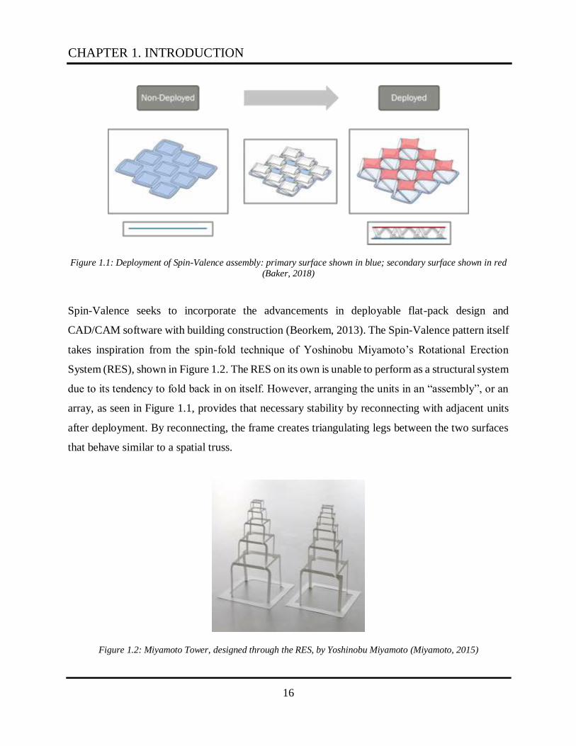
Figure 1.1: Deployment of Spin-Valence assembly: primary surface shown in blue;
secondary surface shown in red (Baker, 2018) ........................................................ 16
Figure 1.2: Miyamoto Tower, designed via the RES, by Yoshinobu Miyamoto
(Miyamoto, 2015) .................................................................................................... 16
Figure 1.3: Pythagorean tiling techniques for unit arrangement in CNC sheet
(Baker and Harriss, n.d.) .......................................................................................... 17
Figure 1.4: Individual structural unit modifications (Baker, 2018) ............................................. 18
Figure 1.5: NPPUs to create spherical double-curved surfaces (Baker and Harriss, n.d.) ............ 19
Figure 1.6: Aesthetic displays of Spin-Valence on University of Arkansas campus
(Baker, 2018) ........................................................................................................... 19
Figure 2.1: Crystal Palace roof spatial frame geometry (Addis, 2006) ....................................... 22
Figure 2.2: Spatial structures examples – San Francisco International Airport (left),
Singapore Jewel Changi airport (middle), Munich Olympiastadion (right)
(SOM, 2000; Saiidi, 2019; Rawn, 2019) .................................................................. 22
Figure 2.3: Origami mobile bridge (left), Rapid deployable military tent (right)
(Hiroshima University, 2015) (Eureka, 2014) .......................................................... 24
Figure 2.4: Deployable structures classification examples (Hanaor and Levy, 2001) ................. 25
Figure 3.1: Baker’s modifications to the initial RES pattern (Baker, 2018) ................................ 28
Figure 3.2: Strain hardening at kirigami unit nodes (Sherrow-Groves and Baker, 2019) ............ 29
Figure 3.3: Contact between angle-legs and primary surface
(Sherrow-Groves and Baker, 2019) .......................................................................... 30
Figure 3.4: Primary surface buckling failure (Sahuc et al., 2019) ............................................... 31
Figure 4.1: Parallel plane units (PPUs) vs. non-parallel plane units (NPPUs) ............................. 34
Figure 4.2: Center line equivalent length pairings for Spin-Valence geometry ........................... 35
Figure 4.3: Assigning S1 through parameters ϴ and ϕ ................................................................ 36
Figure 4.4: Assigning S2 from parameter, τ ............................................................................... 36
Figure 4.5: Locating S4 from intersection of three spheres (left); locating S3 from planar
relationships (right) ................................................................................................. 37
Figure 5.1: Notation for deployment algorithm .......................................................................... 40
Figure 5.2: Rodrigues Rotation Formula notation (Dale, 2015) .................................................. 45
Figure 5.3: Notation for r1 and r2 axes (left); Non-deployed tilting along r1 axis (middle);
tilting along r2 axis (right) ....................................................................................... 46
Figure 6.1: Input curves for surface generation .......................................................................... 51
Figure 6.2: Formulated surface from input curves...................................................................... 52

LIST OF FIGURES
12
Figure 6.3: Boundary conditions for input surface (highlighted in blue)..................................... 52
Figure 6.4: Grid-pattern of secondary surface ............................................................................ 53
Figure 6.5: Optimized Pythagorean tiling of secondary surface ................................................. 53
Figure 6.6: Optimized primary surface ...................................................................................... 54
Figure 6.7: Point connections in the primary surface created by E. Baker .................................. 55
Figure 6.8: Preliminary meshing of primary and secondary surface created by E. Baker (left) ... 55
Figure 6.9: Rendering of the proposed pavilion created by E. Baker (right) .............................. 55
Figure 6.10: Abaqus finite element model of 3x3 assembly ....................................................... 56
Figure 6.11: Secondary surface generated from input surface .................................................... 57
Figure 6.12: Global tiling specifications .................................................................................... 58
Figure 6.13: Labeled primary and secondary vertices ................................................................ 60
Figure 6.14: Offset center-line geometry ................................................................................... 61
Figure 6.15: Orient matrix numbering notation .......................................................................... 68
Figure 6.16: Notation for assigning sides to columns in xn matrix ............................................. 69
Figure 6.17: Sample orient (left) and xn (right) matrices for a 4x4 assembly ............................. 70
Figure 6.18: Flowchart for finding adjacent units ...................................................................... 71
Figure 6.19: pA and pB combinations including segment boundary conditions .......................... 74
Figure 6.20: Plot example using Axis3d .................................................................................... 75
Figure 6.21: Sample 3x14 assembly for optimization analysis ................................................... 76
Figure 6.22: Nelder-Mead optimization results .......................................................................... 77
Figure 6.23: Powell optimization results .................................................................................... 78
Figure 6.24: Steepest descent (blue) vs. Newton method (black) for locating local minima........ 79
Figure 6.25: TNC 1: Theta [.301,.800], Phi [.001,.5] (left), TNC 2: Theta [.301,.900],
Phi [.001,.6] (middle), TNC 3: Theta [.401,.900], Phi [.001,.5] (right) .................. 80
Figure 6.26: SLSQP 1: Theta [.301,.800], Phi [.001,.5] (left), SLSQP 2: Theta [.301,.900],
Phi [.001,.6] (middle), SLSQP 3: Theta [.401,.900], Phi [.001,.5] (right) .............. 81
Figure 6.27: Pavilion design prior to optimization ..................................................................... 82
Figure 6.28: TNC optimization for proposed pavilion design..................................................... 83
Figure 6.29: SLSQP optimization for proposed pavilion design ................................................. 83
Figure 7.1: 3x3 unit assembly for detailed finite element analysis ............................................. 86

13
List of Tables
Table 1: Sphere specifications to locate S4................................................................................. 37
Table 2: Simplified legend for Figure 6.16 ................................................................................ 69
Table 3: Xn matrix rules ............................................................................................................ 70
Table 4: Nelder-Mead Optimization Results .............................................................................. 77
Table 5: Powell Optimization Results........................................................................................ 78
Table 6: TNC Optimization Results........................................................................................... 80
Table 7: SLSQP Optimization Results ....................................................................................... 81
Table 8: Summary of 3x14 Assembly Optimization Results ...................................................... 82
Table 9: Proposed Pavilion Optimization Results ...................................................................... 83

LIST OF TABLES
14
THIS PAGE INTENTIONALLY LEFT BLANK

15
Chapter 1
Introduction
This thesis presents new work in the computational design of doubly-curved kirigami space
frames, expanding upon previous research on deployable structures by Emily Baker (Baker,
2014, 2018). This chapter introduces the topic of Spin-Valence, past work on the subject, and
key applications for a computationally generated Spin-Valence frame from input surfaces.
1.1. Characterizing the Spin-Valence Pattern-Logic
Spin-Valence is a kirigami (cut and fold) pattern-logic that creates a deployable structural system
using a single sheet of CNC plasma cut steel, folded and reconnected to itself, to develop a double-
layer space frame (Baker, 2014, 2018). The system is devised to expand from the thickness of a
single sheet to dual surfaces (primary and secondary), that are connected with continuous
triangulated legs. Figure 1.1 depicts its deployment from a two-dimensional (2D) sheet to a three-
dimensional (3D) spatial frame.
16
Figure 1.1: Deployment of Spin-Valence assembly: primary surface shown in blue; secondary surface shown in red
(Baker, 2018)
Spin-Valence seeks to incorporate the advancements in deployable flat-pack design and
CAD/CAM software with building construction (Beorkem, 2013). The Spin-Valence pattern itself
takes inspiration from the spin-fold technique of Yoshinobu Miyamoto’s Rotational Erection
System (RES), shown in Figure 1.2. The RES on its own is unable to perform as a structural system
due to its tendency to fold back in on itself. However, arranging the units in an “assembly”, or an
array, as seen in Figure 1.1, provides that necessary stability by reconnecting with adjacent units
after deployment. By reconnecting, the frame creates triangulating legs between the two surfaces
that behave similar to a spatial truss.
Figure 1.2: Miyamoto Tower, designed through the RES, by Yoshinobu Miyamoto (Miyamoto, 2015)
CHAPTER 1. INTRODUCTION
17
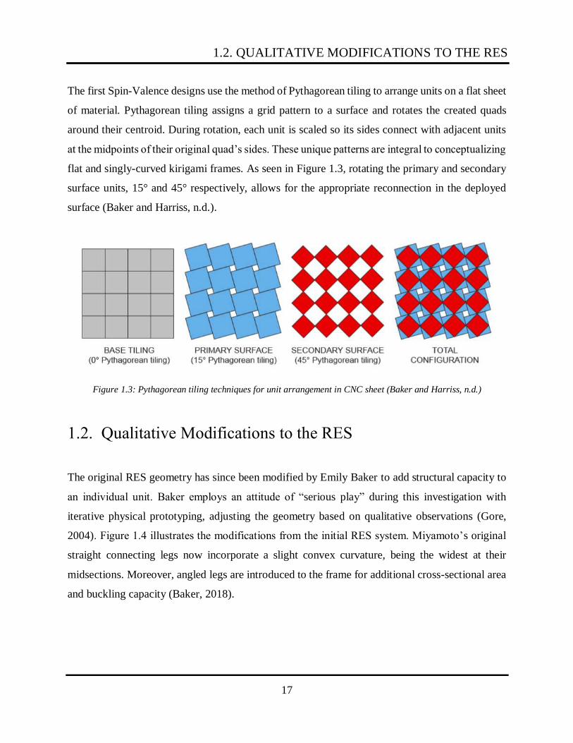
The first Spin-Valence designs use the method of Pythagorean tiling to arrange units on a flat sheet
of material. Pythagorean tiling assigns a grid pattern to a surface and rotates the created quads
around their centroid. During rotation, each unit is scaled so its sides connect with adjacent units
at the midpoints of their original quad’s sides. These unique patterns are integral to conceptualizing
flat and singly-curved kirigami frames. As seen in Figure 1.3, rotating the primary and secondary
surface units, 15° and 45° respectively, allows for the appropriate reconnection in the deployed
surface (Baker and Harriss, n.d.).
Figure 1.3: Pythagorean tiling techniques for unit arrangement in CNC sheet (Baker and Harriss, n.d.)
1.2. Qualitative Modifications to the RES
The original RES geometry has since been modified by Emily Baker to add structural capacity to
an individual unit. Baker employs an attitude of “serious play” during this investigation with
iterative physical prototyping, adjusting the geometry based on qualitative observations (Gore,
2004). Figure 1.4 illustrates the modifications from the initial RES system. Miyamoto’s original
straight connecting legs now incorporate a slight convex curvature, being the widest at their
midsections. Moreover, angled legs are introduced to the frame for additional cross-sectional area
and buckling capacity (Baker, 2018).
1.2. QUALITATIVE MODIFICATIONS TO THE RES

18
Figure 1.4: Individual structural unit modifications (Baker, 2018)
1.3. Past Work
1.3.1. Structural Analysis by MIT and Arup
During the International Association for Shell and Spatial Structures (IASS) Annual Symposium
in 2019, Baker established a team of engineers from MIT and Arup to start initial structural
computational analysis for the Spin-Valence system. This collaboration led to physical testing of
a single kirigami unit and of a 3x3 assembly, coupled with a finite element model created in LS-
DYNA (LSTC, 1978) that was validated using the experimental testing results. Both approaches
explored the structural limitations of the spatial frame in terms of strength, stiffness, ductility, and
buckling, and proposed improvements to the design (Sherrow-Groves and Baker, 2019; Sahuc et
al. 2019)
CHAPTER 1. INTRODUCTION

19
1.3.2. Doubly-Curved Variants of Spin-Valence
To explore possible configurations of Spin-Valence, double-curved variants have been produced,
making use of non-parallel plane units (NPPUs) as seen in Figure 1.5. However, these
arrangements are limited to geometric aggregation instead of user-input surfaces (Baker and
Harriss, n.d.). The next steps for the Spin-Valence system explore creating doubly-curved kirigami
frames that would allow additional geometric configurations.
Figure 1.5: NPPUs to create spherical doubly-curved surfaces (Baker and Harriss, n.d.)
1.4. Motivation
With increased architectural variability and structural capacity, the Spin-Valence system has the
potential to be extended to wider applications including structural installations.
Figure 1.6: Aesthetic displays of Spin-Valence on University of Arkansas campus (Baker, 2018)
1.4. MOTIVATION

20
Extension to various input surfaces would allow Spin-Valence to handle multiple boundary
conditions and loading scenarios. This would yield opportunities for use as long-spanning spatial
structures for temporary bridges, curved vaults, or gabled frames. In addition, its deployable flat-
pack design gives the system enhanced utility for transportation and eliminates the need for
complex assembly of discrete members.
These characteristics differentiate the Spin-Valence frames amongst the established deployable
methods, such as scissor mechanisms. Introducing computational programming to the kirigami
frames can further strengthen the value of the system by highlighting its adaptability.
1.5. Thesis Objectives: Computational Formulation
and Analysis
To produce a workflow for generating variable kirigami frames, a team including Emily Baker, an
architect from the University of Arkansas, Edmund Harriss, a mathematician from the University
of Arkansas, Nick Sherrow-Groves, a structural engineer from Arup, Gordana Herning, a lecturer
at MIT, and the author was formed. Each member contributes their strengths, with Baker and
Harriss focusing on computational geometry and Sherrow-Groves, Herning, and Ramirez
exploring the structural analysis, while still engaging in interdisciplinary conversation. To begin,
a preliminary algorithm for mapping input surfaces has been created, using Rhinoceros v6
(McNeel, 1980) and the Pythagorean tiling method referenced in Section 1.1. Baker and Harriss
progressed the design by producing a computationally formed secondary surface with the Rhino
plug-in, Grasshopper (McNeel, 2007).
This thesis focuses on improving Baker and Harriss’s initial algorithm and creating a script that
mathematically formulates a primary surface from the data obtained for the secondary surface.
Moreover, this paper will investigate the formation of an efficient workflow from input surface
conception to finite element analysis of a completed doubly-curved kirigami frame.
CHAPTER 1. INTRODUCTION

21
Chapter 2
Spatial and Deployable Structures
This chapter discusses a brief literature review of spatial and deployable structures. First, their
features and applications are characterized, and then their respective categorizations are listed.
Deployable structures are a subcategory of spatial structures. The kirigami spatial frame is a new
methodology for deployable structures that takes inspiration from spatial structure precedents.
2.1. Spatial Structures
Prior to the 19th century, horizontal spanning structures, composed of interconnected flat planes,
were the preferred methods for roof and bridge construction. However, deficiencies with out-of-
plane stiffness and stability limit their applications, both structurally and aesthetically. Spatial
structures improve upon these limitations by incorporating three-dimensionality to their restraints
and internal networks of members (Lin and Huang, 2016). The roof structure of London's Crystal
Palace shown in Figure 2.1 is an early example of spatial frame development. Joseph Paxton, the
architect, through prefabrication, efficient geometric force transfers, and pre-tensioning,
significantly reduced construction time and material costs with his design (Addis, 2006). Projects
similar to Paxton’s increased the renown of spatial structures for both their elegant appearance and
economic value.

22
Figure 2.1: Crystal Palace roof spatial frame geometry (Addis, 2006)
Spatial structures can be divided into three categories: spatial truss/grid structures, spatial latticed
shell, and membrane. Figure 2.2 provides an example of each system from left to right. Each
category exploits introducing three-dimensionality to the system in different ways for additional
structural capacity.
Figure 2.2: Spatial structures examples – San Francisco International Airport (left),
Singapore Jewel Changi Airport (middle), Munich Olympiastadion (right)
(SOM, 2000; Saiidi, 2019; Rawn, 2019)
The traditional kirigami frame, once fully deployed, is modeled after the spatial truss system. This
structural method incorporates out-of-plane connections to the traditional planar truss design. 3D
connections establish efficient force transfers, where members are arranged to mutually support
one another against in-plane and out-of-plane loading (Lin and Huang, 2016). The triangulating
legs of the kirigami frame enable these productive force transfers.
CHAPTER 2. SPATIAL AND DEPLOYABLE STRUCTURES
23
Introducing double-curvature to the Spin-Valence design rewards the benefits from latticed shell
structures. Latticed shell structures are composed of a geometric array of singly or doubly-curved
members that interconnect to generate a rigid shell framework (Lin and Huang, 2016).
Throughout history spanning structures have evolved from linear elements such as beams and
columns to arches and finally to spatial systems. Each iteration showcased new ways of
counterbalancing internal element forces and bending moments with higher material efficiency
and greater architecturally variability. Doubly-curved Spin-Valence frames attempts to innovate
the previously flat configuration. Introducing curvature provides greater material performance,
capability for longer spans, and visually appealing designs.
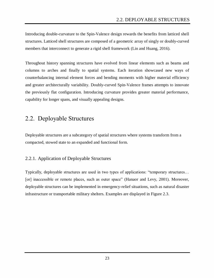
2.2. Deployable Structures
Deployable structures are a subcategory of spatial structures where systems transform from a
compacted, stowed state to an expanded and functional form.
2.2.1. Application of Deployable Structures
Typically, deployable structures are used in two types of applications: “temporary structures…
[or] inaccessible or remote places, such as outer space” (Hanaor and Levy, 2001). Moreover,
deployable structures can be implemented in emergency-relief situations, such as natural disaster
infrastructure or transportable military shelters. Examples are displayed in Figure 2.3.
2.2. DEPLOYABLE STRUCTURES

24
Figure 2.3: Origami mobile bridge (left), Rapid deployable military tent (right)
(Hiroshima University, 2015) (Eureka, 2014)
The kirigami space frame has the potential to satisfy both applications. Baker’s flat pack design
enables the system to have all structural components inscribed computationally into a sheet of
material. This facilitates easier transportation and implementation to areas with little resources.
Currently, reconnection in the deployed surface requires tack-welding for stability, making it
irreversible. However, Baker is exploring other methods such as bolting to make the system more
adaptable to potential construction constraints.
2.2.2. Classification of Deployable Structures
Deployable structures can be classified under two tiers: morphology and kinematics. Morphology
of these systems can either be skeletal (lattice, scissor mechanism), continuous (surface or stressed-
skin), or a hybrid of the two. Kinematics refers to the method of deployment, whether it is driven
by rigid linkages or deformables (cables or fabrics) (Hanaor and Levy, 2001). Figure 2.4 visually
explains both tiers with examples.
CHAPTER 2. SPATIAL AND DEPLOYABLE STRUCTURES

25
Figure 2.4: Deployable structures classification examples (Hanaor and Levy, 2001)
2.2. DEPLOYABLE STRUCTURES

26
THIS PAGE INTENTIONALLY LEFT BLANK
CHAPTER 2. SPATIAL AND DEPLOYABLE STRUCTURES
27
Chapter 3
Previous Analyses of Kirigami Space Frames
This chapter summarizes prior analysis of the Spin-Valence kirigami space frames. These include
qualitative analyses through creating and refining the physical models of various configurations
for the frame (Baker, 2014, 2018), computational form finding (Baker and Harriss, n.d.), and
characterization of structural behavior of frame elements and assemblies (Sherrow-Groves and
Baker, 2019; Sahuc et al., 2019).
3.1. Motivation
As mentioned in Section 1.2, the previous iterations of Spin-Valence units were created through
physical prototyping and qualitative observations of their structural characteristics by Baker.
Creating a computational model for the kirigami frame is an important next step to advance the
Spin-Valence geometry.
With an experimentally validated computational model, structural testing and geometric
implications for strength and stability could be investigated without producing physical models,
which would save time and materials. Physical model making remains valuable and would be
focused on anticipating and resolving construction-related features for specific configurations.
Preemptively seeing stress distributions or connections prior to construction allows designers to
28
fine-tune the system according to exact scenarios. This additional flexibility enables exploration
into new materials, such as carbon fiber, or complex shapes like doubly-curved surfaces.
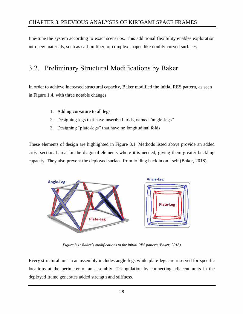
3.2. Preliminary Structural Modifications by Baker
In order to achieve increased structural capacity, Baker modified the initial RES pattern, as seen
in Figure 1.4, with three notable changes:
1. Adding curvature to all legs
2. Designing legs that have inscribed folds, named “angle-legs”
3. Designing “plate-legs” that have no longitudinal folds
These elements of design are highlighted in Figure 3.1. Methods listed above provide an added
cross-sectional area for the diagonal elements where it is needed, giving them greater buckling
capacity. They also prevent the deployed surface from folding back in on itself (Baker, 2018).
Figure 3.1: Baker’s modifications to the initial RES pattern (Baker, 2018)
Every structural unit in an assembly includes angle-legs while plate-legs are reserved for specific
locations at the perimeter of an assembly. Triangulation by connecting adjacent units in the
deployed frame generates added strength and stiffness.
CHAPTER 3. PREVIOUS ANALYSES OF KIRIGAMI SPACE FRAMES

29
3.3. Initial Structural Characterization of the
Spin-Valence Frame
The experimental testing and computational modeling yielded three significant behaviors for the
modified geometry:
1. Strain hardening of nodal components
2. Self-contact between Spin-Valence elements
3. Local buckling failure at primary and secondary surfaces
3.3.1. Strain Hardening of Nodal Components
Strain hardening, occurring at the ends of the angle-legs, contributed considerably to structural
capacity during loading. Angle-legs have their lowest cross-sectional areas in those sections,
causing them to be the first elements to yield, or reach stress values beyond the elastic region,
when the frame is subjected to progressively increasing loads. A unique property of steel is when
loaded beyond its elastic region, steel provides additional resistance until failure, a phenomenon
known as plastic strain hardening (Sherrow-Groves and Baker, 2019). Figure 3.2 illustrates an
approximated zone where plasticity occurs.
Figure 3.2: Strain hardening at kirigami unit nodes (Sherrow-Groves and Baker, 2019)
3.3. INITIAL STRUCTURAL CHARACTERIZATION OF THE SPIN-
VALENCE FRAME

30
Experimental testing observed that the redundancy of the triangulating legs will redistribute loads
when these nodes reach maximum capacity (Sahuc et al. 2019).
3.3.2. Self-contact Between System Elements
At the same interface mentioned above, another observation occurred post-buckling, instead of
post-yielding. Because of their lower cross-sectional area, those portions have a tendency to buckle
under axial loading. Sometimes, post-buckled angle-legs make contact with the primary surface
during loading as seen in Figure 3.3, adding significant strength to a yielded kirigami frame.
Contact between the angle-legs and the secondary surface, however, is more uncertain and cannot
be relied on (Sherrow-Groves and Baker, 2019).
Figure 3.3: Contact between angle-legs and primary surface (Sherrow-Groves and Baker, 2019)
3.3.3. Local Buckling Failure at Primary and Secondary Surfaces
Element buckling occurred mostly in the primary and secondary surfaces. Tensile and compressive
axial forces from the trusses activated this failure. This indicates that the angle-legs were over-
designed, as the distribution of stresses to the folded region was not as significant as anticipated.
Improved material allocations between the legs and surface elements were recommended for future
iterations (Sherrow-Groves and Baker, 2019).
CHAPTER 3. PREVIOUS ANALYSES OF KIRIGAMI SPACE FRAMES

31
Figure 3.4: Primary surface buckling failure (Sahuc et al., 2019)
3.4. Structural Recommendations
Prior analyses indicated that more efficient material allocation in the Spin-Valence design may be
possible. As mentioned in the previous section, angle-legs were slightly over-designed while the
primary and secondary surfaces experienced buckling. Therefore, future iterations of Spin-Valence
should CNC cut more steel into the surfaces instead of the legs. Moreover, modifying the geometry
to reliably force post-buckling self-contact from Section 3.2 will increase strength. Concluding
remarks from the laboratory and computational data also suggest that the tested system could
successfully be used in artistic structural installations but not yet suitable for spanning structures
(Sahuc et al., 2019; Sherrow-Groves and Baker, 2019).
To explore its architectural and structural benefits, this study looks into introducing double-
curvature to the Spin-Valence geometry. Similar to the spatial frame evolution from Section 2.1,
three-dimensionality or curvature traditionally enables more architectural versatility and structural
capacity to designs. Coupled with allowing input surfaces, the Spin-Valence system has the
potential to easily transport and construct structurally viable complex shells.
3.4. STRUCTURAL RECOMMENDATIONS

32
THIS PAGE INTENTIONALLY LEFT BLANK
CHAPTER 3. PREVIOUS ANALYSES OF KIRIGAMI SPACE FRAMES

33
Chapter 4
Preliminary Computational Modeling for
Deployment
This chapter examines Ramirez’s initial attempt at computationally modeling the deployment of
an individual Spin-Valence unit. The motivations behind computational modeling, the written
Grasshopper-based algorithm, and the results are discussed in this section.
4.1. Modeling Software
Geometry is defined in the CAD software, Rhinoceros v6 (Rhino), using the computational plug-
in Grasshopper for parametric design.
4.2. Motivation
As mentioned in Section 3.1, computational models enable users to discover more variable designs
without having to physically construct them. Prior to the following algorithms in Chapters 4-6, all
CAD configurations of Spin-Valence have been produced iteratively in Rhino. The methods
discussed below focus on creating a dynamic model from user-input parameters. Chapter 4

34
specifically explores generating a Spin-Valence unit using Grasshopper, allowing for adjustable
parameters such as unit sizing and deployment position.
Advancing from the traditionally flat kirigami frame to a doubly-curved surface requires
understanding NPPUs, or non-parallel plane units from Section 1.3.2. Flat or singly-curved
surfaces allow for both planes to remain relatively parallel, which can be easily modeled in a CAD
software. However, doubly-curved surfaces force the planes to be non-parallel, creating the tilting
effect seen in Figure 4.1. Figure 4.1 displays NPPUs compared to their counterparts PPUs, or
parallel plane units, using a 3D printed Spin-Valence model created by Emily Baker. Figure 5.3
showcases this model as well.
Figure 4.1: Parallel plane units (PPUs) vs. non-parallel plane units (NPPUs)
Therefore, properly understanding the deployment of a single unit is paramount to creating a fully
computational model. For user-variability and future optimization, unit deployment needs to be
controllable by modifiable parameters. The algorithm below describes a preliminary method for
solving the deployment of a Spin-Valence unit, using Grasshopper’s object-oriented software.
4.3. Base Unit Deployment Logic
This deployment logic is a 3D configuration-space for an individual unit. Input variables for this
CHAPTER 4. PRELIMINARY COMPUTATIONAL MODELING FOR
DEPLOYMENT
35
algorithm are polygon size, which can be adjusted freely using Grasshopper’s built-in sliders, and
the deployment parameters: ϴ, ϕ, and τ. The derivation for these parameters will be described in
Section 4.3.2. Moreover, polygons for this algorithm are limited to quads for simplification.
4.3.1. Constraints to the Problem
Spin-Valence’s design is deeply rooted in kirigami, so the computational model must adhere to
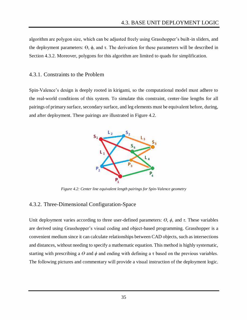
the real-world conditions of this system. To simulate this constraint, center-line lengths for all
pairings of primary surface, secondary surface, and leg elements must be equivalent before, during,
and after deployment. These pairings are illustrated in Figure 4.2.
Figure 4.2: Center line equivalent length pairings for Spin-Valence geometry
4.3.2. Three-Dimensional Configuration-Space
Unit deployment varies according to three user-defined parameters: ϴ, ϕ, and τ. These variables
are derived using Grasshopper’s visual coding and object-based programming. Grasshopper is a
convenient medium since it can calculate relationships between CAD objects, such as intersections
and distances, without needing to specify a mathematic equation. This method is highly systematic,
starting with prescribing a ϴ and ϕ and ending with defining a τ based on the previous variables.
The following pictures and commentary will provide a visual instruction of the deployment logic.
4.3. BASE UNIT DEPLOYMENT LOGIC
36
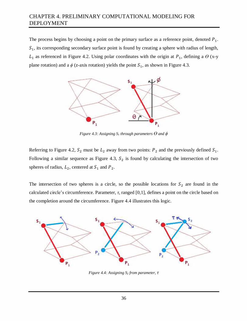
The process begins by choosing a point on the primary surface as a reference point, denoted 𝑃1.
𝑆1, its corresponding secondary surface point is found by creating a sphere with radius of length,
𝐿1 as referenced in Figure 4.2. Using polar coordinates with the origin at 𝑃1, defining a ϴ (x-y
plane rotation) and a ϕ (z-axis rotation) yields the point 𝑆1, as shown in Figure 4.3.
Figure 4.3: Assigning S1 through parameters ϴ and ϕ
Referring to Figure 4.2, 𝑆2 must be 𝐿2 away from two points: 𝑃2 and the previously defined 𝑆1.
Following a similar sequence as Figure 4.3, 𝑆2 is found by calculating the intersection of two
spheres of radius, 𝐿2, centered at 𝑆1 and 𝑃2.
The intersection of two spheres is a circle, so the possible locations for 𝑆2 are found in the
calculated circle’s circumference. Parameter, τ, ranged [0,1], defines a point on the circle based on
the completion around the circumference. Figure 4.4 illustrates this logic.
Figure 4.4: Assigning S2 from parameter, τ
CHAPTER 4. PRELIMINARY COMPUTATIONAL MODELING FOR
DEPLOYMENT

37
𝑆4 is found using the length relationships from Figure 4.2 and the same methodology of Figure
4.4. However, in this case, it includes the intersection of three spheres instead of two. Table 1
summarizes the specifications for all three spheres.
Table 1: Sphere specifications to locate S4
Sphere Center point Radius
1 𝑃4 𝐿4
2 𝑆1 𝐿1
3 𝑆2 𝐿2→4
First, the intersection of Spheres 2 and 3 are found, and once more, this yields a circle.
Radius, 𝐿2→4, is the distance between 𝑃2 and 𝑃4 on the primary surface. Finding where this newly
defined circle and Sphere 1 converge provides two point solutions. 𝑆4 is assigned to the point with
the greatest z-value because the other solution creates a non-constructible Spin-Valence
configuration.
Having 𝑆1, 𝑆2, and 𝑆4 generates the plane for the secondary surface. Using Grasshopper’s built-in
programs, creating circles around 𝑆2 and 𝑆4 with radii, 𝐿3 and 𝐿4 respectively, on the newly
constructed plane of the secondary surface, gives the coordinates for the final point, 𝑆3. Locating
the final points, 𝑆3 and 𝑆4 are illustrated in Figure 4.5.
Figure 4.5: Locating S4 from intersection of three spheres (left); locating S3 from planar relationships (right)
4.3. BASE UNIT DEPLOYMENT LOGIC

38
4.4. Algorithm Limitations and Transition
The algorithm, although functional, is restricted to a non-linear and discrete configuration-space.
Qualitative observations suggest that parameter, τ, is highly dependent on the combination of ϴ
and ϕ. Keeping τ consistent while changing ϴ and ϕ has the potential to create a non-constructible
or imaginary surface. This makes performing future optimization difficult due to the system’s non-
predictability.
Moreover, the algorithm is reliant on Grasshopper’s object-oriented programming. Translating
these intersections of 3D objects to mathematic equations becomes more complicated with every
equation introduced. For these reasons, research into finding a more mathematic-based deployment
algorithm is necessary to use optimization for generating a primary or secondary surface.
CHAPTER 4. PRELIMINARY COMPUTATIONAL MODELING FOR
DEPLOYMENT

39
Chapter 5
Mathematic Definition for Spin-Valence
Geometry Deployment
This chapter explores finding a mathematic definition for the deployment of an individual Spin-
Valence unit. Mathematic equations enable a better understanding of the system and have the
ability to be translated across software. The section below discusses the motivations for moving
past the initial Grasshopper algorithm and the derivation of the 2D configuration-space.
5.1. Motivation
As discussed in Section 4.2, understanding the deployment of a single Spin-Valence unit is integral
to generating a fully computational doubly-curved frame. Doubly-curved surfaces force their
primary and secondary planes to be non-parallel, so computational models must support these
configurations. Explained in Section 4.4, the previous method is unideal because it creates a
disjointed configuration-space and is too difficult to translate into other programs besides
Grasshopper.
Therefore, an entirely mathematic approach to solving deployment is optimal. These equations
would establish a more predictable configuration-space while being easily adapted to any matrix-
based coding language.
40
The following linear algebra proof is completed through collaborations between the University of
Arkansas and MIT. This derivation solves deployment as a 2D configuration-space instead of 3D
as first seen in Chapter 4 and works efficiently with rhombus shapes. Systems of equations and
simplifications are solved using Wolfram Mathematica v12.0 (Wolfram, 1988).
5.2. New Base Unit Deployment Logic
5.2.1. Notation
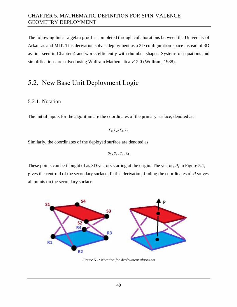
The initial inputs for the algorithm are the coordinates of the primary surface, denoted as:
𝑟1, 𝑟2, 𝑟3, 𝑟4
Similarly, the coordinates of the deployed surface are denoted as:
𝑠1, 𝑠2, 𝑠3, 𝑠4
These points can be thought of as 3D vectors starting at the origin. The vector, P, in Figure 5.1,
gives the centroid of the secondary surface. In this derivation, finding the coordinates of P solves
all points on the secondary surface.
Figure 5.1: Notation for deployment algorithm
CHAPTER 5. MATHEMATIC DEFINITION FOR SPIN-VALENCE
GEOMETRY DEPLOYMENT

41
The derivation in Section 5.2.3 refers to dot and cross products with the following notation:
Dot product: 𝑎. 𝑏
Cross: 𝑎 𝑥 𝑏
5.2.2. Mathematic Constraints
For consistency with real-world kirigami logic, the algorithm adheres to the same kirigami
constraints as Section 4.3.1. Center-line lengths in the primary surface, secondary surface, and leg
elements must be equivalent. Therefore, the following relationships, (1) and (2), hold true for all
length pairings in Figure 4.2.
Equation (1) ensures that the original side lengths are consistent in the secondary surface.
(𝑟1 − 𝑟2). (𝑟1 − 𝑟2) = (𝑠1 − 𝑠2). (𝑠1 − 𝑠2) = 𝑙1 (1)
Equation (2) forces diagonal leg lengths and side lengths to be equivalent.
(𝑠1 − 𝑟2). (𝑠1 − 𝑟2) = 𝑙1 (2)
Moreover, the algorithm currently works smoothly with only squares and rhombuses. Therefore,
𝑟1 = −𝑟3; 𝑟2 = −𝑟4 (3)
5.2.3. Solving the Deployment Equation for Parameters
The following proof solves the Spin-Valence deployment for a defined rhomb in a “local
coordinate system”. In the local system, the base geometry has its centroid at the origin, with its
rhomboidal primary and secondary axes along the x and y axes, respectively.
5.2. NEW BASE UNIT DEPLOYMENT LOGIC

42
The deployment relationship between the primary and secondary surface can be described with:
Side 1: 𝑠1 = 𝑅[𝑟1]
Side 2: 𝑠2 = 𝑅[𝑟2]
Side 3: 𝑠3 = 𝑅[𝑟3]
Side 4: 𝑠4 = 𝑅[𝑟4] (4)
Combining and simplifying (2) and (4) with Side 1:
(𝑠1 − 𝑟2). (𝑠1 − 𝑟2) =
(𝑅[𝑟1] − 𝑟2). (𝑅[𝑟1] − 𝑟2) =
𝑅[𝑟1]. 𝑅[𝑟1] − 2𝑅[𝑟1]. 𝑟2 + 𝑟2. 𝑟2 = 𝑙1 (5)
Transformation, 𝑅, is assumed to be an isometry, or a transformation that remains invariant with
respect to internal distances. In other words, applying 𝑅 does not change 𝑟1 and 𝑟2’s relationship
with one another. Now, (5) can be simplified with (1).
𝑅[𝑟1]. 𝑅[𝑟1] − 2𝑅[𝑟1]. 𝑟2 + 𝑟2. 𝑟2 = (𝑟1 − 𝑟2). (𝑟1 − 𝑟2)
𝑅[𝑟1]. 𝑅[𝑟1] − 2𝑅[𝑟1]. 𝑟2 + 𝑟2. 𝑟2 = 𝑟1. 𝑟1 − 2(𝑟2. 𝑟1) + 𝑟2. 𝑟2
𝑅[𝑟1]. 𝑅[𝑟1] − 2𝑅[𝑟1]. 𝑟2 = 𝑟1. 𝑟1 − 2(𝑟2. 𝑟1) (5a)
Applying (5a) to all sides in (4):
Side 1: 𝑅[𝑟1]. 𝑅[𝑟1] − 2𝑅[𝑟1]. 𝑟2 = 𝑟1. 𝑟1 − 2(𝑟2. 𝑟1)
Side 2: 𝑅[𝑟2]. 𝑅[𝑟2] − 2𝑅[𝑟2]. 𝑟3 = 𝑟2. 𝑟2 − 2(𝑟3. 𝑟2)
Side 3: 𝑅[𝑟3]. 𝑅[𝑟3] − 2𝑅[𝑟3]. 𝑟4 = 𝑟3. 𝑟3 − 2(𝑟4. 𝑟3)
Side 4: 𝑅[𝑟4]. 𝑅[𝑟4] − 2𝑅[𝑟4]. 𝑟1 = 𝑟4. 𝑟4 − 2(𝑟1. 𝑟4) (6)
CHAPTER 5. MATHEMATIC DEFINITION FOR SPIN-VALENCE
GEOMETRY DEPLOYMENT
43
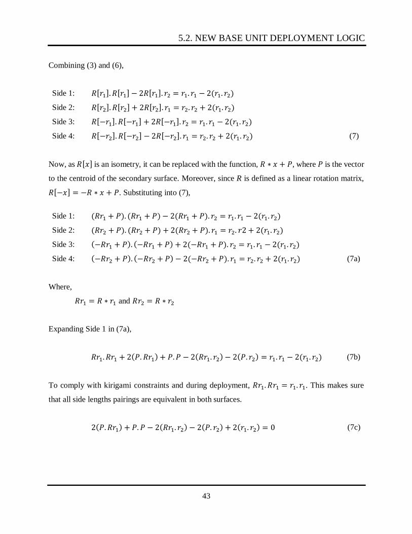
Combining (3) and (6),
Side 1: 𝑅[𝑟1]. 𝑅[𝑟1] − 2𝑅[𝑟1]. 𝑟2 = 𝑟1. 𝑟1 − 2(𝑟1. 𝑟2)
Side 2: 𝑅[𝑟2]. 𝑅[𝑟2] + 2𝑅[𝑟2]. 𝑟1 = 𝑟2. 𝑟2 + 2(𝑟1. 𝑟2)
Side 3: 𝑅[−𝑟1]. 𝑅[−𝑟1] + 2𝑅[−𝑟1]. 𝑟2 = 𝑟1. 𝑟1 − 2(𝑟1. 𝑟2)
Side 4: 𝑅[−𝑟2]. 𝑅[−𝑟2] − 2𝑅[−𝑟2]. 𝑟1 = 𝑟2. 𝑟2 + 2(𝑟1. 𝑟2) (7)
Now, as 𝑅[𝑥] is an isometry, it can be replaced with the function, 𝑅 ∗ 𝑥 + 𝑃, where 𝑃 is the vector
to the centroid of the secondary surface. Moreover, since R is defined as a linear rotation matrix,
𝑅[−𝑥] = −𝑅 ∗ 𝑥 + 𝑃. Substituting into (7),
Side 1: (𝑅𝑟1 + 𝑃). (𝑅𝑟1 + 𝑃) − 2(𝑅𝑟1 + 𝑃). 𝑟2 = 𝑟1. 𝑟1 − 2(𝑟1. 𝑟2)
Side 2: (𝑅𝑟2 + 𝑃). (𝑅𝑟2 + 𝑃) + 2(𝑅𝑟2 + 𝑃). 𝑟1 = 𝑟2. 𝑟2 + 2(𝑟1. 𝑟2)
Side 3: (−𝑅𝑟1 + 𝑃). (−𝑅𝑟1 + 𝑃) + 2(−𝑅𝑟1 + 𝑃). 𝑟2 = 𝑟1. 𝑟1 − 2(𝑟1. 𝑟2)
Side 4: (−𝑅𝑟2 + 𝑃). (−𝑅𝑟2 + 𝑃) − 2(−𝑅𝑟2 + 𝑃). 𝑟1 = 𝑟2. 𝑟2 + 2(𝑟1. 𝑟2) (7a)
Where,
𝑅𝑟1 = 𝑅 ∗ 𝑟1 and 𝑅𝑟2 = 𝑅 ∗ 𝑟2
Expanding Side 1 in (7a),
𝑅𝑟1. 𝑅𝑟1 + 2(𝑃. 𝑅𝑟1) + 𝑃. 𝑃 − 2(𝑅𝑟1. 𝑟2) − 2(𝑃. 𝑟2) = 𝑟1. 𝑟1 − 2(𝑟1. 𝑟2) (7b)
To comply with kirigami constraints and during deployment, 𝑅𝑟1. 𝑅𝑟1 = 𝑟1. 𝑟1. This makes sure
that all side lengths pairings are equivalent in both surfaces.
2(𝑃. 𝑅𝑟1) + 𝑃. 𝑃 − 2(𝑅𝑟1. 𝑟2) − 2(𝑃. 𝑟2) + 2(𝑟1. 𝑟2) = 0 (7c)
5.2. NEW BASE UNIT DEPLOYMENT LOGIC
44
Applying this constraint to all sides in (7):
Side 1: 2(𝑃. 𝑅𝑟1) + 𝑃. 𝑃 − 2(𝑅𝑟1. 𝑟2) − 2(𝑃. 𝑟2) + 2(𝑟1. 𝑟2) = 0
Side 2: 2(𝑃. 𝑅𝑟2) + 𝑃. 𝑃 + 2(𝑅𝑟2. 𝑟1) + 2(𝑃. 𝑟1) − 2(𝑟1. 𝑟2) = 0
Side 3: −2(𝑃. 𝑅𝑟1) + 𝑃. 𝑃 − 2(𝑅𝑟1. 𝑟2) + 2(𝑃. 𝑟2) + 2(𝑟1. 𝑟2) = 0
Side 4: −2(𝑃. 𝑅𝑟2) + 𝑃. 𝑃 + 2(𝑅𝑟2. 𝑟1) − 2(𝑃. 𝑟1) − 2(𝑟1. 𝑟2) = 0 (8)
Combining and simplifying the Sides in (8):
Eq. 1: (Side 1 - Side 3) 𝑃. 𝑅𝑟1 − 𝑃. 𝑟2 = 0
Eq. 2: (Side 2 - Side 4) 𝑃. 𝑅𝑟2 + 𝑃. 𝑟1 = 0
Eq. 3: (Side 1+ Side 3) 𝑃. 𝑃 + 2(𝑟1. 𝑟2) − 2(𝑅𝑟1. 𝑟2) = 0
Eq. 4: (Side 2+ Side 4) 𝑃. 𝑃 − 2(𝑟1. 𝑟2) + 2(𝑅𝑟2. 𝑟1) = 0 (9)
By restricting the solution to rhombuses, 𝑟1. 𝑟2 = 0. This simplifies (9) to:
Eq. 1: 𝑃. 𝑅𝑟1 − 𝑃. 𝑟2 = 0
Eq. 2: 𝑃. 𝑅𝑟2 + 𝑃. 𝑟1 = 0
Eq. 3a: 𝑃. 𝑃 − 2(𝑅𝑟1. 𝑟2) = 0
Eq. 4a: 𝑃. 𝑃 + 2(𝑅𝑟2. 𝑟1) = 0 (9a)
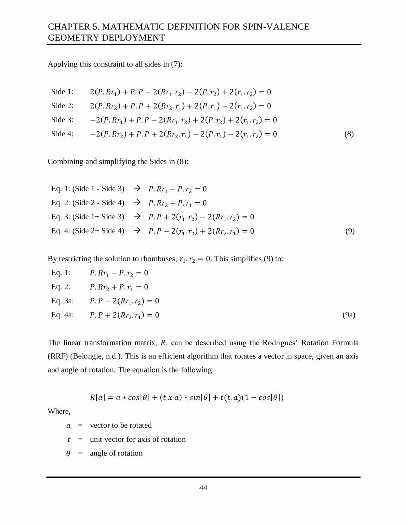
The linear transformation matrix, 𝑅, can be described using the Rodrigues’ Rotation Formula
(RRF) (Belongie, n.d.). This is an efficient algorithm that rotates a vector in space, given an axis
and angle of rotation. The equation is the following:
𝑅[𝑎] = 𝑎 ∗ 𝑐𝑜𝑠[𝜃] + (𝑡 𝑥 𝑎) ∗ 𝑠𝑖𝑛[𝜃] + 𝑡(𝑡. 𝑎)(1 − 𝑐𝑜𝑠[𝜃])
Where,
𝑎 = vector to be rotated
𝑡 = unit vector for axis of rotation
𝜃 = angle of rotation
CHAPTER 5. MATHEMATIC DEFINITION FOR SPIN-VALENCE
GEOMETRY DEPLOYMENT

45
Figure 5.2 labels these components and helps visualize the equation.
Figure 5.2: Rodrigues Rotation Formula notation (Dale, 2015)
Applying this formula to (9a),
Eq. 1: 𝑃. (−𝑟2 + 𝑟1 ∗ 𝑐𝑜𝑠[𝜃] + 𝑡(1 − 𝑐𝑜𝑠[𝜃])(𝑡. 𝑟1) + (𝑡 𝑥 𝑟1) ∗ 𝑠𝑖𝑛[𝜃]) = 0
Eq. 2: 𝑃. (𝑟1 + 𝑟2 ∗ 𝑐𝑜𝑠[𝜃] + 𝑡(1 − 𝑐𝑜𝑠[𝜃])(𝑡. 𝑟2) + (𝑡 𝑥 𝑟2) ∗ 𝑠𝑖𝑛[𝜃]) = 0
Eq. 3a: 𝑃. 𝑃 − 2 ∗ 𝑟2. (𝑟1 ∗ 𝑐𝑜𝑠[𝜃] + 𝑡(1 − 𝑐𝑜𝑠[𝜃])(𝑡. 𝑟1) + (𝑡 𝑥 𝑟1) ∗ 𝑠𝑖𝑛[𝜃]) = 0
Eq. 4a: 𝑃. 𝑃 + 2 ∗ 𝑟1. (𝑟2 ∗ 𝑐𝑜𝑠[𝜃] + 𝑡(1 − 𝑐𝑜𝑠[𝜃])(𝑡. 𝑟2) + (𝑡 𝑥 𝑟2) ∗ 𝑠𝑖𝑛[𝜃]) = 0 (10)
Combining Eq. 3a and Eq. 4a in (10) yields the following characteristic relationships:
Eq. 3a - Eq. 4a: (−1 + 𝑐𝑜𝑠[𝜃])(𝑡. 𝑟1)(𝑡. 𝑟2) = 0 (11)
Eq. 3a + Eq. 4a: 𝑃. 𝑃 − 2 ∗ 𝑟2. (𝑡 𝑥 𝑟1 ∗ 𝑠𝑖𝑛[𝜃]) = 0 (12)
(11) implies 3 cases: 𝜃 = 0, 𝑡. 𝑟1 = 0, or 𝑡. 𝑟2 = 0.
5.2. NEW BASE UNIT DEPLOYMENT LOGIC

46
5.2.3.1: Case 1 (𝜃 = 0):
If 𝜃 = 0, then (12) would simplify to the following:
𝑃. 𝑃 = 2 ∗ 𝑟2. (𝑡 𝑥 𝑟1 ∗ 𝑠𝑖𝑛[0])
𝑃. 𝑃 = 0
Recall that 𝑃. 𝑃 is the squared length of the vector to the centroid of the secondary surface. If
𝑃. 𝑃 = 0, then 𝜃 = 0 implies the non-deployed case, where the secondary surface is at the origin
while allowing the surface to tilt along its primary and secondary axes. Figure 5.3 depicts the 𝑟1
and 𝑟2 axes notation on a Spin-Valence unit. It also shows the tilting configurations in the non-
deployed case.
Figure 5.3: Notation for r1 and r2 axes (left); Non-deployed tilting along r1 axis (middle); tilting along r2 axis (right)
Therefore, fixing 𝜃 ≠ 0 and allowing 𝜃 to be an adjustable parameter enables the system to deploy
as the Spin-Valence geometry intended.
5.2.3.2: Cases 2 and 3 (𝑡. 𝑟1 = 0) or (𝑡. 𝑟2 = 0)
Cases 2 and 3 explore the relationships of 𝑡. 𝑟1 = 0 or 𝑡. 𝑟2 = 0. Referring to the notation in Figure
5.3, Case 2 allows for tilting along the 𝑟1 axis, while Case 3 accomplishes the same for the 𝑟2 axis.
The proofs for Case 2 and Case 3 are almost equivalent with the only notable differences, being
CHAPTER 5. MATHEMATIC DEFINITION FOR SPIN-VALENCE
GEOMETRY DEPLOYMENT

47
(13) and (14). Therefore, the following derivation only looks into Case 2, providing supplemental
commentary for Case 3. Case 3 is referred as the “b” equation.
𝑡. 𝑟1 = 0 (13)
𝑡. 𝑟2 = 0 (13b)
For (13) to be valid, 𝑡 must be a 1x3 matrix or vector that is perpendicular to 𝑟1. Since 𝑟1 is defined
is defined in the local coordinate system, 𝑡 can be denoted as follows:
𝑡 = [0 𝑠𝑖𝑛 [𝜑] 𝑐𝑜𝑠 [𝜑]] (14)
𝑡𝑏 = [𝑠𝑖𝑛 [𝜑] 0 𝑐𝑜𝑠 [𝜑]] (14b)
Defining 𝑡 with 𝑠𝑖𝑛 [𝜑] and 𝑐𝑜𝑠 [𝜑] allows for 𝑡 to be consistent as a unit vector, while introducing
variability for the y and z directions with only one parameter, 𝜑.
Plugging (14) into (12) and assigning a 𝜃 and φ gives the squared length of 𝑃, the distance to the
deployed surface’s centroid. Vector, 𝑃, can be solved through a system of equations, using 𝑃. 𝑃
and Equations 1 and 2 of (10). Section 6.5.7 and the Mathematica file in Appendix A detail the
exact methodology for solving the system.
Modifying (4) with the RRF and the isometry relationship, the exact secondary surface vertices
can be derived.
Side 1: 𝑠1 = 𝑅[𝑟1] = 𝑟1 ∗ 𝑐𝑜𝑠[𝜃] + (𝑡 𝑥 𝑟1) ∗ 𝑠𝑖𝑛[𝜃] + 𝑡(𝑡. 𝑟1)(1 − 𝑐𝑜𝑠[𝜃]) + 𝑃
Side 2: 𝑠2 = 𝑅[𝑟2] = 𝑟2 ∗ 𝑐𝑜𝑠[𝜃] + (𝑡 𝑥 𝑟2) ∗ 𝑠𝑖𝑛[𝜃] + 𝑡(𝑡. 𝑟2)(1 − 𝑐𝑜𝑠[𝜃]) + 𝑃
Side 3: 𝑠3 = 𝑅[𝑟3] = 𝑟3 ∗ 𝑐𝑜𝑠[𝜃] + (𝑡 𝑥 𝑟3) ∗ 𝑠𝑖𝑛[𝜃] + 𝑡(𝑡. 𝑟3)(1 − 𝑐𝑜𝑠[𝜃]) + 𝑃
Side 4: 𝑠4 = 𝑅[𝑟4] = 𝑟4 ∗ 𝑐𝑜𝑠[𝜃] + (𝑡 𝑥 𝑟4) ∗ 𝑠𝑖𝑛[𝜃] + 𝑡(𝑡. 𝑟4)(1 − 𝑐𝑜𝑠[𝜃]) + 𝑃 (4a)
5.2. NEW BASE UNIT DEPLOYMENT LOGIC

48
To summarize, these vertices can be found by giving the parameters, θ and φ, and specifying
whether performing Case 2 or 3.
A sample calculation using the parameters:
θ = 0.5
φ = 0.25
is available in Appendix B, using Mathematica.
CHAPTER 5. MATHEMATIC DEFINITION FOR SPIN-VALENCE
GEOMETRY DEPLOYMENT

49
Chapter 6
Algorithms for Computational Primary and
Secondary Surface Generation
With a mathematic algorithm for deployment, doubly-curved Spin-Valence frames can now be
modeled computationally. To review, introducing double-curvature to Spin-Valence forces its
primary and secondary surfaces to become non-parallel. Therefore, an algorithm that can create
NPPUs through adjustable parameters is necessary.
Having equations to describe deployment produces a more predictable configuration-space for
optimization. Creating the primary surface through optimization, covered in Section 6.5, is
contingent on this more navigable space.
This chapter overviews a workflow for generating a complete Spin-Valence frame from input
surfaces, based on research by a team of collaborators at MIT, the University of Arkansas (Emily
Baker and Edmund Harriss), and Arup (Nick Sherrow-Groves).
6.1. Modeling Software
Input surfaces are defined in Rhinoceros v6 (Rhino), using the computational plug-in Grasshopper
for parametric design. Grasshopper’s Kangaroo physics simulator is used for the secondary surface

50
generation. Python v3.7 is used to calculate an optimized primary surface that is deployed from
data obtained for the secondary surface. The library SciPy is used for optimization in this step.
6.2. Motivation
As introduced in Section 1.4, accurate computational models extend the Spin-Valence geometry
to allow input surfaces. This design freedom unlocks the system’s capabilities to handle various
boundary conditions and loading scenarios. Double-curvature, as seen in Chapter 2, strengthens
spanning systems, giving Spin-Valence more opportunity for use as a long-spanning spatial
structure for temporary bridges, vaults, or roofing.
The workflow is this chapter presents a systematic procedure to create complex geometries from
Spin-Valence. Surface generation is semi-automatic, letting users pursue creativity while requiring
little to no effort.
6.3. Proposed Workflow for Constructing a
Doubly-Curved Pavilion
The project team has created a workflow to generate a fully constructed doubly-curved pavilion,
which was proposed to be displayed at the International Shell and Spatial Structures (IASS) 2020
Symposium. The abstract for the related publication, co-authored by Baker, Harriss, Herning,
Ramirez, and Sherrow-Groves and entitled "DCSV Pavilion: Double-Curved Spin-Valence Space
Frame," has been accepted by the IASS 2020 Symposium committee. However, the IASS 2020
Symposium was postponed due to a global health crisis (IASS, 2020). It is expected that the paper
will be presented at the IASS 2021 Symposium.
CHAPTER 6. ALGORITHMS FOR COMPUTATIONAL PRIMARY AND
SECONDARY SURFACE GENERATION

51
Design and construction of the pavilion aims to showcase the advancements in Spin-Valence,
featuring computational modeling, finite element analysis, and doubly-curved surface
construction.
The proposed workflow for creating the pavilion is as follows:
1. User-generated surface in Rhino
2. Secondary surface generation using Grasshopper
3. Primary surface optimization in Python
4. Final meshing in Rhino
5. Finite Element Analysis of Pavilion
6.3.1. User-generated surfaces
Input surfaces are created by manipulating the geometry of 6 curves in Rhino. Each of these curves
are modifiable by control points, able to be moved anywhere in the 3D space. The group of curves
are then lofted in Grasshopper, or approximated into a surface. Figure 6.1 displays the proposed
input curves for the IASS design, and Figure 6.2 depicts the final approximated surface from the
input curves.
Figure 6.1: Input curves for surface generation
6.3. PROPOSED WORKFLOW FOR CONSTRUCTING A DOUBLY-CURVED
PAVILION

52
Figure 6.2: Formulated surface from input curves
In Section 6.3.2, a hard constraint generating the secondary surface are the boundaries highlighted
in blue in Figure 6.3. Physically, these two edge curves represent the structural supports in the
system. The left most curve is pin-supported throughout its entire length while the right-most curve
is pin-supported only along the units in front. This poses an interesting stress distribution
throughout the space frame which will be investigated in the finite element analysis in Chapter 7.
Figure 6.3: Boundary conditions for input surface (highlighted in blue)
6.3.2. Grasshopper-Produced Secondary Surface
Referenced in Chapter 1, the kirigami frame receives its rigidity from its triangulating legs,
resembling that of a spatial truss. Building this formation requires adjacent units to be connected
on both surfaces. The secondary surface due to the Spin-Valence geometry has a fixed amount of
material. Meanwhile, the primary surface has more flexibility because material can always be
added to its exterior.
CHAPTER 6. ALGORITHMS FOR COMPUTATIONAL PRIMARY AND
SECONDARY SURFACE GENERATION

53
Therefore, the more constrained secondary surface will be created first, directly from the input
geometry. The primary surface will then be deployed from the secondary, using the algorithm from
Chapter 5. Optimization is performed to make these deployed units infinitesimally close to one
another. Final meshing in Rhino appends the needed material to create a cohesive layer, forming
the internal truss network.
To produce the secondary surface, a Grasshopper script is created to decompose the input geometry
in Figure 6.2 into a grid as seen in Figure 6.4.
Figure 6.4: Grid-pattern of secondary surface
Next, the gridded surface is converted to a highly controlled, secondary surface configuration
through optimization in Kangaroo. The optimization, explained in Section 6.4, aims to create an
accurate 45° Pythagorean tiling while staying consistent with Figure 6.2. Individual unit data and
the dimensions of the pavilion in Figure 6.5 are then sent to Python to calculate a primary surface,
using optimization once more.
Figure 6.5: Optimized Pythagorean tiling of secondary surface
6.3. PROPOSED WORKFLOW FOR CONSTRUCTING A DOUBLY-CURVED
PAVILION

54
6.3.3. Optimized Deployed Primary Surface
The Grasshopper data is then translated into Python, where the following process is explained in
more detail in Section 6.5. Individual primary surface units are deployed from their secondary
counterparts using the algorithm in Chapter 5. To summarize, parameters, θ and φ, dictate each
unit’s final position according to mathematic relationships.
Optimization, using the SciPy library in Python, is used to construct a buildable primary surface.
The objective value for this optimization are the distances between deployed units. The optimizer
minimizes this value by altering the parameter matrix of θ’s and φ’s to find a local minimum in
the 2N configuration-space, with N being the total number of units. Figure 6.6 displays an example
primary surface that will be exported to Rhino for final meshing.
Figure 6.6: Optimized primary surface
6.3.4. Final Meshed Model in Rhino
A new Grasshopper script receives the Python data for both surfaces and creates the pavilion using
those returned points. This last step in Rhino unites any separated units through steel point
connections as seen in Figure 6.7.
CHAPTER 6. ALGORITHMS FOR COMPUTATIONAL PRIMARY AND
SECONDARY SURFACE GENERATION
55
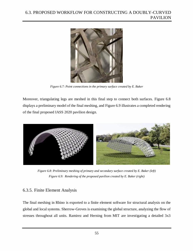
Figure 6.7: Point connections in the primary surface created by E. Baker
Moreover, triangulating legs are meshed in this final step to connect both surfaces. Figure 6.8
displays a preliminary model of the final meshing, and Figure 6.9 illustrates a completed rendering
of the final proposed IASS 2020 pavilion design.
Figure 6.8: Preliminary meshing of primary and secondary surface created by E. Baker (left)
Figure 6.9: Rendering of the proposed pavilion created by E. Baker (right)
6.3.5. Finite Element Analysis
The final meshing in Rhino is exported to a finite element software for structural analysis on the
global and local systems. Sherrow-Groves is examining the global structure, analyzing the flow of
stresses throughout all units. Ramirez and Herning from MIT are investigating a detailed 3x3
6.3. PROPOSED WORKFLOW FOR CONSTRUCTING A DOUBLY-CURVED
PAVILION

56
assembly of the most stressed boundary condition. Figure 6.10 showcases a preliminary
computational test in Abaqus 2017 (ABAQUS, 1978).
Figure 6.10: Abaqus finite element model of 3x3 assembly
6.4. Computationally Produced Secondary Surface
The preliminary version for modeling kirigami frames from input surfaces was created by Baker
and Harriss (Baker and Harriss, n.d.). Their work references initial influences from Song’s study
of modeling reciprocal frames from user generated surfaces (Song et al., 2014). However, the
algorithm’s main inspiration comes from the original Pythagorean tiling method mentioned in
Chapter 1.
The original Grasshopper algorithm has since been modified through collaborations with Ramirez.
After creating an input surface, the program divides the mesh into a grid. These individual quads
are the foundational pieces to perform optimization.
Forming a cohesive secondary surface requires hard constraints detailed in Section 6.4.1. The
constraints for this system can be thought of as springs – “the further they are from the ideal
position, the harder they pull” (Baker and Harriss, n.d.). That allows this problem to be
CHAPTER 6. ALGORITHMS FOR COMPUTATIONAL PRIMARY AND
SECONDARY SURFACE GENERATION

57
reconfigured for Kangaroo, a physics simulator in Grasshopper. Kangaroo uses optimization under
these constraints to convert the gridded surface into the prescribed 45° Pythagorean tiling, as
illustrated in Figure 6.11. More details on the optimization are described in the ongoing paper,
titled “Double-Curved Spin-Valence: Geometric and Computational Basis,” for the upcoming
Advances in Architectural Geometry (AAG) 2020 conference.
Figure 6.11: Secondary surface generated from input surface (Baker and Harriss, n.d.)
6.4.1. Constraints
The constraints in the Kangaroo script originate from qualitative observations of the doubly-curved
frames. As referenced in Section 4.2, doubly-curved Spin-Valence units have a non-parallel
internal geometry. However, having near parallel units is preferable for strength and structural
redundancy. To achieve this while respecting the input geometry, connected units must spread
local deformations smoothly along the surface while remaining somewhat parallel.
This can be accomplished through optimization in Kangaroo by having strict constraints for the
positions of each unit’s vertices. These mathematic constraints can be summarized as:
A) Neighboring units meet at their corners
B) Vertices must stay close to the target surfaces
C) Edge curves (Figure 6.3) are hard boundaries that cannot be passed
D) Individual units must be rhomboidal
6.4. COMPUTATIONALLY PRODUCED SECONDARY SURFACE

58
More details regarding the derivation of constraints A, B, and C are found in the ongoing AAG
2020 paper. Constraint D is a revision to Harriss’s initial Grasshopper script due to the deployment
logic in Chapter 5 requiring rhomboidal units.
Figures 6.4 and 6.5 depict the input surface before and after optimization with Kangaroo.
6.4.2. Transition to Python-produced Primary Surface
After optimization, individual unit data is transferred to Python to compute the primary surface.
The exported data includes two pieces of information:
1. Global tiling data
2. Unit rhombus specifications
Figure 6.12: Global tiling specifications
Global tiling data details the number of units in all rows, P, and columns, Q. This gives the total
number of units, N, by multiplying P with Q. Unit rhombus specifications are the center points,
vectors to units’ first corners, and vectors to units’ second corners for every rhombus in the
pavilion.
CHAPTER 6. ALGORITHMS FOR COMPUTATIONAL PRIMARY AND
SECONDARY SURFACE GENERATION

59
6.5. Optimized Deployment of Primary Surface
The primary surface deployment script in Python is produced at MIT with coordination from PI,
Gordana Herning. It can be subdivided into five main functions: File_read, Objective, Kirigami,
Distance, and Plot.
To summarize, File_read imports Grasshopper data and divides it into usable matrices. Objective
loops through all units and runs the Kirigami and Distance functions. Kirigami simulates local unit
deployment according to parameters, θ and φ. Next, Objective stores all units’ final primary and
secondary surface positions and sends this information to Distance. Distance returns the objective
value for optimization by summing the distances between all adjacent units.
SciPy’s minimize function performs optimization on the structure. It modifies the Distance outputs
by incrementally changing the θ and φ parameters for each unit. Plot illustrates the final
configuration.
6.5.1. Imported Python libraries
The Python libraries used in this section are: NumPy, SciPy, and Matplotlib. NumPy and SciPy
are used for basic math functions in Python. SciPy has a built in optimizer that will be used in
Section 6.5.4. Matplotlib plots the final outcome of the optimization.
6.5.2. Notation
All variables in the Python script are located in Appendix C and defined by comments. There are
multiple 4x3 matrices that represent different versions of the primary and secondary surface
vertices. Figure 6.13 illustrates the notation of an individual unit. Each corner is represented by a
row in their respective 4x3 matrix.
6.5. OPTIMIZED DEPLOYMENT OF PRIMARY SURFACE

60
Figure 6.13: Labeled primary and secondary vertices
Notice the differences between Figures 5.1 and 6.13. Figure 6.13 shows the primary surface
deploying from its secondary counterpart, as mentioned in Section 6.3.2.
For this script, the points switch between a global and an arbitrary local coordinate system. The
deployment algorithm from Chapter 5 is successful if the non-deployed rhombs meet two
conditions:
1. Non-deployed rhombs are centered at the origin
2. Primary and secondary rhomboidal axes are along the x and y axes
To distinguish between the matrices in the different coordinate axes, matrices are labeled the
following:
pl = primary surface in local
pgb = primary surface in global before expansion factor
pg = primary surface in global after expansion factor
sl = secondary surface in local
sgd = secondary surface input data for Kirigami
sg = secondary surface in global
CHAPTER 6. ALGORITHMS FOR COMPUTATIONAL PRIMARY AND
SECONDARY SURFACE GENERATION

61
The vector, P, remains the same as Chapter 5, as seen in Figure 5.1. It has been renamed to 𝑝𝑙𝑐𝑒𝑛
in the Python script for clarity. Similar to Chapter 5, solving for 𝑝𝑙𝑐𝑒𝑛 gives the deployed primary
surface vertices in the local system.
6.5.3. Parameters
Parameters for the algorithm are the Grasshopper data file, the θ and φ matrices, and the primary
surface expansion factor, exp.
Section 6.5.4 discusses deconstructing the Grasshopper inputs into the pavilion dimensions and
individual unit data. θ and φ are arbitrary Nx1 matrices and are the same parameters derived from
Chapter 5. These will be used as the base parameters for optimization. Exp enlarges the deployed
rhomb by an assigned ratio after reaching its final position. This attempts to accurately represent
the shifted center-line geometries due to real-life leg thicknesses. Figure 6.14 depicts this offset.
Figure 6.14: Offset center-line geometry
6.5.4. Optimization
For specific surfaces, like spheres, connections between adjacent units can be investigated
analytically and adjusted to form perfect solutions. However, the more complex, input surfaces
cannot yield a direct solution due to the amount of variation involved (Gelfand and Silverman,
6.5. OPTIMIZED DEPLOYMENT OF PRIMARY SURFACE

62
2000). Therefore, optimization is used to incrementally find a near-ideal solution. Simple
unconstrained optimization techniques require two inputs: an objective function, f, and adjustable
parameters. More complex forms involve the Jacobian (first derivative of f), Hessian (second
derivative of f), and parameter constraints.
The main method for this script’s optimization is gradient descent, which modifies its parameters
based on the local slope of the configuration-space. It makes small improvements until it reaches
a threshold value, ε, or exceeds the set number of iterations. If the objective value differs by less
than ε per iteration, the optimizer reaches convergence and returns the final objective value.
In this script, f is defined as the Objective function, where the objective value is the summation of
distances between adjacent units, which is calculated in Distance. The optimizer minimizes these
distances by modifying the parameters θ and φ for each unit.
6.5.5. File_read
Before use in Python, the exported Grasshopper data from Section 6.4 is slightly modified. All
data from Grasshopper is exported as one text file for simplicity. File_Read decomposes and
reformats this data into three matrices, as referenced in Section 6.4.2.
The first two rows of exported data are P and Q, which detail the number of units in each row and
column in the pavilion. N is the total number of units, found by multiplying P and Q. Being a 2D
configuration-space, this script contains 2N number of parameters.
The remaining rows are the rhombus data for every unit in the pavilion. Every 3 rows in the matrix
represents a new unit, specifying global vectors for the base polygon’s origin, primary axis, and
secondary axis. The data for an individual unit is termed, sgd, which stands for “secondary global
unit data”.
CHAPTER 6. ALGORITHMS FOR COMPUTATIONAL PRIMARY AND
SECONDARY SURFACE GENERATION

63
6.5.6. Objective
As referenced in Section 6.5.4, the objective function, f, minimizes the total distance between
adjacent units by modifying the parameters, θ and φ. Objective organizes the received data from
File_Read into N individual units with matrix size 3x3. Objective then loops N number of times
and transfers the individual unit data, sgd, alongside that unit’s assigned θ and φ values to the
function Kirigami. Afterwards, Objective compiles a matrix of all global primary and secondary
coordinates returned from Kirigami.
These final global positions are stored in two 4Nx3 matrices, denoted as primary and secondary.
The primary matrix is transferred to Distance to calculate the optimizer’s objective value. This
final value is returned to the SciPy optimizer where the total distance will be minimized. The
final product will create a more cohesive, constructible primary surface.
6.5.7. Kirigami
The function, Kirigami, models single unit deployment according to the following variables: 𝑠𝑔𝑑,
θ, and φ. Referenced in Section 6.5.5, 𝑠𝑔𝑑 is a matrix composed of a rhomb’s global centroid
position and vectors for its primary and secondary axes, titled 𝑠𝑔𝑝 and 𝑠𝑔𝑠.
𝑠𝑔𝑑 = [
𝑠𝑔𝑐𝑒𝑛
𝑠𝑔𝑝
𝑠𝑔𝑠
] (15)
Where,
𝑠𝑔𝑐𝑒𝑛 = coordinates of polygon centroid
𝑠𝑔𝑝 = vector along rhombus primary axis
𝑠𝑔𝑠 = vector along rhombus secondary axis
The global coordinates of the secondary surface are calculated and stored in the matrix, 𝑠𝑔.
6.5. OPTIMIZED DEPLOYMENT OF PRIMARY SURFACE

64
𝑠𝑔 = [
𝑠𝑔𝑐𝑒𝑛 + 𝑠𝑔𝑝
𝑠𝑔𝑐𝑒𝑛 + 𝑠𝑔𝑠
𝑠𝑔𝑐𝑒𝑛 − 𝑠𝑔𝑝
𝑠𝑔𝑐𝑒𝑛 − 𝑠𝑔𝑠
]
(16)
As stated in Section 6.5.2, the Python script switches between a global and an arbitrary local
coordinate system. The algorithm from Chapter 5 is successful only in this newly created local
system. Therefore, 𝑠𝑔 must be converted into a 4x3 matrix, named 𝑠𝑙, containing the local
coordinates of the secondary surface’s corners. To do this, the Euclidean distances of vectors 𝑠𝑔𝑝
and 𝑠𝑔𝑠 are calculated and stored as 𝑝𝑙𝑒𝑛 and 𝑠𝑙𝑒𝑛 respectively. The 𝑠𝑙 matrix is calculated in (17).
𝑠𝑙 = [
𝑝𝑙𝑒𝑛 0 00 𝑠𝑙𝑒𝑛 0
−𝑝𝑙𝑒𝑛 0 00 −𝑠𝑙𝑒𝑛 0
]
(17)
From Chapter 5, calculating the deployment of the primary surface requires 3 variables: a base
polygon, and parameters θ and φ. To recap, these variables solve a system of equations that gives,
the vector, P, renamed 𝑝𝑙𝑐𝑒𝑛, as seen in Figure 5.1. The Rodrigues Rotation Formula (RRF)
alongside 𝑝𝑙𝑐𝑒𝑛 equates the final local position of the deployed primary surface. Equations (10),
(11), (12), and (14) from Chapter 5 are used in the following algorithm.
First, using the Case 2 assumption of 𝑡. 𝑟1 = 0 in (11), (14) is used to establish the unit vector for
the axis of rotation in the RRF.
(−1 + 𝑐𝑜𝑠[𝜃])(𝑡. 𝑟1)(𝑡. 𝑟2) = 0 (11)
𝑡 = [0 𝑠𝑖𝑛 [𝜑] 𝑐𝑜𝑠 [𝜑]] (14)
Where,
r1 = [𝑠𝑙11 𝑠𝑙12 𝑠𝑙13]
r2 = [𝑠𝑙21 𝑠𝑙22 𝑠𝑙23]
CHAPTER 6. ALGORITHMS FOR COMPUTATIONAL PRIMARY AND
SECONDARY SURFACE GENERATION

65
Rearranging (12) equates the magnitude of vector 𝑝𝑙𝑐𝑒𝑛, ‖𝑝𝑙𝑐𝑒𝑛‖:
‖𝑝𝑙𝑐𝑒𝑛‖ = √𝑝𝑙𝑐𝑒𝑛 . 𝑝𝑙𝑐𝑒𝑛 = √2 ∗ 𝑟2. (𝑡 𝑥 𝑟1 ∗ 𝑠𝑖𝑛[𝜃]) (18)
To solve for the vector, 𝑝𝑙𝑐𝑒𝑛, finding its i, j, and k components is necessary. This requires a
system of three equations to solve completely.
One equation can be derived through the distance formula.
𝑖2 + 𝑗2 + 𝑘2 = ‖𝑝𝑙𝑐𝑒𝑛‖2 (19)
The other two can be obtained from (10).
𝑝𝑙𝑐𝑒𝑛 . (−𝑟2 + 𝑟1 ∗ 𝑐𝑜𝑠[𝜃] + 𝑡(1 − 𝑐𝑜𝑠[𝜃])(𝑡. 𝑟1) + (𝑡 𝑥 𝑟1) ∗ 𝑠𝑖𝑛[𝜃]) = 0 (10a)
𝑝𝑙𝑐𝑒𝑛 . (𝑟1 + 𝑟2 ∗ 𝑐𝑜𝑠[𝜃] + 𝑡(1 − 𝑐𝑜𝑠[𝜃])(𝑡. 𝑟2) + (𝑡 𝑥 𝑟2) ∗ 𝑠𝑖𝑛[𝜃]) = 0 (10b)
Since 𝑟2, 𝑟1, θ, and 𝑡 are known, the parenthetical regions can be rewritten as constants:
𝐴 = −𝑟2 + 𝑟1 ∗ 𝑐𝑜𝑠[𝜃] + 𝑡(1 − 𝑐𝑜𝑠[𝜃])(𝑡. 𝑟1) + (𝑡 𝑥 𝑟1) ∗ 𝑠𝑖𝑛[𝜃] (20)
𝐵 = 𝑟1 + 𝑟2 ∗ 𝑐𝑜𝑠[𝜃] + 𝑡(1 − 𝑐𝑜𝑠[𝜃])(𝑡. 𝑟2) + (𝑡 𝑥 𝑟2) ∗ 𝑠𝑖𝑛[𝜃] (21)
Substituting,
𝑝𝑙𝑐𝑒𝑛 . 𝐴 = 0 (10ai)
𝑝𝑙𝑐𝑒𝑛 . 𝐵 = 0 (10bi)
Where vectors, A and B, are notated,
A = [𝐴𝑥 𝐴𝑦 𝐴𝑧]
B = [𝐵𝑥 𝐵𝑦 𝐵𝑧]
6.5. OPTIMIZED DEPLOYMENT OF PRIMARY SURFACE

66
Expanding (10ai) and (10bi) gives the last two equations to solve for i, j, and k,
𝐴𝑥 ∗ 𝑖 + 𝐴𝑦 ∗ 𝑗 + 𝐴𝑧 ∗ 𝑘 = 0 (10aii)
𝐵𝑥 ∗ 𝑖 + 𝐵𝑦 ∗ 𝑗 + 𝐵𝑧 ∗ 𝑘 = 0 (10bii)
This system of equations is solved in Wolfram Mathematica and the exact solution for i, j, and k
is located in Appendix A.
The locations of each vertex in the local coordinate system can be found by modifying (4) with
the isometry relationship and the RRF.
Side 1: 𝑝1 = 𝑅[𝑠1] = 𝑠1 ∗ 𝑐𝑜𝑠[𝜃] + (𝑡 𝑥 𝑠1) ∗ 𝑠𝑖𝑛[𝜃] + 𝑡(𝑡. 𝑠1)(1 − 𝑐𝑜𝑠[𝜃]) + 𝑝𝑙𝑐𝑒𝑛
Side 2: 𝑝2 = 𝑅[𝑠2] = 𝑠2 ∗ 𝑐𝑜𝑠[𝜃] + (𝑡 𝑥 𝑠2) ∗ 𝑠𝑖𝑛[𝜃] + 𝑡(𝑡. 𝑠2)(1 − 𝑐𝑜𝑠[𝜃]) + 𝑝𝑙𝑐𝑒𝑛
Side 3: 𝑝3 = 𝑅[𝑠3] = 𝑠3 ∗ 𝑐𝑜𝑠[𝜃] + (𝑡 𝑥 𝑠3) ∗ 𝑠𝑖𝑛[𝜃] + 𝑡(𝑡. 𝑠3)(1 − 𝑐𝑜𝑠[𝜃]) + 𝑝𝑙𝑐𝑒𝑛
Side 4: 𝑝4 = 𝑅[𝑠4] = 𝑠4 ∗ 𝑐𝑜𝑠[𝜃] + (𝑡 𝑥 𝑠4) ∗ 𝑠𝑖𝑛[𝜃] + 𝑡(𝑡. 𝑠4)(1 − 𝑐𝑜𝑠[𝜃]) + 𝑝𝑙𝑐𝑒𝑛 (4a)
This is stored in the matrix, pl:
𝑝𝑙 = [
𝑝1
𝑝2
𝑝3
𝑝4
]
(22)
To convert these newly found points from the local to global coordinate systems, another
transformation matrix, G, must be calculated. This is found by compiling the unit vectors that make
up the desired global axis and organizing them in the following manner:
𝐺 = [
𝑠𝑔𝑝
𝑠𝑔𝑠
𝑠𝑔𝑝 𝑥 𝑠𝑔𝑠
] (23)
CHAPTER 6. ALGORITHMS FOR COMPUTATIONAL PRIMARY AND
SECONDARY SURFACE GENERATION

67
Performing the transformation:
Side 1: 𝑝𝑔𝑏1 = 𝑝1 ∗ 𝐺 + 𝑠𝑔𝑐𝑒𝑛
Side 2: 𝑝𝑔𝑏2 = 𝑝2 ∗ 𝐺 + 𝑠𝑔𝑐𝑒𝑛
Side 3: 𝑝𝑔𝑏3 = 𝑝3 ∗ 𝐺 + 𝑠𝑔𝑐𝑒𝑛
Side 4: 𝑝𝑔𝑏4 = 𝑝4 ∗ 𝐺 + 𝑠𝑔𝑐𝑒𝑛 (24)
Similarly,
𝑝𝑔𝑐𝑒𝑛 = 𝑝𝑙𝑐𝑒𝑛 ∗ 𝐺 + 𝑠𝑔𝑐𝑒𝑛 (25)
For the primary surface to accurately represent real-world construction, a primary surface
expansion factor, exp, is introduced. This ratio takes into account the offset between the secondary
surface and primary surface that is created during the CNC cut. Figure 6.14 shows a graphical
depiction of this. To solve for the new vertex positions, the linear relationship below is used:
Side 1: 𝑝𝑔1 = 𝑝𝑔𝑏1 + 𝑒𝑥𝑝 ∗𝑝𝑔𝑏1 − 𝑝𝑔𝑐𝑒𝑛
‖𝑝𝑔𝑏1 − 𝑝𝑔𝑐𝑒𝑛‖
Side 2: 𝑝𝑔2 = 𝑝𝑔𝑏2 + 𝑒𝑥𝑝 ∗𝑝𝑔𝑏2 − 𝑝𝑔𝑐𝑒𝑛
‖𝑝𝑔𝑏2 − 𝑝𝑔𝑐𝑒𝑛‖
Side 3: 𝑝𝑔3 = 𝑝𝑔𝑏3 + 𝑒𝑥𝑝 ∗𝑝𝑔𝑏3 − 𝑝𝑔𝑐𝑒𝑛
‖𝑝𝑔𝑏3 − 𝑝𝑔𝑐𝑒𝑛‖
Side 4: 𝑝𝑔4 = 𝑝𝑔𝑏4 + 𝑒𝑥𝑝 ∗𝑝𝑔𝑏4 − 𝑝𝑔𝑐𝑒𝑛
‖𝑝𝑔𝑏4 − 𝑝𝑔𝑐𝑒𝑛‖
(26)
Aggregating gives the final global coordinates for the primary surface,
𝑝𝑔 = [
𝑝𝑔1
𝑝𝑔2
𝑝𝑔3
𝑝𝑔4
]
(27)
6.5. OPTIMIZED DEPLOYMENT OF PRIMARY SURFACE

68
6.5.8. Distance
Distance calculates the objective value for optimization by summing the distances between
adjacent units. The function requires three parameters: P, Q, and primary. It will receive these
parameters from Objective after all units have undergone the Kirigami function.
There are two principal matrices in this operation: orient and xn. Orient stands for orientation and
is a QxP matrix that numbers off unit positions in the global structure. Figure 6.15 illustrates the
numbering of the matrix, orient.
Figure 6.15: Orient matrix numbering notation
𝑜𝑟𝑖𝑒𝑛𝑡 = [
1 ⋯ 𝑃⋮ ⋱ ⋮
𝑄 ∗ (𝑃 − 1) + 1 ⋯ 𝑄 ∗ 𝑃]
(28)
Xn is a Nx4 matrix that determines the adjacent units for an individual rhomb based on its position
in orient. To begin, the algorithm operates on an arbitrary notation that assigns a matrix column to
a specific side on the rhomb. This is depicted in Figure 6.16.
CHAPTER 6. ALGORITHMS FOR COMPUTATIONAL PRIMARY AND
SECONDARY SURFACE GENERATION

69
Figure 6.16: Notation for assigning sides to columns in xn matrix
To simplify, in the xn matrix, columns correspond to the following sides:
Table 2: Simplified legend for Figure 6.16
Column Side Segment
1 Bottom P1 P2
2 Left P2 P3
3 Top P3 P4
4 Right P4 P1
The script loops through all of the units in orient and examines its current position. From here, the
program finds the numbers adjacent to its current position and assigns those adjacent numbers to
a column based on the notation in Figure 6.16.
Noticing patterns in the connections of the orient matrix, xn follows 5 basic rules. These rules are
shown in Table 3.
6.5. OPTIMIZED DEPLOYMENT OF PRIMARY SURFACE

70
Table 3: Xn matrix rules
Position in orient Column
in xn
Row of
Adjacent Unit
Column of
Adjacent Unit
Rows after the first 3 Row above Same
Rows before the last 1 Row below Same
Columns right of the first 2 Same Column left
Columns left of the last 4 Same Column right
Moreover, sides without an adjacent unit are assigned 0 in their respective columns. Figure 6.17
displays an example output script in Windows Powershell with a sample orient and xn for more
clarification.
Figure 6.17: Sample orient (left) and xn (right) matrices for a 4x4 assembly
After setting up xn, the script establishes a relationship between the xn and primary matrices to
calculate adjacent unit distances. It accomplishes this by following the flowchart in Figure 6.18.
CHAPTER 6. ALGORITHMS FOR COMPUTATIONAL PRIMARY AND
SECONDARY SURFACE GENERATION
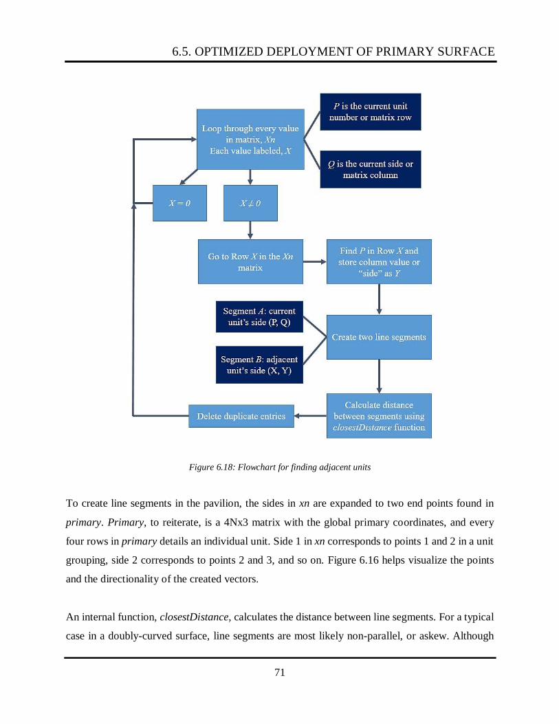
71
Figure 6.18: Flowchart for finding adjacent units
To create line segments in the pavilion, the sides in xn are expanded to two end points found in
primary. Primary, to reiterate, is a 4Nx3 matrix with the global primary coordinates, and every
four rows in primary details an individual unit. Side 1 in xn corresponds to points 1 and 2 in a unit
grouping, side 2 corresponds to points 2 and 3, and so on. Figure 6.16 helps visualize the points
and the directionality of the created vectors.
An internal function, closestDistance, calculates the distance between line segments. For a typical
case in a doubly-curved surface, line segments are most likely non-parallel, or askew. Although
6.5. OPTIMIZED DEPLOYMENT OF PRIMARY SURFACE

72
the parallel case is coded in the script for security purposes, it will not be explored in this paper.
The typical non-parallel case in closestDistance is explained below.
For this algorithm, the current side, titled A, will have end points, 𝑎0 and 𝑎1, and the adjacent side,
titled B, will be have end points, 𝑏0 and 𝑏1. This allows us to represent A and B as:
𝐴 = 𝑎1 − 𝑎0 (29a)
𝐵 = 𝑏1 − 𝑏0 (29b)
The strategy behind finding the distance between 2 askew lines is to find two parallel planes
passing through each line. Distance between the planes is calculated using vector projection as
seen in equation (30).
𝑑𝑖𝑠𝑡 =
(𝐴 𝑥 𝐵). (𝑏0 − 𝑎0)
‖𝐴 𝑥 𝐵‖
(30)
However, equation (30) assumes infinite length vectors instead of finite segments like A and B.
Therefore, for the closest points, 𝑐1 (line A) and 𝑐2 (line B), it has to be verified whether they are
within the bounds of the segments. If not, then the endpoints of the line segments are assumed as
the new closest points.
The closest points, 𝑐1 and 𝑐2, are calculated in equations (31a) and (31b).
𝑐1 = 𝑎0 +
(𝑏0 − 𝑎0). (𝐵𝑢 𝑥 𝑛)
𝐴𝑢 . (𝐵𝑢 𝑥 𝑛)∗ 𝐴𝑢
(31a)
𝑐2 = 𝑏0 +
(𝑎0 − 𝑏0). (𝐴𝑢 𝑥 𝑛)
𝐵𝑢 . (𝐴𝑢 𝑥 𝑛)∗ 𝐵𝑢
(31b)
Where,
𝐴𝑢 = unit vector of segment A
CHAPTER 6. ALGORITHMS FOR COMPUTATIONAL PRIMARY AND
SECONDARY SURFACE GENERATION

73
𝐵𝑢 = unit vector of segment B
𝑛 = cross product of 𝐴𝑢 and 𝐵𝑢
To determine whether 𝑐1 and 𝑐2 are within Sides A and B, the script uses a mathematic relationship,
knowing that they are points along their corresponding infinite vectors.
𝑐1 = 𝑎0 + 𝑡1 ∗ 𝐴𝑢 (32a)
𝑐2 = 𝑏0 + 𝑡2 ∗ 𝐵𝑢 (32b)
Where,
𝑡1 = constant to describe position along Side A
𝑡2 = constant to describe position along Side B
Since 𝑐1 − 𝑎0 is proportional to 𝐴𝑢, any coordinate in both matrices are proportional to each other.
This yields two ratios to solve for 𝑐1 and 𝑐2, where subscript, x, represents the x-coordinate.
𝑡1 =
(𝑐1 − 𝑎0)𝑥
𝐴𝑢𝑥
(32ai)
𝑡2 =
(𝑐2 − 𝑏0)𝑥
𝐵𝑢𝑥
(32bi)
Figure 6.19 distinguishes the different possibilities for the final closest points pA and pB, with the
boundary conditions included.
6.5. OPTIMIZED DEPLOYMENT OF PRIMARY SURFACE

74
Figure 6.19: pA and pB combinations including segment boundary conditions
If 𝑡1 and 𝑡2 are within 0 to ‖𝐴‖ or ‖𝐵‖ respectively, then:
pA = c1 = a0 + t1 ∗ Au (33a)
pB = c2 = b0 + t2 ∗ Bu (33b)
The final distance is calculated by taking the norm of (pB − pA). This number is returned back to
Objective for later optimization.
t1
< 0 pA = a0 B.(a0-b0)
< 0 pB = 0
> 0 , < ||B|| pB = b0 + B*B.(a0-b0)
> ||B|| pB = b0 + B*||B||
> ||A|| pA = a1 B.(a1-b0)
< 0 pB = 0
> 0 , < ||B|| pB = b0 + B*B.(a1-b0)
> ||B|| pB = b0 + B*||B||
t2
< 0 pB = b0 A.(b0-a0)
< 0 pA = 0
> 0 , < ||A|| pA = a0 + A*A.(b0-a0)
> ||A|| pA = a0 + A*||A||
> ||B|| pB = b1 A.(b1-a0)
< 0 pA = 0
> 0 , < ||A|| pA = a0 + A*A.(b1-a0)
> ||A|| pA = a0 + A*||A||
CHAPTER 6. ALGORITHMS FOR COMPUTATIONAL PRIMARY AND
SECONDARY SURFACE GENERATION

75
6.5.9. Plot
Plot is a 3D plotter using the Axis3d plug-in within the Matplotlib library. This displays the
global secondary surface, augmented primary surface, and the triangulating legs in 3D. This step
is to help with mathematic validation and visual aesthetics. Figure 6.20 displays an example of
the final configuration after optimization.
Figure 6.20: Plot example using Axis3d
6.5.10. Results
The goal for this section is to formulate an efficient workflow that creates a doubly-curved,
deployed primary surface. To produce a constructible deployed layer, optimization is used to
connect all units in the primary surface by incrementally changing set parameters derived in
Chapter 5.
The SciPy library comes equipped with several algorithms for optimization, and to produce the
best results, or models with the smallest objective value, these different methods are tested and
modeled. More images of these results are located in Appendix D.
6.5. OPTIMIZED DEPLOYMENT OF PRIMARY SURFACE
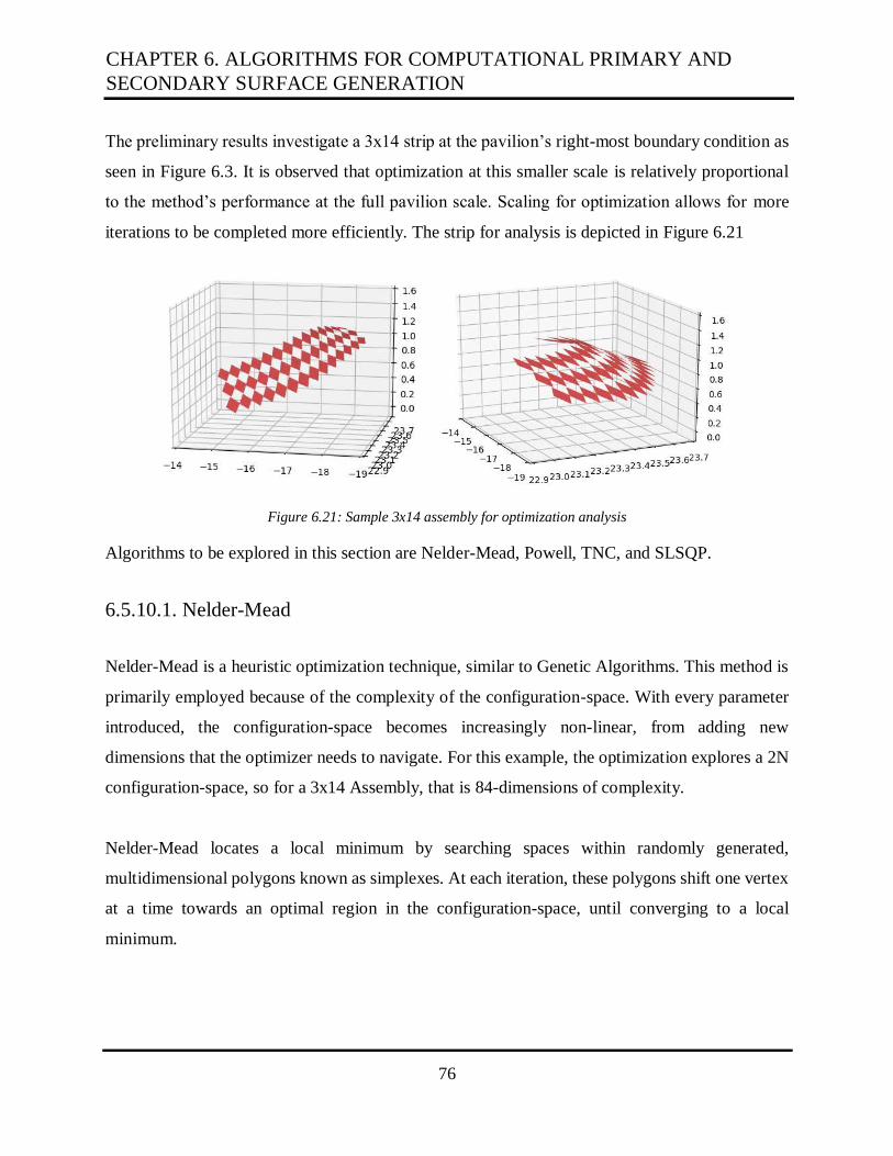
76
The preliminary results investigate a 3x14 strip at the pavilion’s right-most boundary condition as
seen in Figure 6.3. It is observed that optimization at this smaller scale is relatively proportional
to the method’s performance at the full pavilion scale. Scaling for optimization allows for more
iterations to be completed more efficiently. The strip for analysis is depicted in Figure 6.21
Figure 6.21: Sample 3x14 assembly for optimization analysis
Algorithms to be explored in this section are Nelder-Mead, Powell, TNC, and SLSQP.
6.5.10.1. Nelder-Mead
Nelder-Mead is a heuristic optimization technique, similar to Genetic Algorithms. This method is
primarily employed because of the complexity of the configuration-space. With every parameter
introduced, the configuration-space becomes increasingly non-linear, from adding new
dimensions that the optimizer needs to navigate. For this example, the optimization explores a 2N
configuration-space, so for a 3x14 Assembly, that is 84-dimensions of complexity.
Nelder-Mead locates a local minimum by searching spaces within randomly generated,
multidimensional polygons known as simplexes. At each iteration, these polygons shift one vertex
at a time towards an optimal region in the configuration-space, until converging to a local
minimum.
CHAPTER 6. ALGORITHMS FOR COMPUTATIONAL PRIMARY AND
SECONDARY SURFACE GENERATION

77
Figure 6.22: Nelder-Mead optimization results
Table 4: Nelder-Mead Optimization Results
Case theta phi exp # of iterations initial distance final distance % reduction
Nelder-Mead 0.5 0.01 0.075 5000 2.628 1.683 35.95%
The heuristic approach has a reduction of 35.95%. Moreover, the final result displayed in Figure
6.22 has a relatively smooth deployed surface, barring a couple of inconsistencies especially at the
boundaries. Downsides to using the Nelder-Mead method are its long computational time and its
exploration of a relatively small configuration-space, which is reflected by its small percent
reduction.
6.5.10.2. Powell
Powell method is a gradient descent optimizer. Gradient descent optimizers take small steps in the
configuration-space in the direction of the current gradient, or the direction of steepest descent. It
will continue taking steps in that direction unless the objective value increases or converges. By
taking the gradient, the optimization converges faster to a solution than the traditional heuristic
approach taken by the Nelder-Mead method.
6.5. OPTIMIZED DEPLOYMENT OF PRIMARY SURFACE
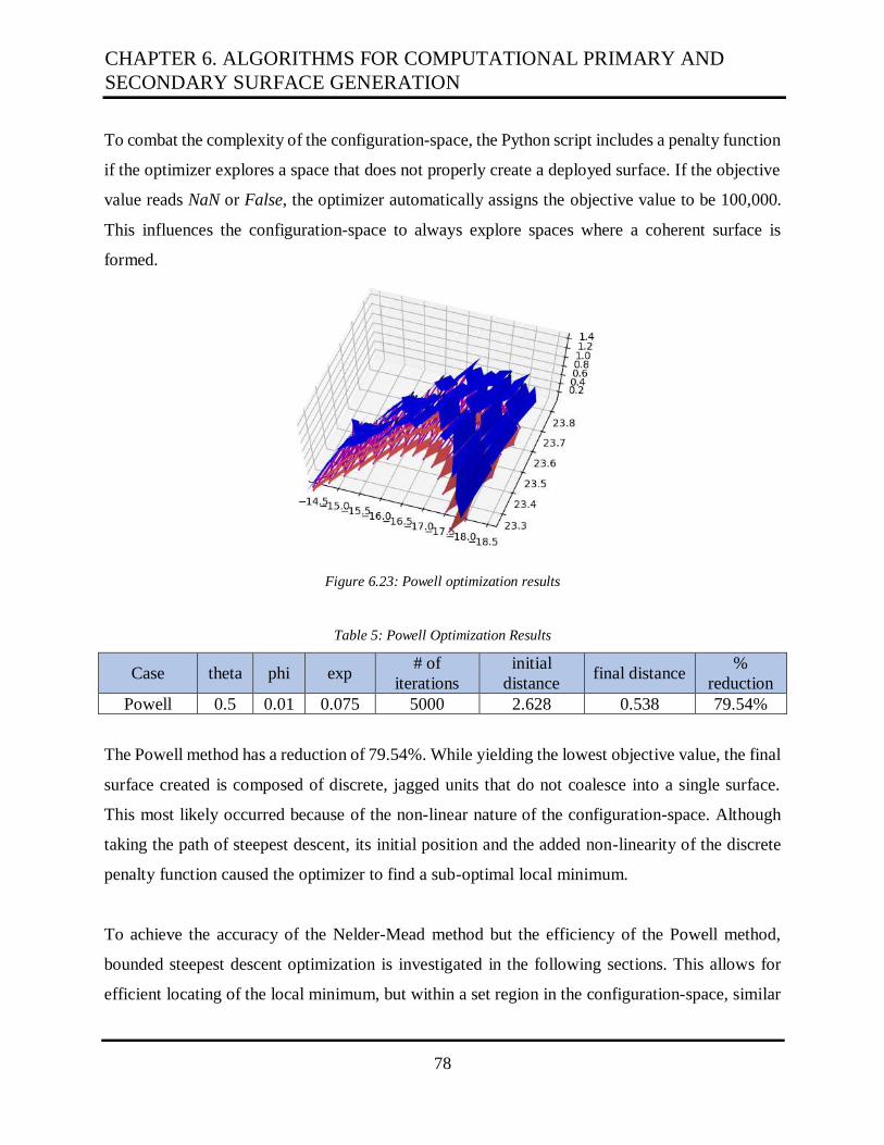
78
To combat the complexity of the configuration-space, the Python script includes a penalty function
if the optimizer explores a space that does not properly create a deployed surface. If the objective
value reads NaN or False, the optimizer automatically assigns the objective value to be 100,000.
This influences the configuration-space to always explore spaces where a coherent surface is
formed.
Figure 6.23: Powell optimization results
Table 5: Powell Optimization Results
Case theta phi exp # of
iterations
initial
distance final distance
%
reduction
Powell 0.5 0.01 0.075 5000 2.628 0.538 79.54%
The Powell method has a reduction of 79.54%. While yielding the lowest objective value, the final
surface created is composed of discrete, jagged units that do not coalesce into a single surface.
This most likely occurred because of the non-linear nature of the configuration-space. Although
taking the path of steepest descent, its initial position and the added non-linearity of the discrete
penalty function caused the optimizer to find a sub-optimal local minimum.
To achieve the accuracy of the Nelder-Mead method but the efficiency of the Powell method,
bounded steepest descent optimization is investigated in the following sections. This allows for
efficient locating of the local minimum, but within a set region in the configuration-space, similar
CHAPTER 6. ALGORITHMS FOR COMPUTATIONAL PRIMARY AND
SECONDARY SURFACE GENERATION

79
to the heuristic method. Two methods in SciPy that allow for bounded, unconstrained optimization
without a Jacobian or Hessian function are TNC and SLSQP.
6.5.10.3. TNC (Truncated Newton Conjugate-Gradient)
The Truncated Newton Conjugate-Gradient, or TNC, optimizer uses the Newton method for
finding local minimums. Newton method is an extended version of the gradient descent optimizer
used in the Powell method. It includes a more refined way of reaching a minimum that molds its
steps better to more naturally navigate the configuration-space. Figure 6.24 depicts this
mathematic phenomenon.
Figure 6.24: Steepest descent (blue) vs. Newton method (black) for locating local minima
Moreover, this method is preferred because it is “truncated.” SciPy’s TNC algorithm allows users
to incorporate assigned bounds for its parameters, limiting the explored configuration-space to
create a more constructible surface.
Therefore, three different bounds cases are explored, adjusting 𝜃 and 𝜑’s navigable space. These
cases alongside their objective values are shown in Figure 6.25 and Table 6.
6.5. OPTIMIZED DEPLOYMENT OF PRIMARY SURFACE

80
Figure 6.25: TNC 1: Theta [.301,.800], Phi [.001,.5] (left),
TNC 2: Theta [.301,.900], Phi [.001,.6] (middle),
TNC 3: Theta [.401,.900], Phi [.001,.5] (right)
Table 6: TNC Optimization Results
Case theta phi exp # of
iterations
initial
distance
final
distance
%
reduction
TNC 1 0.301 - 0.8 0.001 - 0.5 0.075 100 2.724 1.457 46.48%
TNC 2 0.301 - 0.9 0.001 - 0.6 0.075 100 2.724 1.432 47.40%
TNC 3 0.401 - 0.9 0.001 - 0.5 0.075 100 2.724 1.210 53.92%
As observed by Table 6, the highest percent reduction came from the bounds with the highest theta
values, TNC Case 3 being the largest with Case 2 as second. Moreover, referring to Figure 6.25,
Case 3 has the smoothest primary surface created with Case 1 following. These results depict that
the configuration-space rewards higher theta values with a greater percent reduction, but punishes
having a wider range, creating non-uniform meshes in the primary surface.
6.5.10.4. SLSQP (Sequential Least Squares Programming)
The same case study for bounds is investigated with the Sequential Least Squares Programming,
or SLSQP, optimization method in SciPy. SLSQP is a nonlinear optimizer that incorporates the
Newton method logic from Section 6.5.10.3 and the Broyden-Fletcher-Goldfarb-Shanno (BFGS)
algorithm. BFGS is a numerical Hessian function update strategy that helps with optimization. The
findings for the bounded SLSQP study are represented in Figure 6.26 and Table 7.
CHAPTER 6. ALGORITHMS FOR COMPUTATIONAL PRIMARY AND
SECONDARY SURFACE GENERATION
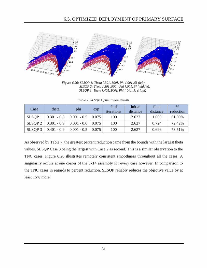
81
Figure 6.26: SLSQP 1: Theta [.301,.800], Phi [.001,.5] (left), SLSQP 2: Theta [.301,.900], Phi [.001,.6] (middle),
SLSQP 3: Theta [.401,.900], Phi [.001,.5] (right)
Table 7: SLSQP Optimization Results
Case theta phi exp # of
iterations
initial
distance
final
distance
%
reduction
SLSQP 1 0.301 - 0.8 0.001 - 0.5 0.075 100 2.627 1.000 61.89%
SLSQP 2 0.301 - 0.9 0.001 - 0.6 0.075 100 2.627 0.724 72.42%
SLSQP 3 0.401 - 0.9 0.001 - 0.5 0.075 100 2.627 0.696 73.51%
As observed by Table 7, the greatest percent reduction came from the bounds with the largest theta
values, SLSQP Case 3 being the largest with Case 2 as second. This is a similar observation to the
TNC cases. Figure 6.26 illustrates remotely consistent smoothness throughout all the cases. A
singularity occurs at one corner of the 3x14 assembly for every case however. In comparison to
the TNC cases in regards to percent reduction, SLSQP reliably reduces the objective value by at
least 15% more.
6.5. OPTIMIZED DEPLOYMENT OF PRIMARY SURFACE

82
6.5.10.5. Summary of 3x14 Assembly Optimization Case Study
Table 8: Summary of 3x14 Assembly Optimization Results
Case theta phi exp # of
iterations
initial
distance
final
distance
%
reduction
Nelder-
Mead 0.5 0.01 0.075 5000 2.628 1.683 35.95%
Powell 0.5 0.01 0.075 5000 2.628 0.538 79.54%
TNC 1 0.301 - 0.8 0.001 - 0.5 0.075 100 2.724 1.457 46.48%
TNC 2 0.301 - 0.9 0.001 - 0.6 0.075 100 2.724 1.432 47.40%
TNC 3 0.401 - 0.9 0.001 - 0.5 0.075 100 2.724 1.210 53.92%
SLSQP 1 0.301 - 0.8 0.001 - 0.5 0.075 100 2.627 1.000 61.89%
SLSQP 2 0.301 - 0.9 0.001 - 0.6 0.075 100 2.627 0.724 72.42%
SLSQP 3 0.401 - 0.9 0.001 - 0.5 0.075 100 2.627 0.696 73.51%
6.5.10.6. Final Pavilion
The final pavilion is modeled using both the TNC and SLSQP methods. TNC noticeably gives a
cleaner, smoother primary surface while SLSQP yields a consistently lower objective value. This
experiment will be conducted using Case 3 in both methods. Figure 6.27 shows the non-optimized
primary surface before running the Python script.
Figure 6.27: Pavilion design prior to optimization
CHAPTER 6. ALGORITHMS FOR COMPUTATIONAL PRIMARY AND
SECONDARY SURFACE GENERATION

83
Figures 6.28 and 6.29 display the optimized pavilion using the TNC and SLSQP methods
respectively. Table 9 shows the final values for both optimization methods.
Figure 6.28: TNC optimization for proposed pavilion design
Figure 6.29: SLSQP optimization for proposed pavilion design
Table 9: Proposed Pavilion Optimization Results
Case theta phi exp # of
iterations
initial
distance
final
distance
%
reduction
TNC 0.401 - 0.9 0.001 - 0.5 0.075 100 25.351 15.219 39.97%
SLSQP 0.401 - 0.9 0.001 - 0.5 0.075 100 25.351 9.847 61.17%
Table 9 reflects the observations found Section 6.5.10.4, where the SLSQP method has a percent
reduction almost 20% greater than the TNC method. In other words, deployed units are closer
together, creating a more idealized primary surface. Figures 6.28 and 6.29 both display relatively
6.5. OPTIMIZED DEPLOYMENT OF PRIMARY SURFACE

84
smooth optimized surfaces, with no one method seemingly more advantageous than the other.
Therefore, for future optimization of the finalized pavilion design, the SLSQP algorithm from the
SciPy library will be utilized.
6.5.11. Improvements for the Future
Two main modifications should be looked into for future installments of the Python script in
Section 6.5. The optimizer currently used in SciPy is non-modifiable, so having a built-in optimizer
within the Python code allows for more variability depending on the current conditions of the
problem. Moreover, equating a Jacobian or Hessian function for Objective is another step that
allows for more efficient optimization. Currently, the SciPy packages calculate approximations for
both values; therefore, having an analytical way to describe the gradient will enhance the
performance of the system.
CHAPTER 6. ALGORITHMS FOR COMPUTATIONAL PRIMARY AND
SECONDARY SURFACE GENERATION

85
Chapter 7
Finite Element Analysis of Proposed Pavilion
Design
This chapter discusses performing finite element analysis on a computationally formed doubly-
curved pavilion to investigate its structural behavior. Computational analysis is required due to
compounding the already complex Spin-Valence geometry with double-curvature.
Recent computational analysis of the kirigami frame by Sherrow-Groves and Baker (2019) has
been continued for the proposed pavilion design as noted in Chapter 6. Computational analysis is
conducted through a collaborative effort between Arup and MIT. Sherrow-Groves is investigating
the global effects of loading on the structure, specifically looking at the global stress distributions
and behavior related to construction and support conditions.
The thesis author has investigated the original computational model (Baker and Sherrow-Groves,
2019) in order to numerically analyze, using Abaqus, the local effects of a particular section of the
pavilion. Upon validating the model created using Abaqus based on results of prior analyses
(Sherrow-Groves and Baker, 2019) (Sahuc et al., 2019), the goal of the present study is to create a
detailed 3x3 unit assembly of the pavilion section shown in Figure 7.1. The aim of this study is to
understand the effect of stress distributions on connection behavior at the most highly stressed
section of the pavilion.
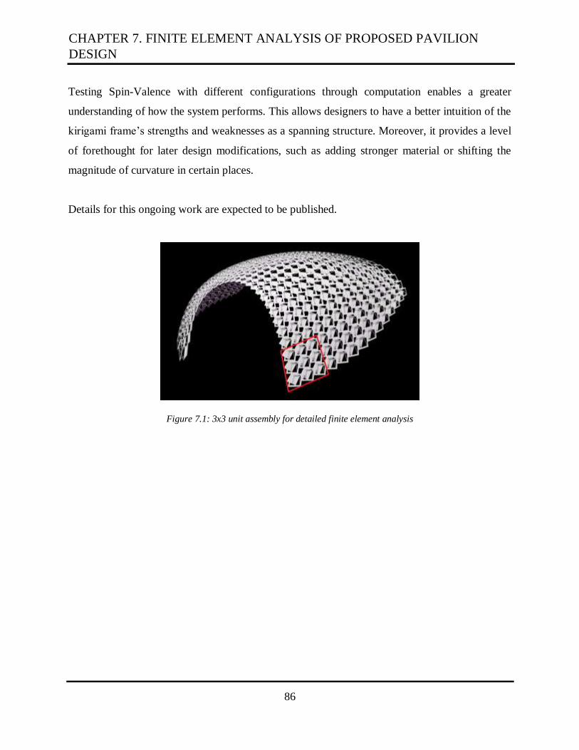
86
Testing Spin-Valence with different configurations through computation enables a greater
understanding of how the system performs. This allows designers to have a better intuition of the
kirigami frame’s strengths and weaknesses as a spanning structure. Moreover, it provides a level
of forethought for later design modifications, such as adding stronger material or shifting the
magnitude of curvature in certain places.
Details for this ongoing work are expected to be published.
Figure 7.1: 3x3 unit assembly for detailed finite element analysis
CHAPTER 7. FINITE ELEMENT ANALYSIS OF PROPOSED PAVILION
DESIGN

87
Chapter 8
Conclusion
This chapter summarizes the work presented in this MEng thesis and discusses the next steps for
deployable Spin-Valence spatial frames. It also reiterates the potential impacts this ongoing
research may achieve.
8.1. Summary of Contributions
The derivation for the deployment of an individual Spin-Valence unit has been found. It solves the
system as a 2D configuration-space.
A preliminary workflow has been proposed to translate input surfaces from Rhino to fully realized,
doubly-curved kirigami spatial frames.
A modified algorithm for forming the secondary surface in Grasshopper from input surfaces has
been achieved through collaborations between Harriss and Ramirez.
Using the mathematic deployment algorithm, a cohesive primary surface can be formulated in
Python using the Sequential Least Squares Programming, or SLSQP, optimization method in
SciPy.

88
A model of the flat 3x3 unit assembly has been set up in Abaqus for validation based on the prior
numerical study (Sherrow-Groves and Baker, 2019). It is used to supplement the analysis of
connection behavior in a 3x3 unit section extracted from the pavilion structure.
8.2. Future Work
In terms of geometry, the algorithm derived in this thesis grants a better mathematic understanding
of the Spin-Valence system. It can be used to extend the kirigami configurations beyond
rhombuses to parallelograms or other polygons. Current projects that are being discussed are
triangular or hexagonal space frames or geodesic domes created using the Spin-Valence pattern
logic.
As mentioned in Section 6.5.11, optimization can be improved by programming a built-in
optimizer within the Python script that does not rely on the SciPy library or configuring Jacobian
and Hessian equations for the objective function. These modifications would enable greater system
variability and computational speed.
The final results of the verification model along with the local 3x3 subassembly of the pavilion are
expected to be published in the paper entitled “DCSV Pavilion: Double-Curved Spin-Valence
Space Frame,” and presented at the IASS 2021 Symposium. Investigation of structural behavior
of doubly-curved Spin-Valence frames is important for developing new configurations for the
frame. Understanding global and local stress distributions, buckling modes, and behavior will
provide better intuition for creating more efficient Spin-Valence frames. Improvements in the
computational and structural analysis domains of kirigami spatial frames can make Spin-Valence
a more viable concept in the field of deployable mechanisms.
CHAPTER 8. CONCLUSION
89
8.3. Concluding Remarks and Potential Impacts
This thesis derives a new way of extending the Spin-Valence pattern logic to doubly-curved input
surfaces. Introducing curvature to the originally flat design enables the kirigami frame to
counterbalance internal element forces with better material efficiency and architecturally
variability. By creating a simplistic workflow that generates fully computational Spin-Valence
models, users have greater freedom to express their creativity whether they are producing
structural art installments or solving interesting boundary conditions using the kirigami
deployment method.
With Spin-Valence being a deployable mechanism, these creations can be easily transported and
deployed to a variety of locations. Hopefully, the Spin-Valence kirigami spatial frames will be
used in practice to create beautiful and economic forms in the built environment.
8.3. CONCLUDING REMARKS AND POTENTIAL IMPACTS

90
THIS PAGE INTENTIONALLY LEFT BLANK
CHAPTER 8. CONCLUSION

91
Chapter 9
References
ABAQUS Inc. (1978). SIMULIA Abaqus FEA.
Addis, B. (2006, Mar). The Crystal Palace and its place in stuctural history. International
Journal of Space Structures, 21, 3-19.
Baker, E. (2014). Search for a Rooted Aesthetic: Study in Spin-Valence. In F. Gramazio, M.
Kohler, & S. Langenberg (Ed.), Fabricate: Negotiating Design & Making, (pp. 128-135).
Zurich, Switzerland.
Baker, E. (2018). Spin-Valence: Kirigami Space Frame. In C. Mueller, & S. Adriaenssens (Ed.),
IASS Symposium 2018, Creativity in Structural Design, (pp. 1-7(7)). International
Association for Shell and Spatial Structures.
Baker, E., & Harriss, E. (n.d.). Computational Method for Mapping Kirigami Space Frames onto
Input Surfaces. (manuscript in preparation)
Belongie, S. (n.d.). Rodrigues' Rotation Formula. MathWorld - A Wolfram Web Resource.
WolfRam Research, Inc.
Beorkem, C. (2013). Flatform. Material Strategies in Digital Fabrication, 85-89.
Eureka. (2014). Rapid Deployable System (RDS).
Gelfand, I., & Silverman, R. (2000). Calculus of Variations. Chelmsford, MA: Courier
Corporation.
Gore, N. (2004). Craft and Innovation: Serious Play and the Direct Experience of the Real.
Journal of Architectural Education, 58(1), 39-44.
Hanaor, A., & Levy, R. (2001). Evaluation of deployable structures for space enclosures.
International Journal of Space Structures, 16, 221-229.
Hiroshima University. (2015). PreAssemble type of Bridge: Mobile Bridge. Hiroshima.
92
International Association of Shell and Spatial Structures. (2020). IASS ANNUAL SYMPOSIUM
AND SPATIAL STRUCTURES CONFERENCE 2020. Retrieved from
https://www.surrey.ac.uk/iass2020
Lin, S., & Huang, Z. (2016). Comparative Design of Structures: Concepts and Methodologies.
Shanghai, China: Shanghai Jiao Tong University Press.
Livermore Software Technology Corporation. (1978, March). LS-DYNA.
Miyamoto, Y. (2015). Rotational Erection System (RES): Origami Extended with Cuts. (K.
Miura, T. Kawasaki, T. Tachi, R. Uehara, R. Land, & P. Wang-Iverson, Eds.) Origami9
II: Technology, Art, Education.
Rawn, E. (2019). Spotlight: Frei Otto. Arch Daily.
Robert McNeel & Associates. (1980). Rhinoceros.
Robert NcNeel & Associates. (2007, September). Grasshopper 3D.
Sahuc, J., Herning, G., & Baker, E. (2019). Experimental and Analytical Investigation of the
Spin-Valence Kirigami Space Frame. Proceedings of the International Association for
Shell and Spatial Structures (IASS) Symposium. Barcelona, Spain.
Saiidi, U. (2019). Long layover in Singapore? 'Jewel' makes the world's greatest airport even
better. CNBC.
Sherrow-Groves, N., & Baker, E. (2019). Structural finite-element analysis of steel kirigami
space frame to characterize global behavior. IASS 2019 Annual Symposium (International
Association of Shell and Spatial Structures).
SOM. (2000). San Francisco Airport Lenticular Truss Roofing. San Francisco, California.
Song, P., Fu, C., Goswami, P., Zheng, J., Mitra, N., & Cohen-Or, D. (2014). An interactive
computational design tool for large reciprocal frame structures. Nexux Network Journal
16, 109(18).
Wolfram Research. (1988, June). Wolfram Mathematica.
CHAPTER 9. REFERENCES

93
Appendix A: Individual Deployment Logic in
Mathematica
This appendix contains the Mathematica code for solving the 2D configuration-space for the
deployment of an individual Spin-Valence unit. The algorithm was developed by Edmund
Harriss from the University of Arkansas and Michael Ramirez from MIT.

94

95
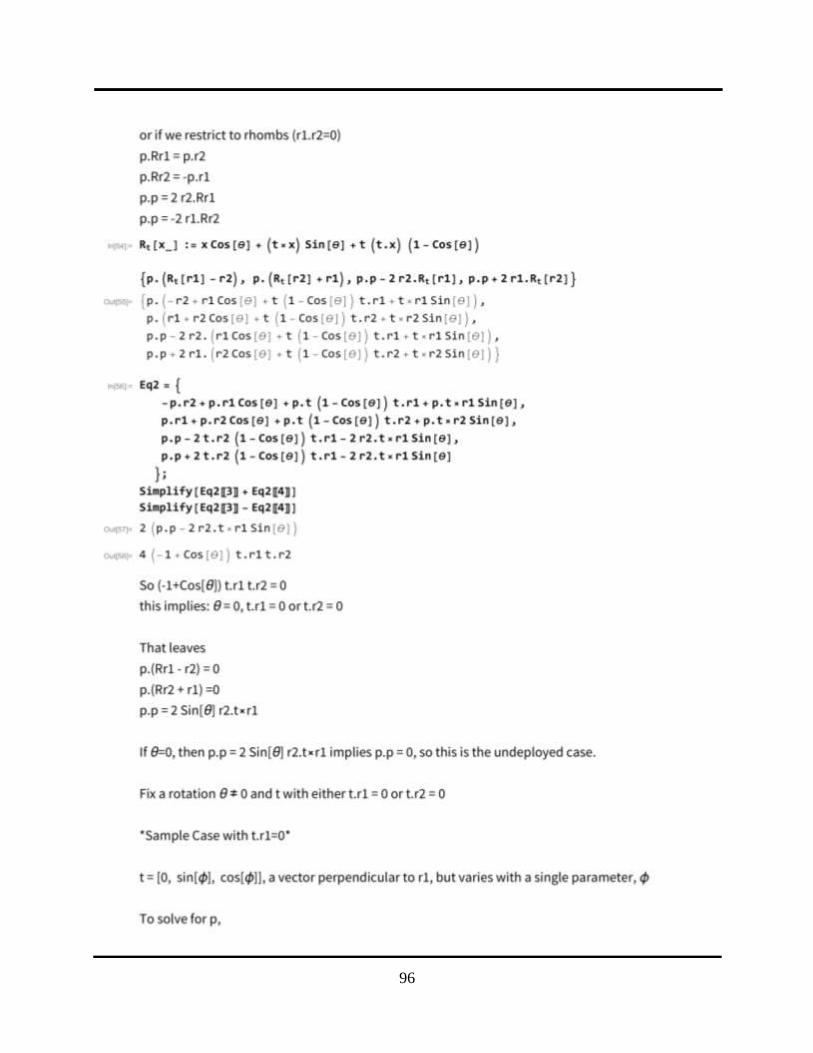
96

97

98
THIS PAGE INTENTIONALLY LEFT BLANK

99
Appendix B: Sample Calculation of
Deployment in Mathematica
This appendix contains a Mathematica script for a sample calculation of the algorithm derived in
Chapter 5.

100
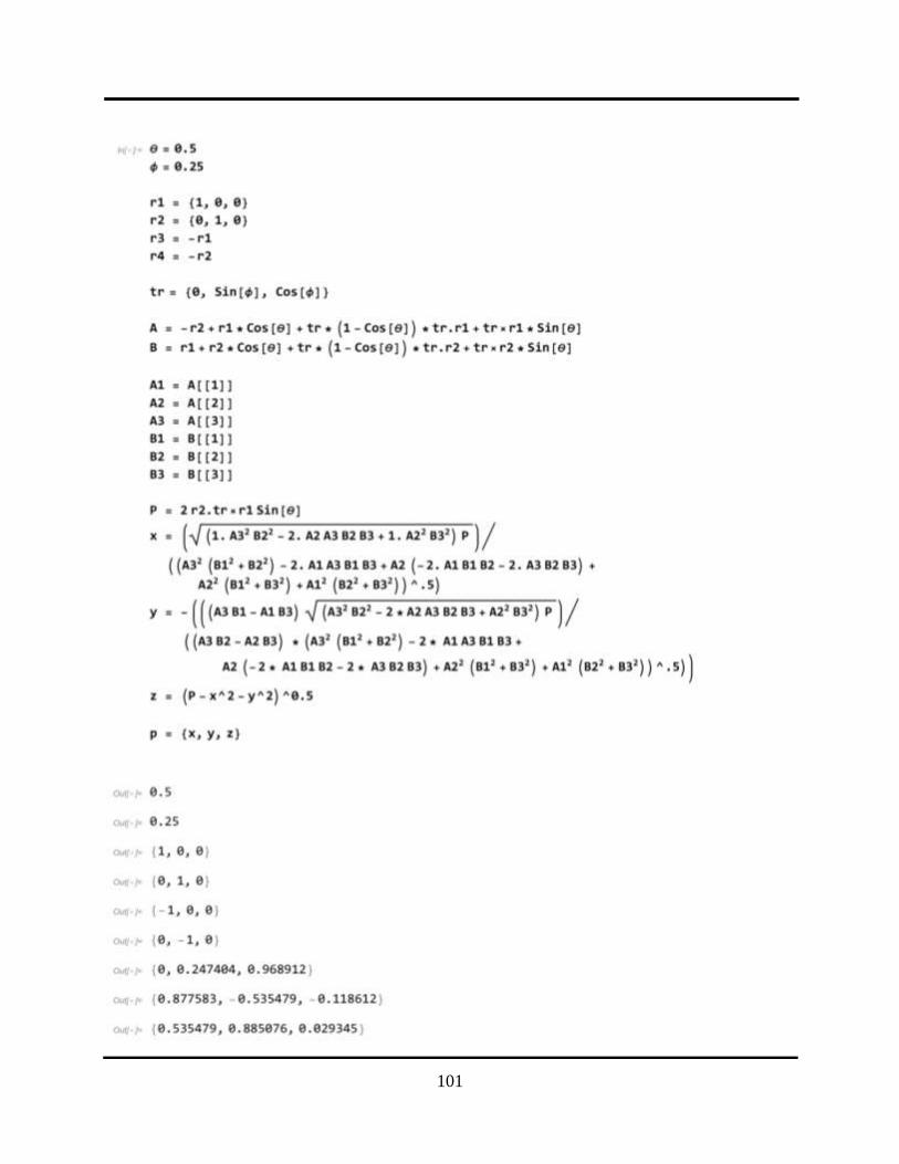
101

102

103

104

105
Appendix C: Computational Primary Surface
Python Script
This appendix contains the Python script for the creation of a computationally produced primary
surface for the kirigami space frame. This code is broken into five parts: Objective, File_Read,
Kirigami, Distance, and Plot.
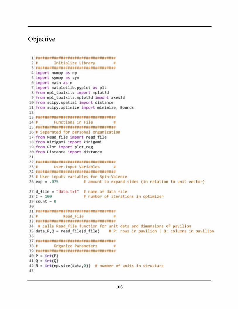
106
Objective

107
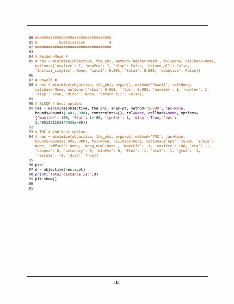
108
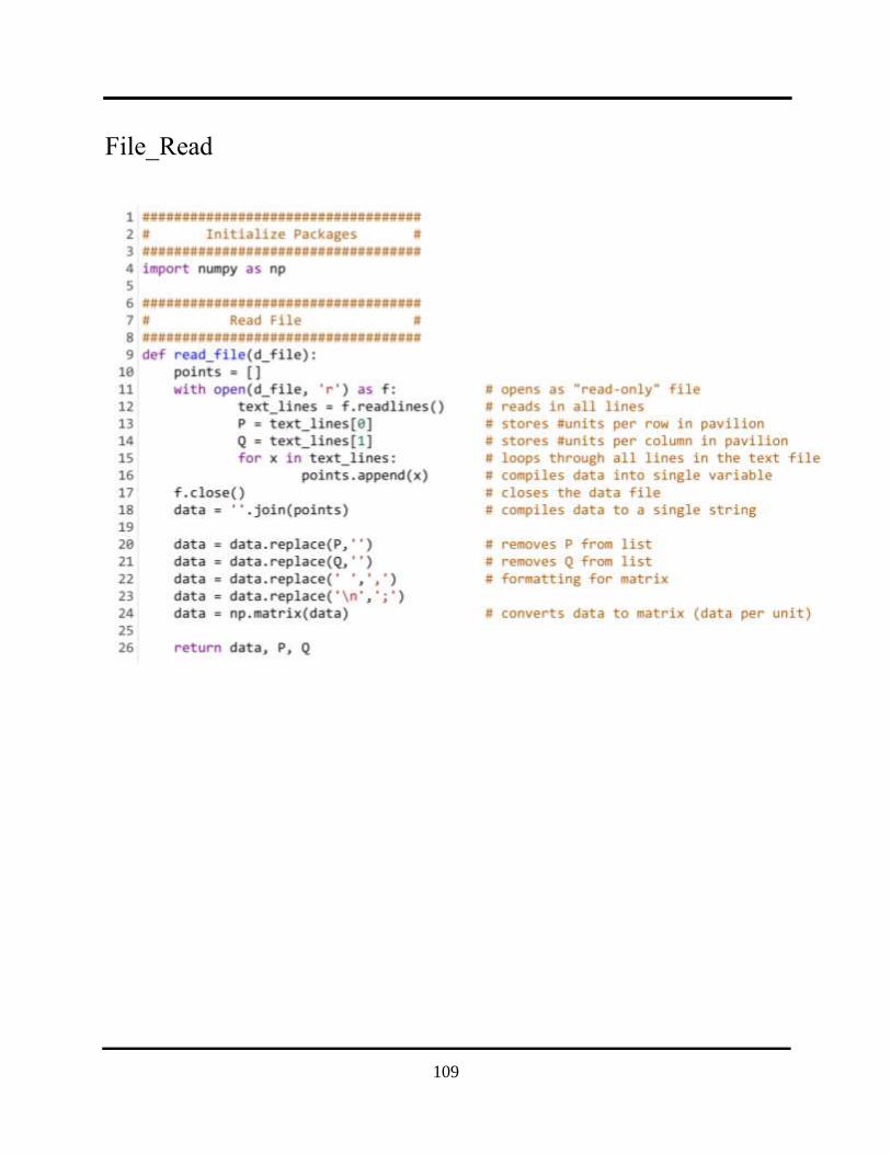
109
File_Read

110
Kirigami

111

112
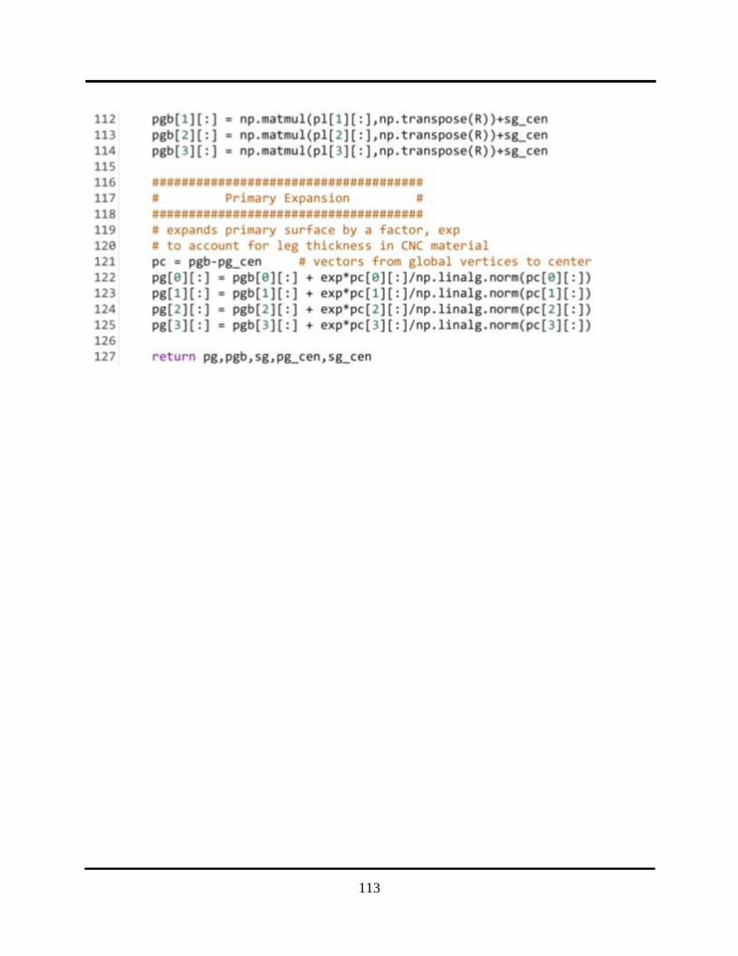
113

114
Distance

115

116
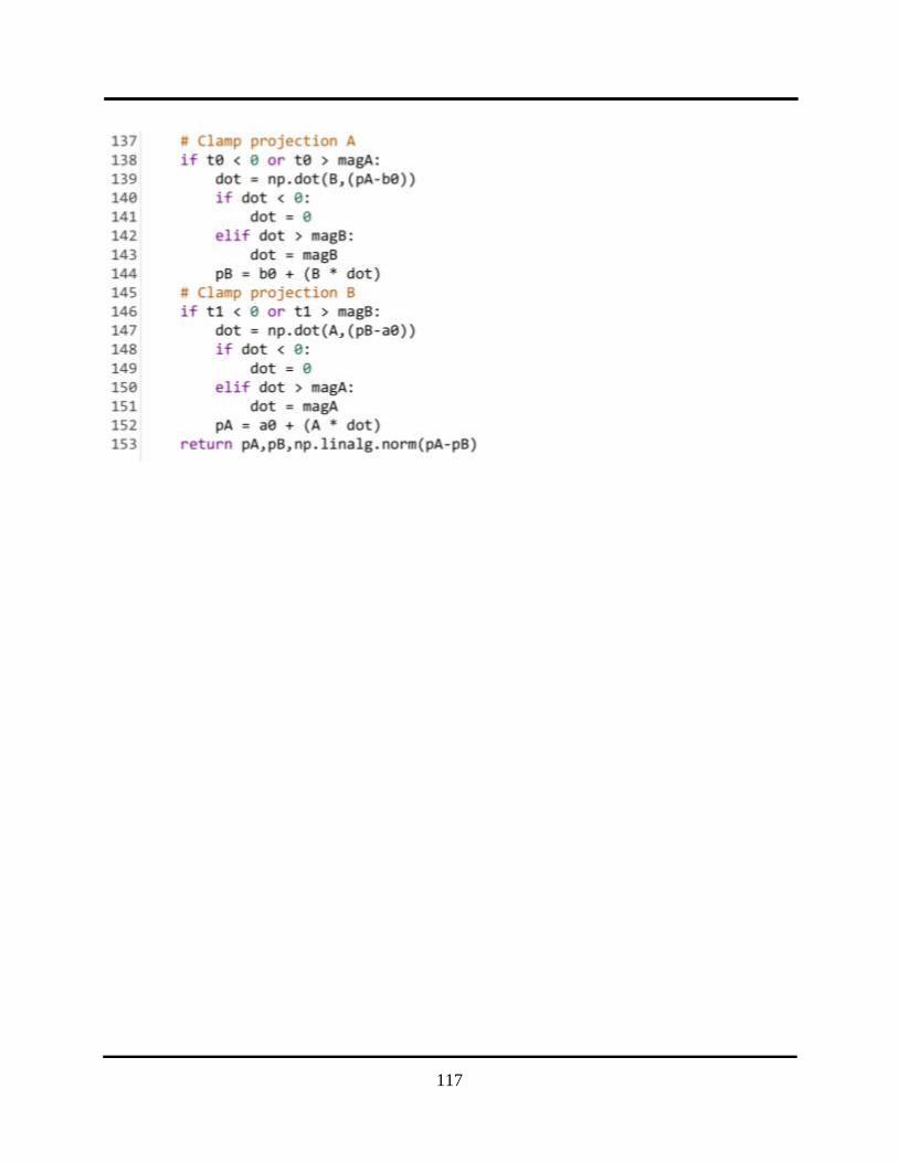
117

118
Plot

119

120
THIS PAGE INTENTIONALLY LEFT BLANK

121
Appendix D: Additional Images from
Chapter 6 Results
This appendix contains the additional images for the optimization results from Section 6.5.10.

122
3x14 Assembly
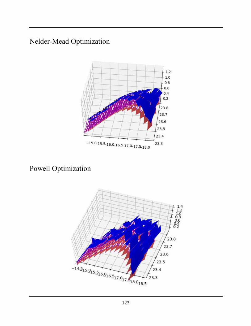
123
Nelder-Mead Optimization
Powell Optimization

124
TNC Optimization

125
SLSQP Optimization

126
Non-Optimized Pavilion

127
TNC Optimized Pavilion

128
SLSQP Optimized Pavilion